Embed Size (px)
Citation preview

HCI/ComS 575X:
Computational Perception
Instructor: Alexander Stoytchevhttp://www.cs.iastate.edu/~alex/classes/2006_Spring_575X/

The Kalman Filter(part 2)
HCI/ComS 575X: Computational PerceptionIowa State University, SPRING 2006Copyright © 2006, Alexander Stoytchev
February 15, 2006

Brown and Hwang (1992)
“Introduction to Random Signals and Applied Kalman Filtering”
Ch 5: The Discrete Kalman Filter

Maybeck, Peter S. (1979)
Chapter 1 in ``Stochastic models, estimation, and control'',
Mathematics in Science and Engineering Series, Academic
Press.

A Simple Recursive Example
• Problem Statement:
Given the measurement sequence:
z1, z2, …, zn find the mean
[Brown and Hwang (1992)]

First Approach
1. Make the first measurement z1
Store z1 and estimate the mean as
µ1=z1
2. Make the second measurement z2
Store z1 along with z2 and estimate the mean as
µ2= (z1+z2)/2
[Brown and Hwang (1992)]

First Approach (cont’d)
3. Make the third measurement z3
Store z3 along with z1 and z2 and
estimate the mean as
µ3= (z1+z2+z3)/3
[Brown and Hwang (1992)]

First Approach (cont’d)
n. Make the n-th measurement zn
Store zn along with z1 , z2 ,…, zn-1 and
estimate the mean as
µn= (z1 + z2 + … + zn)/n
[Brown and Hwang (1992)]

Second Approach
1. Make the first measurement z1
Compute the mean estimate as
µ1=z1
Store µ1 and discard z1
[Brown and Hwang (1992)]

Second Approach (cont’d)
2. Make the second measurement z2
Compute the estimate of the mean as aweighted sum of the previous estimate
µ1 and the current measurement z2:
µ2= 1/2 µ1 +1/2 z2
Store µ2 and discard z2 and µ1
[Brown and Hwang (1992)]

Second Approach (cont’d)
3. Make the third measurement z3
Compute the estimate of the mean as aweighted sum of the previous estimate
µ2 and the current measurement z3:
µ3= 2/3 µ2 +1/3 z3
Store µ3 and discard z3 and µ2
[Brown and Hwang (1992)]

Second Approach (cont’d)
n. Make the n-th measurement zn
Compute the estimate of the mean as aweighted sum of the previous estimate µn-1 and the current measurement zn:
µn= (n-1)/n µn-1 +1/n zn
Store µn and discard zn and µn-1
[Brown and Hwang (1992)]

Analysis
• The second procedure gives the same result as the first procedure.
• It uses the result for the previous step to help obtain an estimate at the current step.
• The difference is that it does not need to keep the sequence in memory.
[Brown and Hwang (1992)]
A simple example using diagrams

Conditional density of position based on measured value of z1
[Maybeck (1979)]

Conditional density of position based on measured value of z1
[Maybeck (1979)]
position
measured position
uncertainty

Conditional density of position based on measurement of z2 alone
[Maybeck (1979)]

Conditional density of position based on measurement of z2 alone
[Maybeck (1979)]measured position 2
uncertainty 2

Conditional density of position based on data z1 and z2
[Maybeck (1979)]position estimate
uncertainty estimate

Propagation of the conditional density
[Maybeck (1979)]

Propagation of the conditional density
[Maybeck (1979)]
movement vector
expected position just prior to taking measurement 3

Propagation of the conditional density
[Maybeck (1979)]
movement vector
expected position just prior to taking measurement 3
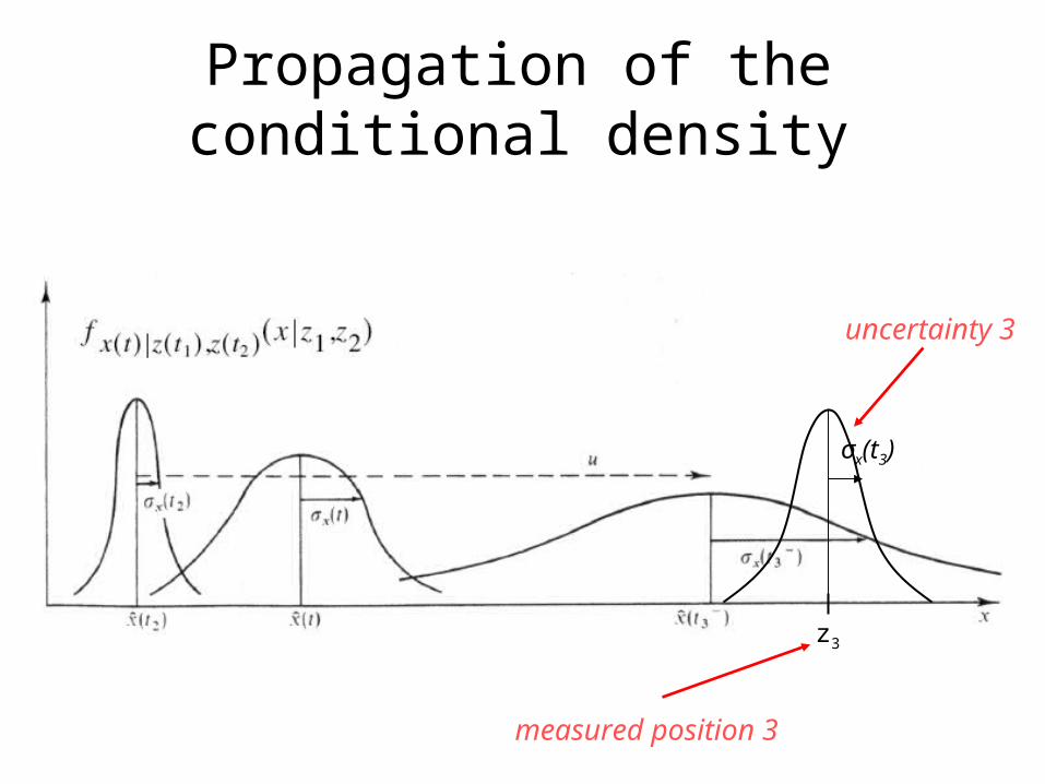
Propagation of the conditional density
z3
σx(t3)
measured position 3
uncertainty 3

Updating the conditional density after the third measurement
z3
σx(t3)
position uncertainty
position estimate
x(t3)


Questions?

Now let’s do the same thing…but this time we’ll use math
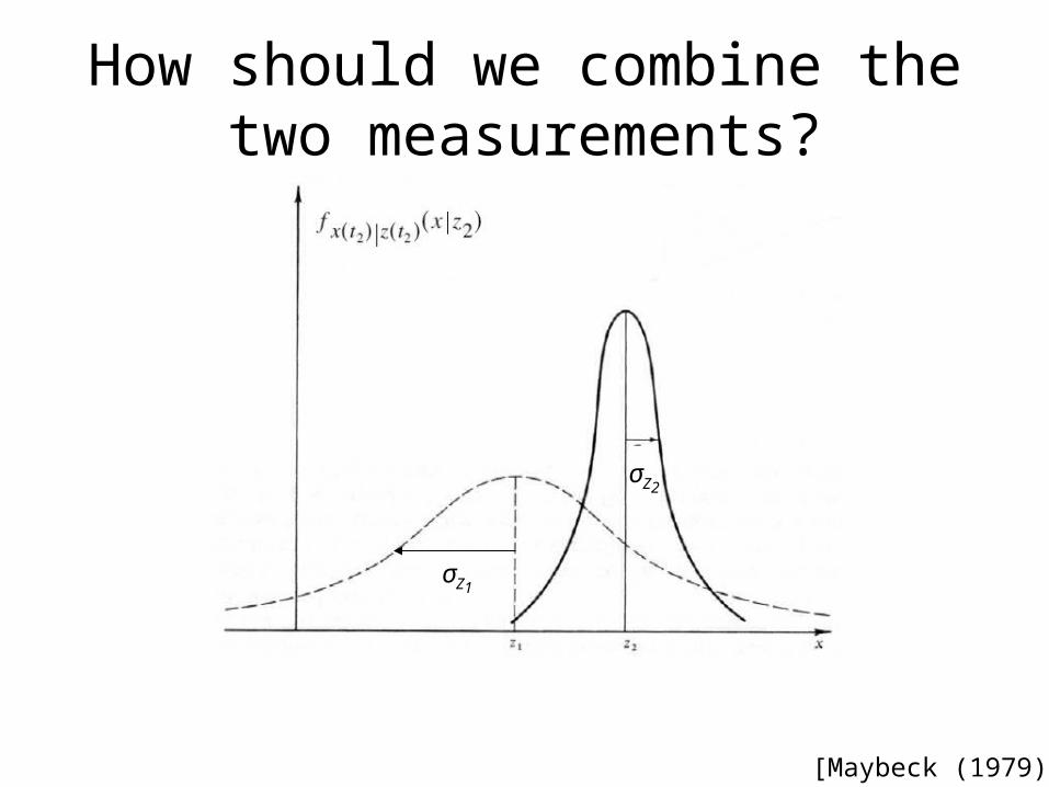
How should we combine the two measurements?
[Maybeck (1979)]
σZ1
σZ2

Calculating the new mean
Scaling Factor 1 Scaling Factor 2
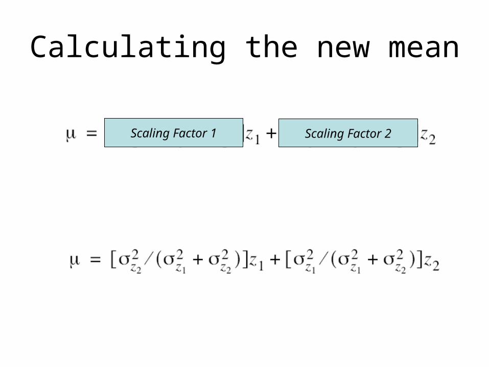
Calculating the new mean
Scaling Factor 1 Scaling Factor 2

Calculating the new mean
Scaling Factor 1 Scaling Factor 2
Why is this not z1?

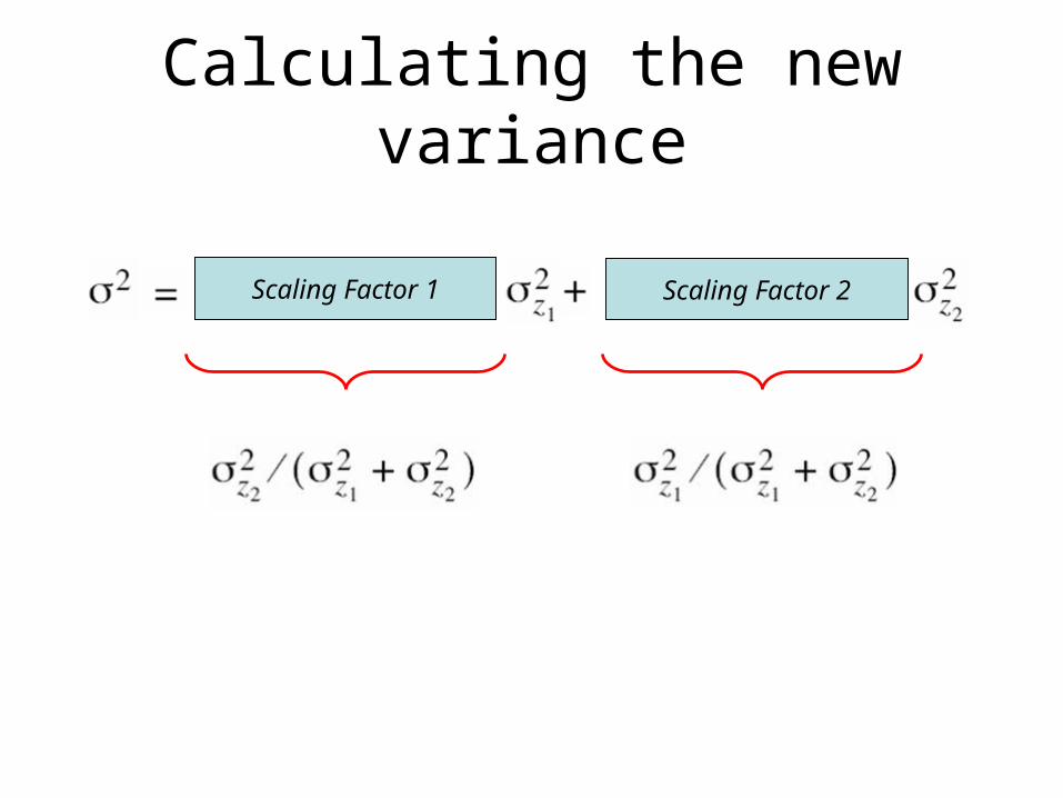
Calculating the new variance
[Maybeck (1979)]
σZ1
σZ2

Calculating the new variance
Scaling Factor 1 Scaling Factor 2
Calculating the new variance
Scaling Factor 1 Scaling Factor 2

Calculating the new variance
Scaling Factor 1 Scaling Factor 2

Calculating the new variance

Calculating the new variance

Calculating the new variance

Why is this result different from the one given in the paper?

Remember the Gaussian Properties?

Remember the Gaussian Properties?
• If and
• Then
This is a2 not a

The scaling factors must be squared!
Scaling Factor 1 Scaling Factor 2

Therefore the new variance is
Try to derive this on your own.

Another Way to Express The New Position
[Maybeck (1979)]

Another Way to Express The New Position
[Maybeck (1979)]

Another Way to Express The New Position
[Maybeck (1979)]

The equation for the variance can also be rewritten as
[Maybeck (1979)]

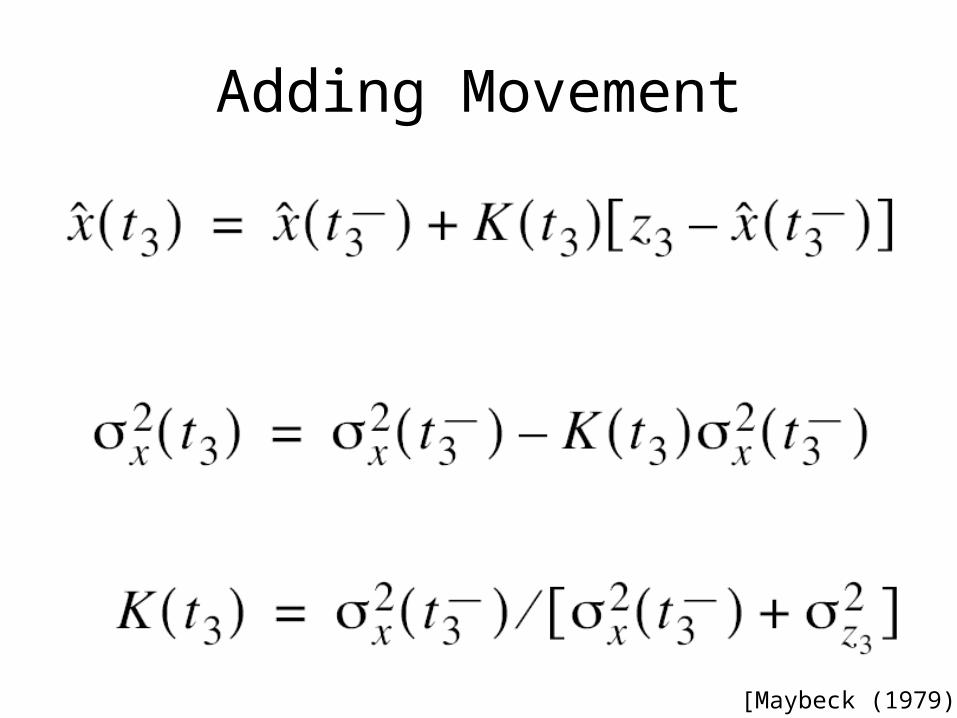
Adding Movement
[Maybeck (1979)]

Adding Movement
[Maybeck (1979)]
Adding Movement
[Maybeck (1979)]

Properties of K
• If the measurement noise is large K is small
0
[Maybeck (1979)]

Another Example

A Simple Example
• Consider a ship sailing east with a perfect compass trying to estimate its position.
• You estimate the position x from the stars as z1=100 with a precision of σx=4 miles
x100
[www.cse.lehigh.edu/~spletzer/cse398_Spring05/lec011_Localization2.ppt]

A Simple Example (cont’d)
• Along comes a more experienced navigator, and she takes her own sighting z2
• She estimates the position x= z2 =125 with a precision of σx=3 miles
• How do you merge her estimate with your own?
x100 125
[www.cse.lehigh.edu/~spletzer/cse398_Spring05/lec011_Localization2.ppt]

A Simple Example (cont’d)
xx2=116
2221
2
1221
2
2
1
2
2 zzzz
z
zz
z
116125916
16100
916
9
222
21
111
zz
4.2144
25
16
1
9
112
[www.cse.lehigh.edu/~spletzer/cse398_Spring05/lec011_Localization2.ppt]

• With the distributions being Gaussian, the best estimate for the state is the mean of the distribution, so…
or alternately
where Kt is referred to as the Kalman gain, and must be computed at each time step
)(
)(
1221
1222
2
1
21
1
zzKz
zzzzz
z
A Simple Example (cont’d)
2221
2
122
2
2
2
1
21
2 zzxzz
z
zz
z
Correction Term
[www.cse.lehigh.edu/~spletzer/cse398_Spring05/lec011_Localization2.ppt]

• OK, now you fall asleep on your watch. You wake up after 2 hours, and you now have to re-estimate your position
• Let the velocity of the boat be nominally 20 miles/hour, but with a variance of σ2
w=4 miles2/hour
• What is the best estimate of your current position?
A Simple Example (cont’d)
xx2=116 x-3 =?
[www.cse.lehigh.edu/~spletzer/cse398_Spring05/lec011_Localization2.ppt]

• The next effect is that the gaussian is translated by a distance and the variance of the distribution is increased to account for the uncertainty in dynamics
A Simple Example (cont’d)
t
tvxx
w
222
23
23
76.13876.5
1564011623
3
x
xx2=116 x-3 =156
[www.cse.lehigh.edu/~spletzer/cse398_Spring05/lec011_Localization2.ppt]

• OK, this is not a very accurate estimate. So, since you’ve had your nap you decide to take another measurement and you get z3=165 miles
• Using the same update procedure as the first update, we obtain
and so on…
A Simple Example (cont’d)
)( 33333 xzKxx
233
23
23 K
40.776.131676.13
76.1376.13
[www.cse.lehigh.edu/~spletzer/cse398_Spring05/lec011_Localization2.ppt]

• In this example, prediction came from using knowledge of the vehicle dynamics to estimate its change in position
• An analogy with a robot would be integrating information from the robot kinematics (i.e. you give it a desired [x, y, α] velocities for a time Δt) to estimate changed in position
• The correction is accomplished through making exteroceptive observations and then fusing this with your current estimate
• This is akin to updating position estimates using landmark information, etc.
• In practice, the prediction rate is typically much higher than the correction
The Predictor-Corrector Approach[www.cse.lehigh.edu/~spletzer/cse398_Spring05/lec011_Localization2.ppt]


Kalman Filter Diagram
[Brown and Hwang (1992)]

The process to be estimated


THE END