HDF5 FastQueryAccelerating Complex Queries on HDF Datasets using Fast Bitmap

IndicesJohn Shalf, Wes Bethel

LBNL Visualization Group

Kensheng Wu, Kurt Stockinger

LBNL SDM CenterLuke Gosink, Ken Joy

UC Davis IDAV

QuickTime™ and aTIFF (Uncompressed) decompressorare needed to see this picture.

Motivation and Problem Statement

• Too much data.• Visualization “meat grinders”

not especially responsive to needs of scientific research community.

• What scientific users want:– Scientific Insight– Quantitative results– Feature detection, tracking,

characterization– (lots of bullets here omitted)

• See:http://vis.lbl.gov/Publications/2002/

VisGreenFindings-LBNL-51699.pdfhttp://www-user.slac.stanford.edu/rmount/dm-

workshop-04/Final-report.pdf

Motivation and Problem Statement

• Too much data.• Visualization “meat grinders”

not especially responsive to needs of scientific research community.

• What scientific users want:– Scientific Insight– Quantitative results– Feature detection, tracking,

characterization– (lots of bullets here omitted)

• See:http://vis.lbl.gov/Publications/2002/

VisGreenFindings-LBNL-51699.pdfhttp://www-user.slac.stanford.edu/rmount/dm-

workshop-04/Final-report.pdf

What is FastBit?(what is it’s role in data analysis?)

Using Indexing Technology to Accelerate Data Analysis

• Use cases for indexed datasets– Support Compound Range Queries: eg. Get me all cells where

Temperature > 300k AND Pressure is < 200 millibars– Subsetting: Only load data that corresponds to the query.

• Get rid of visual “clutter”• Reduce load on data analysis pipeline

– Quickly find and label connected regions– Do it really fast!

• Applications– Astrophysics:

• Remove clutter from messy supernova explosions

– Combustion: • Locate and track ignition kernels

– Particle Accelerator Modeling: • identify and select errant electrons

– Network Security Data: • Pose queries against enormous packet logs• Identify candidate security events

Architecture Overview: Generic Visualization Pipeline

DataVis /

AnalysisDisplay

Architecture Overview: Query-Driven Vis. Pipeline

Vis /Analysis

Display

Index

DataQuery

FastBit

Query-Driven Subsetting of Combustion Data Set

b) Q: temp < 3

c) Q: CH4 > 0.3 AND temp < 3

d) Q: CH4 > 0.3 AND temp < 4

a) Query: CH4 > 0.3

DEX Visualization Pipeline

DataQuery

Visualization Toolkit(VTK)

3D visualization of aSupernova explosion

Architecture Overview: Query-Driven Analysis Pipeline

Vis /Analysis

Display

Index

Data Query

FastBit

HDF4NetCDFBinary

Architecture Overview: Query-Driven Analysis Pipeline

Vis /Analysis

DisplayHDF5Data+Index

Query

FastBit

How do Fast Bitmap Indices Work?

Why Bitmap Indices?

• Goal: efficient search of multi-dimensional read-only (append-only) data:– E.g. temp < 104.5 AND velocity > 107 AND density < 45.6

• Commonly-used indices are designed to be updated quickly– E.g. family of B-TreesB-Trees– Sacrifice search efficiency to permit dynamic update

• Most multi-dimensional indices suffer curse of dimensionality– E.g. R-tree, Quad-trees, KD-treesR-tree, Quad-trees, KD-trees, …– Don’t scale to large number of dimensions ( < 10)– Are efficient only if all dimensions are queried

• Bitmap indices – Sacrifice update efficiency to gain more search efficiency– Are efficient for multi-dimensional queries– Query response time scales linearly in the actual number of

dimensions in the query

What is a Bitmap Index?

• Compact: one bit per distinct value per object.

• Easy and fast to build: O(n) vs. O(n log n) for trees.

• Efficient to query: use bitwise logical operations.(0.0 < H2O < 0.1) AND (1000 <

temp < 2000)

• Efficient for multidimensional queries.– No “curse of dimensionality”

• What about floating-point data?– Binning strategies.

Datavalues

015312041

100000100

010010001

000001000

000100000

000000010

001000000

b0 b1 b2 b3 b4 b5

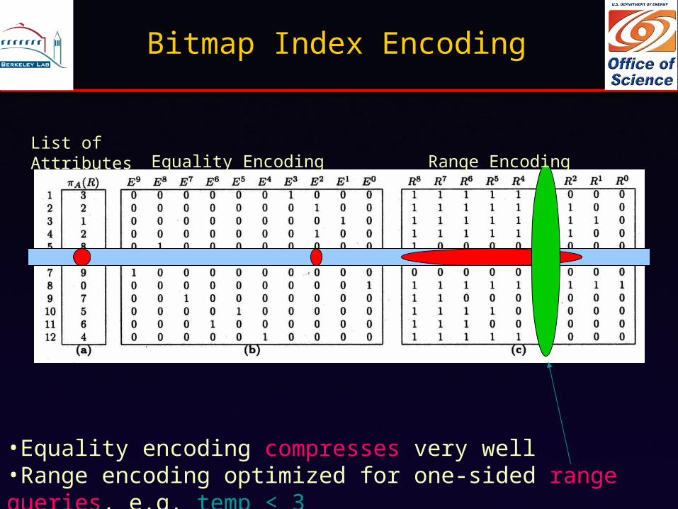
Bitmap Index Encoding

•Equality encoding compresses very well•Range encoding optimized for one-sided range queries, e.g. temp < 3

List of Attributes Equality Encoding Range Encoding

Performance

Bitmap Index Query Complexity and Space Requirements

• How Fast are Queries Answered?– Let N denote the number of objects and H denote the number of

hits of a condition.– Using uncompressed bitmap indices, search time is O(N)– With a good compression scheme, the search time is O(H) – the

theoretical optimum

• How Big are the Indices?– In the worst case (completely random data), the bitmap index

requires about 2x in data size for one variable (typically 0.3x).– In contrast, 4x space requirement not uncommon for tree-based

methods for one variable.– Curse of dimensionality: for N points in D dimensions:

• Bitmap index size: O(D*N)• Tree-based method: O(N**D)!!!

Compressed Bitmap Index Query Performance

• FastBit Word-Aligned Hybrid (WAH) compression performance better than commercial systems.

• Different bitmap compression technologies have different performance characteristics.

Queries Using Bitmap Indices are Fast

Log-log plot of query processing time for different size queries

The compressed bitmap index is at least 10X faster than B-tree and 3X faster than the projection index

Size of Bitmap Index vs. Base Data (Combustion)

Average size per attribute index

0

5,000,000

10,000,000

15,000,000

20,000,000

25,000,000

base data

uz

pressure

uytemp

N2 ux O2 CH4 CO2 H2O

Attribute

Size [bytes]

Total size of all indices vs. base data size

0

20,000,000

40,000,000

60,000,000

80,000,000

100,000,000

120,000,000

base data bitmap index

Size [bytes]

• Compressed bitmap index with 100 range-encoded bins is about same size as base data.

• Note: B-tree index is about 3 times the size of the base data.• Building the index takes ~5 seconds for 100Megs on P4 2.4GHz

workstation

Size of Bitmap Index vs. Base Data (Astrophysics)

• Size of compressed bitmap index is only 57% of base data.• Building an index for all attributes takes ~17 seconds for 340 Megs.

Average size per attribute index

0

10,000,000

20,000,000

30,000,000

40,000,000

50,000,000

60,000,000

70,000,000

80,000,000

base data x_velocity density y_velocity z_velocity pressure entropy

Attribute

Size [bytes]

Total size of all indices vs. base data size

0

50,000,000

100,000,000

150,000,000

200,000,000

250,000,000

300,000,000

350,000,000

base data bitmap index

Size [bytes]

Region Growing andConnected Component Labeling

• The result of the bitmap index query is a set of blocks.

• Given a set of blocks, find connected regions and label them.

0

0.2

0.4

0.6

0.8

1

1.2

1.4

1.6

1.8

10000 110000 210000 310000 410000

Number of line segments

region growing time (sec)

• Region growing scales linearly with the number of cells selected.

HDF5 - FastQuery File Organization

File Organization

• Current– Data in HDF4, NetCDF converted to raw binary– One file per species + one file per index– ASCII file for metadata– One directory per timestep– Non-portable binary (must byte-swap data)

• HDF5 FastQuery– Indices + data all in same file– Machine independent binary representation– Multiple time-steps per file– Pose queries against data stored in “indexed” HDF5 file

Some Simplifying Assumptions

• Block structured data– 0-3 Dimensional topology (arbitrary geometry)– Limited Datatypes: float, double, int32, int64, byte– Vectors and Tensors identified via metadata

• Two Level hierarchical organization– TimeStep– VariableName– Queries can be posed implicitly across time dimension

• Future– Arbitrary nesting

• AMR “Level”• CalibrationSet

– More Data Schemas• Unstructured• AMR• NetLogs

/H5_UC

Descriptorfor

Variable 1

Descriptorfor

Variable X

Descriptorfor

Variable 0… Time Step 1 Time Step YTime Step 0 …

Variable DescriptorsVariable Data

D0

D1

DX

D0

D1

DX

D0

D1

DX… … …

HDF5 Data Organization to Support FastQuery

HDF5 ROOT Group

Symbol KeyHDF5 group:Contains user retrievable informationabout sub-groups and datasets

HDF5 dataset:Contains the actual data array of a given variable X at a time step Y

X variable descriptorsfor X datasets

TOC

File Organization

Bitm

ap Indices

D2(Base Data)

Time Step 0

D0

D1

File Organization

Bitm

ap Indices

D2(Base Data)

Name=“Pressure”Dims={64,64,64}Type=Double

Name=“Pressure.idx”Dims=0.3*datasizeType=Int32

Time Step 0

D0

D1

File Organization

Bitm

ap Indices

BinsBase Data

Offsets

File Organization

Bitm

ap Indices

BinsBase Data

Offsets

AttributeName=“offsets”Dims=nbins-1Type=uInt64

AttributeName=“bins”Dims=2*nbins or nbinsType=Double(same type as data)

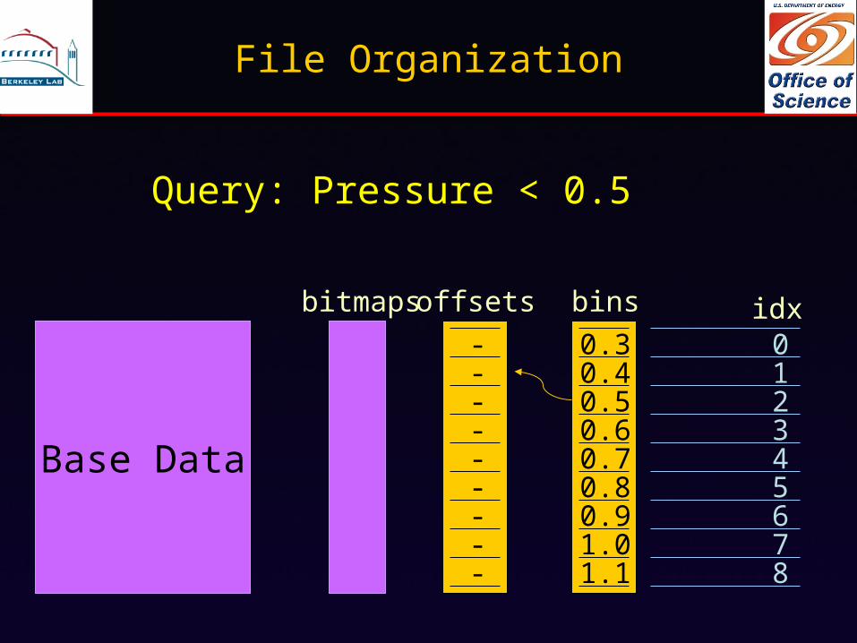
File Organization

Base Data

012345678

idxbinsoffsetsbitmaps

0.30.4

0.60.5

0.70.80.91.01.1

Query: Pressure < 0.5

---------

File Organization

Base Data

012345678

idxbinsoffsetsbitmaps

0.30.4

0.60.5

0.70.80.91.01.1

Query: Pressure < 0.5

---------

File Organization

Base Data

012345678

idxbinsoffsetsbitmaps

0.30.4

0.60.5

0.70.80.91.01.1

Query: Pressure < 0.5

-158239

------

File Organization

Base Data

012345678

idxbinsoffsetsbitmaps

0.30.4

0.60.5

0.70.80.91.01.1

Query: Pressure < 0.5

---------

Final Notes

• Need for Higher level data organization– Demonstrated simple convention for index storage– Require higher level data organization to support more

complex queries demanded by our scientific applications– Adoption of higher-level schema is a sociological problem

rather than a technical problem

• Top Down (the Grand Unified Data Model)– DMF: Describe everything in the known universe

• Bottom up (community building)– Research Group: Store data fro Cactus– Scientific Community: eg. HDF-EOS, NetCDF, FITS– ?

Final Notes

• Need for Higher level data organization– Demonstrated simple convention for index storage– Require higher level data organization to support more

complex queries demanded by our scientific applications– Adoption of higher-level schema is a sociological problem

rather than a technical problem

• Top Down (the Grand Unified Data Model)– DMF: Describe everything in the known universe

• Bottom up (community building)– Research Group: Store data fro Cactus– Scientific Community: eg. HDF-EOS, NetCDF, FITS– World Domination

Questions?

Performance of Event Catalog

• The Event Catalog uses compressed bitmap indices– The most commonly used index is B-tree– The most efficient one is often the projection index

• The following table reports the size and the average query processing time– 1-attribute, 2-attribute, and 5-attribute refer to the number of attributes in a

query

• Compressed bitmap indices are about half the size of B-trees, and are 10 times faster

• Compressed bitmap indices are larger than projection indices, but are 3 times faster

2.2 Million Events

12 common attributes

B-tree Projection

index

Bitmap

indexSize (MB) 408 113 186Query processing

(seconds)

1-attribute 0.95 0.51 0.022-attribute 2.15 0.56 0.045-attribute 2.23 0.67 0.17