UNIVERSITY OF CALIFORNIA Economics 134 DEPARTMENT OF ECONOMICS Spring 2018

Professor David Romer

LECTURE 4

REVIEW OF IS–LM/MP FRAMEWORK JANUARY 29, 2018

I. THE IS–LM/MP MODEL A. Overview 1. Introduction 2. Where we are headed 3. A key assumption 4. A general comment about models B. Review of the IS Curve 1. Planned expenditure and output 2. Modeling planned expenditure 3. The Keynesian cross 4. Deriving the IS curve C. One Approach to the Other Curve: The MP Curve 1. An interest rate rule 2. The MP curve and the IS-MP diagram 3. But how is the central bank able to control the real interest rate? D. Another Approach to the Other Curve: The LM Curve 1. Introduction 2. The concept of money we will focus on 3. The supply and demand for money 4. The interest rate for a given level of output: the money market 5. Deriving the LM curve E. MP or LM? II. EXAMPLES A. A Fall in Investment Demand 1. The shock 2. The effects when the central bank follows an interest rate rule 3. The effects when the central bank targets the money supply B. Financial Innovation 1. The shock 2. The effects when the central bank targets the money supply 3. The effects when the central bank follows an interest rate rule

LECTURE 4 Review of IS–LM/MP Framework

January 29, 2018

Economics 134 David Romer Spring 2018

Housekeeping

• The reading for next time (“A Non-Technical Introduction to Regressions”) is in the main course reader, after the “Short-Run Fluctuations” material.

• Reminder: The final exam is Monday, May 7, 3–6 P.M.

I. THE IS–LM/MP MODEL

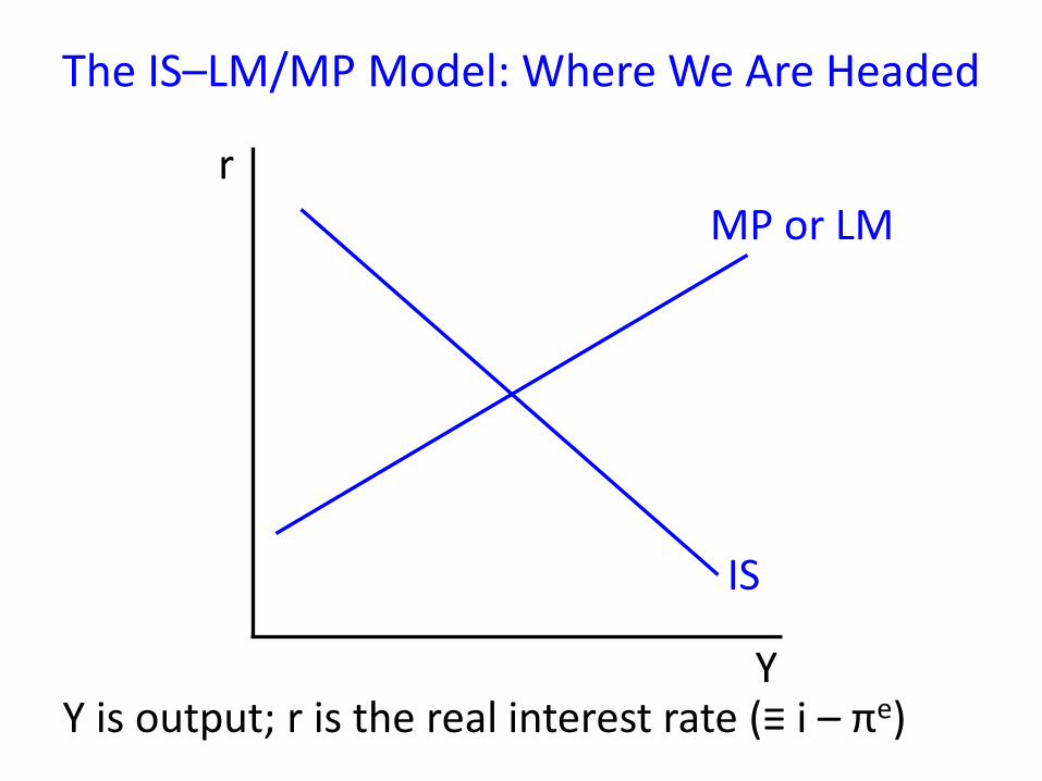
Y

r MP or LM

IS

The IS–LM/MP Model: Where We Are Headed

Y is output; r is the real interest rate (≡ i – πe)

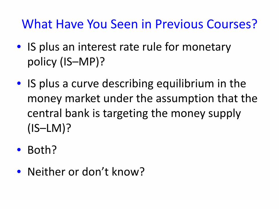
What Have You Seen in Previous Courses?

• IS plus an interest rate rule for monetary policy (IS–MP)?

• IS plus a curve describing equilibrium in the money market under the assumption that the central bank is targeting the money supply (IS–LM)?

• Both?

• Neither or don’t know?

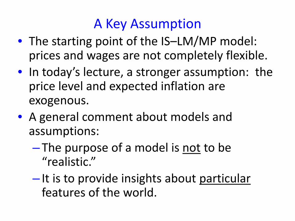
A Key Assumption • The starting point of the IS–LM/MP model:

prices and wages are not completely flexible. • In today’s lecture, a stronger assumption: the

price level and expected inflation are exogenous.

• A general comment about models and assumptions: – The purpose of a model is not to be

“realistic.” – It is to provide insights about particular

features of the world.

The Equations of the IS Curve #1: Planned Expenditure and Output

E = Y E is planned expenditure, Y is output.

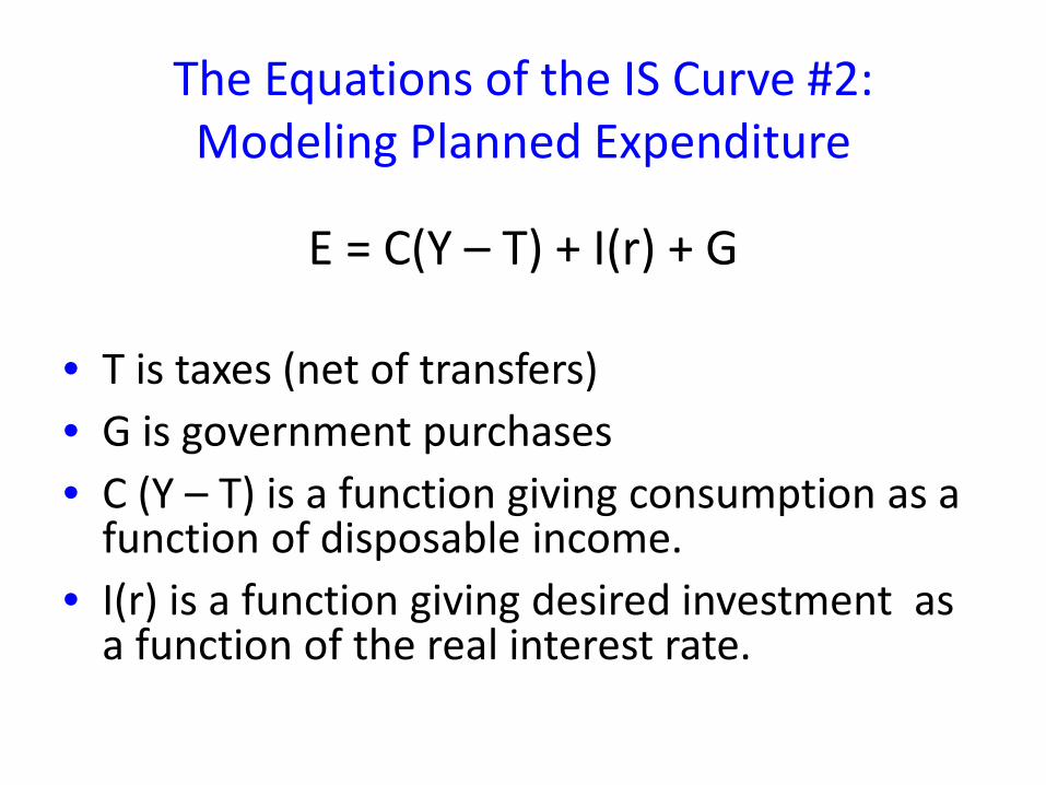
The Equations of the IS Curve #2: Modeling Planned Expenditure

E = C(Y – T) + I(r) + G

• T is taxes (net of transfers) • G is government purchases • C (Y – T) is a function giving consumption as a

function of disposable income. • I(r) is a function giving desired investment as

a function of the real interest rate.

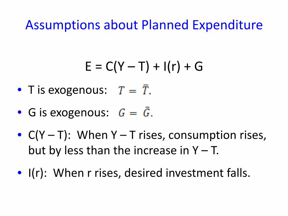
Assumptions about Planned Expenditure

E = C(Y – T) + I(r) + G

• T is exogenous:

• G is exogenous:

• C(Y – T): When Y – T rises, consumption rises, but by less than the increase in Y – T.

• I(r): When r rises, desired investment falls.

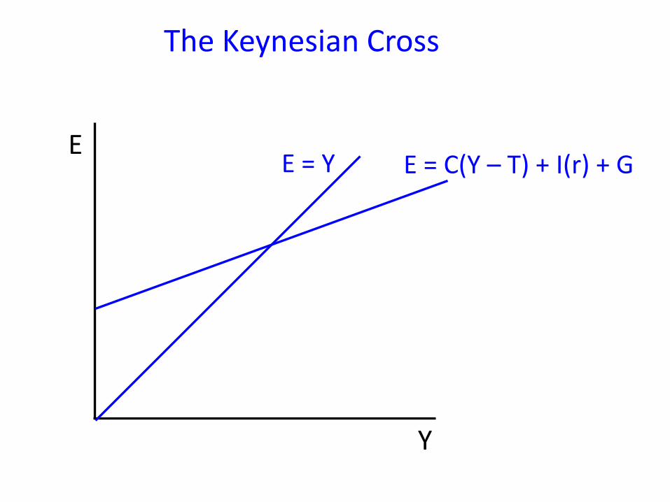
The Keynesian Cross

Y

E E = Y E = C(Y – T) + I(r) + G

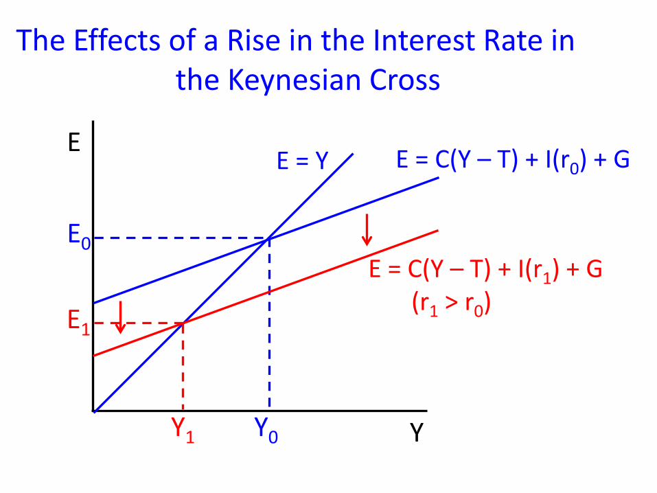
The Effects of a Rise in the Interest Rate in the Keynesian Cross

Y

E E = Y E = C(Y – T) + I(r0) + G

E0

Y0

E = C(Y – T) + I(r1) + G (r1 > r0) E1

Y1

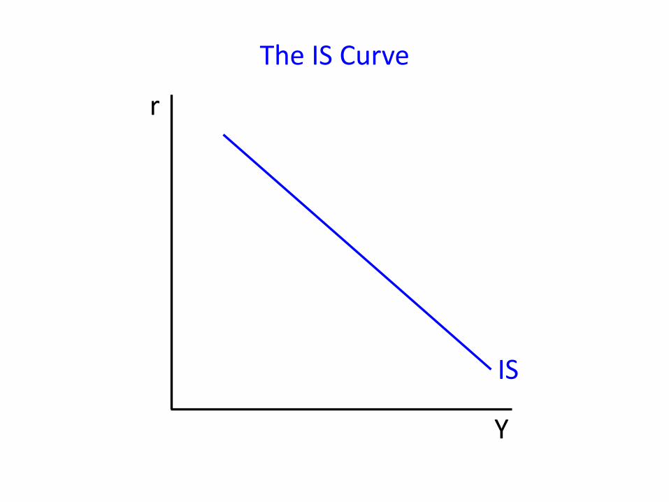
The IS Curve

Y

r

IS

One Approach to the Other Curve: An Interest Rate Rule and the MP Curve

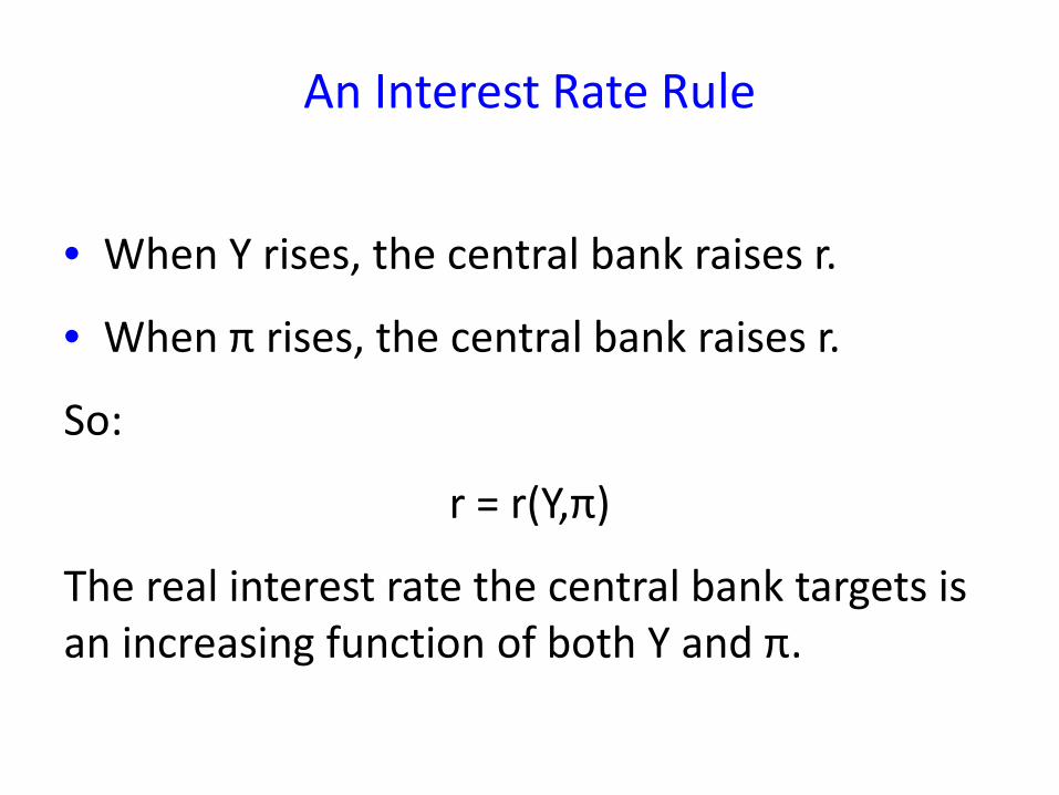
An Interest Rate Rule

• When Y rises, the central bank raises r.

• When π rises, the central bank raises r.

So:

r = r(Y,π)

The real interest rate the central bank targets is an increasing function of both Y and π.

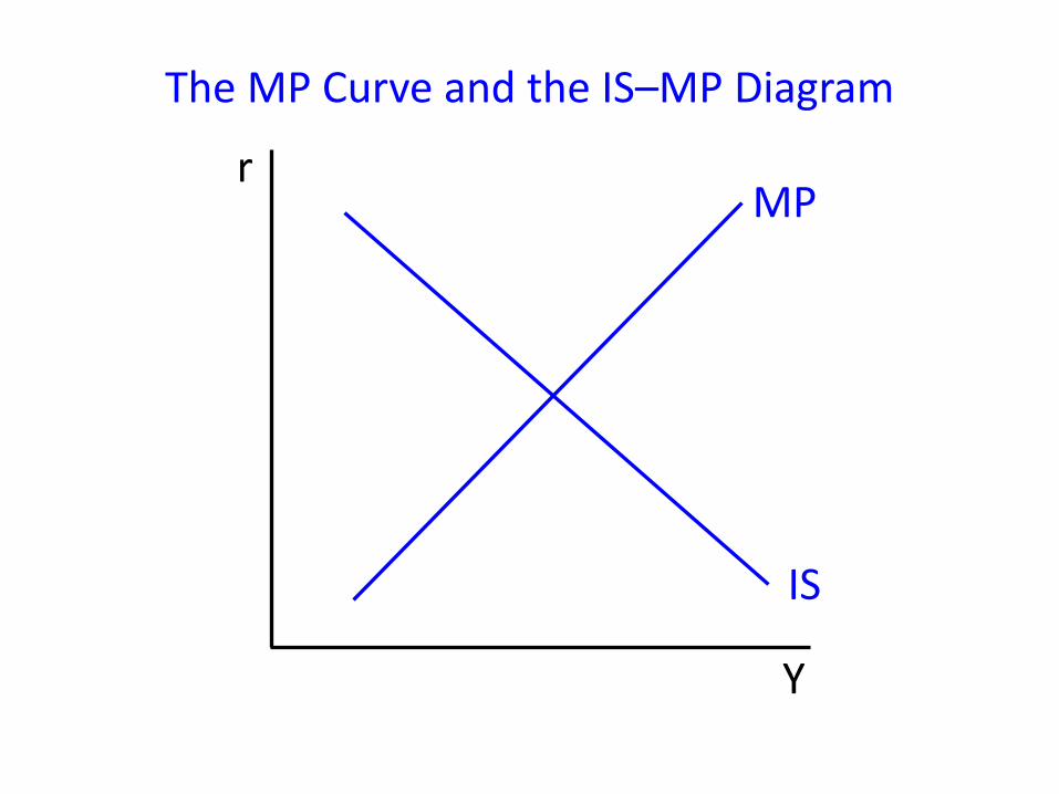
The MP Curve and the IS–MP Diagram

Y

r

IS

MP

But How is the Central Bank Able to Control the Real Interest Rate?

By adjusting the money supply • Unless all prices are completely and

instantaneously flexible, an increase in the money supply lowers the real interest rate, and a decrease in the money supply raises the real interest rate.

• The central bank can change the money supply. • Therefore, the central bank, by changing the

money supply, can raise r when Y rises or π rises, and can lower r when Y falls or π falls.

The Other Approach to the Other Curve: The Money Market and the LM Curve

The Concept of Money We Will Focus On

High-powered money • Controlled directly by the central bank. • Pays no nominal interest (usually), so the

opportunity cost of holding it is the nominal interest rate.

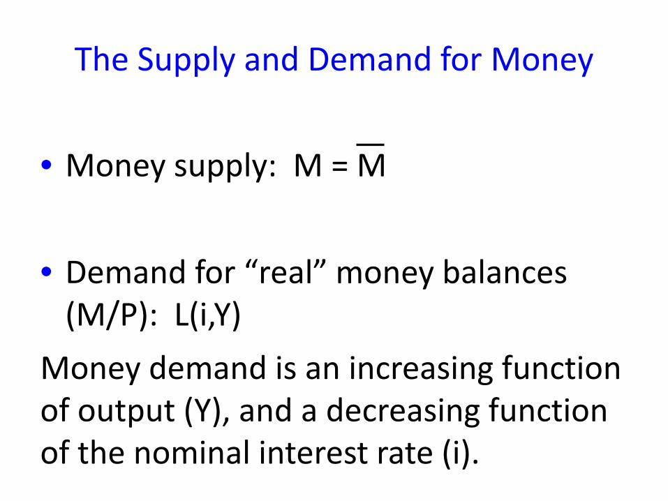
The Supply and Demand for Money • Money supply: M = M • Demand for “real” money balances

(M/P): L(i,Y) Money demand is an increasing function of output (Y), and a decreasing function of the nominal interest rate (i).

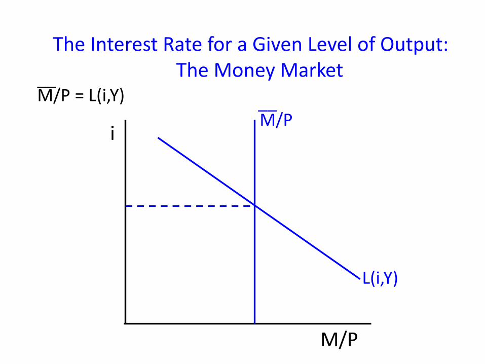
The Interest Rate for a Given Level of Output: The Money Market

M/P = L(i,Y)

M/P

i

__

L(i,Y)

M/P __

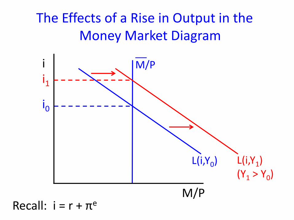
The Effects of a Rise in Output in the Money Market Diagram

Recall: i = r + πe M/P

i

i0

M/P

L(i,Y0)

__

L(i,Y1) (Y1 > Y0)

i1

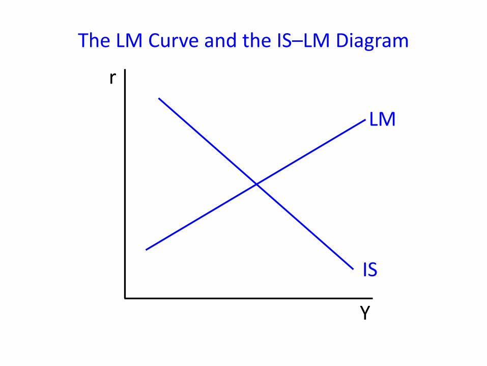
The LM Curve and the IS–LM Diagram

Y

r

IS

LM

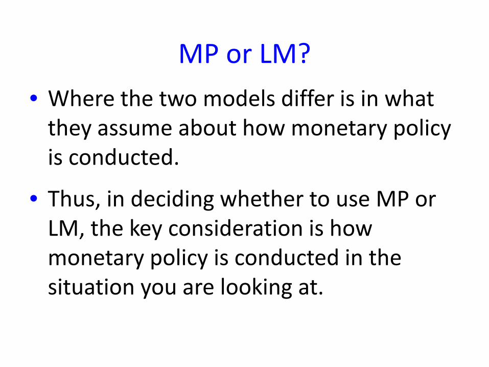
MP or LM? • Where the two models differ is in what

they assume about how monetary policy is conducted.

• Thus, in deciding whether to use MP or LM, the key consideration is how monetary policy is conducted in the situation you are looking at.

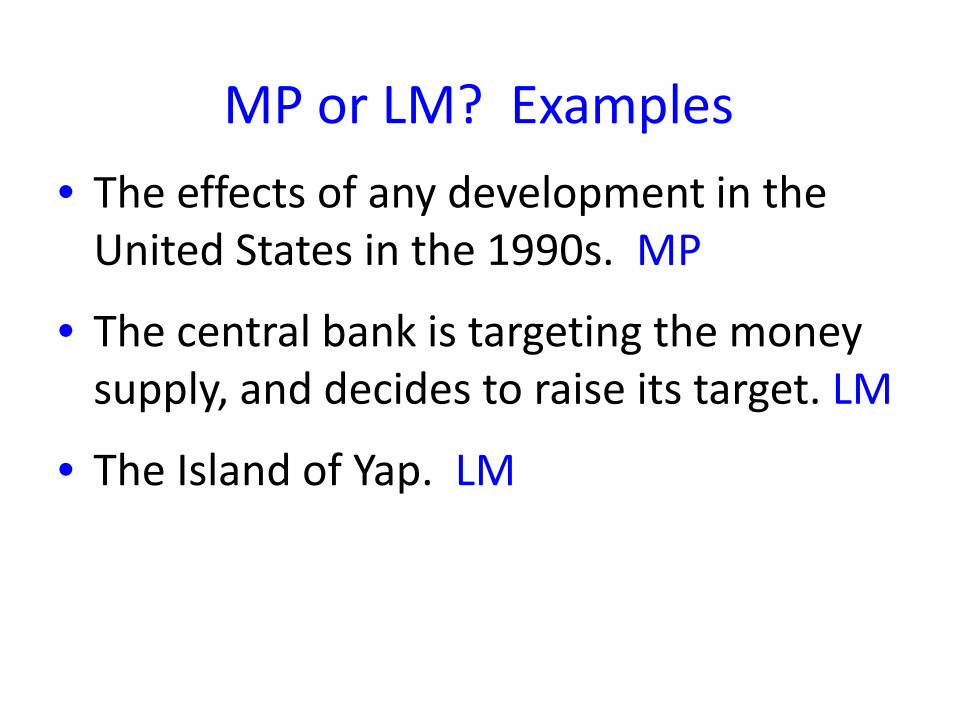
MP or LM? Examples • The effects of any development in the

United States in the 1990s. MP

• The central bank is targeting the money supply, and decides to raise its target. LM

• The Island of Yap. LM

II. EXAMPLES

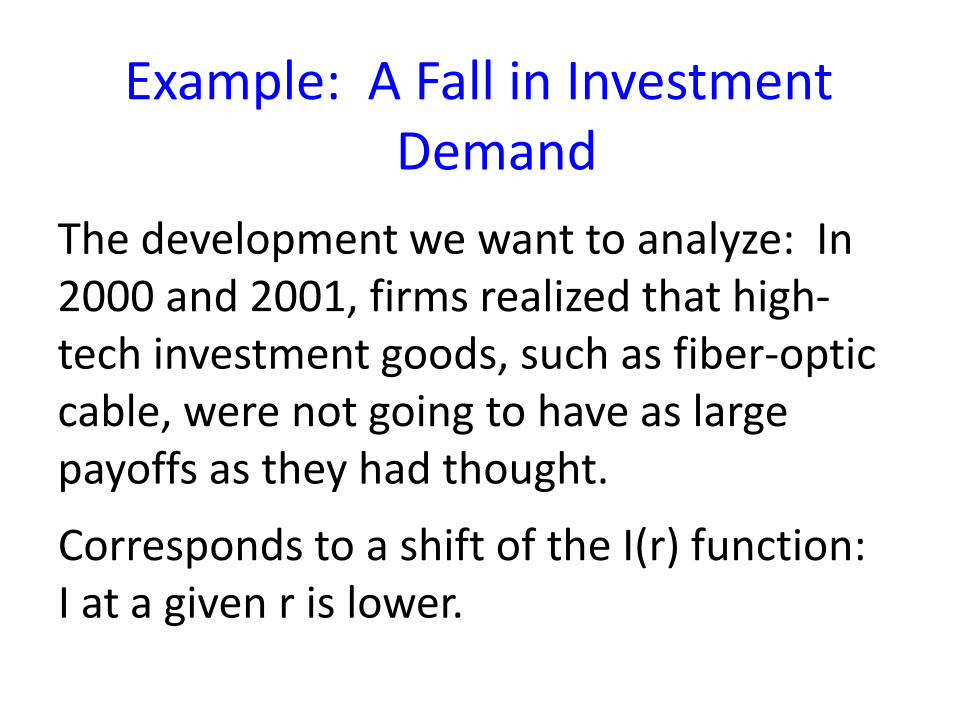
Example: A Fall in Investment Demand

The development we want to analyze: In 2000 and 2001, firms realized that high-tech investment goods, such as fiber-optic cable, were not going to have as large payoffs as they had thought.

Corresponds to a shift of the I(r) function: I at a given r is lower.

MP or LM? MP

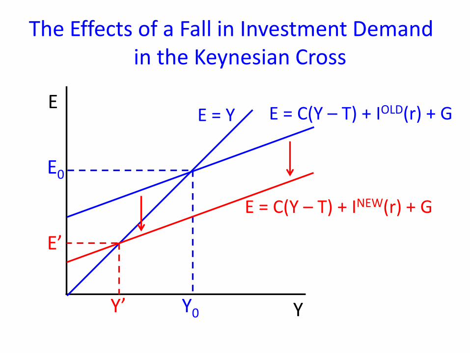
The Effects of a Fall in Investment Demand in the Keynesian Cross

Y

E E = Y E = C(Y – T) + IOLD(r) + G

E0

Y0

E = C(Y – T) + INEW(r) + G

Y’

E’

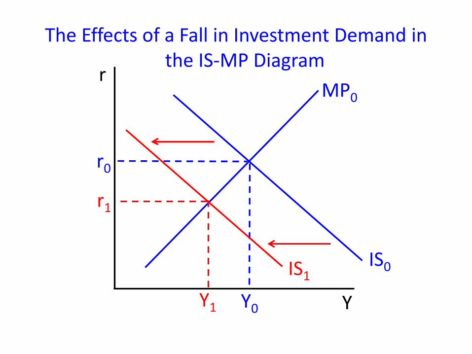
The Effects of a Fall in Investment Demand in the IS-MP Diagram

Y

r MP0

IS0

r0

Y0 IS1

Y1

r1

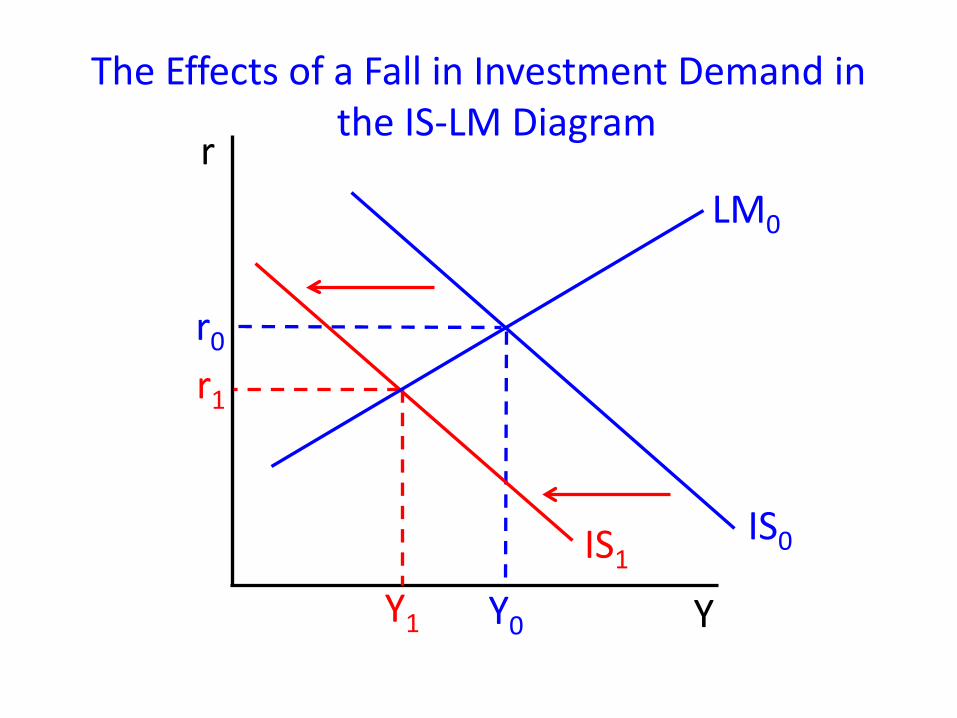
The Effects of a Fall in Investment Demand in the IS-LM Diagram

Y

r LM0

IS0

r0

Y0 IS1

Y1

r1

Example: Financial Innovation

The development we want to analyze: New technologies allow people to make many purchases using debit cards that they used to have to make using cash.

Corresponds to a shift of the L(i,Y) function: money demand at a given i and Y is lower.

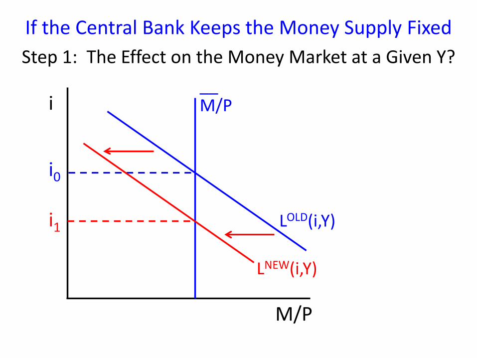
If the Central Bank Keeps the Money Supply Fixed Step 1: The Effect on the Money Market at a Given Y?

M/P

i

i0

M/P

LOLD(i,Y)

__

LNEW(i,Y)

i1

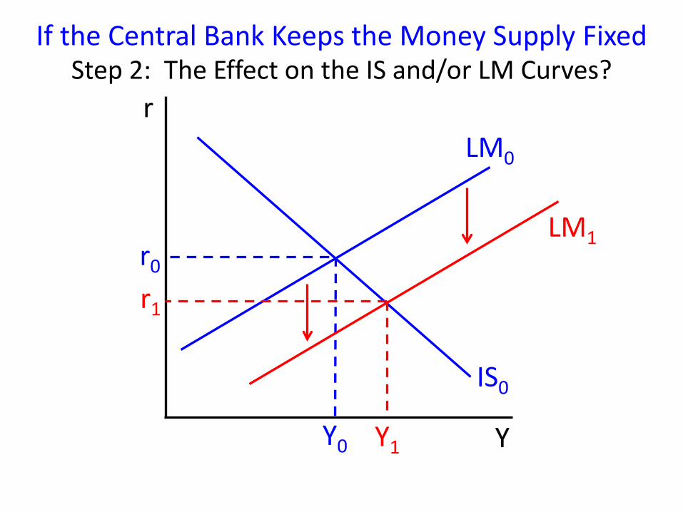
If the Central Bank Keeps the Money Supply Fixed Step 2: The Effect on the IS and/or LM Curves?

Y

r LM0

IS0

r0

Y0

LM1

r1

Y1

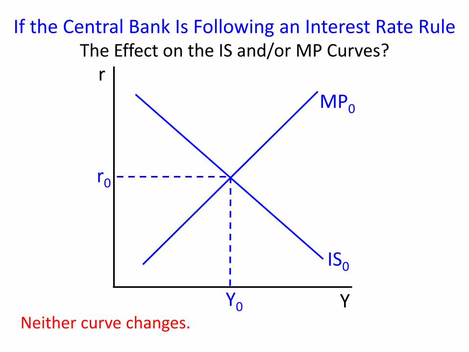
If the Central Bank Is Following an Interest Rate Rule The Effect on the IS and/or MP Curves?

Y

r MP0

IS0

r0

Y0 Neither curve changes.

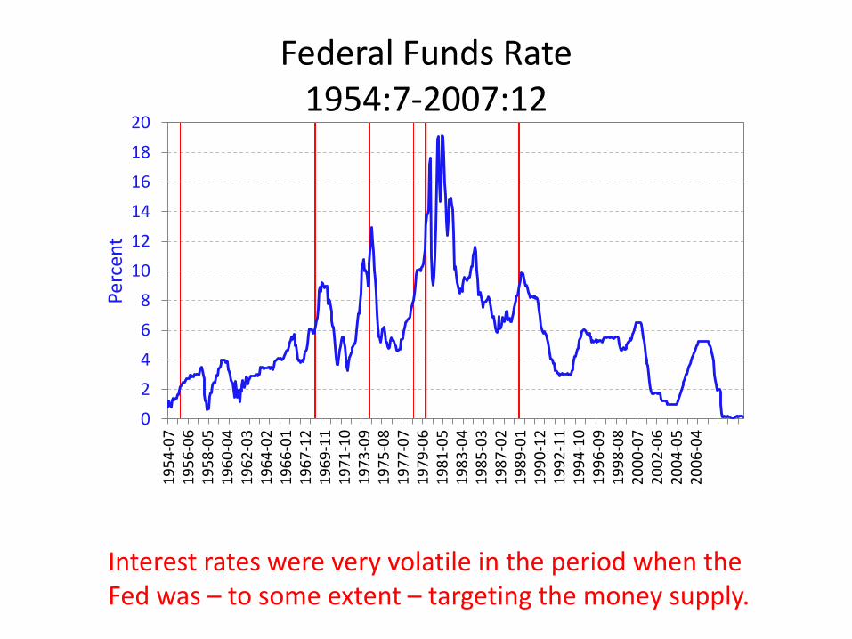
Interest rates were very volatile in the period when the Fed was – to some extent – targeting the money supply.

02468

101214161820

1954

-07

1956

-06

1958

-05

1960

-04

1962

-03

1964

-02

1966

-01

1967

-12

1969

-11

1971

-10

1973

-09

1975

-08

1977

-07

1979

-06

1981

-05

1983

-04

1985

-03

1987

-02

1989

-01

1990

-12

1992

-11

1994

-10

1996

-09

1998

-08

2000

-07

2002

-06

2004

-05

2006

-04

Perc

ent

Federal Funds Rate 1954:7-2007:12