Head into the Cloud: An Analysis of the Emerging Cloud

Head into the Cloud: An Analysis of theEmerging Cloud Infrastructure

by

Balakrishnan Chandrasekaran

Department of Computer ScienceDuke University

Date:Approved:

Bruce M. Maggs, Supervisor

Theophilus A. Benson

Jeffrey S. Chase

Landon P. Cox

Walter Willinger

Dissertation submitted in partial fulfillment of the requirements for the degree ofDoctor of Philosophy in the Department of Computer Science

in the Graduate School of Duke University2016

ABSTRACT

Head into the Cloud: An Analysis of the EmergingCloud Infrastructure

by

Balakrishnan Chandrasekaran

Department of Computer ScienceDuke University

Date:Approved:

Bruce M. Maggs, Supervisor

Theophilus A. Benson

Jeffrey S. Chase

Landon P. Cox

Walter Willinger

An abstract of a dissertation submitted in partial fulfillment of the requirementsfor

the degree of Doctor of Philosophy in the Department of Computer Sciencein the Graduate School of Duke University

2016

Copyright c© 2016 by Balakrishnan ChandrasekaranAll rights reserved except the rights granted by the

Creative Commons Attribution-Noncommercial Licence

http://creativecommons.org/licenses/by-nc/3.0/us/

Abstract

We are witnessing a paradigm shift in computing—people are increasingly using

Web-based software for tasks that only a few years ago were carried out using

software running locally on their computers. The increasing use of mobile de-

vices, which typically have limited processing power, is catalyzing the idea of

offloading computations to the cloud. It is within this context of cloud computing

that this thesis attempts to address a few key questions: (a) With more computa-

tions moving to the cloud, what is the state of the Internet’s core? In particular, do

routing changes and consistent congestion in the Internet’s core affect end users’

experiences? (b) With software-defined networking (SDN) principles increasingly

being used to manage cloud infrastructures, are the software solutions robust (i.e.,

resilient to bugs)? With service outage costs being prohibitively expensive, how

can we support network operators in experimenting with novel ideas without

crashing their SDN ecosystems? (c) How can we build a large-scale passive IP

geolocation system to geolocate the entire IP address space at once so that cloud-

based software can utilize the geolocation database in enhancing the end-user

experience? (d) Why is the Internet so slow? Since a low-latency network allows

more offloading of computations to the cloud, how can we reduce the latency in

the Internet?

iv

v

Contents

Abstract iv

List of Tables xi

List of Figures xii

List of Abbreviations and Symbols xvi

Acknowledgements xvii

1 Introduction 1

1.1 Motivation . . . . . . . . . . . . . . . . . . . . . . . . . . . . . . . . . 2

1.2 Contributions . . . . . . . . . . . . . . . . . . . . . . . . . . . . . . . 4

1.2.1 Ramifications of Cloud Computing . . . . . . . . . . . . . . 5

1.2.2 Management of Cloud Infrastructure . . . . . . . . . . . . . 6

1.2.3 Leveraging the Cloud . . . . . . . . . . . . . . . . . . . . . . 7

1.2.4 Supporting the Cloud-Computing Model . . . . . . . . . . . 8

1.3 Organization . . . . . . . . . . . . . . . . . . . . . . . . . . . . . . . . 9

2 A Server-to-Server View of the Internet 11

2.1 Challenges . . . . . . . . . . . . . . . . . . . . . . . . . . . . . . . . . 12

2.2 Contributions . . . . . . . . . . . . . . . . . . . . . . . . . . . . . . . 14

2.3 Acknowledgments . . . . . . . . . . . . . . . . . . . . . . . . . . . . 16

2.4 Data Sets . . . . . . . . . . . . . . . . . . . . . . . . . . . . . . . . . . 16

2.4.1 Server Logs . . . . . . . . . . . . . . . . . . . . . . . . . . . . 17

vi

2.4.2 Long-term Measurements . . . . . . . . . . . . . . . . . . . . 18

2.4.3 Short-term Measurements . . . . . . . . . . . . . . . . . . . . 20

2.5 Back-Office Traffic . . . . . . . . . . . . . . . . . . . . . . . . . . . . . 21

2.5.1 Front-office vs. back-office CDN traffic . . . . . . . . . . . . 21

2.5.2 Traffic Characteristics . . . . . . . . . . . . . . . . . . . . . . 24

2.6 Server-to-Server Path Measurements: An Illustrative Example . . . 25

2.7 Impact of Routing Changes . . . . . . . . . . . . . . . . . . . . . . . 28

2.7.1 Methodology for Inferring Changes . . . . . . . . . . . . . . 28

2.7.2 Data Trends over Long-term . . . . . . . . . . . . . . . . . . 30

2.7.3 Data Trends over Short-term . . . . . . . . . . . . . . . . . . 36

2.8 Impact of Congestion . . . . . . . . . . . . . . . . . . . . . . . . . . . 38

2.8.1 Is Congestion the Norm in the Core? . . . . . . . . . . . . . . 38

2.8.2 Locating Congestion . . . . . . . . . . . . . . . . . . . . . . . 39

2.8.3 Identifying Router Ownership . . . . . . . . . . . . . . . . . 41

2.8.4 Estimating Congestion Overhead . . . . . . . . . . . . . . . . 44

2.9 IPv4 vs IPv6 . . . . . . . . . . . . . . . . . . . . . . . . . . . . . . . . 46

2.10 Discussion . . . . . . . . . . . . . . . . . . . . . . . . . . . . . . . . . 48

2.11 Summary . . . . . . . . . . . . . . . . . . . . . . . . . . . . . . . . . . 50

3 Failures as a First-class Citizen 52


3.2 Motivation . . . . . . . . . . . . . . . . . . . . . . . . . . . . . . . . . 57

3.2.1 State of the SDN Ecosystem . . . . . . . . . . . . . . . . . . . 57

3.2.2 SDN-App Failure Scenarios . . . . . . . . . . . . . . . . . . . 59

3.2.3 Implications of SDN-App Failures . . . . . . . . . . . . . . . 60

3.2.4 Challenges in Crash Recovery . . . . . . . . . . . . . . . . . 61

vii

3.2.5 Design Goals . . . . . . . . . . . . . . . . . . . . . . . . . . . 62

3.3 System Architecture . . . . . . . . . . . . . . . . . . . . . . . . . . . . 64

3.4 Cross-Layer Transactions . . . . . . . . . . . . . . . . . . . . . . . . . 68

3.4.1 Snapshots . . . . . . . . . . . . . . . . . . . . . . . . . . . . . 69

3.4.2 Rollbacks . . . . . . . . . . . . . . . . . . . . . . . . . . . . . 70

3.4.3 Maintaining Consistency . . . . . . . . . . . . . . . . . . . . 71

3.5 Event Transformations . . . . . . . . . . . . . . . . . . . . . . . . . . 73

3.6 Prototype . . . . . . . . . . . . . . . . . . . . . . . . . . . . . . . . . . 77

3.7 Evaluation . . . . . . . . . . . . . . . . . . . . . . . . . . . . . . . . . 78

3.7.1 Experimental Setup . . . . . . . . . . . . . . . . . . . . . . . . 79

3.7.2 Recovery Time . . . . . . . . . . . . . . . . . . . . . . . . . . 80

3.7.3 Event Transformations . . . . . . . . . . . . . . . . . . . . . . 83

3.7.4 Application State Recovery . . . . . . . . . . . . . . . . . . . 85

3.7.5 Cross-layer Transaction Support . . . . . . . . . . . . . . . . 86

3.8 Related Work . . . . . . . . . . . . . . . . . . . . . . . . . . . . . . . 87

3.9 Discussion . . . . . . . . . . . . . . . . . . . . . . . . . . . . . . . . . 88

3.10 Summary . . . . . . . . . . . . . . . . . . . . . . . . . . . . . . . . . . 90

4 Alidade: Passive IP Geolocation 91

4.1 Contributions . . . . . . . . . . . . . . . . . . . . . . . . . . . . . . . 93


4.3 Related Work . . . . . . . . . . . . . . . . . . . . . . . . . . . . . . . 96

4.3.1 Active Approaches . . . . . . . . . . . . . . . . . . . . . . . . 97

4.3.2 Passive Approaches . . . . . . . . . . . . . . . . . . . . . . . 101

4.4 System Design . . . . . . . . . . . . . . . . . . . . . . . . . . . . . . . 103

4.4.1 Preprocessor . . . . . . . . . . . . . . . . . . . . . . . . . . . . 103

viii

4.4.2 Iterative Solver . . . . . . . . . . . . . . . . . . . . . . . . . . 106

4.4.3 Extrapolator . . . . . . . . . . . . . . . . . . . . . . . . . . . . 108

4.4.4 Preloader . . . . . . . . . . . . . . . . . . . . . . . . . . . . . 109

4.4.5 Aggregator . . . . . . . . . . . . . . . . . . . . . . . . . . . . 109

4.4.6 Query Engine . . . . . . . . . . . . . . . . . . . . . . . . . . . 110

4.4.7 Exploiting Registry Data . . . . . . . . . . . . . . . . . . . . . 112

4.4.8 Matching City Names to Shapes . . . . . . . . . . . . . . . . 113

4.4.9 Additional Shape Sets . . . . . . . . . . . . . . . . . . . . . . 115

4.5 Evaluation . . . . . . . . . . . . . . . . . . . . . . . . . . . . . . . . . 115

4.5.1 Ground-truth Data . . . . . . . . . . . . . . . . . . . . . . . . 116

4.5.2 Experimental Setup . . . . . . . . . . . . . . . . . . . . . . . . 117

4.5.3 Comparative Evaluation Results . . . . . . . . . . . . . . . . 119

4.5.4 Lessons Learned . . . . . . . . . . . . . . . . . . . . . . . . . 124

4.6 Summary . . . . . . . . . . . . . . . . . . . . . . . . . . . . . . . . . . 126

5 The Internet at the Speed of Light 128


5.2 The Need for Speed . . . . . . . . . . . . . . . . . . . . . . . . . . . . 130

5.3 The Internet is too slow . . . . . . . . . . . . . . . . . . . . . . . . . . 133

5.3.1 PlanetLab Measurements . . . . . . . . . . . . . . . . . . . . 133

5.3.2 Client connections to a CDN . . . . . . . . . . . . . . . . . . 135

5.3.3 RIPE Atlas Measurements . . . . . . . . . . . . . . . . . . . . 138

5.4 Case Study: Faster Page Loads . . . . . . . . . . . . . . . . . . . . . 141

5.5 Related Work . . . . . . . . . . . . . . . . . . . . . . . . . . . . . . . 144

5.6 Summary . . . . . . . . . . . . . . . . . . . . . . . . . . . . . . . . . . 145

ix

6 Roadmap 147

6.1 Dissecting End-User Experience . . . . . . . . . . . . . . . . . . . . . 147

6.2 On IPv4-IPv6 Infrastructure Sharing . . . . . . . . . . . . . . . . . . 150

6.3 Towards a Speedier Internet . . . . . . . . . . . . . . . . . . . . . . . 151

7 Conclusion 152

Bibliography 154

Biography 175

x

List of Tables

2.1 Summary of traceroutes (in millions) collected between dual-stack servers 19

3.1 Brief list of SDN-Apps showcasing the rich diversity in the SDN ecosys-tem: many SDN-Apps come from third-party software vendors . . . . . . 58

3.2 State-changing control messages and their inverses. . . . . . . . . . . . . 70

3.3 Sample list of event transformations in LegoSDN. . . . . . . . . . . . . . 74

4.1 Unique IP addresses and geographic locations associated with the data setsused for evaluating geolocation databases . . . . . . . . . . . . . . . . . 116

4.2 Number of targets in the different data sets with delay-based measurementdata (for geolocation) . . . . . . . . . . . . . . . . . . . . . . . . . . . . 118

xi

List of Figures

2.1 A CDN’s perspective on back-office Web traffic volume . . . . . . . . . . 23

2.2 Fan out in different traffic categories: fan out in the back-office categoriesis two orders of magnitude smaller than that in the front-office (CDN-EndUsers) category. . . . . . . . . . . . . . . . . . . . . . . . . . . . . 24

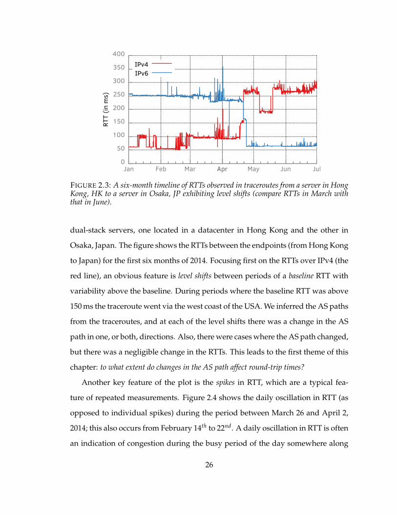
2.3 A six-month timeline of RTTs observed in traceroutes from a server inHong Kong, HK to a server in Osaka, JP exhibiting level shifts (compareRTTs in March with that in June). . . . . . . . . . . . . . . . . . . . . . 26

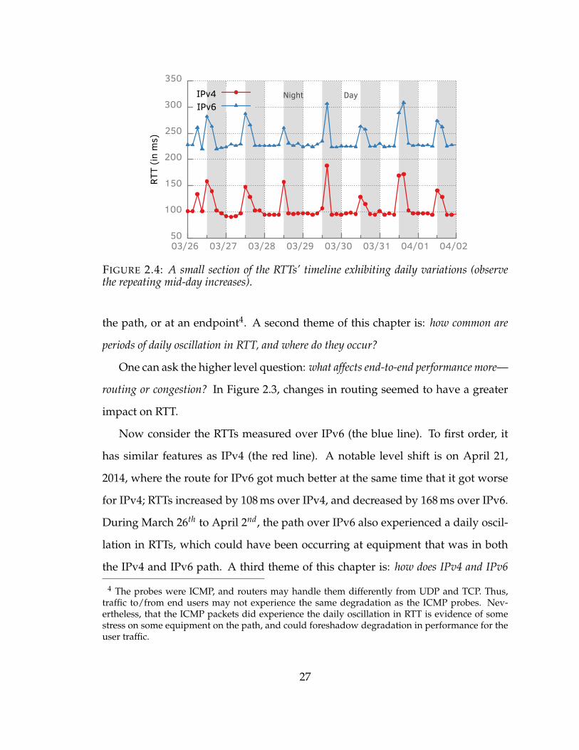
2.4 A small section of the RTTs’ timeline exhibiting daily variations (observethe repeating mid-day increases). . . . . . . . . . . . . . . . . . . . . . . 27

2.5 Number of unique AS paths and AS-path pairs observed in the 16-monthstudy period . . . . . . . . . . . . . . . . . . . . . . . . . . . . . . . . . 30

2.6 Frequency of routing changes and prevalence of popular AS paths over thecourse of 16 months . . . . . . . . . . . . . . . . . . . . . . . . . . . . . 31

2.7 Comparing magnitudes of increase in (baseline) 10th percentile of RTTsof AS paths (each relative to the best AS path of the corresponding tracetimeline) with the lifetime of AS paths. Sub-optimal AS paths with signif-icantly higher RTTs (top rows) are often short-lived (left-most columns).Suffixes ‘h’, ‘M’, and ‘D’ imply ‘hours’, ‘months’ and ‘days’. . . . . . . . 33

2.8 Comparing magnitudes of increase in 90th percentile of RTTs of AS paths(each relative to the best AS path of the corresponding trace timeline) withthe lifetime of AS paths. As the lifetime of AS paths increases the likeli-hood of the paths being sub-optimal (not offering the lowest 90th percentileof RTT compared to other paths between the corresponding server pair) de-creases. Suffixes ‘h’, ‘M’, and ‘D’ imply ‘hours’, ‘months’ and ‘days’. . . 35

2.9 Sub-optimal AS paths: approximately 1% of trace timelines over IPv4and 2% over IPv6 experienced at least a 100 ms increase in RTT becauseof sub-optimal AS paths with prevalence of 20% or more. . . . . . . . . . 36

xii

2.10 Comparing magnitudes of increase in the (a) 10th, and (b) 90th percentilesof RTTs of AS paths (each relative to the “best” AS path of the correspond-ing trace timeline) in the short-term data set. Results using traceroutesconducted 3 hours apart (lines with suffix ‘3hr’) are not different from thatusing traceroutes done 30 minutes apart (lines with suffix ‘All’). . . . . . 37

2.11 Router ownership inference heuristics used on traceroutes to label in-terfaces observed with possible owners. The interfaces being labeled areshown in red and noted with a black dot. . . . . . . . . . . . . . . . . . . 42

2.12 Density of the congestion overhead in our data set . . . . . . . . . . . . . 45

2.13 Comparison end-to-end RTTs and inflation in RTTs over IPv4 with thoseover IPv6 . . . . . . . . . . . . . . . . . . . . . . . . . . . . . . . . . . 46

3.1 Normal and failure scenarios of an SDN-App setting up a flow path viaconfiguration of flow tables at three network switches. . . . . . . . . . . . 61

3.2 Comparison of LegoSDN architecture with the current SDN controllerarchitectures. . . . . . . . . . . . . . . . . . . . . . . . . . . . . . . . . 65

3.3 Timeline of transactions delimited by checkpoints . . . . . . . . . . . . . 66

3.4 Control and data flow schematic in LegoSDN . . . . . . . . . . . . . . . 67

3.5 Data-plane conflicts that may arise during failure recovery. . . . . . . . . 72

3.6 Hierarchy of Event Transformations. . . . . . . . . . . . . . . . . . . . . 76

3.7 Comparison of different recovery techniques and analysis of time spent indifferent recovery functions . . . . . . . . . . . . . . . . . . . . . . . . . 81

3.8 Experimental setup for evaluating the use of event transformations. . . . 83

3.9 Safe SDN-App recovery from deterministic and non-deterministic faults . 84

4.1 Example of a geolocation prediction made by Alidade for a target. . . . . . 94

4.2 Alidade system pipeline and its components . . . . . . . . . . . . . . . . 103

4.3 CDF of iPlane traceroute measurements violating speed-of-light constraints104

4.4 Direct and indirect observations obtained from delay-based measurements 106

4.5 Use of direct and indirect constraints in making a geolocation predictionfor a target . . . . . . . . . . . . . . . . . . . . . . . . . . . . . . . . . . 107

xiii

4.6 Alidade’s extrapolator guessing the locations of targets in the tail end of atrace path . . . . . . . . . . . . . . . . . . . . . . . . . . . . . . . . . . 108

4.7 Example output from Alidade’s query engine showing the exact sequenceof steps followed by the system to make a geolocation prediction . . . . . . 111

4.8 Simplifying shape files (or reducing vertex count of shape polygons) usingthe α-shape algorithm . . . . . . . . . . . . . . . . . . . . . . . . . . . . 114

4.9 Accuracy of a naïve geolocation approach using Registry and HostParserhints, but no delay-based measurements . . . . . . . . . . . . . . . . . . 120

4.10 Comparison of Alidade’s geolocation accuracy with that of other geoloca-tion databases in the PLAB and MLAB data sets . . . . . . . . . . . . . 121

4.11 Comparison of Alidade’s geolocation accuracy with that of other geoloca-tion databases in the Ark and GPS data sets . . . . . . . . . . . . . . . . 122

4.12 Comparison of Alidade’s geolocation accuracy with that of other geoloca-tion databases in the NTP and EuroGT data sets . . . . . . . . . . . . . 123

4.13 Impact of temporal mismatch between Alidade’s inputs and ground-truthdata. . . . . . . . . . . . . . . . . . . . . . . . . . . . . . . . . . . . . . 124

4.14 Equivalent circle radii of Alidade’s predictions for 500 million IP addressesand ECDF of IP addresses whose predictions lie outside of Alidade’s pre-dictions . . . . . . . . . . . . . . . . . . . . . . . . . . . . . . . . . . . 125

5.1 Fetch time of just the HTML of the landing pages of popular Web sites interms of inflation over the speed of light. . . . . . . . . . . . . . . . . . . 134

5.2 Latency inflation in RTTs between end users and Akamai servers, and thevariation therein. . . . . . . . . . . . . . . . . . . . . . . . . . . . . . . 135

5.3 Variations in latencies of client-server pairs grouped into 2-hr windows indifferent geographic regions . . . . . . . . . . . . . . . . . . . . . . . . . 136

5.4 Medians of maximum change in RTTs (max - min) in repeat measure-ments within each time window. . . . . . . . . . . . . . . . . . . . . . . 137

5.5 Inflations in min. pings between RIPE Atlas nodes over both IPv4 and IPv6139

5.6 Inflation in minimum pings between RIPE Atlas nodes as a function ofc-latency . . . . . . . . . . . . . . . . . . . . . . . . . . . . . . . . . . . 140

5.7 Relative decrease in PLTs as underlying network latency is reduced . . . . 142

xiv

5.8 Relative decrease in PLTs as underlying network latency is reduced onlyalong the client-to-server direction . . . . . . . . . . . . . . . . . . . . . 143

6.1 Distribution of time spent in different phases involved in fetching Webobjects . . . . . . . . . . . . . . . . . . . . . . . . . . . . . . . . . . . . 148

xv

List of Abbreviations and Symbols

Abbreviations

AS Autonomous system.

ASN Autonomous system number.

BGP Border Gateway Protocol.

CDN Content delivery network.

DNS Domain Name System.

HDFS Hadoop Distributed File System.

IANA Internet Assigned Numbers Authority.

IXP Internet exchange point.

JVM Java Virtual Machine.

MPLS Multiprotocol Label Switching.

PLT Page load time.

RPC Remote procedure call.

RTT Round-trip time.

SDN Software-defined networking.

SDN-App Software-defined networking application.

SLA Service-level agreement.

xvi

Acknowledgements

It has been an enormous privilege to pursue my PhD at Duke University and a

humbling experience to be advised by Dr. Bruce MacDowell Maggs. There are

so many people to whom I am very grateful for their motivation, support and

guidance, and I apologize to those whom I may have forgotten to explicitly thank.

I am immensely grateful to Landon Cox, Jeff Chase, Theo Benson and Wal-

ter Willinger for serving on my committee and providing invaluable feedback.

Working with Theo was truly amazing: he is a great mentor, and a very optimistic

researcher. His polite way of pointing out mistakes and generosity in acknowl-

edging even modest contributions of others are traits I hope to imbibe. There’s

also nothing more comforting than hearing encouraging words about my research

from Walter; his crisp and clear critiquing style, and modesty are attributes that I

intend to shamelessly copy.

Sailesh Kumar, George Varghese and Jonathan Turner gave me my first taste

of doing academic research; am grateful to them for that incredible experience.

My research has benefitted immensely from collaborations with so many amaz-

ing folks—Ankit Singla, Brighten Godfrey, Phillip Richter, Enric Pujol, Anja Feld-

mann, Reza Rejaie, Reza Motamedi, Sanjay Rao, Shankaranarayanan Narayanan,

Ashiwan Sivakumar, He Yan, Ge Zihui, Aman Sheikh, Nicholas Duffield, Arthur

Berger, K.C. Ng, Georgios Smaragdakis, Kyle Moses, Michael Schoenfield, Min-

gru Bai, David Duff, Richard Weber, Matt Olson, Keith Jordy, Jan Galkowski,

xvii

David Plonka, Steve Hoey, John Thompson, George Economou, Bernard Wong,

and Emin Gün Sirer. Brighten’s attention to detail and Anja’s ability to succinctly

express an idea have greatly influenced my writing style. It took me three years to

convince Arthur to collaborate with me, and I would have tried even harder had

I known how much fun I would have working with him. I thank Georgios for his

motivation and guidance; there was never a dull moment (or a sober one) when

he was around. If not for David’s confidence in me and Rick’s patience, it would

have been impossible to intern at Akamai for three summers. I am also deeply

indebted to K.C. for teaching me how to be a patient researcher, a good developer

and a better human being.

I thank profusely the Duke staff and colleagues for the engaging hallway dis-

cussions (especially the ones at ungodly hours), and, in general, for making my

time at Duke a memorable one. I am also lucky for having Janardhan Kulkarni,

Nedyalko Borisov, Reza Motamedi and Brendan Tschaen as friends—thanks for

being brutally honest in critiquing my work. I will never know how to thank

Marilyn Butler for her comforting words or the herb bouquet. Victor Orlikowski,

Herodotus Herodotou, Eduardo Cuervo, Amre Shakimov, Yu chen, Rohit Par-

avastu, Bing Xie, Rishi Thonanghi, Vamsidhar Thummala, Qiang Cao, Ali Razeen,

Botong Huang, Yezhou Huang, Dina Hafez, Alan Davidson, Jannie Tan, Xiaom-

ing Xu, Ilker Bozkurt, Animesh Srivastava, Mayuresh Kunjir, Alex Meijer, Nisarg

Raval—my graduate life wouldn’t be the same without you.

I spent a few years working as a software developer prior to coming to Duke.

While the decision to go back to graduate school was one of my best decisions

so far, I was very scared at that time. I am thankful to the people who stood by

my side and encouraged me to go to Duke: George Hunter, Meenakshi Sharma,

Badri Vishal Dwivedi, Fred Kuhns, Anand Prasanna Venkatesan, Chandramouli

Shankaranarayanan, Kishor Kadu, Ravi Tanniru, Suchith Hegde, Thanigainathan

xviii

Manivannan, Sriram Srinivasan, Arvind Ravichandran, Bhuvaneswari Ramku-

mar, and Charanya Venkatraman, and Sivaraj Palaniswamy. If I am a better de-

veloper today, it is because of the freedom I had in developing software under

George.

I owe a lot to Rozemary Scarlat, my best friend and soul mate, for her en-

couragement and support, and for always being there to listen to my ramblings.

I thank my parents, godparents, sister and relatives for their unconditional love

and affection. I didn’t realize for much of my childhood that I grew up in a poor

family and for that I thank my dad. But it was my mom who never missed an

opportunity to stress the importance of education and wholeheartedly supported

me in all my endeavors. It is hard to repay the kindness of my uncles Usman

and Pauly, and even unimaginable to think of that of my aunt Hemalatha. Lastly,

I thank my uncle Balaji for his support and encouragement; he will always be a

great source of inspiration.

I have never been certain of anything other than that I will fail miserably in

expressing my gratitude to Bruce, my adviser. In a way, Bruce worked harder

than I, during the last six years, to make me better in every facet of my professional

and personal life. It is unbelievable to realize that my adviser has made me laugh

more than anyone else. Bruce never passed a chance to make fun of me, but it

is incredible that he chose to make me laugh at my mistakes than let me worry

about them. His extraordinary patience when it comes to tolerating my crash-

prone software, outrageous ideas, and ill-conceived jokes is astounding and one

that was key to my survival at Duke. Had it not been for Bruce, I am sure I would

not have come this far, and I will try to continue justifying the opportunity that he

gave me.

xix

1

Introduction

Nothing endures but change

— Heraclitus of EphesusGreek Philosopher

The Internet is inherently complex and is constantly evolving. Indeed, a re-

markable achievement of computer scientists is in taming the Internet’s complex-

ity in three simple words: its definition that the Internet is simply a “network of

networks”. Abstraction is the community’s forte, after all. While staying com-

pliant to this abstraction for over half a century since its inception, the Internet

has undergone massive changes, spanning the spectrum from the elegant and in-

evitable to the surprising and unexpected. The evolution in the protocols and

techniques used for addressing hosts (or loosely, computers) in the Internet—from

a manually maintained ledger of 32-bit addresses to an elegant decentralized reg-

istration scheme of addresses drawn from a massive 128-bit space—makes for an

interesting testimony (or a story) showcasing one of the many transformations of

the Internet.

People are increasingly using Web-based software for tasks which only a few

years ago were carried out using software running locally on their computers.

1

Sometimes the lines between “local” and “remote” computations are intentionally

(and successfully) blurred, and we take for granted that the Internet is intertwined

in almost every task we carry out, whether it is in our desktops, laptops, or mobile

devices. This idea of delivering software as services over the Internet, or cloud—in

essence, performing computations on remote machines and retrieving the results

over the Internet—is what we refer to as cloud computing. It may indeed be worth-

while to debate and attribute the origin of cloud computing to the “time sharing”

concept introduced by John McCarthy [144, 176], and trace its rise, fall and res-

urrection in its current form. As networking researchers, however, we digress

and focus instead, in this thesis, on analyzing the impact of cloud computing on

the Internet and identifying ways to enhance and support the cloud-computing

model.

1.1 Motivation

Whether it started as a means to share expensive resources among multiple users,

or came about as a feasible approach to manage inexpensive systems in a cost-

effective manner, cloud computing has garnered a lot of attention and endorse-

ments, in the form of investments. Google reported that revenues from their cloud

platform could surpass that from Google’s advertising; it is worth noting that 96%

of Google’s revenues are from advertising [121] and it’s advertising revenue is

over 15 billion dollars in any quarter [34, 33, 32]. Gartner’s report on technology

trends for 2015 [94] showed the pervasiveness of cloud computing; most, if not

all, of the technology trends included in the report relied on cloud computing, a

market that is expected to reach over 200 billion dollars in 2016 [95].

Technically, cloud computing encompasses three different models—Software as

a Service (SaaS), Infrastructure as a Service (IaaS), and Platform as a Service (PaaS)—

2

with the difference being in what is abstracted and delivered as a service to the

end users. The term ‘cloud’ is suggestive of the abstraction that masks from the

user from inferring the mechanism or implementation of the services or computa-

tions. In essence, users of the services are often unaware of whether the software

providing the services are running remotely. In this thesis, we do not differentiate

between the different cloud-computing models; the nuances of these models is

neither relevant to our work nor is a requirement for understanding this thesis.

The performance characteristics of the network pipes that bridge the gap be-

tween the local and remote parts, in the cloud computing paradigm, dictate the

experience of the users of the services. Poor performance, e.g., high latency, con-

gestion, in the Internet’s core could drastically affect the end-user experience. Nat-

urally, there is a need to measure and understand the state of the Internet core,

and identify opportunities for improvements. Running software in the cloud, in a

logically centralized location, still provides ample opportunities to individualize

services for each user, with monetization being a key incentive.

Much of the cloud computing infrastructure relies on software modules for

control and management. Software-defined networking (SDN) principles, for in-

stance, are increasingly being used to manage cloud infrastructures [131, 199]. The

SDN ecosystem boasts a thriving developer community providing innovative and

inexpensive, compared to the traditional style of network or infrastructure man-

agement, solutions; the ecosystem is still in its infancy. Automation of network

management can alleviate configuration errors and troubleshooting nightmares,

bugs are inevitable in software. Since the size of the user base of services running

in the cloud often runs into millions, the cloud amplifies the impact of crashes

induced by bugs in application managing the infrastructure. It is also hard to

monetize software that crashes on a personal computer, let alone one running in

the cloud and servicing millions of users. Consequently, it is crucial to understand

3

how robust SDN-based solutions are to bugs.

1.2 Contributions

It is within the context of cloud computing that this thesis attempts to address a

few key questions:

• With more computations moving to the cloud, what is the state of the In-

ternet’s core? In particular, do routing changes and consistent congestion in

the Internet’s core affect end users’ experience?

• With software-defined networking (SDN) principles increasingly being used

to manage cloud infrastructures, are the software solutions robust (i.e., re-

silient to bugs)? With service outage costs being prohibitively expensive,

how can we support network operators in experimenting with novel ideas

without crashing their SDN ecosystem?

• How can we build a large-scale passive IP geolocation system to geolocate

the entire IP address space at once so that cloud-based software can utilize

the geolocation database in enhancing the end-user experience?

• Why is the Internet so slow? Since a low-latency network allows more of-

floading of computations to the cloud, how can we cut down the latency in

the Internet?

More broadly, this thesis comprises of work along four dimensions: ramifi-

cations of cloud computing, management of cloud infrastructure, leveraging the

cloud, and supporting the cloud-computing model.

4

1.2.1 Ramifications of Cloud Computing

Today, delivering content to the end users involves a rich and complex interaction

between many servers. Advertisement objects, for instance, result from an on-

line bidding process involving several servers before these objects are delivered

to the end users. We identify a new class of Web traffic, referred to as back-office

Web traffic, that comprises only the data exchange occurring between servers. This

Web traffic, in other words, has servers being both its origin and destination; end

users are not involved in the data exchanges. We used measurements from mul-

tiple vantage points to reveal that back-office Web traffic represents a significant

fraction of the core Internet traffic [175].

The increase in server-to-server communications also has important perfor-

mance implications for the end users. Measuring and monitoring the performance

of server-to-server paths, hence, is critical to estimating the quality of experience

of end users, and consequently, to quantifying monetization of services over the

cloud. To this end, in collaboration with researchers at Akamai, MIT and CAIDA,

we gathered nearly 1.2 billion (traceroute and ping) measurements over both IPv4

and IPv6 between 646 servers of a content delivery network (CDN) located in di-

verse geographic locations and networks across a period of 16 months. We used

the server-to-server paths as a proxy for the Internet’s core and analyzed the im-

pact of routing changes and congestion on the end-to-end latencies [59].

Understanding the performance characteristics of the core is key to designing

software for the cloud. In this regard, our study offers a first look on the impact

of congestion and routing on latency in the core using an extensive data set of

measurements from servers in 70 different countries. Congestion in the core is not

a well-understood topic—some claim it to be the norm, some argue that it is only

prevalent at peak times, and some completely dismiss the notion of a congested

5

core. To gain insight, we looked for consistent congestion, defined as recurring daily

oscillations in round-trip times (RTTs), in our data set and showed that it is not

the norm in the core. We also demonstrated that even routing changes at the AS-

level do not typically affect the end-to-end latencies. We show that the core can

consistently offer good performance (lower latency), a performance characteristic

that is key to support the rich and complex interaction between servers. The study

also highlights opportunities for reducing the server-to-server path latencies us-

ing dual-stacked servers and these latency reductions, in turn, can improve the

end-users’ experiences.

1.2.2 Management of Cloud Infrastructure

Data centers deployed to run the software or, more generally, computations in the

cloud are increasingly managed by SDN-based software applications [131, 199,

113, 62]. With an emerging marketplace for SDN applications, e.g., HP’s SDN

App Store [18], Open Daylight consortium [16], network operators now have an

opportunity to mix and match SDN applications from a wide variety of vendors

and run them on their data center or enterprise networks.

The current SDN controller architectures, however, do not provide a conducive

environment for experimenting with third-party SDN applications or rapid pro-

totyping of novel ideas. Most controller architectures are monolithic in nature and

often, there is poor or no isolation between the SDN applications. Faults resulting

from bugs in any one component, hence, bring down the entire SDN stack result-

ing in loss of network control. Even if the applications are isolated in sandboxes,

controllers do not support cross-layer transactions that span both control (changes

in application and network state) and data (input message from the network that

effected the state changes) planes. As such, current controllers cannot guarantee

that a crashing SDN application will not leave the network in an inconsistent state.

6

To address this issue, we propose LegoSDN, a novel fault-tolerant design of an

SDN controller that is resilient to crashes of SDN applications [57]. We demon-

strate using a prototype implementation that LegoSDN can recover failed SDN

applications three times faster than controller reboots and can even transform a

crash-inducing message to a different but equivalent message (based on the Open-

Flow specification [163]) to recover from deterministic faults [60]. By making the

SDN controller resilient to crashes of SDN applications, LegoSDN encourages op-

erators to experiment with novel applications that can more efficiently monitor

and better utilize the network. A safer and efficient cloud in turn fosters more

offloading of computations to the cloud.

1.2.3 Leveraging the Cloud

Despite the fact that the cloud provides services for millions of users, with some

effort it is still possible to individualize the services for each user; not only are such

customized services desirable, they can be invaluable in monetizing the services.

In this regard, geolocating the IP addresses to infer the end-users’ locations offers

a promising first step towards providing customized services for the end users.

Although the IP geolocation problem has been studied extensively, the systems

discussed in academic literature have relied, typically, on active probing where the

system issues measurement probes to gather delay-based measurements required

for making the geolocation prediction. The task of geolocating the entire IPv4

address space, let alone IPv6, at once is infeasible using active probing. To address

the issue, we collaborated (along with researchers at Akamai, Cornell Universty

and University of Waterloo) in the design and development of Alidade, a passive IP

geolocation system [56].

Alidade is fundamentally different from all prior research systems since it

computes predictions for the entire IP address space while absolutely refraining

7

from issuing any measurement probes of its own, either before or after it is pre-

sented with the IP addresses. While geolocation systems relying on extensive use

of active probing often annoy both network operators and the targets probed, pas-

sive geolocation, by definition, is unobtrusive. Alidade’s geolocation prediction is

a polygonal feasible region that represents all possible locations of the IP address,

but the system also makes a point-based prediction for comparing its predictions

with that of the other geolocation systems. Alidade is designed as a map-reduce

application that can ingest a wide variety of measurement and non-measurement

data from both public and private data sets. Rather than treat a geolocation pre-

diction as an output from a black box, Alidade provides details on all inputs that

were available for making the prediction, including those that were not used in

the prediction. By exposing the internals of the algorithm used in making a pre-

diction, Alidade assists the user in making an informed choice on how to use the

prediction. The design choice potentially enables use of machine-learning tech-

niques to automatically explore the space of heuristics and determine better ways

of generating geolocation predictions. An accurate database of geolocation predic-

tions is an invaluable tool for mapping the Internet topology, which can provide

insights into improving the cloud ecosystem.

1.2.4 Supporting the Cloud-Computing Model

Latency is critical to the idea of running software in the cloud. A low-latency net-

work allows more computations to be offloaded to the cloud, while giving the end

users an illusion that they are running their computations locally (on their own

machines). The Internet, however, is shockingly slow! We collaborated with re-

searchers at the University of Illinois, Urbana Champaign to show that the median

time to fetch just the HTML documents of popular Web sites was 35-times slower

than the round-trip speed-of-light (cSpeed) latency (between the corresponding

8

clients and servers) [196]. Using the RIPE Atlas [148] measurement platform, we

reveal that inflation in minimum pings measured from the Internet’s edge is often

8-times or more compared to cSpeed latency. We analyzed possible sources of la-

tency and showed that infrastructural improvements alone could reduce latency

by at least a factor of three.

In a subsequent manuscript, we discussed the design of a parallel low-latency

Internet to connect the top cities in United States using microwave communica-

tions along straight-line paths and highlighted the incentives of having such a

parallel low-latency infrastructure [197]. We define page-load time (PLT) as the

time spent by a browser to completely load all the contents of a Web page, and

measure improvements in PLTs when utilizing a parallel low-latency infrastruc-

ture. We use a Web page record-and-replay toolkit to record the page data as well

as the RTTs of the network connections made by the Web browser while fetching

this Web page data, and replay these fetches over an emulated network with RTTs

lower than that originally measured; note that the contents fetched during the re-

play phase is identical to that fetched during the record phase. The measurement

of reductions in PLTs helps us quantify the benefits of latency reductions in terms

of its impact on end-user experience. To this end. we show a 30% reduction in

median PLT, which corresponds to an absolute reduction of 602 ms, when we can

reduce the network latency by 66%.

1.3 Organization

The rest of this thesis is organized as follows. Chapter 2 discusses our network

measurement effort to study the performance characteristics, viz., latency, con-

gestion, of the Internet’s core and identify opportunities to reduce the latency

in the core. Chapter 3 presents LegoSDN, a novel SDN controller architecture

9

that aims to treat failure as a first-class citizen. We discuss the motivations, sys-

tem design and conclude with comparative evaluation of LegoSDN against the

current state-of-the-art recovery techniques used with SDN stacks. We present

Alidade, a large-scale passive geolocation system in Chapter 4. In this chapter,

we compare Alidade’s geolocation accuracy with many commercial geolocation

databases, and highlight the details included with Alidade’s geolocation predic-

tions. We stress the issues in comparing geolocation databases and conclude with

a case-study to show how Alidade’s different and better than other commercial

offerings. Chapter 5 presents our findings on latency inflations in the Internet.

This chapter includes our analyses using Akamai’s data sets and measurements

performed using the RIPE Atlas platform. A summary of our research efforts is

included in Chapter 7, and we conclude with a brief discussion on future initia-

tives.

10

2

A Server-to-Server View of the Internet

One accurate measurement is worth a thousand expert opinions.— Grace Brewster M. Hopper

Inventor of the 1st programming language compiler

The Internet is massively heterogeneous and is continuously evolving, and no

single vantage point can, hence, capture the breadth of these changes [31]. To cut

the latency in delivering content to end users, CDNs have deployed massively dis-

tributed infrastructures and move content closer to end users. For cloud services,

the needs (for fresh content) and demands (for fast delivery) of a global user base

has forced data to be replicated and served from geographically distributed data-

centers. Consequently, the server-to-server landscape has transformed to support

these data delivery or cloud computing models; delivering data or results of com-

putations to end users involves a rich and complex interaction of many servers.

The network paths between the servers act as an excellent proxy to study the

Internet’s core: these paths capture the performance characteristics of the core

more than that of the other segments of the Internet. It is this server-to-server

view of the Internet that forms the central theme of this chapter. To understand

the complex interactions between servers, we capture and analyze logs, captur-

11

ing server-to-server data exchanges, from CDN servers. Our analysis indicates

that these interactions account for a significant fraction of the overall traffic vol-

ume and highlights one of the ramifications of serving data from and offloading

computations to the cloud. In this chapter, we highlight the insights gained into

the Internet’s core by conducting a longitudinal study of network measurements

over server-to-server paths. We discuss how routing changes and congestion in the

Internet’s core affect the end-users’ experience.

2.1 Challenges

There is a rich literature on edge-based (or end-user-based) network measurement

and mapping efforts. Such studies utilize vantage points at the Internet’s edge and

lend an end-user’s perspective on various aspects, e.g., performance of broadband

Internet [203], ISP bandwidth cap and throttling [79], performance of CDNs [209,

173], offloading services to the cloud [193, 81], and video streaming quality [21,

20, 80]. While the performance characteristics of access networks and end-user-

to-server paths are well-studied, measuring the performance of the Internet’s core

remains, largely, an uncharted territory.

A major obstacle to studying the state of the Internet’s core is the limited set

of vantage points to conduct accurate measurements and support such a study.

Looking glass servers, many of which are located at core routers, for instance, can

offer visibility into the core [123, 46]. They are, however, designed for testing basic

reachability and not measure end-to-end path performance. It is practically infea-

sible to collect bidirectional end-to-end measurements between two end points

using looking glass servers, let alone gathering such measurements periodically

and at scale. CDNs deploying massively distributed infrastructures closer to the

end user to deal with the pathologies of TCP implementations [130, 87], also po-

12

tentially limit the use of of end-user-based measurements to understand the state

of the core.

Although a number of measurement platforms, viz., PlanetLab [68], are avail-

able, their network coverage is limited: most of the measurement servers on these

platforms are installed in residential and academic networks. Other distributed

platforms viz., RIPE Atlas [148], are widely deployed and, hence, provide better

coverage. There are concerns, nevertheless, about the accuracy of delay-based

measurements obtained using such shared measurement platforms [111]. Cloud

servers are also known to be over-utilized and virtual machines can be trans-

parently migrated to different physical servers [132]; these are not good vantage

points for accurate delay-based measurements.

Studying the performance characteristics of router interconnections between

networks in the Internet’s core at scale would require the installation of thou-

sands of physical servers around the globe at a diverse set of peering locations

including colocation centers, datacenters, Internet exchange points (IXP), as well

as inside eyeball networks. While the idea of installing servers in a number of loca-

tions for Internet measurements is not new and has been shown to provide good

insights [169], it is prohibitively expensive to install servers in a large number of

peering locations and networks.

With more content being moved closer to the end-user, server-to-server paths

have increased in length and have a significant role in dictating the quality of

services offered by content and service providers. In this regard, we present a

large-scale longitudinal study of the effects of routing changes and congestion in

the Internet’s core on the end-to-end latencies of server-to-server paths. We also

measure the server-to-server Web traffic volume and discuss a few traffic charac-

teristics to highlight the ramifications of cloud computing.

13

2.2 Contributions

We broadly classify Internet Web traffic into two categories: front-office and back-

office Web traffic. Front-office Web traffic (or front-office traffic, in short) refers to

the traffic involving end users directly, e.g., traffic exchanged between end users

and CDN servers. In contrast, no end users are involved in the back-office Web

traffic (or back-office traffic, in short); the traffic refers to data exchanges between

only machines or servers, e.g., the data exchanged between the CDN servers at

different locations. We measure the back-office traffic volume by analyzing logs

obtained from servers of a CDN at multiple cities.

We investigate the state of the Internet’s core at scale: we exploit the dis-

tributed platform of a large content delivery network, composed of thousands

of servers around the globe, to assess the performance characteristics of the Inter-

net’s core. We routinely performed server-to-server measurements for more than

16 months, in both forward and reverse direction, and report on the state of the In-

ternet core from a service provider perspective. In particular, we study the affect

upon server-to-server round-trip times of (1) routing changes, and (2) significant

daily oscillations in latency, herein called congestion. Our work provides a com-

plementary view of the Internet at a scale that is currently difficult to obtain by

performing measurements at the edge of the Internet.

We summarize our contributions as follows.

• We show, using logs from CDN servers, that server-to-server (or back-office)

traffic accounts for a significant fraction of the core Internet traffic.

• We study the effect of routing changes in the core of the Internet on hundreds

of thousands of server-to-server paths over both long and short time scales.

In our data, the performance degradation due to routing changes is typically

14

low. 4% (7%) of routing changes on IPv4 (IPv6), however, increase RTTs by

at least 50 ms for at least 20% of the study period.

• We use delay-based methods described in [76, 138] to analyze hundreds of

thousands of server-to-server pairs for congestion events, use a preliminary

router ownership technique to infer the ASes operating the routers involved,

and characterize the links based on the ASes and relationships inferred.

• Based on our data set, we show that congestion is not the norm in the Inter-

net’s core, but when it occurs, we detect it in the interior of networks as well

as on the interconnections between two networks. In the context of the lat-

ter, the congestion occurs more often on private peering links. Congestion,

in most cases, contributes about a 20 ms increase in server-to-server path

latencies.

• Complementary to other studies such as [73], we find that the overall server-

to-server path performance over both IPv4 and IPv6 protocols is converging.

We also highlight opportunities to reduce server-to-server path latencies by

up to 50 ms, using dual-stacked servers.

Although the key results presented in this chapter are based on a large-scale

study that involves thousands of vantage points located in diverse networks, as

close as possible to the core, we do not argue that the data sets offer a representa-

tive view of the Internet’s core. Unique as it may be, our perspective from a CDN

infrastructure might differ from that of an eyeball or transit provider in the core.

We hope that this study will inspire other follow-up efforts, each presenting dif-

ferent views of the complex role of the Internet’s core, that can be complementary

to this work.

15

The rest of this chapter is organized as follows. We describe the characteris-

tics of our data sets in Section 2.4 and, briefly discuss back-office Web traffic in

Section 2.5. Using an illustrative example (Section 2.6), we highlight the key ques-

tions, on the performance characteristics of the Internet’s core, that we can answer

using our measurement data sets. We discuss the effect of routing changes (Sec-

tion 2.7) in the core and the impact of consistent congestion (Section 2.8) on the

end-to-end latencies of server-to-server paths. Section 2.9 highlights opportuni-

ties to improve server-to-server path latencies by using dual-stacked servers. We

briefly discuss the implications of the study in Section 2.10 and conclude with a

summary 2.11 of our findings.

2.3 Acknowledgments

The contents of this chapter are based on two different publications: (1) “Back-

Office Web Traffic on The Internet” [175], which is a joint work with Enric Pu-

jol, Philipp Richter, Georgios Smaragdakis, Anja Feldmann, Bruce Maggs, and

Keung-Chi Ng, and (2) “A Server-to-Server View of the Internet” [59], which is

a joint work with Arthur Berger, Georgios Smaragdakis, Matthew Luckie, and

Keung-Chi Ng.

2.4 Data Sets

The data sets in this study were obtained from Akamai’s servers, distributed mea-

surement platform. The CDN operates servers in more than 2000 diverse locations

including colocation centers, Internet exchange points (IXP), datacenters and host-

ing facilities. At each location there may be one or more server clusters1. Most of

1 A server cluster refers to one or more racks of servers all of which are at the same physicallocation.

16

the servers are dual-stack systems, supporting both IPv4 and IPv6. The CDN op-

erates approximately 10K server clusters and 150K servers around the globe.

For operational reasons, one server at each cluster is utilized to perform mea-

surements (traceroutes and pings) to DNS servers and other CDN servers. These

measurements serve as input to the CDN’s mapping system, which is responsible

for determining how to map end-user requests to appropriate CDN servers [160,

65]. We used these measurements and supplemented them with customized tracer-

oute campaigns conducted from the same measurement servers. Besides these

network measurements, we also gathered logs generated by the CDN servers, for

billing and accounting purposes, to identify and measure server-to-server Web

traffic volume.

2.4.1 Server Logs

To measure server-to-server Web traffic volume, we gathered server logs from the

CDN’s edge, or front-end, servers. Each log line records the details of an exchange

of data where the edge server is one of the endpoints. Thus, the logs capture

the interactions between the edge server and the end users, i. e., front-office Web

traffic, as well as the interactions with other CDN servers and origin servers, i. e.,

back-office Web traffic.

We obtained the server logs from all servers at one cluster in each of five dif-

ferent cities: Chicago, Frankfurt, London, Munich, and Paris.2 Note that there

may be multiple clusters at each city, and we selected only one of the larger clus-

ters in each city. CDNs also deploy multiple servers at each cluster, e. g., for

load-balancing, and servers at each cluster offer a diverse set of services ranging

from Web-site delivery to e-commerce to video streaming. We selected clusters

2 A small fraction of servers at each location did not respond to our requests to retrieve the logs,but this should not affect the analysis.

17

of servers configured to handle Web traffic, and our logs measure Web traffic of

more than 350 TB in volume.

2.4.2 Long-term Measurements

To capture long-term performance characteristics of server-to-server paths we used

traceroutes gathered between all pairs (full mesh) of approximately 600 dual-stack

CDN servers. The servers, each located in a different server cluster, were selected

from over 70 different countries with approximately 39% of the servers located in

the USA. Australia, Germany, India, Japan and Canada are the next top five coun-

tries, in order, by the number of servers present in each country and taken together

they represent 19% of the total number of servers used in the measurement study.

The traceroutes were scheduled once every three hours between all pairs of

servers over both IPv4 and IPv6 protocols for 16 months, from January 2014 through

April 2015. All traceroutes performed during a collection period (or three-hour in-

terval) are grouped together and annotated with an identical timestamp. The data

set contains approximately 2.6B traceroutes. A wide range of factors, e.g., hard-

ware and software maintenance activities, network connectivity issues, affect any

such long-term and large-scale data collection effort and reduce the volume of

data gathered as well as the percentage of traceroutes that are completed. In this

study we considered only the nearly 2B (75%) traceroute measurements that are

complete (the traceroutes reach the intended destinations).

From the router interfaces observed in traceroute, we inferred the autonomous

system (AS) path by mapping the IP addresses at each hop to an AS number (ASN)

corresponding to the origin AS of the longest matching prefix observed in BGP for

each IP address. Possible errors introduced by our simple AS path inference [142,

222, 112, 61] may have no impact with respect to our detection of changes in AS

path; though some errors can cause either (1) detecting AS path changes that did

18

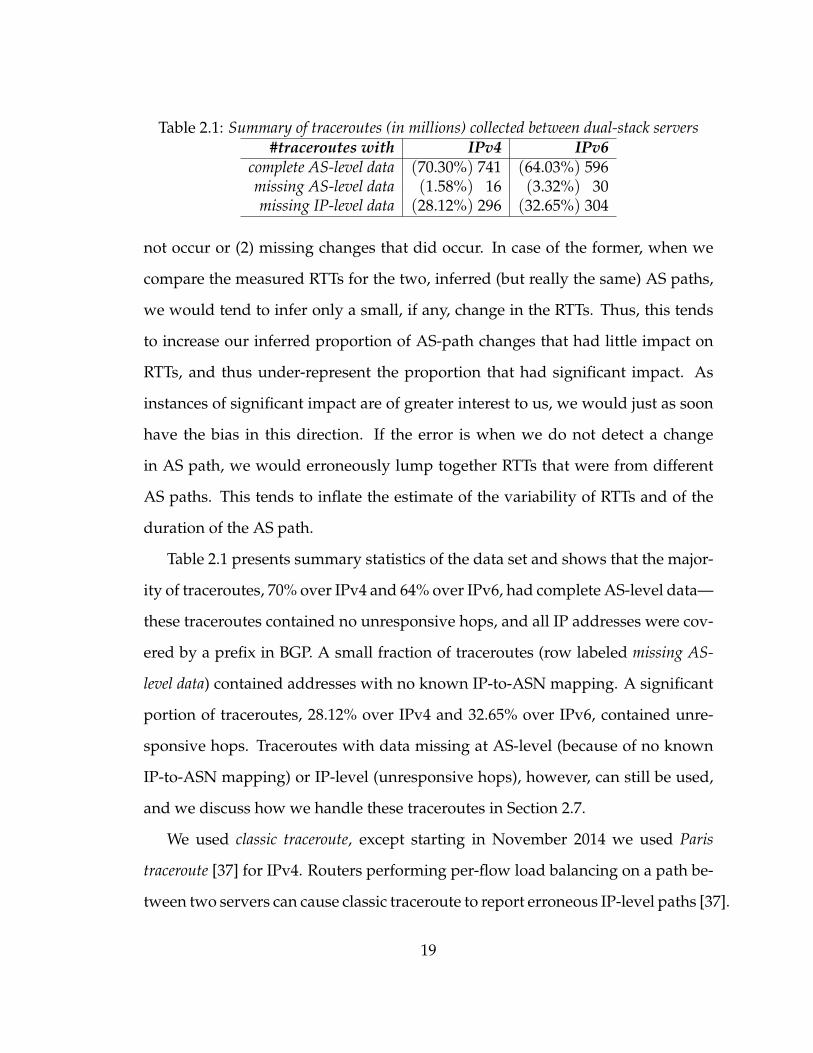
Table 2.1: Summary of traceroutes (in millions) collected between dual-stack servers#traceroutes with IPv4 IPv6

complete AS-level data (70.30%) 741 (64.03%) 596missing AS-level data (1.58%) 16 (3.32%) 30missing IP-level data (28.12%) 296 (32.65%) 304

not occur or (2) missing changes that did occur. In case of the former, when we

compare the measured RTTs for the two, inferred (but really the same) AS paths,

we would tend to infer only a small, if any, change in the RTTs. Thus, this tends

to increase our inferred proportion of AS-path changes that had little impact on

RTTs, and thus under-represent the proportion that had significant impact. As

instances of significant impact are of greater interest to us, we would just as soon

have the bias in this direction. If the error is when we do not detect a change

in AS path, we would erroneously lump together RTTs that were from different

AS paths. This tends to inflate the estimate of the variability of RTTs and of the

duration of the AS path.

Table 2.1 presents summary statistics of the data set and shows that the major-

ity of traceroutes, 70% over IPv4 and 64% over IPv6, had complete AS-level data—

these traceroutes contained no unresponsive hops, and all IP addresses were cov-

ered by a prefix in BGP. A small fraction of traceroutes (row labeled missing AS-

level data) contained addresses with no known IP-to-ASN mapping. A significant

portion of traceroutes, 28.12% over IPv4 and 32.65% over IPv6, contained unre-

sponsive hops. Traceroutes with data missing at AS-level (because of no known

IP-to-ASN mapping) or IP-level (unresponsive hops), however, can still be used,

and we discuss how we handle these traceroutes in Section 2.7.

We used classic traceroute, except starting in November 2014 we used Paris

traceroute [37] for IPv4. Routers performing per-flow load balancing on a path be-

tween two servers can cause classic traceroute to report erroneous IP-level paths [37].

19

The AS path inferred from classic traceroute data can contain loops in AS paths,

though it is rare for the classic traceroute algorithm to be the cause [137]. A small

fraction of traceroutes, 2.16% over IPv4 and 5.5% over IPv6, contain AS-path loops

and were not included in the analyses. Because our measurement platform is a

production CDN, we can neither run experiments with modified versions of sup-

ported protocols (or tools), nor add support for other protocols (or install new

tools), viz., Tokyo Ping [171].

The AS paths inferred from the traceroutes gathered during the 16-month study

period cover 722 unique networks (ASes) over IPv4 and 578 over IPv6. While

there exist no authoritative list of Tier 1 networks, we find that all well-known

Tier 1 networks [215] are captured in our traceroutes. Indeed, ranking the net-

works by the number of traceroutes in which they appear reveals that the top 10

networks, with the exception of Akamai Technologies and Integra Telecom, are

Tier 1 network providers.

2.4.3 Short-term Measurements

We performed a series of measurements over smaller time scales (one or more

weeks) to measure short-term trends in performance characteristics of server-to-

server paths. We analyzed server-to-server ping data collected by the CDN from

February 22nd through 28th, 2015. Servers from each one of the several thousand

clusters around the world ping a predetermined set of servers in other clusters

every 15 minutes to gather performance statistics. The ping data set contained

more than 2.9M IPv4 and approximately 1M IPv6 server pairs, each of which

had at least 600 measurements (i.e., nearly 90% or more of the total 672 possible

measurements per server pair).

Using the ping measurements, we identified 100K server pairs where we ob-

served diurnal patterns in the end-to-end RTTs, indicative of congestion (see Sec-

20

tion 2.8). We chose a subset of 50K server pairs to ensure that the traceroute mea-

surements between the selected pairs complete in under 30 minutes. The selec-

tion consists of servers from around 3.5K server clusters, located in more than

1000 locations and 100 countries. We repeated the traceroutes, over both IPv4 and

IPv6, between the selected server pairs, in either direction, once every 30 minutes

for more than two consecutive weeks. Finally, to infer congestion between clus-

ters at the same location we performed traceroute campaigns between all servers

(full mesh) colocated at the same datacenter or peering facility with a frequency

of 30 minutes for a period of 20 days. During the measurement campaigns, we

monitored and analyzed the logs of the servers to ensure that servers were not

experiencing high loads and to handle operational disruptions such as routing

maintenance.

2.5 Back-Office Traffic

A CDN can be viewed as a high-bandwidth low-latency conduit that facilitates

data exchanges between end users and different points of origin. They are one of

the major contributors to back-office traffic. In this section, we highlight the in-

sights offered by CDN server logs into server-to-server or back-office Web traffic.

2.5.1 Front-office vs. back-office CDN traffic

The primary focus of a CDN is to serve content to the user as efficiently as possi-

ble. Therefore, one should expect CDN front-office traffic to dominate CDN back-

office traffic in volume. As not all content is cacheable [24], up to date, or popular,

some content has to be fetched from other servers. Moreover, many CDNs, e.g.,

Akamai [198], create and maintain sophisticated overlays to interconnect their

edge servers and origin servers to improve end-to-end performance, to by-pass

network bottlenecks, and to increase tolerance to network or path failures. Hence,

21

a CDN edge server may contact, besides origin servers, other CDN servers located

either in the same cluster, with back-office Web traffic routed over a private net-

work, or in a different cluster at the same or different location, with the back-office

Web traffic routed over a private or public network.

With the knowledge of the IP addresses used by the CDN’s infrastructure, we

differentiate the intra-CDN Web traffic from the traffic between the CDN servers

and end users (CDN-EndUsers), and CDN servers and origin servers (CDN-Origin).

Furthermore, within the class of intra-CDN Web traffic, we differentiate the traffic

between servers in the same cluster from that between servers in different clus-

ters; traffic between servers in the same cluster uses high-capacity low-latency

links and is routed over a private network (Intra-CDN/Private). We note that

this traffic does not qualify as back-office Web traffic routed over the public Inter-

net, which is the main focus of this section. But in order to properly account for

the publicly-routed back-office traffic that we are interested in, we must be able

to separate out the Intra-CDN/Private traffic. Note also that since this category

of back-office Web traffic is not routed via the public Internet it does not accrue

any peering cost or hosting cost. Our classification scheme partitions the Web

traffic identified via the logs into four categories: (1) CDN-EndUsers, (2) Intra-

CDN/Public, (3) Intra-CDN/Private, and (4) CDN-Origin.

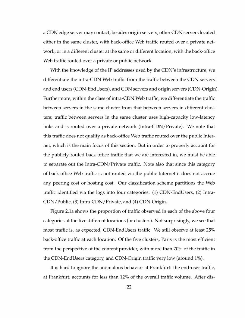
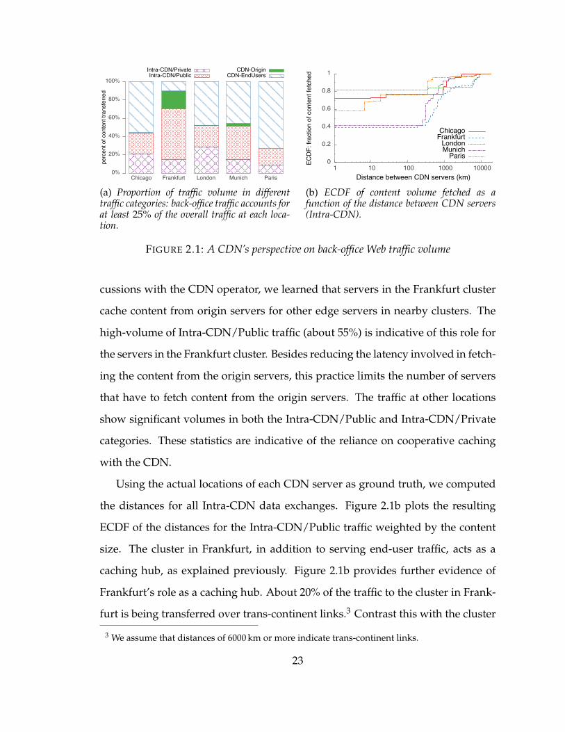
Figure 2.1a shows the proportion of traffic observed in each of the above four

categories at the five different locations (or clusters). Not surprisingly, we see that

most traffic is, as expected, CDN-EndUsers traffic. We still observe at least 25%

back-office traffic at each location. Of the five clusters, Paris is the most efficient

from the perspective of the content provider, with more than 70% of the traffic in

the CDN-EndUsers category, and CDN-Origin traffic very low (around 1%).

It is hard to ignore the anomalous behavior at Frankfurt: the end-user traffic,

at Frankfurt, accounts for less than 12% of the overall traffic volume. After dis-

22

��

��

��

��

��

��

��

��

��

��

(a) Proportion of traffic volume in differenttraffic categories: back-office traffic accounts forat least 25% of the overall traffic at each loca-tion.

��

��

��

��

��

��

��

��

��

��

(b) ECDF of content volume fetched as afunction of the distance between CDN servers(Intra-CDN).

FIGURE 2.1: A CDN’s perspective on back-office Web traffic volume

cussions with the CDN operator, we learned that servers in the Frankfurt cluster

cache content from origin servers for other edge servers in nearby clusters. The

high-volume of Intra-CDN/Public traffic (about 55%) is indicative of this role for

the servers in the Frankfurt cluster. Besides reducing the latency involved in fetch-

ing the content from the origin servers, this practice limits the number of servers

that have to fetch content from the origin servers. The traffic at other locations

show significant volumes in both the Intra-CDN/Public and Intra-CDN/Private

categories. These statistics are indicative of the reliance on cooperative caching

with the CDN.

Using the actual locations of each CDN server as ground truth, we computed

the distances for all Intra-CDN data exchanges. Figure 2.1b plots the resulting

ECDF of the distances for the Intra-CDN/Public traffic weighted by the content

size. The cluster in Frankfurt, in addition to serving end-user traffic, acts as a

caching hub, as explained previously. Figure 2.1b provides further evidence of

Frankfurt’s role as a caching hub. About 20% of the traffic to the cluster in Frank-

furt is being transferred over trans-continent links.3 Contrast this with the cluster

3 We assume that distances of 6000 km or more indicate trans-continent links.

23

��

��

��

��

��

��

��

��

��

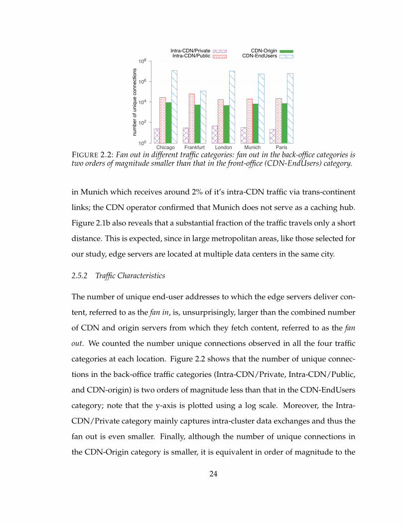
FIGURE 2.2: Fan out in different traffic categories: fan out in the back-office categories istwo orders of magnitude smaller than that in the front-office (CDN-EndUsers) category.

in Munich which receives around 2% of it’s intra-CDN traffic via trans-continent

links; the CDN operator confirmed that Munich does not serve as a caching hub.

Figure 2.1b also reveals that a substantial fraction of the traffic travels only a short

distance. This is expected, since in large metropolitan areas, like those selected for

our study, edge servers are located at multiple data centers in the same city.

2.5.2 Traffic Characteristics

The number of unique end-user addresses to which the edge servers deliver con-

tent, referred to as the fan in, is, unsurprisingly, larger than the combined number

of CDN and origin servers from which they fetch content, referred to as the fan

out. We counted the number unique connections observed in all the four traffic

categories at each location. Figure 2.2 shows that the number of unique connec-

tions in the back-office traffic categories (Intra-CDN/Private, Intra-CDN/Public,

and CDN-origin) is two orders of magnitude less than that in the CDN-EndUsers

category; note that the y-axis is plotted using a log scale. Moreover, the Intra-

CDN/Private category mainly captures intra-cluster data exchanges and thus the

fan out is even smaller. Finally, although the number of unique connections in

the CDN-Origin category is smaller, it is equivalent in order of magnitude to the

24

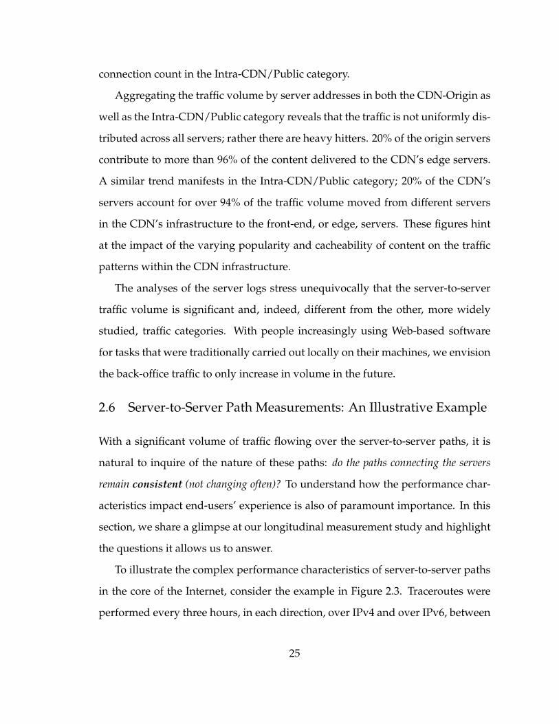
connection count in the Intra-CDN/Public category.

Aggregating the traffic volume by server addresses in both the CDN-Origin as

well as the Intra-CDN/Public category reveals that the traffic is not uniformly dis-

tributed across all servers; rather there are heavy hitters. 20% of the origin servers

contribute to more than 96% of the content delivered to the CDN’s edge servers.

A similar trend manifests in the Intra-CDN/Public category; 20% of the CDN’s

servers account for over 94% of the traffic volume moved from different servers

in the CDN’s infrastructure to the front-end, or edge, servers. These figures hint

at the impact of the varying popularity and cacheability of content on the traffic

patterns within the CDN infrastructure.

The analyses of the server logs stress unequivocally that the server-to-server

traffic volume is significant and, indeed, different from the other, more widely

studied, traffic categories. With people increasingly using Web-based software

for tasks that were traditionally carried out locally on their machines, we envision

the back-office traffic to only increase in volume in the future.

2.6 Server-to-Server Path Measurements: An Illustrative Example

With a significant volume of traffic flowing over the server-to-server paths, it is

natural to inquire of the nature of these paths: do the paths connecting the servers

remain consistent (not changing often)? To understand how the performance char-

acteristics impact end-users’ experience is also of paramount importance. In this

section, we share a glimpse at our longitudinal measurement study and highlight

the questions it allows us to answer.

To illustrate the complex performance characteristics of server-to-server paths

in the core of the Internet, consider the example in Figure 2.3. Traceroutes were

performed every three hours, in each direction, over IPv4 and over IPv6, between

25

0

50

100

150

200

250

300

350

400

Jan Feb Mar AprApr May Jun Jul

RTT (in

ms)

IPv4IPv6

FIGURE 2.3: A six-month timeline of RTTs observed in traceroutes from a server in HongKong, HK to a server in Osaka, JP exhibiting level shifts (compare RTTs in March withthat in June).

dual-stack servers, one located in a datacenter in Hong Kong and the other in

Osaka, Japan. The figure shows the RTTs between the endpoints (from Hong Kong

to Japan) for the first six months of 2014. Focusing first on the RTTs over IPv4 (the

red line), an obvious feature is level shifts between periods of a baseline RTT with

variability above the baseline. During periods where the baseline RTT was above

150 ms the traceroute went via the west coast of the USA. We inferred the AS paths

from the traceroutes, and at each of the level shifts there was a change in the AS

path in one, or both, directions. Also, there were cases where the AS path changed,

but there was a negligible change in the RTTs. This leads to the first theme of this

chapter: to what extent do changes in the AS path affect round-trip times?

Another key feature of the plot is the spikes in RTT, which are a typical fea-

ture of repeated measurements. Figure 2.4 shows the daily oscillation in RTT (as

opposed to individual spikes) during the period between March 26 and April 2,

2014; this also occurs from February 14th to 22nd. A daily oscillation in RTT is often

an indication of congestion during the busy period of the day somewhere along

26

50

100

150

200

250

300

350

03/26 03/27 03/28 03/29 03/30 03/31 04/01 04/02

RTT (in

ms)

IPv4IPv6

Night Day

FIGURE 2.4: A small section of the RTTs’ timeline exhibiting daily variations (observethe repeating mid-day increases).

the path, or at an endpoint4. A second theme of this chapter is: how common are

periods of daily oscillation in RTT, and where do they occur?

One can ask the higher level question: what affects end-to-end performance more—

routing or congestion? In Figure 2.3, changes in routing seemed to have a greater

impact on RTT.

Now consider the RTTs measured over IPv6 (the blue line). To first order, it

has similar features as IPv4 (the red line). A notable level shift is on April 21,

2014, where the route for IPv6 got much better at the same time that it got worse

for IPv4; RTTs increased by 108 ms over IPv4, and decreased by 168 ms over IPv6.

During March 26th to April 2nd, the path over IPv6 also experienced a daily oscil-

lation in RTTs, which could have been occurring at equipment that was in both

the IPv4 and IPv6 path. A third theme of this chapter is: how does IPv4 and IPv6

4 The probes were ICMP, and routers may handle them differently from UDP and TCP. Thus,traffic to/from end users may not experience the same degradation as the ICMP probes. Nev-ertheless, that the ICMP packets did experience the daily oscillation in RTT is evidence of somestress on some equipment on the path, and could foreshadow degradation in performance for theuser traffic.

27

compare with respect to routing and performance?

We would like to stress that the example we selected for illustration serves

only as a candidate to highlight interesting observations, the challenges inherent

in observing and quantifying them, and interesting research questions that arise.

While it is trivial to analyze manually a few cherry-picked examples, it becomes

impractical after considering only a few tens of server pairs.

2.7 Impact of Routing Changes

We investigated, using the long-term data set, the impact of routing changes in

the core on end-to-end RTTs between server pairs. For simplicity, we restricted

our attention to a set of 60K server-pairs that, for at least 400 days (of the 485 days

of data collection) had, on each day, at least one traceroute between them in both

directions and over both IPv4 and IPv6 protocols. We conclude this section with

a brief analysis using the short-term data set showing that the coarse granularity

of measurements in the long-term data set likely does not affect our results.

2.7.1 Methodology for Inferring Changes

To capture routing changes along the path between any two servers, we treat the

AS paths (with each hop representing a different ASN) between the servers as

delimited strings and use the edit distance between any two AS paths as a measure

of the difference between them. A zero edit distance implies that the AS paths are

the same (no change), while a non-zero value implies a different AS-level route.

Suppose AS paths p1 : ASNa Ñ ASNb Ñ ASNc Ñ ASNd and p2 : ASNa Ñ

ASNb Ñ ASNd were observed in traceroutes between two servers A and B at time

t1 and t2, respectively. The edit distance computation on the path-strings yields

the value one, implying that the paths are different and one change (removal of

ASNc) is required to make p1 identical to p2. We also assume that the routing

28

change from p1 to p2 happened at t2. Traceroutes may contain one or more hops

either with no IP address (i. e., non-responsive hop) or with an IP address having

no known IP-to-ASN mapping. Although, we cannot eliminate all missing data,

we impute the missing hop (at only the AS-level) in instances where either side of

the missing hop is the same ASN.

Computing Lifetimes. Since our data set contains only one traceroute between

any two servers during each three-hour time period, we assumed an AS path ob-

served from a traceroute to persist for three hours. For instance, AS path p1, in the

example above, is assumed to persist during the time interval [t1, t2), assuming

t1 and t2 are consecutive three-hour time intervals (i. e., t1 + 3 hours = t2). The

lifetime of an AS path with respect to a set of endpoints is defined as the total time

during which the AS path was observed between the endpoints. For instance, if

path p1 was observed 800 times (the periods during which p1 was observed do

not need be contiguous) in traceroutes from server A to B, the lifetime of p1 is

calculated as 2400 hours (100 days). The AS-path in the other direction (from B to

A) might have a different lifetime depending on how many times, if any, the path

was observed. We also refer to the set of all traceroutes from one server to an-

other (representing a time series) as a trace timeline. As an example, all traceroutes

with source as server A and destination as server B over the period of 16-months

constitute one trace timeline.

In the subsequent sections, we characterize the AS-paths we observe between

the servers and analyze the frequency of changes in AS-path in different trace

timelines. We show how these changes in AS-paths affect the end-to-end latency

of the server-to-server paths.

29

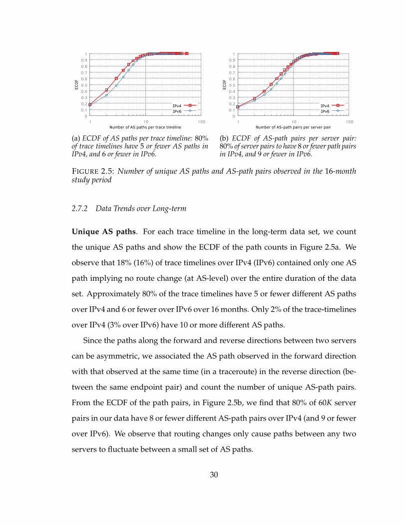
0 0.1 0.2 0.3 0.4 0.5 0.6 0.7 0.8 0.9

1

1 10 100

ECDF

Number of AS paths per trace timeline

IPv4IPv6

(a) ECDF of AS paths per trace timeline: 80%of trace timelines have 5 or fewer AS paths inIPv4, and 6 or fewer in IPv6.

0 0.1 0.2 0.3 0.4 0.5 0.6 0.7 0.8 0.9

1

1 10 100

ECDF

Number of AS-path pairs per server pair

IPv4IPv6

(b) ECDF of AS-path pairs per server pair:80% of server pairs to have 8 or fewer path pairsin IPv4, and 9 or fewer in IPv6.

FIGURE 2.5: Number of unique AS paths and AS-path pairs observed in the 16-monthstudy period

2.7.2 Data Trends over Long-term

Unique AS paths. For each trace timeline in the long-term data set, we count

the unique AS paths and show the ECDF of the path counts in Figure 2.5a. We

observe that 18% (16%) of trace timelines over IPv4 (IPv6) contained only one AS

path implying no route change (at AS-level) over the entire duration of the data

set. Approximately 80% of the trace timelines have 5 or fewer different AS paths

over IPv4 and 6 or fewer over IPv6 over 16 months. Only 2% of the trace-timelines

over IPv4 (3% over IPv6) have 10 or more different AS paths.

Since the paths along the forward and reverse directions between two servers

can be asymmetric, we associated the AS path observed in the forward direction

with that observed at the same time (in a traceroute) in the reverse direction (be-

tween the same endpoint pair) and count the number of unique AS-path pairs.

From the ECDF of the path pairs, in Figure 2.5b, we find that 80% of 60K server

pairs in our data have 8 or fewer different AS-path pairs over IPv4 (and 9 or fewer

over IPv6). We observe that routing changes only cause paths between any two

servers to fluctuate between a small set of AS paths.

30

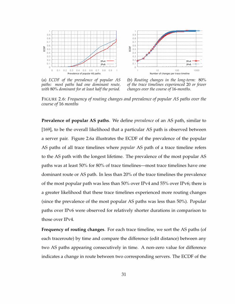
0 0.1 0.2 0.3 0.4 0.5 0.6 0.7 0.8 0.9

1

0 0.1 0.2 0.3 0.4 0.5 0.6 0.7 0.8 0.9 1

ECDF

Prevalence of popular AS paths

IPv4IPv6

(a) ECDF of the prevalence of popular ASpaths: most paths had one dominant route,with 80% dominant for at least half the period.

0 0.1 0.2 0.3 0.4 0.5 0.6 0.7 0.8 0.9

1

1 10 100 1000

ECDF

Number of changes per trace timeline

IPv4IPv6

(b) Routing changes in the long-term: 80%of the trace timelines experienced 20 or fewerchanges over the course of 16-months.

FIGURE 2.6: Frequency of routing changes and prevalence of popular AS paths over thecourse of 16 months

Prevalence of popular AS paths. We define prevalence of an AS path, similar to

[169], to be the overall likelihood that a particular AS path is observed between

a server pair. Figure 2.6a illustrates the ECDF of the prevalence of the popular

AS paths of all trace timelines where popular AS path of a trace timeline refers

to the AS path with the longest lifetime. The prevalence of the most popular AS

paths was at least 50% for 80% of trace timelines—most trace timelines have one

dominant route or AS path. In less than 20% of the trace timelines the prevalence

of the most popular path was less than 50% over IPv4 and 55% over IPv6; there is

a greater likelihood that these trace timelines experienced more routing changes

(since the prevalence of the most popular AS paths was less than 50%). Popular

paths over IPv6 were observed for relatively shorter durations in comparison to

those over IPv4.

Frequency of routing changes. For each trace timeline, we sort the AS paths (of

each traceroute) by time and compare the difference (edit distance) between any

two AS paths appearing consecutively in time. A non-zero value for difference

indicates a change in route between two corresponding servers. The ECDF of the

31

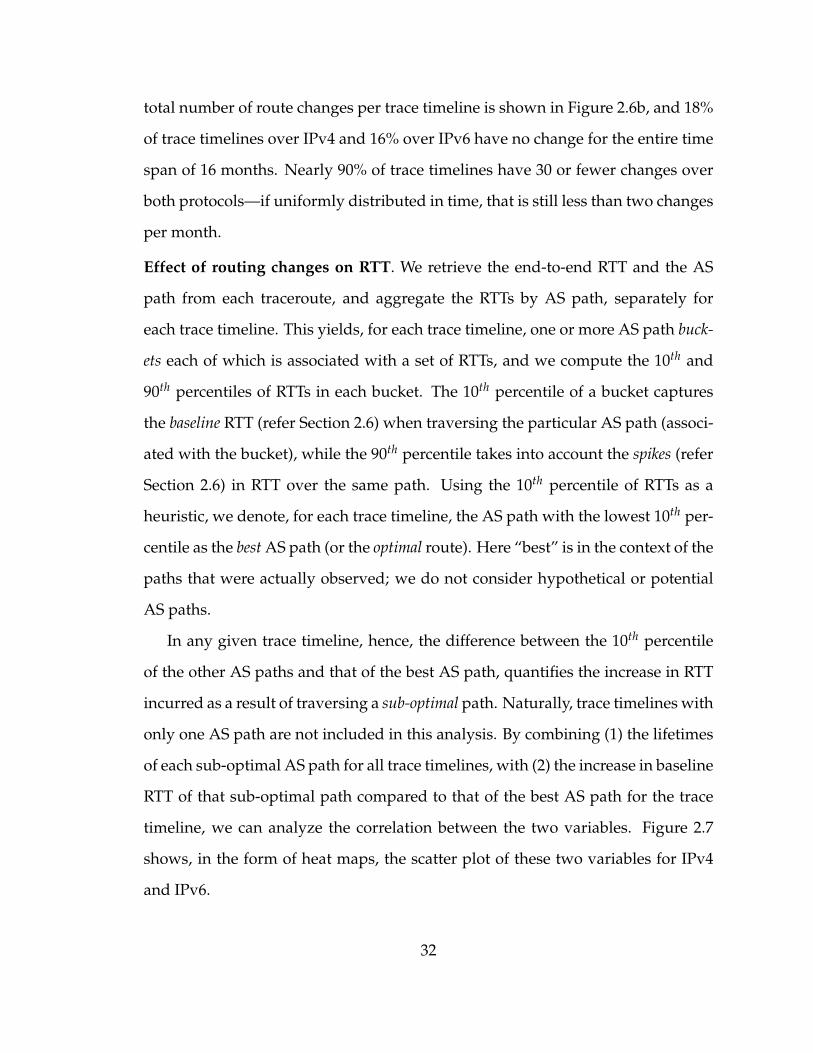
total number of route changes per trace timeline is shown in Figure 2.6b, and 18%

of trace timelines over IPv4 and 16% over IPv6 have no change for the entire time

span of 16 months. Nearly 90% of trace timelines have 30 or fewer changes over

both protocols—if uniformly distributed in time, that is still less than two changes

per month.

Effect of routing changes on RTT. We retrieve the end-to-end RTT and the AS

path from each traceroute, and aggregate the RTTs by AS path, separately for

each trace timeline. This yields, for each trace timeline, one or more AS path buck-

ets each of which is associated with a set of RTTs, and we compute the 10th and

90th percentiles of RTTs in each bucket. The 10th percentile of a bucket captures

the baseline RTT (refer Section 2.6) when traversing the particular AS path (associ-

ated with the bucket), while the 90th percentile takes into account the spikes (refer

Section 2.6) in RTT over the same path. Using the 10th percentile of RTTs as a

heuristic, we denote, for each trace timeline, the AS path with the lowest 10th per-

centile as the best AS path (or the optimal route). Here “best” is in the context of the

paths that were actually observed; we do not consider hypothetical or potential

AS paths.

In any given trace timeline, hence, the difference between the 10th percentile

of the other AS paths and that of the best AS path, quantifies the increase in RTT

incurred as a result of traversing a sub-optimal path. Naturally, trace timelines with

only one AS path are not included in this analysis. By combining (1) the lifetimes

of each sub-optimal AS path for all trace timelines, with (2) the increase in baseline

RTT of that sub-optimal path compared to that of the best AS path for the trace

timeline, we can analyze the correlation between the two variables. Figure 2.7

shows, in the form of heat maps, the scatter plot of these two variables for IPv4

and IPv6.

32

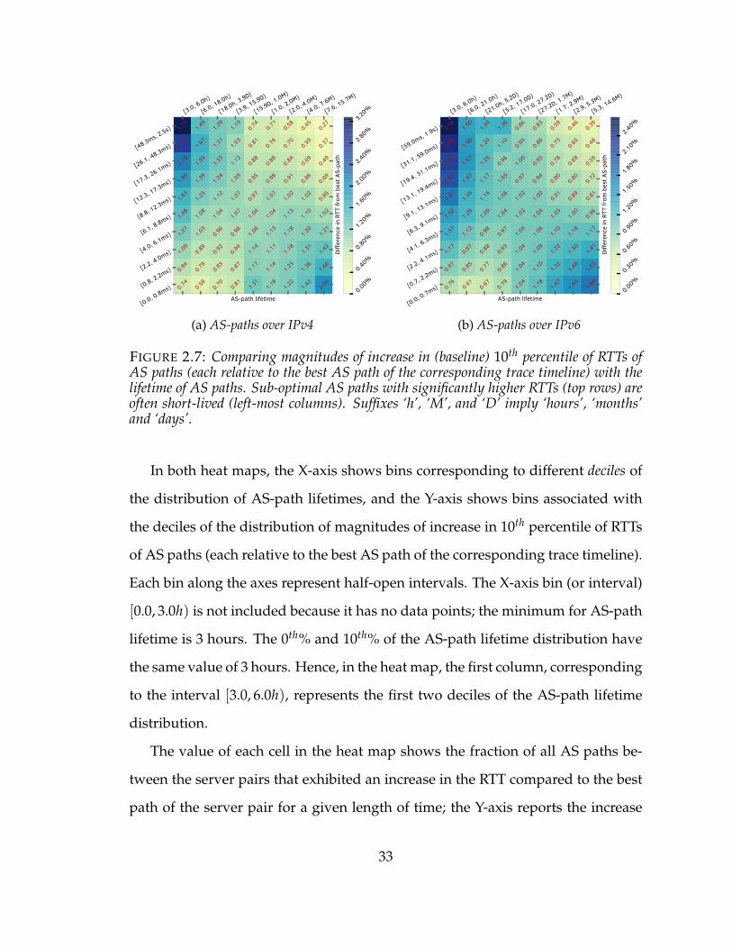
[3.0, 6.0h)

[6.0, 18.0h)

[18.0h, 3.9D)

[3.9, 15.9D)

[15.9D, 1.0M)

[1.0, 2.0M)

[2.0, 4.0M)

[4.0, 7.6M)

[7.6, 15.7M)

AS-path lifetime[0.0, 0.8ms)[0.8, 2.2ms)[2.2, 4.0ms)[4.0, 6.1ms)[6.1, 8.8ms)[8.8, 12.3ms)[12.3, 17.3ms)[17.3, 26.1ms)[26.1, 48.3ms)[48.3ms, 2.5s)

Diffe

renc

e in

RTT

from

bes

t AS-

path

0.74

0.94

1.09

1.27

1.48

1.63

1.89

2.18

2.77

3.29

0.58

0.79

0.89

1.03

1.08

1.25

1.39

1.59

1.67

1.49

0.70

0.83

0.92

0.96

1.04

1.12

1.24

1.33

1.31

1.29

0.81

0.87

0.94

0.98

1.07

1.07

1.09

1.12

1.03

1.19

1.31

1.17

1.14

1.06

1.04

0.97

0.95

0.88

0.81

0.74

1.18

1.14

1.11

1.13

1.04

1.07

0.98

0.88

0.76

0.71

1.22

1.23

1.18

1.18

1.13

1.02

0.91

0.84

0.70

0.58

1.42

1.36

1.31

1.20

1.10

1.02

0.86

0.69

0.59

0.45

2.04

1.66

1.42

1.21

1.02

0.85

0.69

0.49

0.37

0.27

0.00%

0.40%

0.80%

1.20%

1.60%

2.00%

2.40%

2.80%

3.20%

(a) AS-paths over IPv4

[3.0, 6.0h)

[6.0, 21.0h)

[21.0h, 5.2D)

[5.2, 17.0D)

[17.0, 27.2D)

[27.2D, 1.7M)

[1.7, 2.9M)

[2.9, 5.3M)

[5.3, 14.6M)


Diffe

renc

e in

RTT

from

bes

t AS-

path

0.76

0.97

1.17

1.37

1.52

1.81

2.07

2.22

2.46

2.68

0.61

0.85

0.97

1.12

1.29

1.35

1.47

1.57

1.56

1.50

0.67

0.77

0.88

0.98

1.09

1.16

1.17

1.25

1.20

1.34

0.79

0.86

0.93

0.97

1.04

1.06

1.05

0.96

1.10

1.36

1.04

1.04

1.04

1.05

1.02

1.02

0.97

1.00

0.95

0.86

1.18

1.10

1.09

1.06

1.04

1.00

0.94

0.93

0.88

0.83

1.47

1.32

1.22

1.10

1.03

0.91

0.80

0.78

0.73

0.59

1.64

1.46

1.30

1.16

1.00

0.89

0.80

0.69

0.65

0.46

1.84

1.63

1.41

1.17

0.96

0.81

0.72

0.59

0.48

0.39

0.00%

0.30%

0.60%

0.90%

1.20%

1.50%

1.80%

2.10%

2.40%

(b) AS-paths over IPv6

FIGURE 2.7: Comparing magnitudes of increase in (baseline) 10th percentile of RTTs ofAS paths (each relative to the best AS path of the corresponding trace timeline) with thelifetime of AS paths. Sub-optimal AS paths with significantly higher RTTs (top rows) areoften short-lived (left-most columns). Suffixes ‘h’, ‘M’, and ‘D’ imply ‘hours’, ‘months’and ‘days’.

In both heat maps, the X-axis shows bins corresponding to different deciles of

the distribution of AS-path lifetimes, and the Y-axis shows bins associated with

the deciles of the distribution of magnitudes of increase in 10th percentile of RTTs

of AS paths (each relative to the best AS path of the corresponding trace timeline).

Each bin along the axes represent half-open intervals. The X-axis bin (or interval)

[0.0, 3.0h) is not included because it has no data points; the minimum for AS-path

lifetime is 3 hours. The 0th% and 10th% of the AS-path lifetime distribution have

the same value of 3 hours. Hence, in the heat map, the first column, corresponding

to the interval [3.0, 6.0h), represents the first two deciles of the AS-path lifetime

distribution.

The value of each cell in the heat map shows the fraction of all AS paths be-

tween the server pairs that exhibited an increase in the RTT compared to the best

path of the server pair for a given length of time; the Y-axis reports the increase

33

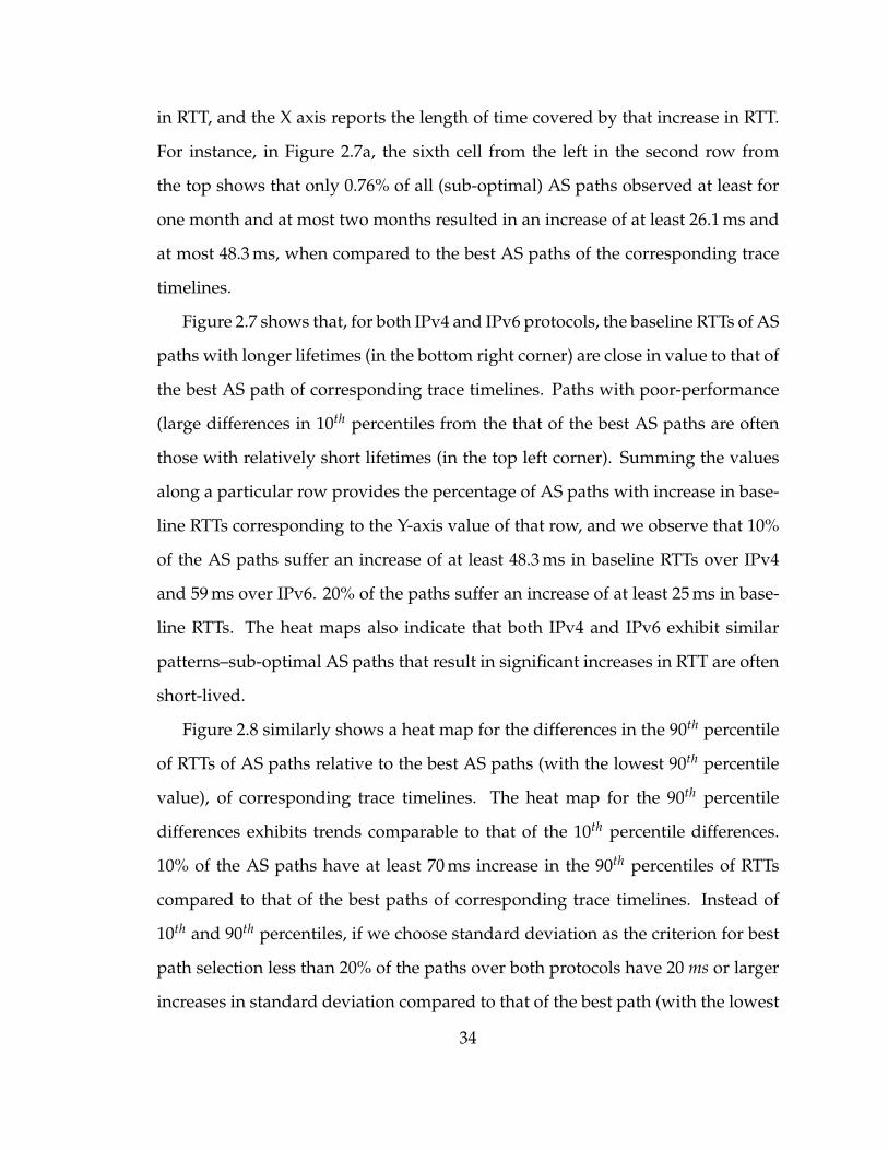
in RTT, and the X axis reports the length of time covered by that increase in RTT.

For instance, in Figure 2.7a, the sixth cell from the left in the second row from

the top shows that only 0.76% of all (sub-optimal) AS paths observed at least for

one month and at most two months resulted in an increase of at least 26.1 ms and

at most 48.3 ms, when compared to the best AS paths of the corresponding trace

timelines.

Figure 2.7 shows that, for both IPv4 and IPv6 protocols, the baseline RTTs of AS

paths with longer lifetimes (in the bottom right corner) are close in value to that of

the best AS path of corresponding trace timelines. Paths with poor-performance

(large differences in 10th percentiles from the that of the best AS paths are often

those with relatively short lifetimes (in the top left corner). Summing the values

along a particular row provides the percentage of AS paths with increase in base-

line RTTs corresponding to the Y-axis value of that row, and we observe that 10%

of the AS paths suffer an increase of at least 48.3 ms in baseline RTTs over IPv4

and 59 ms over IPv6. 20% of the paths suffer an increase of at least 25 ms in base-

line RTTs. The heat maps also indicate that both IPv4 and IPv6 exhibit similar

patterns–sub-optimal AS paths that result in significant increases in RTT are often

short-lived.

Figure 2.8 similarly shows a heat map for the differences in the 90th percentile

of RTTs of AS paths relative to the best AS paths (with the lowest 90th percentile

value), of corresponding trace timelines. The heat map for the 90th percentile

differences exhibits trends comparable to that of the 10th percentile differences.

10% of the AS paths have at least 70 ms increase in the 90th percentiles of RTTs

compared to that of the best paths of corresponding trace timelines. Instead of

10th and 90th percentiles, if we choose standard deviation as the criterion for best

path selection less than 20% of the paths over both protocols have 20 ms or larger

increases in standard deviation compared to that of the best path (with the lowest

34

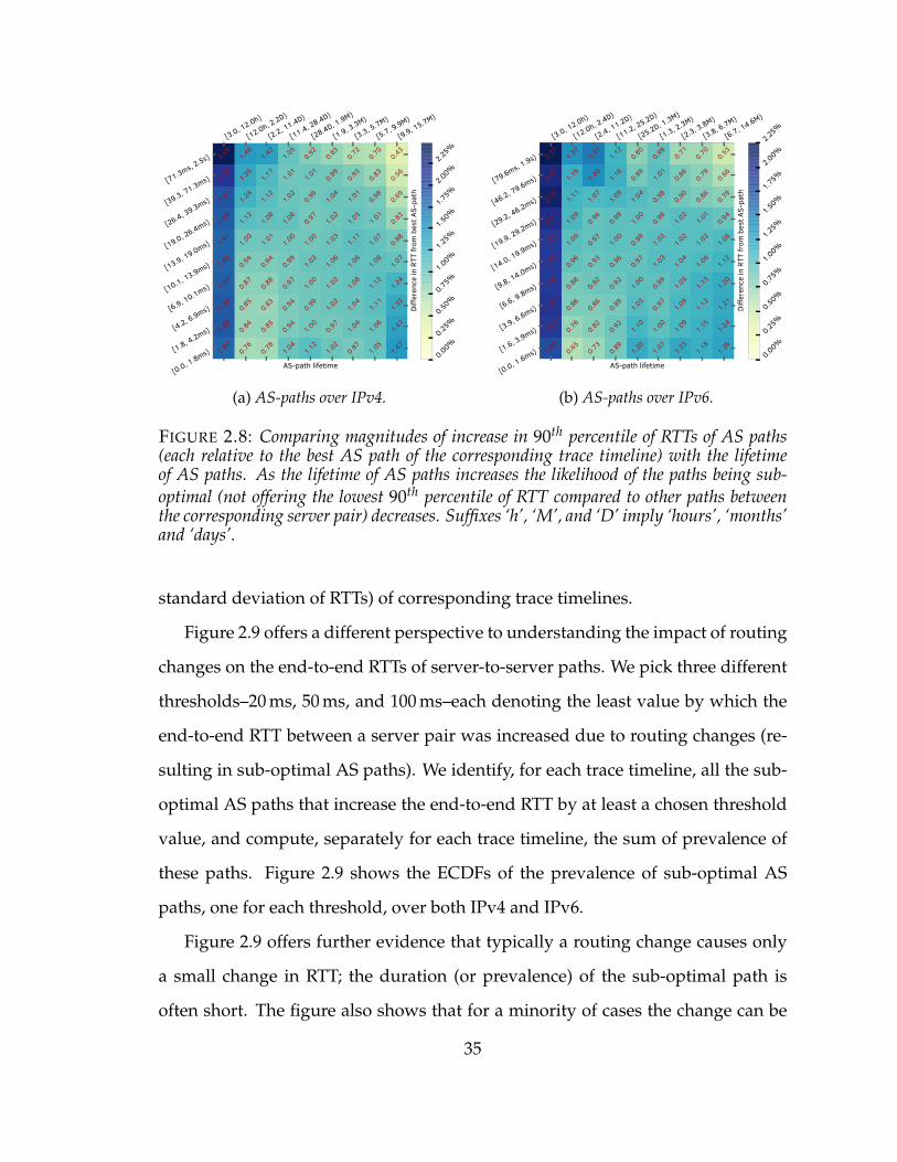
[3.0, 12.0h)

[12.0h, 2.2D)

[2.2, 11.4D)

[11.4, 28.4D)

[28.4D, 1.9M)

[1.9, 3.3M)

[3.3, 5.7M)

[5.7, 9.9M)

[9.9, 15.7M)


Diffe

renc

e in

RTT

from

bes

t AS-

path

1.80

1.89

1.88

1.84

1.82

1.81

1.86

1.91

2.16

2.48

0.76

0.84

0.85

0.87

0.94

1.00

1.12

1.24

1.35

1.46

0.78

0.85

0.83

0.88

0.94

1.01

1.08

1.12

1.17

1.42

1.04

0.94

0.94

0.97

0.99

1.00

1.06

1.02

1.01

1.05

1.12

1.00

0.99

1.00

1.03

1.00

0.97

0.99

1.01

0.92

1.02

0.97

1.02

1.02

1.06

1.03

1.02

1.04

0.99

0.83

0.97

1.04

1.04

1.08

1.08

1.11

1.05

1.01

0.93

0.72

1.05

1.06

1.11

1.12

1.08

1.07

1.01

0.98

0.83

0.70

1.47

1.41

1.33

1.24

1.07

0.98

0.83

0.69

0.56

0.43

0.00%0.25%0.50%0.75%1.00%1.25%1.50%1.75%2.00%2.25%

(a) AS-paths over IPv4.

[3.0, 12.0h)

[12.0h, 2.4D)

[2.4, 11.2D)

[11.2, 25.2D)

[25.2D, 1.3M)

[1.3, 2.3M)

[2.3, 3.8M)

[3.8, 6.7M)

[6.7, 14.6M)


Diffe

renc

e in

RTT

from

bes

t AS-

path

1.80

1.93

1.97

1.92

1.93

1.93

2.01

2.16

2.07

2.25

0.65

0.76

0.86

0.88

0.96

1.00

1.09

1.11

1.16

1.37

0.73

0.82

0.86

0.92

0.93

0.97

0.96

1.07

1.40

1.51

0.89

0.92

0.89

0.92

0.96

1.00

0.99

1.09

1.16

1.12

1.20

1.10

1.03

1.00

0.97

0.99

1.00

1.04

0.89

0.80

1.07

1.00

0.97

0.99

1.03

1.02

0.98

0.98

1.01

0.98

1.23

1.09

1.09

1.05

1.04

1.02

1.02

0.90

0.86

0.71

1.18

1.15

1.12

1.13

1.06

1.02

1.01

0.86

0.79

0.70

1.26

1.24

1.21

1.20

1.12

1.06

0.94

0.79

0.66

0.53

0.00%

0.25%

0.50%

0.75%

1.00%

1.25%

1.50%

1.75%

2.00%

2.25%

(b) AS-paths over IPv6.

FIGURE 2.8: Comparing magnitudes of increase in 90th percentile of RTTs of AS paths(each relative to the best AS path of the corresponding trace timeline) with the lifetimeof AS paths. As the lifetime of AS paths increases the likelihood of the paths being sub-optimal (not offering the lowest 90th percentile of RTT compared to other paths betweenthe corresponding server pair) decreases. Suffixes ‘h’, ‘M’, and ‘D’ imply ‘hours’, ‘months’and ‘days’.

standard deviation of RTTs) of corresponding trace timelines.

Figure 2.9 offers a different perspective to understanding the impact of routing

changes on the end-to-end RTTs of server-to-server paths. We pick three different

thresholds–20 ms, 50 ms, and 100 ms–each denoting the least value by which the

end-to-end RTT between a server pair was increased due to routing changes (re-

sulting in sub-optimal AS paths). We identify, for each trace timeline, all the sub-

optimal AS paths that increase the end-to-end RTT by at least a chosen threshold

value, and compute, separately for each trace timeline, the sum of prevalence of

these paths. Figure 2.9 shows the ECDFs of the prevalence of sub-optimal AS

paths, one for each threshold, over both IPv4 and IPv6.

Figure 2.9 offers further evidence that typically a routing change causes only

a small change in RTT; the duration (or prevalence) of the sub-optimal path is

often short. The figure also shows that for a minority of cases the change can be

35

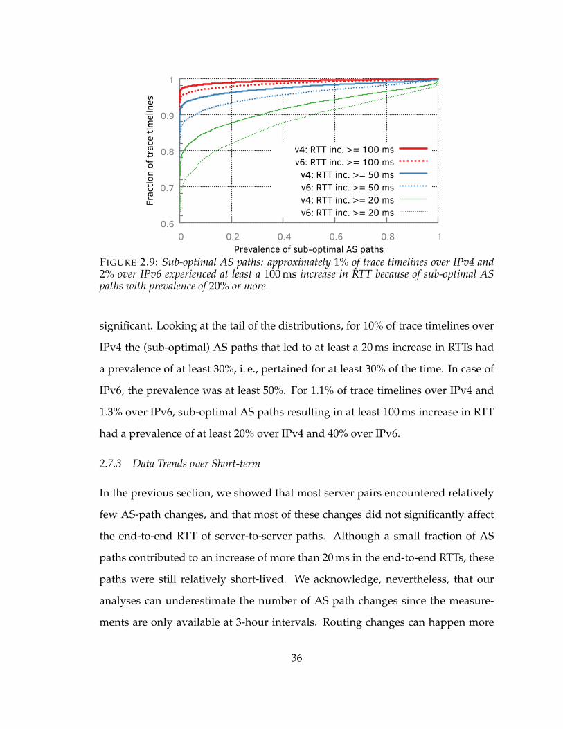
0.6

0.7

0.8

0.9

1

0 0.2 0.4 0.6 0.8 1

Frac

tion of

trac

e tim

elines

Prevalence of sub-optimal AS paths

v4: RTT inc. >= 100 msv6: RTT inc. >= 100 msv4: RTT inc. >= 50 msv6: RTT inc. >= 50 msv4: RTT inc. >= 20 msv6: RTT inc. >= 20 ms

FIGURE 2.9: Sub-optimal AS paths: approximately 1% of trace timelines over IPv4 and2% over IPv6 experienced at least a 100 ms increase in RTT because of sub-optimal ASpaths with prevalence of 20% or more.

significant. Looking at the tail of the distributions, for 10% of trace timelines over

IPv4 the (sub-optimal) AS paths that led to at least a 20 ms increase in RTTs had

a prevalence of at least 30%, i. e., pertained for at least 30% of the time. In case of

IPv6, the prevalence was at least 50%. For 1.1% of trace timelines over IPv4 and

1.3% over IPv6, sub-optimal AS paths resulting in at least 100 ms increase in RTT

had a prevalence of at least 20% over IPv4 and 40% over IPv6.

2.7.3 Data Trends over Short-term

In the previous section, we showed that most server pairs encountered relatively

few AS-path changes, and that most of these changes did not significantly affect

the end-to-end RTT of server-to-server paths. Although a small fraction of AS

paths contributed to an increase of more than 20 ms in the end-to-end RTTs, these

paths were still relatively short-lived. We acknowledge, nevertheless, that our

analyses can underestimate the number of AS path changes since the measure-

ments are only available at 3-hour intervals. Routing changes can happen more

36

0 0.1 0.2 0.3 0.4 0.5 0.6 0.7 0.8 0.9

1

1 10 100 1000

ECDF

Diff. in 10th-percentile of RTTs from best path

IPv4 AllIPv4 3hrIPv6 AllIPv6 3hr

(a) 10th percentile.

0 0.1 0.2 0.3 0.4 0.5 0.6 0.7 0.8 0.9

1

1 10 100 1000

ECDF

Diff. in 90th-percentile of RTTs from best path

IPv4 AllIPv4 3hrIPv6 AllIPv6 3hr

(b) 90th percentile.

FIGURE 2.10: Comparing magnitudes of increase in the (a) 10th, and (b) 90th percentilesof RTTs of AS paths (each relative to the “best” AS path of the corresponding trace time-line) in the short-term data set. Results using traceroutes conducted 3 hours apart (lineswith suffix ‘3hr’) are not different from that using traceroutes done 30 minutes apart (lineswith suffix ‘All’).

frequently than every 3-hours, and such missed events can affect the inferences

made. To assess the possible impact of the coarse granularity of measurements on

the inferences drawn from the long-term data set, we turn to a subset of our short-

term data set where measurements are made at a comparatively finer granularity.

We used nearly 60M traceroutes gathered every 30 minutes, over a period of 22

days, from March 10, 2015 to March 31, 2015, between approximately 20K servers.

For each trace timeline, we paired the end-to-end RTTs of each traceroute with

the AS path revealed by the traceroute. As explained in Section 2.7.2, we com-

pute the deviations in the 10th and 90th percentiles of RTTs of each AS path of

all trace timelines from that of the best AS path of corresponding timelines. To

assess the possible impact of the coarse granularity of measurements, we repeat

the computation, but consider only a subset of traceroutes separated by at least

3 hours in time. Figure 2.10 shows two ECDFs of the deviations in the 10th and

90th percentiles of RTTs associated with different AS paths: (a) the dotted lines,

labeled ‘IPv4 All’ and ‘IPv6 All’, refer to the deviations computed by considering

all traceroutes, and (b) the solid lines, labeled ‘IPv4 3hr’ and ‘IPv6 3hr’, refer to the

37

deviations computed by only considering the subset of traceroutes separated by

at least 3 hours. The difference between the ‘All’ and ‘3hr’ ECDFs of each protocol

is very small, indicating that the events that happen at shorter time scales likely

did not affect the overall analysis in Section 2.7.2.

2.8 Impact of Congestion

Is congestion the norm in the Internet core? Can we quantify the impact of congestion on

the end-to-end RTTs of paths between servers?—these are the questions we examine

in this section.

2.8.1 Is Congestion the Norm in the Core?

We seek to identify consistent congestion, defined as a type of congestion that has a

diurnal cycle with each instance of congestion lasting for a few hours, and quan-

tify its impact on server-to-server communication. We utilize the Time Sequence

Latency Probes (TSLP) method and the automated trace processing technique using

Fast Fourier Transform (FFT) described in [138] as follows. We apply the FFT

(with frequency f = 1/day) on the time series of end-to-end RTTs between server

pairs (as opposed to the difference in RTTs on successive hops as done in [138]).

We consider only the pairs where the power spectral density (i. e., the power signal

distribution around the frequency f ) is significant. We divide the power at fre-

quency f by the total power, and consider server pairs where this ratio is at least

0.35 (indication of strong diurnal pattern as a significant fraction of the energy is

concentrated around the 24-hour period). The above is a simplification of the code

from [138] which also detected short-lived daily variations and marginal cases. In

the rest of the section, the word congestion refers only to consistent congestion,

5 The choice of the threshold was based on empirical evidence. We manually inspected some ofthe diurnal patterns in RTTs between server pairs captured at different thresholds, and settled on0.3 as it seemed to capture the type of consistent congestion we wanted to investigate.

38

unless otherwise mentioned.

We analyzed server-to-server ping measurements collected using the CDN for

a period of one week6, from February 22 through 28, 2015. Servers located in

one of approximately 10K clusters around the world pinged a pre-selected set of

servers in other clusters every 15 minutes. The data set contains more than 2.9M

IPv4 server pairs and more than 1M IPv6 server pairs with each pair having at

least 600 (of the 672 possible) ping measurements. We calculated the difference

between the 95th and 5th percentiles of RTTs per server pair to estimate the fraction

of server pairs that experienced variations in RTTs exceeding 10 ms. Less than

9.5% of the server pairs over IPv4 and less than 4% over IPv6 observed more than

10 ms of variation in RTTs in the one-week period. When we consider server pairs

with a strong diurnal pattern that experience such large variations in RTTs, the

percentages of server pairs over IPv4 and IPv6 drops to 2% and 0.6% respectively.

This indicates that consistent congestion is not the norm in the core of the Internet;

one explanation, perhaps, is that links in the core are very often well provisioned,

since congestion in the core may affect thousands, or even millions, of end-users.

Note, however, that peering disputes have been reported to introduce long-term

congestion in the Internet core [138] and a large population of end users.

2.8.2 Locating Congestion

Unfortunately, it is not possible to infer the congested router-level links with the

ping data. To infer the congested links we perform traceroute campaigns utilizing,

both as a vantage point as well as a target, the subset of servers for which we have

evidence that the path experienced congestion, as described in the previous sec-

tion. The traceroute campaigns took place immediately after the ping campaign

6 We acknowledge that one week is a brief duration, but we manually examined a sampling ofthe plots of RTTs to confirm the existence of diurnal patterns in each day of the week.

39

and lasted for three weeks. To ensure that a traceroute campaign completes before

the next one is scheduled, we set the frequency of campaigns to 30 minutes.

We define the path from the vantage point of a traceroute to a given hop as a

segment. Moving from the first hop towards the last hop (destination) of a tracer-

oute, each segment of the traceroute contains the previous segment in its entirety

and adds one more hop to it. To identify the segment of a traceroute where con-

gestion occurs, we find the first segment that contributed to the overall increase

in RTT between the endpoints of the traceroute. To reduce the chance that we did

not isolate the contribution of congestion from other dynamics such as routing

asymmetry and routing changes, we considered only the server pairs where the

AS-level paths between them is symmetric and the IP-level path is static in each

direction.

The algorithm works as follows. First, we create a time series of RTTs for each

segment of the traceroute, and for each direction. We then re-calculate the FFT for

each time series, with the frequency and threshold as described in the previous

section. For more than 30% of the IPv4 and IPv6 server pairs with consistent con-

gestion, we observe that a strong congestion signal was present even weeks after

the initial observation. We then infer, for these server pairs, which time series of

which segment best matches the pattern of the end-to-end server pair delay varia-

tion in each direction; a match implies that the corresponding segment contributes

most towards the increase in RTT between the associated server pairs.

To compare the time series of RTTs of each segment, on a path between a server

pair, with the time series of RTTs between the server pair, we use the Pearson cor-

relation coefficient (ρ). ρ takes values between ´1 and 1, with the higher values

denoting a higher similarity between the two compared time series. We set the

threshold to ρ = 0.5 to select the segment of a traceroute responsible for conges-

tion between the endpoints. An important insight is that once we infer the first

40

segment of the traceroute that exceeds the threshold the following segments have

similar or higher values; this is expected as the RTT level of the links in these

segments has been increased. For our results, we mark the first segment in each

direction as the congested link. Thus, it is possible to locate congestion with high

confidence when it is found at the same link (or AS) on both directions of the path.

We are, however, aware of the complications of traceroutes [187], and, thus, can

only indicate if the congestion occurs inside a network or at an interconnection of

the two networks. In the next section we describe how we distinguish between

internal and interconnection links.

2.8.3 Identifying Router Ownership

Inferring whether a given link is an internal AS link or an interconnection is not

trivial. Our method utilizes an IP-to-AS mapping derived from BGP data as well

as CAIDA’s AS relationship inferences from the same BGP data [139]. Because

we may observe an IP address where the origin AS of the longest matching prefix

in BGP maps to ASx on a router operated by ASy when crossing an interdomain

link, we devise a set of heuristics to annotate AS owners of routers building on the

initial AS mapping provided by BGP. Because inference of a router’s ownership

is impacted by ambiguities in traceroute (such as third-party IP addresses [222])

and flaws in IP-to-AS mappings [142, 222, 112], our method annotates the likely

owner of most, but not all interfaces. In addition, the traceroutes we use only

cover paths between servers, and thus, we lack visibility of other paths that may

have provided constraints that enable us to infer ownership of more routers, and

stress the need for an approach that has been thoroughly validated.

We processed all traceroute paths as a set focusing on sequences of IP address

hops IPx, IPy, . . . , IPz revealed in the traceroute paths, where each hop is a dif-

ferent IP address and not in the IANA reserved range. Our process begins by

41

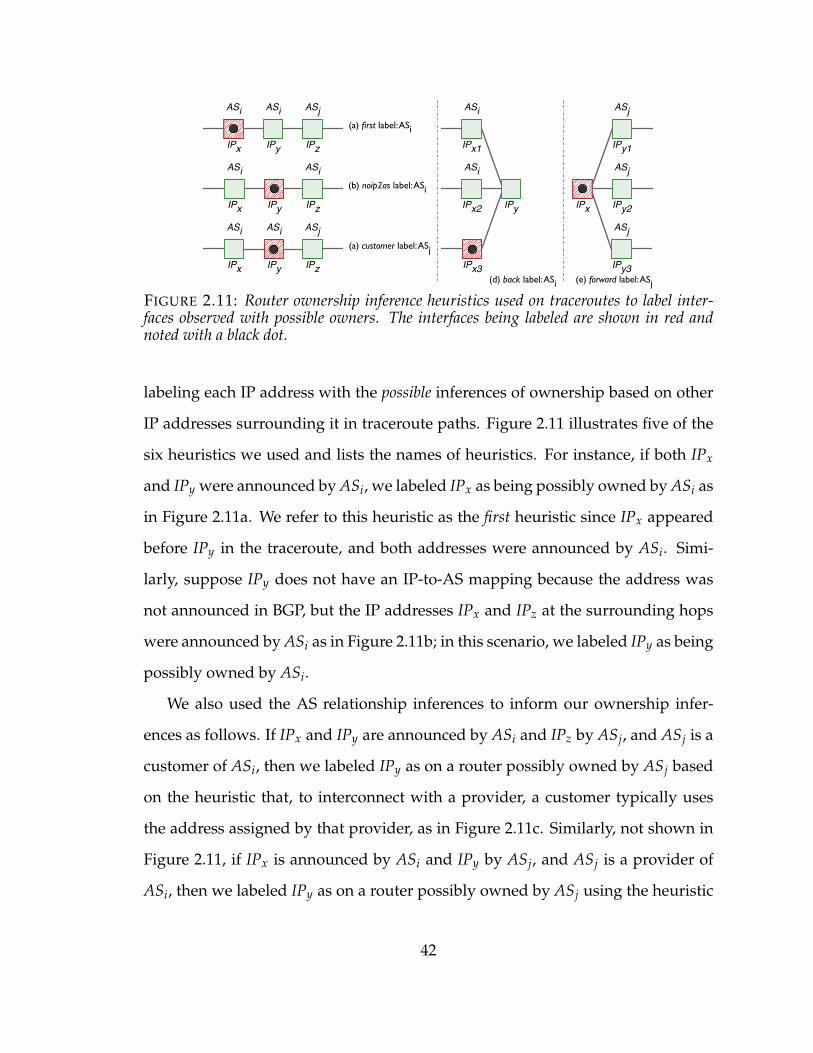
ASi

IPx

ASi

IPy

ASj

IPz

ASi

IPx

ASi

IPzIPy

ASi

IPx

ASj

IPz

ASi

IPy

(a) first label: ASi

(b) noip2as label: ASi

(a) customer label: ASj

ASi

IPx1

IPx3

ASi

IPx2 IPy

(d) back label: ASi (e) forward label: ASj

ASj

IPy1

ASj

IPy3

ASj

IPy2IPx

FIGURE 2.11: Router ownership inference heuristics used on traceroutes to label inter-faces observed with possible owners. The interfaces being labeled are shown in red andnoted with a black dot.

labeling each IP address with the possible inferences of ownership based on other

IP addresses surrounding it in traceroute paths. Figure 2.11 illustrates five of the

six heuristics we used and lists the names of heuristics. For instance, if both IPx

and IPy were announced by ASi, we labeled IPx as being possibly owned by ASi as

in Figure 2.11a. We refer to this heuristic as the first heuristic since IPx appeared

before IPy in the traceroute, and both addresses were announced by ASi. Simi-

larly, suppose IPy does not have an IP-to-AS mapping because the address was

not announced in BGP, but the IP addresses IPx and IPz at the surrounding hops

were announced by ASi as in Figure 2.11b; in this scenario, we labeled IPy as being

possibly owned by ASi.

We also used the AS relationship inferences to inform our ownership infer-

ences as follows. If IPx and IPy are announced by ASi and IPz by ASj, and ASj is a

customer of ASi, then we labeled IPy as on a router possibly owned by ASj based

on the heuristic that, to interconnect with a provider, a customer typically uses

the address assigned by that provider, as in Figure 2.11c. Similarly, not shown in

Figure 2.11, if IPx is announced by ASi and IPy by ASj, and ASj is a provider of

ASi, then we labeled IPy as on a router possibly owned by ASj using the heuristic

42

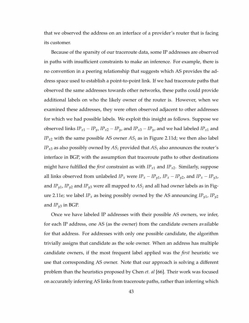
that we observed the address on an interface of a provider’s router that is facing

its customer.

Because of the sparsity of our traceroute data, some IP addresses are observed

in paths with insufficient constraints to make an inference. For example, there is

no convention in a peering relationship that suggests which AS provides the ad-

dress space used to establish a point-to-point link. If we had traceroute paths that

observed the same addresses towards other networks, these paths could provide

additional labels on who the likely owner of the router is. However, when we

examined these addresses, they were often observed adjacent to other addresses

for which we had possible labels. We exploit this insight as follows. Suppose we

observed links IPx1 ´ IPy, IPx2 ´ IPy, and IPx3 ´ IPy, and we had labeled IPx1 and

IPx2 with the same possible AS owner ASi as in Figure 2.11d; we then also label

IPx3 as also possibly owned by ASi provided that ASi also announces the router’s

interface in BGP, with the assumption that traceroute paths to other destinations

might have fulfilled the first constraint as with IPx1 and IPx2. Similarly, suppose

all links observed from unlabeled IPx were IPx ´ IPy1, IPx ´ IPy2, and IPx ´ IPy3,

and IPy1, IPy2 and IPy3 were all mapped to ASj and all had owner labels as in Fig-

ure 2.11e; we label IPx as being possibly owned by the AS announcing IPy1, IPy2

and IPy3 in BGP.

Once we have labeled IP addresses with their possible AS owners, we infer,

for each IP address, one AS (as the owner) from the candidate owners available

for that address. For addresses with only one possible candidate, the algorithm

trivially assigns that candidate as the sole owner. When an address has multiple

candidate owners, if the most frequent label applied was the first heuristic we

use that corresponding AS owner. Note that our approach is solving a different

problem than the heuristics proposed by Chen et. al [66]. Their work was focused

on accurately inferring AS links from traceroute paths, rather than inferring which

43

AS operates a given router.

With the inferences of AS owners of router IP addresses, we can then infer

whether a congested link is an internal link or interconnection and infer the link type

viz., provider-to-provider (p2p) and customer-to-provider (c2p). Because traceroutes

from more than one server pair can traverse the same link, it is possible for a link

to be marked as congested by more than one server-to-server pair—in some cases,

hundreds of server-to-server pairs.

In our study of IPv4 traceroutes, we identified 3155 IP-IP links to be respon-

sible for congestion. Of these around 1768 were internal links and 1121 were in-

terconnection links. Note, however, that it is possible to misidentify a number of

interconnection links as internal. Of the 1121 interconnection links, we identified

658 to be p2p and 463 to be c2p. For the remaining 266 links it was not possible

to infer if the link was an internal or interconnection link. Thus a higher number

of internal links are detected to be congested as compared with interconnection

links. However, when we weight the links by the number of server-to-servers

paths that cross them, we find that the interconnection links are more popular.

The large majority of the interconnection links with congestion were private in-

terconnects. In our datasets around 60 links that were established over the public

switching fabric of IXPs experienced congestion. This is not surprising since most

IXPs have strict service level agreements (SLAs) concerning the peak utilization

level and duration of the switch port used by the members; for instance, refer to

the SLA of one of the largest IXPs AMS-IX in Amsterdam [35]. Thus, we expect

that significant congestion occurs in cross-connects.

2.8.4 Estimating Congestion Overhead

In Figure 2.12 we present the overhead due to the congestion in our data set. For

both internal and interconnection links the typical overhead is between 20 ms and

44

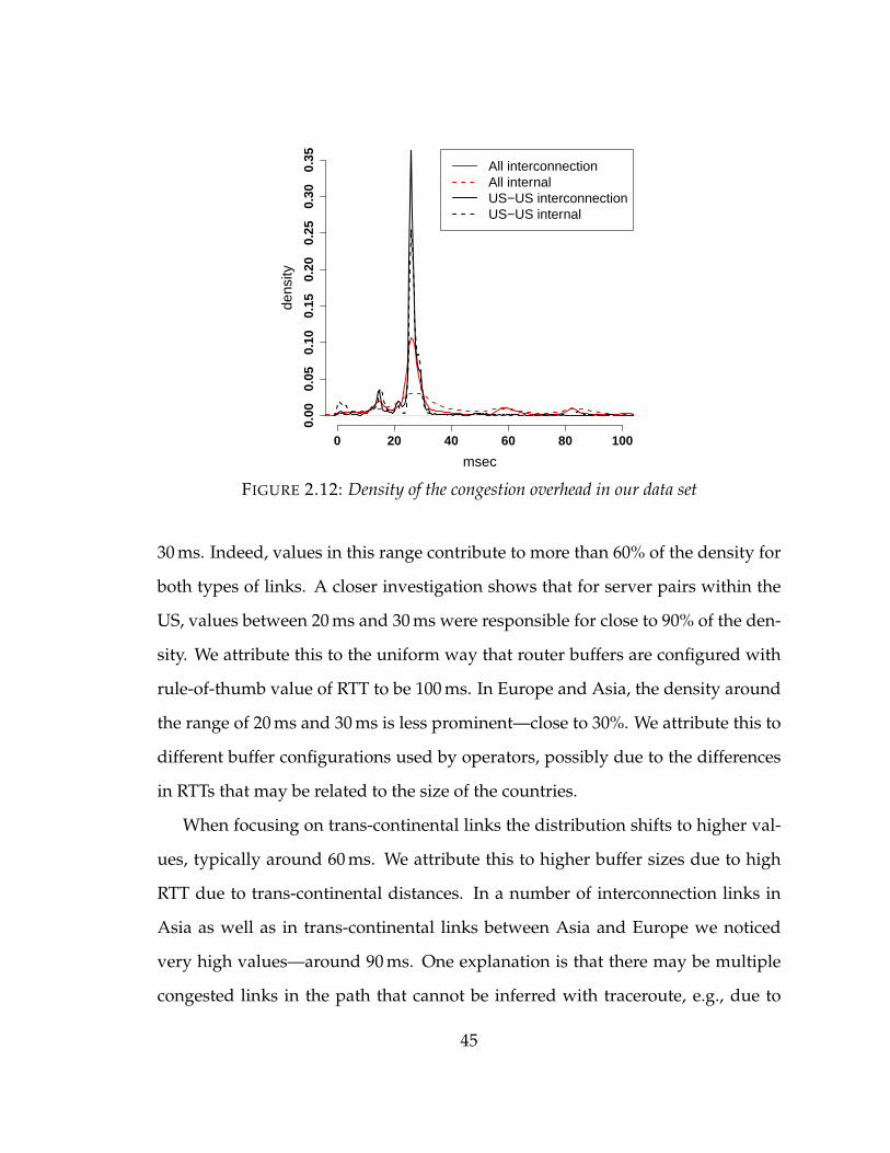
msec

dens

ity

0 20 40 60 80 100

0.00

0.05

0.10

0.15

0.20

0.25

0.30

0.35

All interconnectionAll internalUS−US interconnectionUS−US internal

FIGURE 2.12: Density of the congestion overhead in our data set

30 ms. Indeed, values in this range contribute to more than 60% of the density for

both types of links. A closer investigation shows that for server pairs within the

US, values between 20 ms and 30 ms were responsible for close to 90% of the den-

sity. We attribute this to the uniform way that router buffers are configured with

rule-of-thumb value of RTT to be 100 ms. In Europe and Asia, the density around

the range of 20 ms and 30 ms is less prominent—close to 30%. We attribute this to

different buffer configurations used by operators, possibly due to the differences

in RTTs that may be related to the size of the countries.

When focusing on trans-continental links the distribution shifts to higher val-

ues, typically around 60 ms. We attribute this to higher buffer sizes due to high

RTT due to trans-continental distances. In a number of interconnection links in

Asia as well as in trans-continental links between Asia and Europe we noticed

very high values—around 90 ms. One explanation is that there may be multiple

congested links in the path that cannot be inferred with traceroute, e.g., due to

45

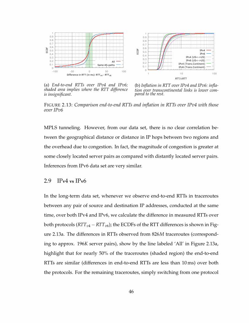
0 0.1 0.2 0.3 0.4 0.5 0.6 0.7 0.8 0.9

1

-100 -50 0 50 100

ECDF

Difference in RTT (in ms): RTTv4 - RTTv6

AllSame AS-paths

(a) End-to-end RTTs over IPv4 and IPv6;shaded area implies where the RTT differenceis insignificant.

0 0.1 0.2 0.3 0.4 0.5 0.6 0.7 0.8 0.9

1

1 10 100

ECDF

RTT/cRTT

IPv4IPv6

IPv4 (US<->US)IPv6 (US<->US)

IPv4 (Trans.Continent)IPv6 (Trans.Continent)

(b) Inflation in RTT over IPv4 and IPv6: infla-tion over transcontinental links is lower com-pared to the rest.

FIGURE 2.13: Comparison end-to-end RTTs and inflation in RTTs over IPv4 with thoseover IPv6

MPLS tunneling. However, from our data set, there is no clear correlation be-

tween the geographical distance or distance in IP hops between two regions and

the overhead due to congestion. In fact, the magnitude of congestion is greater at

some closely located server pairs as compared with distantly located server pairs.

Inferences from IPv6 data set are very similar.

2.9 IPv4 vs IPv6

In the long-term data set, whenever we observe end-to-end RTTs in traceroutes

between any pair of source and destination IP addresses, conducted at the same

time, over both IPv4 and IPv6, we calculate the difference in measured RTTs over

both protocols (RTTv4´RTTv6); the ECDFs of the RTT differences is shown in Fig-

ure 2.13a. The differences in RTTs observed from 826M traceroutes (correspond-

ing to approx. 196K server pairs), show by the line labeled ‘All’ in Figure 2.13a,

highlight that for nearly 50% of the traceroutes (shaded region) the end-to-end

RTTs are similar (differences in end-to-end RTTs are less than 10 ms) over both

the protocols. For the remaining traceroutes, simply switching from one protocol

46

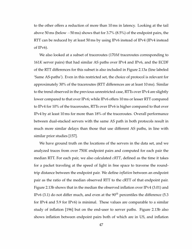
to the other offers a reduction of more than 10 ms in latency. Looking at the tail

above 50 ms (below ´50 ms) shows that for 3.7% (8.5%) of the endpoint pairs, the

RTT can be reduced by at least 50 ms by using IPv6 instead of IPv4 (IPv4 instead

of IPv6).

We also looked at a subset of traceroutes (170M traceroutes corresponding to

161K server pairs) that had similar AS paths over IPv4 and IPv6, and the ECDF

of the RTT differences for this subset is also included in Figure 2.13a (line labeled

‘Same AS-paths’). Even in this restricted set, the choice of protocol is relevant for

approximately 30% of the traceroutes (RTT differences are at least 10 ms). Similar

to the trend observed in the previous unrestricted case, RTTs over IPv4 are slightly

lower compared to that over IPv6; while IPv6 offers 10 ms or lesser RTT compared

to IPv4 for 10% of the traceroutes, RTTs over IPv6 is higher compared to that over

IPv4 by at least 10 ms for more than 18% of the traceroutes. Overall performance

between dual-stacked servers with the same AS path in both protocols result in

much more similar delays than those that use different AS paths, in line with

similar prior studies [157].

We have ground truth on the locations of the servers in the data set, and we

analyzed traces from over 750K endpoint pairs and computed for each pair the

median RTT. For each pair, we also calculated cRTT, defined as the time it takes

for a packet traveling at the speed of light in free space to traverse the round-

trip distance between the endpoint pair. We define inflation between an endpoint

pair as the ratio of the median observed RTT to the cRTT of that endpoint pair.

Figure 2.13b shows that in the median the observed inflation over IPv4 (3.01) and

IPv6 (3.1) do not differ much, and even at the 90th percentiles the difference (5.3

for IPv4 and 5.9 for IPv6) is minimal. These values are comparable to a similar

study of inflation [196] but on the end-user to server paths. Figure 2.13b also

shows inflation between endpoint pairs both of which are in US, and inflation

47

where the path between endpoint pairs (connecting US and Germany, or US and

Australia, or US and India, or US and Japan) involves transcontinental links. Not

surprisingly, in our data, inflation involving transcontinental links is significantly

lower compared to inflation between endpoints pairs in the US.

While Singla et al. [196] geolocated the end-users for computing the RTT infla-

tion, which can affect the results (depending on the accuracy of the geolocation),

we have ground truth on locations of servers, and we also compare the inflation in

RTT between the endpoints over both IPv4 and IPv6. The inflation shown in Fig-

ure 2.13b is based only on end-to-end RTTs between servers and hence, inflation

in the core most likely stem from infrastructure inefficiencies; for instance, there

are no DNS lookups or TCP handshakes involved in these calculations.

2.10 Discussion

Using server-to-server paths as a proxy to the Internet’s core, we show that con-

gestion is not the norm in the Internet’s core and also that routing changes, for

the most part, do not significantly affect the end-to-end RTTs. Studies [225] have

shown that when the RTTs of end-user-to-server paths increase significantly, a

significant fraction of such instances can be attributed to routing changes. In the

context of server-to-server paths, our results confirm, however, that the converse

is not true: routing changes only rarely have a significant impact on the end-to-

end RTTs of paths.

A natural question to ask is whether the non-typical cases are more prevalent

for routing or congestion. Although we do not have an ideal side-by-side compar-

ison, our results suggest that routing changes have the greater impact. Figure 2.9

on routing shows that for 10% of trace timelines the (sub-optimal) AS paths that

led to at least 20 ms increase in RTTs pertained for at least 30% of the study period

48

for IPv4 and 50% for IPv6. In contrast, in Section 2.8 on congestion, just 2% (much

less than 10%) of the server pairs over IPv4, and just 0.6% over IPv6, experience a

strong diurnal pattern with an increase in RTT of least 10 ms. It is, nevertheless,

possible that in case of a particular server pair congestion might be the greater

issue.

Prior studies have shown that having control of both endpoints of a commu-

nication channel, as in the case of server-to-server communications, offers great

benefits; for instance, proprietary protocols can be deployed with minimal effort

to deal with the pathologies of TCP [87, 160]. Through this study, we report on

two additional characteristics of server-to-server communications: (1) server-to-

server paths are consistent, suffering little or no change at the AS level, and (2)

routing changes and consistent congestion, in the core, typically do not affect the

end-to-end RTTs of the server-to-server paths. Based on our study, the behavior of

the server-to-server landscape is in stark contrast with that of other segments of

the Internet, e.g., access networks. Performance of access networks, for instance,

typically experience time-of-day effects, exhibiting poor performance during the

peak hours [203, 173].

We show that there is hardly any difference in end-to-end latency for close to

70% of traceroutes that use the same AS paths over IPv4 and IPv6. Our longitudi-

nal study strongly endorses transitioning to IPv6. Citing latency penalty incurred

due to use of IPv6 is no longer a feasible excuse, at least not in the Internet’s core,

to delay IPv6 adoption. Even when latency over both protocols is not similar, us-

ing dual-stack deployments to carefully switch from one protocol to the other can

yield substantial performance gains. IPv6 is faster than IPv4 in at least 10% of the

traceroutes in our longitudinal study. Latency penalties incurred by forcing use of

IPv4, in the core, all the time can impact end-users’ experience; latency penalties

in the core may have a multiplicative effect on end-to-end latencies [196].

49

Studies of known peering disputes [138] show that congestion of particular

links that run “hot” experience unusually high delays, but the congestion disap-

pears in a few hours after agreements to settle the disputes. These emphasize the

highly variable nature of the Internet’s core necessitating continuous monitoring

over longer time periods for accurate evaluations. Our work is an example of such

a continuous monitoring over a period of 16-months.

The observed performance characteristics may be due to the structural changes

in Internet’s core, also referred to as “flattening of the Internet” [187, 77, 22], or the

increase of peering locations [63, 64], or the pressure on transit providers to offer

cheaper and competitive service [134], or investments in alternative high-speed

networks [196], or the deployment of the massively distributed server infrastruc-

tures [49, 116, 160, 154, 23]; it is hard to pin-point the exact root cause without

further studies.

An understandable criticism is that the view of the Internet’s core from the

perspective of a service provider may be different than that of other networks, e.g.,

eyeball, transit. Indeed, it is possible that measurements from other platforms,

viz., Dasu [188], iPlane [141], may offer a different view of the Internet’s core. Such

studies will complement our work and aid in finding the exact root causes behind

the observations. Other performance characteristics such as the available capacity

in the Internet’s core [27] should also be revisited given the recent changes in the

Internet ecosystem.

2.11 Summary

With the adoption of the cloud computing paradigm, server-to-server interactions

have become a key determinant in the realization of cloud services. Latencies in

the core may impact end-users’ experience and affect monetization of cloud ser-

50

vices. We exploit a large corpus of measurements in both forward and reverse

directions between thousands of CDN servers, and, using the server-to-server

landscape as a proxy to the Internet’s core, offer insights into the performance

characteristics of the core. Our data suggests that significant daily oscillations in

latency, herein called congestion, is not the norm in the Internet’s core. However,

at times, some links do experience congestion, and we detected such incidents on

a greater number of internal links than interconnection links. When we weight

the links by the number of server-to-servers paths that cross them, we find that

the interconnection links are more popular. The large majority of the interconnec-

tion links with congestion were private interconnects. We also show that while

routing changes typically have marginal or no impact on the end-to-end RTTs, 4%

(7%) of routing changes on IPv4 (IPv6) increase RTTs by at least 50 ms for at least

20% of the study period. The non-typical cases affecting RTTs are more prevalent

for routing than congestion.

It is imperative to understand the ramifications of cloud computing on state of

the Internet’s core. In this regard, our work on the back-office traffic only scratches

the surface, and highlights the need for more studies of the server-to-server land-

scape. Our longitudinal study, further, focuses only on the latencies in the Inter-

net’s core. We encourage follow-up work focusing on other characteristics, viz.,

available bandwidth, packet loss, and utilizing other measurement platforms to

further enrich our understanding of the Internet’s core. The similarity in perfor-

mance characteristics over IPv4 and IPv6 also calls for a study to understand to

what extent infrastructure is shared between IPv4 and IPv6, and we plan on ad-

dressing this question in future work.

51

3

Failures as a First-class Citizen

Most software today is very much like an Egyptian pyramidwith millions of bricks piled on top of each other, with no

structural integrity, but just done by brute force and thousandsof slaves.

— Alan KayACM A.M. Turing Award Winner 2003

Software-defined networking (SDN) decouples the control plane from the data

plane, and offers a simple, centralized view to programmatically manage the

data plane. SDN has indeed revolutionized the way we manage our networks:

many of the biggest names in the industry, e.g., Google [131, 15, 17, 116], Mi-

crosoft [199, 100], Facebook, Amazon, extensively employ SDN-based solutions

to manage their cloud infrastructure. Today, the SDN ecosystem boasts of a rich

diversity of SDN controllers and innovative control applications (SDN-Apps); en-

terprise network operators can build customized solutions and deploy them with

ease. The SDN approach virtually marginalizes the traditional (or manual) error-

prone network management tasks. But bugs are endemic in software and SDN-

Apps are no exception.

A key appeal of SDN lies in its ability to enable innovative control applica-

52

tions (SDN-Apps). These SDN-Apps contain sophisticated code to interface with

increasingly complicated controller code-bases and to interoperate with complex

and, often, buggy switches [126]. The end-result of these complexities is that SDN-

Apps are prone to a variety of bugs (e. g., timing bugs [52, 172], or null pointers).

The SDN-Apps, furthermore, are likely to be provided with limited testing by

third party entities—a trend that is expected to become more prevalent given the

recent success of open-source controllers, e. g., OpenDaylight [16], and the emer-

gence of SDN app stores, e. g., HP’s SDN App Store [18].

Recent efforts to improve the reliability of SDN-Apps and availability of the

SDN controller have been along three directions: first, diagnosing and pinpoint-

ing the root cause of failures [52, 190]; second, attacking the root cause of failures

by providing better programming abstractions for developers [172, 51]; and third,

developing better fault-recovery techniques through controller replication [118,

125, 219]. Of the three, only the last direction enables the SDN controller to recover

from SDN-App failures in production networks. In case of controller replication,

multiple replicas of the controller are deployed with each replica maintaining a

state machine. Events are input to all the replicas in the same order, thus keeping

all state machines identical to one another. One of the replicas is designated as

the leader (or master), and when the master fails, a different replica can transpar-

ently take over and resume control of the SDN-Apps and the network. Controller

replication, however, does not offer much help, when the crash of the SDN-App

is caused by deterministic bugs.

There is a rich literature on the topic of fault tolerance, with studies address-

ing the issue in different contexts and particularly, distributed systems, operat-

ing systems and application servers. Direct application of these well-researched

techniques to the problem of making controllers fault-tolerant to SDN-App fail-

ures, nevertheless, is not feasible. Techniques like reboot [50] or replay [207], for

53

instance, cannot be applied directly to the SDN control plane; certain fundamen-

tal assumptions made by these techniques do not hold true in an SDN environ-

ment. Both the network and SDN-Apps, moreover, contain state, and reboot-

ing [50] the SDN-App (after a crash) will eliminate this state and consequently, in-

troduce inconsistency issues. Further, if the crash was due to deterministic bugs,

replaying events [207, 177, 185] to restore the SDN-App’s state will be stuck in a

never-ending crash-and-reboot loop. In addition, attempts to tackle deterministic

bugs [177, 185] tend to change the application’s environment and may introduce

erroneous output [185].

A key feature of SDNs is the clean, narrow and open application program-

ming interface (API) that is used for communication between the data and control

planes. This feature differentiates SDN’s fault tolerance from traditional OS fault

tolerance wherein little is known about the semantics of the messages that the ap-

plication processes. Using the API’s specification, we can extract the semantics

of the API and understand the intent of each message or event. Further, we can

exploit this knowledge to develop recovery mechanisms that can make modifica-

tions to the SDN-App code, environment, and/or its input without violating the

semantics of the SDN-App code.

There are a number of challenges in safely recovering SDN-Apps from fail-

ures. First, network state is manipulated and shared by many SDN-Apps; a state-

ful SDN-App internally maintains a subset of the network state, which reflects

its view of the network. Given this replicated state across stateful SDN-Apps, a

key challenge lies in maintaining a consistent network state across the different

SDN-Apps during failure recovery. Second, although, the semantics of the SDN

control messages are well-specified and well-documented, no protocols exist to

exploit this information for designing a better recovery mechanism. Determining

how to leverage the semantic knowledge of the protocol in improving recovery

54

mechanisms is also a hard problem. Third, the monolithic design of current SDN

controllers implies that a failure of any one component renders the entire con-

trol plane unavailable [58]. There is a need, consequently, for a better isolation

between the different components.

In this chapter, we take a bold step towards developing a fault-tolerant con-

troller architecture, called LegoSDN, that explicitly aims to safely recover SDN-

Apps from both deterministic and non-deterministic failures. LegoSDN builds on

the well-defined abstractions [58] to develop a hierarchy of event transformations,

and to add support for transactions that cut across data and control planes. We

present a prototype implementation that isolates the SDN-Apps from one another

and from the controller by running each within a sandbox; failure of an SDN-App

is restricted to the sandbox in which it is run. The interactions between the con-

troller and SDN-Apps are carried out via remote procedure calls (RPC).

LegoSDN tackles the challenge of maintaining consistency across different SDN-

Apps by employing fine-grained transactional semantics spanning both the data

and control planes, and thereby enabling the controller to rollback changes made

by a crashing SDN-App without impacting other (healthy) SDN-Apps. The trans-

actional semantics, moreover, include conflict detection and resolution to main-

tain consistency between the SDN-Apps.

LegoSDN employs novel domain-specific transformations that modify crash-

inducing events into semantically equivalent, but syntactically different, events to

safely recover a crashed SDN-App. These transformed events are then replayed to

the SDN-App restored from the crash. The transform-and-replay process contin-

ues until the SDN-App can process the transformed events successfully (without

crashing). The system also provides a framework for searching through the space

of equivalent events and automating this transform-and-replay process.

As a proof-of-concept, we re-architected the Floodlight controller to support

55

LegoSDN. Using this prototype, we demonstrate that LegoSDN imposes minimal

overheads and requires no modifications to the SDN-Apps (designed to run us-

ing Floodlight), thus shielding SDN-App developers from having to spend time

learning the complexities of LegoSDN. Using a synthetic fault injector to crash-test

SDN-Apps and using mininet [128] for emulating a network topology, we evalu-

ated LegoSDN using five different SDN-Apps by exploring the time to recovery

and by analyzing the implications of maintaining consistency.

Our contributions can be summarized as follows.

• Cross-Layer Transaction Manager: We propose a framework to provide

transactional semantics across both control and data planes; this framework

allows us to isolate failures and maintain consistency by rolling back changes

made by failed SDN-Apps without requiring hardware changes to the switches

(§3.4).

• SDN Event Transformer: We present a protocol for overcoming determinis-

tic failures by extending traditional log-replay-based techniques to include

domain-specific transformations that preserve the SDN-App semantics (in-

tent and meaning) (§3.5).

• Implementation and Evaluation: We build a working prototype of a con-

troller architecture that implements our primitives in Floodlight.

3.1 Acknowledgments

This chapter is based on a joint work with Theophilus Benson and Brendan Tschaen.

We presented first an outline of the ideas discussed in this chapter as a position

paper, “Tolerating SDN Application Failures with LegoSDN” [57], and followed

it with a publication that included a prototype implementation and comparative

evaluations to demonstrate the validity of our ideas.

56

3.2 Motivation

In this section, we review the state of the SDN ecosystem (§3.2.1) and describe the

issues posed by SDN-App crashes1 (§3.2.2). We, then, highlight the challenges in

recovering SDN-Apps from crashes (§3.2.4) and outline the design goals (§3.2.5)

of a fault-tolerant controller architecture.

3.2.1 State of the SDN Ecosystem

The SDN ecosystem has witnessed tremendous growth over the last decade with

some of the biggest names in the technology sector, e.g., Google, Microsoft, em-

bracing SDN-based solutions to manage their infrastructures [131, 199]. In the

realm of enterprise networking, numerous startups, e.g., Veriflow [19], PLUM-

grid [14], Big Switch Networks [13] have emerged with innovative SDN-Apps.

Today, enterprise SDN adopters have a rich selection of SDN controllers—Open

Daylight [16], Floodlight [42], Ryu [70], POX [182], NOX [181]—and an even richer

set of options for SDN-Apps from different software vendors.

Indeed, enterprises, today, can mix and match SDN controllers and SDN-Apps

from different vendors. We list a few SDN-Apps in Table 3.1, briefly describe

their purpose, and indicate whether they are third-party SDN-Apps. A third-party

SDN-App implies that the SDN-App is developed by a software vendor which is

different from that of the SDN controller (with which the SDN-App is designed

to run). The Virtual Tenant Network (VTN) [150] from NEC [9], for instance,

is a third-party SDN-App designed to run with the SDN controller from Open

Daylight [16]. On the other hand, the BigTap [3] SDN-App and the Floodlight

SDN controller with which it runs are both developed by Big Switch Networks,

Inc. [13]; hence, the designation of in house under the Developer column for this

1 The terms ‘crash’, ‘fault’, and ‘failures’ are used interchangeably, and refer to abrupt terminationof the SDN-App, unless otherwise mentioned.

57

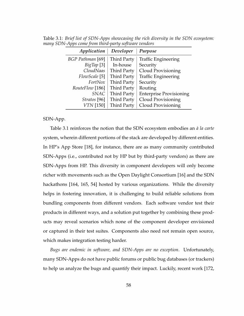
Table 3.1: Brief list of SDN-Apps showcasing the rich diversity in the SDN ecosystem:many SDN-Apps come from third-party software vendors

Application Developer Purpose

BGP Pathman [69] Third Party Traffic EngineeringBigTap [3] In-house Security

CloudNaas Third Party Cloud ProvisioningFlowScale [5] Third Party Traffic Engineering

FortNox Third Party SecurityRouteFlow [186] Third Party Routing

SNAC Third Party Enterprise ProvisioningStratos [96] Third Party Cloud ProvisioningVTN [150] Third Party Cloud Provisioning

SDN-App.

Table 3.1 reinforces the notion that the SDN ecosystem embodies an à la carte

system, wherein different portions of the stack are developed by different entities.

In HP’s App Store [18], for instance, there are as many community contributed

SDN-Apps (i.e., contributed not by HP but by third-party vendors) as there are

SDN-Apps from HP. This diversity in component developers will only become

richer with movements such as the Open Daylight Consortium [16] and the SDN

hackathons [164, 165, 54] hosted by various organizations. While the diversity

helps in fostering innovation, it is challenging to build reliable solutions from

bundling components from different vendors. Each software vendor test their

products in different ways, and a solution put together by combining these prod-

ucts may reveal scenarios which none of the component developer envisioned

or captured in their test suites. Components also need not remain open source,

which makes integration testing harder.

Bugs are endemic in software, and SDN-Apps are no exception. Unfortunately,

many SDN-Apps do not have public forums or public bug databases (or trackers)

to help us analyze the bugs and quantify their impact. Luckily, recent work [172,

58

190, 52] on debugging SDN-Apps have uncovered a number of interesting bugs in

the SDN-Apps for Floodlight [42], POX [182], and NOX [181] controllers. Further,

a cursory examination of the Open Daylight bug repository shows that bugs are

present, unsurprisingly, even in the SDN-Apps that come bundled (i.e., developed

in-house) with the controller. While novel abstractions [51] are being developed

to minimize the number of bugs, there’s no silver bullet for eliminating bugs. Ex-

tensive studies on software-engineering practices indicate that bugs are prevalent

in most applications, and that most bugs in production quality code do not even

have fixes [218]. In an SDN network, bugs in an SDN-App can bring down the

entire SDN stack [58, 195].

3.2.2 SDN-App Failure Scenarios

SDN-Apps are designed typically to be event-driven2 with the implementation

comprising event handlers for different inputs or network events, e.g., link acti-

vation (link-up) or switch failures (switch-down). Anecdotal evidences [172, 52],

unsurprisingly, suggest that most of the bugs reside in these event handlers. We

focus, hence, on these event handlers of the SDN-Apps.

Failures resulting from the bugs in SDN-Apps can be broadly classified into

two types—fail-stop failures and invariant violations. Fail-stop failures are those

where the SDN-App terminates unexpectedly due to invalid memory accesses

(e.g., null-pointer dereferences) or evaluation of erroneous expressions (e.g., divi-

sion by zero). Invariant violations refer to scenarios where the SDN-App installs a

set of OpenFlow rules that violate a network invariant, e.g., creating a loop or creat-

ing a black hole. Fail-stop bugs will bring down the entire SDN controller, because

of the lack of isolation between the SDN-App and the controller, while invariant

violations introduce inconsistencies (or policy violations) in the network.

2 Traditional control-plane applications, e.g., OSPF, Spanning Tree, are similarly event-driven.

59

Although techniques exist [124, 195, 118] to detect and potentially isolate these

failures, they offer little help once an SDN-App encounters a failure. These tech-

niques cannot safely recover the SDN-App, and,in particular, there are very few

tools for recovering SDN-Apps from deterministic failures.

3.2.3 Implications of SDN-App Failures

Cascading fail-stop failures can cripple the entire SDN stack, since crash of the

controller translates often loss of network control. OpenFlow switches can be

configured to operate either in fail-open mode or fail-close mode. When config-

ured in fail-open mode the switches default to performing traditional ethernet-

based switching when the controller is unavailable. In case a fail-stop failure,

switches operating in fail-open mode can result in violations of network policies

(e.g., security requirements, service-level agreements (SLAs)). In fail-close mode,

the switches effectively do nothing when the controller fails, and network control

is lost until the SDN stack is rebooted. In an SDN environment, both the control

plane and the data plane may maintain state (e.g., topology information, flow-

level statistics). Fail-stop failures can result in the loss of this state, introducing

network inconsistencies, as a consequence. Rebooting the SDN stack, hence, is

often not a feasible solution, when the lost state cannot be safely recovered.

The network is a shared substrate—multiple SDN-Apps may configure the same

set of network devices in different (non-conflicting3) ways to implement differ-

ent network policies. The network policies often require atomic configuration of

several network devices; but the mechanisms for enforcing these policies are not

atomic. For instance, in Figure 3.1a, App1 modifies three switches on the network

to setup a path for a flow. App1, however, may fail midway (Figure 3.1b) dur-

3 We assume non-conflicting behavior, since the alternative is disastrous even in the absence ofbugs or failures.

60

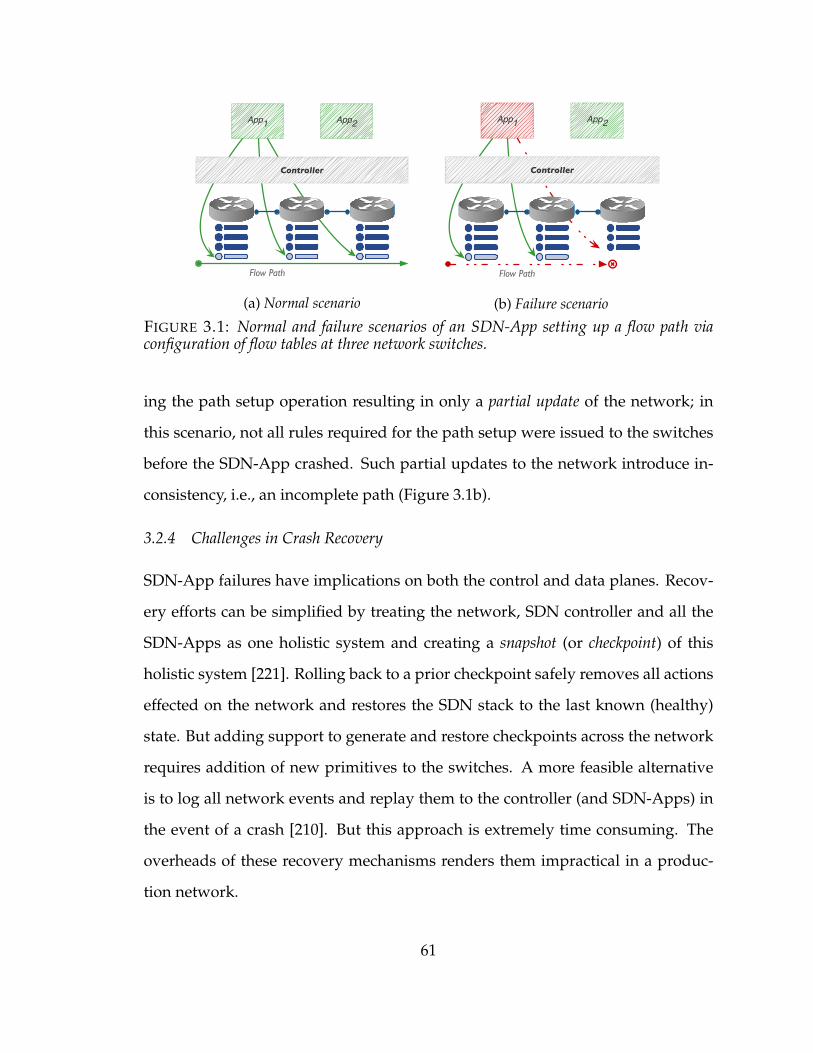
Controller

App1 App2

Flow Path

(a) Normal scenario

App1

Controller

App2

Flow Path

(b) Failure scenario

FIGURE 3.1: Normal and failure scenarios of an SDN-App setting up a flow path viaconfiguration of flow tables at three network switches.

ing the path setup operation resulting in only a partial update of the network; in

this scenario, not all rules required for the path setup were issued to the switches

before the SDN-App crashed. Such partial updates to the network introduce in-

consistency, i.e., an incomplete path (Figure 3.1b).

3.2.4 Challenges in Crash Recovery

SDN-App failures have implications on both the control and data planes. Recov-

ery efforts can be simplified by treating the network, SDN controller and all the

SDN-Apps as one holistic system and creating a snapshot (or checkpoint) of this

holistic system [221]. Rolling back to a prior checkpoint safely removes all actions

effected on the network and restores the SDN stack to the last known (healthy)

state. But adding support to generate and restore checkpoints across the network

requires addition of new primitives to the switches. A more feasible alternative

is to log all network events and replay them to the controller (and SDN-Apps) in

the event of a crash [210]. But this approach is extremely time consuming. The

overheads of these recovery mechanisms renders them impractical in a produc-

tion network.

61

Anecdotal evidences suggest that the most common failures are due to a com-

bination of unexpected timing and concurrency issues [172]. Regardless, these

errors are often deterministic in nature and simply replaying the events in the

same order will be insufficient. For example, the concurrency bugs tackled in

OF.CPP [172] are deterministic and require more advanced techniques than sim-

ple reboot [50] or log-replay [210]. Many of these bugs require some transfor-

mation of the failure-inducing message(s); these can be simple transformations,

e.g., reordering, to solve the concurrency related errors [172, 52], or more complex

transformations involving modifications to the messages or deletions of a subset

of messages to tackle other issues.

A key challenge in transforming messages is in ensuring that the transformed

events maintain protocol equivalence with the original input messages. More con-

cretely, the transformations performed should retain the semantic intent of the

original messages while adhering to the protocol specification. Fortunately, Open-

Flow events are well-documented and their semantics are clearly defined in the

OpenFlow specification. We can extract the intent and meaning of each message

using the OpenFlow specification, and use this information to create a set list of

potential transformations for each event or message. This effort represents a one-

time cost that can be shared across various controllers and SDN-Apps.

3.2.5 Design Goals

We can summarize our observations as follows: failures in SDN-Apps are, typi-

cally, deterministic in nature and require recovery mechanisms that are more so-

phisticated compared to checkpoint-restore or reboot (and replay); the semantics

of SDN events (or control messages) are well-known and can be used to create a

list of event-specific transformations to provide for safe recovery of SDN-Apps,

particularly in case of deterministic faults; safe recovery entails maintaining con-

62

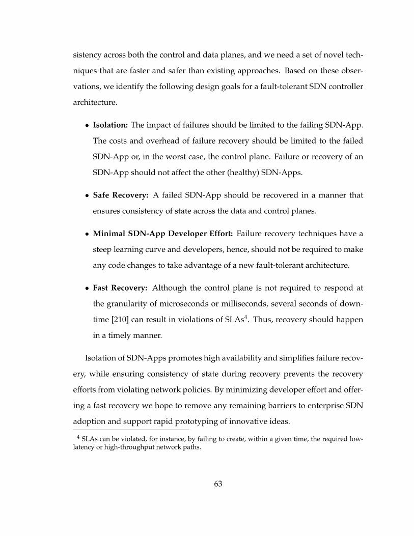
sistency across both the control and data planes, and we need a set of novel tech-

niques that are faster and safer than existing approaches. Based on these obser-

vations, we identify the following design goals for a fault-tolerant SDN controller

architecture.

• Isolation: The impact of failures should be limited to the failing SDN-App.

The costs and overhead of failure recovery should be limited to the failed

SDN-App or, in the worst case, the control plane. Failure or recovery of an

SDN-App should not affect the other (healthy) SDN-Apps.

• Safe Recovery: A failed SDN-App should be recovered in a manner that

ensures consistency of state across the data and control planes.

• Minimal SDN-App Developer Effort: Failure recovery techniques have a

steep learning curve and developers, hence, should not be required to make

any code changes to take advantage of a new fault-tolerant architecture.

• Fast Recovery: Although the control plane is not required to respond at

the granularity of microseconds or milliseconds, several seconds of down-

time [210] can result in violations of SLAs4. Thus, recovery should happen

in a timely manner.

Isolation of SDN-Apps promotes high availability and simplifies failure recov-

ery, while ensuring consistency of state during recovery prevents the recovery

efforts from violating network policies. By minimizing developer effort and offer-

ing a fast recovery we hope to remove any remaining barriers to enterprise SDN

adoption and support rapid prototyping of innovative ideas.

4 SLAs can be violated, for instance, by failing to create, within a given time, the required low-latency or high-throughput network paths.

63

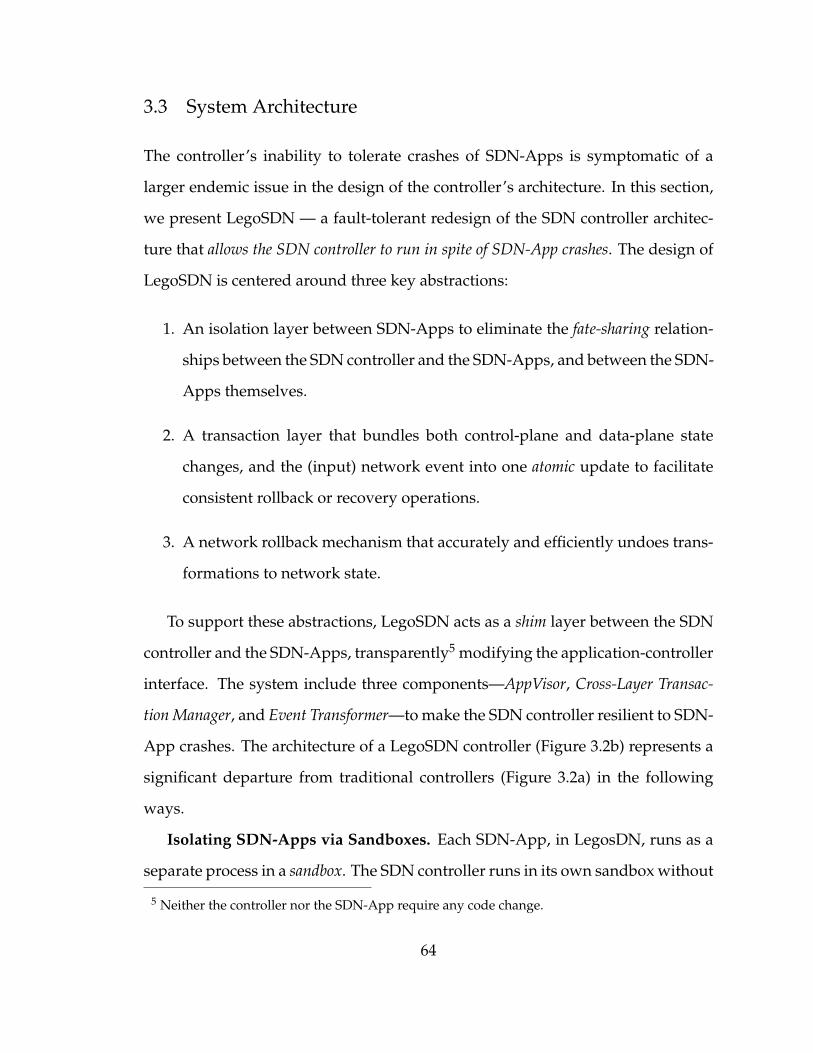
3.3 System Architecture

The controller’s inability to tolerate crashes of SDN-Apps is symptomatic of a

larger endemic issue in the design of the controller’s architecture. In this section,

we present LegoSDN — a fault-tolerant redesign of the SDN controller architec-

ture that allows the SDN controller to run in spite of SDN-App crashes. The design of

LegoSDN is centered around three key abstractions:

1. An isolation layer between SDN-Apps to eliminate the fate-sharing relation-

ships between the SDN controller and the SDN-Apps, and between the SDN-

Apps themselves.

2. A transaction layer that bundles both control-plane and data-plane state

changes, and the (input) network event into one atomic update to facilitate

consistent rollback or recovery operations.

3. A network rollback mechanism that accurately and efficiently undoes trans-

formations to network state.

To support these abstractions, LegoSDN acts as a shim layer between the SDN

controller and the SDN-Apps, transparently5 modifying the application-controller

interface. The system include three components—AppVisor, Cross-Layer Transac-

tion Manager, and Event Transformer—to make the SDN controller resilient to SDN-

App crashes. The architecture of a LegoSDN controller (Figure 3.2b) represents a

significant departure from traditional controllers (Figure 3.2a) in the following

ways.

Isolating SDN-Apps via Sandboxes. Each SDN-App, in LegosDN, runs as a

separate process in a sandbox. The SDN controller runs in its own sandbox without

5 Neither the controller nor the SDN-App require any code change.

64

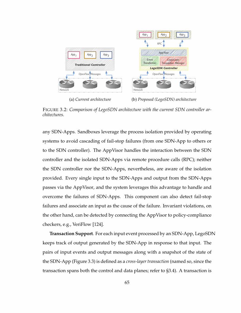
Traditional Controller

Network

App1 App2 App3

OpenFlow Messages

(a) Current architecture

LegoSDN Controller

Network

RPC

App1 App2 App3

OpenFlow Messages

App Visor

Event Transformer

Cross-Layer Transaction Manager

(b) Proposed (LegoSDN) architecture

FIGURE 3.2: Comparison of LegoSDN architecture with the current SDN controller ar-chitectures.

any SDN-Apps. Sandboxes leverage the process isolation provided by operating

systems to avoid cascading of fail-stop failures (from one SDN-App to others or

to the SDN controller). The AppVisor handles the interaction between the SDN

controller and the isolated SDN-Apps via remote procedure calls (RPC); neither

the SDN controller nor the SDN-Apps, nevertheless, are aware of the isolation

provided. Every single input to the SDN-Apps and output from the SDN-Apps

passes via the AppVisor, and the system leverages this advantage to handle and

overcome the failures of SDN-Apps. This component can also detect fail-stop

failures and associate an input as the cause of the failure. Invariant violations, on

the other hand, can be detected by connecting the AppVisor to policy-compliance

checkers, e.g., VeriFlow [124].

Transaction Support. For each input event processed by an SDN-App, LegoSDN

keeps track of output generated by the SDN-App in response to that input. The

pairs of input events and output messages along with a snapshot of the state of

the SDN-App (Figure 3.3) is defined as a cross-layer transaction (named so, since the

transaction spans both the control and data planes; refer to §3.4). A transaction is

65

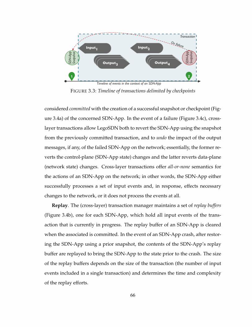
Transaction

Timeline of events in the context of an SDN-App

1

SDN

-App

Snap

shot

Input1

Msg OutxMsg OutxOutput3

Input2

Msg OutxMsg OutxOutput4

2

SDN

-App

Snap

shot

On failure

FIGURE 3.3: Timeline of transactions delimited by checkpoints

considered committed with the creation of a successful snapshot or checkpoint (Fig-

ure 3.4a) of the concerned SDN-App. In the event of a failure (Figure 3.4c), cross-

layer transactions allow LegoSDN both to revert the SDN-App using the snapshot

from the previously committed transaction, and to undo the impact of the output

messages, if any, of the failed SDN-App on the network; essentially, the former re-

verts the control-plane (SDN-App state) changes and the latter reverts data-plane

(network state) changes. Cross-layer transactions offer all-or-none semantics for

the actions of an SDN-App on the network; in other words, the SDN-App either

successfully processes a set of input events and, in response, effects necessary

changes to the network, or it does not process the events at all.

Replay. The (cross-layer) transaction manager maintains a set of replay buffers

(Figure 3.4b), one for each SDN-App, which hold all input events of the trans-

action that is currently in progress. The replay buffer of an SDN-App is cleared

when the associated is committed. In the event of an SDN-App crash, after restor-

ing the SDN-App using a prior snapshot, the contents of the SDN-App’s replay

buffer are replayed to bring the SDN-App to the state prior to the crash. The size

of the replay buffers depends on the size of the transaction (the number of input

events included in a single transaction) and determines the time and complexity

of the replay efforts.

66

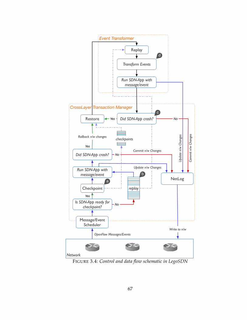
Event Transformer

CrossLayer Transaction Manager

Com

mit

n/w

Cha

nges

Upd

ate

n/w

Cha

nges

Network

Message/Event Scheduler

Checkpoint

Run SDN-App with message/event

NetLog

replay

Restore

Yes

Yes

No

Rollback n/w changes

Replay

Transform Events

Did SDN-App crash?

Write to n/w

OpenFlow Messages/Events

Run SDN-App with message/event

No

Did SDN-App crash?

a

c

d

b

checkpoints

Yes

NoCommit n/w Changes

Update n/w Changes

Is SDN-App ready for checkpoint?

FIGURE 3.4: Control and data flow schematic in LegoSDN

67

Safe Recovery. The Event Transformer component assists in recovering an

SDN-App from faults (in particular, deterministic faults). Rather than replaying

the messages available in the replay buffer, following a crash, the event trans-

former can transform an event (Figure 3.4d) to a different (but equivalent) event

that the SDN-App can, perhaps, process without encountering another crash. The

event transformer cycles through a set of predefined transformations for each

event until it finds the transformation that allows the recovered SDN-App to make

progress.

3.4 Cross-Layer Transactions

We define a cross-layer transaction as the state generated and/or modified in the

control and data planes as a result of an SDN-App processing one or more input

network events. More concretely, for a set of input events te1, e2, . . . , eNu processed

by an SDN-App, a cross-layer transaction is the set of variables tv1, v2, . . . , vnu that

changed within the SDN-App and the set of output messages to1, o2, . . . , onu sent

to the network. The variables make up the control-plane portion of the transaction

whereas the output messages to the network comprise the data-plane portion of

the transaction. The events te1, e2, . . . , eNu are the messages stored in the replay

buffer until the transaction containing them is committed. Cross-layer transac-

tions allows LegoSDN to perform a successful rollback of the SDN ecosystem to a

consistent state after a failure. In addition, these transactions ensure that the im-

plications of the failed SDN-App on the shared network substrate are not exposed

to the other (healthy) SDN-Apps.

Cross-layer transactions require support for the following three primitives:

• Cross-Layer Snapshots: Before an SDN-App begins a transaction, we have

to generate snapshots of the state of both the SDN-App and the network.

68

Checkpointing an SDN-App is relatively easy [71] compared to checkpoint-

ing network state since data plane devices currently lack appropriate primi-

tives to support the operation.

• Synchronized Rollback: In the event of a failure of an SDN-App, we have

to rollback the current (uncommitted) transaction, which implies undoing

changes effected by the SDN-App on the network. Rollback of changes to

the network, unsurprisingly, is quite challenging. While orthogonal state

management tools [201, 125] facilitate tracking of changes to the network,

none provide adequate primitives to support rollback.

• Data Plane Consistency: The network acts a shared substrate between dif-

ferent SDN-Apps, since network state may be shared among and manipu-

lated by many SDN-Apps. As a consequence, a naïve rollback of network

state, when an SDN-App fails, may introduce inconsistent state in other

(healthy) SDN-Apps. Hence, we need support for primitives to detect con-

flicts and systematically resolve them.

3.4.1 Snapshots

In LegoSDN, with AppVisor interposed between the SDN controller and the SDN-

Apps, the controller can easily checkpoint an SDN-App before triggering one of

its event handlers with an input. Creating checkpoints of the data plane, never-

theless, is hard since it requires modifications to the switch hardware [221, 83].

To eliminate the need for switch hardware changes, we introduce a (data-plane)

state-management layer to the controller. The state-management layer, imple-

mented by NetLog, models the data plane (or network) as a transactional sys-

tem. NetLog supports grouping of multiple actions (entries to be installed in flow

tables of switches) into one atomic operation (or update) and leverages existing

69

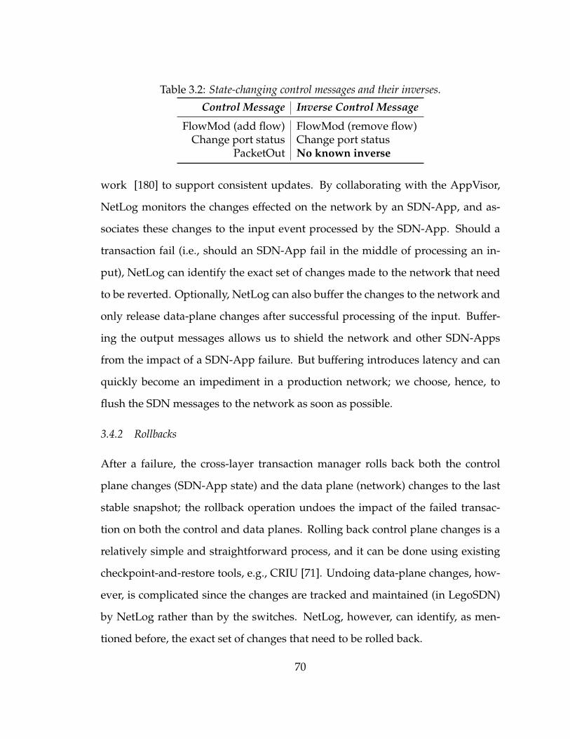
Table 3.2: State-changing control messages and their inverses.

Control Message Inverse Control Message

FlowMod (add flow) FlowMod (remove flow)Change port status Change port status

PacketOut No known inverse

work [180] to support consistent updates. By collaborating with the AppVisor,

NetLog monitors the changes effected on the network by an SDN-App, and as-

sociates these changes to the input event processed by the SDN-App. Should a

transaction fail (i.e., should an SDN-App fail in the middle of processing an in-

put), NetLog can identify the exact set of changes made to the network that need

to be reverted. Optionally, NetLog can also buffer the changes to the network and

only release data-plane changes after successful processing of the input. Buffer-

ing the output messages allows us to shield the network and other SDN-Apps

from the impact of a SDN-App failure. But buffering introduces latency and can

quickly become an impediment in a production network; we choose, hence, to

flush the SDN messages to the network as soon as possible.

3.4.2 Rollbacks

After a failure, the cross-layer transaction manager rolls back both the control

plane changes (SDN-App state) and the data plane (network) changes to the last

stable snapshot; the rollback operation undoes the impact of the failed transac-

tion on both the control and data planes. Rolling back control plane changes is a

relatively simple and straightforward process, and it can be done using existing

checkpoint-and-restore tools, e.g., CRIU [71]. Undoing data-plane changes, how-

ever, is complicated since the changes are tracked and maintained (in LegoSDN)

by NetLog rather than by the switches. NetLog, however, can identify, as men-

tioned before, the exact set of changes that need to be rolled back.

70

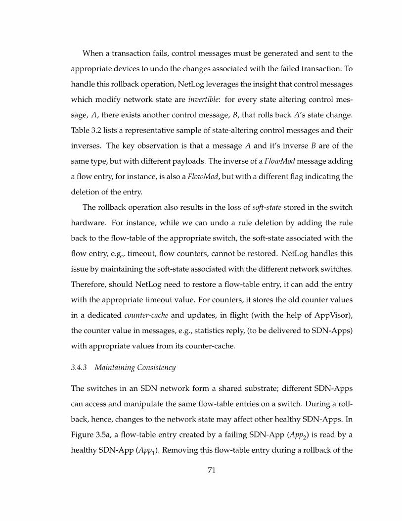
When a transaction fails, control messages must be generated and sent to the

appropriate devices to undo the changes associated with the failed transaction. To

handle this rollback operation, NetLog leverages the insight that control messages

which modify network state are invertible: for every state altering control mes-

sage, A, there exists another control message, B, that rolls back A’s state change.

Table 3.2 lists a representative sample of state-altering control messages and their

inverses. The key observation is that a message A and it’s inverse B are of the

same type, but with different payloads. The inverse of a FlowMod message adding

a flow entry, for instance, is also a FlowMod, but with a different flag indicating the

deletion of the entry.

The rollback operation also results in the loss of soft-state stored in the switch

hardware. For instance, while we can undo a rule deletion by adding the rule

back to the flow-table of the appropriate switch, the soft-state associated with the

flow entry, e.g., timeout, flow counters, cannot be restored. NetLog handles this

issue by maintaining the soft-state associated with the different network switches.

Therefore, should NetLog need to restore a flow-table entry, it can add the entry

with the appropriate timeout value. For counters, it stores the old counter values

in a dedicated counter-cache and updates, in flight (with the help of AppVisor),

the counter value in messages, e.g., statistics reply, (to be delivered to SDN-Apps)

with appropriate values from its counter-cache.

3.4.3 Maintaining Consistency

The switches in an SDN network form a shared substrate; different SDN-Apps

can access and manipulate the same flow-table entries on a switch. During a roll-

back, hence, changes to the network state may affect other healthy SDN-Apps. In

Figure 3.5a, a flow-table entry created by a failing SDN-App (App2) is read by a

healthy SDN-App (App1). Removing this flow-table entry during a rollback of the

71

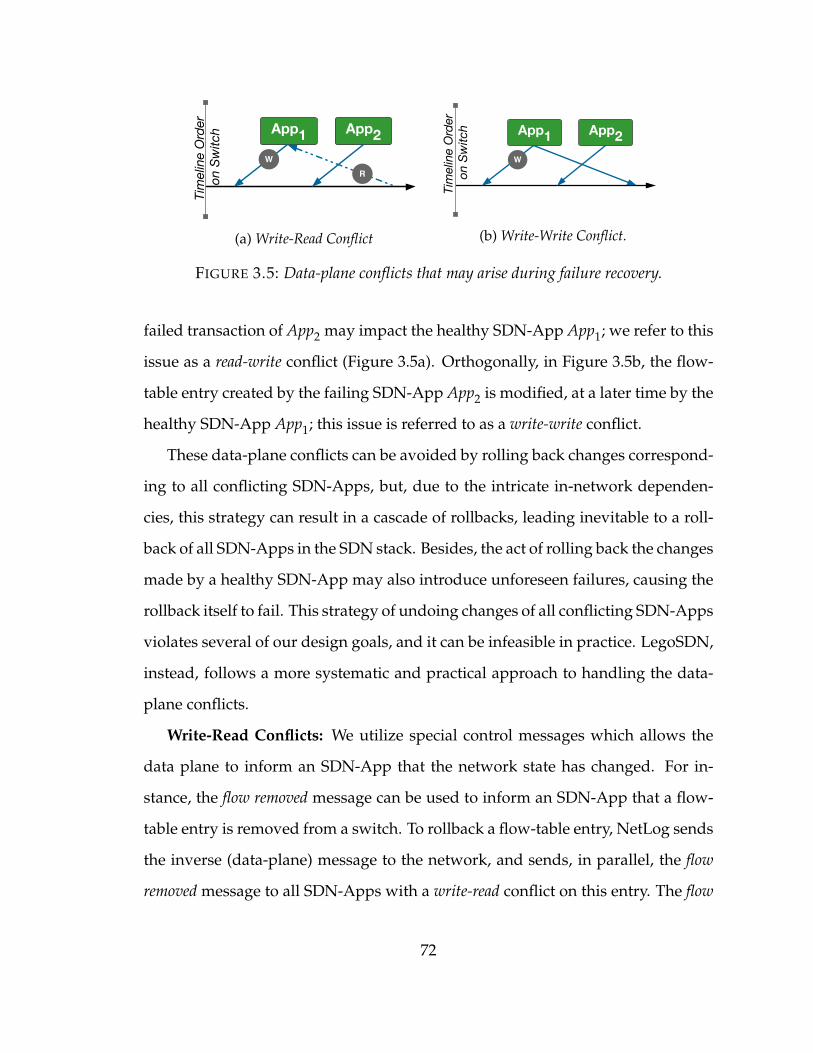
Tim

elin

e O

rder

on

Switc

h App1 App2

RW

(a) Write-Read Conflict

Tim

elin

e O

rder

on

Switc

h App1 App2W

(b) Write-Write Conflict.

FIGURE 3.5: Data-plane conflicts that may arise during failure recovery.

failed transaction of App2 may impact the healthy SDN-App App1; we refer to this

issue as a read-write conflict (Figure 3.5a). Orthogonally, in Figure 3.5b, the flow-

table entry created by the failing SDN-App App2 is modified, at a later time by the

healthy SDN-App App1; this issue is referred to as a write-write conflict.

These data-plane conflicts can be avoided by rolling back changes correspond-

ing to all conflicting SDN-Apps, but, due to the intricate in-network dependen-

cies, this strategy can result in a cascade of rollbacks, leading inevitable to a roll-

back of all SDN-Apps in the SDN stack. Besides, the act of rolling back the changes

made by a healthy SDN-App may also introduce unforeseen failures, causing the

rollback itself to fail. This strategy of undoing changes of all conflicting SDN-Apps

violates several of our design goals, and it can be infeasible in practice. LegoSDN,

instead, follows a more systematic and practical approach to handling the data-

plane conflicts.

Write-Read Conflicts: We utilize special control messages which allows the

data plane to inform an SDN-App that the network state has changed. For in-

stance, the flow removed message can be used to inform an SDN-App that a flow-

table entry is removed from a switch. To rollback a flow-table entry, NetLog sends

the inverse (data-plane) message to the network, and sends, in parallel, the flow

removed message to all SDN-Apps with a write-read conflict on this entry. The flow

72

removed notifications allow the SDN-Apps to react appropriately to the change in

the network state; the SDN-Apps are still oblivious to the rollback operation and

simply are responding to a valid network event indicating a flow-table rule re-

moval. We assume that the SDN-Apps can handle the flow-removal notification,

and this assumption will, most probably, hold since such a notification can be

generated even under normal (no failure) scenarios.

Write-Write Conflicts: In this scenario, the changes made by the failing SDN-

App have been overwritten by another SDN-App. Hence, LegoSDN neither sends

an inverse message to the network nor does it try to send messages to the healthy

SDN-Apps. Essentially, LegoSDN supports last writer wins semantics.

3.5 Event Transformations

Upon restoring the SDN-App and the data-plane to a consistent snapshot, the

SDN-App must be fed the set of inputs that it had received between the start of

the transactions and the event that caused the SDN-App to crash. The events must

be replayed to ensure that the SDN-App is aware of all changes to the network;

e.g., arrival of a new flow or a link failure.

In the best case, the replay buffer will contain one event, and in the worst-

case, it will contain N events – where N is the number of events in a cross-layer

transaction.

Traditional checkpoint-replay techniques simply replay these events in the

same order with no modifications. Unfortunately, such a strict replay of the events

only works for non-deterministic failures. In case of deterministic failures, strict

replay will result in reproducing the failure. If LegoSDN relies on such naïve re-

play mechanisms then the SDN-App will be stuck in an endless recover-replay

loop.

73

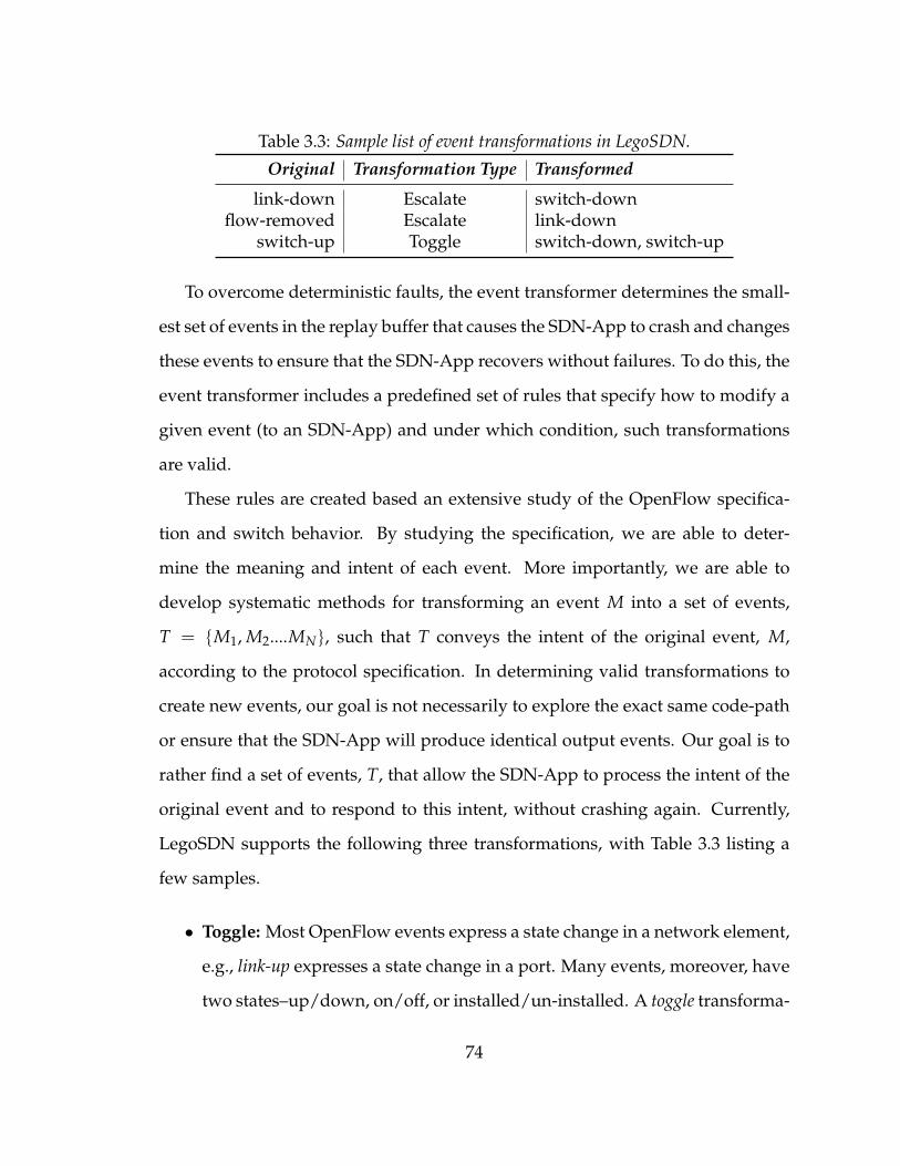
Table 3.3: Sample list of event transformations in LegoSDN.

Original Transformation Type Transformed

link-down Escalate switch-downflow-removed Escalate link-down

switch-up Toggle switch-down, switch-up

To overcome deterministic faults, the event transformer determines the small-

est set of events in the replay buffer that causes the SDN-App to crash and changes

these events to ensure that the SDN-App recovers without failures. To do this, the

event transformer includes a predefined set of rules that specify how to modify a

given event (to an SDN-App) and under which condition, such transformations

are valid.

These rules are created based an extensive study of the OpenFlow specifica-

tion and switch behavior. By studying the specification, we are able to deter-

mine the meaning and intent of each event. More importantly, we are able to

develop systematic methods for transforming an event M into a set of events,

T = tM1, M2....MNu, such that T conveys the intent of the original event, M,

according to the protocol specification. In determining valid transformations to

create new events, our goal is not necessarily to explore the exact same code-path

or ensure that the SDN-App will produce identical output events. Our goal is to

rather find a set of events, T, that allow the SDN-App to process the intent of the

original event and to respond to this intent, without crashing again. Currently,

LegoSDN supports the following three transformations, with Table 3.3 listing a

few samples.

• Toggle: Most OpenFlow events express a state change in a network element,

e.g., link-up expresses a state change in a port. Many events, moreover, have

two states–up/down, on/off, or installed/un-installed. A toggle transforma-

74

tion changes an event M into two events tM1, Mu, where M1 is the inverse of

the state represented by M. For example, a link-down is changed to tlink-up,

link-downu.

• Escalate: There is a natural hierarchy amongst network elements, e. g., a

flow table is a member of a switch, a link is a member of a switch. This

hierarchy can be leveraged in designing event transformations (Figure 3.6).

To this end, an escalate transformation changes an event M into M1, where

M1 is the equivalent state transition in the parent element. For example, a

link-down becomes a switch-down.

• Reorder: When there is more than one event in the replay buffer, a reorder

transformation can reorder the events prior to replay. When reordering

events in the replay buffer, however, LegoSDN maintains the following in-

variant: no reordering of messages from the same switch.

Restoring an SDN-App with event transformers: After restoring a crashed

SDN-App, there are two scenarios to consider during replay: the first, the last

event handled is the cause of the crash and transforming this last event, hence,

will allow the SDN-App to recover successfully; the second, the failure is the cul-

mination of one or more earlier events (essentially, not the last event). In this

work, we focus on the former and leave discussions on how to extend LegoSDN

to address the latter scenario in §3.9.

When the last event in the replay buffer is the cause of the failure, LegoSDN

replays all but the last event and transforms the last event prior to replaying it.

If replay fails, LegoSDN retries with a different transformation. This transform-

and-replay process is repeated until any of the following conditions is met: all

transformations are exhausted; (recovery) timer expired; the SDN-App success-

fully recovered from the failure.

75

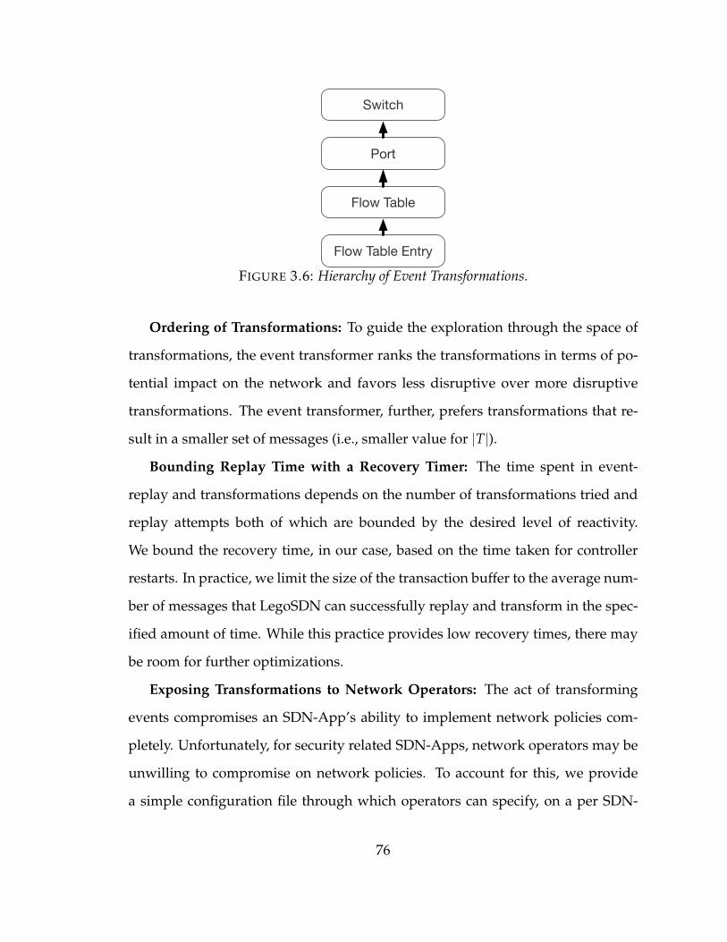
Switch

Port

Flow Table

Flow Table Entry

FIGURE 3.6: Hierarchy of Event Transformations.

Ordering of Transformations: To guide the exploration through the space of

transformations, the event transformer ranks the transformations in terms of po-

tential impact on the network and favors less disruptive over more disruptive

transformations. The event transformer, further, prefers transformations that re-

sult in a smaller set of messages (i.e., smaller value for |T|).

Bounding Replay Time with a Recovery Timer: The time spent in event-

replay and transformations depends on the number of transformations tried and

replay attempts both of which are bounded by the desired level of reactivity.

We bound the recovery time, in our case, based on the time taken for controller

restarts. In practice, we limit the size of the transaction buffer to the average num-

ber of messages that LegoSDN can successfully replay and transform in the spec-

ified amount of time. While this practice provides low recovery times, there may

be room for further optimizations.

Exposing Transformations to Network Operators: The act of transforming

events compromises an SDN-App’s ability to implement network policies com-

pletely. Unfortunately, for security related SDN-Apps, network operators may be

unwilling to compromise on network policies. To account for this, we provide

a simple configuration file through which operators can specify, on a per SDN-

76

App basis, the set of events, if any, that can be transformed and the set of valid

transformations to consider.

Ultimately, LegoSDN’s goal is to make the SDN-Apps and not the network

operators oblivious to failures. Thus, while during recovery, LegoSDN can gener-

ate a problem ticket from the captured stack-traces (or core dump), controller logs

and the offending event. This ticket can help network operators to understand

and triage the bug.

Limitations: Currently, LegoSDN supports a predefined set of transforma-

tions. The space of potential transformations, however, is larger than that cur-

rently explored. We envision that a domain-specific language will be provided to

allow developers or network operators to define new transformations.

3.6 Prototype

We developed a prototype implementation of LegoSDN6 to illustrate the utility

of our architecture. We realized our prototype by modifying the Floodlight con-

troller to include a transaction manager and an event transformer. We also made

appropriate changes to support isolation and sand-boxing of the SDN-Apps from

the controller and from each other. Although LegoSDN is designed to work with

FloodLight, the architecture and abstractions can be easily ported to other modu-

lar SDN controllers, such as, OpenDayLight [16] and ONOS [39]. Next, we discuss

the highlights of our prototype.

Sand-boxing SDN-Apps: To sandbox and isolate each SDN-App, we run each

SDN-App in a different JVM. We eliminate the need to modify or rewrite the SDN-

Apps by instrumenting the sandbox (JVM) and adding java classes to implement

the controller interface. These classes convert all local function calls from the SDN-

6 Source code of the prototype implementation and documentation is available at http://legosdn.cs.duke.edu

77

http://legosdn.cs.duke.edu

http://legosdn.cs.duke.edu

App to the controller into remote procedure calls over UDP.

At the controller, we create a proxy SDN-App that processes these remote pro-

cedure calls and converts them back into function calls to the appropriate methods

in the controller. To ensure that the SDN-Apps get all their subscribed events, the

proxy SDN-App registers itself with the controller, on behalf of the SDN-Apps, to

receive those events.

Transaction Manager: The transaction manager is implemented within the

controller as part of the proxy code that controls interactions between the SDN-

App and the controller. To create the control plane snapshots, we capture a check-

point of the SDN-App’s JVM with CRIU [71]. 7

Event-Transformer: A key property of this component is to perform consis-

tent transformations for each SDN-App. Floodlight, like most other controllers,

caches topology information within the controller and provides access to this

cache through a number of controller modules. In implementing the event-transformer,

we had to ensure that access to this cached information returned consistent trans-

formed events regardless of the controller modules used to access the cache. Since

all calls between the SDN-App and the controller happen via our proxy, we were

able to consistently enforce transformations by implementing the event-transformer

within the proxy.

3.7 Evaluation

In this section, we evaluate LegoSDN using a number of realistic SDN-Apps and

compare LegoSDN’s performance with the state-of-the-art approaches, e.g., con-

troller restarts. We quantify the time spent in various phases of recovery and

7 CRIU cannot checkpoint processes with active network connections and this posed a key chal-lenge for implementing the RPC calls between the SDN-App and the controller. This motivatedour choice of UDP as the communication channel for RPCs.

78

highlight opportunities for further improvement. We conclude by showcasing

the benefits of supporting cross-layer transactions and the capabilities of event

transformations.

3.7.1 Experimental Setup

In our experiments, we used five different SDN-Apps: Hub, Learning Switch (L.Switch),

Load Balancer (LoadBal.), Route Manager (Rt.Flow), and Stateful Firewall. These SDN-

Apps cover both the proactive and reactive development paradigms, with L.Switch,

Hub, and Stateful Firewall being reactive and the remaining being proactive SDN-

Apps. The SDN-Apps were written for the vanilla Floodlight controller and needed

no modifications to run on LegoSDN.

The SDN-Apps Hub and Learning Switch came bundled with Floodlight [42].

Hub simply floods a packet received on a switch port over all the remaining ports

on the switch. Learning Switch examines the packet to learn the MAC-address-

port mapping, flooding the packet only when a mapping is unknown. While Hub

installs no rules on any switch, Learning Switch installs rules based on the map-

pings it learns. The Route Manager SDN-App computes the shortest path dis-

tance between all pairs of hosts and pre-installs, on each switch, the route to all

reachable hosts on the network. The Load Balancer is a specialized version of

the Router Manager that attempts to evenly balance the number of flows across

different links to a given destination.

The Stateful Firewall SDN-App intercepts TCP packets between the trusted

and untrusted parts of the network and only allows the packets if the connec-

tion was initiated from the trusted part of the network; it drops any attempt to

open a connection from the untrusted part to the trusted part of the network. For

the purpose of demonstration, we designed the Stateful Firewall SDN-App not

to install any rule; hence, actual routing of the packet (once it is deemed as al-

79

lowed by Stateful Firewall) is done using Hub in our experiments. The firewall

was designed as such to make testing easier, and while the design is inefficient in

practice, it does not affect the conclusions drawn.

We used mininet [128] to emulate a network with the desired topology and

Python scripts to emulate the traffic between hosts as required for different exper-

iments. The experiments were carried out on a small testbed consisting of two

Linux servers running Ubuntu 14.04 LTS and connected by a 1 Gbps link with a

latency of 10 ms. Each machine had 12 cores with 16 GB of memory. All the ex-

periments were conducted with the controller and isolated SDN-Apps running on

one server, and with mininet and the scripts running on the other.

To crash SDN-Apps when using LegoSDN, we developed a fault-injector shim

that can be configured to generate a RuntimeException in response to a specific

input. When launching the SDN-Apps, we can pass configuration parameters

(via a properties file) to crash one or more SDN-Apps either deterministically on

a specific event, e.g., a port-down event, or randomly on any input (to emulate

non-deterministic faults). When using the SDN-Apps with the traditional Flood-

light controller, we use a carefully re-written faulty version of the SDN-Apps that

injected fault in a manner similar to that of the fault-injector shim. This fault in-

jection approach allows us to emulate most crash inducing errors except memory

corruptions.

3.7.2 Recovery Time

To compare LegoSDN against other recovery mechanisms, we crashed different

SDN-Apps, each for 60 times, by generating faults, and measured the recovery

time of each SDN-App under different recovery mechanisms. We define the re-

covery time of an SDN-App as the time between when an SDN-App (or SDN

stack) crashed and when the SDN-App was ready to process the next input. The

80

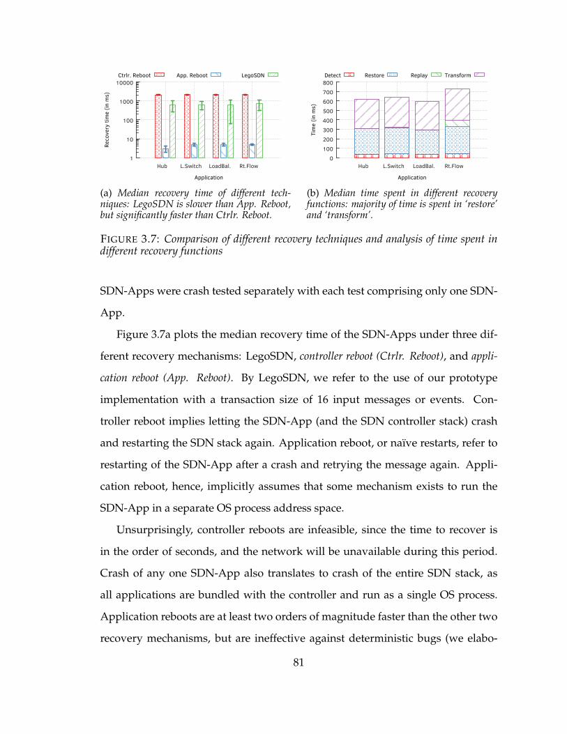
1

10

100

1000

10000

Hub L.Switch LoadBal. Rt.Flow

Reco

very

tim

e (in

ms)

Application

Ctrlr. Reboot App. Reboot LegoSDN

(a) Median recovery time of different tech-niques: LegoSDN is slower than App. Reboot,but significantly faster than Ctrlr. Reboot.

0

100

200

300

400

500

600

700

800

Hub L.Switch LoadBal. Rt.Flow

Time (in

ms)

Application

Detect Restore Replay Transform

(b) Median time spent in different recoveryfunctions: majority of time is spent in ‘restore’and ‘transform’.

FIGURE 3.7: Comparison of different recovery techniques and analysis of time spent indifferent recovery functions

SDN-Apps were crash tested separately with each test comprising only one SDN-

App.

Figure 3.7a plots the median recovery time of the SDN-Apps under three dif-

ferent recovery mechanisms: LegoSDN, controller reboot (Ctrlr. Reboot), and appli-

cation reboot (App. Reboot). By LegoSDN, we refer to the use of our prototype

implementation with a transaction size of 16 input messages or events. Con-

troller reboot implies letting the SDN-App (and the SDN controller stack) crash

and restarting the SDN stack again. Application reboot, or naïve restarts, refer to

restarting of the SDN-App after a crash and retrying the message again. Appli-

cation reboot, hence, implicitly assumes that some mechanism exists to run the

SDN-App in a separate OS process address space.

Unsurprisingly, controller reboots are infeasible, since the time to recover is

in the order of seconds, and the network will be unavailable during this period.

Crash of any one SDN-App also translates to crash of the entire SDN stack, as

all applications are bundled with the controller and run as a single OS process.

Application reboots are at least two orders of magnitude faster than the other two

recovery mechanisms, but are ineffective against deterministic bugs (we elabo-

81

rate on this point in § 3.7.3). Controller reboots, in contrast, can recover from

deterministic faults since the crash inducing message is dropped or ignored; in

fact, messages that arrive at the controller while recovery is in progress are also

dropped.

LegoSDN is slower compared to application reboots, but it is more than 3ˆ

faster than controller reboots. Similar to application reboots, the controller is not

affected and there is no loss of network control during recovery in LegoSDN. Un-

like application reboots, however, LegoSDN can recover from both non-deterministic

and deterministic faults (with support from the event transformer component).

The error bars on top of the bar plots in Figure 3.7a represent one standard de-

viation around the median recovery time. The standard deviations of recovery

times are much larger for LegoSDN compared to the rest, since some of the recov-

ery functions that LegoSDN performs, e.g., reading the checkpointed image of an

SDN-App from disk, can easily introduce a lot of variance in recovery time.

The median time spent in the different recovery functions is shown in Fig-

ure 3.7b. Majority of the recovery time is spent in restore followed by transform.

Restore refers to resurrecting the SDN-App from an earlier checkpoint and trans-

form implies converting of the crash inducing message to a different but equiv-

alent message. LegoSDN uses CRIU for checkpoint and restore operations, and

the RPC calls between the Java-based LegoSDN controller and the C-based CRIU

service introduce some overhead. LegoSDN can benefit either from performance

improvements to CRIU or from a better interface to the CRIU service. The design

of LegoSDN also makes it easier to switch to other alternatives should they prove

to be faster compared to CRIU. Time spent in replay seems only to be significant

in the case of Route Manager SDN-App, since a replay of past inputs causes the

SDN-App to recompute shortest paths which takes a considerable amount of time;

replay time is, hence, dependent on the implementation of the SDN-App.

82

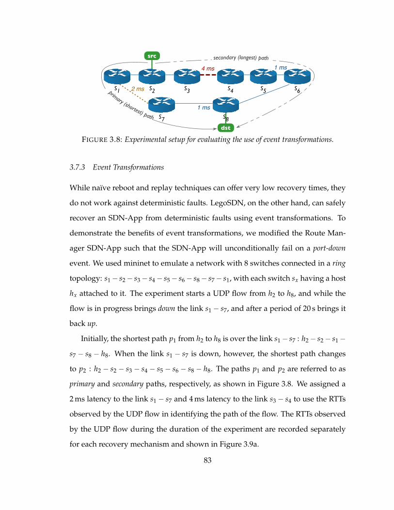
S1 S2 S3 S4 S5 S6

S7 S8

src

dst

4 ms

2 ms

1 ms

1 ms

primary (shortest) path

secondary (longest) path

FIGURE 3.8: Experimental setup for evaluating the use of event transformations.

3.7.3 Event Transformations

While naïve reboot and replay techniques can offer very low recovery times, they

do not work against deterministic faults. LegoSDN, on the other hand, can safely

recover an SDN-App from deterministic faults using event transformations. To

demonstrate the benefits of event transformations, we modified the Route Man-

ager SDN-App such that the SDN-App will unconditionally fail on a port-down

event. We used mininet to emulate a network with 8 switches connected in a ring

topology: s1´ s2´ s3´ s4´ s5´ s6´ s8´ s7´ s1, with each switch sx having a host

hx attached to it. The experiment starts a UDP flow from h2 to h8, and while the

flow is in progress brings down the link s1 ´ s7, and after a period of 20 s brings it

back up.

Initially, the shortest path p1 from h2 to h8 is over the link s1´ s7 : h2´ s2´ s1´

s7 ´ s8 ´ h8. When the link s1 ´ s7 is down, however, the shortest path changes

to p2 : h2 ´ s2 ´ s3 ´ s4 ´ s5 ´ s6 ´ s8 ´ h8. The paths p1 and p2 are referred to as

primary and secondary paths, respectively, as shown in Figure 3.8. We assigned a

2 ms latency to the link s1 ´ s7 and 4 ms latency to the link s3 ´ s4 to use the RTTs

observed by the UDP flow in identifying the path of the flow. The RTTs observed

by the UDP flow during the duration of the experiment are recorded separately

for each recovery mechanism and shown in Figure 3.9a.

83

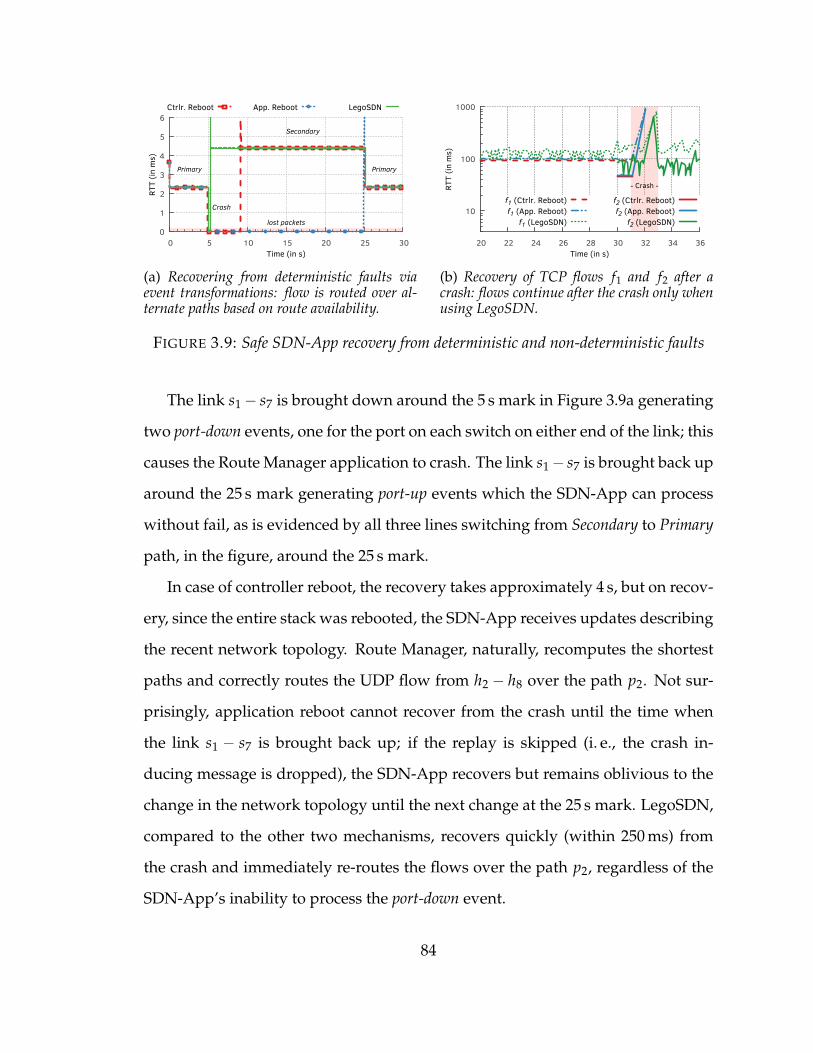
0

1

2

3

4

5

6

0 5 10 15 20 25 30

RTT (in

ms)

Time (in s)

Ctrlr. Reboot App. Reboot LegoSDN

Crash

Primary

Secondary

Primary

lost packets

(a) Recovering from deterministic faults viaevent transformations: flow is routed over al-ternate paths based on route availability.

10

100

1000

20 22 24 26 28 30 32 34 36

RTT (in

ms)

Time (in s)

f1 (Ctrlr. Reboot)f1 (App. Reboot)

f1 (LegoSDN)

f2 (Ctrlr. Reboot)f2 (App. Reboot)

f2 (LegoSDN)

- Crash -

(b) Recovery of TCP flows f1 and f2 after acrash: flows continue after the crash only whenusing LegoSDN.

FIGURE 3.9: Safe SDN-App recovery from deterministic and non-deterministic faults

The link s1´ s7 is brought down around the 5 s mark in Figure 3.9a generating

two port-down events, one for the port on each switch on either end of the link; this

causes the Route Manager application to crash. The link s1´ s7 is brought back up

around the 25 s mark generating port-up events which the SDN-App can process

without fail, as is evidenced by all three lines switching from Secondary to Primary

path, in the figure, around the 25 s mark.

In case of controller reboot, the recovery takes approximately 4 s, but on recov-

ery, since the entire stack was rebooted, the SDN-App receives updates describing

the recent network topology. Route Manager, naturally, recomputes the shortest

paths and correctly routes the UDP flow from h2 ´ h8 over the path p2. Not sur-

prisingly, application reboot cannot recover from the crash until the time when

the link s1 ´ s7 is brought back up; if the replay is skipped (i. e., the crash in-

ducing message is dropped), the SDN-App recovers but remains oblivious to the

change in the network topology until the next change at the 25 s mark. LegoSDN,

compared to the other two mechanisms, recovers quickly (within 250 ms) from

the crash and immediately re-routes the flows over the path p2, regardless of the

SDN-App’s inability to process the port-down event.

84

To recover from the deterministic fault, the event transformer transforms the

port-down events to switch-down events, effectively removing switches s1 and s7

from the topology. The event transformer, hence, presents an altered view of the

network to the SDN-App to help it recover from the fault. When the link s1 ´ s7

comes back up, it first activates the switches s1 and s7 before delivering the events

related to the new state of the link. Simply mapping messages from one to another

without maintaining a consistent per-app view of the network, will fail to re-route

the flow back to p1 at the 25 s mark.

3.7.4 Application State Recovery

Controller and application reboots are also ineffective in recovering stateful SDN-

Apps from non-deterministic failures. Using the same network topology as de-

scribed in the previous section (§ 3.7.2), but with all links set to have a latency of

1 ms, we run two SDN-Apps–Stateful Firewall and Hub–with the three recovery

mechanisms, and use two TCP flows from the trusted part to the untrusted part

of the network. The flows repeatedly open a TCP connection, send 10 packets

and close the connection. We carefully induce a fault after the TCP connection

establishment phase of one of the flows. The fault causes only Stateful Firewall

to crash, and leaves Hub intact; the experiment was setup, however, not to allow

Hub to flood without Stateful Firewall.

We measure the RTT observed from the two TCP flows– f1 and f2–and plot a

portion of the time series of RTTs in Figure 3.9b. The flow f2 (from h2 to h3) starts

30 s after the start of flow f1 (from h1 to h4). Stateful Firewall was configured

to treat hosts h1 and h2 as trusted, and hosts h3 and h4 as untrusted. The RTTs

are high since each packet is intercepted by Stateful Firewall and routed to its

destination by Hub (which floods the packet). The fluctuations in RTTs of the

flows when the SDN-Apps are deployed using LegoSDN are because of additional

85

functions, e.g., checkpointing, performed by LegoSDN. These functions, however,

are critical as the TCP flows continue after the crash only when using LegoSDN.

Without checkpointing of the SDN-Apps’ states and restoring them after the crash,

Stateful Firewall will lose the connection establishment information and hence,

will drop the TCP packets. The sender and the receiver, however, are also unaware

that they have to re-establish the connection; the sender retransmits assuming

packets are getting lost. The loss of state when recovering Stateful Firewall using

either controller or application reboot prevents the TCP flows from making any

progress after the crash (indicated by the shaded region) as shown in Figure 3.9b.

3.7.5 Cross-layer Transaction Support

We use mininet to emulate a network with 6 switches connected in a ring-like

topology: s1 ´ s2 ´ s3 ´ s4 ´ s6 ´ s5 ´ s2, with switch s1 outside the ring. Switches

s1 through s4 each have one host attached at port-1. We used a slightly modified

version of the route manager application (introduced earlier in this section) that

installs rules proactively to route flows between hosts h2 through h4 along the

path s2 ´ s3 ´ s4. Switch s5 is setup to forward all packets to s6 which in turn is

setup to forward to s4. Initially, the path through s5 and s6 remains unused and

no rules are installed on Switch s1.

Suppose that the path through s5 and s6 contains a middlebox that inspects the

traffic to check for malicious flows. After approximately 5 s, a new flow is started

from h1 to h3. Switch s1 sends the first packet to the controller which in turn

contacts the SDN-app to setup the route for the flow. The SDN-app does not trust

the flow originating from h1 and intends to route the flow over the alternate path

s1 ´ s2 ´ s5 ´ s6 ´ s4 ´ s3 (response from h3 to h1 flows over the path s3 ´ s2 ´ s1).

To this end the SDN-app installs rules on switches s4, s3, s2, s1, s6, in that order. The

SDN-app, however, is programmed to fail in the middle of this route setup—after

86

setting up s1 but before setting up s6. When NetLog is enabled changes made

to the network are reverted after a crash and, hence, the untrusted flow makes

no progress. Disabling NetLog, on the other hand, causes the untrusted flow to

proceed (over the path s1´ s2´ s3), resulting in policy violations (since the flow is

not being inspected by the middlebox on the path through s5 ´ s6).

3.8 Related Work

SDN Fault Tolerance. The most closely related works [125, 116, 118, 75] focus on

recovering from controller failures, typically, by applying Paxos [170]; there is not

much focus on handling SDN-App failures or deterministics failures, and these

faults can cripple the framework. Specifically, Ravana [118] employs a similar

notion of transactions, but, unlike LegoSDN, Ravana requires switch-side mech-

anisms and extensions to the OpenFlow interface to guarantee correctness. Rose-

mary [195], like LegoSDN, adds isolation to SDN-App. LegoSDN, however, im-

proves on Rosemary by maintaining transparency and by including a better fault

tolerance model—one that can recover from a richer set of failures.

Bugs in SDN Code. Recent work to debug SDNs focus on detecting bugs [124,

107] or debugging bugs in SDN-Apps [190, 108, 152] and SDN switches [126, 145].

Building on these existing approaches, we attack an orthogonal problem, that of

overcoming bugs which result in controller failures or violation of network invari-

ants. Our approach allows the network to guarantee availability even after bugs

trigger SDN-App failures.

Operating System Fault Tolerance. Our approach builds on several key oper-

ating system principles: isolation [50], failure oblivious computation [185], and

checkpoint-replay [117, 206]. These approaches, however, assume that bugs are

non-deterministic and thus can be fixed by a reboot [50, 117, 206]. To tackle de-

87

terministic bugs, LegoSDN extends these approaches [50, 117, 206] by employing

domain specific knowledge to transform failure inducing events into safe events.

Unlike in failure-oblivious computing [185] where transformations inject random

data, in LegoSDN transformations maintain semantic equivalence and thus en-

sure safety.

Other SDN controllers. While recent SDN controllers, e.g., Beehive [219], ONOS [39],

OpenDayLight [16], have made significant progress towards addressing controller

availability, tolerating deterministic SDN-App failures is not an objective of their

designs. LegoSDN can be easily extended to such platforms; in case of ONOS, for

instance, LegoSDN’s NetLog can be incorporated into ONOS’s global network

view.

On the other hand, approaches like Frenetic [88] and Pyretic [179] focus on

providing a better programming platform for developing SDN-Apps, thus po-

tentially eliminating bugs. The objectives of such programming platforms is to

allow developers to write modular applications with ease and such objectives are

orthogonal to that of LegoSDN. These controllers, nevertheless, neither address

isolation of SDN-App crashes nor offer support for checkpoint and recovery of

SDN-Apps. LegoSDN can, however, provide support for some of the high-level

objectives of these programming platforms, e. g., avoiding writing of redundant

or conflicting rules, by extending the AppVisor component.

3.9 Discussion

Next, we discuss several limitations of LegoSDN as well as a few interesting ap-

proaches for extending LegoSDN to address other types of failures.

Controller Failures: LegoSDN isolates the SDN-Apps from the controller and

runs them in separate processes. The approach also implies that despite the con-

88

troller crashing, an SDN-App can continue unaffected (although the SDN-App

will be unable to interact with the network).

Failures caused by Multiple Events: Although LegoSDN, currently, focuses

on failures induced by the last event processed, the system can be extended by in-

corporating STS [190] to address failures caused by an arbitrary set of events. We

envision that upon detecting a failure, LegoSDN can run STS on the failed SDN-

App to determine the minimal set of input events, S, associated with the failure.

S is then placed in the replay buffer, and LegoSDN rolls back the SDN-App to the

last checkpoint before the first message in S. The transform-and-replay process

continues from this point onwards exactly as described before. We suspect, how-

ever, that a new set of transformations may be required to improve the speed of

replay.

Network Function Virtualization (NFV) While the approaches in §3.4 focus

on network switches, we believe they can be extended to include network func-

tions. We can treat network functions like we treat switches and expand NetLog

to include network-function state by incorporating existing techniques [97] for

managing network function states. Alternatively, we could leverage existing ap-

proaches for check-pointing middleboxes [192].

Limitations of LegoSDN’s Rollback: LegoSDN’s roll back only impacts net-

work elements and not end hosts. Hence, packets sent to end hosts cannot be

modified as part of the rollback, and this leaves the end-host stack in an inconsis-

tent state. Fortunately, unlike in the SDN switches and controller, multiple layers

of failure-recovery are built into the end-host stack and the stack will adjust to the

modified network. For example, TCP contains mechanisms to deal with out of

order packets and duplicate packets.

Maintain network invariants: In case LegoSDN cannot successfully recover

from a crash (i. e., all transformations still result in a crash), LegoSDN drops the

89

input event. The SDN-App at this point can continue or be halted depending on

the SDN-App’s configuration (specified at startup). Dropping an input (message

or event) can lead to a violation of network invariants, i.e., dropping a switch-down

can result in black holes. We argue that, in general, compromising the availability

of a few flows (as a result of violating network invariants) is acceptable compared

to sacrificing control of the entire network. On the other hand, if network invari-

ants cannot ever be violated, a host of policy checkers [124] can be used to check

network invariants; in case the guarantee fails to hold, LegoSDN reverts to using

controller reboots.

3.10 Summary

Currently, SDN-Apps are used over controllers in an ad-hoc fashion, without any

isolation or abstractions to control properties for all SDN-Apps. LegoSDN demon-

strates how one can retrofit this functionality in the existing SDN stack without

any modifications to the controller or SDN-Apps. We use LegoSDN to provide

fault tolerance and address the need for a safe and fault-tolerant controller by

detecting SDN-App failures in real time and modifying network events to elim-

inate the crash. We implemented a prototype of LegoSDN based on the popular

Floodlight controller platform and show that the performance overhead of fault

tolerance is reasonable.

90

4

Alidade: Passive IP Geolocation

It’s the way I study—to understand something by trying towork it out or, in other words, to understand something by

creating it.

— Richard P. FeynmanWinner of Nobel Prize in Physics 1965

Many cloud services rely on knowing a user’s location to provide differenti-

ated services or enforce region-specific restrictions. Instead of asking each user

to provide his or her own location, which can be highly error-prone, applications

typically use one of the many commercially available geolocation packages to in-

fer a user’s location based on his or her IP address. As a result, accurate geolo-

cation is critically important to these applications. While most packages provide

accuracy guarantees, verifying these guarantees requires having access to a large

ground-truth data set that the geolocation vendors do not have access to. Perhaps

more importantly, because of the proprietary nature of commercial geolocation

packages, it is impossible to understand how they arrive at the answers that they

are providing. It is therefore difficult for a user to even reason about the accuracy

of each individual answer.

Although academic geolocation systems are not proprietary, which allows their

91

approaches to be publicly scrutinized, correctly evaluating their accuracy is still a

significant challenge. Past geolocation systems only evaluate their accuracy using

the handful of ground-truth data sets that are publicly available, such as Planet-

Lab node locations and self-reported data from friends and family. This can lead

to misleading evaluation results. For example, PlanetLab nodes, which are pri-

marily located at universities, have much more predictable latencies compared to

the average Internet end-point. This makes them far easier to locate for latency-

based geolocation systems. Furthermore, libraries such as Undns [162], which are

used by a number of academic geolocation systems, know the exact location of

most U.S. universities. They can provide inordinately accurate information for

many PlanetLab-based targets. Similarly, geolocation approaches that rely pri-

marily on external data sources, such as store front locations from Google maps,

have primarily been evaluated using favorable targets in densely populated re-

gions. Although this is likely due to a lack of available ground truth data in more

rural regions, it nevertheless underscores the difficulty in both evaluating geolo-

cation systems and making fair comparisons between them.

Not surprisingly, we find that varying the test data selection with respect to

population density and geographical coverage can dramatically affect geolocation

accuracy, as can varying the number of targets within the same IP range or the

distance between a target to its closest measurement vantage point. We also find

that many publicly available data sets fail simple speed of light-based validation,

which makes geolocation results based on them to be suspect.

This study has also led us to realize the importance of “showing your work”

when providing a geolocation answer, because knowing the intermediate steps

and the data used at each step can be helpful in debugging wildly incorrect re-

sults, in reasoning about the confidence of each individual result, and even in

determining the correctness and precision of some ground-truth data sets.

92

4.1 Contributions

Building on what we learned from evaluating geolocation systems, we developed

our own geolocation system called Alidade over the course of more than four years.

Alidade has the dual goal of being both highly accurate and completely transpar-

ent in describing how it uses its sources of information to arrive at its answers. It

is also fundamentally different from previous academic systems because it com-

putes predictions for the entire IP address space instead of for individual IP ad-

dresses, and does not issue any measurement probes of its own, either before or

after it is presented with queries. Instead, Alidade fuses available data sets of var-

ious types, attempting to resolve conflicts in the data and to find mutually com-

patible solutions for all addresses. Most importantly, unlike all other geolocation

systems, Alidade does not only return a point or area estimate as an answer, but

instead provides the exact rules and ground truth data that were used. This al-

lows a user to individually reason about the correctness of each step Alidade took

to arrive at its answer, which enables users to have confidence about an answer

without performing their own extensive tests.

At its core, Alidade is a constraint-based passive geolocation system, inspired

by Octant [217], but able to incorporate a wider variety of non-measurement data

sources. Alidade uses latency measurements only when they are issued from

hosts with known geographical locations, e.g., PlanetLab nodes. We call these

hosts and/or their IP addresses landmarks. Alidade’s estimate of the location of

an address with an unknown location, which we call a target, is represented as a

polygonal region on the surface of the Earth that should (if the prediction is correct)

contain the address. The predictions made by commercial geolocation systems, in

contrast, generally consist of a single latitude-longitude point or the name of a

city or country. To facilitate a comparison with these systems, Alidade selects a

93

single point to represent the polygon region. Although sophisticated techniques

based on population density maps could be used to pick the representative point,

at present Alidade just uses a set of heuristics that select the center of some city

contained in the answer region.

FIGURE 4.1: Example of a geolocation prediction made by Alidade for a target.

Figure 4.1 shows an example of an answer region computed by Alidade. The

region bounded by the dark green line represents the area resulting from inter-

secting constraints derived from latency measurements. In this example the inter-

section happens to be a circular region. The polygon in blue is a country-level hint

(Germany) inferred from one of the Internet registries. Since the registry data does

not conflict with the contraints derived from the measurements, Alidade uses it

to further refine its prediction. In this example, Alidade has also identified a city-

level hint (Kaiserslautern, a district in the Rhineland-Palatinate state of Germany)

by examining the names of the routers on a traceroute path to the target. The city-

level hint is indicated in the figure by the tiny red polygon inside the larger blue

one. Ultimately Alidade pins the target in this demonstration to Kaiserslautern,

which is consistent with the ground truth location of the target.

94

This chapter describes our experience in evaluating geolocation systems and

developing Alidade, which includes:

• Identifying issues in the most-commonly used data set for IP geolocation,

and how results based on this data set is unlikely to generalize the geoloca-

tion accuracy of a system across the entire IP address space.

• Highlighting issues with obtaining data sets for evaluating geolocation sys-

tems.

• Re-evaluating prior assumptions about the data source quality.

• Adapting online geolocation techniques for use in an offline geolocation sys-

tem.

• Providing a comparative evaluation of Alidade’s results with that of other

geolocation systems.

• Stressing the challenges posed by ‘hard coded’ geolocation predictions, per-

haps, used widely by commercial geolocation systems.

Our analysis of Alidade includes a breakdown of how much each type of data

aids in making accurate predictions. Not surprisingly, no single source of data

suffices to make good predictions. The data sets ingested by Alidade include la-

tency and path measurements collected for other purposes, e.g., traceroute data

from iPlane [141] and CAIDA’s Archipelago (Ark) measurement infrastructure

[47], and client-server round-trip times measured by a Content Delivery Net-

work (CDN). Alidade also relies on a tool called HostParser that translates domain

names into geographical locations, much as the Undns tool [200] does. To provide

coverage over the entire IP address space, Alidade leverages data from the Inter-

net registries too. The extent to which the registry entry for an address is trusted

95

is mitigated by the position of the corresponding Autonomous System (AS) in the

AS hierarchy produced by CAIDA [48].

To process large volumes of data, Alidade is structured as a map-reduce (Hadoop)

application. (Indeed, we started by porting Octant to Hadoop.) We conducted our

experiments using a cluster of 40 8-core servers, each with 32GB of RAM. Each

component of Alidade exhibits “embarrassing parallelism” and is implemented

as a map-reduce job. In a later section we provide a breakdown of where the Al-

idade application spends most of its time, e.g., in “preprocessing” measurement

data.

The remainder of this chapter is structured as follows. In Section 4.3, we pro-

vide a detailed overview of the related work on IP geolocation. Next, in Section 4.4

we describe the design of Alidade. In Section 4.5 we present our experimental

results, including an evaluation of the performance of Alidade, EdgeScape, and

several other commercial databases on our ground-truth data set. We conclude

the chapter with a brief discussion on future work in Section 4.6.

4.2 Acknowledgments

The chapter discusses a joint work with Mingru Bai, Michael Schoenfield, Arthur

W. Berger, Nicole Caruso, Stephen Gilliss, Bruce M. Maggs, Kyle Moses, David

Plonka, David Duff, Keung-Chi Ng, Emin Gün Sirer, Richard Weber, and Bernard

Wong.

4.3 Related Work

Past work on IP geolocation can be loosely categorized into active approaches that

perform on-demand network measurements to derive constraints on a target’s

geographic location, and passive approaches that rely only on previously collected

96

information to geolocate a target. Both approaches have advantages and disad-

vantages. Active approaches may be more accurate, but predictions may not be

available until new measurements have been taken. Passive approaches can pre-

compute predictions and hence answer queries immediately, without even requir-

ing network access at query time. Importantly, passive approaches are also unob-

trusive, and do not risk alerting or annoying the target of a prediction. But passive

approaches may not have the target-specific measurement data that would enable

better accuracy.

Alidade takes a passive geolocation approach, but Alidade does not rely ex-

clusively on coarse-grained and potentially error-prone data, such as the WHOIS

database and hostname-to-location hints. Instead, Alidade filters the hints pro-

vided by these data sets by applying constraints derived from large volumes of

passively collected network measurements.

In the following sections we examine both active and passive approaches, not-

ing where Alidade borrows techniques.

4.3.1 Active Approaches

Much of the prior work in geolocating IP addresses relies on on-demand network

measurements. IP2Geo [167] is an early IP geolocation system that introduces two

active IP geolocation techniques. The first technique is GeoPing, which requires

a deployment of landmarks of known geographic locations that can perform all-

pairs latency measurements. To predict the location a target, all landmarks probe

the target. GeoPing then selects the landmark that has the most similar latency pro-

file (the set of latency measurements from other landmarks) to the user-specified

target. It then uses the landmark’s location as the prediction for the target. Al-

though this technique is simple and easy to deploy, the location of a target cannot

be accurately predicted unless there is a landmark nearby and that landmark has

97

a similar latency profile. At present, Alidade doesn’t compile latency profiles or

compare the latency profiles of targets and landmarks. The second technique is

GeoTrack, which performs traceroutes from landmarks to the target to discover

routers on the traceroute paths whose DNS names can be interpreted geograph-

ically. From this set of routers, GeoTrack locates the target at the closest router’s

location, where distance is determined in terms of estimated network latency. Al-

idade’s “extrapolator” applies a variation of this technique. By relying only on

this relatively incomplete data source, however, GeoTrack’s geolocation accuracy

is inconsistent.

In contrast to locating the target at the closest landmark or router, Constraint-

Based Geolocation (CBG) [103] determines the location of a target by creating cir-

cles on the surface of the earth around each landmark, where each circle represents

a constraint that bounds the possible location of the target. The size of each circle

is a function of the latency between the landmark and target. CBG combines con-

straints by intersecting the circles, and selects the middle of the intersection as its

best estimate of the target’s location. One risk in taking this approach is that a sin-

gle corrupt measurement can lead to an empty intersection. At its core, Alidade is

a CBG approach.

Octant [217] builds on CBG by providing a general framework that can com-

bine both positive and negative constraints, that is, information on where the tar-

get is likely and unlikely to be, respectively. To handle uncertain or error-prone

data sources, Octant combines constraints using a weight-based mechanism that

can limit the impact of erroneous measurements. Alidade builds on the Octant

framework. In order to process large volumes of measurement data and to geolo-

cate all of the IP address space, Alidade restructures the framework into a parallel

Hadoop application so that more memory and compute cycles can be applied.

Topology-Based Geolocation (TBG) [119] uses traceroutes from the landmarks

98

to the target to discover the routers along the network paths and determine inter-

router latencies. With this data, TBG performs a global optimization to find a

physical placement of the routers and the target that minimizes inconsistencies

with the network latencies. By attempting to globally optimize the placement

of both the routers and the target, TBG is more sensitive to measurement errors,

such as inflated latencies, than constraint-based solutions, where errors tend to be

more localized. To some extent Alidade applies this approach too. In particular,

Alidade uses all available estimated latencies between pairs of addresses (land-

marks, routers, and end hosts) to jointly predict the locations of the routers and

end hosts.

Several systems [86, 220, 36, 127] have applied statistical approaches to con-

struct landmark-specific functions that map measured latencies to geographical

distances. These systems generally have significant computational requirements,

and are currently unable to make use of non-latency-based constraints. Posit [85]

presents a more recent statistical approach that, while still requiring active mea-

surements, is able to significantly reduce the required number of on-demand probes

by precomputing a statistical embedding. At present, Alidade does not construct

a sophisticated model of the relationship between latency and distance. Instead,

Alidade uniformly assumes that datagrams travel at two-thirds the speed of light,

which is very close to the speed of light in optical fiber. Hence, in converting la-

tency to distance, Alidade does not model circuitous fiber paths, nor does it model

queuing delays or any other sorts of delays. The resulting constraints tend to be

loose, but they are also hard. In particular, provided that no measurements are

corrupt and no faster-than-fiber technologies, such as microwave transmission,

are employed, the intersection of a set of constraints derived by Alidade from

direct latency measurements must contain the actual location of the target. Other

work has suggested that if latency is to be converted to distance by a simple multi-

99

plicative factor, four-ninths the speed of light might be used. The smaller constant

leads to smaller intersection areas, but these areas might be empty or might not

contain the target.

Guo et al. [104] propose mining physical addresses displayed on publicly ac-

cessible Web sites that are hosted by Web servers with IP addresses in the same

prefix as the target address, and using these physical addresses as hints to im-

prove geolocation accuracy and as sources of ground truth to support evaluations.

Caruso [53] (as part of the Alidade project) and Wang et al. [213] extend this ap-

proach by combining the mined information with latency measurements to offer

finer-grained geolocation results. Although these systems produce accurate re-

sults in certain experiments, it is difficult to ascertain their actual effectiveness in

general. First, it is tricky to determine when an organization is hosting its own

Web site. Furthermore, even when an organization does host its own site, for the

technique to work the site must list a physical address that is close to that of the

hosting location. In previous experiments the best results were obtained when

the set of geolocation targets were biased towards belonging to organizations that

typically host their own Web servers and publish physical address information on

their web pages, e.g., in one experiment reported in [213], university Web servers

hosting Web pages listing campus addresses were used as landmarks and Planet-

Lab nodes were used as targets. Nevertheless, scraped address information from

locally-hosted Web sites is a rich source of geographic data, and Alidade includes

this information as one of its many data sources.

Gill et al. [99] propose two broad classes of attacks on active measurement-

based geolocation approaches. The first misleads geolocation systems by injecting

delays to latency probes from specific landmarks at the target, thereby altering the

geolocation result by moving the centroid of the constraint intersection in a CBG-

based approach. The second targets topology-aware geolocation approaches by

100

altering inter-router latencies in traceroutes, which enables powerful adversaries

to place geolocation targets at arbitrary locations. Alidade does not attempt to

detect possible adversaries. Unlike active approaches, however, where latency

probes can often be easily identified, Alidade also uses a large body of passively

collected measurements that piggyback real user TCP connection requests and

replies. Adversaries must therefore delay legitimate TCP traffic rather than just

latency probes in order to distort much of Alidade’s input data.

There has also been considerable work on using active measurements to as-

sign artificial coordinates to Internet nodes. The latency between a pair of nodes

is then estimated by computing the distance between the two nodes in the artifi-

cial coordinate space. GNP [156] is a pioneering work in this area. GNP embeds

nodes into a low-dimensional Euclidean space, where the distance between two

nodes in the space approximates the network latency between the nodes. There

is no guarantee that the artificial coordinates map in any natural way to the true

physical locations of the nodes on the surface of the Earth, however, nor is this

a goal of GNP. Building on GNP, Vivaldi [74] introduces a decentralized network

embedding approach that obviates the need for fixed landmarks. Meridian [216]

introduces an overlay routing approach to solve network positioning problems

without needing to perform an explicit network embedding. This enables Merid-

ian to avoid intrinsic network embedding errors. Alidade (whose goal is not to

predict latencies) does not have much in common with these approaches.

4.3.2 Passive Approaches

Although active geolocation approaches can be highly accurate, their dependence

on performing on-demand network measurements make them unsuitable for many

location-aware applications. Most commercial geolocation systems, such as Max-

Mind GeoCity [143], EdgeScape [26], IPInfoDB [115], and HostIP.Info [153] have in-

101

stead adopted passive approaches, where they offer their users a pre-computed

IP-to-location database that can identify a target’s location without additional net-

work access. Unfortunately, the exact methodology for creating these databases

are generally proprietary; only the expected accuracy of these databases are typ-

ically published. However, the common understanding is that these databases

rely on a combination of domain registry information, ISP provided data, host

name hints, latency measurements, and other heuristics. Alidade relies on many

of the same sources, except that the ISP-supplied ground-truth geolocation data

(from one Tier-1 ISP) is used only for evaluation purposes and not as an input to

Alidade.

Poese et al. [174] performs an analysis of the accuracy of commericial geoloca-

tion databases. They report that while geolocation databases are extremely accu-

rate at the country level, they perform poorly at the city level. Note that Poese et

al. did not analyze EdgeScape (or Alidade).

In addition to GeoPing and GeoTrack, IP2Geo [167] also introduces GeoCluster,

a passive approach that partitions the IP address space into geographically co-

located clusters. GeoCluster then assigns each cluster to a geographic location

based on the geographic information extracted from user registration and usage

databases. The effectiveness of this approach is largely limited by the availability

of such databases, the geographic coverage of the users in the databases, and the

accuracy and freshness of the self-reported user location information. At present,

no such data is available to us, but if it were, it could be used as an input to

Alidade.

102

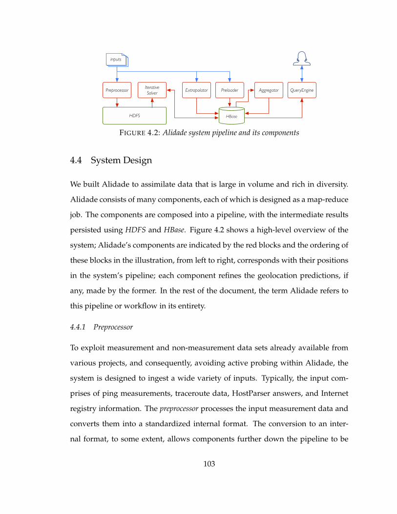
PreprocessorIterative Solver

Extrapolator Preloader Aggregator QueryEngine

inputs

HDFS HBase

FIGURE 4.2: Alidade system pipeline and its components

4.4 System Design

We built Alidade to assimilate data that is large in volume and rich in diversity.

Alidade consists of many components, each of which is designed as a map-reduce

job. The components are composed into a pipeline, with the intermediate results

persisted using HDFS and HBase. Figure 4.2 shows a high-level overview of the

system; Alidade’s components are indicated by the red blocks and the ordering of

these blocks in the illustration, from left to right, corresponds with their positions

in the system’s pipeline; each component refines the geolocation predictions, if

any, made by the former. In the rest of the document, the term Alidade refers to

this pipeline or workflow in its entirety.

4.4.1 Preprocessor

To exploit measurement and non-measurement data sets already available from

various projects, and consequently, avoiding active probing within Alidade, the

system is designed to ingest a wide variety of inputs. Typically, the input com-

prises of ping measurements, traceroute data, HostParser answers, and Internet

registry information. The preprocessor processes the input measurement data and

converts them into a standardized internal format. The conversion to an inter-

nal format, to some extent, allows components further down the pipeline to be

103

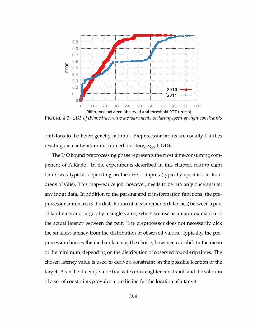
0 0.1 0.2 0.3 0.4 0.5 0.6 0.7 0.8 0.9

1

0 10 20 30 40 50 60 70 80 90 100

ECDF

Difference between observed and threshold RTT (in ms)

20102011

FIGURE 4.3: CDF of iPlane traceroute measurements violating speed-of-light constraints

oblivious to the heterogeneity in input. Preprocessor inputs are usually flat files

residing on a network or distributed file store, e.g., HDFS.

The I/O bound preprocessing phase represents the most time-consuming com-

ponent of Alidade. In the experiments described in this chapter, four-to-eight

hours was typical, depending on the size of inputs (typically specified in hun-

dreds of GBs). This map-reduce job, however, needs to be run only once against

any input data. In addition to the parsing and transformation functions, the pre-

processor summarizes the distribution of measurements (latencies) between a pair

of landmark and target, by a single value, which we use as an approximation of

the actual latency between the pair. The preprocessor does not necessarily pick

the smallest latency from the distribution of observed values. Typically, the pre-

processor chooses the median latency; the choice, however, can shift to the mean

or the minimum, depending on the distribution of observed round-trip times. The

chosen latency value is used to derive a constraint on the possible location of the

target. A smaller latency value translates into a tighter constraint, and the solution

of a set of constraints provides a prediction for the location of a target.

104

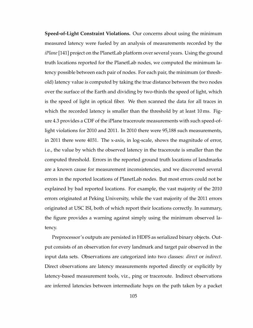
Speed-of-Light Constraint Violations. Our concerns about using the minimum

measured latency were fueled by an analysis of measurements recorded by the

iPlane [141] project on the PlanetLab platform over several years. Using the ground

truth locations reported for the PlanetLab nodes, we computed the minimum la-

tency possible between each pair of nodes. For each pair, the minimum (or thresh-

old) latency value is computed by taking the true distance between the two nodes

over the surface of the Earth and dividing by two-thirds the speed of light, which

is the speed of light in optical fiber. We then scanned the data for all traces in

which the recorded latency is smaller than the threshold by at least 10 ms. Fig-

ure 4.3 provides a CDF of the iPlane traceroute measurements with such speed-of-

light violations for 2010 and 2011. In 2010 there were 95,188 such measurements,

in 2011 there were 4031. The x-axis, in log-scale, shows the magnitude of error,

i.e., the value by which the observed latency in the traceroute is smaller than the

computed threshold. Errors in the reported ground truth locations of landmarks

are a known cause for measurement inconsistencies, and we discovered several

errors in the reported locations of PlanetLab nodes. But most errors could not be

explained by bad reported locations. For example, the vast majority of the 2010

errors originated at Peking University, while the vast majority of the 2011 errors

originated at USC ISI, both of which report their locations correctly. In summary,

the figure provides a warning against simply using the minimum observed la-

tency.

Preprocessor’s outputs are persisted in HDFS as serialized binary objects. Out-

put consists of an observation for every landmark and target pair observed in the

input data sets. Observations are categorized into two classes: direct or indirect.

Direct observations are latency measurements reported directly or explicitly by

latency-based measurement tools, viz., ping or traceroute. Indirect observations

are inferred latencies between intermediate hops on the path taken by a packet

105

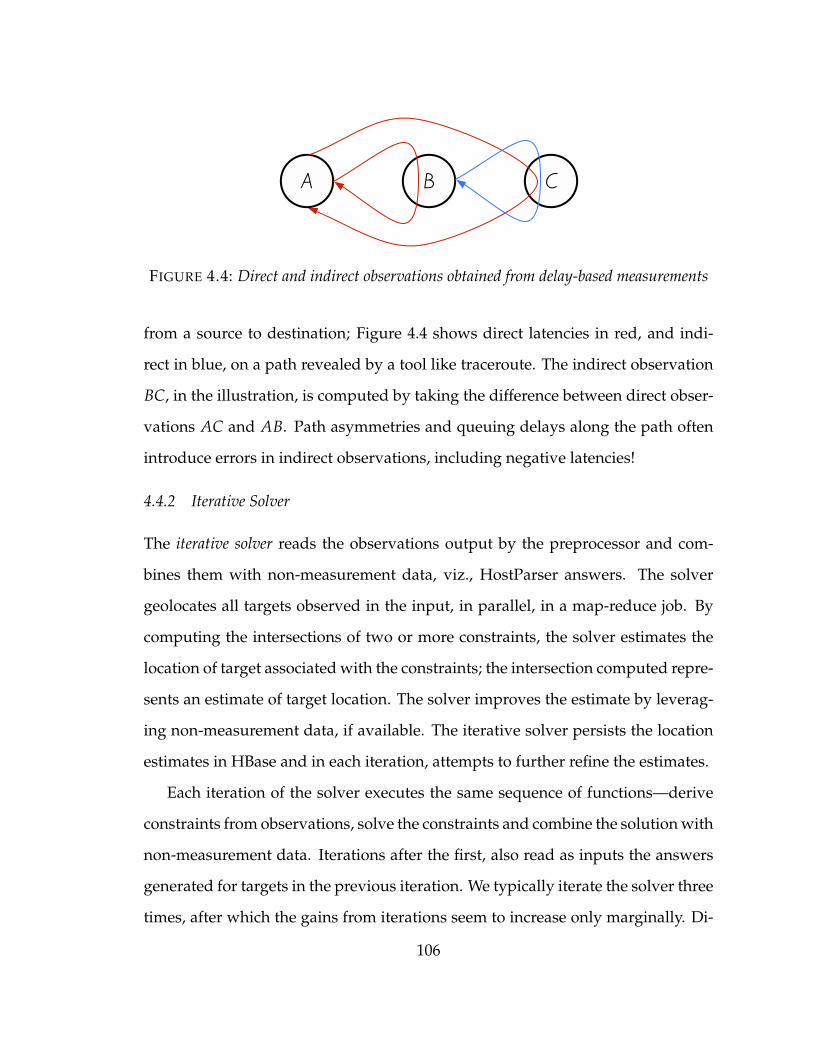
A B C

FIGURE 4.4: Direct and indirect observations obtained from delay-based measurements

from a source to destination; Figure 4.4 shows direct latencies in red, and indi-

rect in blue, on a path revealed by a tool like traceroute. The indirect observation

BC, in the illustration, is computed by taking the difference between direct obser-

vations AC and AB. Path asymmetries and queuing delays along the path often

introduce errors in indirect observations, including negative latencies!

4.4.2 Iterative Solver

The iterative solver reads the observations output by the preprocessor and com-

bines them with non-measurement data, viz., HostParser answers. The solver

geolocates all targets observed in the input, in parallel, in a map-reduce job. By

computing the intersections of two or more constraints, the solver estimates the

location of target associated with the constraints; the intersection computed repre-

sents an estimate of target location. The solver improves the estimate by leverag-

ing non-measurement data, if available. The iterative solver persists the location

estimates in HBase and in each iteration, attempts to further refine the estimates.

Each iteration of the solver executes the same sequence of functions—derive

constraints from observations, solve the constraints and combine the solution with

non-measurement data. Iterations after the first, also read as inputs the answers

generated for targets in the previous iteration. We typically iterate the solver three

times, after which the gains from iterations seem to increase only marginally. Di-

106

A B C D

estimate of location of C

(a) Use of direct constraints in IP geolocation

DA B C

dilation

estimate of location of C

(b) Use of indirect constraints in IP geolocation

FIGURE 4.5: Use of direct and indirect constraints in making a geolocation prediction fora target

rect measurement data take the highest precedence among all data sources used

in Alidade; non-measurement data that do not overlap with the direct measure-

ments are therefore discarded, without exception.

To derive constraints from latencies, Alidade multiplies them with two-thirds

the speed of light. The constraint is an N-sided polygon, with N typically set

to 32. The center of the constraint is the location of the source of the observa-

tion. Generating a constraint from a direct observation is straightforward, since

the source is a landmark; the location of a landmark is known a priori. Assume,

for instance, that a network probe takes a path from landmark A to target C via

an intermediate hop B, and another that starts at landmark D and reaches C, in

a single hop. The constraints for targets B and C using the direct measurements

from A would be polygons centered at A and sized proportional to the latencies

observed, as shown in Figure 4.5a. The illustration also shows the intersection

of two constraints, one from A and the other from D, generating a location esti-

mate for C; note that although the illustration makes use of circles for constraints,

Alidade represents them as polygons.

An indirect observation cannot be used in the first iteration, because the lo-

cation of the source of observation has not been estimated until after the first it-

107

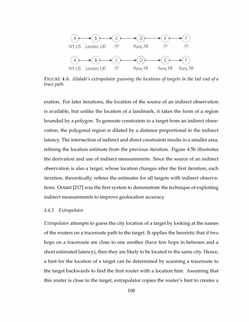
A B C D E F

NY, US London, UK ??? Paris, FR ??? ???

A B C D E F

NY, US London, UK ??? Paris, FR Paris, FR Paris, FR

FIGURE 4.6: Alidade’s extrapolator guessing the locations of targets in the tail end of atrace path

eration. For later iterations, the location of the source of an indirect observation

is available, but unlike the location of a landmark, it takes the form of a region

bounded by a polygon. To generate constraints to a target from an indirect obser-

vation, the polygonal region is dilated by a distance proportional to the indirect

latency. The intersection of indirect and direct constraints results in a smaller area,

refining the location estimate from the previous iteration. Figure 4.5b illustrates

the derivation and use of indirect measurements. Since the source of an indirect

observation is also a target, whose location changes after the first iteration, each

iteration, theoretically, refines the estimates for all targets with indirect observa-

tions. Octant [217] was the first system to demonstrate the technique of exploiting

indirect measurements to improve geolocation accuracy.

4.4.3 Extrapolator

Extrapolator attempts to guess the city location of a target by looking at the names

of the routers on a traceroute path to the target. It applies the heuristic that if two

hops on a traceroute are close to one another (have few hops in between and a

short estimated latency), then they are likely to be located in the same city. Hence,

a hint for the location of a target can be determined by scanning a traceroute to

the target backwards to find the first router with a location hint. Assuming that

this router is close to the target, extrapolator copies the router’s hint to creates a

108

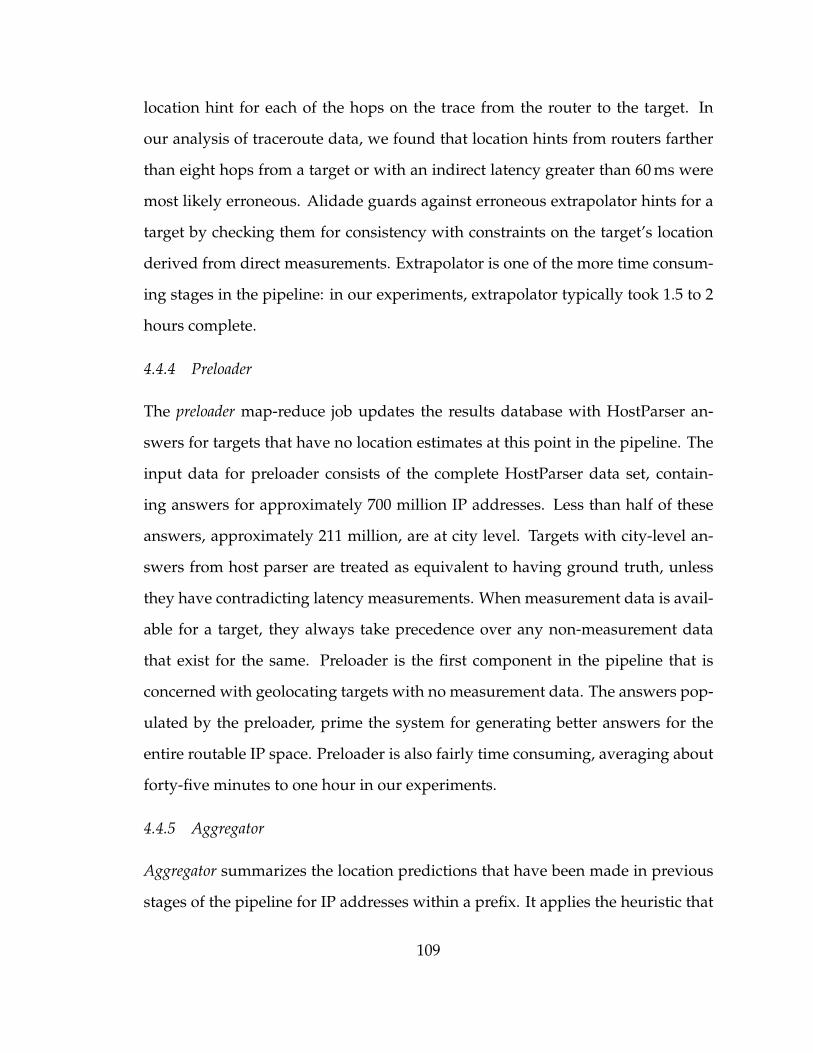
location hint for each of the hops on the trace from the router to the target. In

our analysis of traceroute data, we found that location hints from routers farther

than eight hops from a target or with an indirect latency greater than 60 ms were

most likely erroneous. Alidade guards against erroneous extrapolator hints for a

target by checking them for consistency with constraints on the target’s location

derived from direct measurements. Extrapolator is one of the more time consum-

ing stages in the pipeline: in our experiments, extrapolator typically took 1.5 to 2

hours complete.

4.4.4 Preloader

The preloader map-reduce job updates the results database with HostParser an-

swers for targets that have no location estimates at this point in the pipeline. The

input data for preloader consists of the complete HostParser data set, contain-

ing answers for approximately 700 million IP addresses. Less than half of these

answers, approximately 211 million, are at city level. Targets with city-level an-

swers from host parser are treated as equivalent to having ground truth, unless

they have contradicting latency measurements. When measurement data is avail-

able for a target, they always take precedence over any non-measurement data

that exist for the same. Preloader is the first component in the pipeline that is

concerned with geolocating targets with no measurement data. The answers pop-

ulated by the preloader, prime the system for generating better answers for the

entire routable IP space. Preloader is also fairly time consuming, averaging about

forty-five minutes to one hour in our experiments.

4.4.5 Aggregator

Aggregator summarizes the location predictions that have been made in previous

stages of the pipeline for IP addresses within a prefix. It applies the heuristic that

109

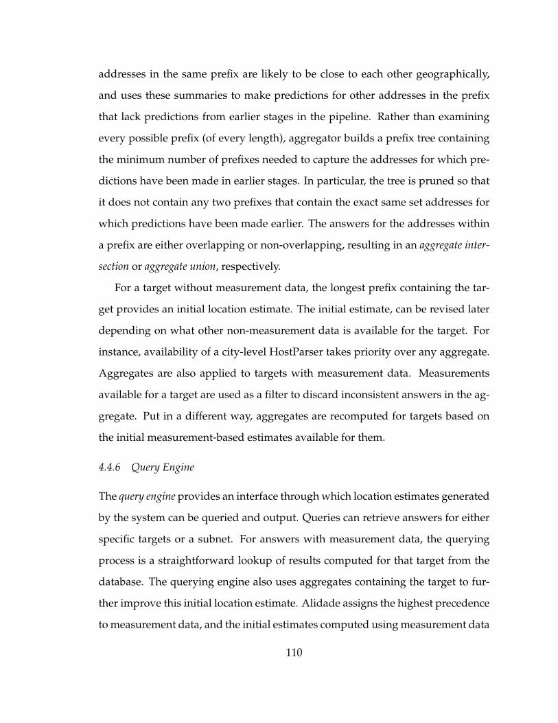
addresses in the same prefix are likely to be close to each other geographically,

and uses these summaries to make predictions for other addresses in the prefix

that lack predictions from earlier stages in the pipeline. Rather than examining

every possible prefix (of every length), aggregator builds a prefix tree containing

the minimum number of prefixes needed to capture the addresses for which pre-

dictions have been made in earlier stages. In particular, the tree is pruned so that

it does not contain any two prefixes that contain the exact same set addresses for

which predictions have been made earlier. The answers for the addresses within

a prefix are either overlapping or non-overlapping, resulting in an aggregate inter-

section or aggregate union, respectively.

For a target without measurement data, the longest prefix containing the tar-

get provides an initial location estimate. The initial estimate, can be revised later

depending on what other non-measurement data is available for the target. For

instance, availability of a city-level HostParser takes priority over any aggregate.

Aggregates are also applied to targets with measurement data. Measurements

available for a target are used as a filter to discard inconsistent answers in the ag-

gregate. Put in a different way, aggregates are recomputed for targets based on

the initial measurement-based estimates available for them.

4.4.6 Query Engine

The query engine provides an interface through which location estimates generated

by the system can be queried and output. Queries can retrieve answers for either

specific targets or a subnet. For answers with measurement data, the querying

process is a straightforward lookup of results computed for that target from the

database. The querying engine also uses aggregates containing the target to fur-

ther improve this initial location estimate. Alidade assigns the highest precedence

to measurement data, and the initial estimates computed using measurement data

110

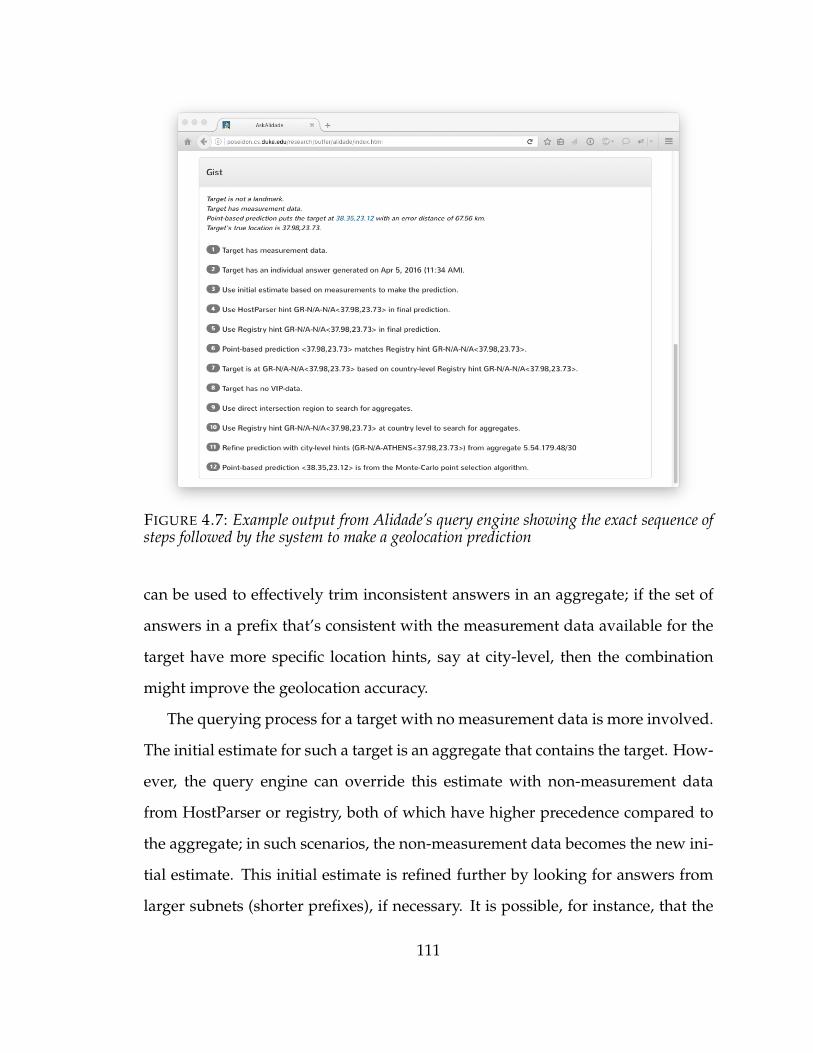
FIGURE 4.7: Example output from Alidade’s query engine showing the exact sequence ofsteps followed by the system to make a geolocation prediction

can be used to effectively trim inconsistent answers in an aggregate; if the set of

answers in a prefix that’s consistent with the measurement data available for the

target have more specific location hints, say at city-level, then the combination

might improve the geolocation accuracy.

The querying process for a target with no measurement data is more involved.

The initial estimate for such a target is an aggregate that contains the target. How-

ever, the query engine can override this estimate with non-measurement data

from HostParser or registry, both of which have higher precedence compared to

the aggregate; in such scenarios, the non-measurement data becomes the new ini-

tial estimate. This initial estimate is refined further by looking for answers from

larger subnets (shorter prefixes), if necessary. It is possible, for instance, that the

111

shortest subnet (longest prefix) used to generate the initial estimate does not have

a city-level answer. In such situations, the query engine scans for larger subnets,

provided that such aggregates contain fine-grained answers. Figure 4.7 shows an

example output from Alidade’s query engine; the figure highlights how Alidade

describes in detail the sequence of steps followed by the system to make a geolo-

cation prediction.

4.4.7 Exploiting Registry Data

Various stages in the Alidade pipeline make use of hints derived from the In-

ternet registries. One difficulty with exploiting registry data is that the operator

of a network that spans a large geographical area may list a single physical ad-

dress, which should not be trusted equally to a registry entry for a small regional

network. Alidade uses a network’s position in the Autonomous System (AS) hi-

erarchy to augment decisions to ignore a registry entry, or trust it for a country or

city-level hint.

AS hierarchy information is taken from CAIDA’s AS Ranking project [48] [140]

and is combined with Alidade’s Internet Registry data. Internet Registry entries

are mapped to BGP ASes by analyzing AS Path information from routing tables.

Consistent paths from multiple landmarks indicates a clear origin AS. Entries with

ambiguous origin are often transit networks and are generally ignored by the reg-

istry module since they have unclear localization. Alidade’s also use a network’s

prefix size for hint decisions in addition to it’s AS rank. These metrics allow us to

identify low tier and stub networks advertising small prefixes, which have con-

sistently strong [89] localization.

Internet Registry data may be checked for any IP address referenced by Ali-

dade. For a large job this could result in hundreds of millions of queries to Al-

idade’s Internet Registry datastore. Minimizing the latency of registry queries

112

can therefore have a significant impact on Alidade’s runtime. In order to max-

imize efficiency, Alidade instantiates a PATRICIA trie [146] within each reducer

task process (or JVM) in the cluster. PATRICIA tries take advantage of the hierar-

chical nature of IP address space improving latency and memory utilization. To

ensure consistency across the cluster, Registry data is delivered using Hadoop’s

Distributed Cache system.

4.4.8 Matching City Names to Shapes

A non-trivial problem encountered when exploiting data sources containing city

name hints is to convert these names into shapes. Alidade’s registry database

and HostParser table contain more than 100,000 locations (and associated coordi-

nates) from every country/region on Earth. Location names are listed as compact

ASCII strings consisting of ISO two digit country and region codes followed by

the city/location name. For example, DE-NI-OSNABRUCK is Osnabrück in the

German state of Lower Saxony (Niedersachsen). Mapping these location names

to representative shapes is conceptually simple, but nuanced in execution.

First, we compile our database from multiple open sources including postal

and census bureaus around the globe. The two primary sources are TIGER/Line

2013 (United States) [55] and GADM (worldwide) [110]. Once a source is loaded

into the database, its location names are normalized in ASCII format utilizing

Unidecode [45] to allow comparison to entries in our registry database. Conver-

sion for Latin-based languages is generally simple and error free, but translitera-

tion of non-latin languages is complex and often ambiguous. Additionally, some

location names are incredibly common, such as San Isidro, which is used to name

more than 300 locations in the Philippines. Finally, the centroids listed in the reg-

istry database inject some ambiguity since they are a limited representation of any

location (cities vary greatly in size and layout).

113

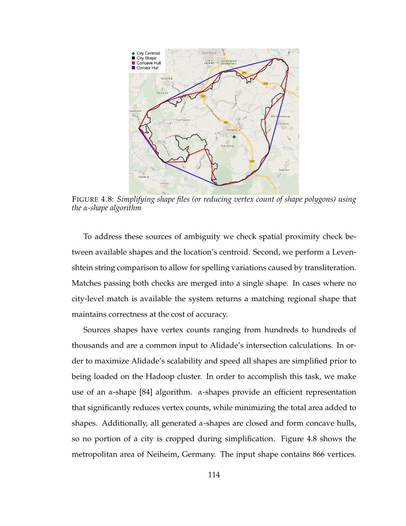
FIGURE 4.8: Simplifying shape files (or reducing vertex count of shape polygons) usingthe α-shape algorithm

To address these sources of ambiguity we check spatial proximity check be-

tween available shapes and the location’s centroid. Second, we perform a Leven-

shtein string comparison to allow for spelling variations caused by transliteration.

Matches passing both checks are merged into a single shape. In cases where no

city-level match is available the system returns a matching regional shape that

maintains correctness at the cost of accuracy.

Sources shapes have vertex counts ranging from hundreds to hundreds of

thousands and are a common input to Alidade’s intersection calculations. In or-

der to maximize Alidade’s scalability and speed all shapes are simplified prior to

being loaded on the Hadoop cluster. In order to accomplish this task, we make

use of an α-shape [84] algorithm. α-shapes provide an efficient representation

that significantly reduces vertex counts, while minimizing the total area added to

shapes. Additionally, all generated α-shapes are closed and form concave hulls,

so no portion of a city is cropped during simplification. Figure 4.8 shows the

metropolitan area of Neiheim, Germany. The input shape contains 866 vertices.

114

A simple convex hull requires only 32 vertices, but adds significant area to the

shape. In contrast, the α-shape depicted consists of only 49 vertices and retains

much of the original shape’s characteristics. Furthermore, the α parameter can be

tuned to achieve any desired tradeoff between complexity and accuracy.

4.4.9 Additional Shape Sets

We have compiled a large set of shape files for the world’s significant bodies of wa-

ter. As with city and country shapes, these water files must be simplified to allow

efficient processing. However, simply applying the same α-shape simplification

to bodies of water might expand their area, clipping adjacent land masses. This is

problematic since most population centers, and hence target locations, are often

concentrated in coastal areas. Thus, any simplification to a water shape must only

reduce its area. This can be accomplished by allowing holes in α-shape calculation

and then only retaining the interior ring of output shapes for use.

Initial testing of water shape use has revealed that they have the greatest utility

for targets with no country or city level hints, since most country and city shapes

already incorporate water boundaries. Additionally, we have discovered that a

small, but significant portion of tested location predictions from commercial com-

petitors are being placed in coastal waters and that on rare ocassion predictions

are much futher from land. Alidade’s use of alpha shapes for water areas helps

strike a balance between efficiency and accuracy in a manner unavailable to point

based geolocation systems.

4.5 Evaluation

We evaluated Alidade by comparing its answers with that of six commercial ge-

olocation databases–EdgeScape, MaxMind GeoCity, MaxMind GeoCity2 Lite, DB-IP,

IP2Location and IPligence. In this section, we begin with an exposition of the

115

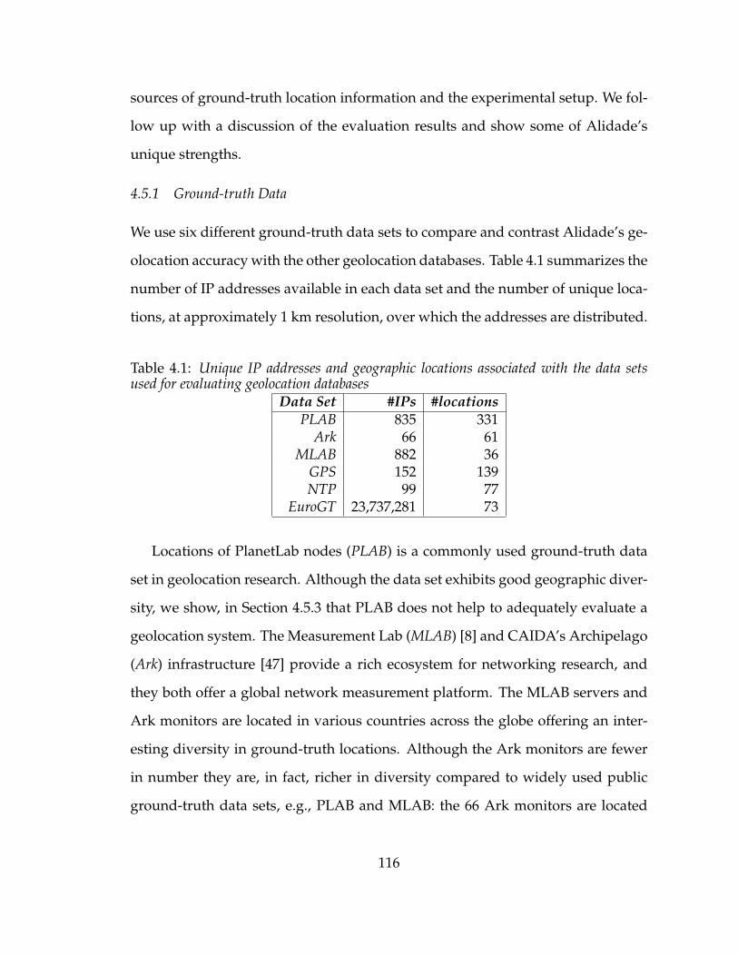
sources of ground-truth location information and the experimental setup. We fol-

low up with a discussion of the evaluation results and show some of Alidade’s

unique strengths.

4.5.1 Ground-truth Data

We use six different ground-truth data sets to compare and contrast Alidade’s ge-

olocation accuracy with the other geolocation databases. Table 4.1 summarizes the

number of IP addresses available in each data set and the number of unique loca-

tions, at approximately 1 km resolution, over which the addresses are distributed.

Table 4.1: Unique IP addresses and geographic locations associated with the data setsused for evaluating geolocation databases

Data Set #IPs #locationsPLAB 835 331

Ark 66 61MLAB 882 36

GPS 152 139NTP 99 77

EuroGT 23,737,281 73

Locations of PlanetLab nodes (PLAB) is a commonly used ground-truth data

set in geolocation research. Although the data set exhibits good geographic diver-

sity, we show, in Section 4.5.3 that PLAB does not help to adequately evaluate a

geolocation system. The Measurement Lab (MLAB) [8] and CAIDA’s Archipelago

(Ark) infrastructure [47] provide a rich ecosystem for networking research, and

they both offer a global network measurement platform. The MLAB servers and

Ark monitors are located in various countries across the globe offering an inter-

esting diversity in ground-truth locations. Although the Ark monitors are fewer

in number they are, in fact, richer in diversity compared to widely used public

ground-truth data sets, e.g., PLAB and MLAB: the 66 Ark monitors are located

116

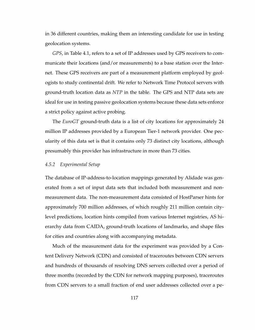
in 36 different countries, making them an interesting candidate for use in testing

geolocation systems.

GPS, in Table 4.1, refers to a set of IP addresses used by GPS receivers to com-

municate their locations (and/or measurements) to a base station over the Inter-

net. These GPS receivers are part of a measurement platform employed by geol-

ogists to study continental drift. We refer to Network Time Protocol servers with

ground-truth location data as NTP in the table. The GPS and NTP data sets are

ideal for use in testing passive geolocation systems because these data sets enforce

a strict policy against active probing.

The EuroGT ground-truth data is a list of city locations for approximately 24

million IP addresses provided by a European Tier-1 network provider. One pec-

ularity of this data set is that it contains only 73 distinct city locations, although

presumably this provider has infrastructure in more than 73 cities.

4.5.2 Experimental Setup

The database of IP-address-to-location mappings generated by Alidade was gen-

erated from a set of input data sets that included both measurement and non-

measurement data. The non-measurement data consisted of HostParser hints for

approximately 700 million addresses, of which roughly 211 million contain city-

level predictions, location hints compiled from various Internet registries, AS hi-

erarchy data from CAIDA, ground-truth locations of landmarks, and shape files

for cities and countries along with accompanying metadata.

Much of the measurement data for the experiment was provided by a Con-

tent Delivery Network (CDN) and consisted of traceroutes between CDN servers

and hundreds of thousands of resolving DNS servers collected over a period of

three months (recorded by the CDN for network mapping purposes), traceroutes

from CDN servers to a small fraction of end user addresses collected over a pe-

117

riod of three to six months, one week of ping measurements from CDN servers to

routers (recorded by the CDN to estimate network performance), and one month

of round-trip latency values recorded between CDN servers and end-user ma-

chines for a small fraction of TCP connections. The database of results created

using these measurement and non-measurement inputs was used as input to the

querying engine to geolocate the targets in the evaluation data set. The database

contains predictions for approximately 900 million targets generated using these

inputs. The selection of targets for evaluation was performed after Alidade’s

database was finalized; Alidade’s results had no influence on selection of targets

for the performance comparison.

We used the latest versions, updated in September 2013, of all the databases

except for MaxMind GeoCity, for which the last update available to us was made

in early June 2013. This is one of the reasons that we have included two databases

from the same provider in our study. MaxMind GeoLite2 City, the free version of

MaxMind, has also been widely used in academic research for evaluation of ge-

olocation systems. Alidade’s input data provided by the CDN is associated with

the third and fourth quarters of the year 2013. Our objective is to align simply the

different geolocation database systems as closer in timeline as practically possible

to ensure a fair evaluation.

Table 4.2: Number of targets in the different data sets with delay-based measurement data(for geolocation)

Data Set #targets CoveragePLAB 289 34.61%

Ark 0 0%MLAB 0 0%

GPS 12 7.89%NTP 7 7.07%

EuroGT 61,947 61.95%

118

We define error distance as the geographic distance between a system’s point-

based prediction for a target and the target’s ground-truth location. Although,

Alidade outputs polygonal regions as answers, it also computes a point-based es-

timate, which is always contained in the polygonal region. This enables a head-to-

head performance comparison of Alidade with the other geolocation databases,

all of which provide point-based predictions. Alidade uses various heuristics to

output a point-based answer. Picking the center of a city enclosed by the polygo-

nal answer, is an example of such a heuristic.

4.5.3 Comparative Evaluation Results

We begin by analyzing the effectiveness of relying solely on hints derived from the

registry or from the names of the target addresses. These are the primary sources

of non-measurement data used by Alidade. Figure 4.9b shows the ECDFs1 of er-

rors for the complete 24-million-address EuroGT dataset using only HostParser

or registry. HostParser provides answers to just a little over 20% of the targets;

for targets with no answers (approximately, 18 million) we assumed an error dis-

tance of 10,000km. Registry, by comparison, performs better, with a median error

distance of 214km. The results indicate that these two data sources alone are not

sufficient to make accurate predictions; in spite of the relatively low geographic

diversity in locations EuroGT is still a challenging data set for geolocation.

Many academic studies on geolocation have used PlanetLab nodes as the tar-

gets for evaluation, because their ground-truth locations are known (with a few

pernicious exceptions). Figure 4.9a shows that the locations of many PlanetLab

nodes can be predicted to a high degree of accuracy using information only from

the registry or from HostParser. Marginally better accuracy can be obtained by

combining these two data sets. Comparing Figures 4.9b and 4.9a, we see that the

1 Plots use log-scale for the x-axis, unless mentioned otherwise.

119

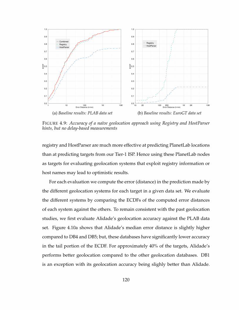
0.0

0.1

0.2

0.3

0.4

0.5

0.6

0.7

0.8

0.9

1.0

1 10 100 1K 10KError Distance (in km)

EC

DF

Combined

Registry

HostParser

(a) Baseline results: PLAB data set

0.0

0.1

0.2

0.3

0.4

0.5

0.6

0.7

0.8

0.9

1.0

10 20 100 200 1K 2K 10KError Distance (in km)

EC

DF

Registry

HostParser

(b) Baseline results: EuroGT data set

FIGURE 4.9: Accuracy of a naïve geolocation approach using Registry and HostParserhints, but no delay-based measurements

registry and HostParser are much more effective at predicting PlanetLab locations

than at predicting targets from our Tier-1 ISP. Hence using these PlanetLab nodes

as targets for evaluating geolocation systems that exploit registry information or

host names may lead to optimistic results.

For each evaluation we compute the error (distance) in the prediction made by

the different geolocation systems for each target in a given data set. We evaluate

the different systems by comparing the ECDFs of the computed error distances

of each system against the others. To remain consistent with the past geolocation

studies, we first evaluate Alidade’s geolocation accuracy against the PLAB data

set. Figure 4.10a shows that Alidade’s median error distance is slightly higher

compared to DB4 and DB5; but, these databases have significantly lower accuracy

in the tail portion of the ECDF. For approximately 40% of the targets, Alidade’s

performs better geolocation compared to the other geolocation databases. DB1

is an exception with its geolocation accuracy being slighly better than Alidade.

120

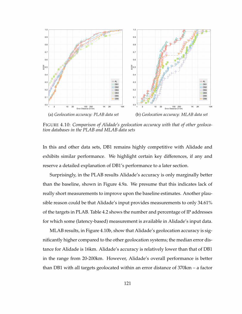
0.0

0.1

0.2

0.3

0.4

0.5

0.6

0.7

0.8

0.9

1.0

1 2 10 20 100 200 1K 2K 10KError Distance (in km)

EC

DF

AL

DB1

DB2

DB3

DB4

DB5

DB6

(a) Geolocation accuracy: PLAB data set

0.0

0.1

0.2

0.3

0.4

0.5

0.6

0.7

0.8

0.9

1.0


EC

DF

AL

DB1

DB2

DB3

DB4

DB5

DB6

(b) Geolocation accuracy: MLAB data set

FIGURE 4.10: Comparison of Alidade’s geolocation accuracy with that of other geoloca-tion databases in the PLAB and MLAB data sets

In this and other data sets, DB1 remains highly competitive with Alidade and

exhibits similar performance. We highlight certain key differences, if any and

reserve a detailed explanation of DB1’s performance to a later section.

Surprisingly, in the PLAB results Alidade’s accuracy is only marginally better

than the baseline, shown in Figure 4.9a. We presume that this indicates lack of

really short measurements to improve upon the baseline estimates. Another plau-

sible reason could be that Alidade’s input provides measurements to only 34.61%

of the targets in PLAB. Table 4.2 shows the number and percentage of IP addresses

for which some (latency-based) measurement is available in Alidade’s input data.

MLAB results, in Figure 4.10b, show that Alidade’s geolocation accuracy is sig-

nificantly higher compared to the other geolocation systems; the median error dis-

tance for Alidade is 16km. Alidade’s accuracy is relatively lower than that of DB1

in the range from 20-200km. However, Alidade’s overall performance is better

than DB1 with all targets geolocated within an error distance of 370km – a factor

121

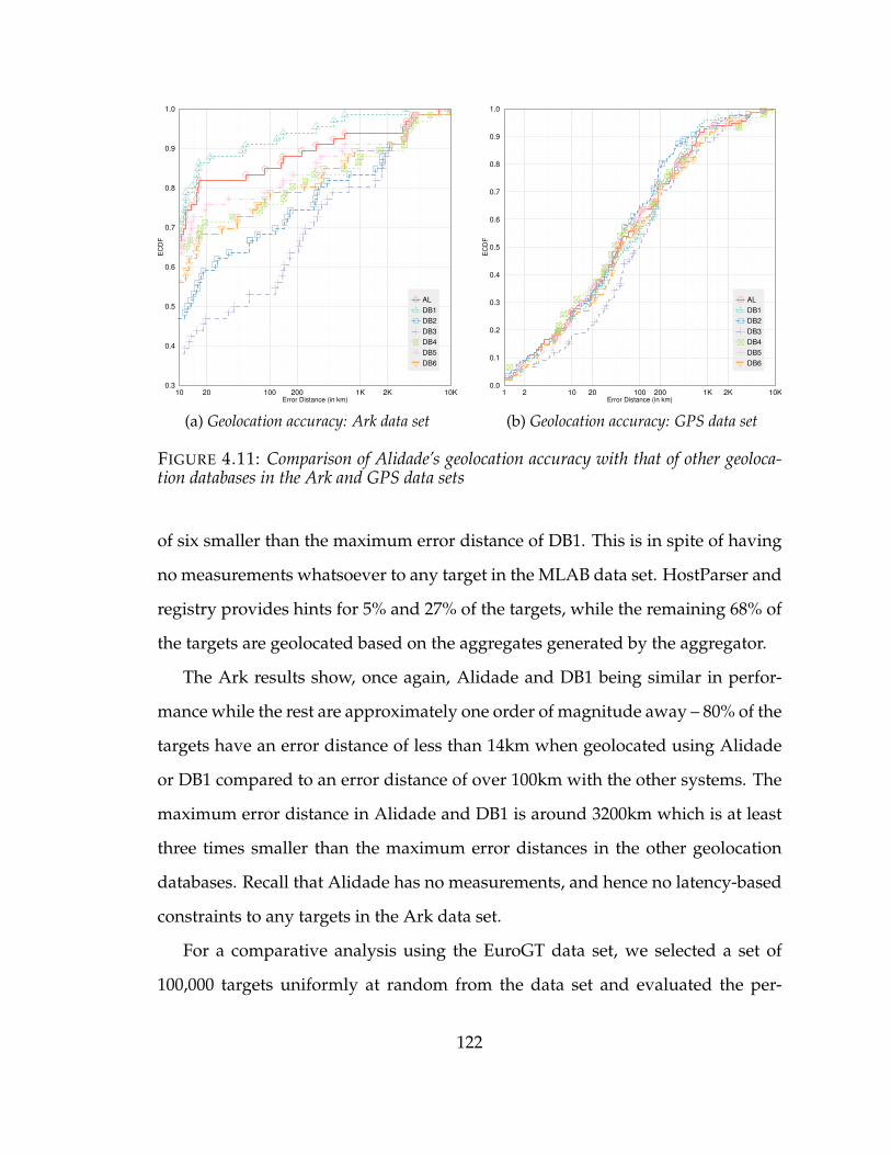
0.3

0.4

0.5

0.6

0.7

0.8

0.9

1.0

10 20 100 200 1K 2K 10KError Distance (in km)

EC

DF

AL

DB1

DB2

DB3

DB4

DB5

DB6

(a) Geolocation accuracy: Ark data set

0.0

0.1

0.2

0.3

0.4

0.5

0.6

0.7

0.8

0.9

1.0


EC

DF

AL

DB1

DB2

DB3

DB4

DB5

DB6

(b) Geolocation accuracy: GPS data set

FIGURE 4.11: Comparison of Alidade’s geolocation accuracy with that of other geoloca-tion databases in the Ark and GPS data sets

of six smaller than the maximum error distance of DB1. This is in spite of having

no measurements whatsoever to any target in the MLAB data set. HostParser and

registry provides hints for 5% and 27% of the targets, while the remaining 68% of

the targets are geolocated based on the aggregates generated by the aggregator.

The Ark results show, once again, Alidade and DB1 being similar in perfor-

mance while the rest are approximately one order of magnitude away – 80% of the

targets have an error distance of less than 14km when geolocated using Alidade

or DB1 compared to an error distance of over 100km with the other systems. The

maximum error distance in Alidade and DB1 is around 3200km which is at least

three times smaller than the maximum error distances in the other geolocation

databases. Recall that Alidade has no measurements, and hence no latency-based

constraints to any targets in the Ark data set.

For a comparative analysis using the EuroGT data set, we selected a set of

100,000 targets uniformly at random from the data set and evaluated the per-

122

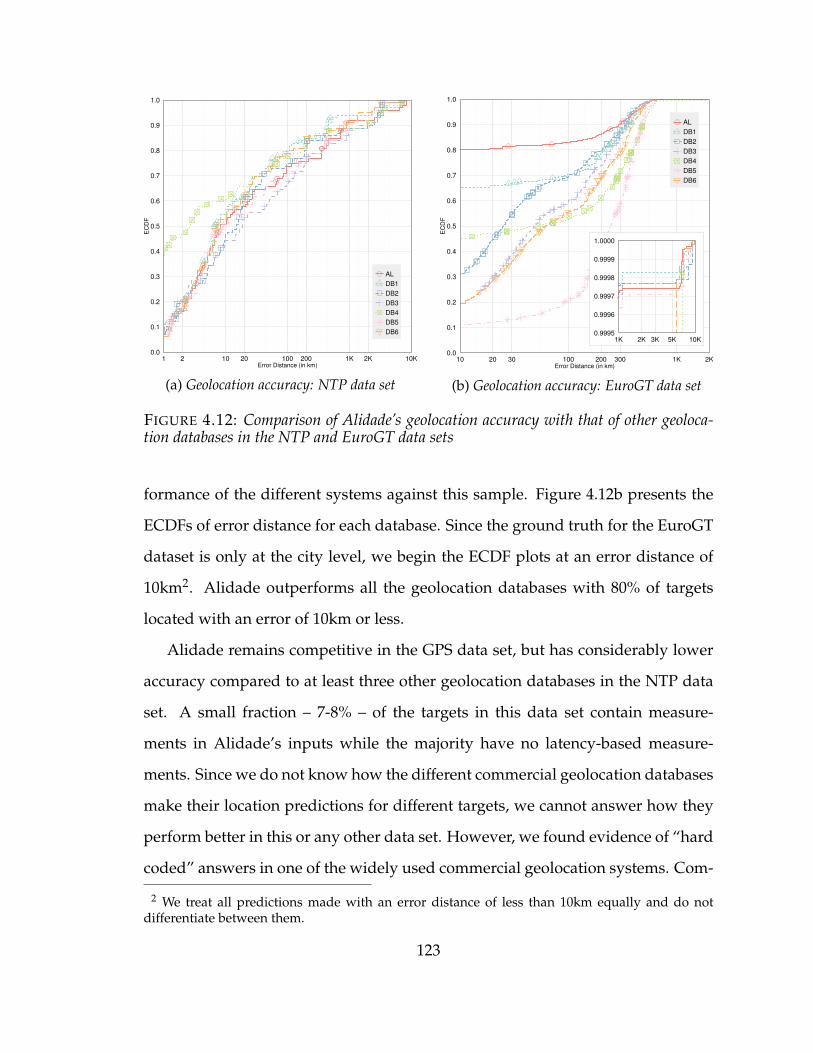
0.0

0.1

0.2

0.3

0.4

0.5

0.6

0.7

0.8

0.9

1.0


EC

DF

AL

DB1

DB2

DB3

DB4

DB5

DB6

(a) Geolocation accuracy: NTP data set

0.0

0.1

0.2

0.3

0.4

0.5

0.6

0.7

0.8

0.9

1.0

10 20 30 100 200 300 1K 2KError Distance (in km)

EC

DF

AL

DB1

DB2

DB3

DB4

DB5

DB6

0.9995

0.9996

0.9997

0.9998

0.9999

1.0000

1K 2K 3K 5K 10K

(b) Geolocation accuracy: EuroGT data set

FIGURE 4.12: Comparison of Alidade’s geolocation accuracy with that of other geoloca-tion databases in the NTP and EuroGT data sets

formance of the different systems against this sample. Figure 4.12b presents the

ECDFs of error distance for each database. Since the ground truth for the EuroGT

dataset is only at the city level, we begin the ECDF plots at an error distance of

10km2. Alidade outperforms all the geolocation databases with 80% of targets

located with an error of 10km or less.

Alidade remains competitive in the GPS data set, but has considerably lower

accuracy compared to at least three other geolocation databases in the NTP data

set. A small fraction – 7-8% – of the targets in this data set contain measure-

ments in Alidade’s inputs while the majority have no latency-based measure-

ments. Since we do not know how the different commercial geolocation databases

make their location predictions for different targets, we cannot answer how they

perform better in this or any other data set. However, we found evidence of “hard

coded” answers in one of the widely used commercial geolocation systems. Com-

2 We treat all predictions made with an error distance of less than 10km equally and do notdifferentiate between them.

123

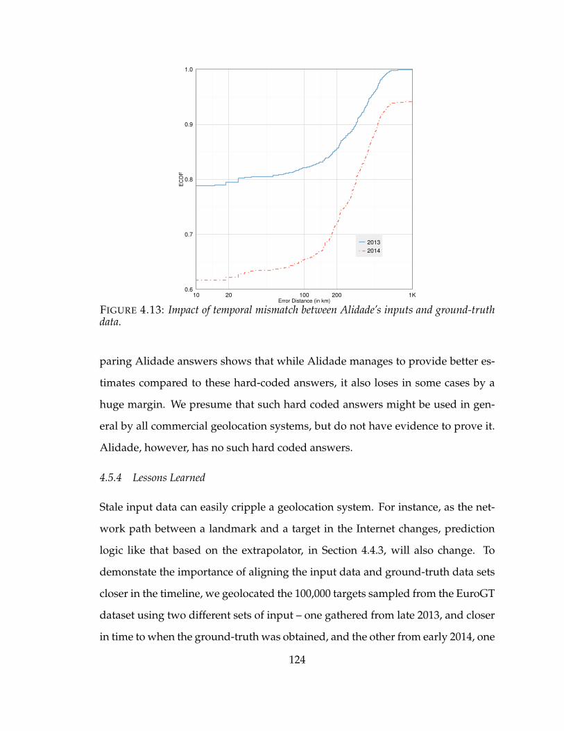
0.6

0.7

0.8

0.9

1.0

10 20 100 200 1KError Distance (in km)

EC

DF

2013

2014

FIGURE 4.13: Impact of temporal mismatch between Alidade’s inputs and ground-truthdata.

paring Alidade answers shows that while Alidade manages to provide better es-

timates compared to these hard-coded answers, it also loses in some cases by a

huge margin. We presume that such hard coded answers might be used in gen-

eral by all commercial geolocation systems, but do not have evidence to prove it.

Alidade, however, has no such hard coded answers.

4.5.4 Lessons Learned

Stale input data can easily cripple a geolocation system. For instance, as the net-

work path between a landmark and a target in the Internet changes, prediction

logic like that based on the extrapolator, in Section 4.4.3, will also change. To

demonstate the importance of aligning the input data and ground-truth data sets

closer in the timeline, we geolocated the 100,000 targets sampled from the EuroGT

dataset using two different sets of input – one gathered from late 2013, and closer

in time to when the ground-truth was obtained, and the other from early 2014, one

124

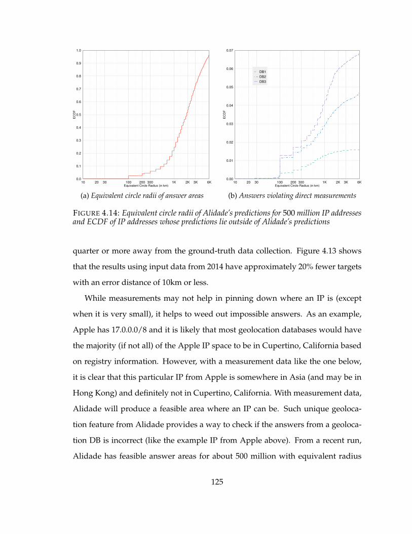
0.0

0.1

0.2

0.3

0.4

0.5

0.6

0.7

0.8

0.9

1.0

10 20 30 100 200 300 1K 2K 3K 6KEquivalent Circle Radius (in km)

EC

DF

(a) Equivalent circle radii of answer areas

0.00

0.01

0.02

0.03

0.04

0.05

0.06

0.07

10 20 30 100 200 300 1K 2K 3K 6KEquivalent Circle Radius (in km)

EC

DF

DB1

DB2

DB3

(b) Answers violating direct measurements

FIGURE 4.14: Equivalent circle radii of Alidade’s predictions for 500 million IP addressesand ECDF of IP addresses whose predictions lie outside of Alidade’s predictions

quarter or more away from the ground-truth data collection. Figure 4.13 shows

that the results using input data from 2014 have approximately 20% fewer targets

with an error distance of 10km or less.

While measurements may not help in pinning down where an IP is (except

when it is very small), it helps to weed out impossible answers. As an example,

Apple has 17.0.0.0/8 and it is likely that most geolocation databases would have

the majority (if not all) of the Apple IP space to be in Cupertino, California based

on registry information. However, with a measurement data like the one below,

it is clear that this particular IP from Apple is somewhere in Asia (and may be in

Hong Kong) and definitely not in Cupertino, California. With measurement data,

Alidade will produce a feasible area where an IP can be. Such unique geoloca-

tion feature from Alidade provides a way to check if the answers from a geoloca-

tion DB is incorrect (like the example IP from Apple above). From a recent run,

Alidade has feasible answer areas for about 500 million with equivalent radius

125

ranging from a few km to thousands of km, without observable concentration in a

particular equivalent answer radius. Using this data, we perform a check against

the answers from 3 different commercial geolocation DB and identify the ones

that the answer would be outside the Alidade feasible answer area. Figure 4.14a

shows the distribution of the answer area from this run, and Figure 4.14b shows

the results of incorrect answers from various geolocation DB. It can be observed

that we can see a non-neglible percentage of incorrect answers from all these ge-

olocation DB and a higher percentage of incorrect answers from geolocation DB

for Ips with a relatively small feasible area.

4.6 Summary

This chapter presents Alidade, a geolocation system that borrows and builds on

the best techniques from many previous systems. Unlike nearly all geolocation

systems reported in the academic literature, however, Alidade does not perform

any active probing on its own, but instead precomputes predictions for all IP ad-

dresses prior to fielding any queries. Alidade competes more directly with com-

mercial geolocation databases, and our analysis shows that Alidade is competi-

tive with a number of them on six different sets of targets for which ground-truth

physical locations are known. While we do not know the details of how the com-

peting databases are compiled, we hypothesize that Alidade makes much more

extensive use of network measurement data. Our analysis also shows that while

no one source of data suffices to provide very accurate predictions, when these

data sources are combined in the right way the overall accuracy can be quite high.

Alidade is already IPv6 compatible, but at present, we do not have much input

data related to IPv6. Geolocating mobile devices is a big challenge. Long term, we

would like to be able to identify which addresses are being used by mobile de-

126

vices and, if possible, to estimate the range of locations at which each address is

used. In determining how to combine the different inputs to make a geolocation

prediction, Alidade relies on extensive domain knowledge, encoded in a vari-

ety of heuristics. A more systematic and pragmatic approach would be to use a

machine-learning algorithm, e.g., decision tree learning, to explore the heuristics-

space and design better heuristics for improving the accuracy of predictions.

The existence of various network measurement data sets in the public do-

main, and, in particular, in a cloud ecosystem present nice incentives to build

non-intrusive passive geolocation systems. Alidade highlights the feasibility of

such an approach.

127

5

The Internet at the Speed of Light

The speed of light sucks.

— John D. CarmackCreator of Wolfenstein 3D, Quake and Doom

Reducing latency across the Internet is of immense value—measurements and

analysis by Internet giants have shown that shaving a few hundred milliseconds

from the time for a transaction can translate into millions of dollars. For Ama-

zon, a 100 ms latency penalty implies a 1% sales loss [133]; for Google, an addi-

tional delay of 400 ms in search responses reduces search volume by 0.74%; and

for Bing, 500 ms of latency decreases revenue per user by 1.2% [44, 189]. Under-

cutting a competitor’s latency by as little as 250 ms is considered a competitive

advantage [135] in the industry. Even more crucially, these numbers underscore

that latency is a key determinant of user experience and, in a cloud-computing

model, is vital to monetizing cloud services.

While latency reductions of a few hundred milliseconds are valuable, we take

the position that the networking community should pursue a much more ambi-

tious goal: cutting Internet latencies to close to the limiting physical constraint, the

128

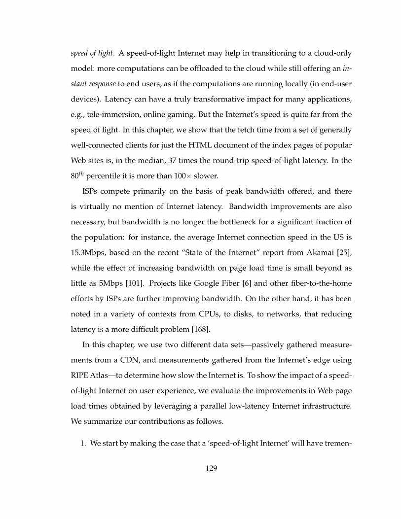
speed of light. A speed-of-light Internet may help in transitioning to a cloud-only

model: more computations can be offloaded to the cloud while still offering an in-

stant response to end users, as if the computations are running locally (in end-user

devices). Latency can have a truly transformative impact for many applications,

e.g., tele-immersion, online gaming. But the Internet’s speed is quite far from the

speed of light. In this chapter, we show that the fetch time from a set of generally

well-connected clients for just the HTML document of the index pages of popular

Web sites is, in the median, 37 times the round-trip speed-of-light latency. In the

80th percentile it is more than 100ˆ slower.

ISPs compete primarily on the basis of peak bandwidth offered, and there

is virtually no mention of Internet latency. Bandwidth improvements are also

necessary, but bandwidth is no longer the bottleneck for a significant fraction of

the population: for instance, the average Internet connection speed in the US is

15.3Mbps, based on the recent “State of the Internet” report from Akamai [25],

while the effect of increasing bandwidth on page load time is small beyond as

little as 5Mbps [101]. Projects like Google Fiber [6] and other fiber-to-the-home

efforts by ISPs are further improving bandwidth. On the other hand, it has been

noted in a variety of contexts from CPUs, to disks, to networks, that reducing

latency is a more difficult problem [168].

In this chapter, we use two different data sets—passively gathered measure-

ments from a CDN, and measurements gathered from the Internet’s edge using

RIPE Atlas—to determine how slow the Internet is. To show the impact of a speed-

of-light Internet on user experience, we evaluate the improvements in Web page

load times obtained by leveraging a parallel low-latency Internet infrastructure.

We summarize our contributions as follows.

1. We start by making the case that a ‘speed-of-light Internet’ will have tremen-

129

dous impact on cloud computing.

2. We quantify the latency in Internet using two measurement data sets: be-

tween a large CDN provider’s servers and end hosts; and between RIPE

Atlas nodes.

3. In experiments across 108 Web pages using a record-and-replay tool, we

found that eliminating infrastructural latency could cut Web page load times

by 30%.

5.1 Acknowledgments

The work presented in this chapter is the result of a joint effort with Ankit Singla,

Brighten Godfrey and Bruce Maggs. We proposed a idea of a Speed-of-Light Inter-

net in “The Internet at the Speed of Light” [196] and followed it with a manuscript,

“Towards a Speed of Light Internet” [197], which included a design sketch of a

parallel low-latency infrastructure and experiments to demonstrate the impact of

this parallel infrastructure on user experience.

5.2 The Need for Speed

A speed-of-light Internet would enhance user satisfaction with Web applications,

as well as voice and video communication. The gaming industry, where lower

latencies are crucial for an interactive gameplay, would also enjoy immense bene-

fits. Indeed, a speed-of-light Internet would be fundamentally alter the computing

landscape.

Cloud Computing. One of the biggest advantages of a speedier Internet is further

centralization of compute resources. People are already using Web-based software

for carrying out tasks that were previously done using software running locally on

130

their own devices. Google and VMware are already jointly working towards the

thin client model through virtualization [90]. Products like the Chromebook [1],

a laptop with almost all of the software powered by cloud-based services, also

highlight the shift to a cloud-computing (or thin-client) model. This shift to a

(logically centralized) cloud computing model, however, is limited by Internet’s

latency; extending the model, in particular, to end users encounters the all-too-

well-known latency issues of the last mile [102].

The increasing adoption of mobile devices with limited processing power and

resources also catalyzes the shift to a cloud-computing model. There is interest,

for instance, in offloading computations to the cloud to save energy and also to

leverage data and computational resources of the cloud, which are unavailable on

user devices [72]. Applications such as Apple’s Siri [159] and Google Now [78]

already offload some processing from their respective mobile platforms to the

cloud. The performance of these applications highly depend on having low re-

sponse times; the level of interactivity required for such applications, otherwise,

become impractical to implement. As prior work [105] has argued, however, to

achieve highly responsive performance from cloud-based applications would to-

day require the presence of a large number of data center facilities. With a speed-

ier Internet, the ‘thin client’ model becomes plausible for both desktop and mobile

computing with far fewer installations. Latency, essentially, dictates the feasibility

and even monetization of cloud services.

Better Geolocation. A speed-of-light Internet may also enable accurate geolo-

cation. Consider, for example, a client located a certain distance away from a

server. Over a speed-of-light Internet, the round-trip latency will reveal to the

server precisely this distance (assuming that other delays, e.g., server processing

delay, queueing delay are negligible). Simple constraint-based techniques, e.g.,

131

triangulation of measurements from multiple locations, may yield highly accu-

rate geolocation over a speed-of-light Internet. While better geolocation provides

benefits such as better targeting of services and matching with nearby servers, it

also has other implications, such as for privacy.

New Applications. A Speed-of-Light Interest will help in creating a convincing

experience of joining two distant locations. Applications like tele-immersion and

remote collaborative music performance are hampered today by poor Internet la-

tencies. For instance, latencies above 50ms, make remote collaboration on music

difficult [67]. Convincing virtual reality immersion necessitates a latency of less

than 20ms [223], and a similar limit likely applies to immersion in remote, real-

world environments. A Speed-of-Light Internet may help in realizing many (as of

yet unknown and unexplored) innovative applications—the latency limitations

might indeed be the only impediment for designers to think about such latency-

sensitive but “killer” applications.

CDNs and a faster Internet. CDNs reduce latency by placing a large number

of replicas of content across the globe, so that for most customers, some replica

is nearby. This approach, however, has its limitations. First, CDNs are not rel-

evant for all communication types: some resources simply cannot be replicated

or moved, such as people. Second, CDNs today are an expensive option, avail-

able only to larger Internet companies. A speedier Internet would significantly

cut costs for CDNs, putting them within reach of a larger spectrum of Web ser-

vice providers. CDNs make a trade-off between costs (determined, in part, by the

number of infrastructure locations), and latency targets. For any latency target

a CDN desires to achieve globally, given the Internet’s communication latency,

a certain minimum number of locations are required. Speeding up the Internet

improves this entire trade-off curve.

132

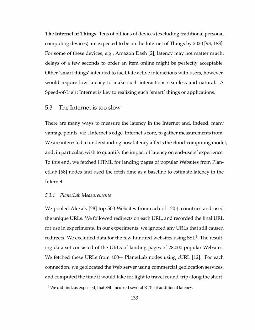
The Internet of Things. Tens of billions of devices (excluding traditional personal

computing devices) are expected to be on the Internet of Things by 2020 [93, 183].

For some of these devices, e.g., Amazon Dash [2], latency may not matter much;

delays of a few seconds to order an item online might be perfectly acceptable.

Other ‘smart things’ intended to facilitate active interactions with users, however,

would require low latency to make such interactions seamless and natural. A

Speed-of-Light Internet is key to realizing such ‘smart’ things or applications.

5.3 The Internet is too slow

There are many ways to measure the latency in the Internet and, indeed, many

vantage points, viz., Internet’s edge, Internet’s core, to gather measurements from.

We are interested in understanding how latency affects the cloud-computing model,

and, in particular, wish to quantify the impact of latency on end-users’ experience.

To this end, we fetched HTML for landing pages of popular Websites from Plan-

etLab [68] nodes and used the fetch time as a baseline to estimate latency in the

Internet.

5.3.1 PlanetLab Measurements

We pooled Alexa’s [28] top 500 Websites from each of 120+ countries and used

the unique URLs. We followed redirects on each URL, and recorded the final URL

for use in experiments. In our experiments, we ignored any URLs that still caused

redirects. We excluded data for the few hundred websites using SSL1. The result-

ing data set consisted of the URLs of landing pages of 28,000 popular Websites.

We fetched these URLs from 400+ PlanetLab nodes using cURL [12]. For each

connection, we geolocated the Web server using commercial geolocation services,

and computed the time it would take for light to travel round-trip along the short-

1 We did find, as expected, that SSL incurred several RTTs of additional latency.

133

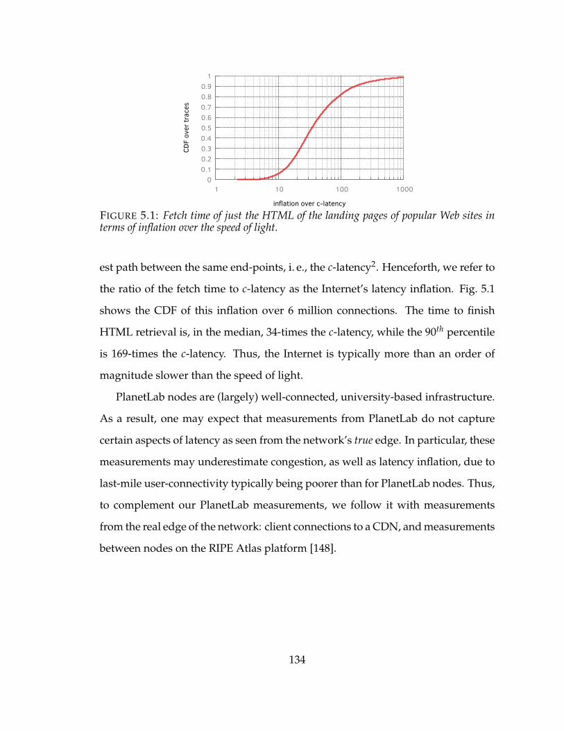
0 0.1 0.2 0.3 0.4 0.5 0.6 0.7 0.8 0.9

1

1 10 100 1000CD

F ov

er trac

es

inflation over c-latency

FIGURE 5.1: Fetch time of just the HTML of the landing pages of popular Web sites interms of inflation over the speed of light.

est path between the same end-points, i. e., the c-latency2. Henceforth, we refer to

the ratio of the fetch time to c-latency as the Internet’s latency inflation. Fig. 5.1

shows the CDF of this inflation over 6 million connections. The time to finish

HTML retrieval is, in the median, 34-times the c-latency, while the 90th percentile

is 169-times the c-latency. Thus, the Internet is typically more than an order of

magnitude slower than the speed of light.

PlanetLab nodes are (largely) well-connected, university-based infrastructure.

As a result, one may expect that measurements from PlanetLab do not capture

certain aspects of latency as seen from the network’s true edge. In particular, these

measurements may underestimate congestion, as well as latency inflation, due to

last-mile user-connectivity typically being poorer than for PlanetLab nodes. Thus,

to complement our PlanetLab measurements, we follow it with measurements

from the real edge of the network: client connections to a CDN, and measurements

between nodes on the RIPE Atlas platform [148].

134

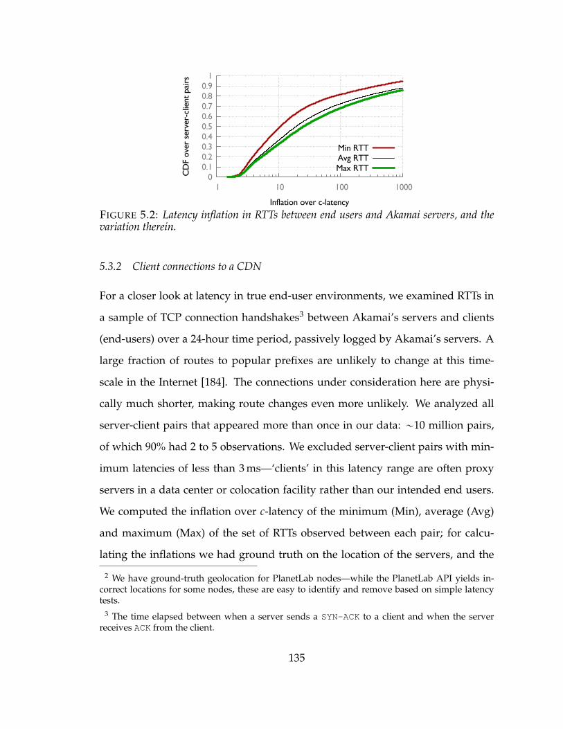
0 0.1 0.2 0.3 0.4 0.5 0.6 0.7 0.8 0.9

1

1 10 100 1000C

DF

over

ser

ver-

clie

nt p

airs

Inflation over c-latency

Min RTTAvg RTTMax RTT

FIGURE 5.2: Latency inflation in RTTs between end users and Akamai servers, and thevariation therein.

5.3.2 Client connections to a CDN

For a closer look at latency in true end-user environments, we examined RTTs in

a sample of TCP connection handshakes3 between Akamai’s servers and clients

(end-users) over a 24-hour time period, passively logged by Akamai’s servers. A

large fraction of routes to popular prefixes are unlikely to change at this time-

scale in the Internet [184]. The connections under consideration here are physi-

cally much shorter, making route changes even more unlikely. We analyzed all

server-client pairs that appeared more than once in our data: „10 million pairs,

of which 90% had 2 to 5 observations. We excluded server-client pairs with min-

imum latencies of less than 3 ms—‘clients’ in this latency range are often proxy

servers in a data center or colocation facility rather than our intended end users.

We computed the inflation over c-latency of the minimum (Min), average (Avg)

and maximum (Max) of the set of RTTs observed between each pair; for calcu-

lating the inflations we had ground truth on the location of the servers, and the

2 We have ground-truth geolocation for PlanetLab nodes—while the PlanetLab API yields in-correct locations for some nodes, these are easy to identify and remove based on simple latencytests.

3 The time elapsed between when a server sends a SYN-ACK to a client and when the serverreceives ACK from the client.

135

5

10

15

20

25

30

35

40

00-1:59 4-5:59 8-9:59 12-13:59 16-17:59 20-21:59

Med

ian

RTT

(in

ms)

Time (in UTC)

US (CST)US (EST)

GBDE

JP

(a) Medians of RTTs of client-server pairs withmeasurements in each 2-hr window

0

20

40

60

80

100

120

140

00-1:59 4-5:59 8-9:59 12-13:59 16-17:59 20-21:59

90th

per

cent

ile R

TT (

in m

s)

Time (in UTC)

US (CST)US (EST)

GBDE

JP

(b) 90th percentiles of RTTs the same set ofclient-set pairs

FIGURE 5.3: Variations in latencies of client-server pairs grouped into 2-hr windows indifferent geographic regions

clients were geolocated using data from Akamai EdgeScape [26].

To evaluate the impact of congestion, we examine our data for both variations

across time-of-day (perhaps latencies are, as a whole, significantly larger in peak

traffic hours), and within short periods of time for the same server-client pairs

(perhaps transient congestion for individual connections is a significant problem).

Thus, we discard server-client pairs that do not have repeat measurements. For

ease of analysis over time-of-day, we only look at pairs within the same country.

We include here results for a few geographies that have a large number of mea-

surements after these restrictions. We bin all RTT measurements into 12 2-hour

periods and produce results aggregated over these bins separately for each coun-

try.

Time-of-day latency variations across bins. We selected server-client pairs that

have at least one RTT measurement in each of the twelve bins. For pairs with

multiple RTTs within a bin, we use the median RTT as representative, discarding

other measurements. This leaves us with the same number of samples between

the same host-pairs in all bins. Fig. 5.3a and Fig. 5.3b show the median and the 90th

percentile of RTTs in each 2-hour bin for each of 5 timezones. For the United States

136

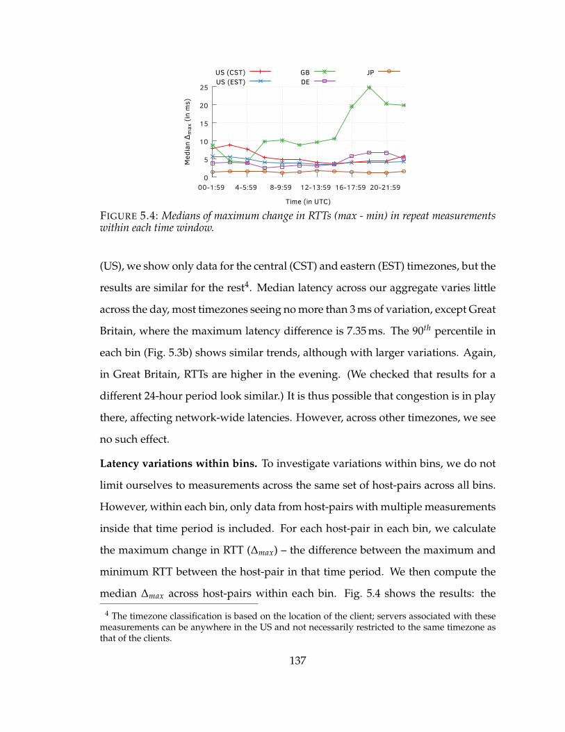
0

5

10

15

20

25

00-1:59 4-5:59 8-9:59 12-13:59 16-17:59 20-21:59M

edia

n Δ

max

(in

ms)

Time (in UTC)

US (CST)US (EST)

GBDE

JP

FIGURE 5.4: Medians of maximum change in RTTs (max - min) in repeat measurementswithin each time window.

(US), we show only data for the central (CST) and eastern (EST) timezones, but the

results are similar for the rest4. Median latency across our aggregate varies little

across the day, most timezones seeing no more than 3 ms of variation, except Great

Britain, where the maximum latency difference is 7.35 ms. The 90th percentile in

each bin (Fig. 5.3b) shows similar trends, although with larger variations. Again,

in Great Britain, RTTs are higher in the evening. (We checked that results for a

different 24-hour period look similar.) It is thus possible that congestion is in play

there, affecting network-wide latencies. However, across other timezones, we see

no such effect.

Latency variations within bins. To investigate variations within bins, we do not

limit ourselves to measurements across the same set of host-pairs across all bins.

However, within each bin, only data from host-pairs with multiple measurements

inside that time period is included. For each host-pair in each bin, we calculate

the maximum change in RTT (∆max) – the difference between the maximum and

minimum RTT between the host-pair in that time period. We then compute the

median ∆max across host-pairs within each bin. Fig. 5.4 shows the results: the

4 The timezone classification is based on the location of the client; servers associated with thesemeasurements can be anywhere in the US and not necessarily restricted to the same timezone asthat of the clients.

137

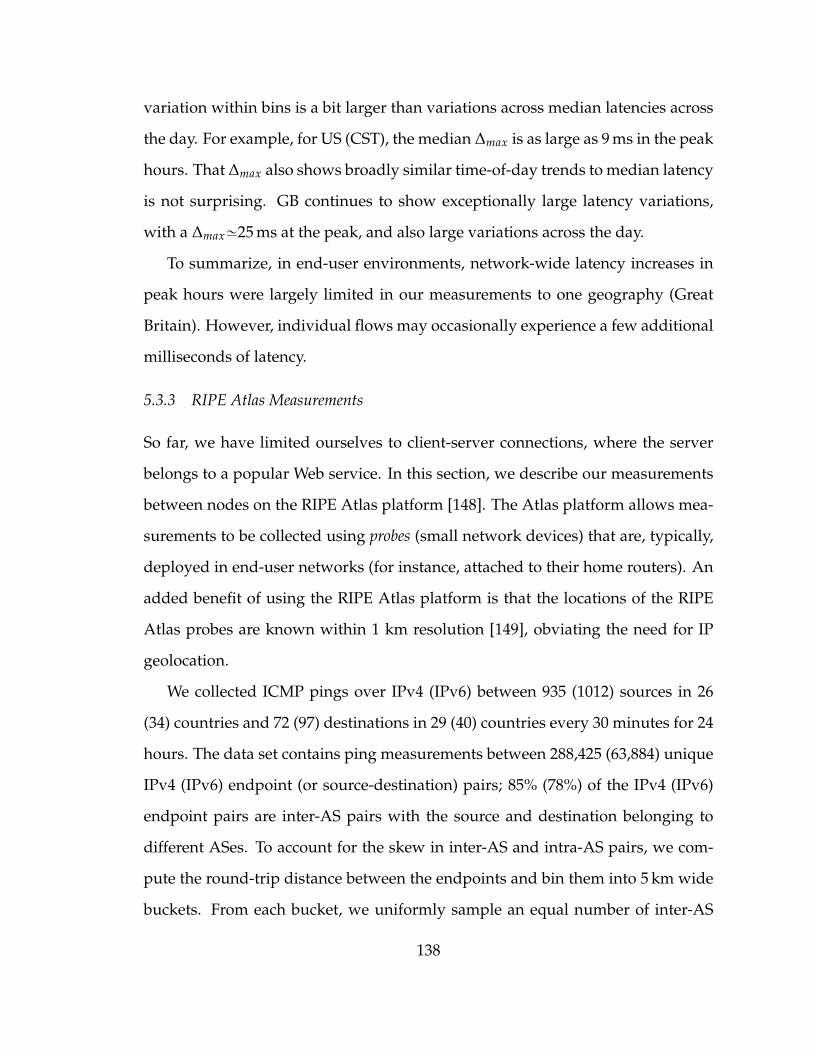
variation within bins is a bit larger than variations across median latencies across

the day. For example, for US (CST), the median ∆max is as large as 9 ms in the peak

hours. That ∆max also shows broadly similar time-of-day trends to median latency

is not surprising. GB continues to show exceptionally large latency variations,

with a ∆max»25 ms at the peak, and also large variations across the day.

To summarize, in end-user environments, network-wide latency increases in

peak hours were largely limited in our measurements to one geography (Great

Britain). However, individual flows may occasionally experience a few additional

milliseconds of latency.

5.3.3 RIPE Atlas Measurements

So far, we have limited ourselves to client-server connections, where the server

belongs to a popular Web service. In this section, we describe our measurements

between nodes on the RIPE Atlas platform [148]. The Atlas platform allows mea-

surements to be collected using probes (small network devices) that are, typically,

deployed in end-user networks (for instance, attached to their home routers). An

added benefit of using the RIPE Atlas platform is that the locations of the RIPE

Atlas probes are known within 1 km resolution [149], obviating the need for IP

geolocation.

We collected ICMP pings over IPv4 (IPv6) between 935 (1012) sources in 26

(34) countries and 72 (97) destinations in 29 (40) countries every 30 minutes for 24

hours. The data set contains ping measurements between 288,425 (63,884) unique

IPv4 (IPv6) endpoint (or source-destination) pairs; 85% (78%) of the IPv4 (IPv6)

endpoint pairs are inter-AS pairs with the source and destination belonging to

different ASes. To account for the skew in inter-AS and intra-AS pairs, we com-

pute the round-trip distance between the endpoints and bin them into 5 km wide

buckets. From each bucket, we uniformly sample an equal number of inter-AS

138

��

��

��

��

��

��

��

��

��

��

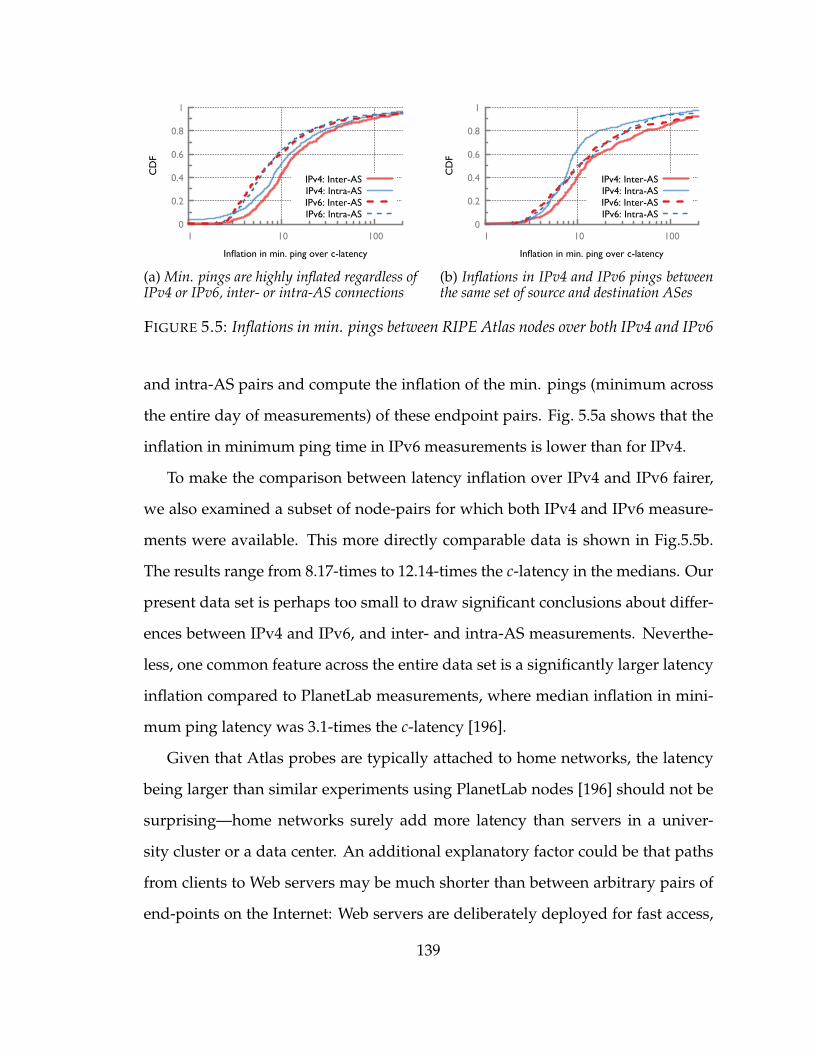
(a) Min. pings are highly inflated regardless ofIPv4 or IPv6, inter- or intra-AS connections

��

��

��

��

��

��

��

��

��

��

(b) Inflations in IPv4 and IPv6 pings betweenthe same set of source and destination ASes

FIGURE 5.5: Inflations in min. pings between RIPE Atlas nodes over both IPv4 and IPv6

and intra-AS pairs and compute the inflation of the min. pings (minimum across

the entire day of measurements) of these endpoint pairs. Fig. 5.5a shows that the

inflation in minimum ping time in IPv6 measurements is lower than for IPv4.

To make the comparison between latency inflation over IPv4 and IPv6 fairer,

we also examined a subset of node-pairs for which both IPv4 and IPv6 measure-

ments were available. This more directly comparable data is shown in Fig.5.5b.

The results range from 8.17-times to 12.14-times the c-latency in the medians. Our

present data set is perhaps too small to draw significant conclusions about differ-

ences between IPv4 and IPv6, and inter- and intra-AS measurements. Neverthe-

less, one common feature across the entire data set is a significantly larger latency

inflation compared to PlanetLab measurements, where median inflation in mini-

mum ping latency was 3.1-times the c-latency [196].

Given that Atlas probes are typically attached to home networks, the latency

being larger than similar experiments using PlanetLab nodes [196] should not be

surprising—home networks surely add more latency than servers in a univer-

sity cluster or a data center. An additional explanatory factor could be that paths

from clients to Web servers may be much shorter than between arbitrary pairs of

end-points on the Internet: Web servers are deliberately deployed for fast access,

139

��

��

��

��

��

��

FIGURE 5.6: Inflation in minimum pings between RIPE Atlas nodes as a function ofc-latency

and the Internet’s semi-hierarchical nature can make paths between arbitrary end-

points long. If this is the case, we should expect node-pairs at larger geographic

distances to experience latency inflation similar to that in the PlanetLab data set

than node-pairs that are located nearer to each other. Fig. 5.6 adds some credence

to this explanation. Here, we look at how median inflation in minimum ping la-

tency depends on the distance between the nodes.

We observe that the latency in HTML fetches from PlanetLab nodes (Section 5.3.1)

is much higher than the latency inflation in minimum pings between RIPE Atlas

nodes. This observation is most likely because of the multiplicative effect that

RTT has on the download times of Web objects. It is also worth noting that the la-

tency in minimum pings between RIPE Atlas nodes (8.17 to 12.14) is much higher

than the end-to-end latencies between CDN servers (3.1) in our longitudinal study

of server-to-server measurements (refer Chapter 2). The measurements of end-

to-end latencies of server-to-server paths are indeed similar to measurements of

ping times between the servers; no DNS resolutions or other protocol overheads

are involved. Hence, the inflation in end-to-end latencies (refer §2.9) of server-

to-server paths (3.01 over IPv4 and 3.1 over IPv6) are, perhaps, more indicative

of infrastructural latencies; ignoring the overheads from higher layers, infrastruc-

140

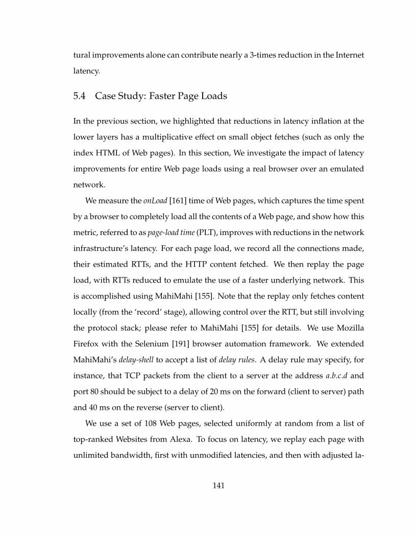
tural improvements alone can contribute nearly a 3-times reduction in the Internet

latency.

5.4 Case Study: Faster Page Loads

In the previous section, we highlighted that reductions in latency inflation at the

lower layers has a multiplicative effect on small object fetches (such as only the

index HTML of Web pages). In this section, We investigate the impact of latency

improvements for entire Web page loads using a real browser over an emulated

network.

We measure the onLoad [161] time of Web pages, which captures the time spent

by a browser to completely load all the contents of a Web page, and show how this

metric, referred to as page-load time (PLT), improves with reductions in the network

infrastructure’s latency. For each page load, we record all the connections made,

their estimated RTTs, and the HTTP content fetched. We then replay the page

load, with RTTs reduced to emulate the use of a faster underlying network. This

is accomplished using MahiMahi [155]. Note that the replay only fetches content

locally (from the ‘record’ stage), allowing control over the RTT, but still involving

the protocol stack; please refer to MahiMahi [155] for details. We use Mozilla

Firefox with the Selenium [191] browser automation framework. We extended

MahiMahi’s delay-shell to accept a list of delay rules. A delay rule may specify, for

instance, that TCP packets from the client to a server at the address a.b.c.d and

port 80 should be subject to a delay of 20 ms on the forward (client to server) path

and 40 ms on the reverse (server to client).

We use a set of 108 Web pages, selected uniformly at random from a list of

top-ranked Websites from Alexa. To focus on latency, we replay each page with

unlimited bandwidth, first with unmodified latencies, and then with adjusted la-

141

��

��

��

��

��

��

��

��

��

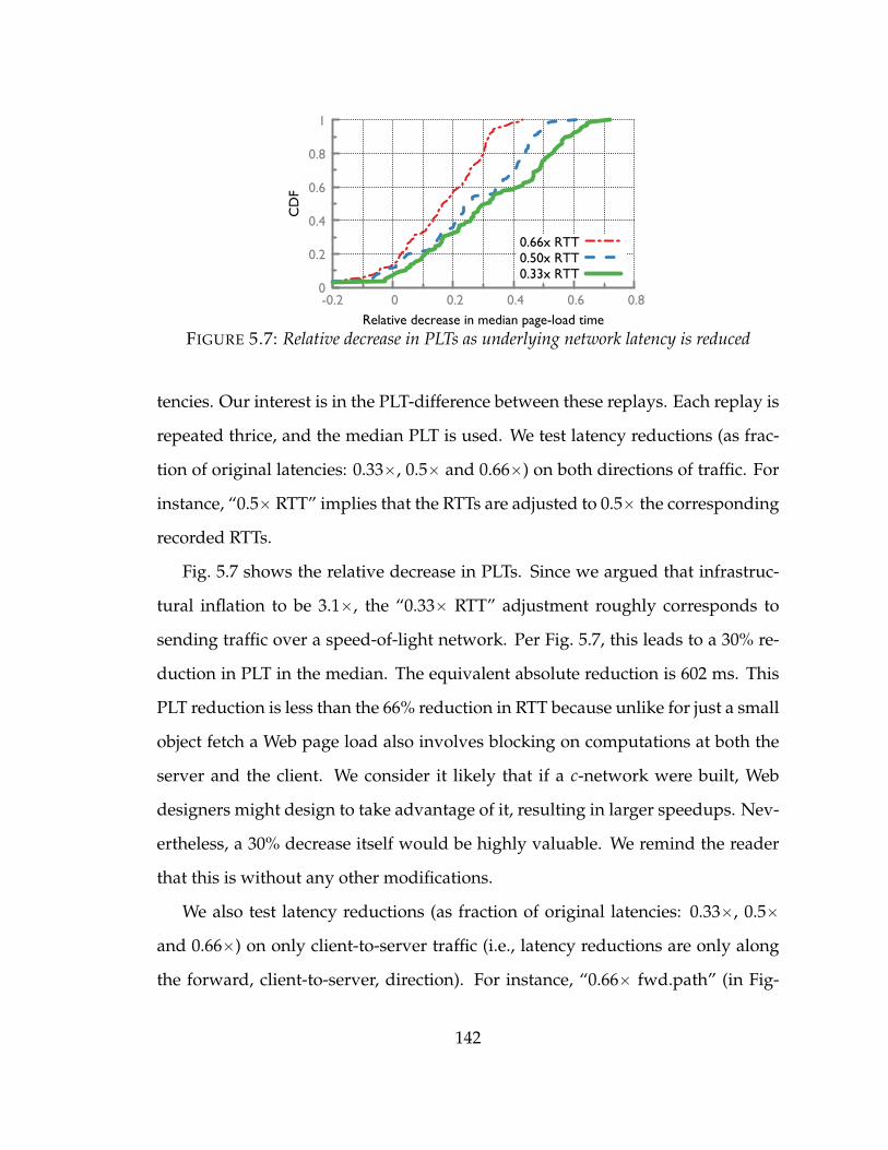
FIGURE 5.7: Relative decrease in PLTs as underlying network latency is reduced

tencies. Our interest is in the PLT-difference between these replays. Each replay is

repeated thrice, and the median PLT is used. We test latency reductions (as frac-

tion of original latencies: 0.33ˆ, 0.5ˆ and 0.66ˆ) on both directions of traffic. For

instance, “0.5ˆ RTT” implies that the RTTs are adjusted to 0.5ˆ the corresponding

recorded RTTs.

Fig. 5.7 shows the relative decrease in PLTs. Since we argued that infrastruc-

tural inflation to be 3.1ˆ, the “0.33ˆ RTT” adjustment roughly corresponds to

sending traffic over a speed-of-light network. Per Fig. 5.7, this leads to a 30% re-

duction in PLT in the median. The equivalent absolute reduction is 602 ms. This

PLT reduction is less than the 66% reduction in RTT because unlike for just a small

object fetch a Web page load also involves blocking on computations at both the

server and the client. We consider it likely that if a c-network were built, Web

designers might design to take advantage of it, resulting in larger speedups. Nev-

ertheless, a 30% decrease itself would be highly valuable. We remind the reader

that this is without any other modifications.

We also test latency reductions (as fraction of original latencies: 0.33ˆ, 0.5ˆ

and 0.66ˆ) on only client-to-server traffic (i.e., latency reductions are only along

the forward, client-to-server, direction). For instance, “0.66ˆ fwd.path” (in Fig-

142

��

��

��

��

��

��

��

��

��

FIGURE 5.8: Relative decrease in PLTs as underlying network latency is reduced onlyalong the client-to-server direction

ure 5.8) implies that only the client-to-server latencies are adjusted, and set to

0.66ˆ the recorded latency. In making these adjustments, we assume that the un-

adjusted latencies are symmetrical in each direction, i. e., 0.5ˆRTT. Per Figure 5.8,

speeding up traffic only on the forward path (“0.33ˆ fwd.path”) yields a 20% im-

provement (402 ms) in the median. This would require sending only 8.5% of the

bytes over the low-latency network in the median.

Surprisingly, Figure 5.8 and Figure 5.7 show that the CDF of ‘0.33ˆ fwd.path’

performs better compared to that of ‘0.66 ˆ RTT’; intuitively, ‘0.33x fwd.path’

should behave similar to ‘0.66ˆ RTT’. Inspecting the traffic reveals that although

the reverse path carries more traffic than the forward path, it does so in fewer

number of packets; on average, clients send more packets (but carrying less data)

to servers than that sent in the opposite direction. The 66% reduction, hence, even

if it’s only along the forward path, performs slightly better than the setup where

the RTTs are reduced by 33% in both directions.

Replaying HTTP content accurately is hard; for instance, nearly „10% of the

Web pages in our test exhibit an increase in page-load times when latencies were

decreased. Examining some of these cases reveals that even though we fetch the

same set of Web pages during the replay, the page contents show some differ-

143

ences. These differences can perhaps be attributed to non-determinism introduced

by the JavaScript components in the Web pages; for instance, advertisements on

a page may vary slightly depending on the time of day and hence, the replay

sessions might encounter requests to objects which were never observed during

the record session. These requests will fail and the failure can further introduce

non-determinism in the replays. We also should ideally model the connection de-

lays as a distribution. Regardless, our results demonstrate that latency reductions

contribute to significant improvements in page-load times and can improve the

end-user’s experience; given the non-determinism in replays, we are also, proba-

bly, under-estimating the potential benefit of network latency reduction.

5.5 Related Work

There is a large body of work on reducing Internet latency. Several efforts have fo-

cused on particular pieces; for example, [178, 224] focus on TCP handshakes; [82]

on TCP’s initial congestion window; [211] on DNS resolution; [147, 91] on routing

inflation due to BGP policy. Other work has discussed results from small scale

experiments; for example, [205] presents performance measurements for 9 pop-

ular Web sites; [106] presents DNS and TCP measurements for the most popular

100 Web sites. The WProf [212] project breaks down Web page load time for 350

Web pages into computational aspects of page rendering, as well as DNS and TCP

handshake times. Wang et al. [214] investigate latency on mobile browsers, but fo-

cus on the compute aspects rather than networking.

The 2013 Workshop on Reducing Internet Latency [11] focused on potential

mitigation techniques, with bufferbloat and active queue management being among

the centerpieces. One interesting outcome of the workshop was a qualitative chart

of latency reduction techniques, and their potential impact and feasibility (Fig. 1

144

in [114]). In a similar vein, one objective of our work is to quantify the latency

inflation and identify opportunities, e.g., infrastructural improvements, to reduce

the inflation.

There are indeed several ambitious projects related to enhancing Internet in-

frastructure, like the satellite Internet efforts of OneWeb and WorldVu [30, 98],

Google’s Loon project [10], and Facebook’s drones [129], but these are all address-

ing a different (albeit important) problem — expanding the Internet’s reach to

under-served populations. There are also efforts geared at improving bandwidth

in existing Internet markets, such as Google Fiber [6]. We hope that our work

urges greater consideration for latency in such efforts. However, so far, infras-

tructural latency has only garnered attention in niche scenarios, such as the finan-

cial markets, and isolated submarine cable projects aimed at shortening specific

routes [158, 151]. We make the case here that the role of infrastructural latency in-

flation is not well appreciated, and that it is at least as important as protocol stack

improvements for making progress on reducing latency over the Internet.

5.6 Summary

Latency is a key determinant of user experience, and it also affects the realization

and monetization of cloud services. In this chapter, we show that the latency in

Internet is far from the ideal—measurements from the edge indicate that the In-

ternet is at least 8 times slower compared to the speed of light, while in the core

latency inflation is around 3 times the c-latency. Discussions of speed in the Inter-

net often focus on bandwidth and there is hardly any mention of latency. With the

recent shift towards a cloud-computing model for deploying software, it will be

impossible to ignore the ramifications of latency inflations. The cloud amplifies

(at least) the ramifications of latency inflations: a few hundred milliseconds is all

145

that stands between the success and failure of a cloud service; users will quickly

perceive latencies as cloud services are integrated into more interactive interfaces.

We highlight that infrastructural improvements alone can offer a substantial

reduction in latencies. Singla et al. [197] propose a parallel low-latency Internet

infrastructure and urge researchers to consider “latency” as the next grand chal-

lenge in networking. In this chapter, we show how such a parallel low-latency in-

frastructure, even if it has only a limited capacity, can be immensely beneficial to

end users. Our case study of reductions in page-load times indicates that even the

availability of speed-of-light communications for only the client-to-server traffic

can yield significantly enhance user experience: based on our experiments, page-

load times decrease by over 400 ms in the median. We hope this work will encour-

age other researchers to focus more on improving Internet latency and exploiting

it to enhance the end-users’ experience.

146

6

Roadmap

You don’t understand anything until you learn it more than oneway.

— Marvin L. MinskyACM A.M. Turing Award Winner 1969

While the previous chapters discussed our current research efforts, the focus of

this chapter is to shed some light on a roadmap for future work. In the following

sections, we describe the ideas and the motivations behind them. We include

results from preliminary analysis, if required, to clearly illustrate the challenges

involved.

6.1 Dissecting End-User Experience

While researchers have been conducting client-side measurement studies to un-

derstand and estimate end-user experience [204, 202], the lack of a correlated

server-to-server study leaves many critical questions unanswered. A correlated

study entails gathering both client-side measurements and logs from the servers

involved in serving these clients with the aim of using the server-side observa-

tions to better explain the client-side measurements. For instance, the server-side

147

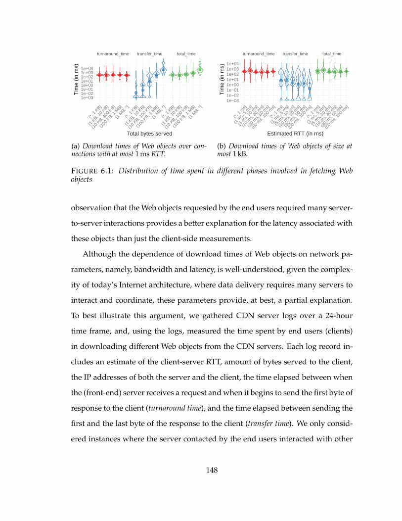
turnaround_time transfer_time total_time

1e−031e−021e−011e+001e+011e+021e+031e+04

(*, 1

KB]

(1 K

B, 10

KB]

(10

KB, 100

KB]

(100

KB, 1

MB]

(1 M

B, *]

(*, 1

KB]

(1 K

B, 10

KB]

(10

KB, 100

KB]

(100

KB, 1

MB]

(1 M

B, *]

(*, 1

KB]

(1 K

B, 10

KB]

(10

KB, 100

KB]

(100

KB, 1

MB]

(1 M

B, *]

Total bytes served

Tim

e (in

ms)

(a) Download times of Web objects over con-nections with at most 1 ms RTT.

turnaround_time transfer_time total_time

1e−031e−021e−011e+001e+011e+021e+031e+04

(*, 1

ms]

(1 m

s, 5

ms]

(5 m

s, 10

ms]

(10

ms,

30 m

s]

(30

ms,

50 m

s]

(50

ms,

100

ms]

(*, 1

ms]

(1 m

s, 5

ms]

(5 m

s, 10

ms]

(10

ms,

30 m

s]

(30

ms,

50 m

s]

(50

ms,

100

ms]

(*, 1

ms]

(1 m

s, 5

ms]

(5 m

s, 10

ms]

(10

ms,

30 m

s]

(30

ms,

50 m

s]

(50

ms,

100

ms]

Estimated RTT (in ms)

Tim

e (in

ms)

(b) Download times of Web objects of size atmost 1 kB.

FIGURE 6.1: Distribution of time spent in different phases involved in fetching Webobjects

observation that the Web objects requested by the end users required many server-

to-server interactions provides a better explanation for the latency associated with

these objects than just the client-side measurements.

Although the dependence of download times of Web objects on network pa-

rameters, namely, bandwidth and latency, is well-understood, given the complex-

ity of today’s Internet architecture, where data delivery requires many servers to

interact and coordinate, these parameters provide, at best, a partial explanation.

To best illustrate this argument, we gathered CDN server logs over a 24-hour

time frame, and, using the logs, measured the time spent by end users (clients)

in downloading different Web objects from the CDN servers. Each log record in-

cludes an estimate of the client-server RTT, amount of bytes served to the client,

the IP addresses of both the server and the client, the time elapsed between when

the (front-end) server receives a request and when it begins to send the first byte of

response to the client (turnaround time), and the time elapsed between sending the

first and the last byte of the response to the client (transfer time). We only consid-

ered instances where the server contacted by the end users interacted with other

148

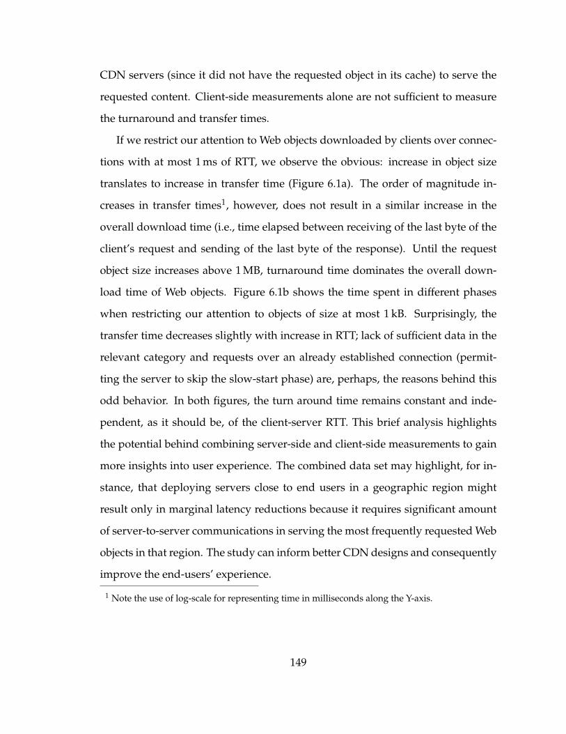
CDN servers (since it did not have the requested object in its cache) to serve the

requested content. Client-side measurements alone are not sufficient to measure

the turnaround and transfer times.

If we restrict our attention to Web objects downloaded by clients over connec-

tions with at most 1 ms of RTT, we observe the obvious: increase in object size

translates to increase in transfer time (Figure 6.1a). The order of magnitude in-

creases in transfer times1, however, does not result in a similar increase in the

overall download time (i.e., time elapsed between receiving of the last byte of the

client’s request and sending of the last byte of the response). Until the request

object size increases above 1 MB, turnaround time dominates the overall down-

load time of Web objects. Figure 6.1b shows the time spent in different phases

when restricting our attention to objects of size at most 1 kB. Surprisingly, the

transfer time decreases slightly with increase in RTT; lack of sufficient data in the

relevant category and requests over an already established connection (permit-

ting the server to skip the slow-start phase) are, perhaps, the reasons behind this

odd behavior. In both figures, the turn around time remains constant and inde-

pendent, as it should be, of the client-server RTT. This brief analysis highlights

the potential behind combining server-side and client-side measurements to gain

more insights into user experience. The combined data set may highlight, for in-

stance, that deploying servers close to end users in a geographic region might

result only in marginal latency reductions because it requires significant amount

of server-to-server communications in serving the most frequently requested Web

objects in that region. The study can inform better CDN designs and consequently

improve the end-users’ experience.

1 Note the use of log-scale for representing time in milliseconds along the Y-axis.

149

6.2 On IPv4-IPv6 Infrastructure Sharing

IP alias resolution is defined as the problem of identifying if two IP addresses be-

long to the same router and is crucial to mapping the Internet topology. While per-

forming alias resolution of two IPv4 or IPv6 addresses (i.e., determining whether

a pair of IPv4 (or IPv6) addresses are aliases of the same device or interface) is a

well-explored topic [38, 194, 122, 208, 166, 136], the question of whether an IPv4-

IPv6 IP address pair belongs to the same router or not, remains still unsolved. The

few studies that have explored IPv6-IPv6 relationships have been in the context

of nameservers [40] and Web servers [41].

While investigating the end-to-end latencies of server-to-server paths, we ob-

served (in Chapter 2) that the performance characteristics are similar over both

IPv4 and IPv6: latency inflations over IPv4 and IPv6, for instance, are very close

in value (3.01 for IPv4 and 3.1 for IPv6, in the median). Our longitudinal study

also highlight that, in a majority of instances, the end-to-end server-to-server path

latencies had no significant difference—difference in IPv4 and IPv6 latencies were

within 10 ms. These performance similarities, naturally, stress the need to under-

stand to what extent the infrastructure is shared between IPv4 and IPv6.

A careful analysis of paths where infrastructure is shared between IPv4 and

IPv6 can reveal where one protocol lags behind the other in performance and

why. In particular, the study can also identify where IPv6 performance might be

better than IPv4 and provide incentives to accelerate the adoption of IPv6. Un-

derstanding infrastructure sharing between IPv4 and IPv6 is also key towards

implementing a better IPv6 geolocation system.

150

6.3 Towards a Speedier Internet

Today, the Internet’s speed is shockingly far from the speed of light. Efforts to

design and develop a low-latency network infrastructure, a “Speed-of-Light In-

ternet”, is already underway [197]. But this speedier infrastructure, as envisioned

today, is limited in bandwidth because of technological limitations. Perhaps, we

may selectively use such a parallel infrastructure for latency-sensitive traffic. But

identifying latency-sensitive traffic, in an application-transparent manner, is hard,

if not impossible. Or perhaps, we can involve support of applications to identify

latency-sensitive traffic; this will entail developing the necessary interfaces for ap-

plications to indicate whether the traffic is latency-sensitive. These design choices

may also have implications for network neutrality.

Web pages have become increasingly complex and a typical page, today, in-

cludes more than 100 objects fetched from many different servers [7]. Even with

faster Internet infrastructure, making the Web page interactions faster may require

client-side support. Web browsers may need to be improved to prioritize objects

in a Web page to minimize the page-load times. Alternatively, Web developers

may be able to provide hints, e.g., the latency penalties incurred by different ob-

jects, or, more importantly, a rank order of objects in terms of their value to end

users, to browsers and servers to minimize page-load times. While discussions

on mechanisms for ensuring reliable Web page performance [4] are orthogonal

to the aforementioned efforts, they present an invaluable case study, highlighting

the efforts and coordination required among different platforms for implementing

portable client-side tools. With researchers now having started the initiative to-

wards lowering the Internet latency, development of client-side tools can be valu-

able in the timely realization of a low-latency Internet infrastructure.

151

7

Conclusion

What’s in your hands I think and hope is intelligence: the abilityto see the machine as more than when you were first led up to it,

that you can make it more.

— Alan J. PerlisACM A.M. Turing Award Winner 1966

During the last five years the cloud-computing model has gained tremendous

traction: Gartner, for instance, estimates the cloud services market to reach over

200 billion dollars in 2016 [95]; just five years ago, the market was estimated to be

worth „60 billion dollars [92]. Internet giants, e.g., Amazon, Microsoft, Google,

have all endorsed, at one point or another, that the cloud-computing model, in-

deed, represents the future of computing [120, 43, 29, 109]. It is this promising

approach of cloud computing that we studied in this thesis. In particular, we ana-

lyzed its ramifications on the Internet, explored fault-tolerant system designs for

better managing the cloud infrastructure, identified how a low-latency Internet

can enhance the cloud computing paradigm.

The Internet is constantly evolving and, naturally, the research presented in

this thesis may indeed diminish in “value” with the passage of time. But our ap-

proach to follow a data-driven design, insistence to rigorously vet network mea-

152

surement data sets, and interest in designing systems that fully embrace failures

should stand the test of time, and influence research methodologies in related do-

mains. We consider it an immense success if this thesis inspires further research

in this domain or others, and sincerely hope that it does.

153

Bibliography

[1] About – Google Chromebooks. https://www.google.com/chromebook/about/.

[2] Amazon Dash. https://fresh.amazon.com/dash/.

[3] Big Tap Monitoring Fabric. http://goo.gl/UHDqjT.

[4] Control Groups (cgroups for the web? https://www.igvita.com/2016/03/01/control-groups-cgroups-for-the-web/.

[5] FlowScale. http://goo.gl/WewH1U.

[6] Google Fiber. https://fiber.google.com/about/.

[7] HTTP Archive - Interesting Stats. http://httparchive.org/interesting.php.

[8] Measurement Lab (M-Lab). http://www.measurementlab.net.

[9] NEC Corporation of America. http://www.necam.com/.

[10] Project Loon. https://www.solveforx.com/loon/.

[11] Workshop on Reducing Internet Latency, 2013. http://goo.gl/kQpBCt.

[12] curl: command-line tool and library. https://curl.haxx.se, Septem-ber 1999.

[13] Big Switch Networks, Inc. http://www.bigswitch.com, 2010.

[14] PLUMgrid, Inc. http://www.plumgrid.com, 2011.

154

https://www.google.com/chromebook/about/

https://www.google.com/chromebook/about/

https://fresh.amazon.com/dash/

http://goo.gl/UHDqjT

https://www.igvita.com/2016/03/01/control-groups-cgroups-for-the-web/

https://www.igvita.com/2016/03/01/control-groups-cgroups-for-the-web/

http://goo.gl/WewH1U

https://fiber.google.com/about/

http://httparchive.org/interesting.php

http://httparchive.org/interesting.php

http://www.measurementlab.net

http://www.necam.com/

https://www.solveforx.com/loon/

http://goo.gl/kQpBCt

https://curl.haxx.se

http://www.bigswitch.com

http://www.plumgrid.com

[15] Google Compute Engine is now open to all. https://cloudplatform.googleblog.com/2013/05/google-compute-engine-is-now-open-to-all.html, May 2013.

[16] OpenDaylight: Open Source SDN Platform. https://www.opendaylight.org, 2013.

[17] Enter the Andromeda zone - Google Cloud Platform’s latest network-ing stack. https://cloudplatform.googleblog.com/2014/04/enter-andromeda-zone-google-cloud-platforms-latest-networking-stack.html, April 2014.

[18] HPE Marketplace: SDN App Store. https://saas.hpe.com/marketplace/sdn, 2014.

[19] Veriflow Systems. http://www.veriflow.net, 2016.

[20] V. K. Adhikari, Y. Guo, F. Hao, M. Varvello, V. Hilt, M. Steiner, and Z. L.Zhang. Unreeling netflix: Understanding and improving multi-CDN moviedelivery. In INFOCOM, 2012 Proceedings IEEE, pages 1620–1628, March2012.

[21] V. K. Adhikari, S. Jain, and Z.-L. Zhang. YouTube Traffic Dynamics and ItsInterplay with a Tier-1 ISP: An ISP Perspective. In Proceedings of the 10thACM SIGCOMM Conference on Internet Measurement, IMC ’10, pages 431–443, New York, NY, USA, November 2010. ACM.

[22] B. Ager, N. Chatzis, A. Feldmann, N. Sarrar, S. Uhlig, and W. Willinger.Anatomy of a Large European IXP. In Proceedings of the ACM SIGCOMM2012 Conference on Applications, Technologies, Architectures, and Protocols forComputer Communication, SIGCOMM ’12, pages 163–174, New York, NY,USA, 2012. ACM.

[23] B. Ager, W. Mühlbauer, G. Smaragdakis, and S. Uhlig. Web Content Car-tography. In Proceedings of the 2011 ACM SIGCOMM Conference on InternetMeasurement Conference, IMC ’11, pages 585–600, New York, NY, USA, 2011.ACM.

[24] B. Ager, F. Schneider, J. Kim, and A. Feldmann. Revisiting Cacheability inTimes of User Generated Content. In INFOCOM IEEE Conference on Com-puter Communications Workshops , 2010, pages 1–6, March 2010.

155

https://cloudplatform.googleblog.com/2013/05/google-compute-engine-is-now-open-to-all.html



https://www.opendaylight.org

https://www.opendaylight.org

https://cloudplatform.googleblog.com/2014/04/enter-andromeda-zone-google-cloud-platforms-latest-networking-stack.html



https://saas.hpe.com/marketplace/sdn

https://saas.hpe.com/marketplace/sdn

http://www.veriflow.net

[25] Akamai. State of the internet, q1 2016: Americas highlights. https://www.akamai.com/us/en/multimedia/documents/state-of-the-internet/akamai-q1-2016-state-of-the-internet-infographic-americas.pdf, April 2016.

[26] Akamai Technologies, Inc. EdgePlatform. http://www4.akamai.com/html/technology/products/edgescape.html, 2013.

[27] A. Akella, S. Seshan, and A. Shaikh. An Empirical Evaluation of Wide-areaInternet Bottlenecks. In Proceedings of the 3rd ACM SIGCOMM Conference onInternet Measurement, IMC ’03, pages 101–114, New York, NY, USA, 2003.ACM.

[28] Alexa. The top 500 sites on the Web (By Country). http://www.alexa.com/topsites/countries.

[29] K. Allen. 5 bold cloud predictions from IBM Distinguished En-gineers. http://www.thoughtsoncloud.com/2015/10/5-bold-cloud-predictions-from-ibm-distinguished-engineers/, Oc-tober 2013.

[30] N. Allen. Elon Musk announces ’space Internet’ plan. http://www.telegraph.co.uk/news/worldnews/northamerica/usa/11353782/Elon-Musk-announces-space-Internet-plan.html,January 2015.

[31] M. Allman. On Changing the Culture of Empirical Internet Assessment.SIGCOMM Comput. Commun. Rev., 43(3):78–83, Jul 2013.

[32] Alphabet. Google Inc. Announces Second Quarter 2015 Results.https://abc.xyz/investor/news/earnings/2015/Q2_google_earnings/, July 2015.

[33] Alphabet. Alphabet Announces First Quarter 2016 Results. https://abc.xyz/investor/news/earnings/2016/Q1_alphabet_earnings/,April 2016.

[34] Alphabet. Alphabet Announces Second Quarter 2016 Results. https://abc.xyz/investor/news/earnings/2016/Q2_alphabet_earnings/, July 2016.

[35] AMS-IX. Ams-ix standard service level agreement. https://ams-ix.net/services-pricing/service-level-agreement, 2015.

156

https://www.akamai.com/us/en/multimedia/documents/state-of-the-internet/akamai-q1-2016-state-of-the-internet-infographic-americas.pdf




http://www4.akamai.com/html/technology/products/edgescape.html

http://www4.akamai.com/html/technology/products/edgescape.html

http://www.alexa.com/topsites/countries

http://www.alexa.com/topsites/countries

http://www.thoughtsoncloud.com/2015/10/5-bold-cloud-predictions-from-ibm-distinguished-engineers/

http://www.thoughtsoncloud.com/2015/10/5-bold-cloud-predictions-from-ibm-distinguished-engineers/

http://www.telegraph.co.uk/news/worldnews/northamerica/usa/11353782/Elon-Musk-announces-space-Internet-plan.html



https://abc.xyz/investor/news/earnings/2015/Q2_google_earnings/

https://abc.xyz/investor/news/earnings/2015/Q2_google_earnings/

https://abc.xyz/investor/news/earnings/2016/Q1_alphabet_earnings/





https://ams-ix.net/services-pricing/service-level-agreement

https://ams-ix.net/services-pricing/service-level-agreement

[36] M. J. Arif, S. Karunasekera, and S. Kulkarni. GeoWeight: Internet Host Ge-olocation Based on a Probability Model for Latency Measurements. In Pro-ceedings of the Thirty-Third Australasian Conferenc on Computer Science - Vol-ume 102, ACSC ’10, pages 89–98, Darlinghurst, Australia, Australia, January2010. Australian Computer Society, Inc.

[37] B. Augustin, X. Cuvellier, B. Orgogozo, F. Viger, T. Friedman, M. Latapy,C. Magnien, and R. Teixeira. Avoiding Traceroute Anomalies with ParisTraceroute. In Proceedings of the 6th ACM SIGCOMM Conference on InternetMeasurement, IMC ’06, pages 153–158, New York, NY, USA, October 2006.ACM.

[38] A. Bender, R. Sherwood, and N. Spring. Fixing Ally’s Growing Pains withVelocity Modeling. In IMC ’08: Proceedings of the 8th ACM SIGCOMM con-ference on Internet measurement, pages 337–342, New York, NY, USA, 2008.ACM.

[39] P. Berde, M. Gerola, J. Hart, Y. Higuchi, M. Kobayashi, T. Koide, B. Lantz,B. O’Connor, P. Radoslavov, W. Snow, and G. Parulkar. ONOS: Towards anOpen, Distributed SDN OS. HotSDN, 2014.

[40] A. Berger, N. Weaver, R. Beverly, and L. Campbell. Internet NameserverIPv4 and IPv6 Address Relationships. In Proceedings of the 2013 Conferenceon Internet Measurement Conference, IMC ’13, pages 91–104, New York, NY,USA, 2013. ACM.

[41] R. Beverly and A. Berger. Server Siblings: Identifying Shared IPv4/IPv6 In-frastructure Via Active Fingerprinting, pages 149–161. Springer InternationalPublishing, Cham, 2015.

[42] Big Switch Networks, Inc. Project Floodlight: Open Source Soft-ware for Building Software-Defined Networks. http://www.projectfloodlight.org, 2012.

[43] M. Brown. Microsoft: ’The Future is Now’ for Cloud Computing.http://mspmentor.net/infocenter-cloud-based-file-sharing/051614/microsoft-future-now-cloud-computing,May 2014.

[44] J. Brutlag. Speed Matters for Google Web Search. http://services.google.com/fh/files/blogs/google_delayexp.pdf, June 2009.

[45] S. M. Burke and T. Solc. Unidecode, 2013.

157

http://www.projectfloodlight.org

http://www.projectfloodlight.org

http://mspmentor.net/infocenter-cloud-based-file-sharing/051614/microsoft-future-now-cloud-computing

http://mspmentor.net/infocenter-cloud-based-file-sharing/051614/microsoft-future-now-cloud-computing

http://services.google.com/fh/files/blogs/google_delayexp.pdf

http://services.google.com/fh/files/blogs/google_delayexp.pdf

[46] R. Bush, O. Maennel, M. Roughan, and S. Uhlig. Internet Optometry: As-sessing the Broken Glasses in Internet Reachability. In Proceedings of the9th ACM SIGCOMM Conference on Internet Measurement Conference, IMC ’09,pages 242–253, New York, NY, USA, 2009. ACM.

[47] CAIDA. Archipelago measurement infrastructure. http://www.caida.org/projects/ark/, 2013.

[48] CAIDA. AS Rank: AS Ranking. http://as-rank.caida.org/,02/19/2013 2013.

[49] M. Calder, X. Fan, Z. Hu, E. Katz-Bassett, J. Heidemann, and R. Govindan.Mapping the Expansion of Google’s Serving Infrastructure. In Proceedings ofthe 2013 Conference on Internet Measurement Conference, IMC ’13, pages 313–326, New York, NY, USA, 2013. ACM.

[50] G. Candea, S. Kawamoto, Y. Fujiki, G. Friedman, and A. Fox. Microreboot— A Technique for Cheap Recovery. OSDI, 2004.

[51] M. Canini, P. Kuznetsov, D. Levin, and S. Schmid. Software TransactionalNetworking: Concurrent and Consistent Policy Composition. HotSDN,2013.

[52] M. Canini, D. Venzano, P. Perešíni, D. Kostic, and J. Rexford. A NICE Wayto Test Openflow Applications. NSDI, 2012.

[53] N. Caruso. A Distributed System For Large-Scale Geolocalization Of Inter-net Hosts. diploma thesis, Cornell University, Ithaca, NY, 2011.

[54] CENGN. CENGN Blog: SDN Hackathon. http://www.cengn.ca/sdn-hackathon/, September 2015.

[55] U. S. o. A. Census Bureau. TIGER/Line Shapefiles. http://www.census.gov/geo/www/tiger/shp.html, 2012.

[56] B. Chandrasekaran, M. Bai, M. Schoenfield, A. Berger, N. Caruso,G. Economou, S. Gilliss, B. Maggs, K. Moses, D. Duff, K.-C. Ng, E. G. Sirer,R. Weber, and B. Wong. Alidade: IP Geolocation without Active Probing.Technical Report CS-TR-2015-001, Duke University, January 2015.

[57] B. Chandrasekaran and T. Benson. Tolerating SDN Application Failureswith LegoSDN. In Proceedings of the 13th ACM Workshop on Hot Topics inNetworks, HotNets-XIII, pages 22:1–22:7, New York, NY, USA, 2014. ACM.

158

http://www.caida.org/projects/ark/

http://www.caida.org/projects/ark/

http://as-rank.caida.org/

http://www.cengn.ca/sdn-hackathon/

http://www.cengn.ca/sdn-hackathon/

http://www.census.gov/geo/www/tiger/shp.html

http://www.census.gov/geo/www/tiger/shp.html

[58] B. Chandrasekaran and T. Benson. Tolerating SDN Application Failureswith LegoSDN. HotNets, 2014.

[59] B. Chandrasekaran, G. Smaragdakis, A. Berger, M. Luckie, and K.-C. Ng. AServer-to-Server View of the Internet. In Proceedings of ACM CoNEXT 2015,Heidelberg, Germany, December 2015.

[60] B. Chandrasekaran, B. Tschaen, and T. Benson. Isolating and ToleratingSDN Application Failures with LegoSDN. In Proceedings of the 2nd ACMSIGCOMM Symposium on Software Defined Networking Research, SOSR ’16.ACM, March 2016.

[61] H. Chang, S. Jamin, and W. Willinger. Inferring AS-level Internet topologyfrom router-level path traces. volume 4526, pages 196–207, 2001.

[62] J. Chao. Brocade Embraces OpenFlow 1.3. http://www.enterprisenetworkingplanet.com/nethub/brocade-embraces-openflow-1.3.html, March 2014.

[63] N. Chatzis, G. Smaragdakis, A. Feldmann, and W. Willinger. There is Moreto IXPs Than Meets the Eye. SIGCOMM Comput. Commun. Rev., 43(5):19–28,Nov 2013.

[64] N. Chatzis, G. Smaragdakis, A. Feldmann, and W. Willinger. Quo VadisOpen-IX? SIGCOMM Comput. Commun. Rev., 45(1):12–18, Jan 2015.

[65] F. Chen, R. K. Sitaraman, and M. Torres. End-User Mapping: Next Genera-tion Request Routing for Content Delivery. In Proceedings of the 2015 ACMConference on Special Interest Group on Data Communication, SIGCOMM ’15,pages 167–181, New York, NY, USA, 2015. ACM.

[66] K. Chen, D. R. Choffnes, R. Potharaju, Y. Chen, F. E. Bustamante, D. Pei, andY. Zhao. Where the Sidewalk Ends: Extending the Internet As Graph Us-ing Traceroutes from P2P Users. In Proceedings of the 5th International Con-ference on Emerging Networking Experiments and Technologies, CoNEXT ’09,pages 217–228, New York, NY, USA, December 2009. ACM.

[67] E. Chew, R. Zimmermann, A. Sawchuk, C. Papadopoulos, C. Kyriakakis,C. Tanoue, D. Desai, M. Pawar, R. Sinha, and W. Meyer. A Second Reporton the User Experiments in the Distributed Immersive Performance Project.In Proceedings of the 5th Open Workshop of MUSICNETWORK: Integration ofMusic in Multimedia Applications, July 2005.

159

http://www.enterprisenetworkingplanet.com/nethub/brocade-embraces-openflow-1.3.html



[68] B. Chun, D. Culler, T. Roscoe, A. Bavier, L. Peterson, M. Wawrzoniak, andM. Bowman. PlanetLab: An Overlay Testbed for Broad-coverage Services.SIGCOMM Comput. Commun. Rev., 33(3):3–12, Jul 2003.

[69] Cisco. OpenDaylight BGP and PCEP (Pathman) Apps. https://github.com/CiscoDevNet/Opendaylight-BGP-Pathman-apps,September 2015.

[70] R. S. F. Community. Ryu: Component-based Software-defined NetworkingFramework. , 2012.

[71] Checkpoint/Restore In Userspace (CRIU). http://goo.gl/OMb5K.

[72] E. Cuervo. Enhancing Mobile Devices through Code Offload. PhD thesis, DukeUniversity, 2012.

[73] J. Czyz, M. Allman, J. Zhang, S. Iekel-Johnson, E. Osterweil, and M. Bailey.Measuring IPv6 Adoption. In Proceedings of the 2014 ACM Conference onSIGCOMM, SIGCOMM ’14, pages 87–98, New York, NY, USA, 2014. ACM.

[74] F. Dabek, R. Cox, F. Kaashoek, and R. Morris. Vivaldi: A Decentralized Net-work Coordinate System. In ACM SIGCOMM, pages 15–26, August 2004.

[75] H. T. Dang, D. Sciascia, M. Canini, F. Pedone, and R. Soulé. NetPaxos: Con-sensus at Network Speed. SOSR, 2015.

[76] L. Deng and A. Kuzmanovic. Monitoring persistently congested Internetlinks. In Network Protocols, 2008. ICNP 2008. IEEE International Conference on,pages 167–176, Oct 2008.

[77] A. Dhamdhere and C. Dovrolis. Twelve Years in the Evolution of the Inter-net Ecosystem. IEEE/ACM Transactions on Networking, 19(5):1420–1433, Oct2011.

[78] L. Dignan. Google presses algorithm, cloud advantage vs. Ap-ple, rivals. http://www.zdnet.com/article/google-presses-algorithm-cloud-advantage-vs-apple-rivals/, May 2013.

[79] M. Dischinger, M. Marcon, S. Guha, K. P. Gummadi, R. Mahajan, andS. Saroiu. Glasnost: Enabling End Users to Detect Traffic Differentiation.In Proceedings of the 7th USENIX Conference on Networked Systems Design andImplementation, NSDI’10, pages 27–27, Berkeley, CA, USA, 2010. USENIXAssociation.

160

https://github.com/CiscoDevNet/Opendaylight-BGP-Pathman-apps

https://github.com/CiscoDevNet/Opendaylight-BGP-Pathman-apps

http://goo.gl/OMb5K

http://www.zdnet.com/article/google-presses-algorithm-cloud-advantage-vs-apple-rivals/

http://www.zdnet.com/article/google-presses-algorithm-cloud-advantage-vs-apple-rivals/

[80] F. Dobrian, V. Sekar, A. Awan, I. Stoica, D. Joseph, A. Ganjam, J. Zhan, andH. Zhang. Understanding the Impact of Video Quality on User Engage-ment. In Proceedings of the ACM SIGCOMM 2011 Conference, SIGCOMM ’11,pages 362–373, New York, NY, USA, 2011. ACM.

[81] I. Drago, M. Mellia, M. M. Munafo, A. Sperotto, R. Sadre, and A. Pras. InsideDropbox: Understanding Personal Cloud Storage Services. In Proceedings ofthe 2012 ACM Conference on Internet Measurement Conference, IMC ’12, pages481–494, New York, NY, USA, 2012. ACM.

[82] N. Dukkipati, T. Refice, Y. Cheng, J. Chu, T. Herbert, A. Agarwal, A. Jain,and N. Sutin. An Argument for Increasing TCP’s Initial Congestion Win-dow. SIGCOMM Comput. Commun. Rev., 40(3):26–33, Jun 2010.

[83] A. Dwaraki, S. Seetharaman, S. Natarajan, and T. Wolf. GitFlow: Flow Re-vision Management for Software-defined Networks. SOSR, 2015.

[84] H. Edelsbrunner, D. Kirkpatrick, and R. Seidel. On the Shape of a Set ofPoints in the Plane. IEEE Trans. Inf. Theor., 29(4):551–559, Sep 2006.

[85] B. Eriksson, P. Barford, B. Maggs, and R. Nowak. Posit: a lightweight ap-proach for IP geolocation. SIGMETRICS Perform. Eval. Rev., 40(2):2–11, Oct2012.

[86] B. Eriksson, P. Barford, J. Sommers, and R. Nowak. A Learning-Based Ap-proach for IP Geolocation. In Proc. of the 11th International Conf. on Passiveand Active Measurement, PAM’10, pages 171–180, Berlin, Heidelberg, April2010. Springer-Verlag.

[87] T. Flach, N. Dukkipati, A. Terzis, B. Raghavan, N. Cardwell, Y. Cheng,A. Jain, S. Hao, E. Katz-Bassett, and R. Govindan. Reducing Web Latency:The Virtue of Gentle Aggression. In Proceedings of the ACM SIGCOMM 2013Conference on SIGCOMM, SIGCOMM ’13, pages 159–170, New York, NY,USA, 2013. ACM.

[88] N. Foster, M. J. Freedman, R. Harrison, J. Rexford, M. L. Meola, andD. Walker. Frenetic: A High-level Language for OpenFlow Networks.PRESTO, 2010.

[89] M. J. Freedman, M. Vutukuru, N. Feamster, and H. Balakrishnan. Geo-graphic Locality of IP Prefixes. In Proceedings of the 5th ACM SIGCOMMconference on Internet Measurement, IMC ’05, pages 13–13, Berkeley, CA, USA,2005. USENIX Association.

161

[90] E. Frieberg. Google and VMware Double Down on Desktop as a Serviceas Windows XP Support Ends. http://blogs.vmware.com/euc/2014/04/google-vmware-double-desktop-service-windows-xp-support-ends.html, April 2014.

[91] L. Gao and F. Wang. The extent of AS path inflation by routing policies. InGlobal Telecommunications Conference, 2002. GLOBECOM ’02. IEEE, volume 3,pages 2180–2184 vol.3, Nov 2002.

[92] Gartner. Gartner Says Worldwide Cloud Services Market to Surpass $68 Bil-lion in 2010. http://www.gartner.com/newsroom/id/1389313, June2010.

[93] Gartner. Gartner Says the Internet of Things Installed Base Will Grow to26 Billion Units By 2020. http://www.gartner.com/newsroom/id/2636073, December 2013.

[94] Gartner. Gartner Identifies the Top 10 Strategic Technology Trends for 2015.http://www.gartner.com/newsroom/id/2867917, October 2014.

[95] Gartner. Gartner Says Worldwide Public Cloud Services Market Is Forecastto Reach $204 Billion in 2016. http://www.gartner.com/newsroom/id/3188817, January 2016.

[96] A. Gember, R. Grandl, A. Anand, T. Benson, and A. Akella. Stratos: VirtualMiddleboxes as First-Class Entities. Technical Report TR1771, University ofWisconsin-Madison, June 2012.

[97] A. Gember-Jacobson, R. Viswanathan, C. Prakash, R. Grandl, J. Khalid,S. Das, and A. Akella. OpenNF: Enabling Innovation in Network FunctionControl. SIGCOMM, 2014.

[98] M. Geuss. Satellite Internet: meet the hip new investment for RichardBranson, Elon Musk. http://arstechnica.com/business/2015/01/satellite-internet-meet-the-hip-new-investment-for-richard-branson-elon-musk/, January 2015.

[99] P. Gill, Y. Ganjali, B. Wong, and D. Lie. Dude, where’s that IP? Circumvent-ing measurement-based IP geolocation. In Proceedings of the 19th USENIXconference on Security, USENIX Security’10, pages 16–16, Berkeley, CA, USA,2010. USENIX Association.

162

http://blogs.vmware.com/euc/2014/04/google-vmware-double-desktop-service-windows-xp-support-ends.html



http://www.gartner.com/newsroom/id/1389313






http://arstechnica.com/business/2015/01/satellite-internet-meet-the-hip-new-investment-for-richard-branson-elon-musk/



[100] A. Greenberg. Microsoft Showcases Software Defined Networking In-novation at SIGCOMM. https://azure.microsoft.com/en-us/blog/microsoft-showcases-software-defined-networking-innovation-at-sigcomm-v2/, August 2015.

[101] I. Grigorik. Latency: The New Web Performance Bottleneck.https://www.igvita.com/2012/07/19/latency-the-new-web-performance-bottleneck/, July 2012.

[102] I. Grigorik. High Performance Browser Networking. O’Reilly Media, 1 edition,September 2013.

[103] B. Gueye, A. Ziviani, M. Crovella, and S. Fdida. Constraint-Based Geoloca-tion of Internet Hosts. In ACM Internet Measurement Conference, Taormina,Sicily, Italy, October 2004.

[104] C. Guo, Y. Liu, W. Shen, H. Wang, Q. Yu, and Y. Zhang. Mining the Weband the Internet for Accurate IP Address Geolocations. In INFOCOM 2009,IEEE, pages 2841–2845, 2009.

[105] K. Ha, P. Pillai, G. Lewis, S. Simanta, S. Clinch, N. Davies, and M. Satya-narayanan. The Impact of Mobile Multimedia Applications on Data CenterConsolidation. In Cloud Engineering (IC2E), 2013 IEEE International Confer-ence on, pages 166–176, March 2013.

[106] M. A. Habib and M. Abrams. Analysis of Sources of Latency in Down-loading Web Pages. In Proceedings of WebNet 2000 - World Conference on theWWW and Internet, San Antonio, Texas, USA, October 30 - November 4, 2000,pages 227–232, 2000.

[107] N. Handigol, B. Heller, V. Jeyakumar, D. Mazières, and N. McKeown. IKnow What Your Packet Did Last Hop: Using Packet Histories to Trou-bleshoot Networks. NSDI, 2014.

[108] B. Heller, C. Scott, N. McKeown, S. Shenker, A. Wundsam, H. Zeng,S. Whitlock, V. Jeyakumar, N. Handigol, J. McCauley, K. Zarifis, andP. Kazemian. Leveraging SDN Layering to Systematically Troubleshoot Net-works. HotSDN, 2013.

[109] T. Herbert. Vint Cerf Envisions Interoperable Clouds Driving CollaborativeComputing, Analytics. http://data-informed.com/vint-cerf-envisions-interoperable-clouds-driving-collaborative-computing-analytics/, January 2013.

163

https://azure.microsoft.com/en-us/blog/microsoft-showcases-software-defined-networking-innovation-at-sigcomm-v2/



https://www.igvita.com/2012/07/19/latency-the-new-web-performance-bottleneck/

https://www.igvita.com/2012/07/19/latency-the-new-web-performance-bottleneck/

http://data-informed.com/vint-cerf-envisions-interoperable-clouds-driving-collaborative-computing-analytics/



[110] R. Hijmans. Global Administrative Areas. http://www.gadm.org/, 2012.

[111] T. Holterbach, C. Pelsser, R. Bush, and L. Vanbever. Quantifying Interfer-ence Between Measurements on the RIPE Atlas Platform. In Proceedings ofthe 2015 ACM Conference on Internet Measurement Conference, IMC ’15, pages437–443, New York, NY, USA, 2015. ACM.

[112] Y. Hyun, A. Broido, and k. claffy. Traceroute and BGP AS Path Incon-gruities. Technical report, Cooperative Association for Internet Data Analy-sis (CAIDA), Mar 2003.

[113] Intel. Chip Shot: Intel Embraces SDN at IDF. https://newsroom.intel.com/chip-shots/chip-shot-intel-embraces-sdn-at-idf/, September 2012.

[114] Internet Society. Workshop on Reducing Internet Latency, 2013 — Report.https://www.internetsociety.org/sites/default/files/Workshop%20on%20Reducing%20Internet%20Latency-1.2.pdf,September 2013.

[115] IP2Location.com. IP2Location. http://www.ip2location.com/, 2013.

[116] S. Jain, A. Kumar, S. Mandal, J. Ong, L. Poutievski, A. Singh, S. Venkata,J. Wanderer, J. Zhou, M. Zhu, J. Zolla, U. Hölzle, S. Stuart, and A. Vahdat.B4: Experience with a Globally-Deployed Software Defined WAN. In Pro-ceedings of the ACM SIGCOMM 2013 Conference on SIGCOMM, SIGCOMM’13, pages 3–14, New York, NY, USA, August 2013. ACM.

[117] A. Kadav, M. J. Renzelmann, and M. M. Swift. Fine-grained fault toleranceusing device checkpoints. ASPLOS, 2013.

[118] N. Katta, H. Zhang, M. Freedman, and J. Rexford. Ravana: Controller Fault-tolerance in Software-defined Networking. In Proceedings of the 1st ACMSIGCOMM Symposium on Software Defined Networking Research, SOSR ’15,pages 4:1–4:12, New York, NY, USA, 2015. ACM.

[119] E. Katz-Bassett, J. P. John, A. Krishnamurthy, D. Wetherall, T. Anderson, andY. Chawathe. Towards IP Geolocation Using Delay and Topology Measure-ments. In Proceedings of the 6th ACM SIGCOMM conference on Internet mea-surement, IMC ’06, pages 71–84, New York, NY, USA, October 2006. ACM.

[120] M. Kavis. Google’s Glimpse Into The Future of Cloud Comput-ing. http://www.cloudtp.com/2016/03/25/google-provides-glimpse-future-cloud/, March 2016.

164

http://www.gadm.org/

https://newsroom.intel.com/chip-shots/chip-shot-intel-embraces-sdn-at-idf/



https://www.internetsociety.org/sites/default/files/Workshop%20on%20Reducing%20Internet%20Latency-1.2.pdf

https://www.internetsociety.org/sites/default/files/Workshop%20on%20Reducing%20Internet%20Latency-1.2.pdf

http://www.ip2location.com/

http://www.cloudtp.com/2016/03/25/google-provides-glimpse-future-cloud/

http://www.cloudtp.com/2016/03/25/google-provides-glimpse-future-cloud/

[121] M. Kelly. 96 percent of Google’s revenue is advertising, who buys it? http://venturebeat.com/2012/01/29/google-advertising/, January2012.

[122] K. Keys. Internet-Scale IP Alias Resolution Techniques. SIGCOMM Comput.Commun. Rev., 40(1):50–55, Jan 2010.

[123] A. Khan, T. Kwon, H.-c. Kim, and Y. Choi. AS-level Topology CollectionThrough Looking Glass Servers. In Proceedings of the 2013 Conference on In-ternet Measurement Conference, IMC ’13, pages 235–242, New York, NY, USA,2013. ACM.

[124] A. Khurshid, X. Zou, W. Zhou, M. Caesar, and P. B. Godfrey. VeriFlow:Verifying Network-wide Invariants in Real Time. NSDI, 2013.

[125] T. Koponen, M. Casado, N. Gude, J. Stribling, L. Poutievski, M. Zhu, R. Ra-manathan, Y. Iwata, H. Inoue, T. Hama, and S. Shenker. Onix: A DistributedControl Platform for Large-scale Production Networks. OSDI, 2010.

[126] M. Kuzniar, P. Peresini, M. Canini, D. Venzano, and D. Kostic. A SOFT Wayfor Openflow Switch Interoperability Testing. CoNEXT, 2012.

[127] S. Laki, P. Mátray, P. Hága, T. Sebok, I. Csabai, and G. Vattay. Spotter: AModel Based Active Geolocation Service. In IEEE INFOCOM, April 2011.

[128] B. Lantz, B. Heller, and N. McKeown. A Network in a Laptop: Rapid Proto-typing for Software-defined Networks. HotNets, 2010.

[129] I. Lapowsky. Facebook Lays Out Its Roadmap for Creating Internet-Connected Drones. http://www.wired.com/2014/09/facebook-drones-2/, September 2014.

[130] T. Leighton. Improving Performance on the Internet. Queue, 6(6):20–29, Oct2008.

[131] S. Levy. Going With the Flow: Google’s Secret Switch to the Next Wave ofNetworking. http://www.wired.com/2012/04/going-with-the-flow-google/, April 2012.

[132] A. Li, X. Yang, S. Kandula, and M. Zhang. CloudCmp: Comparing PublicCloud Providers. In Proceedings of the 10th ACM SIGCOMM Conference onInternet Measurement, IMC ’10, pages 1–14, New York, NY, USA, 2010. ACM.

165

http://venturebeat.com/2012/01/29/google-advertising/

http://venturebeat.com/2012/01/29/google-advertising/

http://www.wired.com/2014/09/facebook-drones-2/

http://www.wired.com/2014/09/facebook-drones-2/

http://www.wired.com/2012/04/going-with-the-flow-google/

http://www.wired.com/2012/04/going-with-the-flow-google/

[133] J. Liddle. Amazon found every 100ms of latency cost them 1% in sales.. http://blog.gigaspaces.com/amazon-found-every-100ms-of-latency-cost-them-1-in-sales/, August 2008.

[134] A. Lodhi, A. Dhamdhere, and C. Dovrolis. Open peering by Internet transitproviders: Peer preference or peer pressure? In IEEE INFOCOM 2014 - IEEEConference on Computer Communications, pages 2562–2570, April 2014.

[135] S. Lohr. For Impatient Web Users, an Eye Blink Is Just TooLong to Wait. http://www.nytimes.com/2012/03/01/technology/impatient-web-users-flee-slow-loading-sites.html, Febru-ary 2012.

[136] M. Luckie, R. Beverly, W. Brinkmeyer, and k. claffy. Speedtrap: Internet-scale IPv6 Alias Resolution. In Proceedings of the 2013 Conference on InternetMeasurement Conference, IMC ’13, pages 119–126, New York, NY, USA, 2013.ACM.

[137] M. Luckie, A. Dhamdhere, k. claffy, and D. Murrell. Measured Impact ofCrooked Traceroute. SIGCOMM Comput. Commun. Rev., 41(1):14–21, Jan2011.

[138] M. Luckie, A. Dhamdhere, D. Clark, B. Huffaker, and k. claffy. Challengesin Inferring Internet Interdomain Congestion. In Proceedings of the 2014 Con-ference on Internet Measurement Conference, IMC ’14, pages 15–22, New York,NY, USA, 2014. ACM.

[139] M. Luckie, B. Huffaker, A. Dhamdhere, V. Giotsas, and k. claffy. AS Relation-ships, Customer Cones, and Validation. In Proceedings of the 2013 Conferenceon Internet Measurement Conference, IMC ’13, pages 243–256, New York, NY,USA, 2013. ACM.

[140] M. Luckie, B. Huffaker, A. Dhamdhere, V. Giotsas, and k. claffy. As relation-ships, customer cones, and validation. In Proceedings of the 2013 Conferenceon Internet Measurement Conference, IMC ’13, pages 243–256, New York, NY,USA, 2013. ACM.

[141] H. V. Madhyastha, T. Isdal, M. Piatek, C. Dixon, T. Anderson, A. Krish-namurthy, and A. Venkataramani. iPlane: An Information Plane for Dis-tributed Services. In OSDI ’06: Proceedings of the 7th symposium on Oper-ating systems design and implementation, pages 367–380, Berkeley, CA, USA,November 2006. USENIX Association.

166

http://blog.gigaspaces.com/amazon-found-every-100ms-of-latency-cost-them-1-in-sales/

http://blog.gigaspaces.com/amazon-found-every-100ms-of-latency-cost-them-1-in-sales/

http://www.nytimes.com/2012/03/01/technology/impatient-web-users-flee-slow-loading-sites.html

http://www.nytimes.com/2012/03/01/technology/impatient-web-users-flee-slow-loading-sites.html

[142] Z. M. Mao, J. Rexford, J. Wang, and R. H. Katz. Towards an Accurate AS-level Traceroute Tool. In Proceedings of the 2003 Conference on Applications,Technologies, Architectures, and Protocols for Computer Communications, SIG-COMM ’03, pages 365–378, New York, NY, USA, 2003. ACM.

[143] MaxMind, Inc. GeoIP City. http://www.maxmind.com/en/geolocation_landing, 2013.

[144] J. McCarthy. Reminiscences on the History of Time Sharing.http://www-formal.stanford.edu/jmc/history/timesharing/timesharing.html, 1983.

[145] J. Miserez, P. Bielik, A. El-Hassany, L. Vanbever, and M. Vechev. SDNRacer:Detecting Concurrency Violations in Software-defined Networks. SOSR,2015.

[146] D. R. Morrison. PATRICIA: Practical Algorithm To Retrieve InformationCoded in Alphanumeric. J. ACM, 15(4):514–534, oct 1968.

[147] W. Mühlbauer, S. Uhlig, A. Feldmann, O. Maennel, B. Quoitin, and B. Fu.Impact of routing parameters on route diversity and path inflation. Com-puter Networks, 54(14):2506 – 2518, 2010.

[148] R. NCC. About RIPE Atlas. https://atlas.ripe.net/about/, Octo-ber 2011.

[149] R. NCC. RIPE Atlas FAQ: Are the locations of probes made pub-lic? https://atlas.ripe.net/about/faq/#are-the-locations-of-probes-made-public, 2015.

[150] NEC. NEC Contributes Network Virtualization to OpenDaylight’s Hy-drogen Release. http://www.nec.com/en/press/201402/global_20140204_02.html, February 2014.

[151] NEC. SEA-US: Global Consortium to Build Cable System Connecting In-donesia, the Philippines, and the United States. http://www.nec.com/en/press/201408/global_20140828_04.html, August 2014.

[152] T. Nelson, D. Yu, Y. Li, R. Fonseca, and S. Krishnamurthi. Simon: ScriptableInteractive Monitoring for SDNs. SOSR, 2015.

[153] Net Industries, LLC. HostIP.info. http://www.hostip.info, 2013.

167

http://www.maxmind.com/en/geolocation_landing

http://www.maxmind.com/en/geolocation_landing

http://www-formal.stanford.edu/jmc/history/timesharing/timesharing.html

http://www-formal.stanford.edu/jmc/history/timesharing/timesharing.html

https://atlas.ripe.net/about/

https://atlas.ripe.net/about/faq/#are-the-locations-of-probes-made-public

https://atlas.ripe.net/about/faq/#are-the-locations-of-probes-made-public

http://www.nec.com/en/press/201402/global_20140204_02.html




http://www.hostip.info

[154] Netflix. Netflix Open Connect. https://openconnect.itp.netflix.com, 2015.

[155] R. Netravali, A. Sivaraman, S. Das, A. Goyal, K. Winstein, J. Mickens, andH. Balakrishnan. Mahimahi: Accurate Record-and-Replay for HTTP. In2015 USENIX Annual Technical Conference (USENIX ATC 15), pages 417–429,Santa Clara, CA, Jul 2015. USENIX Association.

[156] T. S. E. Ng and H. Zhang. Towards Global Network Positioning. In Proceed-ings of the 1st ACM SIGCOMM Workshop on Internet Measurement, IMW ’01,pages 25–29, New York, NY, USA, November 2001. ACM.

[157] M. Nikkhah, R. Guérin, Y. Lee, and R. Woundy. Assessing IPv6 ThroughWeb Access a Measurement Study and Its Findings. In Proceedings of theSeventh COnference on Emerging Networking EXperiments and Technologies,CoNEXT ’11, pages 26:1–26:12, New York, NY, USA, 2011. ACM.

[158] A. Nordrum. Fiber optics for the far north [news]. IEEE Spectrum, 52(1):11–13, January 2015.

[159] A. Nusca. How Apple’s Siri really works. http://www.zdnet.com/article/how-apples-siri-really-works/, November 2011.

[160] E. Nygren, R. K. Sitaraman, and J. Sun. The Akamai Network: A Plat-form for High-performance Internet Applications. SIGOPS Oper. Syst. Rev.,44(3):2–19, Aug 2010.

[161] J. Odvarko. HAR 1.2 Spec. http://www.softwareishard.com/blog/har-12-spec/, 2010.

[162] U. of Washington. undns: router hostname-to-location decoder. https://rubygems.org/gems/undns, December 2010.

[163] ONF. Open Networking Foundation: Specification Area. https://www.opennetworking.org/technical-communities/areas/specification, April 2015.

[164] ONS and S. Hub. SDN Hackathon at ONS 2014. https://www.sdxcentral.com/event/sdn-hackathon-ons-2014/, March 2014.

[165] ONUG and S. Hub. ONUG SDN Hackathon. http://www.eventbrite.com/e/onug-sdn-hackathon-tickets-9664576007#, May 2014.

168

https://openconnect.itp.netflix.com

https://openconnect.itp.netflix.com

http://www.zdnet.com/article/how-apples-siri-really-works/

http://www.zdnet.com/article/how-apples-siri-really-works/

http://www.softwareishard.com/blog/har-12-spec/

http://www.softwareishard.com/blog/har-12-spec/

https://rubygems.org/gems/undns

https://rubygems.org/gems/undns

https://www.opennetworking.org/technical-communities/areas/specification



https://www.sdxcentral.com/event/sdn-hackathon-ons-2014/

https://www.sdxcentral.com/event/sdn-hackathon-ons-2014/

http://www.eventbrite.com/e/onug-sdn-hackathon-tickets-9664576007#

http://www.eventbrite.com/e/onug-sdn-hackathon-tickets-9664576007#

[166] R. Padmanabhan, Z. Li, D. Levin, and N. Spring. UAv6: Alias Resolution inIPv6 Using Unused Addresses, pages 136–148. Springer International Publish-ing, Cham, 2015.

[167] V. N. Padmanabhan and L. Subramanian. An Investigation of GeographicMapping Techniques for Internet Hosts. In Proceedings of ACM SIGCOMMconference, San Diego, CA, USA, August 2001.

[168] D. A. Patterson. Latency Lags Bandwith. Commun. ACM, 47(10):71–75, Oct2004.

[169] V. Paxson. End-to-end routing behavior in the Internet. Networking,IEEE/ACM Transactions on, 5(5):601–615, Oct 1997.

[170] M. Pease, R. Shostak, and L. Lamport. Reaching Agreement in the Presenceof Faults. Journal of the ACM, 27(2), 1980.

[171] C. Pelsser, L. Cittadini, S. Vissicchio, and R. Bush. From Paris to Tokyo:On the Suitability of Ping to Measure Latency. In Proceedings of the 2013Conference on Internet Measurement Conference, IMC ’13, pages 427–432, NewYork, NY, USA, October 2013. ACM.

[172] P. Perešíni, M. Kuzniar, N. Vasic, M. Canini, and D. Kostiu. Of. cpp: Consis-tent packet processing for openflow. 2013.

[173] I. Poese, B. Frank, B. Ager, G. Smaragdakis, and A. Feldmann. ImprovingContent Delivery Using Provider-aided Distance Information. In Proceed-ings of the 10th ACM SIGCOMM Conference on Internet Measurement, IMC’10, pages 22–34, New York, NY, USA, November 2010. ACM.

[174] I. Poese, S. Uhlig, M. A. Kaafar, B. Donnet, and B. Gueye. IP GeolocationDatabases: Unreliable? SIGCOMM Comput. Commun. Rev., 41(2):53–56,April 2011.

[175] E. Pujol, P. Richter, B. Chandrasekaran, G. Smaragdakis, A. Feldmann, B. M.Maggs, and K.-C. Ng. Back-Office Web Traffic on The Internet. In Proceedingsof the 2014 Conference on Internet Measurement Conference, IMC ’14, pages 257–270, New York, NY, USA, 2014. ACM.

[176] J. P. Pullen. Where Did Cloud Computing Come From, Any-way? http://time.com/3750915/cloud-computing-origin-story/, March 2015.

169

http://time.com/3750915/cloud-computing-origin-story/

http://time.com/3750915/cloud-computing-origin-story/

[177] F. Qin, J. Tucek, J. Sundaresan, and Y. Zhou. Rx: Treating Bugs AsAllergies—a Safe Method to Survive Software Failures. SOSP, 2005.

[178] S. Radhakrishnan, Y. Cheng, J. Chu, A. Jain, and B. Raghavan. TCP FastOpen. In Proceedings of the Seventh COnference on emerging Networking EX-periments and Technologies, CoNEXT ’11, pages 21:1–21:12, New York, NY,USA, December 2011. ACM.

[179] J. Reich, C. Monsanto, N. Foster, J. Rexford, and D. Walker. Modular SDNProgramming with Pyretic. USENIX ;login, 38(5), Oct. 2013.

[180] M. Reitblatt, N. Foster, J. Rexford, C. Schlesinger, and D. Walker. Abstrac-tions for Network Update. SIGCOMM, 2012.

[181] N. Repo. The NOX Controller. https://github.com/noxrepo/nox,2009.

[182] N. Repo. Github: The POX Controller. https://github.com/noxrepo/pox, 2012.

[183] A. Research. More Than 30 Billion Devices Will Wirelessly Connect to the In-ternet of Everything in 2020. https://www.abiresearch.com/press/more-than-30-billion-devices-will-wirelessly-conne/,May 2013.

[184] J. Rexford, J. Wang, Z. Xiao, and Y. Zhang. BGP Routing Stability of PopularDestinations. In Proceedings of the 2Nd ACM SIGCOMM Workshop on InternetMeasurment, IMW ’02, pages 197–202, New York, NY, USA, 2002. ACM.

[185] M. Rinard, C. Cadar, D. Dumitran, D. M. Roy, T. Leu, and W. S. Beebee,Jr. Enhancing Server Availability and Security Through Failure-obliviousComputing. OSDI, 2004.

[186] C. E. Rothenberg, M. R. Nascimento, M. R. Salvador, C. N. A. Corrêa,S. Cunha de Lucena, and R. Raszuk. Revisiting Routing Control Platformswith the Eyes and Muscles of Software-defined Networking. HotSDN, 2012.

[187] M. Roughan, W. Willinger, O. Maennel, D. Perouli, and R. Bush. 10 Lessonsfrom 10 Years of Measuring and Modeling the Internet’s Autonomous Sys-tems. IEEE Journal on Selected Areas in Communications, 29(9):1810–1821, Oc-tober 2011.

170

https://github.com/noxrepo/nox

https://github.com/noxrepo/pox

https://github.com/noxrepo/pox

https://www.abiresearch.com/press/more-than-30-billion-devices-will-wirelessly-conne/

https://www.abiresearch.com/press/more-than-30-billion-devices-will-wirelessly-conne/

[188] M. A. Sánchez, J. S. Otto, Z. S. Bischof, D. R. Choffnes, F. E. Bustamante,B. Krishnamurthy, and W. Willinger. Dasu: Pushing Experiments to theInternet’s Edge. In Presented as part of the 10th USENIX Symposium on Net-worked Systems Design and Implementation (NSDI 13), pages 487–499, Lom-bard, IL, 2013. USENIX.

[189] E. Schurman and J. Brutlag. The User and Business Impact ofServer Delays, Additional Bytes, and HTTP Chunking in Web Search.http://conferences.oreilly.com/velocity/velocity2009/public/schedule/detail/8523, June 2009.

[190] C. Scott, A. Wundsam, B. Raghavan, Z. Liu, S. Whitlock, A. El-Hassany,A. Or, J. Lai, E. Huang, H. B. Acharya, K. Zarifis, and S. Shenker. Trou-bleshooting SDN Control Software with Minimal Causal Sequences. SIG-COMM, 2014.

[191] Selenium HQ. Web Browser Automation. http://docs.seleniumhq.org.

[192] J. Sherry, P. X. Gao, S. Basu, A. Panda, A. Krishnamurthy, C. Maciocco,M. Manesh, J. a. Martins, S. Ratnasamy, L. Rizzo, and S. Shenker. Rollback-Recovery for Middleboxes. SIGCOMM, 2015.

[193] J. Sherry, S. Hasan, C. Scott, A. Krishnamurthy, S. Ratnasamy, and V. Sekar.Making Middleboxes Someone else’s Problem: Network Processing As aCloud Service. SIGCOMM Comput. Commun. Rev., 42(4):13–24, Aug 2012.

[194] J. Sherry, E. Katz-Bassett, M. Pimenova, H. V. Madhyastha, T. Anderson,and A. Krishnamurthy. Resolving IP Aliases with Prespecified Timestamps.In Proceedings of the 10th annual conference on Internet measurement, IMC ’10,pages 172–178, New York, NY, USA, 2010. ACM.

[195] S. Shin, Y. Song, T. Lee, S. Lee, J. Chung, P. Porras, V. Yegneswaran, J. Noh,and B. B. Kang. Rosemary: A Robust, Secure, and High-performance Net-work Operating System. CCS, 2014.

[196] A. Singla, B. Chandrasekaran, P. B. Godfrey, and B. Maggs. The Internet atthe Speed of Light. In Proceedings of the 13th ACM Workshop on Hot Topics inNetworks, HotNets-XIII, pages 1:1–1:7, New York, NY, USA, 2014. ACM.

[197] A. Singla, B. Chandrasekaran, P. B. Godfrey, and B. M. Maggs. Towards aSpeed of Light Internet. CoRR, abs/1505.03449, May 2015.

171

http://conferences.oreilly.com/velocity/velocity2009/public/schedule/detail/8523

http://conferences.oreilly.com/velocity/velocity2009/public/schedule/detail/8523

http://docs.seleniumhq.org

http://docs.seleniumhq.org

[198] R. K. Sitaraman, M. Kasbekar, W. Lichtenstein, and M. Jain. Overlay Net-works: An Akamai Perspective, chapter 16, pages 305–328. John Wiley & Sons,Inc., October 2014.

[199] J. Snover. Software Defined Networking, Enabled in WindowsServer 2012 and System Center 2012 SP1, Virtual Machine Manager.https://blogs.technet.microsoft.com/windowsserver/2012/08/22/software-defined-networking-enabled-in-windows-server-2012-and-system-center-2012-sp1-virtual-machine-manager/, August 2012.

[200] N. Spring, R. Mahajan, D. Wetherall, and T. Anderson. Measuring ISPTopologies With Rocketfuel. IEEE/ACM Trans. Netw., 12:2–16, February2004.

[201] P. Sun, R. Mahajan, J. Rexford, L. Yuan, M. Zhang, and A. Arefin. A network-state management service. SIGCOMM, 2014.

[202] S. Sundaresan, S. Burnett, N. Feamster, and W. De Donato. BISmark: ATestbed for Deploying Measurements and Applications in Broadband Ac-cess Networks. In Proceedings of the 2014 USENIX Conference on USENIXAnnual Technical Conference, USENIX ATC’14, pages 383–394, Berkeley, CA,USA, 2014. USENIX Association.

[203] S. Sundaresan, W. de Donato, N. Feamster, R. Teixeira, S. Crawford, andA. Pescapè. Broadband Internet Performance: A View from the Gateway.In Proceedings of the ACM SIGCOMM 2011 Conference, SIGCOMM ’11, pages134–145, New York, NY, USA, August 2011. ACM.

[204] S. Sundaresan, N. Feamster, and R. Teixeira. Locating Throughput Bottle-necks in Home Networks. In Proceedings of the 2014 ACM Conference on SIG-COMM, SIGCOMM ’14, pages 351–352, New York, NY, USA, 2014. ACM.

[205] S. Sundaresan, N. Feamster, R. Teixeira, and N. Magharei. Measuring andMitigating Web Performance Bottlenecks in Broadband Access Networks.In Proceedings of the 2013 Conference on Internet Measurement Conference, IMC’13, pages 213–226, New York, NY, USA, 2013. ACM.

[206] M. M. Swift, M. Annamalai, B. N. Bershad, and H. M. Levy. RecoveringDevice Drivers. ACM Trans. Comput. Syst., 24(4), Nov 2006.

[207] M. M. Swift, B. N. Bershad, and H. M. Levy. Improving the Reliability ofCommodity Operating Systems. ACM Trans. Comput. Syst., 23(1), 2005.

172

https://blogs.technet.microsoft.com/windowsserver/2012/08/22/software-defined-networking-enabled-in-windows-server-2012-and-system-center-2012-sp1-virtual-machine-manager/




[208] M. E. Tozal and K. Sarac. Palmtree: An IP alias resolution algorithm withlinear probing complexity. Computer Communications, 34(5):658 – 669, June2011.

[209] S. Triukose, Z. Wen, and M. Rabinovich. Measuring a Commercial ContentDelivery Network. In Proceedings of the 20th International Conference on WorldWide Web, WWW ’11, pages 467–476, New York, NY, USA, 2011. ACM.

[210] L. Vanbever, J. Reich, T. Benson, N. Foster, and J. Rexford. HotSwap:Correct and Efficient Controller Upgrades for Software-defined Networks.HotSDN, 2013.

[211] A. Vulimiri, P. B. Godfrey, R. Mittal, J. Sherry, S. Ratnasamy, and S. Shenker.Low Latency via Redundancy. In Proceedings of the Ninth ACM Conference onEmerging Networking Experiments and Technologies, CoNEXT ’13, pages 283–294, New York, NY, USA, 2013. ACM.

[212] X. S. Wang, A. Balasubramanian, A. Krishnamurthy, and D. Wetherall. De-mystifying Page Load Performance with WProf. In Presented as part of the10th USENIX Symposium on Networked Systems Design and Implementation(NSDI 13), pages 473–485, Lombard, IL, 2013. USENIX.

[213] Y. Wang, D. Burgener, M. Flores, A. Kuzmanovic, and C. Huang. TowardsStreet-Level Client-Independent IP Geolocation. In Proceedings of the 8thUSENIX conference on Networked systems design and implementation, NSDI’11,pages 27–27, Berkeley, CA, USA, April 2011. USENIX Association.

[214] Z. Wang. Speeding Up Mobile Browsers without Infrastructure Support.Master’s thesis, Duke University, 2012.

[215] Wikipedia. Tier 1 network. https://en.wikipedia.org/wiki/Tier_1_network#List_of_tier_1_networks, August 2016.

[216] B. Wong, A. Slivkins, and E. G. Sirer. Meridian: A Lightweight Network Lo-cation Service without Virtual Coordinates. In ACM SIGCOMM, volume 35,pages 85–96, August 2005.

[217] B. Wong, I. Stoyanov, and E. G. Sirer. Octant: A Comprehensive Frameworkfor the Geolocalization of Internet Hosts. In NSDI, April 2007.

[218] A. P. Wood. Software Reliability from the Customer View. Computer, 2003.

173

https://en.wikipedia.org/wiki/Tier_1_network#List_of_tier_1_networks

https://en.wikipedia.org/wiki/Tier_1_network#List_of_tier_1_networks

[219] S. H. Yeganeh and Y. Ganjali. Beehive: Simple Distributed Programming inSoftware-Defined Networks. SoSR, 2016.

[220] I. Youn, B. L. Mark, and D. Richards. Statistical Geolocation of InternetHosts. In ICCCN, pages 1–6, 2009.

[221] Y. Zhang, N. Beheshti, and R. Manghirmalani. NetRevert: Rollback Recov-ery in SDN. HotSDN, 2014.

[222] Y. Zhang, R. Oliveira, H. Zhang, and L. Zhang. Quantifying the Pitfalls ofTraceroute in AS Connectivity Inference, pages 91–100. Springer Berlin Heidel-berg, Berlin, Heidelberg, 2010.

[223] F. Zheng, T. Whitted, A. Lastra, P. Lincoln, A. State, A. Maimone, andH. Fuchs. Minimizing latency for augmented reality displays: Frames con-sidered harmful. In Mixed and Augmented Reality (ISMAR), 2014 IEEE Inter-national Symposium on, pages 195–200, Sept 2014.

[224] W. Zhou, Q. Li, M. Caesar, and P. B. Godfrey. ASAP: A Low-Latency Trans-port Layer. In Proceedings of the Seventh COnference on emerging NetworkingEXperiments and Technologies, CoNEXT ’11, pages 20:1–20:12, New York, NY,USA, December 2011. ACM.

[225] Y. Zhu, B. Helsley, J. Rexford, A. Siganporia, and S. Srinivasan. LatLong:Diagnosing Wide-Area Latency Changes for CDNs. IEEE Transactions onNetwork and Service Management, 9(3):333–345, September 2012.

174

Biography

Balakrishnan (or Bala) Chandrasekaran is a native of Chennai, the capital city of

the state of Tamil Nadu in India. Bala obtained his undergraduate degree (B.Tech)

in Information Technology from Sri Ramaswamy Memorial (S.R.M) Engineering

College, affiliated to Anna University, in Chennai in 2005. After a brief stint as

a software developer at Torry Harris Business Solutions in Bangalore (India), he

came to the United States for pursuing graduate studies. Bala completed his mas-

ters degree (M.S) in Computer Science in 2008 from Washington University in St.

Louis in St. Louis, Missouri and spent two years as a technical consultant at Per-

ficient before returning back to graduate school. In 2016, Bala obtained his doc-

toral degree (Ph.D.) in Computer Science from Duke University in Durham, North

Carolina under the guidance of Dr. Bruce MacDowell Maggs. Bala is an amateur

snowboarder and photographer, and loves cooking, hiking, and traveling.

175

Documents

Head into the Cloud: An Analysis of the Emerging Cloud