Embed Size (px)
Citation preview


Head Start Impact Study
Technical Report
January 2010
Prepared for: Office of Planning, Research and Evaluation
Administration for Children and Families U.S. Department of Health and Human Services
Washington, D.C. under contract 282-00-0022, Head Start Impact Study
Prepared by:
Westat
1600 Research Blvd. Rockville, MD 20850
Chesapeake Research Associates Abt Associates 708 Riverview Terrace 4550 Montgomery Avenue Annapolis, MD 21401 Bethesda, MD 20814 Ronna Cook Associates The Urban Institute 5912 Rossmore Drive 2100 M Street, N.W. Bethesda, MD 20814 Washington, DC 20037 American Institutes for Research Decision Information Resources, Inc. 1000 Thomas Jefferson Street, N.W. 2600 Southwest Freeway, Suite 900 Washington, DC 20007 Houston, TX 77098


Head Start Impact Study Technical Report
Authors
Prepared by:
Michael Puma Stephen Bell Ronna Cook Camilla Heid
Contributing Authors: Gary Shapiro Pam Broene Frank Jenkins Philip Fletcher Liz Quinn Janet Friedman Janet Ciarico Monica Rohacek Gina Adams Elizabeth Spier
Suggested Citation:
U.S. Department of Health and Human Services, Administration for Children and Families (January 2010). Head Start Impact Study. Technical Report. Washington, DC. Disclaimer The Office of Planning, Research and Evaluation, Administration for Children and Families at the U.S. Department of Health and Human Services contracted with Westat to conduct the Head Start Impact Study. The views expressed in this report are those of the authors and they do not necessarily represent the opinions and positions of the Office of Planning, Research and Evaluation, Administration for Children and Families or the U.S. Department of Health and Human Services.


Acknowledgements
This Technical Report of the Head Start Impact Study is the result of several years of design, data collection, and analysis. We gratefully acknowledge the contributions and dedication of individuals and organizations in the preparation and production of this report. A special thanks to Dr. Jennifer Brooks, the Federal Project Officer, for her expert leadership and vision.
There were those who were worried that random assignment and subsequent data
collection efforts would be difficult, if not impossible to implement. Study staff have done a tremendous job in meeting these challenges to ensure the success of the study. Moreover, the partnership and support from the National Head Start Association, Head Start Grantees and Delegate Agencies and their center staff, as well as the study children’s elementary schools and their staff were instrumental in the successful implementation of this study. The ongoing backing of the Head Start Bureau and Regional Office staff was critical to the recruitment process. A special thank you is extended to all the families and their children who participated in the study. Their continued contributions of time and information during the data collection years have been exceptional and greatly appreciated.
We also want to thank the many external experts who helped us along the way,
particularly the members of the Advisory Committee on Head Start Research and Evaluation. Your wisdom about sample design, measures, program, policy, and analytic challenges has helped formulate the design and analysis presented in the report.
Finally, we gratefully acknowledge the staff from Westat, Chesapeake Research
Associates, Abt Associates, Ronna Cook Associates, Urban Institute, and American Institutes for Research for their hard work, professionalism and dedication to the project. We also wish to thank Decision Information Resources, Inc., for their assistance in the data collection.


i
Table of Contents
Chapter Page
1 Overview of the Head Start Impact Study ........................................................ 1-1
Introduction .............................................................................................. 1-1 Overview of Study Methods .................................................................... 1-1 Contents of Report ................................................................................... 1-4 References ................................................................................................ 1-5
2 Analytical Sampling Weights ........................................................................... 2-1
Overview .................................................................................................. 2-1 Primary Sampling Unit (PSU) Weights ................................................... 2-2 Head Start Program Weights ................................................................... 2-2 Head Start Centers ................................................................................... 2-6 Comparison of Head Start Grantees/Delegate Agencies and
Centers in Saturated and Non-Saturated Communities ..................... 2-9 Child Weights .......................................................................................... 2-15 Importance of Using Weights .................................................................. 2-36 Calculating Correct Standard Errors ........................................................ 2-37 Incorporating Weights and Standard Errors in the Impact Analyses ....... 2-40 References ................................................................................................ 2-42
3 Outcome Measurement and Psychometrics ...................................................... 3-1
Introduction .............................................................................................. 3-1 Language of Assessment.......................................................................... 3-1 Description of Tests ................................................................................. 3-3 Test Adaptations ...................................................................................... 3-9 IRT Development and Scoring ................................................................ 3-10 Scoring of Other Standardized Tests ....................................................... 3-20 Scoring of Non-Standardized Tests ......................................................... 3-21 Description of Composites ....................................................................... 3-21 Percentiles ................................................................................................ 3-23 Other Cognitive Outcomes ...................................................................... 3-26 Social-Emotional Outcomes .................................................................... 3-26 Health Outcomes ...................................................................................... 3-28 Parenting Outcomes ................................................................................. 3-29 Psychometric Information ........................................................................ 3-30 Intraclass Correlations ............................................................................. 3-30 Test Publisher Citations ........................................................................... 3-55 References ................................................................................................ 3-56

ii
Contents (continued)
Chapter Page
4 Data Collection Procedures .............................................................................. 4-1
Introduction .............................................................................................. 4-1 Data Collection Staff Structure ................................................................ 4-3 Staff Training ........................................................................................... 4-4 Informed Consent..................................................................................... 4-7 Data Collection Procedures by Respondent ............................................. 4-9 Privacy ..................................................................................................... 4-13 Incentives ................................................................................................. 4-16 Tracking ................................................................................................... 4-16 Quality Control ........................................................................................ 4-17 Response Rates ........................................................................................ 4-18
5 Impact Analysis Methods ................................................................................ 5-1
Outcome Domains and Measures ............................................................ 5-1 Background Measures Used in the Analysis ........................................... 5-4 Sample Sizes, Target Populations, and Analysis Weights ....................... 5-19 Annual Cross-Sectional Impact Estimation Methods – Main
Impacts ............................................................................................... 5-22 Estimating the Impact of Participating in Head Start .............................. 5-33 Annual Cross-Sectional Impact Estimation Methods – Subgroups ......... 5-53 Repeated-Measures Impact Analysis Methods ........................................ 5-64 Methodological Refinements Since Previous Interim Report ................. 5-69 References ................................................................................................ 5-71
Exhibits
2.1 Comparison of Saturated and Non-Saturated Head Start Grantees/ Delegate Agencies by Enrollment .................................................................... 2-10
2.2 Comparison of Saturated and Non-Saturated Head Start Grantees/
Delegate Agencies by Location Characteristics ............................................... 2-11 2.3 Comparison of Saturated and Non-Saturated Head Start Centers
Operated by Non-Saturated Programs, by Program and Location Characteristics ................................................................................................... 2-12
2.4 Comparison of Saturated and Non-Saturated Head Start Centers
Operated by Non-Saturated Programs, by Enrollment .................................... 2-13

iii
Contents (continued)
Exhibits (continued) Page 2.5 Percentage of Centers That Are Saturated for Each Grantee/Delegate
Agency .............................................................................................................. 2-14 2.6 Percentage of Newly Entering Enrollees in Saturated Centers ......................... 2-14 2.7 Variables Identified by CHAID as Correlated with Child Assessment
(CA) and Parent Interview (PI) Nonresponse ................................................... 2-20 2.8 Unweighted Response Rates for Child Assessment (CA) and Parent
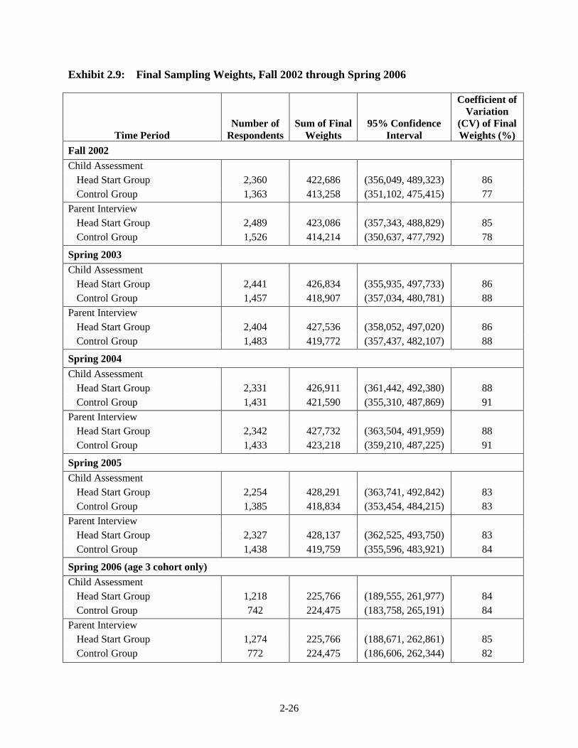
Interview (PI) by Child and Program Characteristics ....................................... 2-21 2.9 Final Sampling Weights, Fall 2002 through Spring 2006 ................................ 2-26 2.10 Unweighted and Weighted Cross-Sectional Response Rates by Wave ............ 2-27 2.11 Unweighted and Weighted Response Rates by Wave for Teacher
Survey/Teacher Child Report (TS/TCR), Classroom Observation, and Director Interview, Conditional on Child Assessment and Parent Interview Response ........................................................................................... 2-29
2.12 Variables Correlated with Teacher Survey (TS), Teacher Child Report
(TCR), Classroom Observation (CO), and Center Director Interview (DI) Nonresponse .............................................................................................. 2-30
2.13 Unweighted Response Rates for Teacher Survey (TS), Teacher Child
Report (TCR), Classroom Observation (CO) and Center Director Interview (DI), Conditional on Child Assessment and Parent Interview Respondents ..................................................................................................... 2-31
2.14 Unweighted Longitudinal Response Rates ...................................................... 2-35 3.1 Direct Child Assessment Measures by Cohort and Year for the
Combined Sample ............................................................................................. 3-4 3.2 Direct Child Assessment Measures by Cohort and Year for the Spanish
Sample in Puerto Rico ...................................................................................... 3-5 3.3 Item Response Curve for TVIP Item # 8: A Multiple-Choice Item
Scored Right/Wrong ........................................................................................ 3-13 3.4 IRT True-Score for the 32-Item TVIP Kindergarten Test ................................ 3-14

iv
Contents (continued)
Exhibits (continued) Page 3.5 Illustration of Test Characteristic Curves of a Test Administered to Two
Different Samples ............................................................................................. 3-15 3.6 Test Characteristic Curves of a Test Administered to Two Different
Samples, After Equating ................................................................................... 3-15 3.7 PPVT Version Used by Cohort and Data Collection Wave ............................. 3-17 3.8 Composite Measures by Cohort and Year for the Combined Sample .............. 3-23 3.9 Percentiles on the Norm-Referenced Tests for the 4-Year-Old Cohort by
Year ................................................................................................................... 3-24 3.10 Percentiles on the Norm-Referenced Tests for the 3-Year-Old Cohort by
Year ................................................................................................................... 3-25 3.11 Fall 2002 Psychometric Data for All Outcomes by Cohort .............................. 3-31
3.12 Spring 2003 Psychometric Data for All Outcomes by Cohort ......................... 3-33 3.13 Spring 2004 Psychometric Data for All Outcomes by Cohort ......................... 3-35 3.14 Spring 2005 Psychometric Data for All Outcomes by Cohort ......................... 3-38 3.15 Spring 2006 Psychometric Data for All Measures by Cohort .......................... 3-41 3.16 Components of Variance and ICC's by Cohort for Fall 2002 ........................... 3-44 3.17 Components of Variance and ICC's by Cohort for Spring 2003 ...................... 3-46 3.18 Components of Variance and ICC's by Cohort for Spring 2004 ...................... 3-48 3.19 Components of Variance and ICC's by Cohort for Spring 2005 ...................... 3-50 3.20 Components of Variance and ICC's by Cohort for Spring 2006 ...................... 3-53 4-1 Data Collection Schedule – 3-Year-Old Cohort ............................................... 4-2 4-2 Data Collection Schedule – 4-Year-Old Cohort ............................................... 4-2 5.1 Summary of the HSIS Measures by Domain and Data Collection Period ....... 5-2

v
Contents (continued)
Exhibits (continued) Page 5.2 Demographic and Time Variables Included in the Statistical Models
Estimating the Impact of Head Start ................................................................. 5-6 5.3 Percent of Treatment and Control Children Assessed by Month of
Assessment........................................................................................................ 5-7 5.4 Measures of Fall 2002 “Starting Points” Used in the Regression Models,
by Child and Parent Outcomes ........................................................................ 5-10 5.5 Item Nonresponse Rates for Fall 2002 Imputed Variables Used in the
Analysis ............................................................................................................ 5-15 5.6 Number of Respondents by Wave and Age Cohort .......................................... 5-22 5.7 Distribution of Start Dates for Crossovers and Treatment Group
Participants........................................................................................................ 5-49 5.8 IOT Sensitivity Analysis for the 3-Year-Old Cohort ....................................... 5-52 5.9 IOT Sensitivity Analysis for the 4-Year-Old Cohort ....................................... 5-52 5.10 Variables Used To Define Subgroups, Measured At Baseline ......................... 5-56 5.11 Agreement between Race of Child and Biological Mother/Caregiver,
and between Child Testing Language and Home Language ............................ 5-57 5.12 Distribution of the Pre-Academic Standard Cluster W-ability Scores for
the English-English Group, Fall 2002 .............................................................. 5-58 5.13 Distribution of the Pre-Academic Standard Cluster W-ability Scores for
the Spanish-English Group, Fall 2002 .............................................................. 5-58

1-1
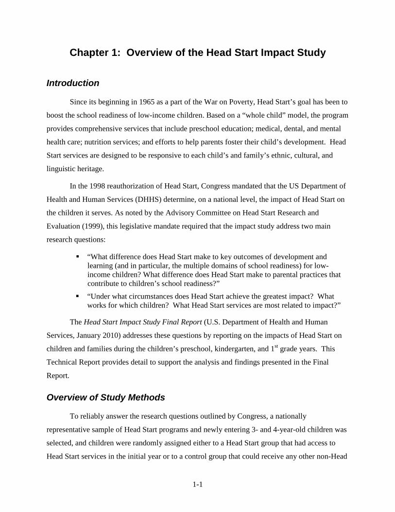
Chapter 1: Overview of the Head Start Impact Study
Introduction
Since its beginning in 1965 as a part of the War on Poverty, Head Start’s goal has been to
boost the school readiness of low-income children. Based on a “whole child” model, the program
provides comprehensive services that include preschool education; medical, dental, and mental
health care; nutrition services; and efforts to help parents foster their child’s development. Head
Start services are designed to be responsive to each child’s and family’s ethnic, cultural, and
linguistic heritage.
In the 1998 reauthorization of Head Start, Congress mandated that the US Department of
Health and Human Services (DHHS) determine, on a national level, the impact of Head Start on
the children it serves. As noted by the Advisory Committee on Head Start Research and
Evaluation (1999), this legislative mandate required that the impact study address two main
research questions:
“What difference does Head Start make to key outcomes of development and learning (and in particular, the multiple domains of school readiness) for low-income children? What difference does Head Start make to parental practices that contribute to children’s school readiness?”
“Under what circumstances does Head Start achieve the greatest impact? What works for which children? What Head Start services are most related to impact?”
The Head Start Impact Study Final Report (U.S. Department of Health and Human
Services, January 2010) addresses these questions by reporting on the impacts of Head Start on
children and families during the children’s preschool, kindergarten, and 1st grade years. This
Technical Report provides detail to support the analysis and findings presented in the Final
Report.
Overview of Study Methods
To reliably answer the research questions outlined by Congress, a nationally
representative sample of Head Start programs and newly entering 3- and 4-year-old children was
selected, and children were randomly assigned either to a Head Start group that had access to
Head Start services in the initial year or to a control group that could receive any other non-Head
1-2
Start services available in the community, chosen by their parents. In fact, approximately 60
percent of control group parents enrolled their children in some other type of preschool program
in the first year. In addition, all children in the 3-year-old cohort could receive Head Start
services in the second year. Under this randomized design, a simple comparison of outcomes for
the two groups yields an unbiased estimate of the impact of access to Head Start in the initial
year on children’s school readiness. This research design, when properly implemented, would
ensure that the two groups did not differ in any systematic or unmeasured way except through
their access to Head Start services. It is important to note that, because the control group in the
3-year-old cohort was given access to Head Start in the second year, the findings for this age
group reflect the added benefit of providing access to Head Start at age three, not the total benefit
of having access to Head Start for two years.
In addition to random assignment, this study is set apart from most program evaluations
because it includes a nationally representative sample of programs, making results generalizable
to the Head Start program as a whole, not just to the selected samples of programs and children.
However, the study does not represent Head Start programs serving special populations, such as
tribal Head Start programs, programs serving migrant and seasonal farm workers and their
families, or Early Head Start. Further, the study does not represent the 15 percent of Head Start
programs in which the shortage of Head Start slots was too small to allow for an adequate
control group.
Selected Head Start grantees and centers had to have a sufficient number of applicants for
the 2002-03 program year to allow for the creation of a control group without requiring Head
Start slots to go unfilled. As a consequence, the study was conducted in communities that had
more children eligible for Head Start than could be served with the existing number of funded
slots.
At each of the selected Head Start centers, program staff provided information about the
study to parents at the time enrollment applications were distributed. Parents were told that
enrollment procedures would be different for the 2002-03 Head Start year and that some
decisions regarding enrollment would be made using a lottery-like process. Local agency staff
implemented their typical process of reviewing enrollment applications and screening children
1-3
for admission to Head Start based on criteria approved by their respective Policy Councils. No
changes were made to these locally established ranking criteria.
Information was collected on all children determined to be eligible for enrollment in fall
2002, and an average sample of 27 children per center was selected from this pool: 16 who were
assigned to the Head Start group and 11 who were assigned to the control group. Random
assignment was done separately for two study samples—newly entering 3-year-olds (to be
studied through two years of Head Start participation i.e., Head Start year and age 4 year,
kindergarten, and 1st grade) and newly entering 4-year-olds (to be studied through one year of
Head Start participation, kindergarten, and 1st grade).
The total sample, spread over 23 different states, consisted of 84 randomly selected Head
Start grantees/delegate agencies, 383 randomly selected Head Start centers, and a total of 4,667
newly entering children, including 2,559 in the 3-year-old group and 2,108 in the 4-year-old
group.1
Data collection began in the fall of 2002 and continued through the spring of 2006,
following children from entry into Head Start through the end of 1st grade. Comparable data
were collected for both Head Start and control group children, including interviews with parents,
direct child assessments, surveys of Head Start and non-Head Start teachers, interviews with
center directors and other care providers, direct observations of the quality of various care
settings, and care provider assessments of children. Response rates were consistently quite high,
approximately 80 percent for parents and children throughout the study.
Although every effort was made to ensure complete compliance with random assignment,
some children accepted into Head Start did not participate in the program (about 15 percent for
the 3-year-old cohort and 20 percent for the 4-year-old cohort), and some children assigned to
the non-Head Start group nevertheless entered the program in the first year (about 17 percent for
3-year-olds and 14 percent for 4-year-olds), typically at centers that were not in the study
sample. These families are referred to as “no shows” and “crossovers.” Statistical procedures
for dealing with these events are discussed in this report and the Final Report. The study
1 The sample of 3-year-olds is slightly larger than the sample of 4-year-olds to ensure that an adequate sample size
was maintained, given the possibility of higher study attrition resulting from an additional year of longitudinal data collection for the younger children.

1-4
findings provide estimates of both the impact of access to Head Start using the sample of all
randomly assigned children and the impact of actual Head Start participation (adjusting for the
no shows and crossovers) as well as subgroup impact estimates.
Contents of Report
This Technical Report is designed to provide technical detail to support the analysis and
findings presented in the Head Start Impact Study Final Report (U.S. Department of Health and
Human Services, January 2010). Chapter 1 provides an overview of the Head Start Impact Study
and its findings. Chapter 2 provides technical information on the analytical sampling weights
used in the analysis. A description of the outcome measures and their psychometric properties is
provided in Chapter 3 and the description of the data collection procedures is provided in
Chapter 4. Chapter 5 provides a description of the impact analysis methods including ITT
(intent-to-treat) impact estimates, IOT (impact on the treated) impact estimates, and subgroup
impact estimates.
1-5
References
Advisory Committee on Head Start Research and Evaluation (1999). Evaluating Head Start: A Recommended Framework for Studying the Impact of the Head Start Program. Washington, DC: US Department of Health and Human Services.
U.S. Department of Health and Human Services, Administration for Children and Families. (January 2010). Head Start Impact Study. Final Report. Washington, DC: Author.

2-1
Chapter 2: Analytical Sampling Weights
Overview
Sampling weights were calculated for each child to allow estimates based on the sample
to represent the national population of newly entering Head Start participants for 2002. Because
children were randomly assigned to Head Start (i.e., the “program or Head Start” group) and
non-Head Start (i.e., the “control” group) groups within each Head Start center, the two groups
represents the same Head Start population of newly entering children when appropriately
weighted. The only difference, theoretically, is that the Head Start group was allowed access to
attend Head Start at the time of random assignment, while the control group was not.
Each study child was assigned a base weight that reflected his/her overall probability of
selection, including the sampling of broad geographic areas used as primary sampling units
(PSUs), Head Start grantees/delegate agencies, and centers (see below). These base weights
were then adjusted for nonresponse to the child assessment and parent interview at each wave of
data collection, to produce separate fall 2002, spring 2003, spring 2004, spring 2005, and spring
2006 weights.2
These cross-sectional child weights are used for most analyses in this report; the analyses
focus on impacts at different time points and include only children and families for whom spring
data are available. Fall 2002 weights are used to examine distributions of child and family
characteristics at the beginning of the analysis period, in fall 2002. Two sets of longitudinal
child weights were also created for use in fitting growth curves. The first set applies to children
The nonresponse-adjusted weights of children in the 4-year-old group were
poststratified to the Head Start National Reporting System (HSNRS) newly entering enrollment
totals for 4-year-olds (comparable totals for 3-year-olds were not available). Extremely large
weights were then trimmed for both age groups. The final child and parent weights are the
product of the overall base weight, a nonresponse adjustment factor, a poststratification factor,
and a trimming factor. For variance estimation, a set of 76 jackknife replicate weights was
created for each child.
2 The 4-year-olds do not have spring 2006 weights because they were in second grade in 2006 and not included in
this wave of data collection.

2-2
with assessments at two or more time points, and the second set applies to children with three or
more assessments in the fall 2002 to spring 2006 data collection period.
Primary Sampling Unit (PSU) Weights
The frame of 161 PSUs, or geographic clusters, covering all Head Start grantees in the
U.S. and Puerto Rico was classified into 25 approximately equal-sized strata based on the
following: 1) the level of services for low-income preschool children in the state; 2) the
percentage of minority Head Start enrollment in the PSU; 3) the Head Start region; and 4) the
percentage of Head Start enrollment in an MSA (a U.S. Census Bureau metropolitan statistical
area). One PSU in each stratum was sampled with probability proportional to the total Head
Start enrollment of 3- and 4-year-olds in the PSU. The source of enrollment was the 1999-2000
Head Start Program Information Report (PIR). The PSU weight is the inverse of the PSU
probability of selection:
PSU weight = (Total Age 3 & 4 Enrollment in Stratum h) / (Total Age 3 & 4 Enrollment in PSU) where h = 1, 2, ….25.
There was one certainty PSU whose probability of selection was 1 due to its large Head Start
enrollment.
Head Start Program Weights
Program Sampling
There were two stages of sampling within most PSUs, and three stages within three
extremely large PSUs. Prior to sampling, small programs were collapsed into groups consisting
of two to four programs. These were sampled as a unit; thus, the within-PSU probability of
selection for each program in a given group is the same.
Prior to telephone screening, programs and program groups (referred to henceforth
simply as program groups,3
3 Note that most “program groups” consisted of a single grantee or delegate agency.
) were sampled within the three large PSUs to reduce screening costs.
In each of these three PSUs, 12 program groups were sampled with probability proportional to
total age three and four enrollment from the 1999-2000 PIR and only these program groups were
screened. With this one exception, all programs in the sample PSUs underwent screening,

2-3
during which study staff collected information on additional characteristics of each program and
its community. A major purpose of this screening was to identify situations in which Head Start
“saturated” the community, that is, where the local program was large enough that all of the
interested and eligible families in the community could be enrolled, making selection of a non-
Head Start study group impossible without simultaneously leaving some of the program’s
capacity unused. After screening, program groups were sampled within the 25 PSUs from
among those determined to be neither saturated nor closed. Within each PSU, four program
groups were sampled with probability proportional to the total newly entering children ages three
and four enrollment. From these, three program groups were subsampled with equal
probabilities to be the main sample, and the remaining program group was assigned as a reserve
sample. The main sample consisted of 76 program groups (in one PSU, all four program groups
were sampled with certainty into the main sample) which comprised 90 individual programs.
The reserve sample consisted of 30 programs.
Program Base Weights, Adjustments for Saturation, Raking
Each of the 90 programs in the main sample received a base weight. The program base
weight was the inverse of the overall probability of selection for that program, including the PSU
probability of selection and the sampling of program groups within the PSU.
The base weights were adjusted for undercoverage due to the deletion from the frame of
eight Head Start programs involved in the most recent FACES study (in order to minimize
burden on these programs) and 28 programs discovered to be saturated during the screening.
Because these programs had no chance of selection, an undercoverage adjustment was needed to
correct for bias, in case the deleted programs were systematically different from those retained
on the frame (see discussion below) and to prevent weighted enrollment totals from the sample
from being too low. The undercoverage adjustment factor was calculated as the ratio of the
estimated total newly entering enrollment (including saturated programs) in the PSU to the
estimated newly entering enrollment from the sampled programs in the PSU, using enrollment
information collected during the telephone screening. This adjustment corrected for differences
between saturated and non-saturated programs on broad geographic factors and size in terms of
enrollment, but not for other types of differences between the two types of programs within
2-4
PSUs—differences that could result in larger or smaller Head Start impacts in the studied sites
than in the nation as a whole.
Additionally, the adjusted program weights for all 90 main sample programs were then
raked using marginal ages three and four enrollment totals from the 1999-2000 PIR. The raking
dimensions were urban status (central city, noncentral city, rural), Head Start region (Northeast,
North Central, South, Plains, West), and level of pre-K services in the state (state has Head Start-
like programs, state has other types of programs, state has no programs). This procedure served
to further match the analysis sample to the full national Head Start program frame on these
factors. Since the number of sampled programs in each cross-classification was generally small,
raking, or iterative proportional fitting, rather than poststratification, was used (Oh & Scheuren,
1987). In raking, the weights are consecutively ratio-adjusted to marginal totals, typically from
an external data source, until the resulting weighted totals converge to the totals for each
dimension. The adjustment factor at each iteration is the ratio of the PIR total for the marginal
dimension to the sample estimate of the same total, where the weight in the sample estimate is
the program weight from the previous raking iteration. This ratio adjustment reduces the
sampling error associated with the sampling of PSUs and programs for estimates of Head Start
children by urban status and Head Start region (Cochran, 1977). However, it is not intended to
result in sample estimates that will agree with external totals of newly enrolled Head Start
children, since no such counts exist.
After these undercoverage and raking adjustments were performed, the program weights
in two PSUs were further adjusted to compensate for dropping two eligible programs from the
sample because of their participation in another Head Start study, the Quality Research
Consortium (QRC) and for dropping three programs because they were found to be saturated
after sampling. Another program was discovered to have closed, reducing the number of
participating programs to 84. The adjustment factor was calculated as the ratio of estimated total
newly entering enrollment in the PSU based on the sample of programs in the PSU (excluding
one program that had closed) to the weighted newly entering enrollment for the sampled
nonsaturated, non-QRC programs in the PSU. None of the programs refused to participate, thus
no nonresponse adjustment or reserve programs were needed.

2-5
Final Program Weight
Eighty-four programs received a final program weight. The final program weight can be
written as:
Final program weight = PSU weight x (1/ P1) x (1/ (1-PFACES)) x (1/ P2) x (1/ P3) x FSat1 x FRK x FQRC, Sat2
where,
PFACES = probability of selection in FACES, P1 = probability of being subsampled prior to telephone screening in three large PSUs, P2 = probability of being sampled in PSU, P3 = probability of being subsampled for main sample, FSat1 = adjustment factor for dropping 28 saturated programs from frame before sampling, FRK = raking adjustment factor to reduce sampling error, FQRC, Sat2 = adjustment factor for dropping two programs participating in QRC and three
saturated programs from the sample,
where,
P1 = 12*(Total Age 3 & 4 Enrollment in Program Total Age 3 & 4 Enrollment in PSU), P2 = 4*(1st Yr Age 3 & 4 Enrollment in Program 1st Yr Age 3 & 4 Enrollment in PSU),
∑
∑
=
+
== n
1ii
mn
1ii
Sat1
i Programin Enrollment 3,4 Age EnteringNewly
i Programin Enrollment 3,4 Age EnteringNewly
*w
*wF where n is the number of
eligible (nonsaturated) sampled programs in the PSU and m is the number of saturated programs
in the PSU that were excluded from sampling. For the n programs, wi is the program weight that
reflects all stages of sampling through P3. For the m saturated programs, wi reflects all stages of
sampling through P1 (note P1=1 except in three very large PSUs, where subsampling was done to
reduce the burden of telephone screening).
∑
∑−
=
== mn
1ii
n
1ii
Sat2 QRC,
i Programin Enrollment 3,4 Age EnteringNewly
i Programin Enrollment 3,4 Age EnteringNewly
*w
*wF where wi is the program weight
reflecting all stages of sampling, the FSat1 adjustment, and the raking; n is the number of sampled
programs in the PSU (excluding one program that had closed), and m is the number of QRC and
saturated programs discovered in the sample in the PSU.

2-6
The final program weights for the sample of 84 programs sum to 1,216 with a 95% confidence
interval of [959, 1,472].
Head Start Centers
Center Sampling
Within each program, a list of the centers was obtained, and the centers were screened
using a Center Information Form (CIF) to collect various statistical data. In addition to screening
for saturation at the program level, any centers that were determined to be saturated were
dropped from the frame in each program.4
Center Base Weights and Adjustments for Saturation and Nonresponse
Prior to sampling, small centers were combined into
groups that ranged from two to eight centers and were treated as a unit for sampling purposes.
Therefore, each center in a given group had the same probability of selection, namely that of the
group. An initial sample of center groups was selected with probability proportional to newly
entering age three and four enrollment in the center group. The initial sample of center groups
was then subsampled with equal probabilities. The subsample was retained as the main sample
in each program, while the remaining center groups formed a reserve sample. In general, three
center groups per program (or program group) were selected for the main sample and two for the
reserve. However, in very large programs four to six center groups were allocated for the main
sample and three for the reserve. Within a program group, the total number of centers was
allocated proportionally to the programs based on their newly entering enrollments. A total of
221 center groups (consisting of 448 individual centers) were selected for the main sample, and
114 center groups (consisting of 237 individual centers) were selected for the reserve sample.
The center base weight was calculated as the inverse of the overall probability of
selection for each center, including the sampling of PSUs, programs, and centers within
programs. The center base weights were adjusted for deleting 154 saturated centers and 2
centers participating in a QRC study from the frame prior to center sampling. These adjusted
weights were further adjusted for the refusal of five sampled centers to participate in the study,
4 Hence a center might be excluded from sampling due to saturation, even if the grantee or delegate agency running
that center was included in the study (and other centers in that same program or delegate agency were eligible for sampling).

2-7
and for the loss of 56 centers discovered to be saturated after sampling. In these centers, no
sampling of children was possible. In addition, six centers had closed, and 13 were ineligible for
other reasons, such as merging with another center. For the merged centers, where appropriate,
an adjustment was made to the base weight of the newly merged center to account for its
increased probability of selection, since the individual centers had been listed separately on the
center frame.
The adjustment factor for dropping saturated centers from the frame was calculated as the
ratio of the estimated total newly entering enrollment (including from saturated centers) in the
program to the newly entering enrollment estimated from the sampled centers in the program.
The newly entering enrollment was collected on the CIF during center screening and updated
during October through December 2002 for all centers where possible. The adjustment factor
was calculated separately for each program, unless this resulted in a very large adjustment, in
which case the factor was calculated for the PSU.
The adjustment factor for the loss of five refusing and 56 saturated centers was calculated
as the ratio of the weighted newly entering enrollment for the entire center sample in the program
(excluding those that had closed or merged) to the weighted newly entering enrollment for the
nonsaturated, cooperating sampled centers in the program. Overall, these procedures adjusted
for size differences between included and excluded centers, but not for other center differences
that could lead to different-sized impact estimates.
Final Center Weight
The final center weight can be written as:
Final Center Weight= Final Program Weight x (1/Pc1) x (1/Pc2) x FQRC x FSat1 x FRefusal, Sat2,
where,
PC1 = probability of selection for initial center sample (both main and reserve), PC2 = probability of selection for main center sample, FQRC = adjustment factor for dropping two centers participating in QRC from frame, FSat1 = adjustment factor for dropping 154 saturated centers from frame, FRefusal, Sat2= adjustment factor for dropping 56 saturated centers and 5 refusing centers from
sample,

2-8
PC1= RMCenters)/n edNonsaturat Eligible,for Programin Enrollment 4&3 Age Entering(Newly
GroupCenter in Enrollment 4&3 Age EnteringNewly
+
,
PC2= Program the in Reserve Main,Both for SampledGroups Center#
Program the in Sample Mainfor d SubsampleGroups Center#nn
RM
M =+
,
Centers) QRC 2in Enrollment Entering(Newly -Program)in Enrollment 3,4 Age Entering(Newly Programin Enrollment 3,4 Age EnteringNewly
QRCF =
Note that FQRC = 1.25103 for centers in the one program that contained the two QRC centers and
is equal to one for centers in all remaining programs.
∑
∑
=
+
== n
1ii
mn
1ii
1Sat
iCenterin Enrollment 3,4 Age EnteringNewly
iCenterin Enrollment 3,4 Age EnteringNewly
*w
*wF
where n is the number of sampled centers in the program, m is the number of saturated centers
on the frame in the program that were excluded from sampling, wi is the center weight through
the FQRC adjustment for sampled centers, and wi is the final program weight for saturated centers
excluded from the frame in the program prior to center sampling.
∑
∑−
=
== mn
1ii
n
1ii
2Sat,refusal
iCenterin Enrollment 3,4 Age EnteringNewly
iCenterin Enrollment 3,4 Age EnteringNewly
*w
*wF
where n is the number of sampled centers in the program, m is the number of refusing and
saturated centers discovered among those sampled in the program, and wi is the center weight
through the Fsat1 adjustment.
The final center weight reflects the PSU and program probabilities of selection. In four
programs, all reserve centers were brought into the sample when the original centers were found
to be saturated or partially saturated and hence unable to provide the planned number of control
group children. In these centers, PC2 was set to one in the above formula. When this resulted in a
census of eligible centers in the program, both Pc1 and Pc2 were set to one. In six programs where
some, but not all, of the reserve centers were activated to offset saturation in the main sample, n
M includes the reserves that were activated as well as the main sample centers. In this situation,
2-9
centers were randomly subsampled from among the reserve centers selected for that particular
program or program group. The total number of centers in the final sample, including main
sample and activated reserves was 458. The sample was reduced to 378 after losing 19 centers
identified following selection as ineligible (closings, mergers), five identified as noncooperating,
and 56 found to be saturated.
Reserve centers were picked at random from the same pool as the main sample centers,
from the same program where possible, but with no other attempt to match them with the
characteristics of the centers they were replacing. The purpose of the reserve sample was
primarily to prevent a sample size shortfall due to loss of centers, rather than to reduce the bias
caused by exclusion of saturated and refusing centers from the study. The weighting adjustments
to the center weights were designed to accomplish the latter.
The final center weights for the 378 centers sum to 12,705 with a 95% confidence
interval of [10,290, 15,119].
Comparison of Head Start Grantees/Delegate Agencies and Centers in Saturated and Non-Saturated Communities
As discussed in Chapter 2, there is potential for undercoverage bias due to the exclusion
from the sampling frame of Head Start grantees/delegate agencies and centers in communities
saturated by the program, that is, communities with too few families who are able, eligible or
interested in accessing Head Start (beyond those the program can accommodate) to provide a
randomly selected control group for the study. Newly entering Head Start children in these
saturated communities had no chance of selection and therefore are not represented by our
sample. Consequently, the potential for bias arises if the saturated grantees/delegate agencies
and centers are systematically different from the non-saturated grantees/delegate agencies and
centers we retained in the sampling frame and if the characteristics on which they differ are
correlated with the outcome measures for and impact estimates on the children they enroll.
However, if the children in these excluded grantees/delegate agencies and centers represent only
a small percentage of the Head Start population, then the potential for bias is much less. Based
on the sample coverage rate reported in Chapter 2 of the Final Report, 15.5 percent of the
children served by Head Start nationally are omitted from the study. This noncoverage rate is
based on grantees and centers identified in the sample frame and samples that were excluded due

2-10
to saturation. It equals 1 minus the product of four coverage rates: program frame x program
sample x center frame x center sample. Mathematically, this equates to 1-(0.962 x 0.975 x
0.952 x 0.947) = 1-0.845 = 0.155.
Head Start Grantees/Delegate Agencies
Exhibits 2.1 and 2.2 compare saturated and non-saturated grantees/delegate agencies by a
few characteristics available on the Head Start Program Information Report (PIR) database (and,
for newly entering enrollment and additional center information, telephone screening
confirmation calls to grantees and delegate agencies prior to sampling). The grantees/delegate
agencies were weighted to account for sampling of broad geographic areas (i.e., PSUs) and for
the subsampling of grantees/delegate agencies in three large urban cities prior to the telephone
screening (see Chapter 2 of the Final Report). This was necessary to draw conclusions about the
entire population of children served by Head Start and not merely the children served by
grantees/delegate agencies in the 25 sampled PSUs that were screened to determine saturation.
Tests of statistical significance were performed to reduce the possibility of drawing false
conclusions from differences that may have been due to sampling error. The hypothesis testing
was done in WesVar using jackknife replicate weights to account for the study’s complex sample
design. Exhibit 2.1: Comparison of Saturated and Non-Saturated Head Start Grantees/Delegate
Agencies by Enrollment
Enrollment Variable Saturated Programs
Non-Saturated Programs
P-Value (t-Test of
Difference) Percent Hispanic Enrollment 9% 26% 0.001 Percent Black Enrollment 20% 33% 0.134 Age 3 Enrollment as Percent of Total Enrollment 52% 49% 0.535 Average Total Enrollment 188 571 <0.001 Average Newly Entering Enrollment 113 388 <0.001

2-11
Exhibit 2.2: Comparison of Saturated and Non-Saturated Head Start Grantees/Delegate Agencies by Location Characteristics
Characteristics Saturated Programs
Non-Saturated Programs
p-Value (Chi-Square Test of
Association) School-based 0.018
Yes 66% 21% No 34% 79%
Metro Status 0.91 MSA 66% 68% Non-MSA 34% 32%
Level of Pre-K Services in State 0.60 Similar to Head Start 35% 25% Some Head Start-Like 27% 20% Remaining States 38% 55%
Head Start Region 0.15 Northeast 24% 25% North Central 48% 24% South 28% 39% Plains 0% 4% West 0% 8%
As shown in these tables, the saturated grantees/delegate agencies are much smaller,
much more likely to be school-based, and have smaller percentages of Hispanic enrollment than
the non-saturated grantees/delegate agencies. Although they appear to be more often located in
the Midwest, differences in the distribution of saturated vs. non-saturated grantees/delegate
agencies by Head Start regions are not statistically significant. A cautionary note is that
variances at the program level are not very stable because the number of saturated
grantees/delegate agencies is small. In addition, variances do not include the between-PSU
component of variance due to sampling PSUs; thus, they are underestimates, and the p-values
may be slightly overstating the significance of the differences.
Head Start Centers
Exhibits 2.3 and 2.4 compare saturated and non-saturated centers by various qualitative
characteristics and enrollment variables available from the CIFs completed by all centers in the
sampled grantees and delegate agencies. All hypothesis testing was again done in WesVar using
jackknife replicate weights to account for the study sample design. The replicate weights do not
include the between-PSU variance component; therefore, the p-values in these tables may
2-12
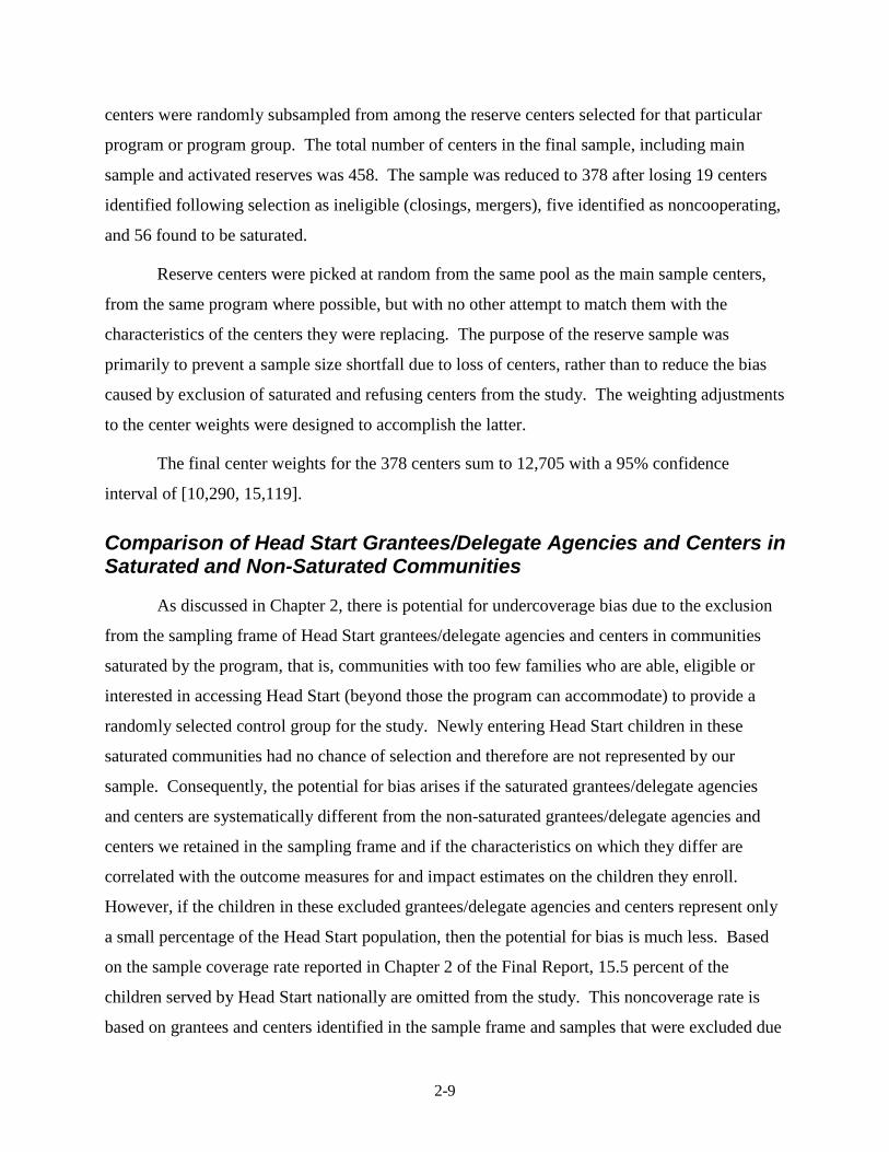
slightly overstate the significance of the difference. In Exhibit 2.3, the chi-square test was not
able to detect a significant difference for type of program option offered, whether staff members
are school employees, metro status, region, or level of Pre-K services available in the state. With
respect to enrollment, Exhibit 2.4 shows that the saturated centers are smaller, have fewer
Hispanic children, and have a larger percentage of first-year 3-year-olds than the non-saturated
centers. As expected, these centers do not have waiting lists, a significant difference from non-
saturated centers.
Exhibit 2.3: Comparison of Saturated and Non-Saturated Head Start Centers Operated
by Non-Saturated Programs, by Program and Location Characteristics
Characteristics Saturated Centers
Non-Saturated Centers
p-Value (Chi-Square Test of
Association) Program Option 0.44
Full-Day Only 35% 28% Part-Day Only 52% 50% Other 13% 22%
Staff Are School Employees 0.249 Yes 17% 11% No 83% 89%
Metro Status 0.64 MSA 74% 70% Non-MSA 26% 30%
Head Start Region 0.376 Northeast 32% 27% North Central 34% 20% South 17% 31% Plains 12% 11% West 4% 11%
Level of Pre-K Services in State 0.212 Similar to Head Start 40% 22% Some Head Start-Like 15% 18% Remaining States 45% 60%

2-13
Exhibit 2.4: Comparison of Saturated and Non-Saturated Head Start Centers Operated by Non-Saturated Programs, by Enrollment
Enrollment Characteristic Saturated Centers
Non-Saturated Centers
p-Value (t-test of Difference)
Percent Hispanic Enrollment 17% 30% 0.005 Percent Black Enrollment 38% 26% 0.204 Percent Newly Entering Enrollment 65% 66% 0.985 Age 3 Enrollment as Percent of Newly Entering
Enrollment 54% 47% 0.037 Number of Children on Waiting List as Percent of
Total Enrollment 0% 15% <0.001 Average Number Funded Slots 37 48 0.036 Average Total Enrollment 26 47 <0.001 Average Newly Entering Enrollment 16 31 <0.001 Average Number on Waiting List 0 9 <0.001
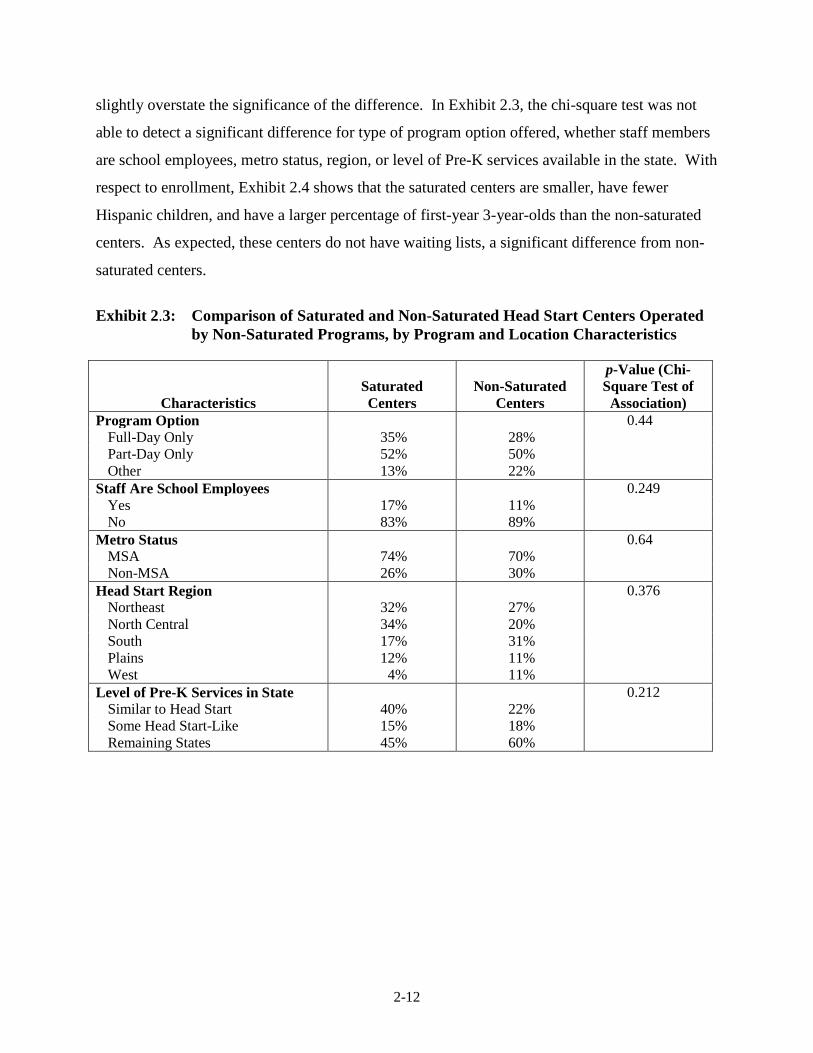
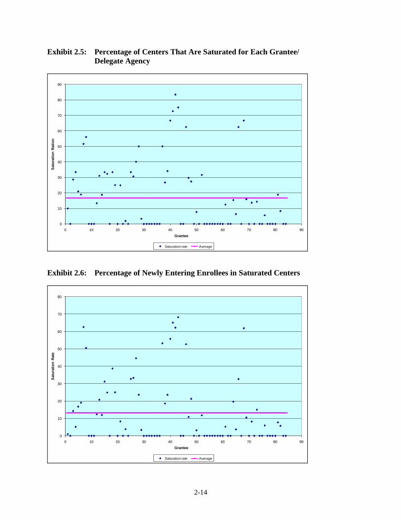
Two graphs follow Exhibit 2.4 that show the percentage of centers that are saturated for
each of the 84 grantees/delegate agencies with less than 100 percent saturation rate. The
saturation rate was calculated two ways: as the percentage of centers in each program that are
saturated (Exhibit 2.5) and as the percentage of newly entering enrollment in saturated centers
for each program (Exhibit 2.6). The average percentage of saturated centers is 16.6 percent,
while the average percentage of newly entering enrollment in saturated centers is 13.2 percent,
another indication that the saturated centers tend to be smaller. The graphs show the variation
among grantees/delegate agencies in the share of centers operating in saturated communities and
the share of newly entering children served by those centers.
2-14
Exhibit 2.5: Percentage of Centers That Are Saturated for Each Grantee/ Delegate Agency
0
10
20
30
40
50
60
70
80
90
0 10 20 30 40 50 60 70 80 90
Satu
ratio
n Ra
tion
Grantee
Saturation rate Average Exhibit 2.6: Percentage of Newly Entering Enrollees in Saturated Centers
0
10
20
30
40
50
60
70
80
0 10 20 30 40 50 60 70 80 90
Satu
ratio
n Ra
te
Grantee
Saturation rate Average
2-15
Child Weights
Random Assignment of Children Within Centers
The random assignment of children, that is, the sampling of children into the Head Start
and control groups, began with the acquisition of information on every applicant for the 2002-03
program year and the number of available slots in the center. Eligible returning children (who
were not subject to random assignment) were allowed to attend Head Start. The remaining
eligible newly entering children on the center’s applicant list were then sorted based on child
need (using local program criteria), as they normally would be to determine which children to
admit and which to put on a waiting list, and the list was truncated at exactly the number of
children needed to both fill the center’s remaining slots and supply a non-Head Start group
sample of the desired size for the study. A sample of children was randomly selected with equal
probabilities from the truncated list to fill the center’s slots. Those not selected to fill a slot from
the truncated list were assigned to the control group. The children sampled to fill the center’s
slots were then subsampled to obtain the targeted number of Head Start group children. This
resulted in three categories of children: (1) those sampled to attend the Head Start program who
would not be included in the study, (2) those sampled for the study’s Head Start group, and
(3) those sampled for the study’s control group. All remaining applicants (including those
coming in during the year) were put on the waiting list; these children had no chance of selection
for either study sample but could enter the Head Start program later (once sampling ended) to
replace children who dropped out of the program over the course of a year. The targeted number
of Head Start and control group children was 16 and 11, respectively, at most centers and center
groups, cumulating to an average of 48 Head Start group members and 32 control group cases
for each sampled program group. This uneven balance only slightly reduces the statistical
precision of the impact estimates and hence the probability of detecting as statistically significant
any impact that does occur compared to a perfectly balanced design;5
5 Standard errors of impact estimates and minimum detectable effect sizes increase by about two percent.
its advantage is in reducing
the number of control group children excluded from the program at each center or center group.
In center groups, the 16 Head Start group children and 11 control group children were
proportionally allocated to the centers in the group based on newly entering enrollment. In three
of the 84 programs, children applied directly to the program rather than the center, so it was
2-16
necessary to randomly assign children at the program level and sample 48 Head Start group and
32 control group cases to obtain 80 children for the program in total. The total target sample size
was approximately 3,600 Head Start group children and 2,400 control group children.
The random assignment of children was spread out over the spring/summer 2002,
because most centers took applicants on a flow basis and preferred to let their families know
soon whether their child had been accepted to attend the Head Start program. This meant
children were sampled in batches or rounds, and the sampling process described above took
place more than once in most centers. An additional complication was that stratification by
program option (e.g., part- vs. full-time) was used in many centers. The allocation of the total
number of Head Start and control group children across program options and rounds at each
center was approximately proportional to the newly entering enrollment in each program option
and the number of slots filled in each round. The actual probabilities of selection for each child
were stored electronically for weighting purposes. However, the probabilities can vary greatly
because of the difficulty in allocating across rounds. There were many rounds where children
were sampled to fill slots but no Head Start or control group children were selected because the
target sample sizes of Head Start and control group children had already been obtained. None of
these children had a chance of selection for the study, meaning child weights based on the actual
probabilities of selection would underestimate the size of the first-year Head Start population.
Therefore, the within-center child probabilities of selection were calculated as a simple sampling
fraction: the number of children sampled in the center divided by the newly entering fall 2002
age 3 & 4 enrollment in the center.
Child Base Weights
The within-center child base weight was calculated as:
Center in SampledChildren StartHead #Center in Enrollment 4&3 Age EnteringNewly
for the sampled Head Start group children, and as
Center in SampledChildren Groups Control#Center in Enrollment 4&3 Age EnteringNewly
2-17
for the control group children. Note that the numerator is the same for both groups, since
estimates are to be made for the universe of newly entering Head Start children using either
sample. For centers where the updated fall 2002 newly entering enrollment was not obtained,
the newly entering enrollment figure for the previous program year was used. When this was
missing, and for three programs where children were randomly assigned at the program level
rather than at the center level, the inverse of the actual probability of selection for children in the
center was used as the base weight.
The overall child base weight reflecting all stages of sampling can be written as:
Overall Child Base Weight = (Final Center Wt) x (Within-Center Child Base Wt.)
where the final center weight reflects the PSU and program probabilities of selection and
includes an adjustment for centers where no children were sampled because of center
noncooperation or saturation.
Nonresponse Adjustments
Nonresponse adjustments were performed separately for fall 2002 and at each subsequent
spring, using multiple definitions of a respondent at each time point. The first two definitions are
(1) child is considered a complete for the child assessment, and (2) child is considered a
complete for the parent interview. This results in two nonresponse-adjusted child weights at
each time point, to be used in the analysis according to the source of the outcome variable (child
assessment or parent interview). Additional weights, described below, are used for more
secondary analyses.
The nonresponse adjustment helps control nonresponse bias by compensating for
different data collection response rates across various demographic and geographic groups of
children. This is due to the fact that the nonresponse adjustment factor is calculated within
nonresponse adjustment cells formed by the demographic and geographic variables. The
nonresponse adjustment factor spreads the weight of the nonresponding children over the
responding children in that cell, so that they represent not only children who were not sampled,
but also the nonresponding sampled children. This maintains the same mix of the sample across
cells along these particular characteristics as would have been present had there been no
nonresponse.

2-18
To capture the variation in response rates, cells were created based on characteristics that
correlated with response rates. For the fall 2002 nonresponse adjustments, a nonresponse
analysis using chi-square tests and logistic regression in WesVar showed high correlation
between response rates and Head Start versus control group assignment and program option for
the control group. This result, combined with a desire to capture individual Head Start program
differences as much as possible, led to nonresponse adjustment cells formed by crossing PSU x
state x program for the Head Start group, and PSU x program option x state x program for the
control group. Collapsing across program and state was done as needed to prevent excessively
large nonresponse adjustment factors.
To determine the nonresponse adjustment cells for the spring data collections, an
unweighted nonresponse analysis was done using a software package called CHAID (Chi-
squared Automatic Interaction Detector) separately for the child assessment and the parent
interview, to determine what variables are correlated with propensity to respond. The following
variables were used as candidates in the analysis:
Head Start group versus control group,
Child’s race/ethnicity (White, Black, Hispanic, Other),
Child’s language (English, Spanish, Other),
Language spoken at home (English, Spanish, Other),
Child’s gender,
Program option applied for (full-day, part-day, both, home-based),
Child’s age (3 or 4),
Metro status for county containing Head Start program office (MSA, nonMSA based on Census data),
Urban location for county containing Head Start program office (Central City, Urban Fringe of Central City, Outside Central City based on USDA Beale codes),
Level of pre-K services in the state (has Head Start or Head Start-like programs, has other types of pre-K programs, remaining states),
Head Start region (Northeast, North Central, South, Plains, West),
State containing Head Start program office,
Response status for fall 2002 child assessment (spring 2003, 2004 only),
Response status for fall 2002 parent interview (spring 2003, 2004 only),
Head Start participation status in 2002-03 (crossovers) for control group children (yes/no),
2-19
Head Start participation status in 2002-03 (no-shows) for Head Start group children (yes/no),
PSU.
These variables were chosen because they were available for nearly every sampled child.
Fall 2002 response status was dropped after the spring 2004 CHAID analysis because it
produced cells which were too small for nonresponse adjustments. A small number of missing
values for the variables used in the nonresponse analysis were imputed via hot deck imputation
using procedures described in Chapter 5. Variables with missing values were child’s language,
home language, child’s race, and child’s gender. In spring 2003, weighted logistic regression
and chi-square tests were also run in WesVar to confirm the CHAID results. The variables that
were identified by CHAID as correlated with spring response propensity each year are provided
in Exhibit 2.7. The strongest association was found for the Head Start group/control group
indicator, No-Show/Crossover status, Fall 2002 response status, and PSU. The tree structure
identified by CHAID, based on the variables identified in Exhibit 2.7, was used to create the
nonresponse adjustment cells for each spring data collection. Note that in spring 2006 no data
were collected for the age four cohort as they were in second grade and at that point were no
longer eligible for the study.
Some collapsing of cells was required to prevent excessively large nonresponse
adjustment factors, which cause the weights to become more variable and the variance of most
estimates from the data to increase. A final set of collapsed cells for each nonresponse
adjustment was chosen based on a compromise between limiting the increase in weight
variability and the need to control for nonresponse bias by limiting the amount of cell collapsing.
2-20
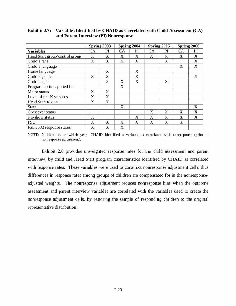
Exhibit 2.7: Variables Identified by CHAID as Correlated with Child Assessment (CA) and Parent Interview (PI) Nonresponse
Spring 2003 Spring 2004 Spring 2005 Spring 2006 Variables CA PI CA PI CA PI CA PI Head Start group/control group X X X X X X X X Child’s race X X X X X X Child’s language X X Home language X X Child’s gender X X X X Child’s age X X X X Program option applied for X Metro status X X Level of pre-K services X X Head Start region X X State X X Crossover status X X X X No-show status X X X X X X PSU X X X X X X X Fall 2002 response status X X X
NOTE: X identifies in which years CHAID identified a variable as correlated with nonresponse (prior to nonresponse adjustment).
Exhibit 2.8 provides unweighted response rates for the child assessment and parent
interview, by child and Head Start program characteristics identified by CHAID as correlated
with response rates. These variables were used to construct nonresponse adjustment cells, thus
differences in response rates among groups of children are compensated for in the nonresponse-
adjusted weights. The nonresponse adjustment reduces nonresponse bias when the outcome
assessment and parent interview variables are correlated with the variables used to create the
nonresponse adjustment cells, by restoring the sample of responding children to the original
representative distribution.
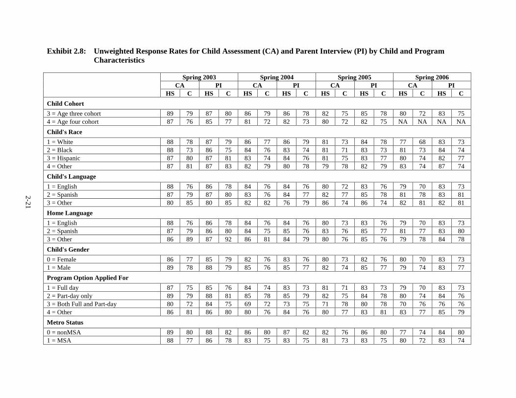
2-21
Exhibit 2.8: Unweighted Response Rates for Child Assessment (CA) and Parent Interview (PI) by Child and Program Characteristics
Spring 2003 Spring 2004 Spring 2005 Spring 2006 CA PI CA PI CA PI CA PI HS C HS C HS C HS C HS C HS C HS C HS C Child Cohort 3 = Age three cohort 89 79 87 80 86 79 86 78 82 75 85 78 80 72 83 75 4 = Age four cohort 87 76 85 77 81 72 82 73 80 72 82 75 NA NA NA NA Child's Race 1 = White 88 78 87 79 86 77 86 79 81 73 84 78 77 68 83 73 2 = Black 88 73 86 75 84 76 83 74 81 71 83 73 81 73 84 74 3 = Hispanic 87 80 87 81 83 74 84 76 81 75 83 77 80 74 82 77 4 = Other 87 81 87 83 82 79 80 78 79 78 82 79 83 74 87 74 Child's Language 1 = English 88 76 86 78 84 76 84 76 80 72 83 76 79 70 83 73 2 = Spanish 87 79 87 80 83 76 84 77 82 77 85 78 81 78 83 81 3 = Other 80 85 80 85 82 82 76 79 86 74 86 74 82 81 82 81 Home Language 1 = English 88 76 86 78 84 76 84 76 80 73 83 76 79 70 83 73 2 = Spanish 87 79 86 80 84 75 85 76 83 76 85 77 81 77 83 80 3 = Other 86 89 87 92 86 81 84 79 80 76 85 76 79 78 84 78 Child's Gender 0 = Female 86 77 85 79 82 76 83 76 80 73 82 76 80 70 83 73 1 = Male 89 78 88 79 85 76 85 77 82 74 85 77 79 74 83 77 Program Option Applied For 1 = Full day 87 75 85 76 84 74 83 73 81 71 83 73 79 70 83 73 2 = Part-day only 89 79 88 81 85 78 85 79 82 75 84 78 80 74 84 76 3 = Both Full and Part-day 80 72 84 75 69 72 73 75 71 78 80 78 70 76 76 76 4 = Other 86 81 86 80 80 76 84 76 80 77 83 81 83 77 85 79 Metro Status 0 = nonMSA 89 80 88 82 86 80 87 82 82 76 86 80 77 74 84 80 1 = MSA 88 77 86 78 83 75 83 75 81 73 83 75 80 72 83 74
2-22
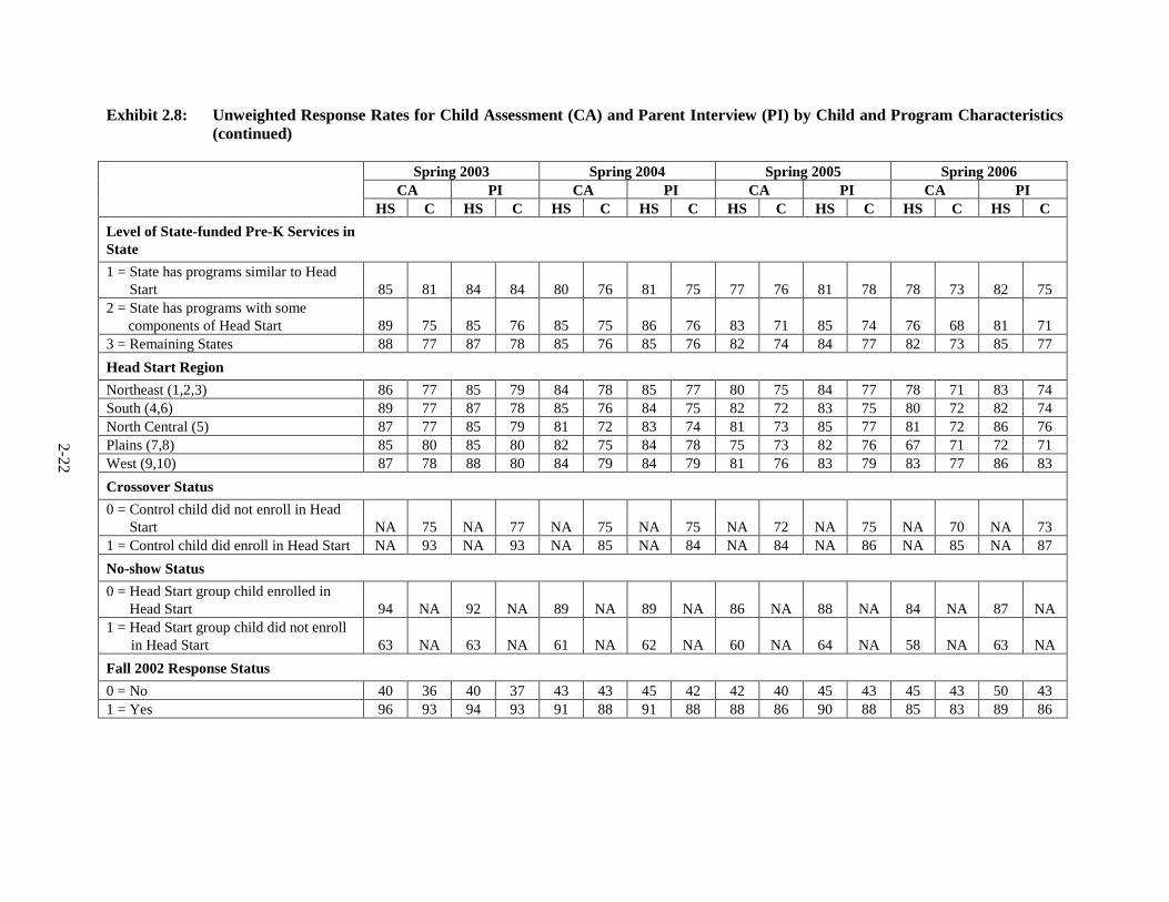
Exhibit 2.8: Unweighted Response Rates for Child Assessment (CA) and Parent Interview (PI) by Child and Program Characteristics (continued)
Spring 2003 Spring 2004 Spring 2005 Spring 2006 CA PI CA PI CA PI CA PI HS C HS C HS C HS C HS C HS C HS C HS C Level of State-funded Pre-K Services in State
1 = State has programs similar to Head Start 85 81 84 84 80 76 81 75 77 76 81 78 78 73 82 75
2 = State has programs with some components of Head Start 89 75 85 76 85 75 86 76 83 71 85 74 76 68 81 71
3 = Remaining States 88 77 87 78 85 76 85 76 82 74 84 77 82 73 85 77 Head Start Region Northeast (1,2,3) 86 77 85 79 84 78 85 77 80 75 84 77 78 71 83 74 South (4,6) 89 77 87 78 85 76 84 75 82 72 83 75 80 72 82 74 North Central (5) 87 77 85 79 81 72 83 74 81 73 85 77 81 72 86 76 Plains (7,8) 85 80 85 80 82 75 84 78 75 73 82 76 67 71 72 71 West (9,10) 87 78 88 80 84 79 84 79 81 76 83 79 83 77 86 83 Crossover Status 0 = Control child did not enroll in Head
Start NA 75 NA 77 NA 75 NA 75 NA 72 NA 75 NA 70 NA 73 1 = Control child did enroll in Head Start NA 93 NA 93 NA 85 NA 84 NA 84 NA 86 NA 85 NA 87 No-show Status 0 = Head Start group child enrolled in
Head Start 94 NA 92 NA 89 NA 89 NA 86 NA 88 NA 84 NA 87 NA 1 = Head Start group child did not enroll
in Head Start 63 NA 63 NA 61 NA 62 NA 60 NA 64 NA 58 NA 63 NA Fall 2002 Response Status 0 = No 40 36 40 37 43 43 45 42 42 40 45 43 45 43 50 43 1 = Yes 96 93 94 93 91 88 91 88 88 86 90 88 85 83 89 86
2-23
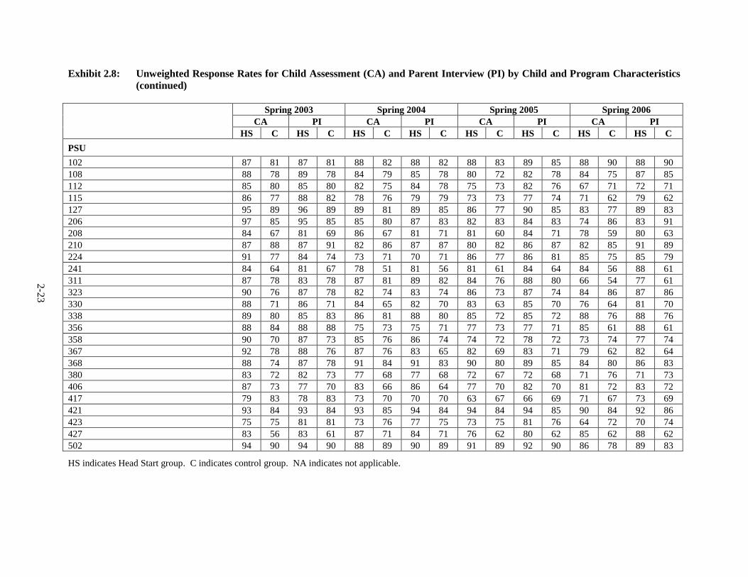
Exhibit 2.8: Unweighted Response Rates for Child Assessment (CA) and Parent Interview (PI) by Child and Program Characteristics (continued)
Spring 2003 Spring 2004 Spring 2005 Spring 2006 CA PI CA PI CA PI CA PI HS C HS C HS C HS C HS C HS C HS C HS C PSU 102 87 81 87 81 88 82 88 82 88 83 89 85 88 90 88 90 108 88 78 89 78 84 79 85 78 80 72 82 78 84 75 87 85 112 85 80 85 80 82 75 84 78 75 73 82 76 67 71 72 71 115 86 77 88 82 78 76 79 79 73 73 77 74 71 62 79 62 127 95 89 96 89 89 81 89 85 86 77 90 85 83 77 89 83 206 97 85 95 85 85 80 87 83 82 83 84 83 74 86 83 91 208 84 67 81 69 86 67 81 71 81 60 84 71 78 59 80 63 210 87 88 87 91 82 86 87 87 80 82 86 87 82 85 91 89 224 91 77 84 74 73 71 70 71 86 77 86 81 85 75 85 79 241 84 64 81 67 78 51 81 56 81 61 84 64 84 56 88 61 311 87 78 83 78 87 81 89 82 84 76 88 80 66 54 77 61 323 90 76 87 78 82 74 83 74 86 73 87 74 84 86 87 86 330 88 71 86 71 84 65 82 70 83 63 85 70 76 64 81 70 338 89 80 85 83 86 81 88 80 85 72 85 72 88 76 88 76 356 88 84 88 88 75 73 75 71 77 73 77 71 85 61 88 61 358 90 70 87 73 85 76 86 74 74 72 78 72 73 74 77 74 367 92 78 88 76 87 76 83 65 82 69 83 71 79 62 82 64 368 88 74 87 78 91 84 91 83 90 80 89 85 84 80 86 83 380 83 72 82 73 77 68 77 68 72 67 72 68 71 76 71 73 406 87 73 77 70 83 66 86 64 77 70 82 70 81 72 83 72 417 79 83 78 83 73 70 70 70 63 67 66 69 71 67 73 69 421 93 84 93 84 93 85 94 84 94 84 94 85 90 84 92 86 423 75 75 81 81 73 76 77 75 73 75 81 76 64 72 70 74 427 83 56 83 61 87 71 84 71 76 62 80 62 85 62 88 62 502 94 90 94 90 88 89 90 89 91 89 92 90 86 78 89 83
HS indicates Head Start group. C indicates control group. NA indicates not applicable.
2-24
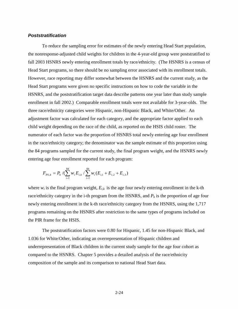
Poststratification
To reduce the sampling error for estimates of the newly entering Head Start population,
the nonresponse-adjusted child weights for children in the 4-year-old group were poststratified to
fall 2003 HSNRS newly entering enrollment totals by race/ethnicity. (The HSNRS is a census of
Head Start programs, so there should be no sampling error associated with its enrollment totals.
However, race reporting may differ somewhat between the HSNRS and the current study, as the
Head Start programs were given no specific instructions on how to code the variable in the
HSNRS, and the poststratification target data describe patterns one year later than study sample
enrollment in fall 2002.) Comparable enrollment totals were not available for 3-year-olds. The
three race/ethnicity categories were Hispanic, non-Hispanic Black, and White/Other. An
adjustment factor was calculated for each category, and the appropriate factor applied to each
child weight depending on the race of the child, as reported on the HSIS child roster. The
numerator of each factor was the proportion of HSNRS total newly entering age four enrollment
in the race/ethnicity category; the denominator was the sample estimate of this proportion using
the 84 programs sampled for the current study, the final program weight, and the HSNRS newly
entering age four enrollment reported for each program:
)(//(84
13,2,1,
84
1,, ∑∑
==
++=i
iiiii
kiikkPS EEEwEwPF
where wi is the final program weight, Ei,k is the age four newly entering enrollment in the k-th
race/ethnicity category in the i-th program from the HSNRS, and Pk is the proportion of age four
newly entering enrollment in the k-th race/ethnicity category from the HSNRS, using the 1,717
programs remaining on the HSNRS after restriction to the same types of programs included on
the PIR frame for the HSIS.
The poststratification factors were 0.80 for Hispanic, 1.45 for non-Hispanic Black, and
1.036 for White/Other, indicating an overrepresentation of Hispanic children and
underrepresentation of Black children in the current study sample for the age four cohort as
compared to the HSNRS. Chapter 5 provides a detailed analysis of the race/ethnicity
composition of the sample and its comparison to national Head Start data.

2-25
Trimming
A final trimming adjustment was made for inordinately large child weights. Very large
weights can substantially increase sampling error, so weights were trimmed back to four times
the average weight to avoid large sampling errors, even though this introduces a small amount of
bias into the survey estimates. However, the amount of trimming was very slight: two percent
or fewer of the child assessment and parent interview weights were trimmed back each year. An
analysis of the trimmed cases showed that most extremely large weights were due primarily to
some large centers being undersampled, that is, only a few children were sampled, perhaps due
to near-saturation. The final child weight can be written as:
Final Child Weight = (Overall Child Base Wt) x (Child Nonresponse Adjustment Factor) x (Poststratification Factor) x (Trimming Factor)
where the overall child base weight reflects the probability of selecting the PSU, program,
center, and child within center. When the final child weight is applied, the Head Start and
control groups, each separately represent the entire newly entering Head Start population in fall
2002. Sample estimates of the size of the newly entering Head Start population that year are
given in Exhibit 2.9 in the “Sum of Final Weights” column; Exhibit 2.10 contains unweighted
and weighted response rates at each data collection period from fall 2002 through spring 2006
for the child assessment and the parent interview. These response rates are conditional on the
sampled centers and programs where random assignment of Head Start applicants was permitted;
they do not represent coverage rates of the Head Start newly entering population.
2-26
Exhibit 2.9: Final Sampling Weights, Fall 2002 through Spring 2006
Time Period Number of
Respondents Sum of Final
Weights 95% Confidence
Interval
Coefficient of Variation
(CV) of Final Weights (%)
Fall 2002 Child Assessment
Head Start Group 2,360 422,686 (356,049, 489,323) 86 Control Group 1,363 413,258 (351,102, 475,415) 77
Parent Interview Head Start Group 2,489 423,086 (357,343, 488,829) 85 Control Group 1,526 414,214 (350,637, 477,792) 78
Spring 2003 Child Assessment
Head Start Group 2,441 426,834 (355,935, 497,733) 86 Control Group 1,457 418,907 (357,034, 480,781) 88
Parent Interview Head Start Group 2,404 427,536 (358,052, 497,020) 86 Control Group 1,483 419,772 (357,437, 482,107) 88
Spring 2004 Child Assessment
Head Start Group 2,331 426,911 (361,442, 492,380) 88 Control Group 1,431 421,590 (355,310, 487,869) 91
Parent Interview Head Start Group 2,342 427,732 (363,504, 491,959) 88 Control Group 1,433 423,218 (359,210, 487,225) 91
Spring 2005 Child Assessment
Head Start Group 2,254 428,291 (363,741, 492,842) 83 Control Group 1,385 418,834 (353,454, 484,215) 83
Parent Interview Head Start Group 2,327 428,137 (362,525, 493,750) 83 Control Group 1,438 419,759 (355,596, 483,921) 84
Spring 2006 (age 3 cohort only) Child Assessment
Head Start Group 1,218 225,766 (189,555, 261,977) 84 Control Group 742 224,475 (183,758, 265,191) 84
Parent Interview Head Start Group 1,274 225,766 (188,671, 262,861) 85 Control Group 772 224,475 (186,606, 262,344) 82

2-27
Exhibit 2.10: Unweighted and Weighted Cross-Sectional Response Rates by Wave
Unweighted Cross-Sectional Response Rates (%) by Wave
Fall 2002 2003 2004 2005 2006 Instrument Age 3 Age 4 Age 3 Age 4 Age 3 Age 4 Age 3 Age 4 Age 3 Age 4
Child Assessment Head Start Group 87 85 89 87 86 81 82 80 80 NA Control Group 74 74 79 76 79 72 75 72 72 NA
Parent Interview Head Start Group 92 89 87 85 86 82 85 82 83 NA Control Group 84 82 80 77 78 73 78 75 75 NA
Weighted Cross-Sectional Response Rates (%) by Wave
Fall 2002 2003 2004 2005 2006 Instrument Age 3 Age 4 Age 3 Age 4 Age 3 Age 4 Age 3 Age 4 Age 3 Age 4
Child Assessment Head Start Group 87 86 89 87 87 81 82 79 81 NA Control Group 76 77 80 77 79 74 77 73 74 NA
Parent Interview Head Start Group 93 90 88 85 86 82 85 82 85 NA Control Group 84 84 81 79 79 75 79 75 76 NA
NA indicates not applicable.
Teacher Survey/Teacher Child Rating Weights
Children who were attending a pre-K program (either Head Start or some other type of
program), kindergarten, or first grade were eligible for the Teacher Survey and Teacher’s/Care
Provider’s Child Report (see Chapter 2 in the Final Report for a description of these forms).
Children who were receiving only their parent’s care at home were not eligible for these surveys.
A cross-sectional weight was created each spring for children with a completed Teacher Survey
and Teacher Child Report, and a completed child assessment and parent interview as well. The
child’s base weight was first adjusted for nonresponse to both the child assessment and parent
interview, then poststratified and trimmed as described above for the child assessment and parent
interview weights. This weight was then adjusted for nonresponse to both the teacher survey and
teacher child rating, using CHAID as described above to identify variables correlated with
nonresponse.
2-28
Classroom Observation Weights
In spring 2003 and 2004, only pre-K children attending a Head Start or other type of pre-
K center (including another home) were eligible for classroom observations (see Chapter 2 in the
Final Report for a description of this data type). Thus in spring 2004, members of the age four
cohort who were in kindergarten do not have classroom observations. No classroom
observations were conducted in spring 2005 or 2006 since most children were in kindergarten or
first grade by then. A cross-sectional classroom observation weight was calculated for every
child with a completed classroom observation, child assessment, and parent interview that year,
in spring 2003 and 2004. This was done by adjusting the child’s base weight first for
nonresponse to the child assessment and parent interview each spring, poststratifying and
trimming as before, then adjusting for “nonresponse” to the classroom observations, using
CHAID to identify variables correlated with nonresponse.
Director Interview Weights
The director interview was conducted at Head Start centers or other types of pre-K
centers in spring 2003 and 2004 where the sampled children attended (see Chapter 2 in the Final
Report for a description of this instrument). No director interviews were conducted in spring
2005 and 2006 as most children were attending school by then. A cross-sectional director
interview weight was calculated for every child with a completed classroom observation, child
assessment, and parent interview that year, in spring 2003 and 2004. This was done by adjusting
the child’s base weight first for nonresponse to the child assessment and parent interview each
spring, poststratifying and trimming as before, then adjusting for “nonresponse” to the director
interview, using CHAID to identify variables correlated with nonresponse.
Response Rates and Variables Correlated with Teacher, Classroom, and Director Interview Response Rates
The response rates for the teacher survey/teacher child report, classroom observations,
and director interview are provided in Exhibit 2.11. The response rates are based on only the
children eligible for each instrument among those with a complete child assessment and parent
interview that year. The variables identified by CHAID as correlated with having a completed
teacher survey and teacher child report, classroom observations, or a completed director
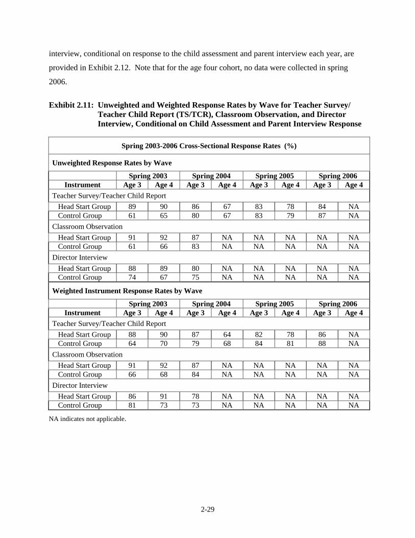
2-29
interview, conditional on response to the child assessment and parent interview each year, are
provided in Exhibit 2.12. Note that for the age four cohort, no data were collected in spring
2006.
Exhibit 2.11: Unweighted and Weighted Response Rates by Wave for Teacher Survey/
Teacher Child Report (TS/TCR), Classroom Observation, and Director Interview, Conditional on Child Assessment and Parent Interview Response
Spring 2003-2006 Cross-Sectional Response Rates (%)
Unweighted Response Rates by Wave
Spring 2003 Spring 2004 Spring 2005 Spring 2006 Instrument Age 3 Age 4 Age 3 Age 4 Age 3 Age 4 Age 3 Age 4
Teacher Survey/Teacher Child Report Head Start Group 89 90 86 67 83 78 84 NA Control Group 61 65 80 67 83 79 87 NA
Classroom Observation Head Start Group 91 92 87 NA NA NA NA NA Control Group 61 66 83 NA NA NA NA NA
Director Interview Head Start Group 88 89 80 NA NA NA NA NA Control Group 74 67 75 NA NA NA NA NA
Weighted Instrument Response Rates by Wave
Spring 2003 Spring 2004 Spring 2005 Spring 2006 Instrument Age 3 Age 4 Age 3 Age 4 Age 3 Age 4 Age 3 Age 4
Teacher Survey/Teacher Child Report Head Start Group 88 90 87 64 82 78 86 NA Control Group 64 70 79 68 84 81 88 NA
Classroom Observation Head Start Group 91 92 87 NA NA NA NA NA Control Group 66 68 84 NA NA NA NA NA
Director Interview Head Start Group 86 91 78 NA NA NA NA NA Control Group 81 73 73 NA NA NA NA NA
NA indicates not applicable.
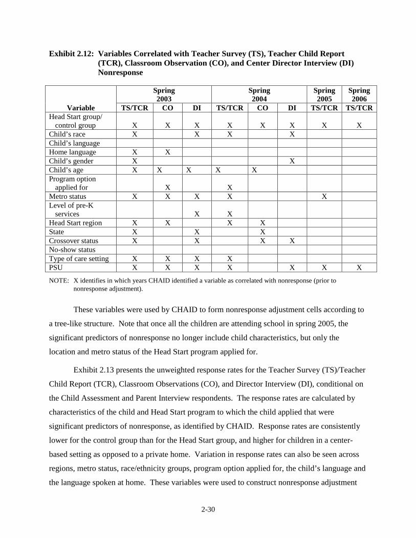
2-30
Exhibit 2.12: Variables Correlated with Teacher Survey (TS), Teacher Child Report (TCR), Classroom Observation (CO), and Center Director Interview (DI) Nonresponse
Spring
2003 Spring 2004
Spring 2005
Spring 2006
Variable TS/TCR CO DI TS/TCR CO DI TS/TCR TS/TCR Head Start group/
control group X X X X X X X X Child’s race X X X X Child’s language Home language X X Child’s gender X X Child’s age X X X X X Program option
applied for X X Metro status X X X X X Level of pre-K
services X X Head Start region X X X X State X X X Crossover status X X X X No-show status Type of care setting X X X X PSU X X X X X X X
NOTE: X identifies in which years CHAID identified a variable as correlated with nonresponse (prior to nonresponse adjustment).
These variables were used by CHAID to form nonresponse adjustment cells according to
a tree-like structure. Note that once all the children are attending school in spring 2005, the
significant predictors of nonresponse no longer include child characteristics, but only the
location and metro status of the Head Start program applied for.
Exhibit 2.13 presents the unweighted response rates for the Teacher Survey (TS)/Teacher
Child Report (TCR), Classroom Observations (CO), and Director Interview (DI), conditional on
the Child Assessment and Parent Interview respondents. The response rates are calculated by
characteristics of the child and Head Start program to which the child applied that were
significant predictors of nonresponse, as identified by CHAID. Response rates are consistently
lower for the control group than for the Head Start group, and higher for children in a center-
based setting as opposed to a private home. Variation in response rates can also be seen across
regions, metro status, race/ethnicity groups, program option applied for, the child’s language and
the language spoken at home. These variables were used to construct nonresponse adjustment
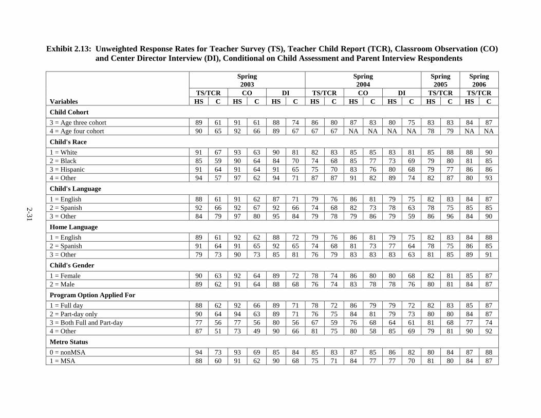
2-31
Exhibit 2.13: Unweighted Response Rates for Teacher Survey (TS), Teacher Child Report (TCR), Classroom Observation (CO) and Center Director Interview (DI), Conditional on Child Assessment and Parent Interview Respondents
Spring
2003 Spring 2004
Spring 2005
Spring 2006
TS/TCR CO DI TS/TCR CO DI TS/TCR TS/TCR Variables HS C HS C HS C HS C HS C HS C HS C HS C Child Cohort 3 = Age three cohort 89 61 91 61 88 74 86 80 87 83 80 75 83 83 84 87 4 = Age four cohort 90 65 92 66 89 67 67 67 NA NA NA NA 78 79 NA NA Child's Race 1 = White 91 67 93 63 90 81 82 83 85 85 83 81 85 88 88 90 2 = Black 85 59 90 64 84 70 74 68 85 77 73 69 79 80 81 85 3 = Hispanic 91 64 91 64 91 65 75 70 83 76 80 68 79 77 86 86 4 = Other 94 57 97 62 94 71 87 87 91 82 89 74 82 87 80 93 Child's Language 1 = English 88 61 91 62 87 71 79 76 86 81 79 75 82 83 84 87 2 = Spanish 92 66 92 67 92 66 74 68 82 73 78 63 78 75 85 85 3 = Other 84 79 97 80 95 84 79 78 79 86 79 59 86 96 84 90 Home Language
1 = English 89 61 92 62 88 72 79 76 86 81 79 75 82 83 84 88 2 = Spanish 91 64 91 65 92 65 74 68 81 73 77 64 78 75 86 85 3 = Other 79 73 90 73 85 81 76 79 83 83 83 63 81 85 89 91 Child's Gender 1 = Female 90 63 92 64 89 72 78 74 86 80 80 68 82 81 85 87 2 = Male 89 62 91 64 88 68 76 74 83 78 78 76 80 81 84 87 Program Option Applied For 1 = Full day 88 62 92 66 89 71 78 72 86 79 79 72 82 83 85 87 2 = Part-day only 90 64 94 63 89 71 76 75 84 81 79 73 80 80 84 87 3 = Both Full and Part-day 77 56 77 56 80 56 67 59 76 68 64 61 81 68 77 74 4 = Other 87 51 73 49 90 66 81 75 80 58 85 69 79 81 90 92 Metro Status 0 = nonMSA 94 73 93 69 85 84 85 83 87 85 86 82 80 84 87 88 1 = MSA 88 60 91 62 90 68 75 71 84 77 77 70 81 80 84 87
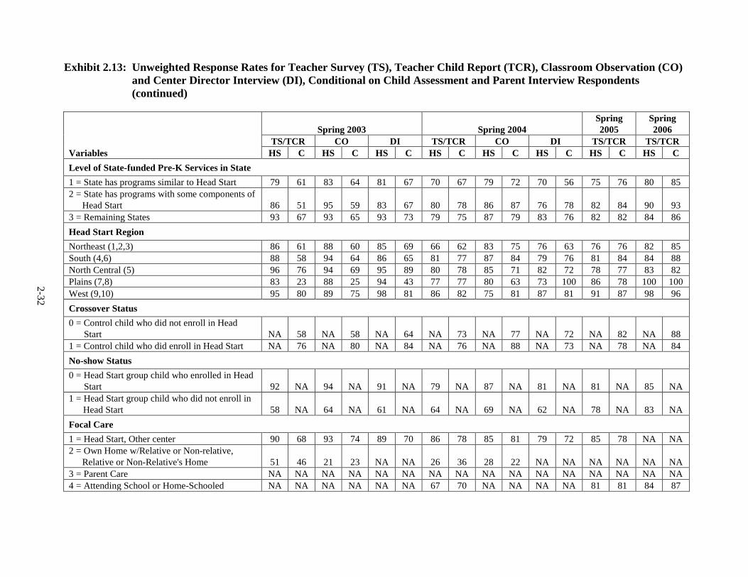
2-32
Exhibit 2.13: Unweighted Response Rates for Teacher Survey (TS), Teacher Child Report (TCR), Classroom Observation (CO) and Center Director Interview (DI), Conditional on Child Assessment and Parent Interview Respondents (continued)
Spring 2003 Spring 2004 Spring 2005
Spring 2006
TS/TCR CO DI TS/TCR CO DI TS/TCR TS/TCR Variables HS C HS C HS C HS C HS C HS C HS C HS C Level of State-funded Pre-K Services in State 1 = State has programs similar to Head Start 79 61 83 64 81 67 70 67 79 72 70 56 75 76 80 85 2 = State has programs with some components of
Head Start 86 51 95 59 83 67 80 78 86 87 76 78 82 84 90 93 3 = Remaining States 93 67 93 65 93 73 79 75 87 79 83 76 82 82 84 86 Head Start Region Northeast (1,2,3) 86 61 88 60 85 69 66 62 83 75 76 63 76 76 82 85 South (4,6) 88 58 94 64 86 65 81 77 87 84 79 76 81 84 84 88 North Central (5) 96 76 94 69 95 89 80 78 85 71 82 72 78 77 83 82 Plains (7,8) 83 23 88 25 94 43 77 77 80 63 73 100 86 78 100 100 West (9,10) 95 80 89 75 98 81 86 82 75 81 87 81 91 87 98 96 Crossover Status 0 = Control child who did not enroll in Head
Start NA 58 NA 58 NA 64 NA 73 NA 77 NA 72 NA 82 NA 88 1 = Control child who did enroll in Head Start NA 76 NA 80 NA 84 NA 76 NA 88 NA 73 NA 78 NA 84 No-show Status 0 = Head Start group child who enrolled in Head
Start 92 NA 94 NA 91 NA 79 NA 87 NA 81 NA 81 NA 85 NA 1 = Head Start group child who did not enroll in
Head Start 58 NA 64 NA 61 NA 64 NA 69 NA 62 NA 78 NA 83 NA Focal Care 1 = Head Start, Other center 90 68 93 74 89 70 86 78 85 81 79 72 85 78 NA NA 2 = Own Home w/Relative or Non-relative,
Relative or Non-Relative's Home 51 46 21 23 NA NA 26 36 28 22 NA NA NA NA NA NA 3 = Parent Care NA NA NA NA NA NA NA NA NA NA NA NA NA NA NA NA 4 = Attending School or Home-Schooled NA NA NA NA NA NA 67 70 NA NA NA NA 81 81 84 87
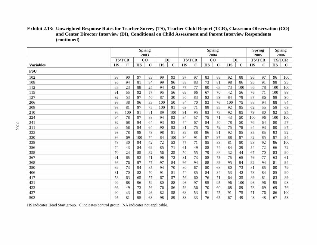
2-33
Exhibit 2.13: Unweighted Response Rates for Teacher Survey (TS), Teacher Child Report (TCR), Classroom Observation (CO) and Center Director Interview (DI), Conditional on Child Assessment and Parent Interview Respondents (continued)
Spring
2003 Spring 2004
Spring 2005
Spring 2006
TS/TCR CO DI TS/TCR CO DI TS/TCR TS/TCR Variables HS C HS C HS C HS C HS C HS C HS C HS C PSU 102 98 90 97 83 99 93 97 97 83 88 92 88 96 97 96 100 108 95 94 81 84 99 96 88 83 73 81 98 86 95 91 98 95 112 83 23 88 25 94 43 77 77 80 63 73 100 86 78 100 100 115 91 55 92 57 95 56 69 66 67 70 42 56 76 71 100 88 127 92 53 97 46 87 30 86 83 92 89 84 79 87 86 98 96 206 98 38 96 33 100 50 84 70 93 76 100 75 88 94 88 84 208 98 81 97 75 100 91 63 71 89 85 92 85 62 55 58 63 210 98 100 91 81 89 100 91 95 83 73 92 85 79 80 92 95 224 94 78 97 88 94 93 84 57 75 71 43 50 100 96 100 100 241 92 68 94 64 93 93 74 67 84 50 78 50 76 64 80 57 311 83 58 94 64 90 83 81 75 75 79 75 78 84 93 80 87 323 98 78 98 78 98 81 89 88 96 91 92 85 85 85 93 92 330 98 69 100 74 84 100 94 91 97 97 88 97 82 85 97 94 338 78 30 94 42 72 53 77 71 85 83 81 80 93 92 96 100 356 74 43 84 69 85 71 61 49 88 74 84 39 54 72 66 72 358 70 24 85 32 56 25 50 55 79 88 32 44 67 70 83 90 367 91 65 93 71 96 72 81 73 88 75 75 65 76 77 63 61 368 98 76 97 77 97 84 96 94 88 89 95 94 92 94 81 94 380 89 73 94 85 94 70 80 67 80 68 80 73 81 85 80 79 406 81 70 82 70 91 81 74 85 84 84 53 42 78 84 85 90 417 53 63 65 57 67 57 56 60 76 71 64 35 89 81 83 89 421 99 68 96 59 80 88 96 97 95 95 96 100 96 96 95 98 423 66 49 73 56 76 56 59 56 70 60 68 59 78 69 69 76 427 90 43 92 46 82 58 63 53 91 75 91 75 71 76 86 100 502 95 81 95 68 98 89 33 33 76 65 67 49 48 48 67 58
HS indicates Head Start group. C indicates control group. NA indicates not applicable.
2-34
cells for the calculation of nonresponse adjustment factors, thus differences in response rates
among groups of children are compensated for in the nonresponse-adjusted weights. The
nonresponse adjustment reduces nonresponse bias when the outcomes are correlated with the
variables used to create the nonresponse adjustment cells, by restoring the sample of responding
children to the original representative distribution.
Longitudinal Weights
Two longitudinal weights were also calculated for each child for use in growth curve
analysis with multi-level models (see Chapter 5). Children with two or more completed
assessments in the time period from fall 2002 through spring 2006 were given a weight so they
could represent the population of newly entering Head Start applicants in growth curve analysis
requiring at least two time points per child. Two time points are the minimum for representing
linear growth. Most students will have greater than two time points. Another weight was
calculated for children who completed three or more assessments in the same time period for use
in growth curve analysis requiring at least three time points per child. Three time points are the
minimum for representing quadratic growth. Most students will have more than three time
points so average growth can be adequately estimated. The variables identified by CHAID as
correlated with response for the longitudinal weights were the Head Start indicator, no-show
status (children assigned to Head Start but did not participate), crossover status (children
assigned to the control group but who participated in Head Start anyway), program option
applied for, level of pre-K programs in the state, urban status, Head Start region, and PSU. Of
the original sample of 4,667 children, 87 percent completed two or more assessments, and 81
percent completed three or more assessments. Each longitudinal weight was created by adjusting
the child’s overall base weight for longitudinal nonresponse, poststratifiying the nonresponse-
adjusted weight to the HSNRS (for the age four cohort), and trimming the poststratified weight
for 1.5 percent of the respondents whose weight exceeded four times the average weight.
Exhibit 2.14 contains unweighted longitudinal response rates for children with two or
more child assessments in the fall 2002-spring 2006 period, and for children with three or more
assessments. It can be seen that attrition rates are higher for the control group and there is
considerable variation across locations in attrition rates.
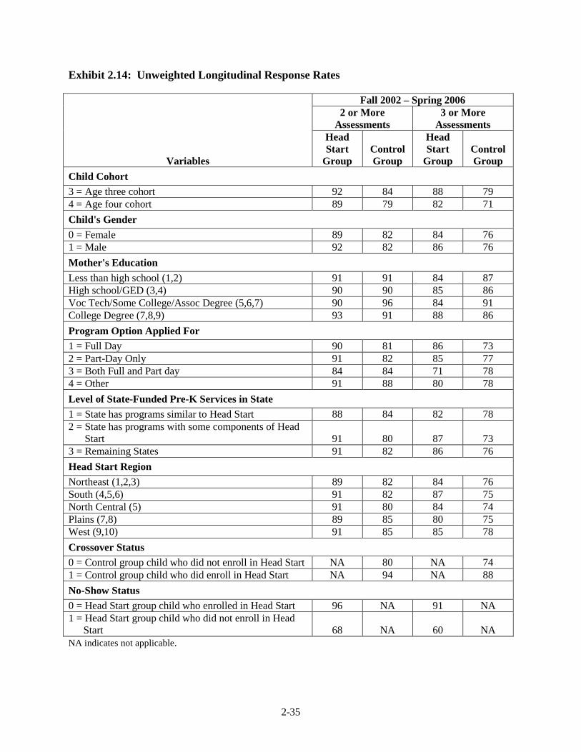
2-35
Exhibit 2.14: Unweighted Longitudinal Response Rates Fall 2002 – Spring 2006 2 or More
Assessments 3 or More
Assessments
Variables
Head Start
Group Control Group
Head Start
Group Control Group
Child Cohort 3 = Age three cohort 92 84 88 79 4 = Age four cohort 89 79 82 71 Child's Gender 0 = Female 89 82 84 76 1 = Male 92 82 86 76 Mother's Education Less than high school (1,2) 91 91 84 87 High school/GED (3,4) 90 90 85 86 Voc Tech/Some College/Assoc Degree (5,6,7) 90 96 84 91 College Degree (7,8,9) 93 91 88 86 Program Option Applied For 1 = Full Day 90 81 86 73 2 = Part-Day Only 91 82 85 77 3 = Both Full and Part day 84 84 71 78 4 = Other 91 88 80 78 Level of State-Funded Pre-K Services in State 1 = State has programs similar to Head Start 88 84 82 78 2 = State has programs with some components of Head
Start 91 80 87 73 3 = Remaining States 91 82 86 76 Head Start Region Northeast (1,2,3) 89 82 84 76 South (4,5,6) 91 82 87 75 North Central (5) 91 80 84 74 Plains (7,8) 89 85 80 75 West (9,10) 91 85 85 78 Crossover Status 0 = Control group child who did not enroll in Head Start NA 80 NA 74 1 = Control group child who did enroll in Head Start NA 94 NA 88 No-Show Status 0 = Head Start group child who enrolled in Head Start 96 NA 91 NA 1 = Head Start group child who did not enroll in Head
Start 68 NA 60 NA NA indicates not applicable.
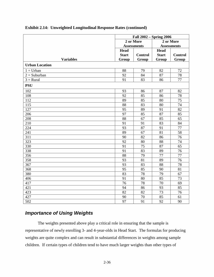
2-36
Exhibit 2.14: Unweighted Longitudinal Response Rates (continued) Fall 2002 – Spring 2006 2 or More
Assessments 2 or More
Assessments
Variables
Head Start
Group Control Group
Head Start
Group Control Group
Urban Location 1 = Urban 88 79 82 72 2 = Suburban 92 84 87 78 3 = Rural 91 83 86 77 PSU 102 93 86 87 82 108 92 85 86 78 112 89 85 80 75 115 88 83 80 74 127 95 89 91 82 206 97 85 87 85 208 88 67 85 65 210 91 91 83 84 224 93 87 91 77 241 89 67 81 58 311 90 82 86 76 323 92 80 88 74 330 91 75 87 65 338 91 83 89 76 356 88 79 77 77 358 93 81 89 76 367 93 83 88 78 368 95 85 90 81 380 83 78 79 67 406 91 80 85 73 417 76 78 70 69 421 94 86 93 85 423 82 82 73 76 427 90 70 85 61 502 97 91 92 90
Importance of Using Weights
The weights presented above play a critical role in ensuring that the sample is
representative of newly enrolling 3- and 4-year-olds in Head Start. The formulas for producing
weights are quite complex and can result in substantial differences in weights among sample
children. If certain types of children tend to have much larger weights than other types of
2-37
children, and if the weights are not used in the analysis, then the types of children with large
weights will be underrepresented in the analysis relative to the population of all newly entering
Head Start children. This can lead to serious bias in impact estimates. Thus, we strongly
recommend that weights be used in all analyses.
Calculating Correct Standard Errors
Estimates obtained from the Head Start Impact Study will differ from the true population
parameters because they are based on a randomly chosen subset of the population, rather than on
a complete census of all newly entering Head Start children. This type of error is known as
sampling error or variance. The differences between the estimates and the true population values
can also be caused by nonsampling error. Nonsampling errors can result from many causes, such
as measurement error, nonresponse, sampling frame errors, respondent error, and differences
among interviewers. In general, the magnitude of nonsampling error is difficult to assess from
the sample. The precision of an estimate is measured by the standard error (defined as the square
root of the variance due to sampling). The calculation of the standard error must reflect not only
the sample size on which the estimate is based, but the manner in which the sample was drawn.
Otherwise, the standard errors can be misleading and result in incorrect confidence intervals and
p-values in hypothesis testing. The study’s sampling involved stratification, clustering, and
unequal probabilities of selection, all of which must be reflected in the standard error
calculations.
Two commonly used variance estimation methods for complex surveys involving multi-
stage sampling are replication and linearization (Wolter, 1985). Replication methods work by
dividing the sample into subsample replicates that mirror the design of the sample. A weight is
calculated for each replicate using the same procedures as for the full-sample weight. This
produces a set of replicate weights for each sampled child. To calculate the standard error of a
survey estimate, the estimate is first calculated for each replicate using the replicate weight and
the same form of estimator as for the full sample. The variation among the replicates is then
used to estimate the variance for the full sample estimate. In the linearization approach, a
nonlinear estimator is approximated by a linear function and a formula derived for the variance
of the linear approximation. Replication has the advantage that it can reflect the different
features of the weighting and estimation by simply repeating all steps separately for each

2-38
replicate. For linearization, a specific formula is needed for each estimator, and the formula will
differ depending on the type of estimator and sample design. On the other hand, finite
population correction factors are often easier to account for using linearization estimators.
However, for linear estimators, or nonlinear estimators that are formed by combinations of linear
functions, replication variance estimators are often little different numerically from linearization
variance estimators.
For the current study, a set of 76 jackknife replicate weights was created for each child
for use in the calculation of all standard errors. Normally, stratified jackknife replicate weights
are created by dropping out one PSU at a time, setting the replicate weights for sampled units in
the dropped PSU to zero, multiplying the full-sample weights of sampled units in the remaining
PSUs in the stratum by a factor of nh / (nh-1), where nh is the number of PSUs in the h-th stratum,
and leaving the full-sample weights for sampled units in the remaining strata unchanged.
However, because only 25 PSUs were sampled at the first stage (one per stratum), only 27
replicate weights could be created (in the one certainty PSU, two additional replicates could be
formed by forming two “pseudo-PSUs” based on program groups). To improve the stability of
the variance estimates, the second-stage sampling units, namely Head Start program groups,
were used as the “drop unit” in creating replicates. This resulted in 76 replicate weights per child
and 51 degrees of freedom for variance estimation (i.e., 76 PSUs – 25 strata). Because the
between-PSU component of variance is ignored in doing this, the resulting variance estimates
will be slight underestimates if the between-PSU variability is small relative to the within-PSU
variability. The validity of this hypothesis was investigated by creating a second set of 27
replicate weights based on the 25 PSUs, which includes the between-PSU component, but has
fewer degrees of freedom. By calculating the average ratio of the variance from the set of
replicate weights based on the 25 PSUs to the variance from the set based on the 76 program
groups, we were able to estimate the relative size of the between-PSU component. The ratio of
variances was calculated for several child assessment means (PPVT, Elision, Woodcock-Johnson
Applied, Oral Comprehension, Spelling, and Letter-Word) by age and gender within the
combined test language groups English and Spanish, then averaged across tests. For fall 2002
scores, the between-PSU component was estimated to be 15 percent of the total variance, and for
spring 2003 scores, this component was estimated to be 28 percent of the total variance. Thus,
the standard error estimates for means produced from the set of 76 replicate weights may be too
2-39
small. However, for estimates of differences between Head Start group and control group
means, the between-PSU component of variance is expected to be very small because of the high
correlation between PSU level estimates, since the Head Start and control groups come from the
same PSUs. Formally stated, CTCTCTPSU yy σρσσσσ 2)( 222 −+=− so that as ρ approaches one,
the between-PSU component of the total variance, 2PSUσ , approaches zero. Therefore, the
standard error estimates for differences between Head Start group and control group means using
the 76 replicate weights can be expected to differ from the total variance by less than 15 percent.
For spring 2003, the between-PSU component of variance for differences between Head Start
group and control group means was estimated to be less than seven percent of the total variance
for seven child assessment outcomes.
Estimation for Puerto Rico as a separate analysis domain is problematic due to small
sample sizes. As it turns out, there were three Head Start programs sampled in Puerto Rico, 22
centers, and 180 to 190 children (roughly equally split between age three and four) with
completed assessments and a parent interview each spring. From this sample, it is generally
possible to produce estimates of unadjusted mean impacts for assessment scores and parent
interview outcomes. These unadjusted impact estimates are simple differences in means
between the Head Start and control groups. However, the sample sizes in Puerto Rico are too
small to permit adjusted estimates from a regression model containing child covariates to be
made. Variance estimation for Puerto Rico as a separate analysis domain is especially
problematic because only three programs were sampled, leaving insufficient degrees of freedom
to estimate standard errors. (The degrees of freedom are based on the number of first-stage
sampling units, not the number of sampled children.) A special set of 22 jackknife replicate
weights was created for children in Puerto Rico to permit variance estimation for child
assessment and parent interview outcomes by treating the 22 centers as the first-stage sampling
units and the three programs as strata. The special replicate weights provide 19 degrees of
freedom for variance estimation (22-3=19). While this is still quite small, calculation of standard
errors becomes at least feasible. However, these standard error estimates omit the between-
program component of variance and may be underestimates of the true standard error. They are
also likely to be quite unstable, especially for the age three cohort, where the number of centers
in Puerto Rico was reduced from 22 to just the 16 that admitted three-year-olds; consequently the

2-40
number of replicates is reduced from 22 to 16, with only 13 degrees of freedom available for
variance estimation. Therefore, caution should be used in interpreting results of hypothesis
testing based on these estimates.
Another issue arising in the calculation of standard errors is the application of the finite
population correction factor (fpc), where the fpc is defined as one minus the sampling fraction.
For multistage designs, the application of the fpc in jackknife replication will cause
underestimation of the variance. On the other hand, ignoring the fpc will lead to a slight
overestimation of the standard errors, which is a generally accepted practice. In the current
study, the average sampling fraction for sampling PSUs was about 0.2, while the average
sampling fraction for sampling program groups within PSUs was about 0.4. However, as
discussed above, standard errors for impact estimates are already slight underestimates due to the
omission of the between-PSU component of variance in setting up the replicate weights;
therefore, it did not seem advisable to incorporate an fpc, which would have increased the
negative bias in the standard error estimates. In any case, the SUDAAN software we used (see
below) does not allow for incorporation of an fpc with replication methods.
Incorporating Weights and Standard Errors in the Impact Analyses
The easiest way for analysts to incorporate the weights and correct standard errors into
their analyses is to use software designed for analysis of complex survey data. Such software
packages include WesVar, SUDAAN, Stata, and the new survey procedures (proc surveymeans,
proc surveyfreq, proc surveyreg, proc surveylogistic) in SAS version 9. Most estimation and
modeling can be done with one of these packages. WesVar uses replication methods (jackknife,
Balanced Repeated Replication (BRR)), and SAS version 9 uses linearization. SUDAAN and
Stata offer both linearization and replication.
All analyses in this report were done using SUDAAN version 9 with jackknife
replication, with the exception of the subgroup regression-adjusted impact estimates for binary
outcomes and multi-level modeling. Due to a bug in the SUDAAN software pertaining to the
calculation of predicted marginals for subgroups, the regression-adjusted subgroup impact
estimates for binary outcomes and their standard errors were calculated using an in-house SAS
program with jackknife replication, following the formula for subgroup-predicted marginals in
Graubard & Korn (1999) (see Chapter 5). Hypothesis testing of differences in the regression-

2-41
adjusted subgroup estimates for binary outcomes also was conducted using the in-house SAS
program. For multi-level modeling with survey weights, we used the software package HLM
version 6 because it uses the Pfeffermann (see Pfeffermann, et al., 1998) method of handling
survey weights. A recently available alternative that we did not use but that also uses the
Pfeffermann method of applying survey weights in multilevel models is GLLAMM, a user-
written Stata procedure (Rabe-Hesketh Skrondal, 2005). Both HLM and GLLAMM use model-
based variance component estimation assuming a super population model.
2-42
References Cochran, W. G. (1977). Sampling techniques. New York: Wiley & Sons. Graubard, B., & Korn, E. (1999). Predictive margins with survey data, Biometrics, 55, 652-659. Oh, H. L. & Scheuren, F. J. (1987). Modified raking ratio estimation. Survey Methodology, 13,
209-219. Pfeffermann, D., Skinner, C., Goldstein, H. & Rasbash, J. (1998). Weighting for unequal
selection probabilities in multilevel models, Journal of the Royal Statistical Society, series B, 60(1), 23-40.
Rabe-Hesketh, S., & Skrondal, A. (2005). Multilevel and longitudinal modeling using stata.
College Station, TX: StataCorp. Raudenbush, S. W., Bryk, A. S., Cheong, Y. K. and Congdon, R. T., Jr. (2004). HLM6:
Hierarchical linear and nonlinear modeling. Lincolnwood, IL: Scientific Software International.
SUDAAN. (2005). SUDAAN user's manual, Release 9.0. Research Triangle Park, NC:
Research Triangle Institute. Stata. (2005). Stata statistical software: Release 9.0. College Station, TX: StataCorp. Wolter, K. (1985). Introduction to variance estimation. New York: Springer-Verlag. WesVar. (2003). WesVarTM 4.2 user’s guide. Rockville, MD: Westat.

3-1
Chapter 3: Outcome Measurement and Psychometrics
Introduction
In this study, child outcomes provide measures of how well Head Start and non-Head
Start preschool programs, or other child care, are achieving the goal of assisting children to be
physically, socially, and educationally ready for success in school. This study used direct child
assessments, as well as parent and teacher assessments of children’s skills and achievement. The
direct child assessment battery in the Head Start Impact Study focused on language and literacy
including vocabulary, reading and writing skills, oral comprehension and phonological
awareness, as well as math skills. The 45-60 minutes child assessment battery was typically
administered one-on-one by specially trained assessors in the child’s main care setting during the
preschool years (i.e., where the child spent the most time Monday through Friday between the
hours of 9 am and 3 pm) and in the child’s home during the kindergarten and 1st grade years.
This chapter provides detailed information regarding the cognitive assessments utilized in
this study, as well as psychometric and ICC (intraclass correlations) information on all domains
measured. The chapter provides information on: (1) discussion of the treatment of non-English
speaking children; (2) description of the various assessments used throughout the period of the
Head Start Impact Study (fall 2002 through spring 2006); (3) discussion of certain test
adaptations that were implemented to reduce the burden of testing on individual children;
(4) review of IRT scoring used for the PPVT, TVIP, and CTOPPP tests; (5) a review of scoring
procedures used for the few non-standardized tests that were included in the test battery;
(6) description of composite outcome measures that used combinations of selected direct
assessment scales; (7) description of socio-emotional, parenting, and health outcomes; and
(8) psychometric and ICC information for the all outcome measures.
Language of Assessment
At the time of the baseline assessments in fall 2002, the assessor asked the main care
provider (i.e., the teacher or other care provider if the child was in child care or the parent if the

3-2
child was not in child care),6
What language does the child speak most often at home (English, Spanish, or other specified language)?
the following questions (i.e., the Language Decision Form) to
determine the appropriate language of assessment:
What language does the child speak most often at this child care setting (English, Spanish, or other specified language)?
What language does it appear this child prefers to speak (English, Spanish, or other specified language)?
If two or more of the three responses to the above questions were English or Spanish, the child
was tested in that language. For children requiring assessment in Spanish, the assessor
administered a bilingual child assessment that included the complete fall 2002 Spanish
assessment battery and two English tests (the Peabody Picture Vocabulary Test (PPVT) and the
Woodcock-Johnson III Tests of Achievement Letter-Word Identification test). In spring 2003
and in subsequent data collection periods, the bilingual assessment included the complete
English assessment battery and two Spanish tests (the Test de Vocabulario en Imágenes Peabody
(TVIP) and the Batería Woodcock-Muñoz Pruebas de aprovechamiento-Revisada Identificación
de letras y palabras test). One exception was Puerto Rico where, because all instruction is in
Spanish, children were assessed with the complete Spanish assessment battery at each data
collection point.
In fall 2002, if the responses to the Language Decision Form indicated that the child’s
primary language was other than English or Spanish (e.g., Creole, Vietnamese, Mandarin,
Arabic, etc.), the assessor asked the child’s teacher or main care provider if the child could
understand and answer questions in English. If yes, the child was assessed using the English
assessment battery. If no, and the assessor was fluent in the child’s language, the assessor
translated the directions on four tests (McCarthy Draw-A-Design, Color Names and Counting,
Leiter-R-adapted, and Story and Print Concepts), and administered those tests to the child.
When the assessor was not fluent in the child’s language, the assessor would arrange for a local
translator to administer the four tests. For all cases, assessors or translators were available who
were fluent in the child’s language. It should be noted that very few children (N=54) were tested
6 The correlation between parent reported child language and the language selected using the Language Decision
Form was high (95% for English, 97% for Spanish, and 87% for other languages).

3-3
in a language other than English or Spanish. A majority of the “other language” children were
tested in Creole or Mandarin. Assessors fluent in these languages were hired and trained to
administer the assessments.
Four tests (McCarthy Draw-A-Design, Color Names and Counting, Leiter-R-adapted, and
Story and Print Concepts) were selected for translation because (1) the administration of each
test required limited verbal interaction between the child and the assessor, (2) the translations
were not complex and for the most part, required the translation of simple directions (e.g., Point
to the colored bears that you know and tell me what color they are”), and (3) national norms
were not reported for the study children on these tests. The McCarthy Draw-A-Design test
requires the child to copy simple designs while the Leiter-R-Adapted, a non-verbal test, requires
the child to find and mark matching images. If a translator was needed, the translator provided
directions for the test and the assessor scored the tests based on the child’s response. The Color
Names and Counting test requires the child to identify colors by name and to count 10 bears
while the Story and Print Concepts test measures the child’s familiarity with books and
understanding of print. For these tests, the translator provided directions to the child in the
child’s language and then provided the assessor with the child’s response in English. In spring
2003, and in subsequent data collection periods, these initially non-English speaking children
were all tested using the complete English assessment battery.
Description of Tests
A variety of tests were included in the child assessment battery to measure the cognitive
domains of reading, writing, vocabulary, oral comprehension, phonological awareness, and math
skills. The battery consists of both standardized tests developed by recognized test publishing
companies and non-standardized tests developed for use in other early childhood studies (e.g.,
the Head Start Family and Child Experiences Study (FACES)). As the children developed, new
tests were added to the child assessment battery or existing tests were extended to include more
difficult items. Preschool level tests were dropped as the children entered school. Exhibit 3.1
provides the list of tests used in the Head Start Impact Study for the combined sample (i.e., all
study children other than those in Puerto Rico, each of whom was administered the English or
bilingual child assessment battery) and the time when each test was administered to each cohort.
Exhibit 3.2 provides the list of tests used in the Spanish child assessment battery for children in
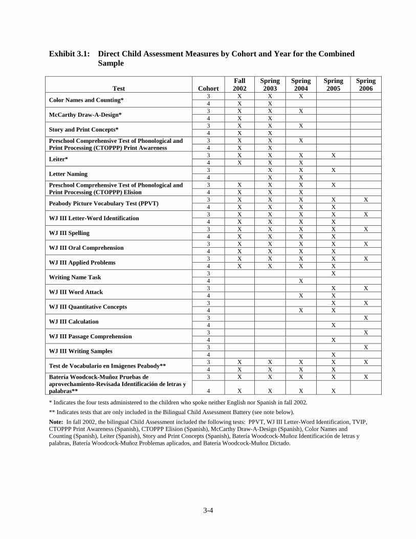
3-4
Exhibit 3.1: Direct Child Assessment Measures by Cohort and Year for the Combined Sample
Test Cohort Fall 2002
Spring 2003
Spring 2004
Spring 2005
Spring 2006
Color Names and Counting* 3 X X X 4 X X
McCarthy Draw-A-Design* 3 X X X 4 X X
Story and Print Concepts* 3 X X X 4 X X
Preschool Comprehensive Test of Phonological and Print Processing (CTOPPP) Print Awareness
3 X X X 4 X X
Leiter* 3 X X X X 4 X X X
Letter Naming 3 X X X 4 X X
Preschool Comprehensive Test of Phonological and Print Processing (CTOPPP) Elision
3 X X X X 4 X X X
Peabody Picture Vocabulary Test (PPVT) 3 X X X X X 4 X X X X
WJ III Letter-Word Identification 3 X X X X X 4 X X X X
WJ III Spelling 3 X X X X X 4 X X X X
WJ III Oral Comprehension 3 X X X X X 4 X X X X
WJ III Applied Problems 3 X X X X X 4 X X X X
Writing Name Task 3 X 4 X
WJ III Word Attack 3 X X 4 X X
WJ III Quantitative Concepts 3 X X 4 X X
WJ III Calculation 3 X 4 X
WJ III Passage Comprehension 3 X 4 X
WJ III Writing Samples 3 X 4 X
Test de Vocabulario en Imágenes Peabody** 3 X X X X X 4 X X X X
Batería Woodcock-Muñoz Pruebas de aprovechamiento-Revisada Identificación de letras y palabras**
3 X X X X X
4 X X X X
* Indicates the four tests administered to the children who spoke neither English nor Spanish in fall 2002. ** Indicates tests that are only included in the Bilingual Child Assessment Battery (see note below). Note: In fall 2002, the bilingual Child Assessment included the following tests: PPVT, WJ III Letter-Word Identification, TVIP, CTOPPP Print Awareness (Spanish), CTOPPP Elision (Spanish), McCarthy Draw-A-Design (Spanish), Color Names and Counting (Spanish), Leiter (Spanish), Story and Print Concepts (Spanish), Batería Woodcock-Muñoz Identificación de letras y palabras, Batería Woodcock-Muñoz Problemas aplicados, and Batería Woodcock-Muñoz Dictado.
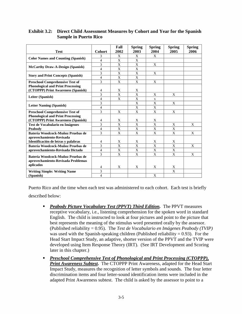
3-5
Exhibit 3.2: Direct Child Assessment Measures by Cohort and Year for the Spanish Sample in Puerto Rico
Test Cohort Fall 2002
Spring 2003
Spring 2004
Spring 2005
Spring 2006
Color Names and Counting (Spanish) 3 X X X 4 X X
McCarthy Draw-A-Design (Spanish) 3 X X X 4 X X
Story and Print Concepts (Spanish) 3 X X X 4 X X
Preschool Comprehensive Test of Phonological and Print Processing (CTOPPP) Print Awareness (Spanish)
3 X X X
4
X
X
Leiter (Spanish) 3 X X X X 4 X X x
Letter Naming (Spanish) 3 X X X 4 X X
Preschool Comprehensive Test of Phonological and Print Processing (CTOPPP) Print Awareness (Spanish)
3 X X X X
4
X
X
X
Test de Vocabulario en Imágenes Peabody
3 X X X X X 4 X X X X
Batería Woodcock-Muñoz Pruebas de aprovechamiento-Revisada Identificación de letras y palabras
3 X X X X X
4
X
X
X
X
Batería Woodcock-Muñoz Pruebas de aprovechamiento-Revisada Dictado
3 X X X X X 4 X X X X
Batería Woodcock-Muñoz Pruebas de aprovechamiento-Revisada Problemas aplicados
3 X X X X X
4
X
X
X
X
Writing Simple: Writing Name (Spanish)
3 X 4 X
Puerto Rico and the time when each test was administered to each cohort. Each test is briefly
described below:
Peabody Picture Vocabulary Test (PPVT) Third Edition. The PPVT measures receptive vocabulary, i.e., listening comprehension for the spoken word in standard English. The child is instructed to look at four pictures and point to the picture that best represents the meaning of the stimulus word presented orally by the assessor. (Published reliability = 0.95). The Test de Vocabulario en Imágenes Peabody (TVIP) was used with the Spanish-speaking children (Published reliability = 0.93). For the Head Start Impact Study, an adaptive, shorter version of the PPVT and the TVIP were developed using Item Response Theory (IRT). (See IRT Development and Scoring later in this chapter.)
Preschool Comprehensive Test of Phonological and Print Processing (CTOPPP), Print Awareness Subtest. The CTOPPP Print Awareness, adapted for the Head Start Impact Study, measures the recognition of letter symbols and sounds. The four letter discrimination items and four letter-sound identification items were included in the adapted Print Awareness subtest. The child is asked by the assessor to point to a

3-6
letter (letter discrimination) and to point to the letter that represents the stimulus sound provided orally by the assessor (letter-sound identification). Print Awareness also measures print concepts, word discrimination, letter-name identification, letter-name identification free response, and letter-sound identification free response. These concepts were eliminated due to overlap with other tests in the child assessment battery. No published reliability is available. The instrument was translated for the Spanish version. The subtest was dropped from the analysis due to poor psychometric properties and difficulty in interpretation of the small number of items.
Preschool Comprehensive Test of Phonological and Print Processing (CTOPPP), Elision Subtest. The CTOPPP Elision measures the ability to remove words, syllables, and sub syllables as part of words or compound words. Both multiple choice and free-response items are included in the subtest. The child is asked to respond by pointing to pictures and to respond verbally to the assessor’s oral directions to make a new word out of words provided (e.g., Say seesaw without see). No published reliability is available. The instrument was translated for the Spanish version.
McCarthy Scales of Children’s Abilities, Draw-A-Design Task. The Draw-A-Design task is a measure of perceptual motor skills. The child is asked to draw a series of increasingly complex figures. The published reliability for the Perceptual-Performance subscale, of which the Draw-A-Design is one component, is 0.84. The task was translated into Spanish for use in the Family and Child Experiences Survey (FACES) for the 1997 cohort and also used in the Head Start Impact Study.
Color Names and Counting. This was a subtest from the CAP (Comprehensive Assessment Program) Early Childhood Diagnostic Instrument used by FACES and developed by Marie Clay (1979), William Teale (1988), and Mason and Stewart (1989) as a battery of emergent literacy and school readiness measures. The subtest measures color recognition (Color Names), and early numeracy skills of counting, and one-to-one correspondence (Counting). The child is asked to identify 10 colors by name and to count 10 pictures of bears and arrive at the correct sum. No published reliability is available. This test was translated into Spanish for use in FACES and also used in the Head Start Impact Study.
Leiter Revised, Sustained Attention Task. This task measures the child’s ability to pay sustained attention to a repetitive task and to pay attention to detail. This is a timed test with a targeted picture at the top of each page. The child is asked to cross as many of the target pictures as possible during the allotted time. The targeted pictures are interspersed among non-target pictures. The Attention Sustained task is one of 10 tasks in the Attention and Memory battery. The overall published reliability is 0.83. The task is a nonverbal task but the directions were translated into Spanish for use in FACES and also used in the Head Start Impact Study. Each task is the same but the targeted pictures become more complex (e.g., from a stick man to a flower) and the matching target and non-target pictures are smaller and more diverse (i.e., more choices, rotated pictures, etc.). During the pilot test, the entire task was administered to the children. It was determined that the task was too long in that the children lost interest early in the task. To lessen the burden, it was decided to use

3-7
only one practice item and one test item for each age cohort. This limitation made it difficult to interpret the scores and thus the Leiter was eliminated from the analysis.
Story and Print Concepts. The Story and Print Concepts task, used in FACES, was based on earlier prereading assessment procedures developed by Marie Clay (1979), William Teale (1988), and Mason and Stewart (1989). This test measures emerging literacy relative to knowledge of books and print concepts. For this test, the assessor asks questions relative to print concepts, such as “Show me the front of the book” and reads passages from a book to the child asking questions as the passage is read, such as “Where do I go next to read?” No published reliability is available. This test was translated into Spanish for use in FACES and also used in the Head Start Impact Study. The books used to assess the child’s story and print concepts were as follows:
o Alborough, J. (1992). Where’s My Teddy? Cambridge, MA: Candlewick Press. (English version)
o Alborough, J. (1995). ¿Dónde Está Mi Osito? (translated by M. Castro) Miami, FL: Santillana USA Publishing Company, Inc. (Spanish version)
To reduce the burden on the child, it was decided to reduce the number of questions from the FACES version. This test was eliminated from the analysis due to the difficulty in scoring the test and interpreting the results.
Letter Naming. This task was modified by the FACES Research Team from a test used in the Head Start Quality Research Center’s (QRC) curricular intervention studies. The Letter Naming task measures the child’s ability to recognize the upper case letters of the alphabet. The letters of the alphabet are divided into three plates with the easiest letters printed on the first plate. Children are asked to identify each letter on the plate. No published reliability is available. This task was translated into Spanish for use in the Head Start Impact Study. Although this task was administered in English to the bilingual children, responses in English or Spanish were acceptable.
Writing Name task. This task was modeled after the Name Writing tasks in The CAP Early Childhood Diagnostic Instrument (Mason and Stewart, 1989) and the Writing Samples test in the Woodcock-Johnson III Tests of Achievement (2001). The task measures the child’s basic writing skills. For this task, the child is asked to write his or her name. No published reliability data is available. This task was translated into Spanish for use in the Head Start Impact Study. Although this test was administered to children at the end of kindergarten, 98 percent of the children could write their name, so the data was not included in the analysis.
Woodcock-Johnson III Tests of Achievement, Letter-Word Identification. The Letter-Word Identification test measures letter and word identification skills. The items measure a child’s reading identification skills in identifying letters and words as they appear in the test easel. The published median reliability is 0.91 in the 5 to 19 age range. The Batería-R Woodcock-Muñoz Pruebas de aprovechamiento-Revisada Identificación de letras y palabras test is used for the Spanish and bilingual test administration.

3-8
Woodcock-Johnson III Tests of Achievement, Spelling. The Spelling test measures the child’s ability to correctly write orally presented letters and words. For the initial items, pre-writing skills are measured through tasks such as drawing lines and copying letters. As the items progress in difficulty, the child is asked to write specific upper and lower cases of the alphabet and specific words. The published median reliability is 0.90 in the 5-19 age range. The Batería-R Woodcock-Muñoz Pruebas de aprovechamiento-Revisada Dictado is used for the Spanish test administration.
Woodcock-Johnson III Tests of Achievement, Applied Problems. This test measures the child’s ability to analyze and solve practical math problems. In order to solve the problems that are read by the assessor to the child, the child must recognize the procedure to be followed and then count and/or perform simple calculations. The published median reliability is 0.92 in the 5-19 age range. The Batería-R Woodcock-Muñoz Pruebas de aprovechamiento-Revisada Problemas aplicados is used for the Spanish test administration.
Woodcock-Johnson III Tests of Achievement, Oral Comprehension. This test measures the child’s ability to comprehend a short spoken passage and to provide a missing word based on syntactic and semantic clues. The test requires the child to use listening, reasoning and vocabulary skills. The assessor reads an analogy or passage with one word missing, the child is asked to respond orally with the correct word that completes the passage or analogy. The published median reliability is 0.80 in the 5-19 age range. No Oral Comprehension test was administered in Spanish.
Woodcock-Johnson III Tests of Achievement, Word Attack. This test measures the child’s ability to apply phonic and structural analysis skills to the pronunciation of printed nonwords. The initial items require the child to produce the sounds for a single letter. The remaining items require the child to read aloud nonwords that become increasingly more difficult. The published median reliability is 0.87 in the 5-19 age range. No Word Attack test was administered in Spanish.
Woodcock-Johnson III Tests of Achievement, Quantitative Concepts. This test consists of two subtests: Concepts and Number Series. Concepts measures the child’s understanding of counting, identifying numbers, shapes and sequences, and knowledge of mathematical terms and formulas. Number Series measures the child’s ability to look at a series of numbers, determine the pattern, and provide the missing number in the series. The published median reliability is 0.90 in the 5-19 age range. No Quantitative Concepts test was administered in Spanish.
Woodcock-Johnson III Tests of Achievement, Calculation. This test measures the ability to perform mathematical computations. The initial items require the child to write single numbers. The items progress in difficulty from basic operations to geometric, trigonometric, logarithmic, and calculus operations. The calculations include operations with whole numbers, percents, fractions, decimals and negative numbers. The published median reliability is 0.85 in the 5-19 age range. No Calculation test was administered in Spanish.
3-9
Woodcock-Johnson III Tests of Achievement, Passage Comprehension. This test measures the child’s ability to match a pictographic representation of a word (rebus) with the actual picture of the object and to read a short passage and identify a missing key word based on the passage context. The items become more difficult by removing pictures and increasing passage length, level of vocabulary, and the complexity of semantic and syntactic clues. The published median reliability is 0.83 in the 5-19 age range. No Passage Comprehension test was administered in Spanish.
Woodcock-Johnson III Tests of Achievement, Writing Samples. This test measures the child’s ability to respond in writing to requests such as completing written passages or writing responses to pictures. The child is asked to respond to simple tasks such as completing the sentence, “My name is __________” to more complex tasks such as writing a sentence to describe a picture (e.g., picture of a bird in a cage singing). The published median reliability is 0.84 in the 5-19 age range. No Writing Samples test was administered in Spanish.
Test Adaptations
Three types of adjustments were made to several tests to significantly reduce the time
required to test individual children (i.e., reducing the burden on the child): (1) adapted or
shortened versions of the PPVT and TVIP were created using item response theory (IRT;
described below); (2) the stopping rules for the Woodcock-Johnson III Tests of Achievement
were changed from six consecutive incorrect responses used in the standard administration of
these tests to three consecutive incorrect responses for determining the ceiling; and (3) only
selected sections or scales were administered for some tests. The first adaptation using IRT
procedures is described in the next section; the remaining adaptations are discussed below.
The stopping rule instructs the assessor when to stop the test because the items have
become too difficult for the child and thus the ceiling is established. The basal items are the
easiest items to be administered while the ceiling items are the most difficult items to be
administered in order to measure the child’s ability in a given cognitive area or construct. This
rule (i.e., three consecutive incorrect responses) was implemented in the FACES child
assessment battery as a means to reduce the time burden on young children with short attention
spans and to reduce the frustration that occurs when a child is asked to answer many difficult
items. This stopping rule was retained in the Head Start Impact Study for comparison purposes.
Changing the stopping rules may result in slightly lower scores when comparing the scores to
normed scores but the same procedures were implemented for both the Head Start and control
group and should not affect the Head Start and control group differences. Due to normal
3-10
cognitive growth and increased attention spans, the standard administration (six consecutive
incorrect responses) was implemented in the first-grade data collection period.
For the Leiter, McCarthy Draw-A-Design and Print Awareness, only selected items,
sections or scales were used to avoid overlap with other tests and to reduce the burden on the
child. The Leiter Attention Sustained Task is one of 10 tasks in the Leiter Attention and
Memory Battery, only one age-appropriate teaching plate and one age-appropriate testing plate
(out of four plates) from the Attention Sustained Task were administered to each child. The
McCarthy Scales of Children’s Abilities consists of 18 subtests organized into six scales (i.e.,
verbal, perceptual performance, quantitative, general cognitive, memory, and motor). The Draw-
A-Design task is one component of the perceptual performance subscale from the McCarthy
Scales of Children’s Abilities and was the scale used in FACES. The CTOPPP Print Awareness
test measures print concepts, letter discrimination, word discrimination, letter-name
identification, and letter-sound identification, only the letter discrimination and letter sound
identification items were included in the child assessment battery.
At the end of each data collection period, the item response patterns were reviewed for
consistency in the administration of stopping rules, ceiling effects, and patterns of non-response.
If problems were identified, the raw data was reviewed for coding or data entry errors. No cases
were eliminated due to such data problems.
IRT Development and Scoring
Introduction
Shortened versions of the PPVT and the TVIP were developed to reduce the testing
burden imposed on the young study children, building on work from the FACES study using a
statistical procedure called maximum likelihood Item Response Theory (IRT).7
IRT has gained
increasing attention in the development of standardized academic tests, particularly when there is
an interest in equating and comparing tests. Some of the issues faced by test developers, and the
solutions that can be addressed through IRT modeling, include the following:
7 There are many books and articles available on the theory and application of IRT. A good reference is:
Hambleton, R.K., Swaminathan, H. & Rogers, H.J. (1991). Fundamentals of Item Response Theory. Newbury Park, CA: Sage Press.
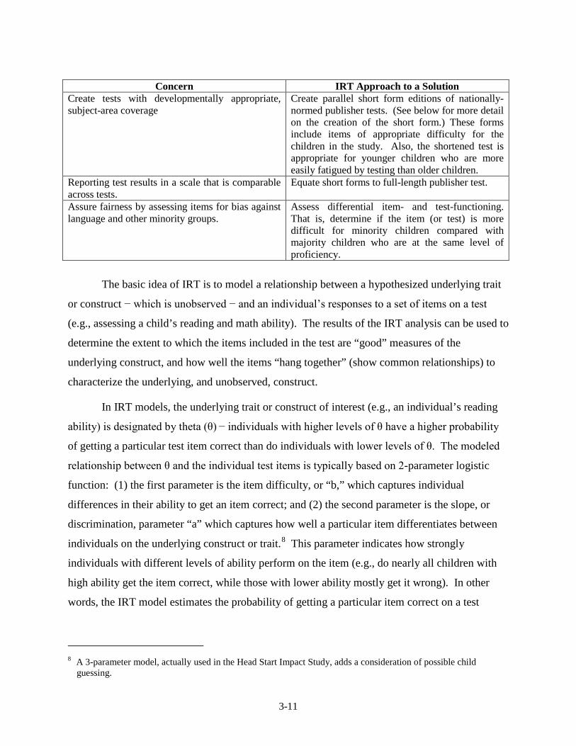
3-11
Concern IRT Approach to a Solution
Create tests with developmentally appropriate, subject-area coverage
Create parallel short form editions of nationally-normed publisher tests. (See below for more detail on the creation of the short form.) These forms include items of appropriate difficulty for the children in the study. Also, the shortened test is appropriate for younger children who are more easily fatigued by testing than older children.
Reporting test results in a scale that is comparable across tests.
Equate short forms to full-length publisher test.
Assure fairness by assessing items for bias against language and other minority groups.
Assess differential item- and test-functioning. That is, determine if the item (or test) is more difficult for minority children compared with majority children who are at the same level of proficiency.
The basic idea of IRT is to model a relationship between a hypothesized underlying trait
or construct − which is unobserved − and an individual’s responses to a set of items on a test
(e.g., assessing a child’s reading and math ability). The results of the IRT analysis can be used to
determine the extent to which the items included in the test are “good” measures of the
underlying construct, and how well the items “hang together” (show common relationships) to
characterize the underlying, and unobserved, construct.
In IRT models, the underlying trait or construct of interest (e.g., an individual’s reading
ability) is designated by theta (θ) − individuals with higher levels of θ have a higher probability
of getting a particular test item correct than do individuals with lower levels of θ. The modeled
relationship between θ and the individual test items is typically based on 2-parameter logistic
function: (1) the first parameter is the item difficulty, or “b,” which captures individual
differences in their ability to get an item correct; and (2) the second parameter is the slope, or
discrimination, parameter “a” which captures how well a particular item differentiates between
individuals on the underlying construct or trait.8
8 A 3-parameter model, actually used in the Head Start Impact Study, adds a consideration of possible child
guessing.
This parameter indicates how strongly
individuals with different levels of ability perform on the item (e.g., do nearly all children with
high ability get the item correct, while those with lower ability mostly get it wrong). In other
words, the IRT model estimates the probability of getting a particular item correct on a test
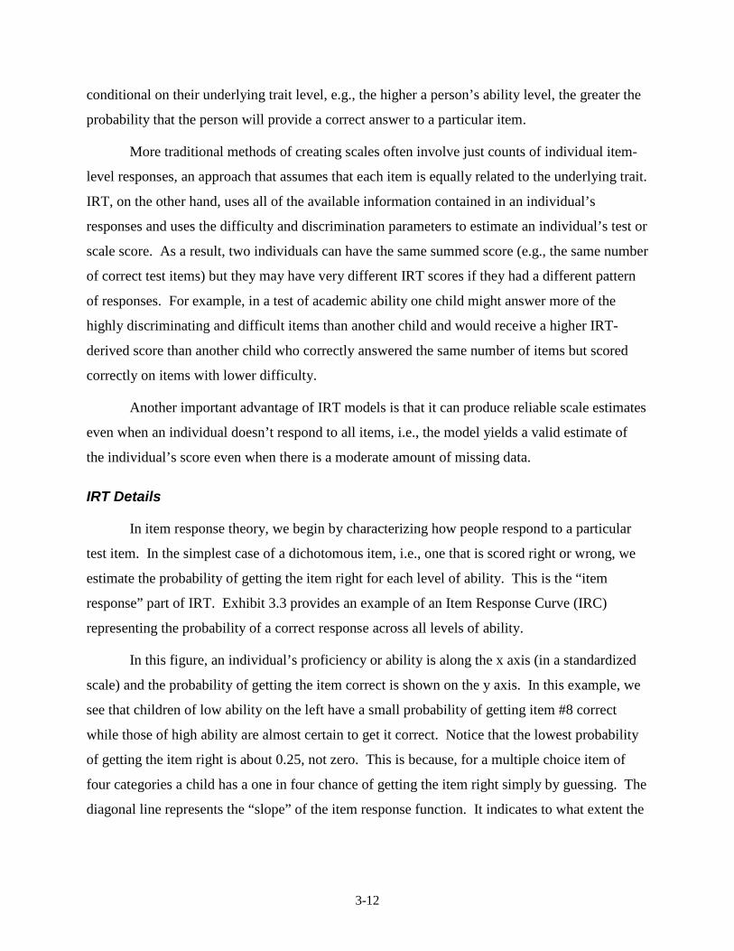
3-12
conditional on their underlying trait level, e.g., the higher a person’s ability level, the greater the
probability that the person will provide a correct answer to a particular item.
More traditional methods of creating scales often involve just counts of individual item-
level responses, an approach that assumes that each item is equally related to the underlying trait.
IRT, on the other hand, uses all of the available information contained in an individual’s
responses and uses the difficulty and discrimination parameters to estimate an individual’s test or
scale score. As a result, two individuals can have the same summed score (e.g., the same number
of correct test items) but they may have very different IRT scores if they had a different pattern
of responses. For example, in a test of academic ability one child might answer more of the
highly discriminating and difficult items than another child and would receive a higher IRT-
derived score than another child who correctly answered the same number of items but scored
correctly on items with lower difficulty.
Another important advantage of IRT models is that it can produce reliable scale estimates
even when an individual doesn’t respond to all items, i.e., the model yields a valid estimate of
the individual’s score even when there is a moderate amount of missing data.
IRT Details
In item response theory, we begin by characterizing how people respond to a particular
test item. In the simplest case of a dichotomous item, i.e., one that is scored right or wrong, we
estimate the probability of getting the item right for each level of ability. This is the “item
response” part of IRT. Exhibit 3.3 provides an example of an Item Response Curve (IRC)
representing the probability of a correct response across all levels of ability.
In this figure, an individual’s proficiency or ability is along the x axis (in a standardized
scale) and the probability of getting the item correct is shown on the y axis. In this example, we
see that children of low ability on the left have a small probability of getting item #8 correct
while those of high ability are almost certain to get it correct. Notice that the lowest probability
of getting the item right is about 0.25, not zero. This is because, for a multiple choice item of
four categories a child has a one in four chance of getting the item right simply by guessing. The
diagonal line represents the “slope” of the item response function. It indicates to what extent the
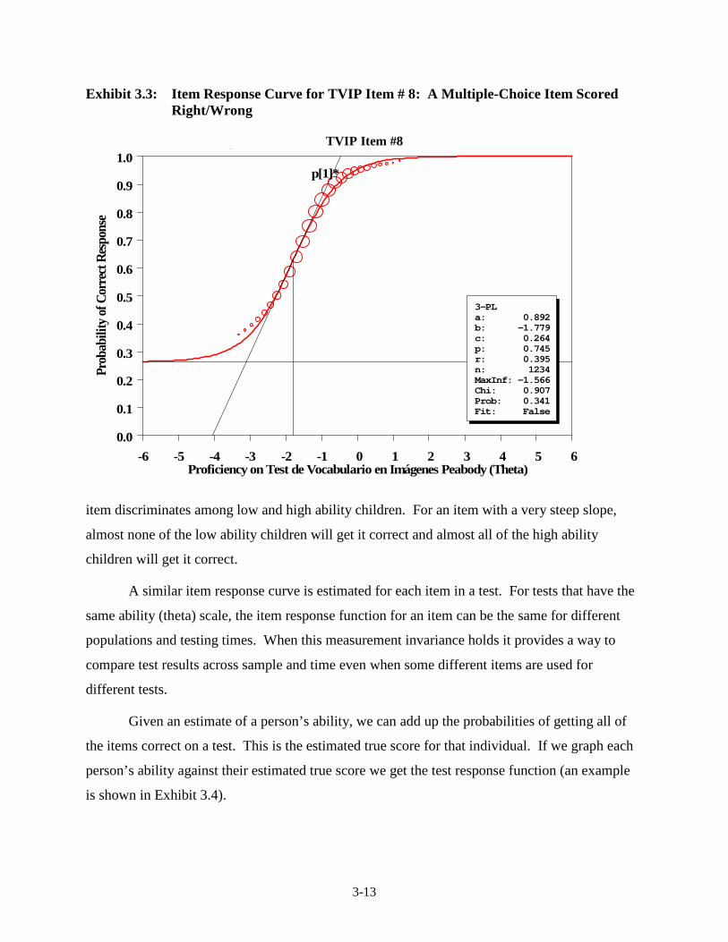
3-13
Exhibit 3.3: Item Response Curve for TVIP Item # 8: A Multiple-Choice Item Scored Right/Wrong
TVIP Item #8
p ( )
Prob
abili
ty of
Cor
rect
Resp
onse
Proficiency on Test de Vocabulario en Imágenes Peabody (Theta)
0.0
0.1
0.2
0.3
0.4
0.5
0.6
0.7
0.8
0.9
1.0
-6 -5 -4 -3 -2 -1 0 1 2 3 4 5 6
p[1]*
3-PLa: 0.892b: -1.779c: 0.264p: 0.745r: 0.395n: 1234MaxInf: -1.566Chi: 0.907Prob: 0.341Fit: False
item discriminates among low and high ability children. For an item with a very steep slope,
almost none of the low ability children will get it correct and almost all of the high ability
children will get it correct.
A similar item response curve is estimated for each item in a test. For tests that have the
same ability (theta) scale, the item response function for an item can be the same for different
populations and testing times. When this measurement invariance holds it provides a way to
compare test results across sample and time even when some different items are used for
different tests.
Given an estimate of a person’s ability, we can add up the probabilities of getting all of
the items correct on a test. This is the estimated true score for that individual. If we graph each
person’s ability against their estimated true score we get the test response function (an example
is shown in Exhibit 3.4).
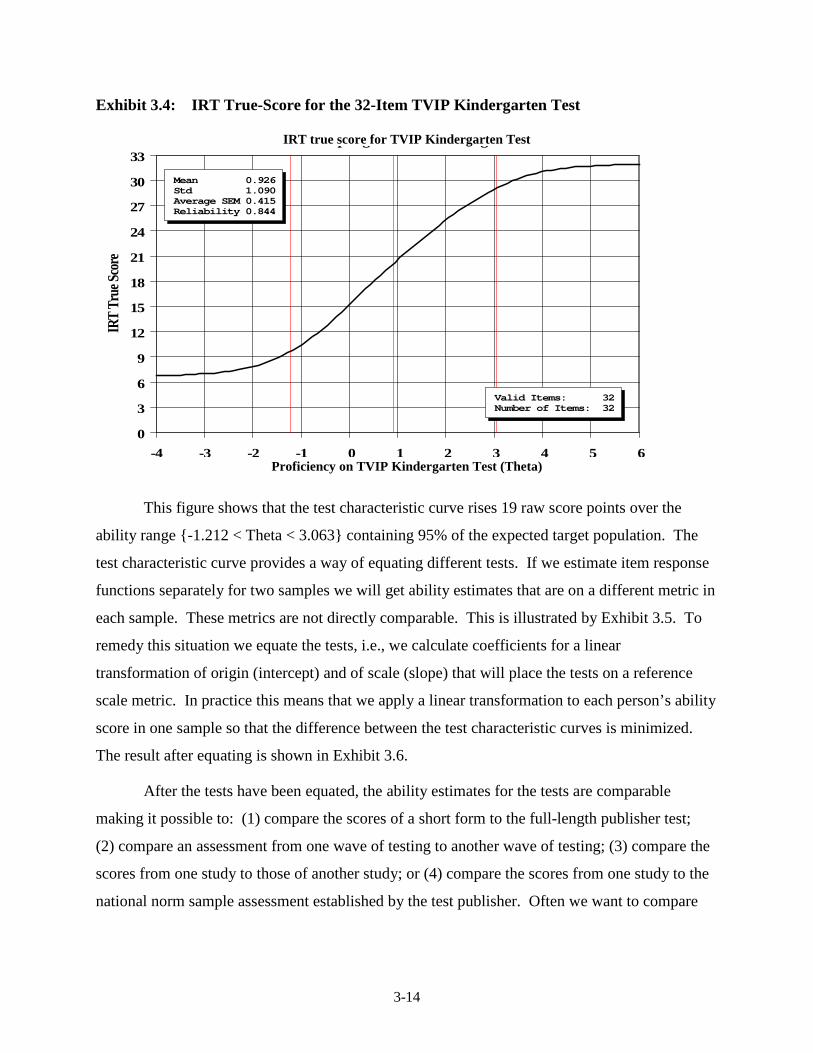
3-14
Exhibit 3.4: IRT True-Score for the 32-Item TVIP Kindergarten Test
IRT true score for TVIP Kindergarten Test
Proficiency on TVIP Kindergarten Test (Theta)
This figure shows that the test characteristic curve rises 19 raw score points over the
ability range {-1.212 < Theta < 3.063} containing 95% of the expected target population. The
test characteristic curve provides a way of equating different tests. If we estimate item response
functions separately for two samples we will get ability estimates that are on a different metric in
each sample. These metrics are not directly comparable. This is illustrated by Exhibit 3.5. To
remedy this situation we equate the tests, i.e., we calculate coefficients for a linear
transformation of origin (intercept) and of scale (slope) that will place the tests on a reference
scale metric. In practice this means that we apply a linear transformation to each person’s ability
score in one sample so that the difference between the test characteristic curves is minimized.
The result after equating is shown in Exhibit 3.6.
After the tests have been equated, the ability estimates for the tests are comparable
making it possible to: (1) compare the scores of a short form to the full-length publisher test;
(2) compare an assessment from one wave of testing to another wave of testing; (3) compare the
scores from one study to those of another study; or (4) compare the scores from one study to the
national norm sample assessment established by the test publisher. Often we want to compare
p g g
IRT
True
Scor
e
0
3
6
9
12
15
18
21
24
27
30
33
-4 -3 -2 -1 0 1 2 3 4 5 6
Mean 0.926Std 1.090Average SEM 0.415Reliability 0.844
Valid Items: 32Number of Items: 32
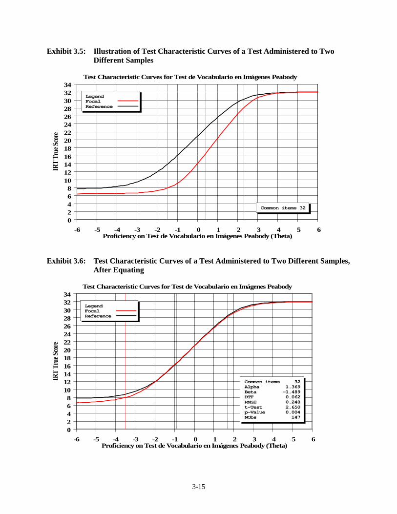
3-15
Exhibit 3.5: Illustration of Test Characteristic Curves of a Test Administered to Two Different Samples
Exhibit 3.6: Test Characteristic Curves of a Test Administered to Two Different Samples,
After Equating
Test Characteristic Curves for Test de Vocabulario en Imágenes Peabody
IRT
True
Scor
e
Proficiency on Test de Vocabulario en Imágenes Peabody (Theta)
0 2 4 6 810121416182022242628303234
-6 -5 -4 -3 -2 -1 0 1 2 3 4 5 6
Common items 32
LegendFocalReference
Test Characteristic Curves for Test de Vocabulario en Imágenes Peabody
IRT
True
Scor
e
Proficiency on Test de Vocabulario en Imágenes Peabody (Theta)
0 2 4 6 810121416182022242628303234
-6 -5 -4 -3 -2 -1 0 1 2 3 4 5 6
Common items 32Alpha 1.369Beta -1.489DTF 0.062RMSE 0.248t-Test 2.650p-Value 0.004NObs 147
LegendFocalReference
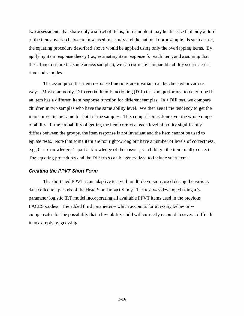
3-16
two assessments that share only a subset of items, for example it may be the case that only a third
of the items overlap between those used in a study and the national norm sample. Is such a case,
the equating procedure described above would be applied using only the overlapping items. By
applying item response theory (i.e., estimating item response for each item, and assuming that
these functions are the same across samples), we can estimate comparable ability scores across
time and samples.
The assumption that item response functions are invariant can be checked in various
ways. Most commonly, Differential Item Functioning (DIF) tests are performed to determine if
an item has a different item response function for different samples. In a DIF test, we compare
children in two samples who have the same ability level. We then see if the tendency to get the
item correct is the same for both of the samples. This comparison is done over the whole range
of ability. If the probability of getting the item correct at each level of ability significantly
differs between the groups, the item response is not invariant and the item cannot be used to
equate tests. Note that some item are not right/wrong but have a number of levels of correctness,
e.g., 0=no knowledge, 1=partial knowledge of the answer, 3= child got the item totally correct.
The equating procedures and the DIF tests can be generalized to include such items.
Creating the PPVT Short Form
The shortened PPVT is an adaptive test with multiple versions used during the various
data collection periods of the Head Start Impact Study. The test was developed using a 3-
parameter logistic IRT model incorporating all available PPVT items used in the previous
FACES studies. The added third parameter – which accounts for guessing behavior --
compensates for the possibility that a low-ability child will correctly respond to several difficult
items simply by guessing.

3-17
The adaptive short form was created by selecting items of appropriate difficulty for the
fall 2002 and spring 2003 Head Start Impact Study test administrations. The appropriate
difficulty level was determined by examining the latent ability distribution of children of similar
ages to the Head Start study sample who were included in FACES.9
The adapted test consists of a 20-item “core” set of test items that is used as a router test
in all test versions: (a) if a child had 11 or fewer core items correct, they were administered the
“basal item” set; (b) if a child had 17 or more core items correct they were administered the
“ceiling item” set; and, (c) if a child had between 11 and 17 items right, no further items were
administered (i.e., their score was based on the core set of items. Three versions of the adapted
test were developed: in Version 1, the ceiling and basal sets each had 10 items, while in
Versions 2 and 3, the basal and ceiling item sets each had nine items.
Versions 1 and 3 were comprised of odd-numbered items taken from the original PPVT,
while Version 2 included only even-numbered items taken from the original PPVT. As a result
Version 2 has no overlap with the other versions. There are 31 items that overlap between
Versions 1 and 3 (a 77% overlap). The new items introduced in Version 3 were all in the ceiling
set. Because there are no common items linking the three different PPVT adapted short forms,
the earlier FACES calibrations serve as an external anchor test. That is, each of the three
adapted PPVT test versions was equated to the FACES standard, placing all scores on a
consistent scale metric (see previous discussion). After equating, the Head Start adapted PPVT
tests were rescaled to all have a mean of 250 and a standard deviation of 50 in the base year (i.e.,
fall 2002). The following exhibit documents the versions used in each test administration.
Exhibit 3.7: PPVT Version Used by Cohort and Data Collection Wave Cohort Fall 2002 Spring 2003 Spring 2004 Spring 2005 Spring 2006 3-year-olds Version 1
(pre-K) Version 1 (pre-K)
Version 2 (pre-K)
Version 3 (K)
Version 3 (1st grade)
4-year-olds Version 1 (pre-K)
Version 1 (pre-K)
Version 2 (K)
Version 3 (1st grade)
9 In FACES, a model-based estimate of the raw score was calculated by summing the probabilities of a correct
response across all items at a given ability level. Unlike the scoring algorithms employed by the testing company, there is no assumption that easier items not presented are correct or that harder items not reached are incorrect. Such strong assumptions about how the child would have done on items they didn’t take may lead to inaccurate estimates of an individual’s ability.
3-18
Scoring the Adapted PPVT Test
Scoring individual child tests was done separately by age cohorts. This guarantees that
the estimates of the age cohort ability distributions are unbiased estimates for each individual
cohort. Within each age cohort, an individual child’s ability score was based on his/her actual
pattern of right, wrong, and omitted responses to the administered test items to place each child
on a continuous scale defined by the IRT item difficulty, discrimination and guessing behavioral
parameters. The scoring procedure used a marginal maximum likelihood approach to correctly
estimate the IRT item parameters (Mislevy & Bock, 1983).
Under marginal maximum likelihood estimation, an individual’s ability score is based on
two types of information: (1) a “prior distribution”, discussed below, for each child, i.e., an
estimate of what scores would look like in the absence of any data (e.g., if one were trying to
estimate tomorrow’s temperature a good “prior” would be today’s temperature); and (2) how an
individual child performed on the administered test. That is, an individual child’s ability score −
referred to as the expected a posteriori (EAP) estimate − is based on a combination of the
estimated prior and his/her actual pattern of test score responses. The greater the reliability of
the test, the more an individual’s actual test responses determines his/her EAP ability score; for
tests that are more unreliable the more the estimated prior will determine the ability score. In
effect ability scores are “shrunken” towards the prior mean in proportion to the reliability of the
test.
The most common approach for creating an assumption for the prior is to assume a single
prior distribution for all children. However, when subgroups of children are being compared −
in this case, a comparison between the children assigned to the Head Start group and those
assigned to the control group − using a separate prior distribution for each subgroup produces
less biased estimates of Head Start/control group means and standard deviations and of any
differences between the two groups (Mislevy, 1991). As a consequence, within each age cohort
(i.e., separately for children in the 3- and 4-year-old cohorts) separate prior distributions were
estimated for Head Start and control group children.
The prior distributions were estimated from the actual test responses (for each separate
wave of data collection) by accumulating individual likelihood distributions (estimated for each
child) to obtain marginal likelihood distributions separately for the Head Start and control

3-19
groups, in each of the two age cohorts. These estimated marginal distributions then served as the
prior distributions used in the calculation of ability scores for each individual child. As a result,
the “shrinkage” of the scores is toward the mean for each random assignment group rather than
to the grand mean of all children.
Changes in Scoring from the Interim Report: It should be noted that the IRT approach
used in the First Year Report was slightly different from that described here and used in the Final
Report. The IRT approach used in the HSIS is called marginal maximum likelihood (or MML).
The MML approach yields consistent estimates of item parameters. Also, in contrast to other
IRT procedures, it yields plausible estimates of ability when a child gets all or none of the items
correct (Mislevy & Bock, 1983). However, to use MML IRT, the analyst must posit the
distribution of the child’s ability prior to testing by estimating the distribution of ability for the
demographic group of the child. This is called the prior distribution of the child’s ability. The
final estimate of a particular child’s ability uses information from the prior guess of the child’s
ability together with the information derived from how the child responded to the current
assessment. Commonly a single prior distribution is assumed for all examinees, which was what
was done for the First Year Report.
For the current report, however, it was decided that a more valid estimate of Head Start
and control group differences could be generated if a separate prior distribution was assumed for
children in the Head Start group and for children in the control group. When children come from
more than one population and comparisons are to be made between the estimated population
means, an unbiased estimate of group differences can be obtained by allowing for potentially
different prior distributions for the two groups being compared (Mislevy, 1991). If separate prior
differences are not assumed for the two groups the IRT group means will tend to be “shrunken”
towards the grand mean, resulting in Head Start-control group differences that are too small.
This would have the effect of biasing downward all IRT-based impact estimates and decreasing
the power to detect treatment effects when they exist. As a result of these considerations, IRT
scaling was implemented for this report assuming separate prior distributions for the Head Start
and control groups. This leads to results for the PPVT and TVIP in spring 2003 that will be
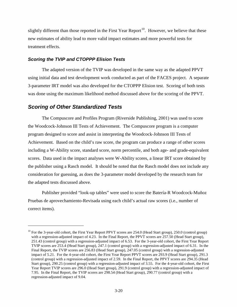
3-20
slightly different than those reported in the First Year Report10
Scoring the TVIP and CTOPPP Elision Tests
. However, we believe that these
new estimates of ability lead to more valid impact estimates and more powerful tests for
treatment effects.
The adapted version of the TVIP was developed in the same way as the adapted PPVT
using initial data and test development work conducted as part of the FACES project. A separate
3-parameter IRT model was also developed for the CTOPPP Elision test. Scoring of both tests
was done using the maximum likelihood method discussed above for the scoring of the PPVT.
Scoring of Other Standardized Tests
The Compuscore and Profiles Program (Riverside Publishing, 2001) was used to score
the Woodcock-Johnson III Tests of Achievement. The Compuscore program is a computer
program designed to score and assist in interpreting the Woodcock-Johnson III Tests of
Achievement. Based on the child’s raw score, the program can produce a range of other scores
including a W-Ability score, standard score, norm percentile, and both age- and grade-equivalent
scores. Data used in the impact analyses were W-Ability scores, a linear IRT score obtained by
the publisher using a Rasch model. It should be noted that the Rasch model does not include any
consideration for guessing, as does the 3-parameter model developed by the research team for
the adapted tests discussed above.
Publisher provided “look-up tables” were used to score the Batería-R Woodcock-Muñoz
Pruebas de aprovechamiento-Revisada using each child’s actual raw scores (i.e., number of
correct items).
10 For the 3-year-old cohort, the First Year Report PPVT scores are 254.0 (Head Start group), 250.0 (control group)
with a regression-adjusted impact of 4.23. In the Final Report, the PPVT scores are 257.50 (Head Start group), 251.43 (control group) with a regression-adjusted impact of 6.53. For the 3-year-old cohort, the First Year Report TVIP scores are 253.4 (Head Start group), 247.1 (control group) with a regression-adjusted impact of 6.31. In the Final Report, the TVIP scores are 256.83 (Head Start group), 247.05 (control group) with a regression-adjusted impact of 5.21. For the 4-year-old cohort, the First Year Report PPVT scores are 293.9 (Head Start group), 291.3 (control group) with a regression-adjusted impact of 2.59. In the Final Report, the PPVT scores are 294.35 (Head Start group), 290.25 (control group) with a regression-adjusted impact of 3.55. For the 4-year-old cohort, the First Year Report TVIP scores are 296.0 (Head Start group), 291.9 (control group) with a regression-adjusted impact of 7.95. In the Final Report, the TVIP scores are 298.54 (Head Start group), 290.77 (control group) with a regression-adjusted impact of 9.04.
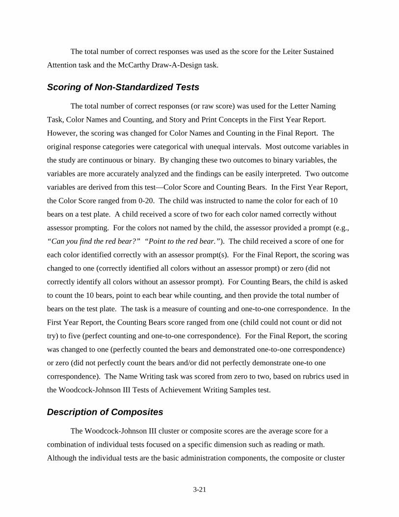
3-21
The total number of correct responses was used as the score for the Leiter Sustained
Attention task and the McCarthy Draw-A-Design task.
Scoring of Non-Standardized Tests
The total number of correct responses (or raw score) was used for the Letter Naming
Task, Color Names and Counting, and Story and Print Concepts in the First Year Report.
However, the scoring was changed for Color Names and Counting in the Final Report. The
original response categories were categorical with unequal intervals. Most outcome variables in
the study are continuous or binary. By changing these two outcomes to binary variables, the
variables are more accurately analyzed and the findings can be easily interpreted. Two outcome
variables are derived from this test—Color Score and Counting Bears. In the First Year Report,
the Color Score ranged from 0-20. The child was instructed to name the color for each of 10
bears on a test plate. A child received a score of two for each color named correctly without
assessor prompting. For the colors not named by the child, the assessor provided a prompt (e.g.,
“Can you find the red bear?” “Point to the red bear.”). The child received a score of one for
each color identified correctly with an assessor prompt(s). For the Final Report, the scoring was
changed to one (correctly identified all colors without an assessor prompt) or zero (did not
correctly identify all colors without an assessor prompt). For Counting Bears, the child is asked
to count the 10 bears, point to each bear while counting, and then provide the total number of
bears on the test plate. The task is a measure of counting and one-to-one correspondence. In the
First Year Report, the Counting Bears score ranged from one (child could not count or did not
try) to five (perfect counting and one-to-one correspondence). For the Final Report, the scoring
was changed to one (perfectly counted the bears and demonstrated one-to-one correspondence)
or zero (did not perfectly count the bears and/or did not perfectly demonstrate one-to one
correspondence). The Name Writing task was scored from zero to two, based on rubrics used in
the Woodcock-Johnson III Tests of Achievement Writing Samples test.
Description of Composites
The Woodcock-Johnson III cluster or composite scores are the average score for a
combination of individual tests focused on a specific dimension such as reading or math.
Although the individual tests are the basic administration components, the composite or cluster

3-22
interpretation minimizes the potential problem of generalizing from the score for a single, narrow
ability to a broad, multifaceted domain and provides higher validity because more than one score
serves as the basis for the interpretation of a child’s ability (Mather and Woodcock, 2001). The
child’s performance on an individual test informs the broader measure of general ability in the
composite or cluster score. The composite scores developed by Woodcock-Johnson III are based
on developmental evidence from research on children’s growth patterns. Composite scores from
the Woodcock-Johnson III that are used in the study include the following:
Pre-Academic Cluster. This cluster provides an early overall academic measure including pre-reading and letter and word identification skills, developing mathematics skills, and early writing and spelling skills. Tests included in the cluster include Letter-Word Identification, Spelling, and Applied Problems. The reliability is 0.97 for four- and five-year olds and 0.98 for six year olds. A similar cluster (Skills Cluster) is available for the Spanish assessment in Puerto Rico.
Basic Reading Skills. This cluster provides an overall measure of basic reading skills including sight vocabulary, phonics, and structural analysis. Tests included in the cluster are Letter-Word Identification and Word Attack. The published median reliability is 0.93 in the 5-19 age range. An equivalent composite is not available for the Spanish assessment in Puerto Rico.
Math Reasoning. This cluster provides an overall measure of mathematical knowledge and reasoning including mathematical problem solving and vocabulary and analysis. Tests included in the cluster are Applied Problems and Quantitative Concepts. The published median reliability is 0.95 in the 5-19 age range. An equivalent composite is not available for the Spanish assessment in Puerto Rico.
Academic Skills. This cluster provides an overall score of basic achievement skills including reading, math calculation, and spelling. Tests included in the cluster are Letter-Word Identification, Calculation, and Spelling. The published median reliability is 0.95 in the 5-19 age range. An equivalent composite is not available for the Spanish assessment in Puerto Rico.
Academic Applications. This cluster measures the application of academic skills to academic problems. Tests included in the cluster are Passage Comprehension, Applied Problems, and Writing Samples. The published median reliability is 0.94 in the 5-19 age range. An equivalent composite is not available for the Spanish assessment in Puerto Rico.
Exhibit 3.8 provides the list of composites and the time when the necessary scales comprising
each composite were available for each cohort in the combined sample. As noted above, only
the Skills Composite is available for the Spanish assessment.
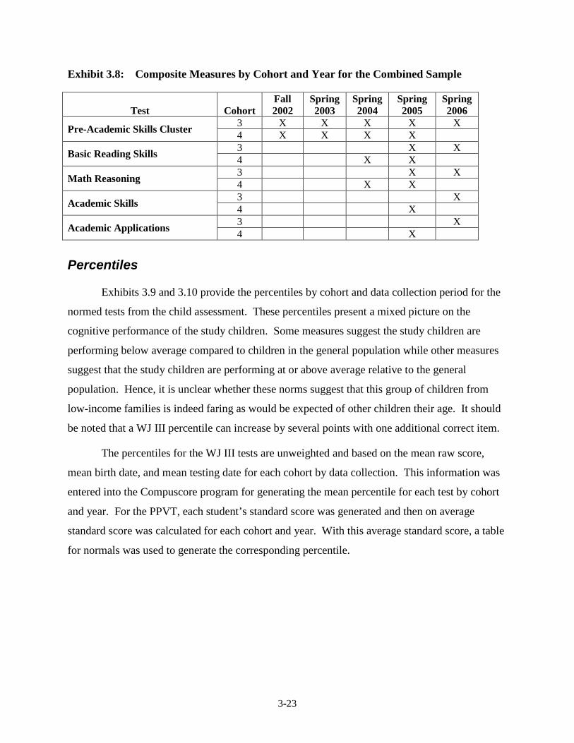
3-23
Exhibit 3.8: Composite Measures by Cohort and Year for the Combined Sample
Test Cohort Fall 2002
Spring 2003
Spring 2004
Spring 2005
Spring 2006
Pre-Academic Skills Cluster 3 X X X X X 4 X X X X
Basic Reading Skills 3 X X 4 X X
Math Reasoning 3 X X 4 X X
Academic Skills 3 X 4 X
Academic Applications 3 X 4 X
Percentiles
Exhibits 3.9 and 3.10 provide the percentiles by cohort and data collection period for the
normed tests from the child assessment. These percentiles present a mixed picture on the
cognitive performance of the study children. Some measures suggest the study children are
performing below average compared to children in the general population while other measures
suggest that the study children are performing at or above average relative to the general
population. Hence, it is unclear whether these norms suggest that this group of children from
low-income families is indeed faring as would be expected of other children their age. It should
be noted that a WJ III percentile can increase by several points with one additional correct item.
The percentiles for the WJ III tests are unweighted and based on the mean raw score,
mean birth date, and mean testing date for each cohort by data collection. This information was
entered into the Compuscore program for generating the mean percentile for each test by cohort
and year. For the PPVT, each student’s standard score was generated and then on average
standard score was calculated for each cohort and year. With this average standard score, a table
for normals was used to generate the corresponding percentile.
3-24
Exhibit 3.9: Percentiles on the Norm-Referenced Tests for the 4-Year-Old Cohort by Year
Test
Fall 2002 Baseline
Spring 2003 Head Start
Spring 2004 Kindergarten
Spring 2005 1st Grade
Head Start Group
Control Group
Head Start Group
Control Group
Head Start Group
Control Group
Head Start Group
Control Group
Language and Literacy PPVT (Adapted) 29 28 31 27 28 26 28 25 WJ III Letter-Word Identification 34 34 46 38 62 62 63 63 WJ III Spelling 34 34 30 30 58 58 61 61 WJ III Oral Comprehension 39 38 29 29 33 40 42 42 WJ III Pre-Academic Skills 40 31 32 30 54 54 60 60 WJ III Word Attack -- -- -- -- 93 93 81 81 WJ III Basic Reading Skills -- -- -- -- 82 82 73 73 WJ III Academic Applications -- -- -- -- -- -- 42 42 WJ III Academic Skills -- -- -- -- -- -- 65 65 WJ III Passage Comprehension -- -- -- -- -- -- 38 38 WJ III Writing Samples -- -- -- -- -- -- 46 46
Math WJ III Applied Problems 30 30 23 23 36 36 47 47 WJ III Quantitative Concepts -- -- -- -- 43 43 38 38 WJ III Math Reasoning -- -- -- -- 36 36 42 42 WJ III Calculation -- -- -- -- -- -- 62 62
NOTE: --indicates data not collected on the outcome for the cohort during the data collection period.
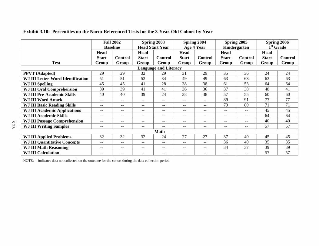
3-25
Exhibit 3.10: Percentiles on the Norm-Referenced Tests for the 3-Year-Old Cohort by Year
Test
Fall 2002 Baseline
Spring 2003 Head Start Year
Spring 2004 Age 4 Year
Spring 2005 Kindergarten
Spring 2006 1st Grade
Head Start
Group Control Group
Head Start
Group Control Group
Head Start
Group Control Group
Head Start
Group Control Group
Head Start
Group Control Group
Language and Literacy PPVT (Adapted) 29 29 32 29 31 29 35 36 24 24 WJ III Letter-Word Identification 51 51 52 34 49 49 63 63 63 63 WJ III Spelling 45 45 41 28 38 38 61 53 64 64 WJ III Oral Comprehension 39 39 41 41 36 36 37 38 48 41 WJ III Pre-Academic Skills 40 40 39 24 38 38 57 55 60 60 WJ III Word Attack -- -- -- -- -- -- 89 91 77 77 WJ III Basic Reading Skills -- -- -- -- -- -- 79 80 71 71 WJ III Academic Applications -- -- -- -- -- -- -- -- 45 45 WJ III Academic Skills -- -- -- -- -- -- -- -- 64 64 WJ III Passage Comprehension -- -- -- -- -- -- -- -- 40 40 WJ III Writing Samples -- -- -- -- -- -- -- -- 57 57
Math WJ III Applied Problems 32 32 32 24 27 27 37 40 45 45 WJ III Quantitative Concepts -- -- -- -- -- -- 36 40 35 35 WJ III Math Reasoning -- -- -- -- -- -- 34 37 39 39 WJ III Calculation -- -- -- -- -- -- -- -- 57 57
NOTE: --indicates data not collected on the outcome for the cohort during the data collection period.

3-26
Other Cognitive Outcomes
The tests included in the direct child assessment battery are described above. Other
measures of children’s cognitive skills include the following:
Teacher report of academic skills. Each child is rated on three academic skills (language and literacy, science and social studies, and mathematical skills) by his/her teacher. The child is rated as compared to other children at the same grade level using a five point scale ranging from one (far below average) to five (far above average).
Teacher report of school accomplishments. Each child is rated by his/her teacher on a series of items that describe the child’s skills, knowledge, and behaviors focusing on language and literacy and mathematics. The child is rated using a five point scale that reflects the degree to which the child has acquired the demonstrated skills, knowledge, and behaviors ranging from one (not yet) to five (proficient). More complex skills, knowledge, and behaviors are added to the first grade list.
Parent report of promotion. Parents were asked the grade level of their child. This information was confirmed with the teacher-reported expected promotion of the child. Overall there was consistency between the two reports. Parent data were used because the response rate was higher for parents than teachers and it provided the actual promotion data while the teacher data provided information on whether or not the child was expected to be promoted to the next grade.
Parent emergent literacy scale (PELS). PELS is a parent-report on five literacy items originally developed for use in FACES 2000: child can recognize most/all of the letters of the alphabet; child can count to 20; child pretended to write his/her name in the last month; child can write his/her first name; and child can identify the primary colors.
Social-Emotional Outcomes
Social skills and positive approaches to learning. Parents are asked to rate their child’s social skills and positive approaches to learning. The measure assesses social skills focused on cooperative and empathic behavior, such as, "Makes friends easily," "Comforts or helps others," and "Accepts friends' ideas in sharing and playing.” The measure also assesses aspects of children’s approaches to learning such as curiosity, imagination, openness to new tasks and challenges, and having a positive attitude about gaining new knowledge and skills. Examples include, "Enjoys learning," "Likes to try new things," and "Shows imagination in work and play.” The scale contains seven items, with each item scored from zero (not true) to two (very true), and the scale scores can range from 0 to 14. The scale is based on an instrument used in the Head Start Family and Child Experiences Survey (FACES).11
11 Administration on Children and Families (2001). Retrieved 10/15/04 from:
http://www.acf.dhhs.gov/programs/core/ongoing_research/faces/faces_instruments.html
Mean scores on the scale obtained from parents of Head Start children in the Head Start Impact Study
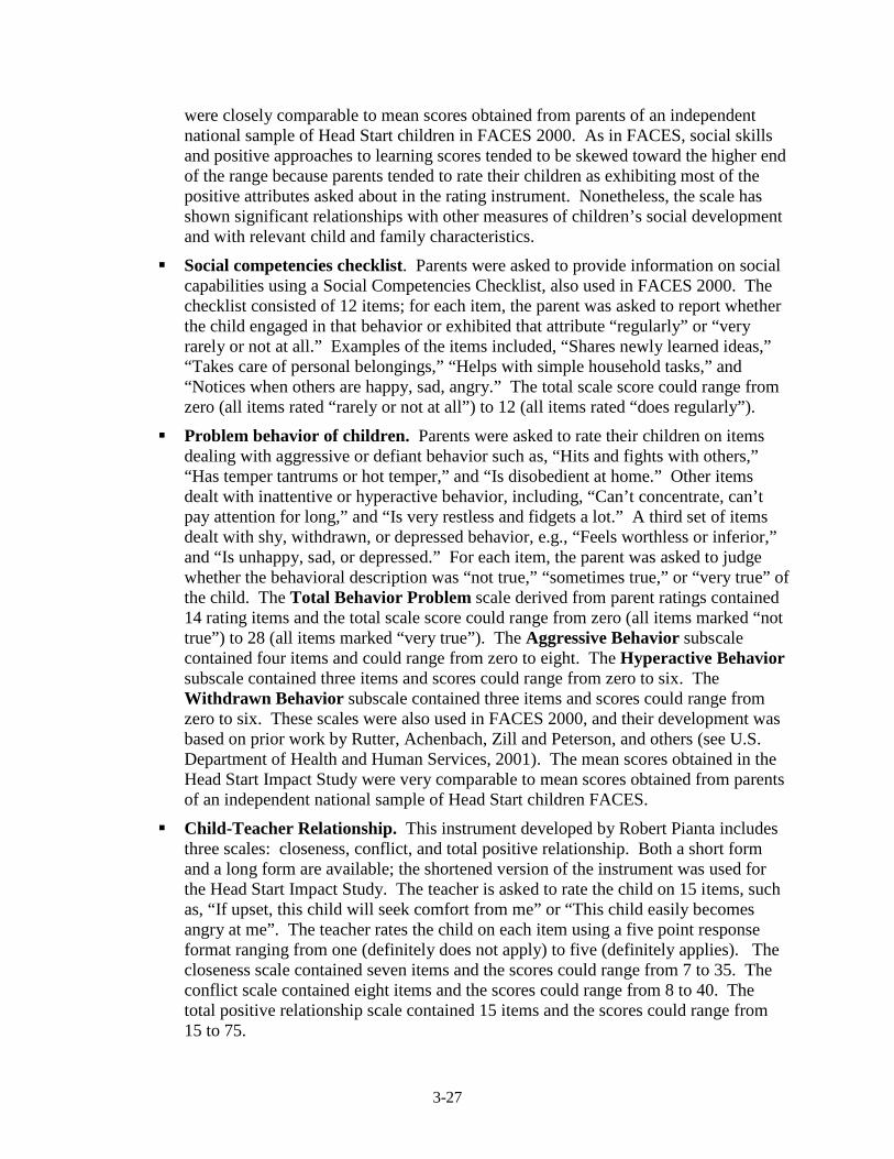
3-27
were closely comparable to mean scores obtained from parents of an independent national sample of Head Start children in FACES 2000. As in FACES, social skills and positive approaches to learning scores tended to be skewed toward the higher end of the range because parents tended to rate their children as exhibiting most of the positive attributes asked about in the rating instrument. Nonetheless, the scale has shown significant relationships with other measures of children’s social development and with relevant child and family characteristics.
Social competencies checklist. Parents were asked to provide information on social capabilities using a Social Competencies Checklist, also used in FACES 2000. The checklist consisted of 12 items; for each item, the parent was asked to report whether the child engaged in that behavior or exhibited that attribute “regularly” or “very rarely or not at all.” Examples of the items included, “Shares newly learned ideas,” “Takes care of personal belongings,” “Helps with simple household tasks,” and “Notices when others are happy, sad, angry.” The total scale score could range from zero (all items rated “rarely or not at all”) to 12 (all items rated “does regularly”).
Problem behavior of children. Parents were asked to rate their children on items dealing with aggressive or defiant behavior such as, “Hits and fights with others,” “Has temper tantrums or hot temper,” and “Is disobedient at home.” Other items dealt with inattentive or hyperactive behavior, including, “Can’t concentrate, can’t pay attention for long,” and “Is very restless and fidgets a lot.” A third set of items dealt with shy, withdrawn, or depressed behavior, e.g., “Feels worthless or inferior,” and “Is unhappy, sad, or depressed.” For each item, the parent was asked to judge whether the behavioral description was “not true,” “sometimes true,” or “very true” of the child. The Total Behavior Problem scale derived from parent ratings contained 14 rating items and the total scale score could range from zero (all items marked “not true”) to 28 (all items marked “very true”). The Aggressive Behavior subscale contained four items and could range from zero to eight. The Hyperactive Behavior subscale contained three items and scores could range from zero to six. The Withdrawn Behavior subscale contained three items and scores could range from zero to six. These scales were also used in FACES 2000, and their development was based on prior work by Rutter, Achenbach, Zill and Peterson, and others (see U.S. Department of Health and Human Services, 2001). The mean scores obtained in the Head Start Impact Study were very comparable to mean scores obtained from parents of an independent national sample of Head Start children FACES.
Child-Teacher Relationship. This instrument developed by Robert Pianta includes three scales: closeness, conflict, and total positive relationship. Both a short form and a long form are available; the shortened version of the instrument was used for the Head Start Impact Study. The teacher is asked to rate the child on 15 items, such as, “If upset, this child will seek comfort from me” or “This child easily becomes angry at me”. The teacher rates the child on each item using a five point response format ranging from one (definitely does not apply) to five (definitely applies). The closeness scale contained seven items and the scores could range from 7 to 35. The conflict scale contained eight items and the scores could range from 8 to 40. The total positive relationship scale contained 15 items and the scores could range from 15 to 75.

3-28
Child-Parent Relationship. Parents were asked to rate their child’s relationship with them. The same scales and scoring were used as described for the Child Teacher Relationship scale. It also should be noted that he long version of the Child Teacher Relationship was adapted for use with parents in The NICHD Study of Early Child Care.
Adjustment Scales for Preschool Intervention (ASPI). The ASPI is based on the ASCA (Adjustment Scales for Children and Adolescents). The ASPI (Lutz, Fantuzzo, & McDermott, 2002) contains 24 classroom situations that provide 144 descriptors of both typical and problem classroom behavior. The teacher is asked to select all behavior descriptions that match a child’s behavior to a specified classroom situation over the past two months. For example, one classroom situation is, “How does this child seek your help?” The behavior descriptions are: too lethargic to ask, asks for help when needed, seeks help when not needed, rarely needs help, not shy but never seeks help, or too timid to ask. The teacher is instructed to select any behavior description that she/he observed for this child during the past two months. The factors identified from the ASPI are aggressive, withdrawn/low energy, socially reticent, oppositional, and inattentive/hyperactive. In addition, three situational dimensions have been identified with the ASPI—structured learning, peer interaction, and teacher interaction. The raw score is based on the sum of the checked behavior descriptions for the items that loaded on each factor and the raw scores are converted to t-scores derived from the developer’s original ASPI standardization sample.
Health Outcomes
Receipt of health care services. Parents were asked to report on various health care services, two of which are used in this report: o Whether the child has health insurance. Parents were asked if the child was
currently covered by Medicaid or a state health insurance program, or by health insurance through their job or the job of another employed adult.
o Whether the child has received dental care. Parents were asked if the child had ever seen a dentist since September of that year.12
Child’s health status. Parents were asked to report on their child’s health status:
o Child’s health status (excellent or very good). Parents were asked if, overall, the child’s health was excellent, very good, good, fair, or poor. This outcome was coded “yes” for those who reported that their child’s health was excellent or very good.
o Whether the child needs ongoing medical care. Parents were asked if their child had an illness or condition that requires regular ongoing medical care.
o Whether child received medical care for an injury in the last month. Parents were asked how many times their child, in the last month, had seen a doctor or other medical professional or visited a clinic or emergency room for an injury.
12 At the time of the 2002 baseline, parents were asked whether the child had seen a dentist.

3-29
This outcome was coded yes if the parent reported any such occurrences in the last month.
Parenting Outcomes
Educational activities. Parents were asked to report on the types of educational activities they did with their child:
o Reading to the child at home. Parents reported on the item “How many times have you or someone in your family read to [CHILD] in the past week?” Possible responses range from one (not at all) to four (every day).
o Family cultural enrichment activities. Parents reported on a seven-item checklist of activities the parent, or another family member, may have done with the child during the past month. The seven activities include going to a movie; play or concert; art gallery or museum; playground, park, or zoo; community, ethnic, or religious event; and talking about family or cultural heritage and going on errands. A total score was computed by summing the number of different activities the parent and child participated in together, with a possible score of zero (none) to seven (all).
Discipline practices. Parents reported on the following:
o Use of physical discipline. Parents reported on the item “Sometimes children mind pretty well and sometimes they don’t. Have you spanked [CHILD] in the past week for not minding?”
o Use of time out. Parents reported on the item “Have you used ‘time out’ or sent [CHILD] to his/her room in the past week for not minding?”
Parental safety practices. Parents reported on a 10-item scale that assessed how often the 10 different safety precautions were used, including keeping harmful objects out of reach, using car seats, supervising the child during bath time, and having a first aid kit and working smoke detector at home. Possible responses ranged from one (never) to four (always).
Parenting styles. The parents were asked to respond to selected items from the Child –Rearing Practices Report (CRPR) (Block, 1965). Parents were asked to respond to items, such as, “I teach my child that misbehavior or breaking the rules will always be punished one way or another” and “I believe physical punishment to be the best way of disciplining” using a Likert scale that ranged from one (exactly like you) to five (not at all like you). The parenting styles identified for the analysis, and described in Chapter 7 of the Final Report, are: authoritative, authoritarian, permissive, and neglectful.
Teacher report of parent participation in school activities. Teachers were asked two questions: “Have one or both of the child’s parents (or guardians) attended open house meetings, back-to-school nights, or class events, such as a class play or recital, this year?” and “Have one or both of this child’s parents (or guardians) acted as volunteers or helped out with class activities or class trips this year?”

3-30
Teacher report of school contact/communication. Teachers were asked two questions: How often have this child’s parents (or guardians) initiated contact with you to find out how things were going with the child or to offer help with class activities?” and How often have you had to contact or tried to contact this child’s parent(s) or guardians about behavior or schoolwork problems this child has been having?” The response categories ranged from zero (not at all) to four (about once a month or more often).
Psychometric Information
In HSIS, various data collection instruments were used to assess children’s outcomes.
The means, standard deviations, and reliabilities (when appropriate) are reported by cohort and
year in Exhibits 3.11–3.15.
Intraclass Correlations
The intraclass correlation in a multilevel context is the correlation between any two
randomly chosen individuals. Exhibits 3.16–3.20 provide the components of child-to-child
outcome variance, the percent of variance for each component, and the ICCs for children within
centers, and centers within programs.
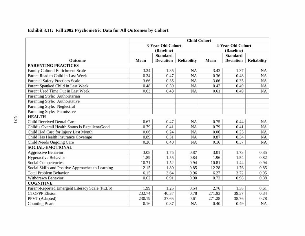
3-31
Exhibit 3.11: Fall 2002 Psychometric Data for All Outcomes by Cohort
Child Cohort
3-Year-Old Cohort
(Baseline) 4-Year-Old Cohort
(Baseline)
Outcome Mean Standard Deviation Reliability Mean
Standard Deviation Reliability
PARENTING PRACTICES Family Cultural Enrichment Scale 3.34 1.35 NA 3.43 1.37 NA Parent Read to Child in Last Week 0.34 0.47 NA 0.36 0.48 NA Parental Safety Practices Scale 3.66 0.35 NA 3.66 0.35 NA Parent Spanked Child in Last Week 0.48 0.50 NA 0.42 0.49 NA Parent Used Time Out in Last Week 0.63 0.48 NA 0.61 0.49 NA Parenting Style: Authoritarian Parenting Style: Authoritative Parenting Style: Neglectful Parenting Style: Permissive HEALTH Child Received Dental Care 0.67 0.47 NA 0.75 0.44 NA Child’s Overall Health Status Is Excellent/Good 0.79 0.41 NA 0.79 0.41 NA Child Had Care for Injury Last Month 0.06 0.24 NA 0.06 0.23 NA Child Has Health Insurance Coverage 0.89 0.31 NA 0.87 0.34 NA Child Needs Ongoing Care 0.20 0.40 NA 0.16 0.37 NA SOCIAL-EMOTIONAL Aggressive Behavior 3.08 1.75 0.87 3.01 1.73 0.85 Hyperactive Behavior 1.89 1.55 0.84 1.96 1.54 0.82 Social Competencies 10.71 1.52 0.94 10.81 1.44 0.94 Social Skills and Positive Approaches to Learning 12.15 1.80 0.85 12.28 1.76 0.85 Total Problem Behavior 6.15 3.64 0.96 6.27 3.72 0.95 Withdrawn Behavior 0.62 0.91 0.90 0.73 0.98 0.88 COGNITIVE Parent-Reported Emergent Literacy Scale (PELS) 1.99 1.25 0.54 2.76 1.38 0.61 CTOPPP Elision 232.74 40.37 0.78 271.93 39.37 0.84 PPVT (Adapted) 230.19 37.65 0.61 271.28 38.76 0.78 Counting Bears 0.16 0.37 NA 0.40 0.49 NA
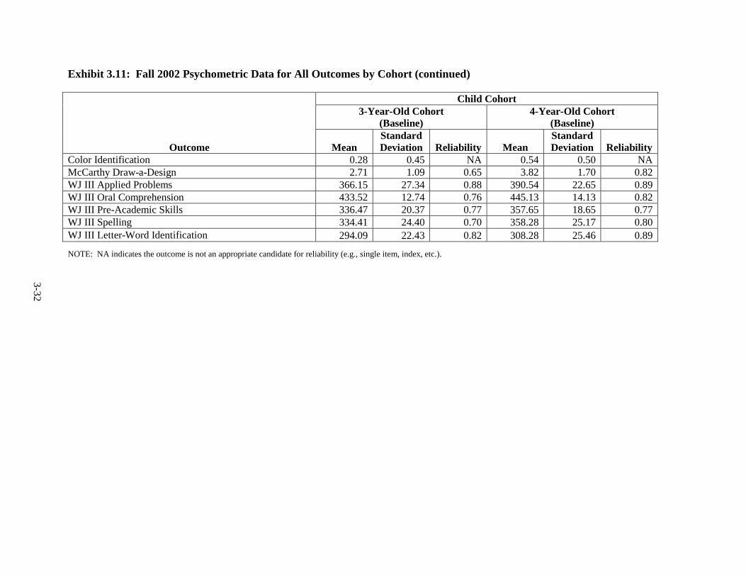
3-32
Exhibit 3.11: Fall 2002 Psychometric Data for All Outcomes by Cohort (continued) Child Cohort
3-Year-Old Cohort (Baseline)
4-Year-Old Cohort (Baseline)
Outcome Mean Standard Deviation Reliability Mean
Standard Deviation Reliability
Color Identification 0.28 0.45 NA 0.54 0.50 NA McCarthy Draw-a-Design 2.71 1.09 0.65 3.82 1.70 0.82 WJ III Applied Problems 366.15 27.34 0.88 390.54 22.65 0.89 WJ III Oral Comprehension 433.52 12.74 0.76 445.13 14.13 0.82 WJ III Pre-Academic Skills 336.47 20.37 0.77 357.65 18.65 0.77 WJ III Spelling 334.41 24.40 0.70 358.28 25.17 0.80 WJ III Letter-Word Identification 294.09 22.43 0.82 308.28 25.46 0.89
NOTE: NA indicates the outcome is not an appropriate candidate for reliability (e.g., single item, index, etc.).
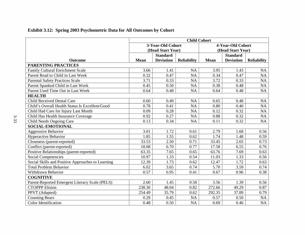
3-33
Exhibit 3.12: Spring 2003 Psychometric Data for All Outcomes by Cohort
Child Cohort
3-Year-Old Cohort (Head Start Year)
4-Year-Old Cohort (Head Start Year)
Outcome Mean Standard Deviation Reliability Mean
Standard Deviation Reliability
PARENTING PRACTICES Family Cultural Enrichment Scale 3.66 1.41 NA 3.95 1.43 NA Parent Read to Child in Last Week 0.32 0.47 NA 0.34 0.47 NA Parental Safety Practices Scale 3.71 0.33 NA 3.72 0.33 NA Parent Spanked Child in Last Week 0.45 0.50 NA 0.38 0.48 NA Parent Used Time Out in Last Week 0.64 0.48 NA 0.64 0.48 NA HEALTH Child Received Dental Care 0.60 0.49 NA 0.65 0.48 NA Child’s Overall Health Status Is Excellent/Good 0.78 0.41 NA 0.80 0.40 NA Child Had Care for Injury Last Month 0.09 0.28 NA 0.12 0.32 NA Child Has Health Insurance Coverage 0.92 0.27 NA 0.88 0.32 NA Child Needs Ongoing Care 0.13 0.34 NA 0.11 0.32 NA SOCIAL-EMOTIONAL Aggressive Behavior 3.01 1.72 0.61 2.79 1.68 0.56 Hyperactive Behavior 1.85 1.55 0.62 1.74 1.48 0.59 Closeness (parent-reported) 33.53 2.50 0.71 33.45 2.65 0.73 Conflict (parent-reported) 18.08 6.70 0.77 17.58 6.55 0.76 Positive Relationships (parent-reported) 63.35 7.65 0.65 63.76 7.69 0.63 Social Competencies 10.97 1.33 0.54 11.03 1.33 0.56 Social Skills and Positive Approaches to Learning 12.39 1.73 0.62 12.47 1.72 0.63 Total Problem Behavior 6.02 3.65 0.74 5.70 3.59 0.74 Withdrawn Behavior 0.57 0.95 0.41 0.67 0.96 0.38 COGNITIVE Parent-Reported Emergent Literacy Scale (PELS) 2.60 1.45 0.58 3.56 1.39 0.56 CTOPPP Elision 238.30 48.04 0.82 272.66 49.29 0.87 PPVT (Adapted) 254.49 35.79 0.62 292.35 37.89 0.79 Counting Bears 0.29 0.45 NA 0.57 0.50 NA Color Identification 0.48 0.50 NA 0.69 0.46 NA
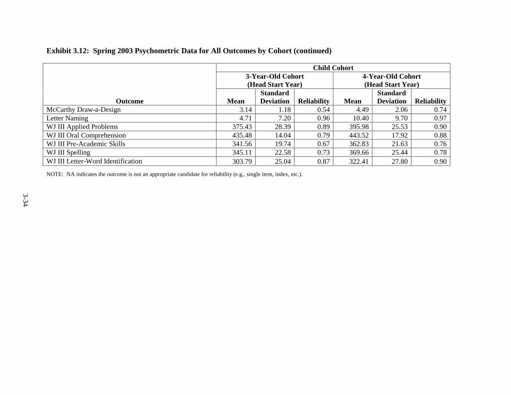
3-34
Exhibit 3.12: Spring 2003 Psychometric Data for All Outcomes by Cohort (continued)
Child Cohort
3-Year-Old Cohort (Head Start Year)
4-Year-Old Cohort (Head Start Year)
Outcome Mean Standard Deviation Reliability Mean
Standard Deviation Reliability
McCarthy Draw-a-Design 3.14 1.18 0.54 4.49 2.06 0.74 Letter Naming 4.71 7.20 0.96 10.40 9.70 0.97 WJ III Applied Problems 375.43 28.39 0.89 395.98 25.53 0.90 WJ III Oral Comprehension 435.48 14.04 0.79 443.52 17.92 0.88 WJ III Pre-Academic Skills 341.56 19.74 0.67 362.83 21.63 0.76 WJ III Spelling 345.11 22.58 0.73 369.66 25.44 0.78 WJ III Letter-Word Identification 303.79 25.04 0.87 322.41 27.80 0.90
NOTE: NA indicates the outcome is not an appropriate candidate for reliability (e.g., single item, index, etc.).
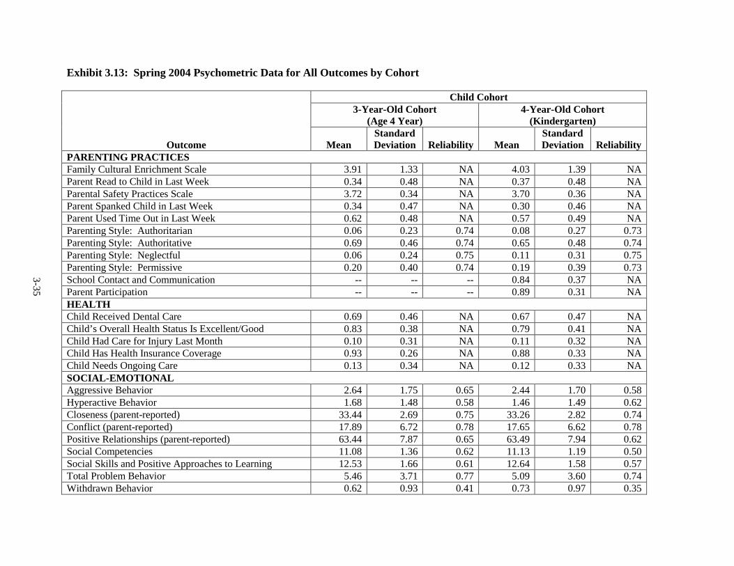
3-35
Exhibit 3.13: Spring 2004 Psychometric Data for All Outcomes by Cohort Child Cohort
3-Year-Old Cohort (Age 4 Year)
4-Year-Old Cohort (Kindergarten)
Outcome Mean Standard Deviation Reliability Mean
Standard Deviation Reliability
PARENTING PRACTICES Family Cultural Enrichment Scale 3.91 1.33 NA 4.03 1.39 NA Parent Read to Child in Last Week 0.34 0.48 NA 0.37 0.48 NA Parental Safety Practices Scale 3.72 0.34 NA 3.70 0.36 NA Parent Spanked Child in Last Week 0.34 0.47 NA 0.30 0.46 NA Parent Used Time Out in Last Week 0.62 0.48 NA 0.57 0.49 NA Parenting Style: Authoritarian 0.06 0.23 0.74 0.08 0.27 0.73 Parenting Style: Authoritative 0.69 0.46 0.74 0.65 0.48 0.74 Parenting Style: Neglectful 0.06 0.24 0.75 0.11 0.31 0.75 Parenting Style: Permissive 0.20 0.40 0.74 0.19 0.39 0.73 School Contact and Communication -- -- -- 0.84 0.37 NA Parent Participation -- -- -- 0.89 0.31 NA HEALTH Child Received Dental Care 0.69 0.46 NA 0.67 0.47 NA Child’s Overall Health Status Is Excellent/Good 0.83 0.38 NA 0.79 0.41 NA Child Had Care for Injury Last Month 0.10 0.31 NA 0.11 0.32 NA Child Has Health Insurance Coverage 0.93 0.26 NA 0.88 0.33 NA Child Needs Ongoing Care 0.13 0.34 NA 0.12 0.33 NA SOCIAL-EMOTIONAL Aggressive Behavior 2.64 1.75 0.65 2.44 1.70 0.58 Hyperactive Behavior 1.68 1.48 0.58 1.46 1.49 0.62 Closeness (parent-reported) 33.44 2.69 0.75 33.26 2.82 0.74 Conflict (parent-reported) 17.89 6.72 0.78 17.65 6.62 0.78 Positive Relationships (parent-reported) 63.44 7.87 0.65 63.49 7.94 0.62 Social Competencies 11.08 1.36 0.62 11.13 1.19 0.50 Social Skills and Positive Approaches to Learning 12.53 1.66 0.61 12.64 1.58 0.57 Total Problem Behavior 5.46 3.71 0.77 5.09 3.60 0.74 Withdrawn Behavior 0.62 0.93 0.41 0.73 0.97 0.35
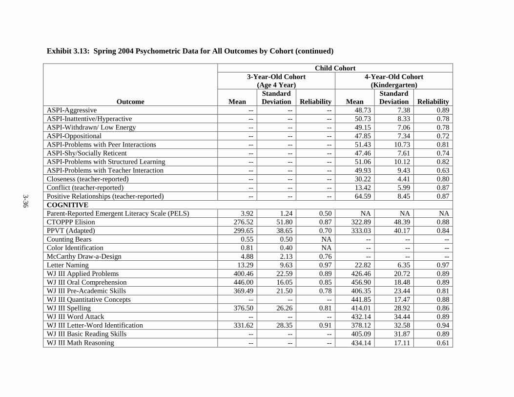
3-36
Exhibit 3.13: Spring 2004 Psychometric Data for All Outcomes by Cohort (continued) Child Cohort 3-Year-Old Cohort
(Age 4 Year) 4-Year-Old Cohort
(Kindergarten)
Outcome Mean Standard Deviation Reliability Mean
Standard Deviation Reliability
ASPI-Aggressive -- -- -- 48.73 7.38 0.89 ASPI-Inattentive/Hyperactive -- -- -- 50.73 8.33 0.78 ASPI-Withdrawn/ Low Energy -- -- -- 49.15 7.06 0.78 ASPI-Oppositional -- -- -- 47.85 7.34 0.72 ASPI-Problems with Peer Interactions -- -- -- 51.43 10.73 0.81 ASPI-Shy/Socially Reticent -- -- -- 47.46 7.61 0.74 ASPI-Problems with Structured Learning -- -- -- 51.06 10.12 0.82 ASPI-Problems with Teacher Interaction -- -- -- 49.93 9.43 0.63 Closeness (teacher-reported) -- -- -- 30.22 4.41 0.80 Conflict (teacher-reported) -- -- -- 13.42 5.99 0.87 Positive Relationships (teacher-reported) -- -- -- 64.59 8.45 0.87 COGNITIVE Parent-Reported Emergent Literacy Scale (PELS) 3.92 1.24 0.50 NA NA NA CTOPPP Elision 276.52 51.80 0.87 322.89 48.39 0.88 PPVT (Adapted) 299.65 38.65 0.70 333.03 40.17 0.84 Counting Bears 0.55 0.50 NA -- -- -- Color Identification 0.81 0.40 NA -- -- -- McCarthy Draw-a-Design 4.88 2.13 0.76 -- -- -- Letter Naming 13.29 9.63 0.97 22.82 6.35 0.97 WJ III Applied Problems 400.46 22.59 0.89 426.46 20.72 0.89 WJ III Oral Comprehension 446.00 16.05 0.85 456.90 18.48 0.89 WJ III Pre-Academic Skills 369.49 21.50 0.78 406.35 23.44 0.81 WJ III Quantitative Concepts -- -- -- 441.85 17.47 0.88 WJ III Spelling 376.50 26.26 0.81 414.01 28.92 0.86 WJ III Word Attack -- -- -- 432.14 34.44 0.89 WJ III Letter-Word Identification 331.62 28.35 0.91 378.12 32.58 0.94 WJ III Basic Reading Skills -- -- -- 405.09 31.87 0.89 WJ III Math Reasoning -- -- -- 434.14 17.11 0.61
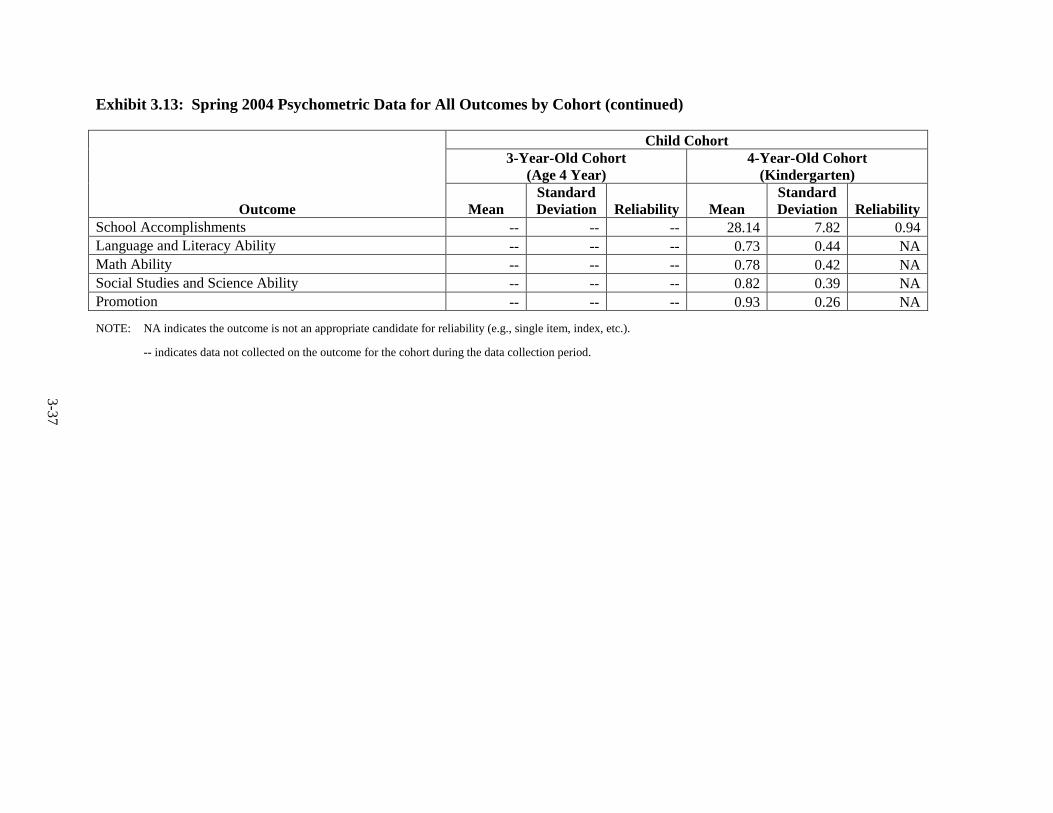
3-37
Exhibit 3.13: Spring 2004 Psychometric Data for All Outcomes by Cohort (continued) Child Cohort
3-Year-Old Cohort (Age 4 Year)
4-Year-Old Cohort (Kindergarten)
Outcome Mean Standard Deviation Reliability Mean
Standard Deviation Reliability
School Accomplishments -- -- -- 28.14 7.82 0.94 Language and Literacy Ability -- -- -- 0.73 0.44 NA Math Ability -- -- -- 0.78 0.42 NA Social Studies and Science Ability -- -- -- 0.82 0.39 NA Promotion -- -- -- 0.93 0.26 NA
NOTE: NA indicates the outcome is not an appropriate candidate for reliability (e.g., single item, index, etc.).
-- indicates data not collected on the outcome for the cohort during the data collection period.
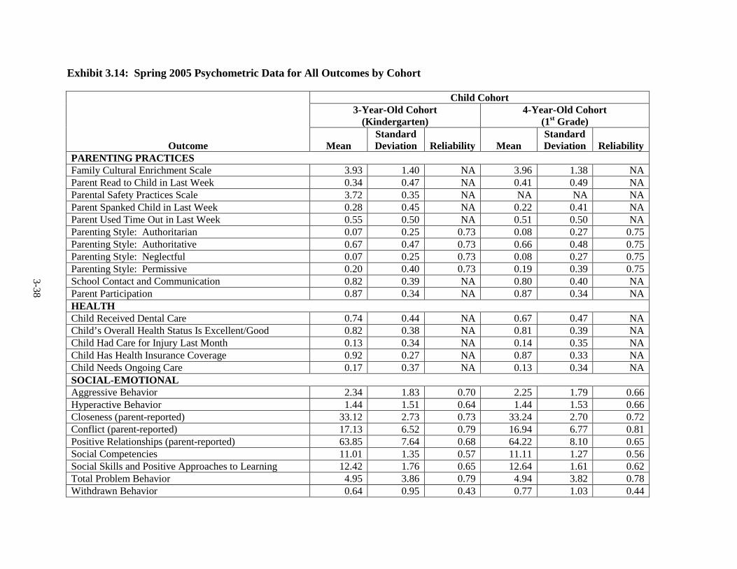
3-38
Exhibit 3.14: Spring 2005 Psychometric Data for All Outcomes by Cohort
Child Cohort
3-Year-Old Cohort
(Kindergarten) 4-Year-Old Cohort
(1st Grade)
Outcome Mean Standard Deviation Reliability Mean
Standard Deviation Reliability
PARENTING PRACTICES Family Cultural Enrichment Scale 3.93 1.40 NA 3.96 1.38 NA Parent Read to Child in Last Week 0.34 0.47 NA 0.41 0.49 NA Parental Safety Practices Scale 3.72 0.35 NA NA NA NA Parent Spanked Child in Last Week 0.28 0.45 NA 0.22 0.41 NA Parent Used Time Out in Last Week 0.55 0.50 NA 0.51 0.50 NA Parenting Style: Authoritarian 0.07 0.25 0.73 0.08 0.27 0.75 Parenting Style: Authoritative 0.67 0.47 0.73 0.66 0.48 0.75 Parenting Style: Neglectful 0.07 0.25 0.73 0.08 0.27 0.75 Parenting Style: Permissive 0.20 0.40 0.73 0.19 0.39 0.75 School Contact and Communication 0.82 0.39 NA 0.80 0.40 NA Parent Participation 0.87 0.34 NA 0.87 0.34 NA HEALTH Child Received Dental Care 0.74 0.44 NA 0.67 0.47 NA Child’s Overall Health Status Is Excellent/Good 0.82 0.38 NA 0.81 0.39 NA Child Had Care for Injury Last Month 0.13 0.34 NA 0.14 0.35 NA Child Has Health Insurance Coverage 0.92 0.27 NA 0.87 0.33 NA Child Needs Ongoing Care 0.17 0.37 NA 0.13 0.34 NA SOCIAL-EMOTIONAL Aggressive Behavior 2.34 1.83 0.70 2.25 1.79 0.66 Hyperactive Behavior 1.44 1.51 0.64 1.44 1.53 0.66 Closeness (parent-reported) 33.12 2.73 0.73 33.24 2.70 0.72 Conflict (parent-reported) 17.13 6.52 0.79 16.94 6.77 0.81 Positive Relationships (parent-reported) 63.85 7.64 0.68 64.22 8.10 0.65 Social Competencies 11.01 1.35 0.57 11.11 1.27 0.56 Social Skills and Positive Approaches to Learning 12.42 1.76 0.65 12.64 1.61 0.62 Total Problem Behavior 4.95 3.86 0.79 4.94 3.82 0.78 Withdrawn Behavior 0.64 0.95 0.43 0.77 1.03 0.44
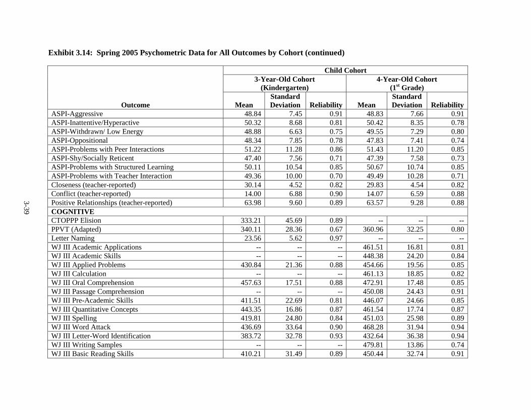
3-39
Exhibit 3.14: Spring 2005 Psychometric Data for All Outcomes by Cohort (continued)
Child Cohort
3-Year-Old Cohort
(Kindergarten) 4-Year-Old Cohort
(1st Grade)
Outcome Mean Standard Deviation Reliability Mean
Standard Deviation Reliability
ASPI-Aggressive 48.84 7.45 0.91 48.83 7.66 0.91 ASPI-Inattentive/Hyperactive 50.32 8.68 0.81 50.42 8.35 0.78 ASPI-Withdrawn/ Low Energy 48.88 6.63 0.75 49.55 7.29 0.80 ASPI-Oppositional 48.34 7.85 0.78 47.83 7.41 0.74 ASPI-Problems with Peer Interactions 51.22 11.28 0.86 51.43 11.20 0.85 ASPI-Shy/Socially Reticent 47.40 7.56 0.71 47.39 7.58 0.73 ASPI-Problems with Structured Learning 50.11 10.54 0.85 50.67 10.74 0.85 ASPI-Problems with Teacher Interaction 49.36 10.00 0.70 49.49 10.28 0.71 Closeness (teacher-reported) 30.14 4.52 0.82 29.83 4.54 0.82 Conflict (teacher-reported) 14.00 6.88 0.90 14.07 6.59 0.88 Positive Relationships (teacher-reported) 63.98 9.60 0.89 63.57 9.28 0.88 COGNITIVE CTOPPP Elision 333.21 45.69 0.89 -- -- -- PPVT (Adapted) 340.11 28.36 0.67 360.96 32.25 0.80 Letter Naming 23.56 5.62 0.97 -- -- -- WJ III Academic Applications -- -- -- 461.51 16.81 0.81 WJ III Academic Skills -- -- -- 448.38 24.20 0.84 WJ III Applied Problems 430.84 21.36 0.88 454.66 19.56 0.85 WJ III Calculation -- -- -- 461.13 18.85 0.82 WJ III Oral Comprehension 457.63 17.51 0.88 472.91 17.48 0.85 WJ III Passage Comprehension -- -- -- 450.08 24.43 0.91 WJ III Pre-Academic Skills 411.51 22.69 0.81 446.07 24.66 0.85 WJ III Quantitative Concepts 443.35 16.86 0.87 461.54 17.74 0.87 WJ III Spelling 419.81 24.80 0.84 451.03 25.98 0.89 WJ III Word Attack 436.69 33.64 0.90 468.28 31.94 0.94 WJ III Letter-Word Identification 383.72 32.78 0.93 432.64 36.38 0.94 WJ III Writing Samples -- -- -- 479.81 13.86 0.74 WJ III Basic Reading Skills 410.21 31.49 0.89 450.44 32.74 0.91
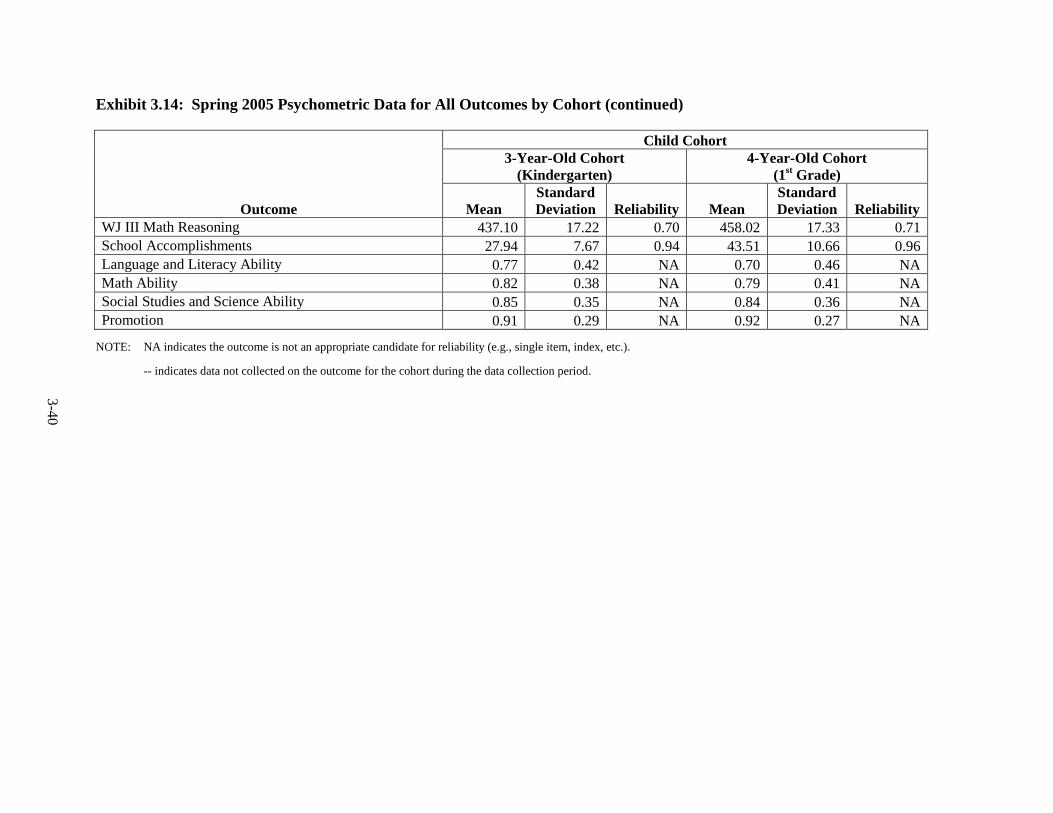
3-40
Exhibit 3.14: Spring 2005 Psychometric Data for All Outcomes by Cohort (continued) Child Cohort
3-Year-Old Cohort (Kindergarten)
4-Year-Old Cohort (1st Grade)
Outcome Mean Standard Deviation Reliability Mean
Standard Deviation Reliability
WJ III Math Reasoning 437.10 17.22 0.70 458.02 17.33 0.71 School Accomplishments 27.94 7.67 0.94 43.51 10.66 0.96 Language and Literacy Ability 0.77 0.42 NA 0.70 0.46 NA Math Ability 0.82 0.38 NA 0.79 0.41 NA Social Studies and Science Ability 0.85 0.35 NA 0.84 0.36 NA Promotion 0.91 0.29 NA 0.92 0.27 NA
NOTE: NA indicates the outcome is not an appropriate candidate for reliability (e.g., single item, index, etc.).
-- indicates data not collected on the outcome for the cohort during the data collection period.
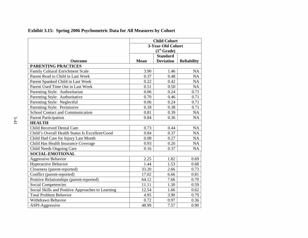
3-41
Exhibit 3.15: Spring 2006 Psychometric Data for All Measures by Cohort
Child Cohort
3-Year-Old Cohort
(1st Grade)
Outcome Mean StandardDeviation Reliability
PARENTING PRACTICES Family Cultural Enrichment Scale 3.90 1.46 NA Parent Read to Child in Last Week 0.37 0.48 NA Parent Spanked Child in Last Week 0.22 0.42 NA Parent Used Time Out in Last Week 0.51 0.50 NA Parenting Style: Authoritarian 0.06 0.24 0.71 Parenting Style: Authoritative 0.70 0.46 0.71 Parenting Style: Neglectful 0.06 0.24 0.71 Parenting Style: Permissive 0.18 0.38 0.71 School Contact and Communication 0.81 0.39 NA Parent Participation 0.84 0.36 NA HEALTH Child Received Dental Care 0.73 0.44 NA Child’s Overall Health Status Is Excellent/Good 0.84 0.37 NA Child Had Care for Injury Last Month 0.08 0.27 NA Child Has Health Insurance Coverage 0.93 0.26 NA Child Needs Ongoing Care 0.16 0.37 NA SOCIAL-EMOTIONAL Aggressive Behavior 2.25 1.82 0.69 Hyperactive Behavior 1.44 1.53 0.68 Closeness (parent-reported) 33.20 2.66 0.73 Conflict (parent-reported) 17.02 6.66 0.81 Positive Relationships (parent-reported) 64.12 7.66 0.70 Social Competencies 11.11 1.30 0.59 Social Skills and Positive Approaches to Learning 12.54 1.66 0.62 Total Problem Behavior 4.95 3.90 0.79 Withdrawn Behavior 0.72 0.97 0.36 ASPI-Aggressive 48.99 7.57 0.90
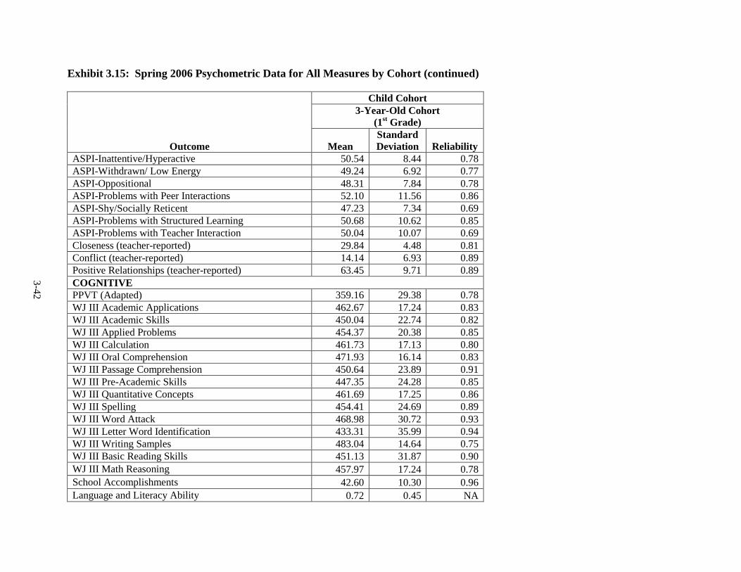
3-42
Exhibit 3.15: Spring 2006 Psychometric Data for All Measures by Cohort (continued) Child Cohort 3-Year-Old Cohort
(1st Grade)
Outcome Mean StandardDeviation Reliability
ASPI-Inattentive/Hyperactive 50.54 8.44 0.78 ASPI-Withdrawn/ Low Energy 49.24 6.92 0.77 ASPI-Oppositional 48.31 7.84 0.78 ASPI-Problems with Peer Interactions 52.10 11.56 0.86 ASPI-Shy/Socially Reticent 47.23 7.34 0.69 ASPI-Problems with Structured Learning 50.68 10.62 0.85 ASPI-Problems with Teacher Interaction 50.04 10.07 0.69 Closeness (teacher-reported) 29.84 4.48 0.81 Conflict (teacher-reported) 14.14 6.93 0.89 Positive Relationships (teacher-reported) 63.45 9.71 0.89 COGNITIVE PPVT (Adapted) 359.16 29.38 0.78 WJ III Academic Applications 462.67 17.24 0.83 WJ III Academic Skills 450.04 22.74 0.82 WJ III Applied Problems 454.37 20.38 0.85 WJ III Calculation 461.73 17.13 0.80 WJ III Oral Comprehension 471.93 16.14 0.83 WJ III Passage Comprehension 450.64 23.89 0.91 WJ III Pre-Academic Skills 447.35 24.28 0.85 WJ III Quantitative Concepts 461.69 17.25 0.86 WJ III Spelling 454.41 24.69 0.89 WJ III Word Attack 468.98 30.72 0.93 WJ III Letter Word Identification 433.31 35.99 0.94 WJ III Writing Samples 483.04 14.64 0.75 WJ III Basic Reading Skills 451.13 31.87 0.90 WJ III Math Reasoning 457.97 17.24 0.78 School Accomplishments 42.60 10.30 0.96 Language and Literacy Ability 0.72 0.45 NA
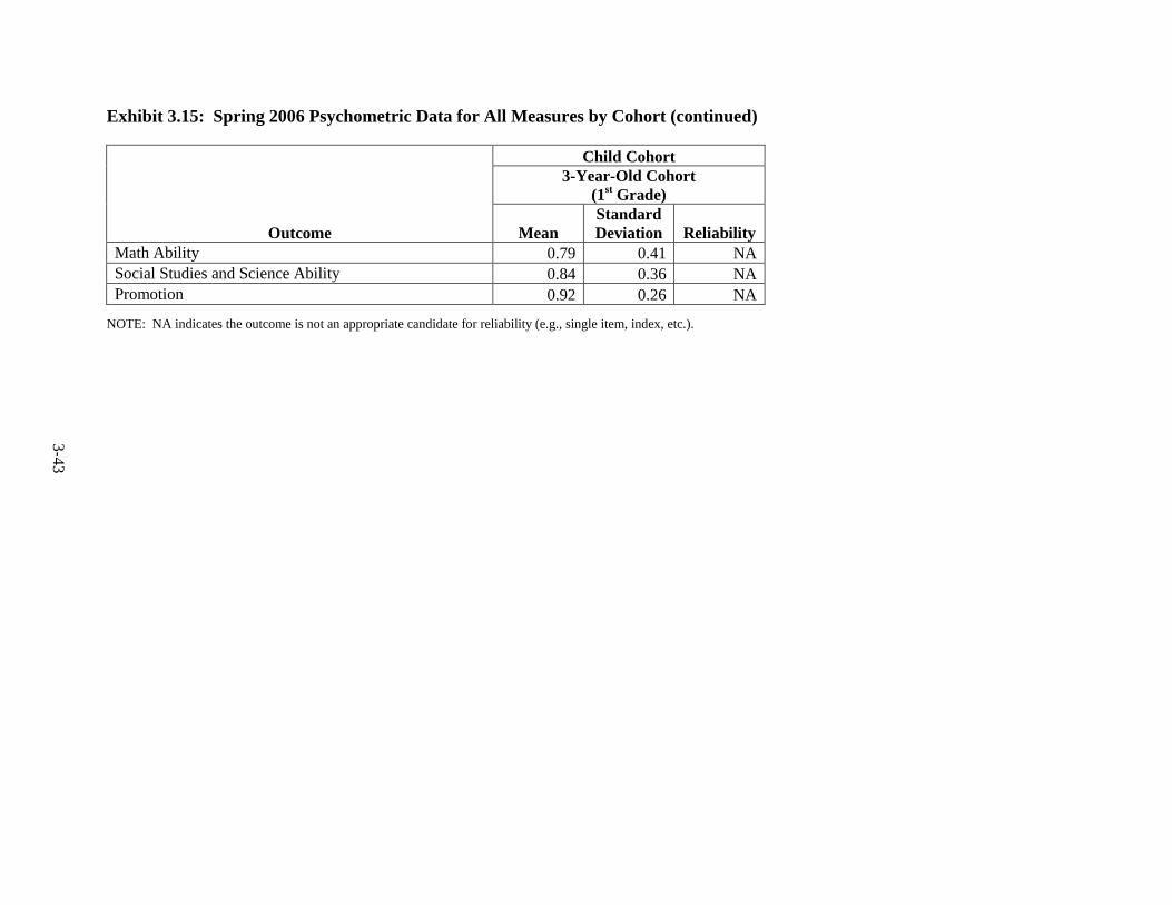
3-43
Exhibit 3.15: Spring 2006 Psychometric Data for All Measures by Cohort (continued) Child Cohort
3-Year-Old Cohort (1st Grade)
Outcome Mean StandardDeviation Reliability
Math Ability 0.79 0.41 NA Social Studies and Science Ability 0.84 0.36 NA Promotion 0.92 0.26 NA
NOTE: NA indicates the outcome is not an appropriate candidate for reliability (e.g., single item, index, etc.).
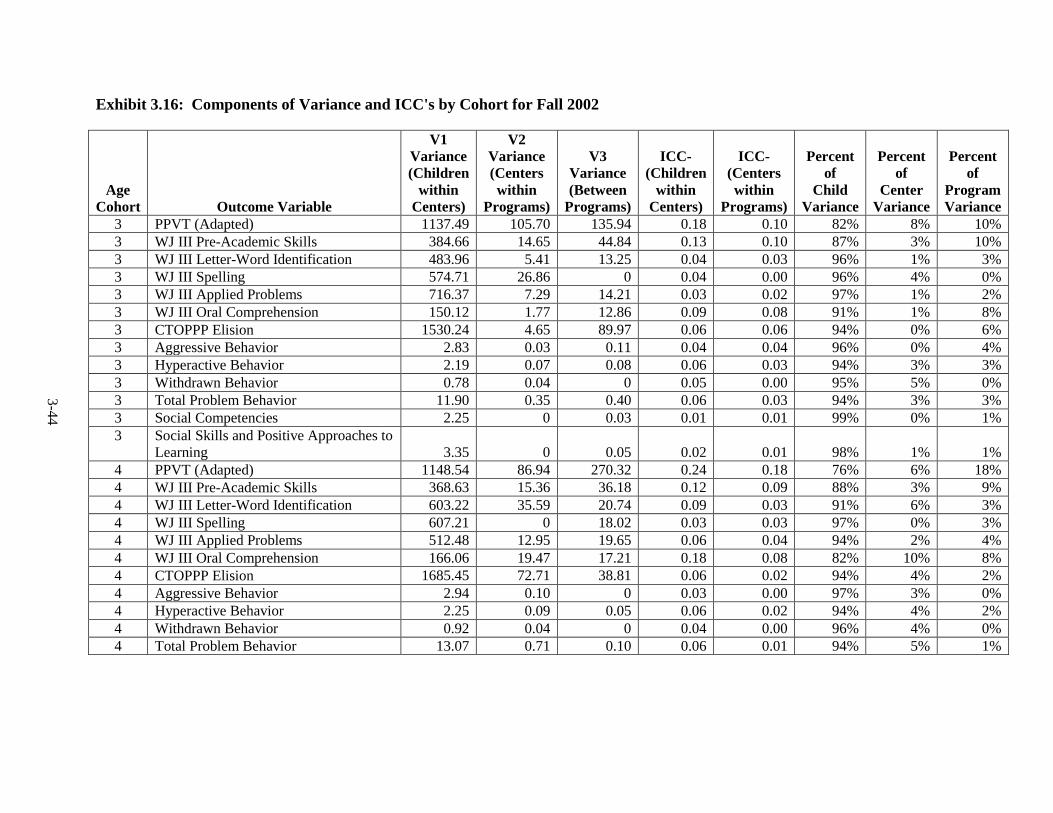
3-44
Exhibit 3.16: Components of Variance and ICC's by Cohort for Fall 2002
Age Cohort Outcome Variable
V1 Variance (Children
within Centers)
V2 Variance (Centers within
Programs)
V3 Variance (Between
Programs)
ICC- (Children
within Centers)
ICC-(Centers within
Programs)
Percent of
Child Variance
Percent of
Center Variance
Percent of
Program Variance
3 PPVT (Adapted) 1137.49 105.70 135.94 0.18 0.10 82% 8% 10% 3 WJ III Pre-Academic Skills 384.66 14.65 44.84 0.13 0.10 87% 3% 10% 3 WJ III Letter-Word Identification 483.96 5.41 13.25 0.04 0.03 96% 1% 3% 3 WJ III Spelling 574.71 26.86 0 0.04 0.00 96% 4% 0% 3 WJ III Applied Problems 716.37 7.29 14.21 0.03 0.02 97% 1% 2% 3 WJ III Oral Comprehension 150.12 1.77 12.86 0.09 0.08 91% 1% 8% 3 CTOPPP Elision 1530.24 4.65 89.97 0.06 0.06 94% 0% 6% 3 Aggressive Behavior 2.83 0.03 0.11 0.04 0.04 96% 0% 4% 3 Hyperactive Behavior 2.19 0.07 0.08 0.06 0.03 94% 3% 3% 3 Withdrawn Behavior 0.78 0.04 0 0.05 0.00 95% 5% 0% 3 Total Problem Behavior 11.90 0.35 0.40 0.06 0.03 94% 3% 3% 3 Social Competencies 2.25 0 0.03 0.01 0.01 99% 0% 1% 3 Social Skills and Positive Approaches to
Learning 3.35 0 0.05 0.02 0.01 98% 1% 1% 4 PPVT (Adapted) 1148.54 86.94 270.32 0.24 0.18 76% 6% 18% 4 WJ III Pre-Academic Skills 368.63 15.36 36.18 0.12 0.09 88% 3% 9% 4 WJ III Letter-Word Identification 603.22 35.59 20.74 0.09 0.03 91% 6% 3% 4 WJ III Spelling 607.21 0 18.02 0.03 0.03 97% 0% 3% 4 WJ III Applied Problems 512.48 12.95 19.65 0.06 0.04 94% 2% 4% 4 WJ III Oral Comprehension 166.06 19.47 17.21 0.18 0.08 82% 10% 8% 4 CTOPPP Elision 1685.45 72.71 38.81 0.06 0.02 94% 4% 2% 4 Aggressive Behavior 2.94 0.10 0 0.03 0.00 97% 3% 0% 4 Hyperactive Behavior 2.25 0.09 0.05 0.06 0.02 94% 4% 2% 4 Withdrawn Behavior 0.92 0.04 0 0.04 0.00 96% 4% 0% 4 Total Problem Behavior 13.07 0.71 0.10 0.06 0.01 94% 5% 1%
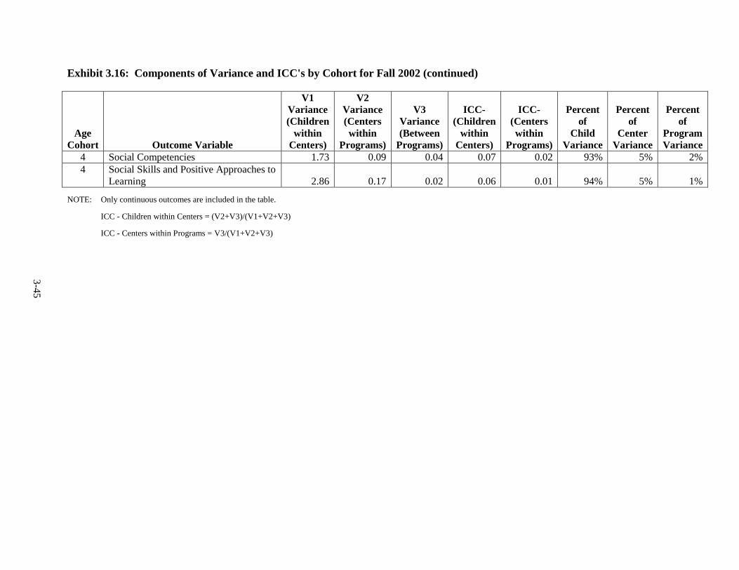
3-45
Exhibit 3.16: Components of Variance and ICC's by Cohort for Fall 2002 (continued)
Age Cohort Outcome Variable
V1 Variance (Children
within Centers)
V2 Variance (Centers within
Programs)
V3 Variance (Between
Programs)
ICC- (Children
within Centers)
ICC-(Centers within
Programs)
Percent of
Child Variance
Percent of
Center Variance
Percent of
Program Variance
4 Social Competencies 1.73 0.09 0.04 0.07 0.02 93% 5% 2% 4 Social Skills and Positive Approaches to
Learning 2.86 0.17 0.02 0.06 0.01 94% 5% 1%
NOTE: Only continuous outcomes are included in the table.
ICC - Children within Centers = (V2+V3)/(V1+V2+V3)
ICC - Centers within Programs = V3/(V1+V2+V3)
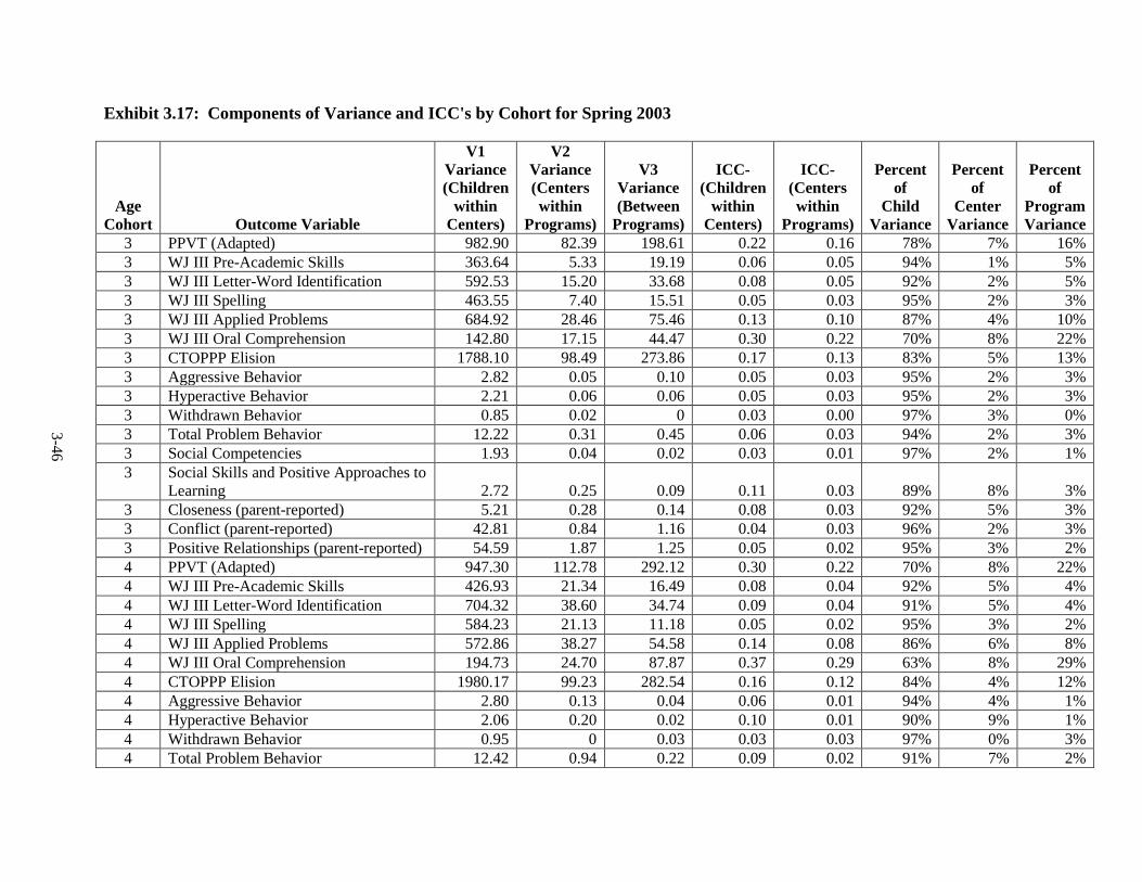
3-46
Exhibit 3.17: Components of Variance and ICC's by Cohort for Spring 2003
Age Cohort Outcome Variable
V1 Variance (Children
within Centers)
V2 Variance (Centers within
Programs)
V3 Variance (Between
Programs)
ICC- (Children
within Centers)
ICC-(Centers within
Programs)
Percent of
Child Variance
Percent of
Center Variance
Percent of
Program Variance
3 PPVT (Adapted) 982.90 82.39 198.61 0.22 0.16 78% 7% 16% 3 WJ III Pre-Academic Skills 363.64 5.33 19.19 0.06 0.05 94% 1% 5% 3 WJ III Letter-Word Identification 592.53 15.20 33.68 0.08 0.05 92% 2% 5% 3 WJ III Spelling 463.55 7.40 15.51 0.05 0.03 95% 2% 3% 3 WJ III Applied Problems 684.92 28.46 75.46 0.13 0.10 87% 4% 10% 3 WJ III Oral Comprehension 142.80 17.15 44.47 0.30 0.22 70% 8% 22% 3 CTOPPP Elision 1788.10 98.49 273.86 0.17 0.13 83% 5% 13% 3 Aggressive Behavior 2.82 0.05 0.10 0.05 0.03 95% 2% 3% 3 Hyperactive Behavior 2.21 0.06 0.06 0.05 0.03 95% 2% 3% 3 Withdrawn Behavior 0.85 0.02 0 0.03 0.00 97% 3% 0% 3 Total Problem Behavior 12.22 0.31 0.45 0.06 0.03 94% 2% 3% 3 Social Competencies 1.93 0.04 0.02 0.03 0.01 97% 2% 1% 3 Social Skills and Positive Approaches to
Learning 2.72 0.25 0.09 0.11 0.03 89% 8% 3% 3 Closeness (parent-reported) 5.21 0.28 0.14 0.08 0.03 92% 5% 3% 3 Conflict (parent-reported) 42.81 0.84 1.16 0.04 0.03 96% 2% 3% 3 Positive Relationships (parent-reported) 54.59 1.87 1.25 0.05 0.02 95% 3% 2% 4 PPVT (Adapted) 947.30 112.78 292.12 0.30 0.22 70% 8% 22% 4 WJ III Pre-Academic Skills 426.93 21.34 16.49 0.08 0.04 92% 5% 4% 4 WJ III Letter-Word Identification 704.32 38.60 34.74 0.09 0.04 91% 5% 4% 4 WJ III Spelling 584.23 21.13 11.18 0.05 0.02 95% 3% 2% 4 WJ III Applied Problems 572.86 38.27 54.58 0.14 0.08 86% 6% 8% 4 WJ III Oral Comprehension 194.73 24.70 87.87 0.37 0.29 63% 8% 29% 4 CTOPPP Elision 1980.17 99.23 282.54 0.16 0.12 84% 4% 12% 4 Aggressive Behavior 2.80 0.13 0.04 0.06 0.01 94% 4% 1% 4 Hyperactive Behavior 2.06 0.20 0.02 0.10 0.01 90% 9% 1% 4 Withdrawn Behavior 0.95 0 0.03 0.03 0.03 97% 0% 3% 4 Total Problem Behavior 12.42 0.94 0.22 0.09 0.02 91% 7% 2%
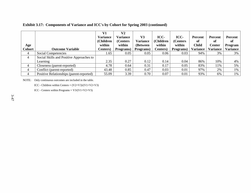
3-47
Exhibit 3.17: Components of Variance and ICC's by Cohort for Spring 2003 (continued)
Age Cohort Outcome Variable
V1 Variance (Children
within Centers)
V2 Variance (Centers within
Programs)
V3 Variance (Between
Programs)
ICC- (Children
within Centers)
ICC-(Centers within
Programs)
Percent of
Child Variance
Percent of
Center Variance
Percent of
Program Variance
4 Social Competencies 1.65 0.05 0.05 0.06 0.03 94% 3% 3% 4 Social Skills and Positive Approaches to
Learning 2.35 0.27 0.12 0.14 0.04 86% 10% 4% 4 Closeness (parent-reported) 4.78 0.64 0.31 0.17 0.05 83% 11% 5% 4 Conflict (parent-reported) 43.48 0.85 0.47 0.03 0.01 97% 2% 1% 4 Positive Relationships (parent-reported) 55.09 3.39 0.70 0.07 0.01 93% 6% 1%
NOTE: Only continuous outcomes are included in the table.
ICC - Children within Centers = (V2+V3)/(V1+V2+V3)
ICC - Centers within Programs = V3/(V1+V2+V3)
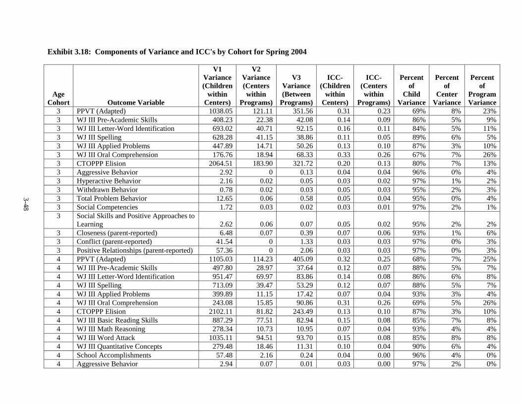
3-48
Exhibit 3.18: Components of Variance and ICC's by Cohort for Spring 2004
Age Cohort Outcome Variable
V1 Variance (Children
within Centers)
V2 Variance (Centers within
Programs)
V3 Variance (Between
Programs)
ICC- (Children
within Centers)
ICC-(Centers within
Programs)
Percent of
Child Variance
Percent of
Center Variance
Percent of
Program Variance
3 PPVT (Adapted) 1038.05 121.11 351.56 0.31 0.23 69% 8% 23% 3 WJ III Pre-Academic Skills 408.23 22.38 42.08 0.14 0.09 86% 5% 9% 3 WJ III Letter-Word Identification 693.02 40.71 92.15 0.16 0.11 84% 5% 11% 3 WJ III Spelling 628.28 41.15 38.86 0.11 0.05 89% 6% 5% 3 WJ III Applied Problems 447.89 14.71 50.26 0.13 0.10 87% 3% 10% 3 WJ III Oral Comprehension 176.76 18.94 68.33 0.33 0.26 67% 7% 26% 3 CTOPPP Elision 2064.51 183.90 321.72 0.20 0.13 80% 7% 13% 3 Aggressive Behavior 2.92 0 0.13 0.04 0.04 96% 0% 4% 3 Hyperactive Behavior 2.16 0.02 0.05 0.03 0.02 97% 1% 2% 3 Withdrawn Behavior 0.78 0.02 0.03 0.05 0.03 95% 2% 3% 3 Total Problem Behavior 12.65 0.06 0.58 0.05 0.04 95% 0% 4% 3 Social Competencies 1.72 0.03 0.02 0.03 0.01 97% 2% 1% 3 Social Skills and Positive Approaches to
Learning 2.62 0.06 0.07 0.05 0.02 95% 2% 2% 3 Closeness (parent-reported) 6.48 0.07 0.39 0.07 0.06 93% 1% 6% 3 Conflict (parent-reported) 41.54 0 1.33 0.03 0.03 97% 0% 3% 3 Positive Relationships (parent-reported) 57.36 0 2.06 0.03 0.03 97% 0% 3% 4 PPVT (Adapted) 1105.03 114.23 405.09 0.32 0.25 68% 7% 25% 4 WJ III Pre-Academic Skills 497.80 28.97 37.64 0.12 0.07 88% 5% 7% 4 WJ III Letter-Word Identification 951.47 69.97 83.86 0.14 0.08 86% 6% 8% 4 WJ III Spelling 713.09 39.47 53.29 0.12 0.07 88% 5% 7% 4 WJ III Applied Problems 399.89 11.15 17.42 0.07 0.04 93% 3% 4% 4 WJ III Oral Comprehension 243.08 15.85 90.86 0.31 0.26 69% 5% 26% 4 CTOPPP Elision 2102.11 81.82 243.49 0.13 0.10 87% 3% 10% 4 WJ III Basic Reading Skills 887.29 77.51 82.94 0.15 0.08 85% 7% 8% 4 WJ III Math Reasoning 278.34 10.73 10.95 0.07 0.04 93% 4% 4% 4 WJ III Word Attack 1035.11 94.51 93.70 0.15 0.08 85% 8% 8% 4 WJ III Quantitative Concepts 279.48 18.46 11.31 0.10 0.04 90% 6% 4% 4 School Accomplishments 57.48 2.16 0.24 0.04 0.00 96% 4% 0% 4 Aggressive Behavior 2.94 0.07 0.01 0.03 0.00 97% 2% 0%
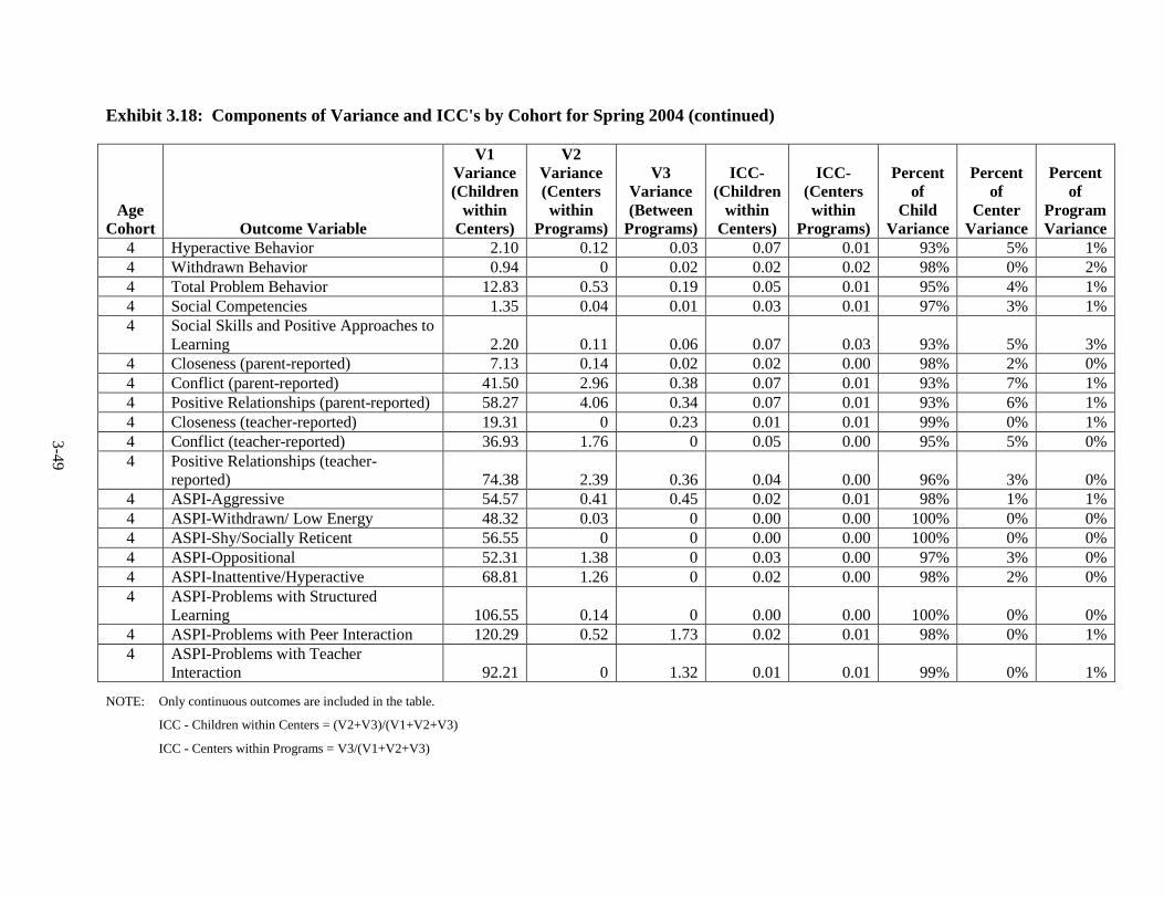
3-49
Exhibit 3.18: Components of Variance and ICC's by Cohort for Spring 2004 (continued)
Age Cohort Outcome Variable
V1 Variance (Children
within Centers)
V2 Variance (Centers within
Programs)
V3 Variance (Between
Programs)
ICC- (Children
within Centers)
ICC-(Centers within
Programs)
Percent of
Child Variance
Percent of
Center Variance
Percent of
Program Variance
4 Hyperactive Behavior 2.10 0.12 0.03 0.07 0.01 93% 5% 1% 4 Withdrawn Behavior 0.94 0 0.02 0.02 0.02 98% 0% 2% 4 Total Problem Behavior 12.83 0.53 0.19 0.05 0.01 95% 4% 1% 4 Social Competencies 1.35 0.04 0.01 0.03 0.01 97% 3% 1% 4 Social Skills and Positive Approaches to
Learning 2.20 0.11 0.06 0.07 0.03 93% 5% 3% 4 Closeness (parent-reported) 7.13 0.14 0.02 0.02 0.00 98% 2% 0% 4 Conflict (parent-reported) 41.50 2.96 0.38 0.07 0.01 93% 7% 1% 4 Positive Relationships (parent-reported) 58.27 4.06 0.34 0.07 0.01 93% 6% 1% 4 Closeness (teacher-reported) 19.31 0 0.23 0.01 0.01 99% 0% 1% 4 Conflict (teacher-reported) 36.93 1.76 0 0.05 0.00 95% 5% 0% 4 Positive Relationships (teacher-
reported) 74.38 2.39 0.36 0.04 0.00 96% 3% 0% 4 ASPI-Aggressive 54.57 0.41 0.45 0.02 0.01 98% 1% 1% 4 ASPI-Withdrawn/ Low Energy 48.32 0.03 0 0.00 0.00 100% 0% 0% 4 ASPI-Shy/Socially Reticent 56.55 0 0 0.00 0.00 100% 0% 0% 4 ASPI-Oppositional 52.31 1.38 0 0.03 0.00 97% 3% 0% 4 ASPI-Inattentive/Hyperactive 68.81 1.26 0 0.02 0.00 98% 2% 0% 4 ASPI-Problems with Structured
Learning 106.55 0.14 0 0.00 0.00 100% 0% 0% 4 ASPI-Problems with Peer Interaction 120.29 0.52 1.73 0.02 0.01 98% 0% 1% 4 ASPI-Problems with Teacher
Interaction 92.21 0 1.32 0.01 0.01 99% 0% 1%
NOTE: Only continuous outcomes are included in the table.
ICC - Children within Centers = (V2+V3)/(V1+V2+V3)
ICC - Centers within Programs = V3/(V1+V2+V3)
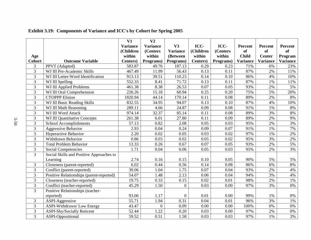
3-50
Exhibit 3.19: Components of Variance and ICC's by Cohort for Spring 2005
Age Cohort Outcome Variable
V1 Variance (Children
within Centers)
V2 Variance (Centers within
Programs)
V3 Variance (Between
Programs)
ICC- (Children
within Centers)
ICC-(Centers within
Programs)
Percent of
Child Variance
Percent of
Center Variance
Percent of
Program Variance
3 PPVT (Adapted) 583.87 49.76 187.13 0.29 0.23 71% 6% 23% 3 WJ III Pre-Academic Skills 467.49 11.99 56.43 0.13 0.11 87% 2% 11% 3 WJ III Letter-Word Identification 913.13 39.51 110.23 0.14 0.10 86% 4% 10% 3 WJ III Spelling 552.33 8.41 71.72 0.13 0.11 87% 1% 11% 3 WJ III Applied Problems 461.38 8.38 26.53 0.07 0.05 93% 2% 5% 3 WJ III Oral Comprehension 226.26 15.18 60.94 0.25 0.20 75% 5% 20% 3 CTOPPP Elision 1820.94 44.14 170.14 0.11 0.08 89% 2% 8% 3 WJ III Basic Reading Skills 832.55 34.95 94.07 0.13 0.10 87% 4% 10% 3 WJ III Math Reasoning 289.11 4.66 24.87 0.09 0.08 91% 1% 8% 3 WJ III Word Attack 974.14 32.37 85.14 0.11 0.08 89% 3% 8% 3 WJ III Quantitative Concepts 261.38 6.01 27.80 0.11 0.09 89% 2% 9% 3 School Accomplishments 57.13 0.82 2.08 0.05 0.03 95% 2% 3% 3 Aggressive Behavior 2.93 0.04 0.24 0.09 0.07 91% 1% 7% 3 Hyperactive Behavior 2.20 0.02 0.05 0.03 0.02 97% 1% 2% 3 Withdrawn Behavior 0.86 0.03 0.02 0.05 0.02 95% 3% 2% 3 Total Problem Behavior 13.33 0.26 0.67 0.07 0.05 93% 2% 5% 3 Social Competencies 1.71 0.04 0.06 0.05 0.03 95% 2% 3% 3 Social Skills and Positive Approaches to
Learning 2.74 0.16 0.15 0.10 0.05 90% 5% 5% 3 Closeness (parent-reported) 6.02 0.44 0.56 0.14 0.08 86% 6% 8% 3 Conflict (parent-reported) 39.06 1.04 1.75 0.07 0.04 93% 2% 4% 3 Positive Relationships (parent-reported) 54.07 1.48 2.13 0.06 0.04 94% 3% 4% 3 Closeness (teacher-reported) 19.75 0.33 0.15 0.02 0.01 98% 2% 1% 3 Conflict (teacher-reported) 45.29 1.50 0 0.03 0.00 97% 3% 0% 3 Positive Relationships (teacher-
reported) 93.06 1.17 0 0.01 0.00 99% 1% 0% 3 ASPI-Aggressive 55.71 1.94 0.31 0.04 0.01 96% 3% 1% 3 ASPI-Withdrawn/ Low Energy 43.47 0 0.09 0.00 0.00 100% 0% 0% 3 ASPI-Shy/Socially Reticent 52.44 1.22 0.20 0.03 0.00 97% 2% 0% 3 ASPI-Oppositional 59.52 0.51 1.58 0.03 0.03 97% 1% 3%
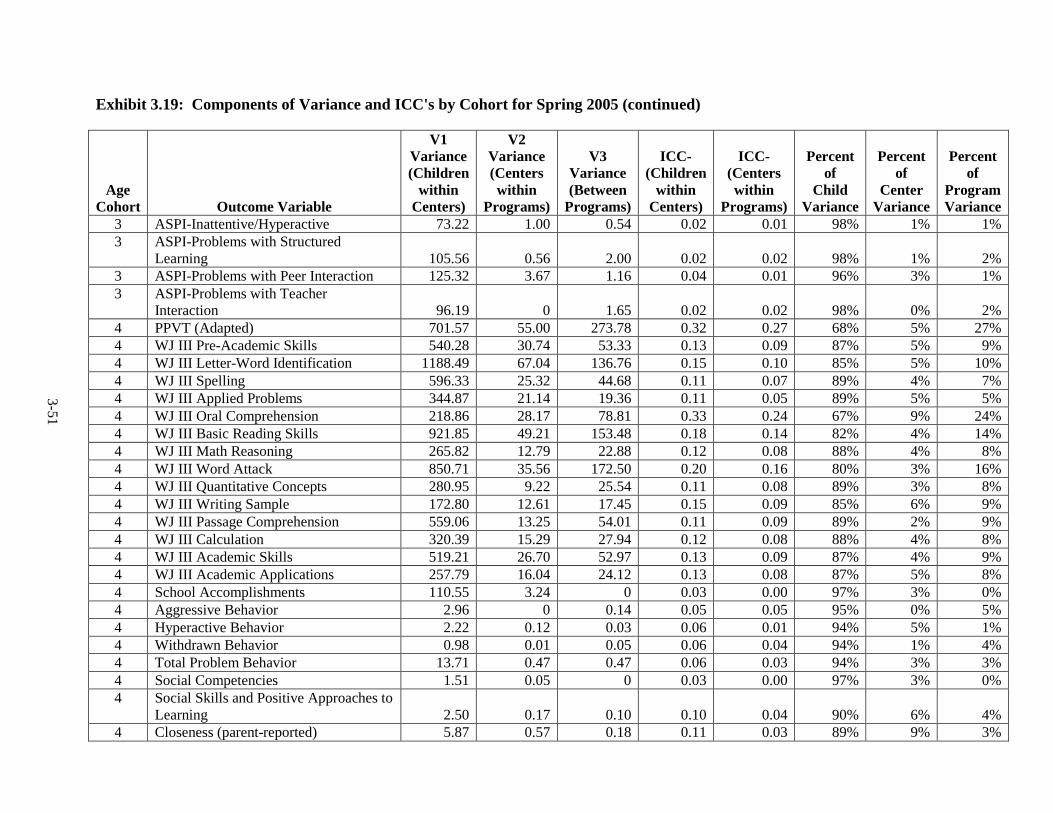
3-51
Exhibit 3.19: Components of Variance and ICC's by Cohort for Spring 2005 (continued)
Age Cohort Outcome Variable
V1 Variance (Children
within Centers)
V2 Variance (Centers within
Programs)
V3 Variance (Between
Programs)
ICC- (Children
within Centers)
ICC-(Centers within
Programs)
Percent of
Child Variance
Percent of
Center Variance
Percent of
Program Variance
3 ASPI-Inattentive/Hyperactive 73.22 1.00 0.54 0.02 0.01 98% 1% 1% 3 ASPI-Problems with Structured
Learning 105.56 0.56 2.00 0.02 0.02 98% 1% 2% 3 ASPI-Problems with Peer Interaction 125.32 3.67 1.16 0.04 0.01 96% 3% 1% 3 ASPI-Problems with Teacher
Interaction 96.19 0 1.65 0.02 0.02 98% 0% 2% 4 PPVT (Adapted) 701.57 55.00 273.78 0.32 0.27 68% 5% 27% 4 WJ III Pre-Academic Skills 540.28 30.74 53.33 0.13 0.09 87% 5% 9% 4 WJ III Letter-Word Identification 1188.49 67.04 136.76 0.15 0.10 85% 5% 10% 4 WJ III Spelling 596.33 25.32 44.68 0.11 0.07 89% 4% 7% 4 WJ III Applied Problems 344.87 21.14 19.36 0.11 0.05 89% 5% 5% 4 WJ III Oral Comprehension 218.86 28.17 78.81 0.33 0.24 67% 9% 24% 4 WJ III Basic Reading Skills 921.85 49.21 153.48 0.18 0.14 82% 4% 14% 4 WJ III Math Reasoning 265.82 12.79 22.88 0.12 0.08 88% 4% 8% 4 WJ III Word Attack 850.71 35.56 172.50 0.20 0.16 80% 3% 16% 4 WJ III Quantitative Concepts 280.95 9.22 25.54 0.11 0.08 89% 3% 8% 4 WJ III Writing Sample 172.80 12.61 17.45 0.15 0.09 85% 6% 9% 4 WJ III Passage Comprehension 559.06 13.25 54.01 0.11 0.09 89% 2% 9% 4 WJ III Calculation 320.39 15.29 27.94 0.12 0.08 88% 4% 8% 4 WJ III Academic Skills 519.21 26.70 52.97 0.13 0.09 87% 4% 9% 4 WJ III Academic Applications 257.79 16.04 24.12 0.13 0.08 87% 5% 8% 4 School Accomplishments 110.55 3.24 0 0.03 0.00 97% 3% 0% 4 Aggressive Behavior 2.96 0 0.14 0.05 0.05 95% 0% 5% 4 Hyperactive Behavior 2.22 0.12 0.03 0.06 0.01 94% 5% 1% 4 Withdrawn Behavior 0.98 0.01 0.05 0.06 0.04 94% 1% 4% 4 Total Problem Behavior 13.71 0.47 0.47 0.06 0.03 94% 3% 3% 4 Social Competencies 1.51 0.05 0 0.03 0.00 97% 3% 0% 4 Social Skills and Positive Approaches to
Learning 2.50 0.17 0.10 0.10 0.04 90% 6% 4% 4 Closeness (parent-reported) 5.87 0.57 0.18 0.11 0.03 89% 9% 3%
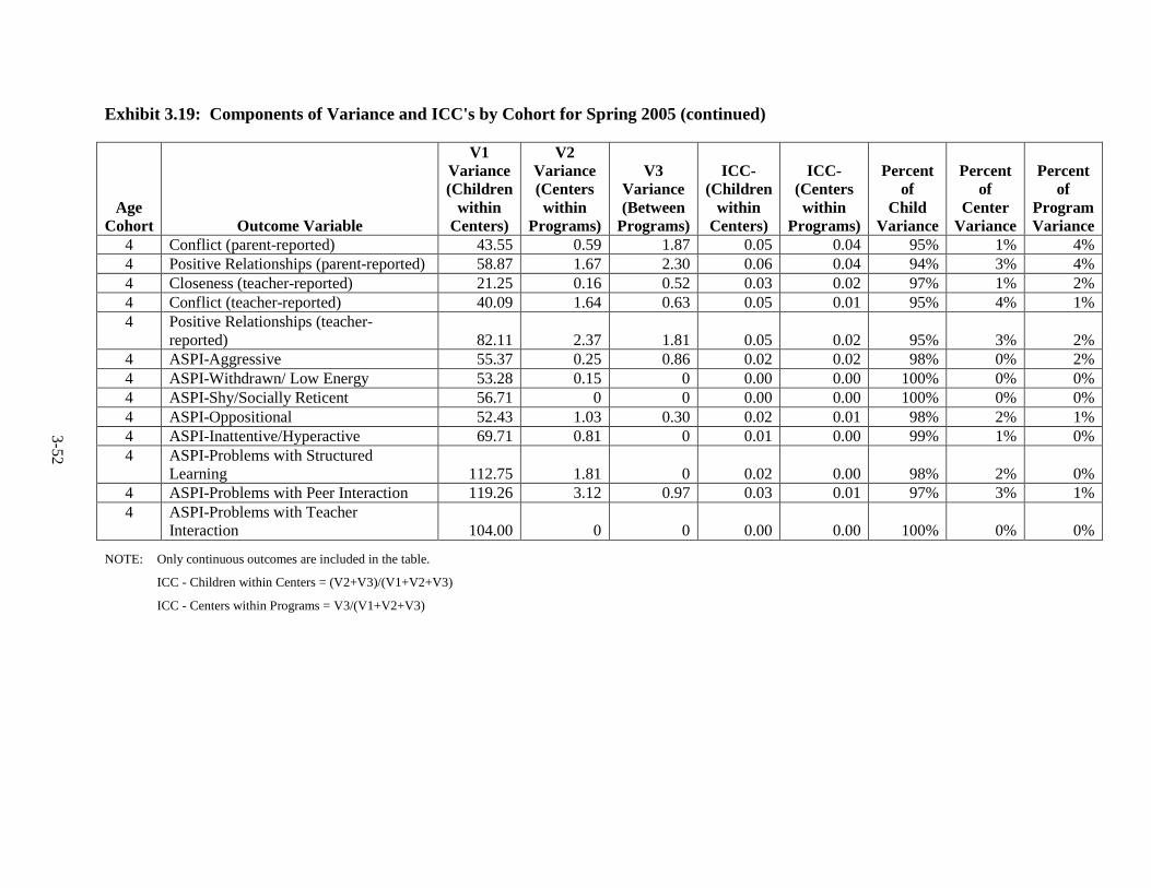
3-52
Exhibit 3.19: Components of Variance and ICC's by Cohort for Spring 2005 (continued)
Age Cohort Outcome Variable
V1 Variance (Children
within Centers)
V2 Variance (Centers within
Programs)
V3 Variance (Between
Programs)
ICC- (Children
within Centers)
ICC-(Centers within
Programs)
Percent of
Child Variance
Percent of
Center Variance
Percent of
Program Variance
4 Conflict (parent-reported) 43.55 0.59 1.87 0.05 0.04 95% 1% 4% 4 Positive Relationships (parent-reported) 58.87 1.67 2.30 0.06 0.04 94% 3% 4% 4 Closeness (teacher-reported) 21.25 0.16 0.52 0.03 0.02 97% 1% 2% 4 Conflict (teacher-reported) 40.09 1.64 0.63 0.05 0.01 95% 4% 1% 4 Positive Relationships (teacher-
reported) 82.11 2.37 1.81 0.05 0.02 95% 3% 2% 4 ASPI-Aggressive 55.37 0.25 0.86 0.02 0.02 98% 0% 2% 4 ASPI-Withdrawn/ Low Energy 53.28 0.15 0 0.00 0.00 100% 0% 0% 4 ASPI-Shy/Socially Reticent 56.71 0 0 0.00 0.00 100% 0% 0% 4 ASPI-Oppositional 52.43 1.03 0.30 0.02 0.01 98% 2% 1% 4 ASPI-Inattentive/Hyperactive 69.71 0.81 0 0.01 0.00 99% 1% 0% 4 ASPI-Problems with Structured
Learning 112.75 1.81 0 0.02 0.00 98% 2% 0% 4 ASPI-Problems with Peer Interaction 119.26 3.12 0.97 0.03 0.01 97% 3% 1% 4 ASPI-Problems with Teacher
Interaction 104.00 0 0 0.00 0.00 100% 0% 0%
NOTE: Only continuous outcomes are included in the table.
ICC - Children within Centers = (V2+V3)/(V1+V2+V3)
ICC - Centers within Programs = V3/(V1+V2+V3)
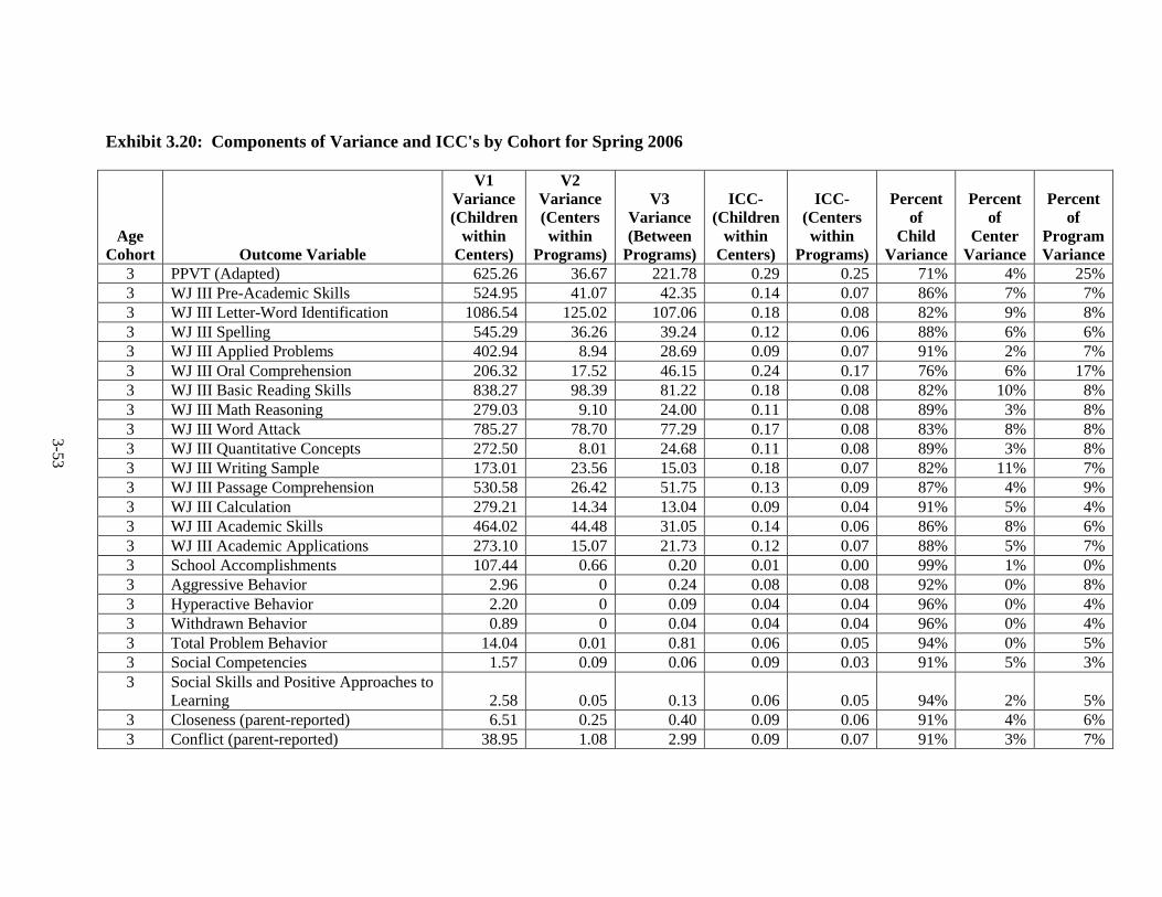
3-53
Exhibit 3.20: Components of Variance and ICC's by Cohort for Spring 2006
Age Cohort Outcome Variable
V1 Variance (Children
within Centers)
V2 Variance (Centers within
Programs)
V3 Variance (Between
Programs)
ICC- (Children
within Centers)
ICC-(Centers within
Programs)
Percent of
Child Variance
Percent of
Center Variance
Percent of
Program Variance
3 PPVT (Adapted) 625.26 36.67 221.78 0.29 0.25 71% 4% 25% 3 WJ III Pre-Academic Skills 524.95 41.07 42.35 0.14 0.07 86% 7% 7% 3 WJ III Letter-Word Identification 1086.54 125.02 107.06 0.18 0.08 82% 9% 8% 3 WJ III Spelling 545.29 36.26 39.24 0.12 0.06 88% 6% 6% 3 WJ III Applied Problems 402.94 8.94 28.69 0.09 0.07 91% 2% 7% 3 WJ III Oral Comprehension 206.32 17.52 46.15 0.24 0.17 76% 6% 17% 3 WJ III Basic Reading Skills 838.27 98.39 81.22 0.18 0.08 82% 10% 8% 3 WJ III Math Reasoning 279.03 9.10 24.00 0.11 0.08 89% 3% 8% 3 WJ III Word Attack 785.27 78.70 77.29 0.17 0.08 83% 8% 8% 3 WJ III Quantitative Concepts 272.50 8.01 24.68 0.11 0.08 89% 3% 8% 3 WJ III Writing Sample 173.01 23.56 15.03 0.18 0.07 82% 11% 7% 3 WJ III Passage Comprehension 530.58 26.42 51.75 0.13 0.09 87% 4% 9% 3 WJ III Calculation 279.21 14.34 13.04 0.09 0.04 91% 5% 4% 3 WJ III Academic Skills 464.02 44.48 31.05 0.14 0.06 86% 8% 6% 3 WJ III Academic Applications 273.10 15.07 21.73 0.12 0.07 88% 5% 7% 3 School Accomplishments 107.44 0.66 0.20 0.01 0.00 99% 1% 0% 3 Aggressive Behavior 2.96 0 0.24 0.08 0.08 92% 0% 8% 3 Hyperactive Behavior 2.20 0 0.09 0.04 0.04 96% 0% 4% 3 Withdrawn Behavior 0.89 0 0.04 0.04 0.04 96% 0% 4% 3 Total Problem Behavior 14.04 0.01 0.81 0.06 0.05 94% 0% 5% 3 Social Competencies 1.57 0.09 0.06 0.09 0.03 91% 5% 3% 3 Social Skills and Positive Approaches to
Learning 2.58 0.05 0.13 0.06 0.05 94% 2% 5% 3 Closeness (parent-reported) 6.51 0.25 0.40 0.09 0.06 91% 4% 6% 3 Conflict (parent-reported) 38.95 1.08 2.99 0.09 0.07 91% 3% 7%
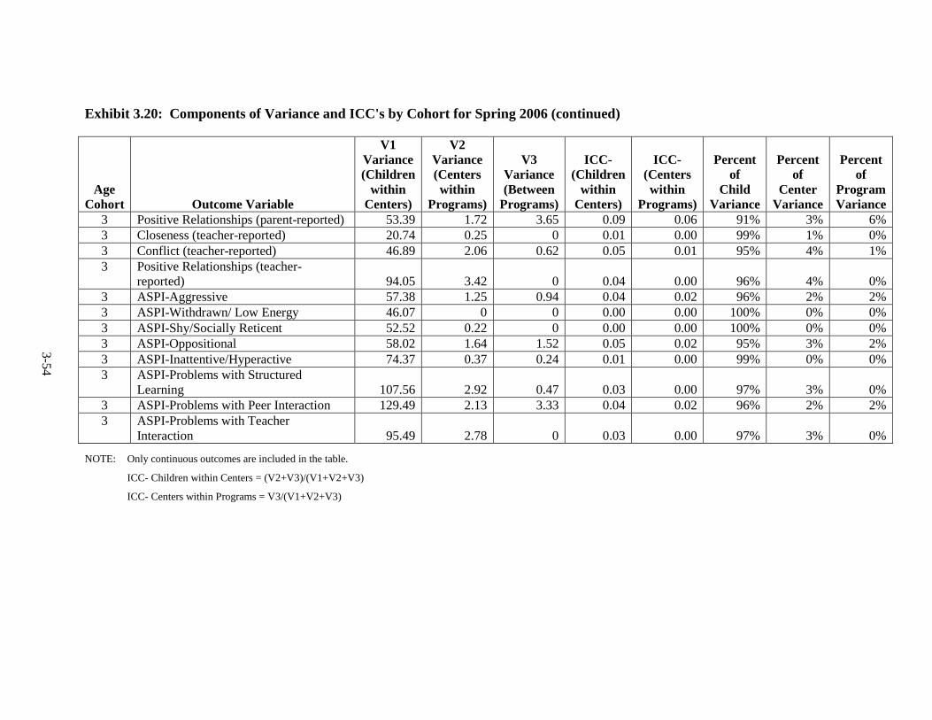
3-54
Exhibit 3.20: Components of Variance and ICC's by Cohort for Spring 2006 (continued)
Age Cohort Outcome Variable
V1 Variance (Children
within Centers)
V2 Variance (Centers within
Programs)
V3 Variance (Between
Programs)
ICC- (Children
within Centers)
ICC-(Centers within
Programs)
Percent of
Child Variance
Percent of
Center Variance
Percent of
Program Variance
3 Positive Relationships (parent-reported) 53.39 1.72 3.65 0.09 0.06 91% 3% 6% 3 Closeness (teacher-reported) 20.74 0.25 0 0.01 0.00 99% 1% 0% 3 Conflict (teacher-reported) 46.89 2.06 0.62 0.05 0.01 95% 4% 1% 3 Positive Relationships (teacher-
reported) 94.05 3.42 0 0.04 0.00 96% 4% 0% 3 ASPI-Aggressive 57.38 1.25 0.94 0.04 0.02 96% 2% 2% 3 ASPI-Withdrawn/ Low Energy 46.07 0 0 0.00 0.00 100% 0% 0% 3 ASPI-Shy/Socially Reticent 52.52 0.22 0 0.00 0.00 100% 0% 0% 3 ASPI-Oppositional 58.02 1.64 1.52 0.05 0.02 95% 3% 2% 3 ASPI-Inattentive/Hyperactive 74.37 0.37 0.24 0.01 0.00 99% 0% 0% 3 ASPI-Problems with Structured
Learning 107.56 2.92 0.47 0.03 0.00 97% 3% 0% 3 ASPI-Problems with Peer Interaction 129.49 2.13 3.33 0.04 0.02 96% 2% 2% 3 ASPI-Problems with Teacher
Interaction 95.49 2.78 0 0.03 0.00 97% 3% 0%
NOTE: Only continuous outcomes are included in the table.
ICC- Children within Centers = (V2+V3)/(V1+V2+V3)
ICC- Centers within Programs = V3/(V1+V2+V3)

3-55
Test Publisher Citations Dunn, L.M., Dunn, L.L., and Dunn, D.M. (1997). Peabody picture and vocabulary test, third
edition (PPVT). Circle Pines, MN: American Guidance Service. Dunn, L.M., Padilla, E.R., Lugo, D.E., and Dunn, L.L. (1986). Test de vocabulario en imágenes
peabody (TVIP). Circle Pines, MN: American Guidance Service. FACES Research Team. Color Names and Counting. Modified from the Color concepts and
number concepts tasks in J.M. Mason & J. Stewart (1989), The CAP early childhood diagnostic instrument (prepublication edition), American Testronics.
FACES Research Team. Letter Naming Task. Modified from a test used in the Head Start
Quality Research Center’s (QRC) curricular intervention studies. FACES Research Team. Story and Print Concepts. Modified from the story and print concepts
task in J.M. Mason & J. Stewart (1989), The CAP early childhood diagnostic instrument (prepublication edition), American Testronics.
FACES Research Team. Writing Sample. Modified from the Name writing task in J.M. Mason
& J. Stewart (1989), The CAP early childhood diagnostic instrument (prepublication edition), American Testronics.
Lonigan, D.J., Wagner, R.K., Torgeses, J.K., and Rashotte, C. (2002). Preschool
comprehensive test of phonological & print processing. Unpublished. McCarthy, D. (1970, 1972). McCarthy scales of children’s abilities. San Antonio, TX: The
Psychological Corporation. Roid, G. and Miller, L. (1997). Leiter-R AM battery. Wood Dale, IL: Stoelting Co. Woodcock, R.W., McGrew, K.S., and Mather, N. (2001). Woodcock-Johnson III tests of
achievement. Itasca, IL: Riverside Publishing. Woodcock, R.W., Munoz-Sandoval, A.F. (1996). Batería-R Woodcock-Muñoz pruebas de
aprovechamiento-Revisada. Itasca, IL: Riverside Publishing.

3-56
References Block, J.H. (1965). The child-rearing practices report (CRPR): A set of Q items for the
description of parental socialization attitudes and values. Berkley, CA: University of California at Berkley, Institute of Human Development.
Clay, M. M. (1979). What did I write? Auckland, N.Z.; Exeter, NH: Heinemann. Lutz, M.N., Fantuzzo, J.F., & McDermott, P. (2002). Multidimensional assessment of
emotional and behavioral adjustment problems of low-income preschool children: Development and initial validation. Early Childhood Research Quarterly, 17(3), 338-355.
Mason, J.M., and Stewart, J. (1989). The CAP early childhood diagnostic instrument
(prepublication edition). American Testronics. Mather, N., and Woodcock, R.W. (2001). Woodcock-Johnson III tests of achievement.
Examiner’s manual. Standard and extended batteries. Itasca, IL: Riverside Publishing. Mislevy, R.J. (1991). Randomization-based inference about latent variables from complex
samples. Psychometrika, 56(2), 177-196. Mislevy, R.J., & Bock, R.D. (1983). BILOG: Item analysis and test scoring with binary
logistic models [computer program]. Mooresville, IN: Scientific Software, Inc. Schrank, F.A. and Woodcock, R.W. (2003). WJ III compuscore and profiles program. User’s
manual. Itasca, IL: Riverside Publishing . Stocking, M. L., and Lord, F. M. (1983). Developing a common metric in item response theory.
Applied Psychological Measurement, 7, 201–210. Teale, W.H. (1988). Developmentally appropriate assessment of reading and writing in early
childhood classrooms. Elementary School Journal, 89, 173-183.
U.S. Department of Health and Human Services, Administration for Children, Youth and Families. (2003). Head Start FACES 2000: A whole-child perspective on program performance. Fourth progress report. Washington, DC: Author.

4-1
Chapter 4: Data Collection Procedures
Introduction
Data collection for the Head Start Impact Study began in fall 2002 and continued through
spring 2006, following the same children from age of entry into Head Start through the end of 1st
grade. Comparable data were collected on children and families randomly assigned to both the
Head Start treatment and control groups who were part of both the 3- and 4-year-old study
cohorts.
Data collection focused on the full range of comprehensive services and integrated
program elements for children and their families that form the cornerstone of the Head Start
program and contribute to the child’s readiness for and success in school. Data were collected
from parents, children, Head Start program staff, other child care providers, and teachers; during
the preschool years, observations of classrooms and day care homes were also conducted to
provide direct assessments of the quality of both Head Start and other child care settings.
Comparable data collected for both Head Start and control group children consisted of
the following:
Measures of children’s development that include (1) direct child assessments, (2) parent reports, and (3) teacher/care provider reports. Child outcomes were measured in the key domains of cognitive development (including assessment of skills in the areas of reading, writing, vocabulary, oral comprehension and phonological awareness, and math), social-emotional development, and health.
Characteristics and quality of children’s home environments were measured through (1) parental reports of beliefs and attitudes about their child’s learning and parental participation in, and satisfaction with, their child’s child care experience; (2) family household and demographic information, including parent-child relationships and the quality of the child’s home life; (3) parent ratings of their child’s behavior problems, social skills, and competencies; (4) parents’ perceptions of their child’s accomplishments; (5) parents’ perception of their relationship with their child; and (6) child and family receipt of a variety of comprehensive services.
Characteristics and quality of the primary preschool and child care arrangements were measured through (1) interviews with center-based directors, (2) surveys of teachers or interviews with care providers, and (3) observations of these settings. Characteristics and quality of school settings were measured through (1) surveys of teachers and (2) by linking schools attended by study children to

4-2
annual data collected from every public school in the U.S. by the Department of Education’s National Center for Education Statistics (NCES).
Data collection activities for each wave of data collection are summarized in Exhibits 4-1 and
4-2.
Exhibit 4-1. Data Collection Schedule – 3-Year-Old Cohort 2002-2003
Head Start Year 2003-2004 Age 4 Year
2004-2005 Kindergarten
2005-2006 1st Grade
Fall Spring Fall Spring Fall Spring Fall Spring Children
Parent/Primary Caregivera
Program Staff/Other Care Provider and Elementary School Teacher
Quality of Care Setting a Primary caregiver data collection in fall ’03, 04, and 05, is limited to tracking and confirming the following spring
school setting. Exhibit 4-2. Data Collection Schedule – 4-Year-Old Cohort 2002-2003
Head Start Year 2003-2004
Kindergarten 2004-2005 1st Grade
2005-2006 2nd Grade
Fall Spring Fall Spring Fall Spring Fall Spring Children
Parent/Primary Caregivera
Program Staff/Other Care Provider and Elementary School Teacher
Quality of Care Setting a Primary caregiver data collection in fall ’03, 04, and 05, is limited to tracking and confirming the following spring
school setting.

4-3
Data Collection Staff Structure
Highly experienced and skilled teams of professional researchers, field supervisory staff,
and field interviewer/assessors, and classroom observers implemented a comprehensive data
collection plan to complete all recruitment, random assignment, data collection, and monitoring/
quality control tasks. Beginning in February 2002, recruitment teams, comprised of senior staff,
visited each of the sampled Head Start grantees to enlist program cooperation and participation
in the study, and to gather information needed to design random assignment and monitoring
procedures, and to gain insight on the state and local context within which the Head Start
programs operated. In addition, during data collection, some individuals from these recruitment
teams conducted quality control visits and continued responsibility in ensuring elementary
school participation as the study children started their early school years.
The critical efforts of these recruitment teams were supplemented by those of local
Westat field supervisors, called “site coordinators,” who were assigned to a geographic area
immediately after sample selection, with many continuing in this role for the duration of the
study. The site coordinator’s role was a pivotal one in serving as the primary local contact. Site
coordinators often laid the groundwork and helped with the preparation for the recruitment team
visits, and later with providing additional information and follow-up (e.g., conducting
parent/primary caregiver meetings and community meetings to respond to questions or concerns
after the recruitment teams’ visits).
After each grantee was successfully enrolled in the study, the recruitment teams and site
coordinators worked with program administrators to select a program staff person to serve as the
“on-site liaison” to work closely with the site coordinator. On-site liaisons and site coordinators
worked hand in hand to: implement random assignment; recruit and maintain the cooperation of
study participants including parents and their children, teachers, and administrative staff; secure
informed consent from parents; make all logistical arrangements for data collection; and assist
with tracking study participants over time. These relationships, developed early in the course of
the study, were invaluable in ensuring open communications, achieving cooperation and
participation, and developing trusting, ongoing working relationships with the sites.
Following the completion of random assignment, and obtaining informed consent from
parents, local measurement teams, comprised of interviewer/assessors and observers, under the

4-4
supervision of the field site coordinator, completed the various data collection tasks in each of
the 25 geographic areas that comprised the study sample for each data collection wave. These
data collection tasks included conducting in-person parent interviews, individual child
assessments, and distributing and collecting self-administered staff questionnaires. During the
preschool years, teams of specially trained observers were responsible for conducting Head Start
and non-Head Start classroom and day care home observations to provide assessments of
program quality, and site coordinators also conducted interviews with both Head Start and non-
Head Start center directors. Throughout the successive waves of data collection, the site
coordinators continued to coordinate all data collection activities in the geographic area; tracking
study participants; managing field staff, and ensuring quality control.
Staff Training
Beginning in fall 2002, and then each spring thereafter through spring 2006, a single
centralized in-person training was conducted in the Washington, DC area for all field
interviewer/assessors and site coordinators. At each of the trainings, Westat field staff were
trained thoroughly in the administration of all data collection instruments for that wave including
administering the child assessment, conducting the parent interview, fielding the self-
administered teacher survey and teacher’s/care provider’s child report form (TCR), and
conducting the center director interview. Field staff also were trained in all field procedures
including securing parent participation, obtaining informed consent, tracking respondents,
building rapport, maintaining cooperation over time, and conducting refusal conversion. This
centralized in-person approach ensured standardization of methods and procedures, fostered
camaraderie and a shared sense of purpose, and enabled the Project Officer and other federal
staff to easily attend.
In addition, for the fall parent updates, telephone conference trainings were conducted on
the parent tracking update with a followup telephone conference question and answer session
one week later. Then, site coordinators provided additional training for their interviewer/
assessors and also corrective feedback immediately after conducting an edit of the first few
instruments.
Also, during each of the first two years of the study, separate centralized in-person
training sessions were conducted in the Washington, DC area for field staff observers to train

4-5
them in conducting classroom observations in Head Start and other center-based programs.
Observers received in-depth training in using a structured classroom observation instrument
comprised of a table to record counts of children and adults, a Classroom Observation of
Teacher-Directed Activities, the Early Childhood Environment Rating Scale – Revised (ECERS-
R), and the Arnett Scale of Lead Teacher Behavior. Training included multiple practice
observations in local classrooms, followed by small group interactive training sessions to achieve
and ensure the required high degree of reliability. Separate trainings were also conducted to
prepare observers to conduct observations in day care homes, substituting the Family Day Care
Rating Scale (FDCRS) for the ECERS-R.
For every year of data collection, these training sessions lasted at least five days and as
many as nine days, depending upon the data collection tasks for that round of data collection.
Given that over time much of the field staff was experienced on the study, and some were with
the study since its beginning in fall 2002, the trainings could be structured to include fewer days
for experienced returning staff than for new staff. The trainings enabled new staff to benefit
enormously from the experienced staff who shared their successful methods and ideas, both in
large group training sessions and in the small group interactive practice sessions where we
deliberately paired each new staff member with a returning staff member to foster peer learning.
New staff attended a one-day preliminary session to provide an introduction to general
interviewing techniques and afford an opportunity for experience and practice with the
instruments prior to the main combined training conducted over several days for all field staff.
Site coordinators also participated in a separate preliminary set of training sessions led by
home office staff. These sessions were geared to developing the management, leadership, and
computer skills necessary to the site coordinators’ assignments including supervising the
interviewer/assessors, overseeing the logistical procedures, and coordinating data collection. In
addition to the training they received from the operations director, field director, and other home
office staff, site coordinators attended workshops structured for them to share their ideas and
successful techniques with each other and with their managers. In addition, time was scheduled
for the new interviewer/assessors and their site coordinators to meet and discuss project goals
and expectations.

4-6
A variety of methods were employed such as interactive large group sessions including
video and live demonstrations of assessment administration to provide an overview and detailed
training on the various segments of the instruments including rules for administration, coding
and scoring, engaging respondents, and providing “neutral praise” that provides encouragement
without reacting to the particular response or level of achievement (e.g., “you’re doing such a
nice job of cooperating”). Small group breakout sessions also were included with round robin
practice of the entire assessment and key sections as well as role plays to gain familiarity and
proficiency with the instruments. One day of training was devoted to live practice of the child
assessment with children with evaluation and corrective feedback provided. Additional evening
training sessions also were conducted to provide further training and practice for those who
wanted it and those for whom the trainers felt it was necessary.
Additional training sessions and practice with instruments in Spanish was required for the
bilingual English/Spanish interviewer/assessors. Experienced bilingual project staff conducted
these sessions tailored to the administration of parent interviews and child assessments in
Spanish.
Training materials included an agenda of project activities, an interviewer/assessor’s
manual and training scripts and exercises. The materials were customized for each round of data
collection and provided a framework for training, a set of valuable reference materials for staff in
the field, and documentation of the procedures and content used during the administration of the
instruments. Interviewer/assessors also completed a half day of home study following training to
enhance learning from the in-person sessions.
Interviewer/assessors and observers were trained to strictly follow procedures, read
questions verbatim, provide “neutral praise” to respondents and adhere to study protocols to
ensure that the highest quality data were collected without biasing responses. Practicing the
child assessment with an adult partner is quite different from conducting an assessment with an
actual child. To ensure high quality, every interviewer/assessor was required to demonstrate
proficiency in the child assessment by conducting the assessment with a child of the same age as
the study children. We recruited children from the local Washington, DC area to serve as
practice subjects at training and found this to be a highly effective tool to gauge interviewer/
assessors’ proficiency in administering the child assessment. Only interviewer/assessors who

4-7
passed the child assessment live practice session were permitted to conduct child assessments in
the field. Similarly, observers visited schools recruited in the local Washington, DC area as
training sites for observers to observe and develop inter-rater reliability.
Informed Consent
To secure the cooperation of parents, a complete package of materials and advance
publicity was designed to inform potential participants and enlist their participation as early as
possible. The materials explained that the grantee was participating in a study and that applying
meant that the caregiver was agreeing to random assignment procedures. Separate informed
consent was obtained to participate in subsequent data collection (described below). These
materials enlightened parents (prior to and/or during the application process) regarding the key
elements and benefits of the study; notified them of the various incentives that would be
provided for their cooperation over time, and informed them of their role in completing
interviews and aiding study staff in locating and securing the participation of child care
providers. Recruitment teams and site coordinators met with grantees, parents, and staff to
explain critical information to potential participants; highlight reasons to participate in the study;
explain the process and importance of random assignment for the study design; and describe the
implications of this process for children and families assigned to the treatment and control
groups.
Following random assignment in late summer and early fall 2002, parents were
immediately contacted to notify them of their selection, and to secure written informed consent.
At the outset, consent was obtained for the duration of the study with parents agreeing to their
child’s participation and assessment, as well as to allowing the study team to contact their child’s
care providers/teachers to gain their cooperation, and to obtain important locator and tracking
information to help locate the family in the future, particularly if the family moved. Site
coordinators met with the parents/primary caregivers in group settings, (e.g., in Head Start and
other child care centers when feasible), and individually as necessary, to explain the study,
respond to questions, read the informed consent letters as necessary, and obtain the
parents’/primary caregivers’ signed informed consent. Field staff used a number of aids to
inform parents, encourage their participation, and gain informed consent including a script with a
brief statement explaining the purpose and importance of the study and a description of the

4-8
information to be collected, assurances that participation is voluntary and information collected
will be kept private, and a description of the cash incentive; a study brochure and a study
information sheet with frequently asked questions and answers; as well as procedures to guide
the determination of whether the person contacted is the parent/primary caregiver, and therefore,
the appropriate respondent.
The informed consent letters summarized the purpose, scope, and importance of the study
and described the activities as well as the incentives for participating. The letters included a
statement that participation is voluntary and an assurance that respondents’ participation would
not result in a loss of any current benefits they might have. The letters also included an
assurance of privacy. We used several approaches that enhanced our ability to secure parents’
consent and gain continued participation of families. These included incentives for participation,
assurances of privacy, and an emphasis on the importance of parents’ sharing their experience to
further improve early childhood programs. For those from whom consent was not obtained prior
to the start of data collection in fall, field staff obtained informed consent in person prior to
conducting the parent interviews or child assessments in fall or spring. Securing blanket
informed consent at the outset of the study was a major step toward maintaining high response
rates.
Field interviewers/assessors and site coordinators were thoroughly trained in strategies
for gaining and maintaining cooperation. Field staff members were trained in identifying,
understanding, and responding appropriately and effectively to reasons why parents may be
hesitant to cooperate. They were taught strategies to reassure the parents and ensure their
cooperation including efforts to find out why the respondent was reluctant and to address these
concerns wherever possible. Just as one respondent differs from another, the reasons for refusals
are many and varied so it was necessary to train field staff to become sensitive to how firm a
“no” they are receiving and sense the reasons behind the hesitancy to develop ways to reassure
the respondent and gain cooperation.

4-9
Data Collection Procedures by Respondent
Collecting Parent/Primary Caregiver Data
Beginning with baseline in fall 2002, and then each spring thereafter until the child’s 1st
grade year, interviewer/assessors conducted face-to-face interviews, approximately one-hour in
length, with a parent/primary caregiver living with and responsible for raising the study children.
Questions were included to obtain information about the characteristics and involvement of other
family members as well. Interviews typically were conducted in the family’s home, or
alternatively, if the parent preferred, in a suitable public location such as a library.
In addition, to keep the families actively involved and to continue to track the families
effectively, each fall beginning in fall 2003, site coordinators and interviewer/assessors
conducted short telephone, and when necessary, in-person parent update interviews, collecting
tracking information and the child’s current school and/or care setting information to provide a
basis for the spring data collection. We used a number of approaches to strengthen and maintain
the parents’ commitment to continuing in the study. These included: maintaining frequent in
person, telephone and mail contact with the families coupled with providing monetary
incentives.
Parent interviews were conducted in the languages of the respondents and were available
in both English and Spanish versions. Bilingual interviewers were hired and for most of the
languages, including Spanish, Creole, Cantonese, etc., interviewers fluent in the language
conducted the interview. When this was not the case, we enlisted the aid of an interpreter to
assist an English-speaking interviewer trained to conduct the interview.
Collecting Child Assessment Data
Children were assessed individually in fall 2002 and then each spring through 1st grade
using a battery of child measures (see Chapter 3 in this volume). The assessments were designed
to provide direct measures of how well Head Start and non-Head Start preschool programs, or
other child care, are achieving the goal of assisting children to be physically, socially, and
educationally ready for school. The assessment battery was composed of a short series of tasks
that varied over time consistent with the child’s age. Children who did not advance to the next

4-10
level of schooling with their peers, or who were advanced, continued to be assessed with the
instruments for their cohort group.
During the preschool years, the 45 - 60 minute child assessment battery was typically
administered one-on-one by specially trained assessors in the child’s “main” care setting, i.e.,
where the child spends the most time Monday through Friday between the hours of 9 a.m. and
3 p.m. When the children attained school age, the assessments were typically conducted in the
child’s home or if the parent preferred, in a suitable public place.
To determine the appropriate language of assessment, at the time of baseline in fall 2002,
the interviewer/assessor asked the main care provider a series of three questions (see Chapter 3).
For children for whom Spanish was the appropriate language, a bilingual interviewer/assessor
administered the assessment battery in Spanish and also administered two subtests in English,
i.e., the Peabody Picture Vocabulary Test (adapted) (PPVT) and the Woodcock-Johnson III
Letter-Word Identification. Subsequently, each spring, the children assessed in Spanish in fall
2002 were assessed primarily in English, along with the continued administration of two Spanish
language measures: the Test de Vocabulario en Imágenes Peabody (TVIP) and the Batería
Woodcock-Muñoz Identificación de Letras y Palabras. One exception is Puerto Rico where,
because instruction is in Spanish, all children were assessed only with the complete Spanish
battery each spring for the duration of the study.
In fall 2002, for children who could not be assessed in either English or Spanish, a
bilingual interviewer/assessor or an interpreter for the child’s language were used. The
interviewer/assessor (or interpreter) used the English assessment booklet, translated the
instructions into the child’s language, and administered four subtests: McCarthy Draw-A-
Design, Color Names and Counting, Leiter-R-Adapted, and Story and Print Concepts. These
four tests do not require the child to be able to speak English. Those subtests that would require
the child to speak English were not administered to this population. Subsequently, for the spring
assessments, these children were tested in English.
Collecting Data from Program Staff, Teachers and Child Care Providers
During the preschool years, Head Start and preschool program teachers as well as other
child care providers (other than parents/other primary caregivers) were surveyed each spring, and

4-11
center directors were also interviewed on an annual basis. During the elementary school years,
kindergarten and 1st grade teachers were surveyed, again in the spring. Parents and primary
caregivers played a key ongoing role in identifying the child’s care providers and granting
permission for us to contact them. Parents were offered additional incentive payments for
contacting the child care providers and securing their cooperation. Providers who participated
also were offered a monetary incentive.
Both preschool and elementary school teachers completed self-administered paper
questionnaires including a teacher survey, as well as an individual child rating form, the
teacher’s/care provider’s child report (TCR) for each study child in the teacher’s class. Only the
lead teacher in the study child’s classroom was surveyed. The teacher surveys required
approximately 30 minutes and were available in both English and Spanish. The Spanish version
was used largely in Puerto Rico, but also, when necessary on the mainland. The teacher surveys
included questions about the center or school, questions about the class, and questions about the
teacher, and were designed to gather information about school settings, teachers’ beliefs about
how children learn, levels of education, and job satisfaction.
During the preschool years, if the child was not in a center or preschool classroom, but
was cared for by another child care provider other than the parent or primary caregiver, at least
five hours per week between the hours of 8 a.m. and 6 p.m., Monday through Friday, in-person
interviews were conducted requiring approximately 30 minutes with that care provider, and the
care provider was also asked to complete an individual child rating form, the teacher’s/care
provider’s child report (TCR). For children in multiple arrangements that met these criteria, the
following hierarchy was used to prioritize the care setting and within that, the care provider to
interview: (1) day care home with non-relative; (2) day care home with relative; (3) child’s
home with non-relative; and finally, (4) child’s home with non-parental relative. The interview
included questions on the number of children in the care setting, types of child activities used,
beliefs on how children should be taught and managed, options for parent and family
involvement, staffing, and respondent demographic information. While not all of the child’s care
providers were directly interviewed, information was obtained from the parent/primary caregiver
on all the settings in which the child was placed.

4-12
As noted above, teachers and care providers also were asked to complete a TCR. The
TCR is an individual child rating form that asks about the child’s development and behavior.
The following scales are used: teacher/provider relationship with child, classroom behavior and
conduct, problem solving and initiative, social relationships, creative representation, music and
movement, language ability, and mathematical ability. The child rating forms required
approximately five – ten minutes per form and were available in both English and Spanish
versions. A separate booklet was completed by the lead teacher in the child’s classroom or the
care provider each spring during the preschool, kindergarten and first grade years.
During the preschool years, both Head Start and non-Head Start center directors were
interviewed in person to obtain information on the operation and quality of Head Start and non-
Head Start center-based programs. Issues addressed in this interview included: staffing and
recruitment, teacher education initiatives and staff training, parent involvement, curriculum,
classroom activities and assessment, home visits, kindergarten transition, and demographic
information about the director.
Assessment of Quality of Care Settings
During the preschool years, direct observations of quality and care settings were used for
children in center-based and family day care home programs, including those participating in
Head Start. These tools provided direct measures of the extent to which Head Start centers, and
other childcare programs, employed skilled teachers and provided developmentally appropriate
environments and curricula for their pupils. Trained observers conducted observations in
classrooms and centers attended by the sampled children. Observers spent enough time in each
class to ensure observation of a major portion of the daily schedule and a variety of classroom
and center activities. The observers used standardized observational methods and coding
schemes that have been widely used in child development research and whose utility has been
proven in previous large-scale studies. These include: the Early Childhood Environment Rating
Scale (revised) (ECERS-R), the Classroom Observation of Teacher-Directed Activities
Checklist, the Arnett Scale of Teacher/Provider Behavior, and the related Family Day Care
Rating Scale (FDCRS) for observations in non-center-based settings.
Children were exposed to a wide variety of types of care settings selected by their parents
in addition to, or in lieu of, Head Start. Consequently, it was necessary to arrive at a means of

4-13
carefully targeting and limiting the number of care settings to be assessed to a maximum of one
per child with priority given to those programs where the child was in care at least five hours per
week between the hours of 8 a.m. to 3 p.m., Monday through Friday. For the Head Start group,
Head Start (regardless of full day or part day) was considered the primary setting assessed or the
“focal” setting. For all others, the following hierarchy was used: (1) center-based program,
(2) day care home with non-relative; (3) day care home with relative; (4) child’s home with non-
relative; and finally, (5) child’s home with non-parental relative. While children may spend
significant portions of their time in care settings other than those being assessed for quality, and
these may contribute in important ways to the child’s experience and growth, information on
these settings was obtained solely from the parent interview.
Classroom observations were not conducted in elementary schools, but instead
information on school quality was collected from the teacher questionnaire, (e.g., years of
teaching experience, years of schooling, number of hours of in-service training), and through
secondary data sources (e.g., percent of children eligible for free or reduced-price lunch, percent
of children in the children’s schools who scored at the “proficient level” on state math and
reading assessments, class-size ratio, etc.).
Privacy
Protecting and maintaining the privacy of respondents and their data were primary
concerns and were treated very seriously. Parent/primary caregiver respondents received
assurances that “all information collected during the study will be kept private except as required
by law.” This assurance was included in the informed consent letters the parents/primary
caregivers signed to participate in the study, and was reiterated in the letters they received to
announce the beginning of each data collection period with similar statements incorporated in the
parent interviews. Teachers and administrators also received assurances of confidentiality.
Included in the cover letters for the teacher questionnaires was this statement: “All responses are
treated with strict confidentiality and members of the study team are committed to this. To
ensure confidentiality, survey results will not be reported for any individuals, agencies, centers,
preschool programs, child care providers, or schools.” In addition, the Head Start Impact Study
“Study Information Sheet,” distributed to parents and other respondents to answer some
frequently asked questions included this assurance: “The confidentiality of each participant is

4-14
carefully protected under federal law. No information will be linked to a specific child, parent,
or staff member. No information will be released about individuals or child care providers. All
information will be held in strict confidence and will be protected.”
Staff were required to sign a confidentiality pledge stating that no data would be released
to unauthorized personnel. All field data collectors were required to sign Westat’s Fieldworker
Code of Conduct and Assurance of Confidentiality form prior to each data collection period.
Protecting and maintaining confidentiality of respondent data was also a topic covered in depth
in the training manual and at interviewer training to have interviewers understand and apply
ethical principles and practices when conducting their work, provide historical context, and raise
interviewers’ awareness of the importance of informed consent and confidentiality. Any
interviewers found to violate confidentiality are subject to immediate dismissal as described in
the Fieldworker Employee Guide. In addition, all Westat home office professional staff were
required to take Westat’s online course on the protection of human subjects. This online course
emphasizes the protection of respondents as human subjects and the serious obligation of
protecting the confidentiality of respondent data. Quality control monitors and site coordinators
reinforced and enforced confidentiality standards and instructions in the field. A special version
of the online course that includes computer data security procedures was required study for all
programming staff.
Access to Westat facilities is controlled at all times through the use of magnetic key
cards. Access to the computer centers is also controlled by the key card entry system, with
limited access privileges for designated operations and project support staff only. Special
secured areas are established for sensitive data processing functions such as storing and printing
of confidential data based on project requirements.
Data collected in hard-copy form are kept in a locked field room accessible only by
authorized project staff. Signs restricting access are posted at the entrances to secured data
processing areas. Likewise, system-generated output containing confidential data is stored in
locked areas until no longer needed and is disposed of in accordance with project requirements.
Access to secure computer systems is password protected with all electronic data (including
records with identifying information) stored on password-protected servers and accessible only
by authorized research and programming staff.

4-15
Several steps are taken to prevent the loss or corruption of data in case of equipment or
facility failure. First, users are instructed to store all data files on network server directories
rather than local PC hard disk drives. Second, Westat’s Computer Operations staff backup all
server-based storage to tape on a daily basis as well as performing a full disk backup once a
week with an additional backup created every fourth week and retained for one year. All backup
tapes are removed daily from Westat’s premises and transported in secure containers to an off-
site storage facility that specializes in transporting and storing electronic media. Tape identifiers
for all backup tapes are maintained in a central tape management system for easy reference and
retrieval.
Interviewers agree to keep all case record folders with names and addresses and all
instruments in a secure place in their home. While in the field they are required to keep all study
materials with them at all times.
Interviewer/assessors and site coordinators are also trained on proper procedures to
communicate confidential information securely, including using ID numbers instead of
respondent names in email messages and password protecting files that contain respondent
names and addresses. Field staff returned hard copy completed instruments to the home office
via Federal Express. All completed hard-copy instruments are kept in a locked field room
accessible only by authorized project staff. Data that are transmitted are encrypted before being
transmitted to the home office so that all data are secure and cannot be accessed even if the data
were intercepted in the transmission. All electronic data (including records with identifying
information) are stored on password-protected servers and accessible only by authorized research
and programming staff.
Westat further protects the privacy of families by making sure that interviewer/assessors
do not interview families whom they know. If interviewer/assessors encounter a family with
whom they are acquainted (other than from a previous round of data collection), the case is
transferred to another interviewer/assessor. In addition, Westat had a policy of not hiring Head
Start staff as interviewer/assessors to minimize the likelihood of previous acquaintance with
study families.
4-16
Incentives
Incentives provided a valuable and effective mechanism for encouraging parents/primary
caregivers, children, teachers, and other care providers to participate initially and to maintain that
participation throughout the longitudinal study. For this study, the children received small gifts
including stickers, notepads, and pencil sharpeners following their completion of the child
assessments. Parents/primary caregivers received $20 in cash following each in-person
interview, along with an additional bonus payment during the last round of data collection of $25
if the family participated in all previous rounds of data collection. Parents received a check or
money order for $20 for the short tracking telephone update. These incentives encourage
cooperation and participation, emphasize the importance of the study and underscore the value of
respondents’ participation in it.
Teacher incentives also proved to be very effective and consisted of a graduated cash
incentive for completing the teacher survey and TCRs depending on the number of child forms
completed: $15 for the teacher survey and 1-3 child forms; $25 for the survey and 4-10 child
forms; or $35 for the survey and 11+ child forms. Most teachers received an incentive of $15.
For classroom and day care home observations, center directors and day care home providers
received a check in the amount of $25. Incentives were not offered for the center director
interview, as a high level of cooperation was obtained without offering an additional incentive
for interviewing administrators at this level.
Tracking
Tracking is a critically important part of a longitudinal study such as the Head Start
Impact Study. Once a child is selected into the study, the child remains in the study, and
consequently, must be traced throughout the course of the study. The collection of data other
than the parent interviews was, however, limited for cost purposes to all children who remained
in their original area or who moved within a 50-mile radius of the sampled Head Start centers.
When a family moved to the geographic area of another site, the case was transferred for
purposes of completing data collection there. Staff continued to trace children regardless of how
far away they moved, and when the family was located outside the 50-mile radius of any of our
sites, the parent interview was conducted by telephone when possible. Although families may
4-17
move far away from an area, they frequently return, and therefore, despite the fact that we may
not have complete data for all waves of data collection, we did endeavor to collect data from
families during as many waves as possible.
Initial contact information was obtained for the parent/primary caregiver from the Head
Start program applications submitted for admission to Head Start in fall 2002. Interviewers/
assessors and site coordinators updated contact information supplied by the parent/primary
caregiver during each round of data collection in the spring parent interview and during the fall
parent update. Maintaining contact with families twice a year to update contact information for
the parent/primary caregiver and up to three contacts proved a very effective strategy both for
maintaining parents’ interest and participation in the study and for locating and contacting
families in successive rounds. The most recent information was made available to field staff for
the following round of data collection. Field staff were trained in maintaining professionalism
and adhering to the required confidentiality rules while tracing.
If the family could not be reached easily by telephone and a move was suspected, field
staff followed a number of leads, narrowly focused at first and then expanding as needed. Field
staff utilized telephone directory assistance, called the contacts supplied by the parent/primary
caregiver, conducted internet searches, visited the last known address for the family to check
with primary sources in the neighborhood, and when necessary, contacted additional secondary
local sources such as the post office to endeavor to locate the family. When feasible, long
distance tracing efforts were coordinated between teams (i.e., when a family moved to the
geographic region within or close to another study site).
Quality Control
Findings from research are dependent on the quality of the data collected. Therefore,
procedures were built into every step of this national study to ensure the highest quality data
possible. All measures and procedures were reviewed and tested multiple times. Project staff
and field staff were selected based on their skills and experience in conducting this type of
research. To provide a solid base of knowledge and skills necessary to be successful in
collecting the data staff were provided detailed training materials with a consistent set of
definitions and rules as well as substantial opportunities at training for practice in applying these
4-18
rules and definitions. High quality data are the result of well trained and skilled interviewers and
observers.
As noted above, for every year of data collection, intensive in-person trainings were
conducted for as many as nine days, depending upon the data collection tasks for that round.
Additional days of training were provided for new interviewers. Interviewers and observers—
both new and returning—were constantly evaluated during training for their strengths and
weaknesses and extra evening sessions were required for those who needed additional practice.
Out in the field, once the data were collected, interviewer/assessors and observers were
trained to take the next step in the quality control process: reviewing and editing all completed
data collection forms for completeness and clarity. In addition, site coordinators carefully edit
and review the booklets to identify any errors or issues as soon as possible and avoid ongoing
problems. Field staff also are trained to record notes as necessary to explain unusual situations.
When the data collection forms and instruments are received at the home office, they are edited
again by our data processing staff. If necessary, additional coding or scoring also is done at this
time, and site coordinators are contacted to resolve inconsistencies or other questions that arise
during the home office review.
In addition to all of the other quality control measures used on this project, in fall 2002
and each spring thereafter, project staff trainers conducted quality control visits to the sites in the
study. The purpose of these visits was to ensure that field data collectors used and maintained
consistent data collection techniques, administered the instruments accurately, and scored the
instruments correctly and reliably. All new interviewers/assessors and observers and some
returning field staff had quality control visitors. These on site evaluations were invaluable in
correcting small errors before they became ingrained. Inter-rater reliability was monitored
during the training sessions and in the field by quality control visitors.
Response Rates
Response rates are presented in Chapter 2.
5-1
Chapter 5: Impact Analysis Methods
This chapter describes the procedures used to calculate and test the statistical significance
of all estimates of impact on child and parent outcomes presented in the Head Start Impact Study
Final Report (U.S. Department of Health and Human Services, January 2010), providing greater
detail than what readers can find in Chapter 2 of that report. This chapter is organized into nine
sections: Section 1 summarizes all of the outcome measures used in the impact analysis; Section
2 describes the baseline variables used as covariates in the analysis, including imputation for fall
2002 item and instrument nonresponse. Section 3 gives a brief description of the analysis
weights (more detail can be found in Chapter 2); Sections 4 and 6 describe the procedures used
to calculate annual impact estimates both for the full sample and for selected subgroups; Section
5 discusses procedures for calculating “impact on treated (IOT)” estimates, i.e., impact estimates
for those children who actually participated in Head Start; Section 7 describes the methods used
in the longitudinal, repeated measures, analysis to estimate Head Start impacts on children’s
cognitive growth. Finally, Section 8 notes how the analysis methods in this report differ from
those in the previous Interim Report (U.S. Department of Health and Human Services, 2005), for
a small number of situations for which technical improvements were possible.
Outcome Domains and Measures
A wide variety of data sources and measures are used in this report to assess the impact
of Head Start on fostering and enhancing child development, including direct child assessments,
parent/primary caregiver interviews, interviews with providers of early care services used by
participating study children, observations of children’s early care settings, and information
provided by kindergarten and 1st grade teachers. Outcome measures span the cognitive, social-
emotional, parenting, and health domains, as described in Chapter 3. The baseline measures
indicated were collected in fall 2002; outcome information was collected in spring 2003, 2004,
2005, and 2006. Both study cohorts—children who entered Head Start and the research sample
at age 3 and those entering at age 4—were followed through the end of 1st grade; as a result, data
for the older cohort end in spring 2005 while the younger cohort is followed until spring 2006.
Exhibit 5.1 provides a summary of all the outcome measures and a full description of these
measures is found in Chapter 3.

5-2
Exhibit 5.1: Summary of the HSIS Measures by Domain and Data Collection Period
Measure Preschool
Year(s) Kindergarten 1st Grade COGNITIVE
Language and Literacy Peabody Picture Vocabulary Test (PPVT) (Adapted)* X X X Woodcock-Johnson III Letter-Word Identification* X X X Woodcock-Johnson III Spelling* X X X Woodcock-Johnson III Oral Comprehension* X X X Woodcock-Johnson III Pre-Academic Skills* X X X Color Identification* X Preschool Comprehensive Test of Phonological and Print Processing (CTOPPP) Elision* X X Letter Naming X X Woodcock-Johnson III Word Attack X X Woodcock-Johnson III Basic Reading Skills X X Woodcock-Johnson III Academic Applications X Woodcock-Johnson III Academic Skills X Woodcock-Johnson III Passage Comprehension X Woodcock-Johnson III Writing Samples X Spanish Language and Literacy Test de Vocabulario en Imágenes Peabody (TVIP) (Adapted)* X X X Batería Woodcock-Muñoz Identificación de letras y palabras* X X X Pre-writing McCarthy Draw-a-Design* X Parent-Reported Literacy Parent-Reported Emergent Literacy Scale (PELS)* X Math Skills Woodcock-Johnson III Applied Problems* X X X Counting Bears* X Woodcock-Johnson III Quantitative Concepts X X Woodcock-Johnson III Math Reasoning X X Woodcock-Johnson III Calculation X School Performance School Accomplishments X X Promotion (Parent-reported) X X Language and Literacy Ability X X Math Ability X X Social Studies and Science Ability X X

5-3
Exhibit 5.1: Summary of the HSIS Measures by Domain and Data Collection Period (continued)
Measure Preschool
Year(s) Kindergarten 1st Grade SOCIAL-EMOTIONAL
Parent-Reported Aggressive Behavior* X X X Hyperactive Behavior* X X X Withdrawn Behavior* X X X Total Problem Behavior* X X X Social Competencies* X X X Social Skills and Positive Approaches to Learning* X X X Closeness X X X Conflict X X X Positive Relationships X X X Teacher-Reported ASPI-Aggressive X X ASPI-Inattentive/Hyperactive X X ASPI-Withdrawn/ Low Energy X X ASPI-Oppositional X X ASPI-Problems with Peer Interactions X X ASPI-Shy/Socially Reticent X X ASPI-Problems with Structured Learning X X ASPI-Problems with Teacher Interaction X X Closeness X X Conflict X X Positive Relationships X X HEALTH
Parent-Reported Child Received Dental Care* X X X Child Has Health Insurance Coverage* X X X Child’s Overall Health Status Is Excellent/Good* X X X Child Needs Ongoing Care* X X X Child Had Care for Injury Last Month* X X X
PARENTING PRACTICES Parent Spanked Child in Last Week* X X X Parent Used Time Out in Last Week* X X X Parent Read to Child in Last Week* X X X Parental Safety Practices Scale* X X X Family Cultural Enrichment Scale* X X X Parenting Style: Authoritarian+ X X X Parenting Style: Authoritative+ X X X Parenting Style: Neglectful+ X X X Parenting Style: Permissive+ X X X

5-4
Exhibit 5.1: Summary of the HSIS Measures by Domain and Data Collection Period (continued)
Measure Preschool
Year(s) Kindergarten 1st Grade Teacher-Reported School Contact and Communication X X Parent Participation X X
NOTE: * indicates baseline measures. + indicates that the data is only available during the age 4 year for the 3-year-old cohort children. The data is available for all children during the kindergarten and 1st grade years.
Background Measures Used in the Analysis
The background measures of child and family characteristics collected in fall 2002 play
several roles in the analysis. They provide descriptive profiles of the population studied and
serve as covariates in the impact analysis to help explain child-to-child variation in outcomes and
thereby reduce uncertainty in (i.e., increase the statistical precision of) the impact estimates.
They also provide the information needed to form subgroups of Head Start children and families
of special policy interest, such as bilingual children or families in particular racial/ethnic groups
(see section on subgroup analysis). Baseline versions of outcome measures (see Exhibit 5.1)
provide additional explanatory power in the analysis; and time-to-assessment variables can
reduce bias due to unequal maturation of treatment13
Adding Demographic and Time Covariates
and control group children for outcome
measures collected at somewhat different times each spring for the two groups. The following
discussion describes the selection and use of demographic covariates, baseline test scores, and
imputation for item and instrument nonresponse for the demographic covariates and fall baseline
scores.
While an intact randomized sample and complete outcome data ensure that no systematic
biases enter into the simple difference-in-mean estimates of Head Start’s impact, more
sophisticated analysis methods provide further advantages. In addition to assignment to the
Head Start treatment group, other factors such as a child’s background and family characteristics
and the initial starting points for the key outcome measures may influence her/his outcomes in
13 In the Head Start Impact Study Final Report, the treatment group is the Head Start group.

5-5
later years. If these factors can be included in models that “explain” child outcomes as the joint
result of Head Start access, demographic background characteristics, and “pre-test” values of the
outcomes, uncertainty about the process used to generate outcomes will decline. As a result, the
variance of the Head Start impact estimates will be reduced and the chances of detecting a
statistically significant Head Start impact on the outcomes of interest will increase.
Correspondingly, the study will be able to detect smaller impacts with equivalent power (power
is the probability of correctly rejecting the null hypothesis that there is no significant Head Start
impact), known as “minimum detectable effects,” as additional factors are taken into account.
The background variables used in this report for this purpose – as covariates in the impact
regressions – were selected in four stages, starting with a focus on the four different outcome
domains (cognitive, social-emotional, health, and parenting):
Specification of the likely predictors of child and family outcomes for each domain, based on past research and the set of child and family background measures collected by the study in fall 2002.
Merger of the four sets of predictors (one for each outcome domain) into a single comprehensive list.
Removal of covariates or collapsing of covariate categories whose role in the regression equations is unstable due to small cell sizes or high correlation with another covariate.14
Removal of covariates whose measured values may have been affected by the group to which a given child was randomly assigned (i.e., treatment or control) due to the timing of baseline data collection (see discussion below).
These steps resulted in a single set of covariates included in all the impact regressions
(see Exhibit 5.2 with exceptions noted) that take account of child and family demographic
characteristics. Each demographic variable used as a covariate is posited to relate to the
outcomes in a linear fashion. For those covariates that create two-way categorizations of the
children (e.g., gender), this reduces to a simple shift parameter in the average outcome level
between the two groups.
14 Unstable coefficients arise for a variety of reasons, most often because a categorical variable has zero or very few
observations in one of its cells. Unstable standard error estimates can also occur when some of the replicate subsamples used to calculate variances have zero observations.

5-6
Exhibit 5.2: Demographic and Time Variables Included in the Statistical Models Estimating the Impact of Head Start
Child Covariates Child Gender Child Age at Spring Assessment Child Race/Ethnicity (White/Other, Black, Hispanic; all models except for cognitive outcomes for the Spanish-English language group, and models of parenting and health outcomes) Fall Test Language (English vs. Spanish/Other) Number of Weeks Elapsed between Sept 1, 2002 and Fall Testing (for child assessment outcomes)
Parent Covariates Primary Language Spoken at Home (English vs. Spanish/Other) Primary Caregiver’s Age as of Sept 1, 2002 Both Biological Parents Live with Child Biological Mother is a Recent Immigrant Mother’s Highest Level of Educational Attainment (less than High School, High School, beyond High School) Mother’s Marital Status (Not Married; Married; Separated, Divorced, or Widowed) Mother Gave Birth to Study Child as a Teenager (Age ≤ 19) Number of Weeks Elapsed between Sept 1, 2002 and Parent Interview (for parent outcomes)
Adding Controls for Fall 2002 Outcome Measures
The “pre-test” version of the outcome variable (collected in fall 2002) was added to each
impact regression to help explain child outcomes and thus increase the precision of the estimated
impacts of Head Start. For example, a child’s cognitive abilities measured at the beginning of
her or his Head Start enrollment (e.g., his/her fall 2002 PPVT-III score) strongly predict her or
his cognitive abilities at the end of a year in the program (or in the control group) and continue to
have strong predictive power in later years. Controlling for pre-test levels of spring outcomes
may also remove potential differences between the Head Start group and control samples due to
nonresponse in the spring data collection that is not captured by the nonresponse adjustment to
the analysis weights (see Chapter 2). However, the fall 2002 pretest measures were not entered
directly in the model, but in a centered or “residualized” form as explained below.
Addressing Possible Early Impacts
Most of the fall 2002 data on children and families in the study were collected during a
three-month period from October 2002 through December 2002 (with most completed by mid-
November, see Exhibit 5.3) at a considerable lag from random assignment (which took place
from May to September 2002).
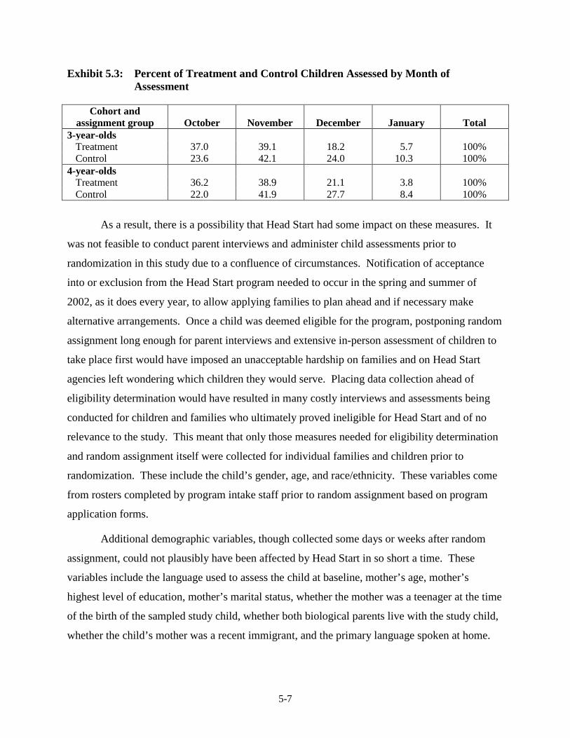
5-7
Exhibit 5.3: Percent of Treatment and Control Children Assessed by Month of Assessment
Cohort and
assignment group October November December January Total 3-year-olds
Treatment 37.0 39.1 18.2 5.7 100% Control 23.6 42.1 24.0 10.3 100%
4-year-olds Treatment 36.2 38.9 21.1 3.8 100% Control 22.0 41.9 27.7 8.4 100%
As a result, there is a possibility that Head Start had some impact on these measures. It
was not feasible to conduct parent interviews and administer child assessments prior to
randomization in this study due to a confluence of circumstances. Notification of acceptance
into or exclusion from the Head Start program needed to occur in the spring and summer of
2002, as it does every year, to allow applying families to plan ahead and if necessary make
alternative arrangements. Once a child was deemed eligible for the program, postponing random
assignment long enough for parent interviews and extensive in-person assessment of children to
take place first would have imposed an unacceptable hardship on families and on Head Start
agencies left wondering which children they would serve. Placing data collection ahead of
eligibility determination would have resulted in many costly interviews and assessments being
conducted for children and families who ultimately proved ineligible for Head Start and of no
relevance to the study. This meant that only those measures needed for eligibility determination
and random assignment itself were collected for individual families and children prior to
randomization. These include the child’s gender, age, and race/ethnicity. These variables come
from rosters completed by program intake staff prior to random assignment based on program
application forms.
Additional demographic variables, though collected some days or weeks after random
assignment, could not plausibly have been affected by Head Start in so short a time. These
variables include the language used to assess the child at baseline, mother’s age, mother’s
highest level of education, mother’s marital status, whether the mother was a teenager at the time
of the birth of the sampled study child, whether both biological parents live with the study child,
whether the child’s mother was a recent immigrant, and the primary language spoken at home.
5-8
However, the cognitive, social-emotional, health, and parenting measures used as
outcomes could have been affected by Head Start very early in children’s participation in the
program. For this reason, we do not want to include the fall 2002 versions of these variables in
the impact model in their original form. If impacts of Head Start occurred quickly in fall 2002,
inclusion of the unadjusted “pre-test” variables in the impact equation would attenuate impact
estimates. That is, Head Start would not receive full credit for the impacts it achieved in
subsequent springs because the portion of the impact achieved prior to fall 2002 data collection
would be removed by the added covariates.15
To avoid this problem, all fall 2002 “pre-test” measures of outcome variables used as
covariates are “residualized” before inclusion in the impact regressions. The “residualization”
procedure removes any systematic differences between treatment and control group levels in the
fall measures, including those potentially due to Head Start’s impact. For a given age cohort, it
subtracts the mean level of the fall measure for the entire treatment group from each individual
treatment group member’s value of that measure and does the same (using the control group
mean) for members of the control group.
16 The resulting mean-deviated variables are used as
covariates in spring impact regressions rather than the original fall variables.17
15 The measure of program impact from the regression model—the coefficient on the variable indicating
membership in the Head Start group—will include only that portion of the overall spring difference between treatment and control groups not accounted for by other variables in the model. Fall measures that are systematically higher (or lower, for factors that Head Start participation might reduce such as parental use of physical discipline) for the treatment group than for the control group, and that predict child variation in spring outcomes, will account for some of the systematically higher (or lower) spring outcomes for the Head Start group, thereby reducing the size of the coefficient measuring program impact.
Since the means
16 In practice, this procedure was accomplished by regressing the fall measure on an intercept and a dummy variable for membership in the treatment group, using the same sample and analysis weights as the spring impact regressions. (This means a given covariate is residualized multiple times, separately for each spring impact regression model; this assures that the properties sought through residualization manifest exactly each time the covariate is used in an impact regression.) The fitted equation is then used to predict a value for each individual based on her/his treatment/control group assignment, and the individual’s “residual” derived by subtracting the predicted value from the actual value. With such a simple specification for the initial regression, the model produces a predicted value equal to the treatment group mean of the variable for every individual in the treatment group, and a predicted value equal to the control group mean for every individual in the control group, resulting in a “residualized” version of the variable that is mean-deviated within each treatment/control cell.
17 Some pre-test measures used as covariates have “artificial zeros” inserted into them for children with certain language backgrounds, as explained below. In these instances, only the observations with real data values are used in the “residualization” procedure, both to compute means and in adjustments that subtract the mean. This assures that the goals of residualization are achieved for the real data values, leaving the “artificial zero” values to be accommodated by other facets of the imputation procedure.

5-9
of the “residualized” variables are 0 for both treatment and control groups, this ensures that no
part of the estimated spring impact is attenuated by their inclusion in the model.
The procedure has the drawback that the residualized fall measure will not remove
purely chance differences between treatment and control groups on the fall measure, as would
using the fall measure as a covariate directly.18 We judge this sacrifice in statistical precision to
be worth the assurance gained that the potential early impacts of Head Start will not interfere
with unbiased impact estimation in subsequent springs. To insure the precision loss is not
large, we re-ran some of the impact analyses using the original version of the fall outcome
measure without residualizing it, recognizing that this potentially biases the impact estimate but
focusing on the estimate’s standard error. Our goal was to see if the standard error (and hence
variance) of the impact estimate goes down appreciably when the fall measure retains the
information needed to offset chance differences between the treatment and control group
starting points on the pretest measure. These checks—which included re-running impacts on
child assessment outcomes from the spring of 2003 (eleven impacts for each of two age
cohorts)—showed only a trivial difference in the magnitude of the standard errors compared to
the residualized case.19
For many child assessment outcomes, the residualization was done separately by
language group within age cohort. Many of the fall tests were administered in English for both
English-speaking and Spanish-speaking children at baseline. However, performance on these
One value of including covariates in impact regressions is still realized:
variation in spring outcomes associated with the pre-existing diversity of the families and
children within the treatment group and within the control groups is still preserved in the
“residualized” covariates and continues to reduce unexplained variability in the data, thereby
improving the statistical precision of all the estimated regression coefficients, including the
impact estimates.
18 In addition to purely chance differences, differences due to differential nonresponse between the treatment and
control groups in the collection of spring outcome measures will also not be removed by using covariates that have been “residualized” in this fashion. Fortunately, it is only the effects of differential nonresponse not removed by other means—i.e., by non-response adjustments to the analysis weights used in the impact regressions (described elsewhere in the report)—that remain as an influence on the spring impact estimates when “residualized” covariates are used instead of the non-residualized covariates.
19 There was one exception among the 22 comparisons made: Woodcock-Johnson III Applied Problems, for which the residualized standard error of 2.11 was appreciably larger than the non-residualized standard error of 1.66. No other contrast was anywhere near this large.

5-10
tests depends heavily on the English-language skills of the assessed child. As a result, we expect
the assessments to measure different aspects of language and literacy potential for predominantly
English-speaking children and predominantly Spanish-speaking children, given the substantially
different capabilities with the English language the two sets of children possessed at that time.
Exhibit 5.4 provides the particular fall 2002 outcome used with each spring outcome
measure to create a “residualized” version of the fall 2002 outcome for use in the regression
model. Note that children in the Other language group were not given the PPVT, Woodcock
Johnson III Letter Word, or Woodcock Johnson III Applied Problems assessments in fall 2002,
thus it was not possible to create a residualized fall measure for them. A value of zero was
imputed for them, since zero is the mean of the residualized fall measures for the English and
Spanish groups, so they could be included in the regression modeling that produced the adjusted
impact estimates. Because the Other language group comprises only 1.5% of the sample and
5.7% of the combined Spanish/Other group, the effect of this imputation on the impact estimates
should be minor.
Exhibit 5.4: Measures of Fall 2002 “Starting Points” Used in the Regression Models, by Child and Parent Outcomes
Outcome Measure Fall 2002 Measure Used as a Covariate
Cognitive Domain Peabody Picture Vocabulary Test (PPVT) (Adapted)*
PPVT
Preschool Comprehensive Test of Phonological and Print Processing (CTOPPP) Elision Subtest *
PPVT
Letter Naming * PPVT Color Identification Color Identification Counting Bears Counting Bears McCarthy Scales of Children’s Abilities Draw-a-Design Subtest
McCarthy Scales of Children’s Abilities Draw-a-Design Subtest
Woodcock-Johnson III Letter-Word Identification * Woodcock-Johnson III: Letter-Word Identification Woodcock-Johnson III Spelling* PPVT Woodcock-Johnson III Applied Problems* Assessed Primarily in English in Fall 2002
Woodcock-Johnson III Applied Problems Assessed Primarily in Spanish in Fall 2002 Woodcock-Munoz Applied Problems
Woodcock-Johnson III Oral Comprehension* PPVT Woodcock-Johnson III Pre-Academic Skills * PPVT Woodcock-Johnson III Writing Samples* PPVT Woodcock-Johnson III Passage Comprehension* PPVT

5-11
Exhibit 5.4: Measures of Fall 2002 “Starting Points” Used in the Regression Models, by Child and Parent Outcomes (continued)
Outcome Measure Fall 2002 Measure Used as a Covariate Woodcock-Johnson III Calculation* Assessed Primarily in English in Fall 2002
Woodcock-Johnson III Applied Problems Assessed Primarily in Spanish in Fall 2002 Woodcock-Munoz Applied Problems
Woodcock-Johnson III Academic Applications* Composite
PPVT
Woodcock-Johnson III Academic Skills * PPVT Woodcock-Johnson III Basic Reading Skills* PPVT Woodcock-Johnson III Math Reasoning* Assessed Primarily in English in Fall 2002
Woodcock-Johnson III: Applied Problems Assessed Primarily in Spanish in Fall 2002 Woodcock-Munoz Applied Problems
Woodcock-Johnson III Word Attack* PPVT Woodcock-Johnson III Quantitative Concepts* Assessed Primarily in English in Fall 2002
Woodcock-Johnson III: Applied Problems Assessed Primarily in Spanish in Fall 2002 Woodcock-Munoz Applied Problems
Test de Vocabulario en Imágenes Peabody (TVIP) Assessed Primarily in Spanish in Fall 2002 Test de Vocabulario en Imágenes Peabody (TVIP)
Batería Woodcock-Muñoz Pruebas de aprovechamiento-Revisada: Identificación de letras y palabras
Assessed Primarily in Spanish in Fall 2002 Batería Woodcock-Muñoz Pruebas de aprovechamiento-Revisada: Identificación de letras y palabras
Parent (reported) Emergent Literacy Scale (PELS) Parent (reported) Emergent Literacy Scale (PELS) Social-Emotional Domain
Social Skills and Positive Approaches to Learning Social Skills and Positive Approaches to Learning Total Problem Behavior Total Problem Behavior Aggressive Behavior Aggressive Behavior Hyperactive Behavior Hyperactive Behavior Withdrawn Behavior Withdrawn Behavior Pianta Scale: Closeness None Pianta Scale: Conflict None Pianta Scale: Positive Relationship None Social Competencies Checklist Social Competencies Checklist
Parenting Practices Domain Parent used time out in the last week Parent used time out in the last week Parent spanked child in the last week Parent spanked child in the last week Parental Safety Practices Scale Parental Safety Practices Scale Family Cultural Enrichment Scale Family Cultural Enrichment Scale Parenting Style is Authoritarian Parenting Style is Authoritarian Parenting Style is Authoritative Parenting Style is Authoritative Parenting Style is Neglectful Parenting Style is Neglectful Parenting Style is Permissive Parenting Style is Permissive Parent read to child in last Parent read to child in last
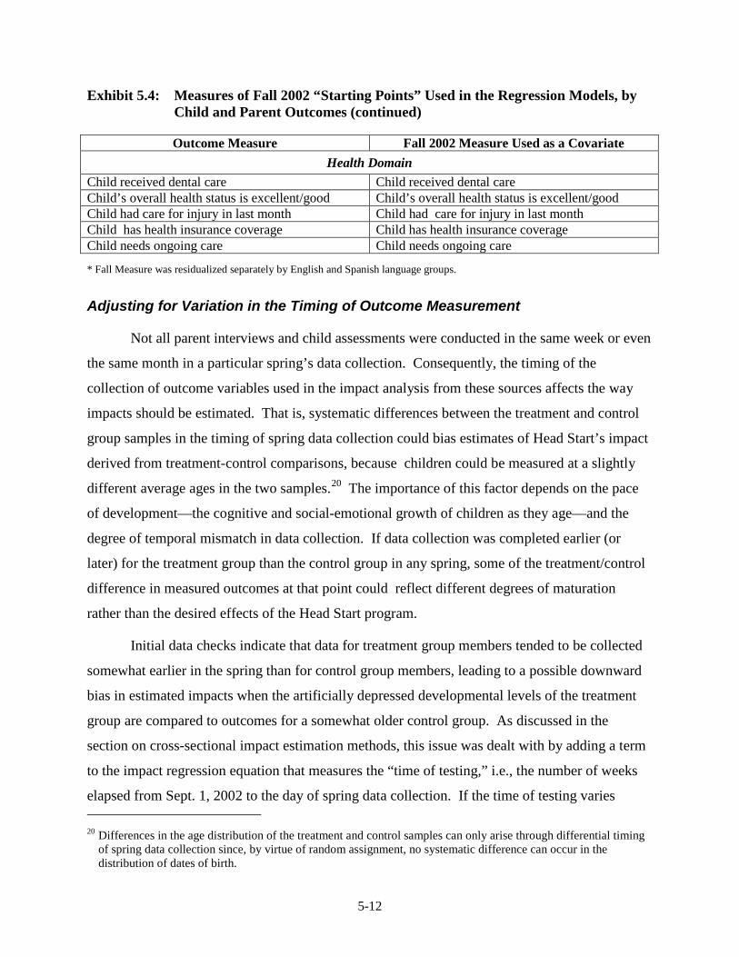
5-12
Exhibit 5.4: Measures of Fall 2002 “Starting Points” Used in the Regression Models, by Child and Parent Outcomes (continued)
Outcome Measure Fall 2002 Measure Used as a Covariate Health Domain
Child received dental care Child received dental care Child’s overall health status is excellent/good Child’s overall health status is excellent/good Child had care for injury in last month Child had care for injury in last month Child has health insurance coverage Child has health insurance coverage Child needs ongoing care Child needs ongoing care
* Fall Measure was residualized separately by English and Spanish language groups.
Adjusting for Variation in the Timing of Outcome Measurement
Not all parent interviews and child assessments were conducted in the same week or even
the same month in a particular spring’s data collection. Consequently, the timing of the
collection of outcome variables used in the impact analysis from these sources affects the way
impacts should be estimated. That is, systematic differences between the treatment and control
group samples in the timing of spring data collection could bias estimates of Head Start’s impact
derived from treatment-control comparisons, because children could be measured at a slightly
different average ages in the two samples.20
Initial data checks indicate that data for treatment group members tended to be collected
somewhat earlier in the spring than for control group members, leading to a possible downward
bias in estimated impacts when the artificially depressed developmental levels of the treatment
group are compared to outcomes for a somewhat older control group. As discussed in the
section on cross-sectional impact estimation methods, this issue was dealt with by adding a term
to the impact regression equation that measures the “time of testing,” i.e., the number of weeks
elapsed from Sept. 1, 2002 to the day of spring data collection. If the time of testing varies
The importance of this factor depends on the pace
of development—the cognitive and social-emotional growth of children as they age—and the
degree of temporal mismatch in data collection. If data collection was completed earlier (or
later) for the treatment group than the control group in any spring, some of the treatment/control
difference in measured outcomes at that point could reflect different degrees of maturation
rather than the desired effects of the Head Start program.
20 Differences in the age distribution of the treatment and control samples can only arise through differential timing
of spring data collection since, by virtue of random assignment, no systematic difference can occur in the distribution of dates of birth.

5-13
enough during the several months long spring data collection period to materially affect
outcomes on developmental measures, the coefficient of this term will differ from 0.21
Imputation for Fall 2002 Item and Instrument Nonresponse
To produce as complete a data set for impact analysis as possible, it is desirable to impute
missing responses for fall 2002 variables used as covariates or to form subgroups (for analysis of
variation in impacts).22
Hot-Deck Procedure. Fall 20002 variables missing due to item and instrument
nonresponse were imputed using hot deck imputation. Hot deck imputation is a procedure where
cases with missing values for specific variables have those “holes” in their records filled in with
values from other similar “donor” cases. Because the imputed values are actual respondents’
values, hot-deck imputation has the desirable property that imputed values are always feasible,
since they come from the actual distribution of reported values for real children. The “donor,” is
randomly selected from a pool of similar children who are matched to the “recipient,” on
characteristics which are correlated with the variable being imputed. The aim is to construct
pools or imputation classes that explain as much of the variance in the variable to be imputed as
possible, but at the same time are of adequate size so that there is some minimum number of
donors in each class so that donors are not reused too many times. The assumption is that within
each imputation class, the mechanism that leads to missing data is ignorable; that is, the missing
values are missing at random. This means that the probability that a value is missing can depend
on the values of the imputation class variables but not on the missing values themselves. If
implemented carefully, hot deck imputation can preserve the distribution of the data, so that
Imputation of baseline measures also helps to control for nonresponse
bias caused by initial nonresponse and thus to produce a more representative file for all impact
analyses. Discarding incomplete cases is inefficient, but more seriously, the complete cases may
not be representative of the target population.
21 The coefficient could also differ from 0 if time of testing is correlated with important student demographic
characteristics. However, we believe that it is more likely that age will confound results than demographic characteristics that happen to be correlated with time of testing. The model does contain the child’s age in weeks at the time of spring testing.
22 Imputation was only done for missing fall 2002 covariates. Missing data from the consecutive spring follow-ups was handled through the use of non-response weights.
5-14
estimates of distributional characteristics such as percentiles, variability, and correlation will not
be distorted.
The variables used to form imputation classes or cells were identified from chi-square
tests of association and bivariate correlation coefficients. In some cases they were also
determined by skip patterns in the parent questionnaire and other requirements of logical
consistency between questionnaire items. The imputation cells were created as the Cartesian
product of these variables. A donor was allowed to be used up to three times. When no more
donors were available in an imputation class, adjacent cells were collapsed to expand the
availability of potential donors. The order of collapsing was specified so that levels of the least
correlated cell variable were collapsed first, followed by the second least correlated variable, etc.
until a donor was found. Imputed values have been flagged so that an analyst has the option of
not using the imputed data, such as when analyzing the effects of the imputed data on the results.
Variables That Were Imputed. Missing values for demographic variables, child health
outcomes, social-emotional and scale variables were imputed for the entire sample; missing
values for test score variables were imputed for all sample members of the language group that
should have completed the particular assessment (see previous discussion of outcome measures).
The variables that underwent imputation and their item nonresponse rates are given in
Exhibit 5.5 for variables used in the analysis. The item nonresponse rate was calculated as the
number of children for whom the item was missing (and hence imputed) divided by the total
number of children eligible for the item. For any given spring data collection, item nonresponse
rates will be lower than those in Exhibit 5.5 after conditioning on overall response status for the
child assessment, since many of the item nonrespondents are also survey nonrespondents for the
spring assessment. Among spring 2003 child assessment respondents, the nonresponse rates for
demographic variables ranged from < 1% to 16%. Child health outcomes, scores and scale
variables had missing rates ranging from 9% to 12%.
Use of Correlation and Missing Data Patterns. The multivariate relationships between
items were taken into account in the imputation to maintain consistency of the data and attempt
to preserve correlations among variables. Continuous correlated items such as assessment scores
or social-emotional scales were usually imputed from a single donor child. The donor was
randomly selected from within a donor pool of children matched by treatment/control group
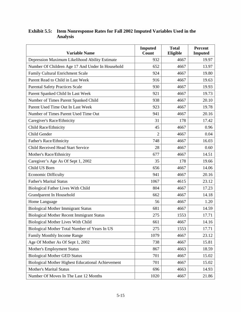
5-15
Exhibit 5.5: Item Nonresponse Rates for Fall 2002 Imputed Variables Used in the Analysis
Variable Name Imputed Count
Total Eligible
Percent Imputed
Depression Maximum Likelihood Ability Estimate 932 4667 19.97 Number Of Children Age 17 And Under In Household 652 4667 13.97 Family Cultural Enrichment Scale 924 4667 19.80 Parent Read to Child in Last Week 916 4667 19.63 Parental Safety Practices Scale 930 4667 19.93 Parent Spanked Child In Last Week 921 4667 19.73 Number of Times Parent Spanked Child 938 4667 20.10 Parent Used Time Out In Last Week 923 4667 19.78 Number of Times Parent Used Time Out 941 4667 20.16 Caregiver's Race/Ethnicity 31 178 17.42 Child Race/Ethnicity 45 4667 0.96 Child Gender 2 4667 0.04 Father's Race/Ethnicity 748 4667 16.03 Child Received Head Start Service 28 4667 0.60 Mother's Race/Ethnicity 677 4667 14.51 Caregiver’s Age As Of Sept 1, 2002 35 178 19.66 Child US Born 656 4667 14.06 Economic Difficulty 941 4667 20.16 Father's Marital Status 1067 4615 23.12 Biological Father Lives With Child 804 4667 17.23 Grandparent In Household 662 4667 14.18 Home Language 56 4667 1.20 Biological Mother Immigrant Status 681 4667 14.59 Biological Mother Recent Immigrant Status 275 1553 17.71 Biological Mother Lives With Child 661 4667 14.16 Biological Mother Total Number of Years In US 275 1553 17.71 Family Monthly Income Range 1079 4667 23.12 Age Of Mother As Of Sept 1, 2002 738 4667 15.81 Mother's Employment Status 867 4663 18.59 Biological Mother GED Status 701 4667 15.02 Biological Mother Highest Educational Achievement 701 4667 15.02 Mother's Marital Status 696 4663 14.93 Number Of Moves In The Last 12 Months 1020 4667 21.86
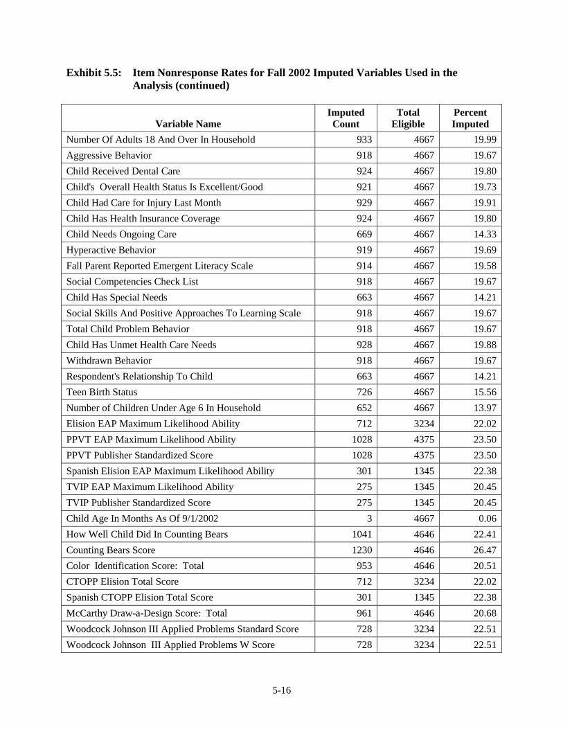
5-16
Exhibit 5.5: Item Nonresponse Rates for Fall 2002 Imputed Variables Used in the Analysis (continued)
Variable Name Imputed Count
Total Eligible
Percent Imputed
Number Of Adults 18 And Over In Household 933 4667 19.99 Aggressive Behavior 918 4667 19.67 Child Received Dental Care 924 4667 19.80 Child's Overall Health Status Is Excellent/Good 921 4667 19.73 Child Had Care for Injury Last Month 929 4667 19.91 Child Has Health Insurance Coverage 924 4667 19.80 Child Needs Ongoing Care 669 4667 14.33 Hyperactive Behavior 919 4667 19.69 Fall Parent Reported Emergent Literacy Scale 914 4667 19.58 Social Competencies Check List 918 4667 19.67 Child Has Special Needs 663 4667 14.21 Social Skills And Positive Approaches To Learning Scale 918 4667 19.67 Total Child Problem Behavior 918 4667 19.67 Child Has Unmet Health Care Needs 928 4667 19.88 Withdrawn Behavior 918 4667 19.67 Respondent's Relationship To Child 663 4667 14.21 Teen Birth Status 726 4667 15.56 Number of Children Under Age 6 In Household 652 4667 13.97 Elision EAP Maximum Likelihood Ability 712 3234 22.02 PPVT EAP Maximum Likelihood Ability 1028 4375 23.50 PPVT Publisher Standardized Score 1028 4375 23.50 Spanish Elision EAP Maximum Likelihood Ability 301 1345 22.38 TVIP EAP Maximum Likelihood Ability 275 1345 20.45 TVIP Publisher Standardized Score 275 1345 20.45 Child Age In Months As Of 9/1/2002 3 4667 0.06 How Well Child Did In Counting Bears 1041 4646 22.41 Counting Bears Score 1230 4646 26.47 Color Identification Score: Total 953 4646 20.51 CTOPP Elision Total Score 712 3234 22.02 Spanish CTOPP Elision Total Score 301 1345 22.38 McCarthy Draw-a-Design Score: Total 961 4646 20.68 Woodcock Johnson III Applied Problems Standard Score 728 3234 22.51 Woodcock Johnson III Applied Problems W Score 728 3234 22.51
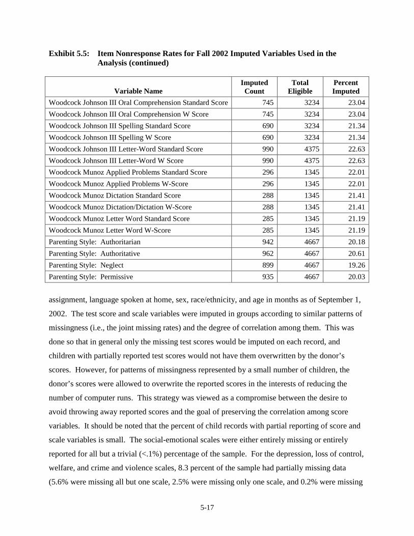
5-17
Exhibit 5.5: Item Nonresponse Rates for Fall 2002 Imputed Variables Used in the Analysis (continued)
Variable Name Imputed Count
Total Eligible
Percent Imputed
Woodcock Johnson III Oral Comprehension Standard Score 745 3234 23.04 Woodcock Johnson III Oral Comprehension W Score 745 3234 23.04 Woodcock Johnson III Spelling Standard Score 690 3234 21.34 Woodcock Johnson III Spelling W Score 690 3234 21.34 Woodcock Johnson III Letter-Word Standard Score 990 4375 22.63 Woodcock Johnson III Letter-Word W Score 990 4375 22.63 Woodcock Munoz Applied Problems Standard Score 296 1345 22.01 Woodcock Munoz Applied Problems W-Score 296 1345 22.01 Woodcock Munoz Dictation Standard Score 288 1345 21.41 Woodcock Munoz Dictation/Dictation W-Score 288 1345 21.41 Woodcock Munoz Letter Word Standard Score 285 1345 21.19 Woodcock Munoz Letter Word W-Score 285 1345 21.19 Parenting Style: Authoritarian 942 4667 20.18 Parenting Style: Authoritative 962 4667 20.61 Parenting Style: Neglect 899 4667 19.26 Parenting Style: Permissive 935 4667 20.03
assignment, language spoken at home, sex, race/ethnicity, and age in months as of September 1,
2002. The test score and scale variables were imputed in groups according to similar patterns of
missingness (i.e., the joint missing rates) and the degree of correlation among them. This was
done so that in general only the missing test scores would be imputed on each record, and
children with partially reported test scores would not have them overwritten by the donor’s
scores. However, for patterns of missingness represented by a small number of children, the
donor’s scores were allowed to overwrite the reported scores in the interests of reducing the
number of computer runs. This strategy was viewed as a compromise between the desire to
avoid throwing away reported scores and the goal of preserving the correlation among score
variables. It should be noted that the percent of child records with partial reporting of score and
scale variables is small. The social-emotional scales were either entirely missing or entirely
reported for all but a trivial (<.1%) percentage of the sample. For the depression, loss of control,
welfare, and crime and violence scales, 8.3 percent of the sample had partially missing data
(5.6% were missing all but one scale, 2.5% were missing only one scale, and 0.2% were missing

5-18
some other combination). For the continuous test score variables, less than 5 percent of the
sample had partial reporting of scores; most were either missing all scores or none.
The order in which items are imputed is also important in preserving the correlation
structure in the data, because some imputed items can be used to form imputation cells in the
subsequent imputation of related items. Attention to the ordering of imputation was important,
for example, in the imputation of categorical assessment scores (e.g., so that the first score that
was imputed could be used to create imputation cells for the next test score. It was also used
throughout in the imputation of correlated demographic and household variables. Similarly, for
items associated with a skip pattern in the parent questionnaire, the item that leads into the skip
pattern was imputed first and the subsequent items were imputed depending on the value of the
skip indicator. In addition, the demographic variables (i.e., were imputed first, and were then
subsequently used to impute parenting practice, household income, child health outcomes,
assessment scores and scale variables. Items with the least amount of nonresponse within a
group of related categorical variables were imputed first, and then used in the imputation of
items with larger amounts of missing data.
Role of Geography. In general, donors were randomly selected from within the same
Head Start program within a cell when possible, collapsing with an adjacent program in the cell
when necessary. Programs were sorted within a cell by primary sampling unit (PSU) within
Census region, so adjacent programs tended to be from the same county or a nearby county.
When there were a large number of imputation cells, the donor search often was broadened to the
geographic PSU within a cell, and sometimes PSUs within a region were also collapsed. Some
items such as fall scores required a closer match on demographic variables than geography or
Head Start program in order to find a similar donor pool, and no attempt to stay within the PSU
or program was made for these. For example, donors for fall scores were matched by home
language, gender, race and age as of Sept 1, 2002 in months within the Head Start/non-Head
Start groups. Geography was also ignored for certain items requiring a very close match to the
donor on other questionnaire items for logical consistency.
Imputation Results. The distribution of each imputed variable was compared before
and after imputation to check that the imputation procedures had not appreciably changed the
distribution of the underlying variable. Correlation matrices were also examined to check that
5-19
bivariate correlations among scores and scales were not attenuated. Finally, crosstabs between
categorical variables involved in skip patterns and those requiring logical consistency were
checked to make sure that inconsistencies had not been introduced.
Sample Sizes, Target Populations, and Analysis Weights
The unit of analysis for all impact analyses is the child. This is true irrespective of the
outcome measure or data source considered; even outcomes reported by parents and caregivers
(the majority) are weighted and analyzed according to the children they describe. This makes all
impact findings representative of all newly entering Head Start children in the nation in 2002.
Two separate samples were selected, one for children entering Head Start one year before
their anticipated entry into kindergarten – referred to as the 4-year-old cohort – and one for
children entering Head Start two years prior to their expected kindergarten entry – referred to as
the 3-year-old cohort. All analyses are conducted separately for the two cohorts rather than as a
pooled single analysis sample. This decision to conduct separate age-cohort analyses reflects the
fact that children are at very different developmental stages at these two ages, and that the Head
Start treatment differs markedly by age, not the least because of the smaller class sizes required
for younger children and other programmatic factors. This division also corresponds to the
structure of the original random assignment, which was done separately for the two age cohorts
to run separate experiments that used two different definitions of the control group experience:
no Head Start participation for the 4-year-old cohort, versus a one-year postponement of Head
Start participation for the 3-year-old cohort (for which the control group was allowed to enter
Head Start in the second year). Finally, the demographic composition of the group of children
who enter Head Start at age three is very different from the group who enter at age four.
Conducting the analyses separately allows the statistical models to make the appropriate
adjustments for baseline differences in a way that best corresponds to these differences.
As described in Chapter 2, some children could not be tested in English at the time of the
baseline assessments in fall 2002. These children were administered two Spanish language tests
in both fall 2002 and spring 2003, i.e., the TVIP (adapted) and the Woodcock-Muñoz Letter-
Word Identification Test. Separate impact estimates were developed for this group of children
on these Spanish language assessments. Like all subgroups defined by characteristics
independent of the intervention and not affected by random assignment, these language-based

5-20
subsamples are, but for chance,23
All of the children in the study sample from Puerto Rico began with Spanish-language
assessments and continued exclusively in that language throughout the study period (since
transition to bilingualism through English acquisition does not commonly take place until a later
grade). Because cognitive measures administered in different languages are not directly
comparable, Puerto Rican children are analyzed separately from their “mainland” counterparts in
Appendix F in the Final Report of the Head Start Impact Study.
well-matched in terms of children in the Head Start and control
groups. Hence, they are fully suited to valid experimental examination in their own right. Thus,
the separate language-of-assessment analyses provide equally unbiased measures of Head Start’s
impact for these subpopulations, as does the study as a whole for the full population.
The weighting strategy, described in more detail in Chapter 2, was chosen to maximize
the data available at each analysis point by including every completed child assessment and
parent interview from each wave of spring data collection. Observations were compiled
separately for child assessments, parent interviews, and teacher reports and information included
from one of these sources even when one or more of the other sources may have been missing.
For this reason, and also due to item nonresponse for specific questions in completed
questionnaires, sample sizes are not identical for all analyses, i.e., different outcome variables
involve slightly differing numbers of observations. The comparability of the Head Start and
control group samples established at random assignment is maintained to the greatest extent
possible in each instance by adjusting the initial sampling weights to offset observable baseline
differences between respondents and non-respondents.
Analysis weights were established separately for the child assessments and the parent
interview each spring, for use in the annual cross-sectional analysis of Head Start impacts in each
follow-up year. These weights are based on the probability of selection into the study sample,
including all stages of sampling, and were adjusted each year to compensate for nonresponse by
adjusting the weight for responding children with similar individual and family background
characteristics on variables measured for all randomly assigned children in fall 2002. The
weights also include an adjustment to the program and center weights for the exclusion of 23 In addition to chance, the comparability of the treatment and control group samples for different language groups
depends on the success of the nonresponse weight adjustments made to the overall sample to deal with possible differential nonresponse in spring data collection, discussed in Chapter 2.

5-21
grantees and centers in which the number of applicants did not exceed the number of funded
federal Head Start slots. The weighted data, therefore, represent the same universe for all spring
outcomes each analysis year; namely, the national population of 3- and 4-year-olds who entered
Head Start for the first time in fall 2002.
A separate weight was also created for analysis of Teacher Survey/Teacher Child Rating
outcomes from spring 2004 to spring 2006. The Teacher Survey and Teacher Child Rating were
administered to teachers of sampled children in pre-K programs in centers (both Head Start and
non Head Start programs), or who were in kindergarten or first grade. Separate weights were
also created for analysis of the Director Interview data, and for analysis of classroom
observations collected at children’s out of home child care placements.
A separate analysis weight was also created for longitudinal analysis of children who
had two or more spring data collection points between Fall 2002 and Spring 2006 (see Chapter
2). The longitudinal weight permits these children to represent the population of children who
applied for their Head Start year in fall 2002. It was created by adjusting the child base weight
for children, who did not have at least two data points, then poststratifying and trimming the
weight in the same manner as the cross-sectional weights. The weight was used in the fitting of
growth curves using multilevel modeling software by partitioning it into the center weight and
within-center child weight, to correspond to the center and child levels in the three-level model
(see section on repeated measures analysis). The level one child weight was then scaled using
method two as described in Pfeffermann (1998), so that the scaled weights sum to the nominal
sample size of children within center.
Profiles of the sampled Head Start and control group children with respect to
demographic and family characteristics are provided in Chapter 2 separately by year and age
cohort. Each exhibit compares the unweighted distribution of the sampled respondents at each
spring data collection (spring 2003 to spring 2006) with the weighted distributions, using both
the child base weight and the final child weight. The final weight includes a nonresponse
adjustment for both age cohorts, and a poststratification adjustment to the race/ethnicity
distribution of the Head Start National Reporting System (HSNRS) for the 4-year-old cohort in
the sample (the HSNRS does not provide data for 3-year-olds), since the HSNRS is a census of
4-year-old Head Start enrollees. The poststratification adjustment has the effect of

5-22
downweighting the weights of Hispanic children and increasing the weights of Black children
to more closely match the distribution of the HSNRS. The effect of the poststratification can be
seen in the Child Race/Ethnicity exhibit when comparing the “Base Weights” and “Final
Weights” columns. The exhibits also show that the composition of the sampled respondents
has remained stable over time, whether unweighted or weighted.
Exhibit 5.6 shows the number of respondents for the Head Start and control groups by
age cohort and year, separately for the child assessments, parent interview, and teacher
survey/teacher child rating. Overlap among respondents for the three different data collection
instruments is considerable for both age cohorts, i.e., sample sizes track closely between the
three different data sources.24
Exhibit 5.6: Number of Respondents by Wave and Age Cohort Fall 2002 2003 2004 2005 2006
Instrument Age
3 Age
4 Age
3 Age
4 Age
3 Age
4 Age
3 Age
4 Age
3 Age
4 Child Assessment
Head Start 1310 1050 1357 1084 1322 1009 1251 1003 1281 NA Non-Head Start 746 617 808 649 816 615 769 616 742 NA
Parent Interview Head Start 1387 1102 1336 1068 1320 1022 1295 1032 1274 NA
Non-Head Start 847 679 821 662 806 627 798 640 772 NA Teacher Survey and Child Rating
Head Start NA NA NA NA NA 659 1032 779 1028 NA Non-Head Start NA NA NA NA NA 401 632 483 643 NA
NA indicates not applicable.
Annual Cross-Sectional Impact Estimation Methods–Main Impacts
The impact of Head Start is assessed using (1) simple treatment-control differences in
average child and parent outcomes and (2) differences in average outcomes adjusted for the set
of baseline covariates discussed above. Both methods are discussed below.
24 There are only two ways to move closer to a single, totally uniform sample for each age cohort so that impacts on
all outcomes would derive from exactly the same set of cases: impute missing outcomes (and entirely missing data collection instruments) for cases with available data for some but not all outcome measures in all years, or choose not to use data that are available by excluding from all analyses observations with less than universal data. We do neither of these: the latter would waste information while cutting sample sizes unnecessarily while the former would require assumptions too closely intertwined with the program impacts the study intends to measure.
5-23
Differences in Average Outcomes
The Head Start Impact Study, like other evaluations that use random assignment to
allocate slots to program participants, provides a framework for attributing child outcomes to the
effects of the program, rather than to other factors that may influence child development. Unlike
pre-test/post-test analyses and other comparison group approaches, this framework makes
accurate impact measurement possible without considering any individual child’s starting point.
If enough individuals are randomized to the Head Start and control groups, and if all randomized
individuals are included in the follow-up analysis, important differences in later outcomes are
more likely to result from the intervention rather than other factors. Actual measurement, and
adjustment for possible chance differences in starting points, is not essential under this design
(although it can be useful for certain reasons, as discussed below).
The simplicity of the basic treatment/control comparison of spring outcomes, without
recourse to other data, provides a powerful motivation for evaluating program impacts in this
way. The transparency of the methodology, and its lack of dependence on sometimes complex
statistical methods, makes these “difference-in-means” results good candidates as initial
measures of Head Start’s impact. The most basic version of this analysis contrasts the average
outcome level for the treatment group with the average outcome level for the control group using
unweighted data. However, the unweighted estimates can be biased because they do not take
into account the differential probabilities of selection of children into the sample. The child
weights account for the sampling of PSUs, grantee/delegate agencies, centers, and children
within centers so that the study sample can be used to represent the national Head Start
population.
These weighted difference-in-means impact estimates are reported as the basic estimates
in this report. Statistical tests determine which of the measured outcome differences between
treatment and control group children can be considered real impacts rather than simply due to
sampling error. For continuous outcome variables (e.g., PPVT III scale score), the tests are
based on the linear regression model that replicates the difference-in-means calculation by
expressing the spring outcome measure for child i as the sum of an intercept term and a shift in
the intercept produced by a dummy variable for inclusion in the Head Start treatment group:
;TY iii ε+β+α=

5-24
where Yi is the outcome measure and Ti is a 0-1 variable indicating whether the child was
randomly assigned to the treatment group (Ti = 1) or the control group (Ti = 0). When derived
using weighted least-squares regression, the estimated coefficients from this model, α̂ β̂
have the following equivalence to calculated measures from the difference-in-mean appro
and
ach:
ct
c
yyˆyˆ
−=β=α
where ty is the weighted mean of Y for the treatment (Head Start) sample and cy is the weighted
mean of Y for the control (non-Head Start) sample. By either formulation, β̂ gives an unbiased
estimate of the impact of access to Head Start, since no systematic differences should exist
between the treatment and control samples (assuming complete follow-up data on Y), given
children were randomly assigned to each group within Head Start centers. When divided by its
standard error, β̂ in large samples for continuous outcomes follows the Students t-distribution
with 51 degrees of freedom under the null hypothesis that true impact, β is 0, where 51 is the
total number of degrees of freedom associated with the jackknife estimate of the variance of β̂ .
An unbiased standard error for β̂ , reflective of how the sample was drawn and weighted is
obtained using replicates and weights described in Chapter 2.
Calculated p-values are also given for each estimated β̂ , assuming a two-tailed t-test of
the null hypothesis of no Head Start impact (i.e., H0:β =0).25
The 95-percent confidence interval for the true impact,
This indicates the probability of
obtaining an impact estimate of at least the magnitude observed when the true impact is 0, and
allows readers to perform tests of statistical significance at different alpha levels (e.g., .10, .05 or
.01) by comparing the p-value to alpha.
,YY CT − is also reported:
( ct yy − ) – t.975,dfSE( ct yy − ) < ct YY − < ( ct yy − ) + t.975,dfSE( ct yy − ),
The interpretation of the confidence interval is if all possible samples were drawn, then
95 of the confidence intervals constructed from these samples would contain the true impact.
Note, it does not mean that the true impact has a 95 percent chance of being between the lower 25 A two-tailed test allows for the possibility of program effects in either direction, up or down.

5-25
and upper limits for a given sample. Detailed tables providing confidence intervals will be
provided on the Administration for Children and Families, Office of Planning Research and
Evaluation website: http://www.acf.hhs.gov/program/opre/hs/impact_study index.html.
For binary outcome variables (e.g., use of dental care), logistic regression is used to do
equivalent computations. Categorical outcome variables with more than two categories (e.g.,
Number of Times Read To) were collapsed into two categories. Here, the model specification is
non-linear to accommodate the Bernoulli distribution of Y, which must always take on a value of
0 or 1, and to ensure that Pr(Y=1) is always between 0 and 1. The logistic model specifies the
probability that Y equals 1 (conditional on T) for the ith child as
Pi = Pr (Yi =1) = )T exp(1
)T exp(
i
i
βαβα++
+,
where Ti is the treatment group/control group indicator defined above. The coefficients α and β
are estimated using the logit transformation to obtain a model which is linear in the parameters
ii
i TP1
Pln βα +=
−
The predicted probability that Y=1 for the ith child is
)ˆˆexp(1)ˆˆexp(ˆ
i
ii T
T P
βαβα++
+= .
The predicted marginal, tP̂ , for the treatment group is obtained by taking the weighted average of
the iP̂ ‘s evaluated at Ti = 1 for every child in the sample, using the cross-sectional child weight.
The predicted marginal represents the average predicted outcome if all children had been in the
treatment group (Korn and Graubard, 1999). Similarly a predi
iP̂
cted marginal for the control
group, cP̂ , is obtained by taking the weighted average of the ‘s evaluated at Ti = 0 for every
child in the sample. The impact of Head Start is estimated as the difference ct PP ˆˆ − . Calculated
p-values are also given, assuming a two-sided t-test of the null hypothesis of no Head Start
impact (i.e., H0: Pt - Pc = 0).

5-26
Differences in Adjusted Average Outcomes
To add the explanatory power of child and family background factors to the analysis, the
regression models used to obtain difference-in-means estimates are expanded to express
outcomes (or, in the case of logistic models, the probability of a particular outcome) as a function
of assignment to the treatment group, and the set of covariates discussed in earlier in this Chapter
.26
Letting Ti represent for child i the treatment indicator, Xi that child’s vector of
demographic covariates and time of testing variable, and Ri the “residualized” fall 2002 measure,
the impact model becomes:
Note that the addition of these covariates does not decrease the sample size, since missing
values for the covariates and fall measures used in the model were imputed.
'i i i i iY T X R eα β γ δ= + + + +
for continuous outcome variables
Pi = )R XγT exp(1
)R XγT exp(
ii'
i
i'
i
δβαδβα++++
+++
for dichotomous (0/1) outcome variables. The coefficients in the continuous outcome model are
estimated using weighted least-squares regression, and in the binary outcome model using the
logit transformation to obtain a model which is linear in the parameters:
ii'
ii
i R XγT P1
Pln δβα +++=
−
For continuous outcomes, is the estimate of Head Start’s impact. Calculated p-values
are also given for each estimated β̂ , assuming a two-tailed t-test of the null hypothesis of no
Head Start impact (i.e., H0:β =0).27
26 Outcomes derived from the teacher child rating form do not have a corresponding pretest measure so this term is
dropped from these impact analyses.
This indicates the probability of obtaining an impact
estimate of at least the magnitude observed when the true impact is 0, and allows readers to
perform tests of statistical significance at different alpha levels (e.g., .10, 05 or .01) by
comparing the p-value to alpha
27A two-tailed test allows for the possibility of program effects in either direction, up or down.
β̂

5-27
For binary outcomes, the impact estimate is obtained by first calculating the predicted
probability that Y=1 for the ith child,
)ˆˆˆˆexp(1)ˆˆˆˆexp(ˆ
iii
iiii R T
R T P
δβαδβα++++
+++=
XγXγ
'
'
.
The predicted marginal, tP̂ , for the treatment group is then obtained by taking the
weighted average of the iP̂ ‘s evaluated at Ti = 1 for every child in the sample, where the
covariates and “residualized” fall score are set to the child’s individual values and the child
weight is used (Korn and Graubard, 1999). Similarly a predicted marginal, cP̂ , for the control
group is obtained by taking the weighted average of the iP̂ ‘s evaluated at Ti = 0 for every child in
the sample. The impact of Head Start is estimated as the difference ct PP ˆˆ − . Calculated p-values
are also given—i.e., the probability of obtaining an observed impact estimate of at least the size
seen when the true impact is 0—so that different significance levels (different alpha values; e.g.,
.10, .05 or .01) can be applied by the reader.
All estimation, model fitting and hypothesis testing was done with the SUDAAN
(Research Triangle Institute, 2005) software package using the full-sample and jackknife
replicate weights, to take into account the complex sample design (i.e., stratification, clustering)
and weighting in the estimation of standard errors for the regression coefficients and the impact
estimates.
When the “residualization” of the fall 2002 child assessment was done separately by
assessment language group, the residualized fall measure Ri was entered into the model as a two-
way interaction with the language group indicator, Li (where Li = 1 for children initially assessed
primarily in English and Li = 0 for children initially assessed primarily in Spanish or some other
language). This allows the pre-test assessment score to play a distinct explanatory role in
predicting spring outcomes for initially English-speaking children and initially non-English-
speaking children. Specifically, three variables replace the variable Ri in the equations above,
each with its own coefficient:28
28 A more compact representation of the two-way interaction substitutes the expression R*L into the impact
equations in place of R. All of variables listed here, each with its own coefficient, are subsumed in this notation.

5-28
The language group indicator variable, Li (= 1 if child i was initially assessed primarily in English in fall 2002, = 0 for all other children);
The residualized pre-test measure (Ri) interacted with the language group indicator variable, creating Ri Li; and
The residualized pre-test measure interacted with the reverse of the language group indicator variable, 1-Li (= 0 if child i was initially assessed primarily in English in fall 2002, = 1 for all other children), creating Ri (1-Li).
This specification in effect creates two distinct pre-test measures to use as independent
predictors, RiLi for initially English-speaking children and Ri (1-Li) for children who initially
speak little or no English. It assigns an artificial value of 0 to those variables for children not in
the particular language group involved: a zero value for RiLi for children originally assessed
predominantly in English, and a zero value for Ri (1-Li) for children originally assessed
predominantly in Spanish and other languages. Were just these two pre-test variables added to
the model with no further adjustments, the “artificial zeroes” they contain would distort estimates
of the coefficients in the model, since they do not have the same meaning as “true” zeros. The
addition of the language indicator variable Li neutralizes this potential distortion and leaves all
the other estimates in the model unchanged, including, crucially, the estimate of Head Start’s

5-29
impact, β. At the same time, it accounts for more of the variation in outcomes within each of the
language-defined subgroups.29
Standards of Evidence for Interpreting Multiple Impact Estimates
Standard statistical methods for determining if impacts of Head Start differ from zero,
such as those described above with alpha = 0.10, limit the likelihood of a “false positive” result
from any one test to 10 percent. That is, the chances of rejecting the null hypothesis of zero
impact when in fact it is true is 1 in 10 with alpha = 0.10 as above, or 1 in 20 when alpha is set
more conservatively to 0.05. However, the probability of incorrectly concluding that a non-reo
impact has occurred goes up dramatically when many different outcomes are examined, as in the
current study. For example, 10 hypothesis tests—each with a 0.05 probability of producing a
false positive result if Head Start has not impact—have a 0.40 probability of generating at least
one false positive if in fact the program has no impact on any outcome. In this instance, one
must avoid generating a false positive with every test run—a 0.95 probability in every case when
Head Start has no impact on any of the outcomes. This makes the probability of avoiding all
29 To see how the addition of Li protects against distortions of the regression coefficients and increases the
explanatory power of the model, consider how the linear model used (linear in the log-odds ratio, for categorical outcomes) seeks to accommodate 0 values if Li is left out. In that case, the relationship of the artificial zero values to the outcome variable Yi would have to be reflected by the same estimated coefficient as the influence of other real values of these variables for children actually in the language group of interest, creating inaccuracies in how the model accounts for pre-test scores in both language groups. If those scores are correlated with other variables in the model—including Ti, the indicator of assignment to the treatment or control group—this opens the door to distortions in how the model represents those factors as well. It also seriously diminishes the amount of predictive information the model can extract from the pre-test measures—the very purpose for including pre-test measures in the regressions in the first place—by muting the contribution the real values can make to explaining outcomes as their mode of transmission is confounded by the artificial zeros. This threat is removed by adding the language indicator variable, L, which gives the model the ability to explain anything distinctive about the spring outcome levels of the artificial 0 cases through an intercept shift, away from the main regression line determined by real values of Ri, without disturbing anything else the model estimates. The coefficient on Li supplies the shift amount; if the outcome variable Yi for the English-speaking children is distinctive at all (as we would expect), its tendency to be above or below the point at which the model fit to the non-English-speaking children’s data hits the vertical axis will be fully reflected in this coefficient. Note that with a constant term already in the model it is neither possible nor necessary to include a second indicator variable coded the reverse of the first (i.e., equal to 1 for the Spanish-speaking children and 0 for everyone else). The neutralizing of artificial 0s for this complementary set of individuals is accomplished by the same indicator variable, since—by defining simultaneously both the English-speaking and non-English-speaking children—its coefficient can reflect the net of the intercept shifts needed to neutralize artificial 0s for both of the pre-test variables. Also, the indicator variable Li does not distinguish the small number of children whose language background was neither English nor Spanish at baseline from initially Spanish-speaking children; it is 0 for both groups. The cognitive assessments were not administered to non-English, non-Spanish children at baseline. To approximate what scores might have been recorded for those children had they been administered in English the mean value of Ri for Spanish-speaking children is inserted for each of these children.

5-30
false positives (0.95)10 = 0.60, resulting in a 0.40 probability of generating one or more false
positives. The risk of one or more false positives is 0.65 when 10 tests are run using alpha =
0.10 (since (.90)10 = 0.35).
To limit the occurrence of false positives, the set of outcome measures used for a given
age cohort in a given spring are grouped into five “families”: two families comprised of
cognitive outcomes taken from direct child assessments and teacher-school performance
measures, plus three families consisting of all outcomes in the social-emotional, health, and
parenting domains respectively. A procedure due to Benjamini and Hochberg (1995) is then
used to limit the “false discovery rate” in each family of outcomes to no more than 10 percent.
This procedure ensures that at most 10 percent of the impact estimates declared statistically
significantly different from zero is a false positive—i.e., an instance in which Head Start in fact
had no impact.
To implement this procedure, the original p-values for the individual impact estimates are
ranked from 1 to m, where m is the total number of impacts estimated for the family. Each
p-value is then compared to a calculated value equal to the value of its rank position in the
ordering (e.g., rank position “m” for the largest p-value, rank position “m-1” for the next largest,
and so on) multiplied by 0.05 and divided by m. A particular estimate is declared statistically
significant in this multiple comparison test only if it is smaller than this calculated value.
In the subgroup analysis described below, five families of tests were created for each
subgroup, using the same division of outcome measures described above, and the Benjamini-
Hochberg procedure applied to each family and each subgroup. Additional families were created
for estimated differences in impacts between subgroups; again, five families were created for
each pairwise contrast between subgroups. Hence, for example, when race/ethnicity is used to
form subgroups, a total of 30 families of tests are created:

5-31
Cognitive Outcomes Other Outcomes
Direct Child Assessments
School Teacher
Performance Social-
Emotional Health Parenting Impact on
White children √ √ √ √ √ Black children √ √ √ √ √ Hispanic children √ √ √ √ √
Difference in Impact Between
White & Black √ √ √ √ √ White & Hispanic √ √ √ √ √ Black & Hispanic √ √ √ √ √
For both main effects and subgroup impacts, the presentation of findings in the main
report tables follows a consistent protocol—or standard of evidence—for which estimated
impacts of Head Start are highlighted in exhibits and discussed in the text:
What we have in the chapter text is:
Strong Evidence of a Non -zero Impact: the estimated impact for a particular outcome is statistically significant at the typical level (p≤0.05), and this result holds up under the test for multiple comparisons.
Moderate Evidence of a Non-zero Impact: the estimated impact for a particular outcome is statistically significant at the typical level (p≤0.05), but this result does not hold up under the test for multiple comparisons.
Suggestive Evidence of a Non-zero Impact: the estimated impact for a particular outcome is statistically significant under a relaxed standard (p≤0.10), and this result may or may not hold up under the test for multiple comparisons.
Adjusting for the Variation in the Timing of Outcome Measurement
As discussed in an earlier section of this Chapter, not all parent interviews and child
assessments were conducted in the same week or even the same month in a particular spring’s
data collection. To deal with the possible introduction of bias in the annual cross-sectional
analyses, a term is included in the vector of covariates, Xi, in the impact equation to measure the
number of weeks elapsed from September 1, 2002 (the date for the calculation of every child’s
age) to the day of spring testing.

5-32
If this variable varies enough during a several months long spring data collection period
to materially affect outcomes of 3- to 6-year-old children on age-related developmental
measures, its coefficient will differ from 0. Further, if age at data collection has a different
distribution for the treatment group than the control group, the variable will correlate with the
treatment group dummy variable and the impact estimate β̂ will shift somewhat. Any change
in this coefficient will represent a neutralization of the developmental difference between
treatment and control group children at the time the outcome was measured and thus constitute
an improvement in the measurement of the effect Head Start participation per se had on
treatment group members at that time.30
Calculating Effect Sizes
Impact estimates in their initial units are converted into effect sizes by dividing by the
standard deviation of the outcome in the control group.31 This provides a “yardstick” for
gauging the quantitative importance of the estimated impact in relation to the natural variation of
the child or family outcome Head Start is seeking to affect. Effect sizes tell us how much
improvements produced by Head Start move children upward in the distribution of outcomes that
would have prevailed had no Head Start intervention been available. The square root of the
population variance of the outcome measure for the control group—the standard deviation of that
measure—provides the best measure of that distribution and the conventional standard for this
assessment.32
30 The coefficient could also differ from 0 because of selection patterns in the types of children whose data get
collected earlier or later in the spring, since it will pick up the influence of any factors that correlate with the timing of spring data collection that are not otherwise included in the model. For example, spring data collection may have taken place later for more able children, leading their developmental measures at that time to exceed those of other children for two reasons: because they were older and because they have intrinsically greater development at any age. If there is no separate adjustment for ability when estimates are run, the coefficient on age will in this situation overstate how much aging as such affects development. We have, however, no evidence to suggest that this may have occurred.
For example, in a normal distribution a child whose outcome is at the 50th
percentile of the control group distribution when s/he does not have access to Head Start moves
31 The standard deviation is calculated using the same weights on control group observations as the impact analysis itself.
32 See, for example, Technical Details of WWC-Conducted Computations, September 12, 2006, pages 2-3 on “Effect size computation for continuous outcomes/ES as standardized mean difference”, available from the U.S. Department of Education’s What Works Clearinghouse website, http://www.whatworks.ed.gov/reviewprocess/ conducted_computations.pdf.
5-33
up to the 58th percentile of the distribution if s/he experiences an effect size of 0.20; i.e., her/his
impact equals one-fifth of a standard deviation of that distribution.
Two other metrics for computing effect sizes from the literature were considered but not
used. The standard deviation of the combined treatment and control groups gives the same result
if the two distributions are equally diffuse (i.e., if the Head Start intervention neither compresses
nor expands the range of outcomes children experience but simply shifts it upward uniformly).
If instead the distributions differ, the standard deviation from the combined sample makes
interpretation less clear by producing an effect size that shows how much the intervention moves
a child upward through some mixture of the distribution of untreated outcomes (the control
group contribution to the standard deviation) and the distribution of treated outcomes (the
treatment group contribution). Effect sizes derived from the standard deviation of an external
reference population such as all 4-year-old children in the U.S., derived from a “norming
sample,” would indicate how much Head Start raises the outcomes of the children it serves
through the distribution of all children. In our opinion, improvements relative to Head Start
children’s own untreated outcome levels say more about what the intervention accomplishes for
the subjects it treats, though they say less about the extent to which that accomplishment brings
Head Start children back into the American mainstream.
Estimating the Impact of Participating in Head Start
All of the impact estimates described to this point measure the effect of Head Start on the
average child randomly assigned to the Head Start treatment group—that is, the impact of
granting access to Head Start services. These estimates, based on comparisons of average
outcomes between the entire treatment group and the entire control group are called “intent to
treat” (ITT) impact estimates. They show the consequences of the government’s intent to serve,
or “treat,” the first group compared to a statistically equivalent group for which there is no such
intent.
However, not all of the children given access to Head Start in the study sites actually
participated in federally funded Head Start services, the intended treatment. This is not an
unexpected phenomenon: in the normal course of events, some children and families accepted
into Head Start never participate, because their interest in what the program has to offer has

5-34
declined since application, because other center-based arrangements have been found, or because
other events interrupt plans to attend (e.g., moving to another city or distant neighborhood).
The “Intention-to-Treat” and “Impact on the Treated” Research Questions
This suggests two different versions of the research questions that define the study:
How much does Head Start help the typical child and family admitted to the program, on average?
How much does Head Start help the families and children that actually participate in Head Start, on average?
Of course, it is more difficult to improve the average outcome of everyone accepted into Head
Start than the average outcome of participants, since non-participants will presumably gain little
or nothing from the program. If the non-participation rate (also known as the “no-show” rate)
exceeds 5 or 10 percentage points, the difference in the two magnitudes may matter.
Answers to both questions matter for policy and program administration purposes. Head
Start programs are typically funded for a fixed number of slots, regardless of whether all slots are
used. In that sense, the Federal program pays for slots rather than actual participants where the
two differ, so impacts per family or child admitted into those slots has some relevance to the
fiscal picture.33
33 This is particularly relevant where a slot is paid for and it goes unfilled when a child drops out of the program.
However, for many Head Starts centers, slots do not necessarily stay unfilled as there are children waiting to enter the program.
Also, the Head Start program can offer opportunities to participate but it cannot
compel any child to attend. Hence, the impact of admission into the program, whether taken or
not, measures the typical result of what grantees do—provide access—rather than the effect of
delivering services to every selected child and family. Yet the question of how much children
gain from actually participating in Head Start’s services remains an important one. For local
programs at full attendance (not simply full enrollment, on paper) impacts per participant
correspond with Federal funding per slot. When considering whether to expand or contract a
fully occupied center, the value of the program slots that might be added depends on the gains
provided to the children who actually occupy those slots—the participants. Moreover, if impacts
per participant are large but impacts per admitted child comparatively small because of low
participation, the evaluation will highlight the value of increasing participation rates as an
adjunct or alternative to expanding the number of funded slots.

5-35
In addition to no-shows, as in most social experiments some of the families of children
randomized into the control group managed to get their children into Head Start even though
they were not admitted directly. This subpopulation is known in the literature as “crossovers.”
The Head Start Impact Study had no way to fully ensure that the children and families randomly
assigned to the control group did not participate in federally funded Head Start over the intended
embargo period.34
In light of these limitations and the strong attraction of Head Start to many families, it is
not surprising that a number of families from the control group in fact obtained Head Start
services for their children during that year. A total of 17.6 percent of the children in the non-
Head Start group are known to have had some participation in a federally funded Head Start
program during the first year of the study, once analysis weights are applied. Further
participation took place in the second year (see below for details). Though some of these
enrollments may have been very brief, Head Start—if effective in general—likely had some
impact on this subset of the control group.
The grantees and delegate agencies whose applicants made up the research
sample agreed not to serve those families using Federal Head Start funds during the 2002-03
program year but could not be totally monitored or compelled to abide by those agreements.
Moreover, other grantees and delegate agencies in nearby communities (or, in the case of several
large cities, in overlapping neighborhoods) did not enter into such agreements and, for reasons of
privacy, could not be told the identities of the children and families involved in the study even
had agreement been reached not to serve them.
The presence of no-shows and crossovers changes the meaning of the experimental
comparison between the full treatment group and the full control group; it becomes the impact of
intent to treat. At the same time, the impact of actual receipt of the Head Start intervention
(compared to non-receipt) remains important to policy as discussed above. This leads to interest
34 For the 4-year-old cohort, this period was the entire span of the children’s potential Head Start participation, one
year up to the point of kindergarten entry. Thus, the intention was that these children never participate in Head Start, and any participation constituted “crossing over” in violation of the random assignment intent. In contrast, the same embargo period of one year for the 3-year-olds constituted a different intent. The control group children in this age cohort were not supposed to represent outcomes in a world entirely without Head Start, but rather (as discussed below) a world where Head Start only becomes available at age 4. Thus, the only “crossing over” in violation of the random assignment design that matters for this population and causes an analysis problem is Head Start participation in the first year, the 2002-2003 school year. Future references to Head Start participation by members of the control group mean participation in the first year, when the experimental design said they were not to participate. Entry into the program in the subsequent year is not “crossing over” for the 3-year-old cohort.

5-36
in estimates of the “impact on the treated” (IOT), which show how Head Start affects the
outcomes of a set of children who universally participate in Head Start compared to what would
have happened to those same children had none of them participated. The challenge of creating
reliable IOT measures from experimental data in the presence of no-shows and “crossovers” has
been recognized in the evaluation literature for some time. For the current study, three
approaches have been considered as ways to provide the government with ancillary information
on IOT impacts, as a complement to the main ITT findings:
Remove from the analysis sample those control group members who participated in Head Start in the first year, treating them like survey “non-respondents,” and estimating impacts using a non-response adjustment that tries to offset their absence.35
Use random assignment—0 for control, 1 for treatment—as an “instrumental variable” (IV) for Head Start participation to compute the impact of participation compared to strict nonparticipation for the subset of the experimental sample that switches between these two statuses. This approach again assumes no impacts on no-shows and in addition posits that impacts on crossovers equal those on “crossover-like” individuals in the treatment group.
Then assume that Head Start had no impact on no-shows and rescale the findings to depict how it affected the remaining portion of the treatment group—i.e., participants.
Compute lower and upper bounds on the IOT impact of Head Start by making high- and low-end assumptions about the outcomes that would have been observed for crossover children had they not participated in the program in the first year. As before, deal with no-shows by assuming they experienced no impacts and rescale the findings to reflect impacts on just participants.
Based on several considerations we concluded that the best way to provide information
on Head Start’s IOT impact is through the use of the instrumental variables (IV) approach. An
explanation of this methodology is provided next, first as concerns the problem of dealing with
no-shows in the treatment group and then as concerns crossovers in the control group. The
justification for using the IV approach, rather than the other methods considered, follows.
Methodology for Dealing with No-Shows
Before choosing between the different ways of handling crossovers, we address one
crucial group of children that must be examined no matter which strategy is adopted: no-shows,
35 This methodology was used, largely for illustrative purposes, in the First Year Report, with the expressed intent of
returning to the issue of how to construct a more robust IOT estimate for the Final Report.
5-37
the set of children in the treatment group who did not participate in federally funded Head Start
in the first year of the study. Recall the intent of the study was to vary experimentally the first
year of Head Start participation, which for the 4-year-old cohort was the only year during which
Head Start participation might take place prior to kindergarten. But for the 3-year-old cohort, the
one-year exclusion left control group children free to enter Head Start the second year if their
families remained interested. The long-term goal of this part of the study—the 3-year-old
cohort—was to determine whether having Head Start available at age 3 is helpful to children
brought to the program at that age, or whether they would be just as well off, initially and over
the longer term, if the program were not there for them until age 4. Hence, it is only failure to
participate in the first year of the study, school year 2002-2003, that complicates the IOT
analysis, which seeks to measure the impact of the intervention on the treatment group members
who received the treatment in the first year. When the treatment group sample contains no-
shows defined in this way, the initial ITT estimate does not provide this information.
One obvious way to narrow the analysis is to confine attention to just those treatment
group members who participated in Head Start, eliminating no-shows from consideration.
Unfortunately, this drastically undercuts the value of the control group as a randomly selected
match to the treatment group that shows what their outcomes would have been absent the
intervention. The set of children in the control group who correspond to the treatment group
members who participate in Head Start cannot be identified in an equivalent manner—there is no
information to identify which of the control group children would have participated in the
program in the first year had they been granted access. Attempts to model the determinants of
participation in the treatment group and mimic that selection process for the control group are
bound to be incomplete and suffer the same drawbacks that affect quasi-experimental estimates
from non-randomized studies: selection bias caused by uncorrected differences between
participants and comparison group members that are mistaken for program impacts.
Fortunately, the best way to estimate Head Start’s impact on the average first year
participant does not require that one know anything about what distinguishes them from no-
shows. If one can simply assume that no-shows experience zero impact from Head Start in that
first year, it is possible to avoid the selection issue entirely. No-shows can be entirely different
from participants in measured and unmeasured ways, but it is unnecessary to understand how
they differ or to make any adjustments for their distinctive characteristics.

5-38
This seemingly magical result is achieved by reinterpreting the overall difference in mean
outcomes between the entire treatment group and the entire control group that constituted the
initial estimate. This estimate contains two distinct elements:
Head Start’s average impact on participants.
Head Start’s average impact on no-shows, a group that by definition did not participate in the program in the first year and that can logically be assumed to be unaffected by the program for that year (i.e., have an average impact of zero).
This assumption alone—that children and families who do not participate in Head Start or
receive Head Start services remain unaffected by the program and the fact that they were
assigned at random to participate in it36
To see this, start with the aggregate impact of the program on the treatment group as a
whole, summed across all treatment group members. We do not actually calculate this total, but
the ITT impact estimate comparing average outcomes between the treatment and control groups
represents this aggregate impact sum divided by the number of children in the treatment group:
—makes it possible to interpret the entire measured effect
of the program as an impact on just participants. It does not matter what the average effect on
non-participants from first year participation would have been had they participated. Nor does it
matter whether non-participants are destined to have different outcomes than participants due to
pre-existing differences independently from the program.
ITT impact = Average impact of access to Head Start = (Aggregate impact on all children in treatment group) / N,
where N is the number of children in the treatment group. If instead we divide the aggregate
impact by the number of children in the treatment group who actually participate in Head Start
the first year of the study, P, we allocate the same total gain to just the set of participants:
Average impact on participants = (Aggregate impact on all children in treatment group) / P.
This is where the assumption of zero impact on the nonparticipants—the no-shows—comes in.
It allows us to infer that every bit of Head Start’s total impact occurs for the P children in the
participant subpopulation. This second expression is just N/P times the first expression. Thus,
multiplying by N/P–or, equivalently, dividing by P/N, the treatment group participation rate—
36 A comprehensive justification of this assumption in the context of the Head Start Impact Study is provided in
Appendix 4.6 of the Head Start Impact Study: First Year Findings (June 2005).

5-39
converts the original ITT estimate of average impact of access to Head Start into an estimate of
the average impact of participating.
It follows that if the ITT experimental comparison of average outcomes between all
treatment group members and all control group members is not biased by systematic differences
between these two randomly generated groups at baseline, this rescaling cannot be biased. This
theorem, based solely on the assumption of zero impact on non-participants was first introduced
into the literature by Bloom (1984) and provides a broadly accepted basis for the now almost
universal practice of reporting impact estimates for participants-only alongside impact for the
entire intervention-group.37
The Challenge of Dealing with Crossovers
Were no-shows the only departure of actual participation from the “intent to treat” of the
experiment, the rescaling adjustment just described would provide an appropriate estimate of the
“impact on the treated,” or IOT impact. However, when some members of the control group
cross over to receive federal Head Start services in the initial year of the study, an expanded
approach is needed. To describe the problem this poses analytically and explain the instrumental
variables (IV) approach to addressing this problem we must first broaden our mathematical
notation, decomposing the ITT impact estimate into its pieces.
The ITT impact estimate (absent covariates38
(1)
) contrasts the average outcome of the entire
treatment group with that of the entire control group:
ITTt cI Y Y= − ,
ITTt cI Y Y= −
where:
tY = average outcome for the entire treatment group;
37 The National Early Head Start Evaluation, for example, reports primarily “no-show-adjusted” estimates of impact
on participants rather than highlighting more prominently the more directly obtained impact findings for the average intervention group member.
38 The points in this section also hold when impacts are estimated using least-squares or logistic regression that includes covariates such as demographic characteristics and time of testing in the specification of the outcome measure.

5-40
cY = average outcome for the entire control group.
tY can itself be expressed as the weighted average of two pieces: (1) the average outcome for
children in the treatment group who participated in Head Start; and (2) the average outcome for
children in the treatment group who went through random assignment but then were “no-shows”
and did not participate in Head Start. Because of random assignment we know that these same
two types of children exist in the control group in the same proportions, even though we cannot
explicitly identify which children they are. This allows us to restate the ITT estimate in Equation
1 in a way that separates out Head Start’s impact on each of the two subpopulations. Expressed
as a weighted average of the subgroup impacts, Equation 1 becomes:
(2) I ITT = ct YY − = Sp [ cptp YY − ] + Sn [ cntn YY − ]
where:
Sp = share of treatment group members who participated in Head Start in the first year;
tpY = average outcome for treatment group members who participated in Head Start the first year;
cpY = average outcome for control group members who would have participated in Head Start the first year had they been put in the treatment group;
Sn = share of treatment group members who did not participate in Head Start the first year (i.e., no-shows; note that Sn = 1 – Sp);
tnY = average outcome for treatment group members who did not participate in Head Start the first year; and
cnY = average outcome for control group members who would not have participated in Head Start the first year had they been put in the treatment group (i.e., the “no-show-like” children).
The first term in brackets on the right-hand side of this equation, cptp YY − , concerns the
subpopulation for which the IOT analysis seeks to estimate impact: children who participate in
Head Start when given access. This subpopulation is easy to identify in the treatment group, in
which participation given access is directly observed. Unfortunately, the data cannot identify the
same population in the control group, since those children are not given access. Still, we know
that both subsets exist in the control group, and that they are statistically identical to the children
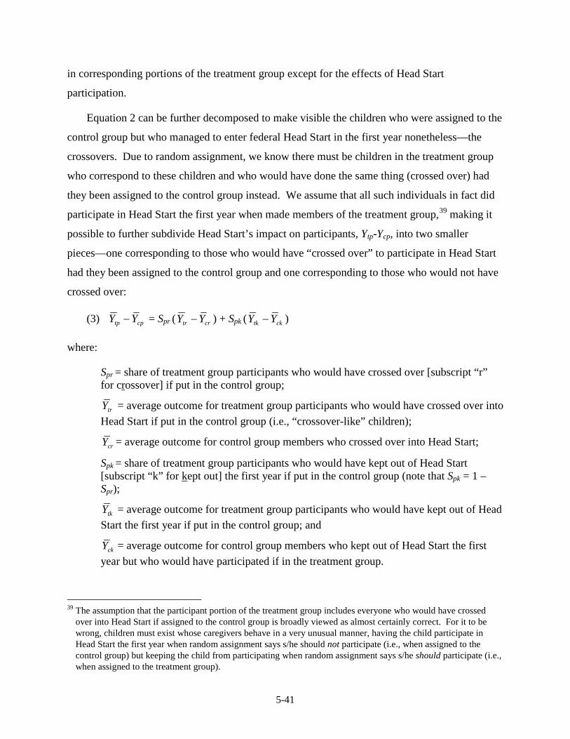
5-41
in corresponding portions of the treatment group except for the effects of Head Start
participation.
Equation 2 can be further decomposed to make visible the children who were assigned to the
control group but who managed to enter federal Head Start in the first year nonetheless—the
crossovers. Due to random assignment, we know there must be children in the treatment group
who correspond to these children and who would have done the same thing (crossed over) had
they been assigned to the control group instead. We assume that all such individuals in fact did
participate in Head Start the first year when made members of the treatment group,39
(3)
making it
possible to further subdivide Head Start’s impact on participants, Ytp-Ycp, into two smaller
pieces—one corresponding to those who would have “crossed over” to participate in Head Start
had they been assigned to the control group and one corresponding to those who would not have
crossed over:
cptp YY − = Spr ( crtr YY − ) + Spk ( cktk YY − )
where:
Spr = share of treatment group participants who would have crossed over [subscript “r” for crossover] if put in the control group;
trY = average outcome for treatment group participants who would have crossed over into Head Start if put in the control group (i.e., “crossover-like” children);
crY = average outcome for control group members who crossed over into Head Start;
Spk = share of treatment group participants who would have kept out of Head Start [subscript “k” for kept out] the first year if put in the control group (note that Spk = 1 – Spr);
tkY = average outcome for treatment group participants who would have kept out of Head Start the first year if put in the control group; and
ckY = average outcome for control group members who kept out of Head Start the first year but who would have participated if in the treatment group.
39 The assumption that the participant portion of the treatment group includes everyone who would have crossed
over into Head Start if assigned to the control group is broadly viewed as almost certainly correct. For it to be wrong, children must exist whose caregivers behave in a very unusual manner, having the child participate in Head Start the first year when random assignment says s/he should not participate (i.e., when assigned to the control group) but keeping the child from participating when random assignment says s/he should participate (i.e., when assigned to the treatment group).

5-42
Substituting Equation 3 into Equation 2, we get:
(4) I ITT = ct YY − = Sp [ Spr ( crtr YY − ) + Spk ( cktk YY − ) ] + Sn [ cntn YY − ].
The cktk YY − piece of the right-hand side of this equation compares universally treated children
to universally non-treated children, i.e., it is an IOT estimate. This piece of the overall ITT
estimate, often referred to as the “average complier effect,”40
cktk YY −
describes Head Start’s impact on
children who (a) participate in Head Start when put in the treatment group and (b) do not
participate in Head Start when put in the control group, a group called “compliers” with the
randomized design. The term in Equation 4 is the one IOT impact estimate that
follows directly from random assignment—i.e., it compares a set of children who universally
participated in Head Start ( tkY
ckY
) with an equivalent set of children who universally did not
participate ( ). But it is a portion of the ITT estimate that cannot ordinarily be identified in
the data, since the tkY
ckY
cnY
subset of the treatment group cannot be distinguished from the trY
cktk YY −
subset
(since both participate in Head Start the first year), and the subset of the control group
cannot be distinguished from the subset (since neither participates in Head Start the first
year).
The Instrumental Variable Approach to Addressing Crossovers
While it cannot be found directly in the data, the logical equivalent to can be
inferred under certain circumstances. The conventional way of doing this is to apply an
“instrumental variable” (IV) methodology that focuses on extracting impact information from the
portion of the sample for which participation in Head Start varies depending on randomization
status. Angrist, Imbens, and Rubin (2004) have shown in the statistical/econometric literature
that an IV methodology produces an unbiased estimate of the causal effect of the intervention on
compliers. Subsequently, evaluators have noted the equivalence of this method to a more
intuitive approach in which the ITT estimate is rescaled to reflect what one can infer is the
40 See, for example, Barnard, J.; Frangakis, C.; Hill, J.; & Rubin, D. (2003). Principal stratification approach to
broken randomization experiments: A case study of school choice vouchers in New York City. Journal of the American Statistical Association, 98, 299-323.

5-43
intervention’s average impact on compliers through an exercise that conceptually removes the
non-compliers.41
Looking again at Equation 4, suppose it were true that
We will take this more transparent approach here.
(5) crtr YY −
cntn YY −
ct YY −
= 0 ,
meaning that outcomes are the same for crossovers and their non-identifiable equivalents in the
treatment group. Suppose also that
(6) = 0 ,
meaning that outcomes are the same for no-shows and their non-identifiable equivalents in the
control group. Within the context of random assignment to treatment, these two equations can
be true only if Head Start has the same impact on crossovers as it does on their equivalents in the
treatment group, and the same impact—presumably, no impact at all—on no-shows and their
equivalents in the control group, since outcomes cannot differ systematically between matched
segments of the treatment and control groups except due to the impact of the intervention.
Substituting Equations 5 and 6 into Equation 4 yields the following:
(7) I ITT = Sp [ Spk ( cktk YY − ) ] .
Here we see that under the conditions in Equations 5 and 6, the “intention to treat” impact
estimate equals the difference in mean outcomes between compliers in the treatment group and
compliers in the control group, factored downward to reflect that compliers are only a share (Spk)
of the total number of children who participate in Head Start the first year if assigned to the
treatment group and that the full set of the children who participate the first year if assigned to
the treatment group are only a share (Sp) of all children assigned to the treatment group. Using
the relationships between subgroup shares given in the definitions of the different S terms above,
Equation 7 can be rewritten as
(8) I ITT = (1 – Sn) (1 – Spr) ( cktk YY − )
41 See for example Gennetian, L.A., Morris, P.A., Bos, J.M., and Bloom, H.S. Constructing instrumental variables
from experimental data to explore how treatments produce effects, p. 86, in Learning More from Social Experiments (2005), edited by H.S. Bloom. New York: Russell Sage Foundation.

5-44
This expression makes clear that the ITT estimate is “watered down” by inclusion of children
who pass through random assignment but who, based on Equations 5 and 6, experience no net
impacts from the intervention. In particular, the crossovers in Equation 5 diminish the average
ITT impact by a factor 1–Spr < 1 determined by their prevalence in the control group, Spr, while
the no-shows in Equation 6 further diminish the already diminished impact by a factor 1–Sn < 1
determined by their prevalence in the treatment group, Sn.
Returning to Equation 7, replace Spk with 1 – Spr based on the definitions given at
Equation 3 above:
(9) I ITT = Sp [ (1 - Spr ) ( cktk YY −
cktk YY −
cktk YY −
)].
A further substitution can be made based on the definition of Spr. If Sr is the share of control
group that participated in Head Start in the first year (i.e., the share that are crossovers), Spr can
be rewritten as:
(10) Spr = Sr / Sp.
It follows that
(11) 1 – Spr = (Sp – Sr ) / Sp.
Making this substitution in Equation 9,
(12) I ITT = Sp [(Sp – Sr ) / Sp ] ( ) = (Sp – Sr ) ( cktk YY − ).
Dividing Equation 12 by Sp – Sr and reversing the order of the terms gives an IOT
estimate of :
(13) cktk YY − = I ITT / (Sp – Sr).
This simply rescales the original ITT estimate by dividing by the difference in Head Start
participation rates between the treatment and control groups, i.e., by the share of the total
population that are “compliers.” This is computationally equivalent to the Angrist-Imbens-
Rubin IV estimator and, under the assumptions in Equations 5 and 6 (which parallel the Angríst-
Imbens-Rubin assumptions), unbiased as a measure of the impact of participation on the
“compliers” population.
5-45
For reasons discussed below, we use this methodology to estimate the impacts of Head
Start on participants presented in the Final Report. As noted there, any statistically significant
estimate of impact of access to Head Start is statistically significant for the impact of
participation, and any non-significant impact is non-significant. This follows for several reasons,
which collectively imply that the same p-values apply to the IOT estimates of participation
effects as the ITT estimates of access effects. (Recall that p-values indicate the probability of
obtaining an estimate of impact equal to or greater than the observed impact estimate when the
null hypothesis of no impact is true.) Tables of results in Chapters 4 through 7 (for ITT
estimates) and Appendix E (for IOT estimates) of the Final Report reflect this. Hence, they
provide the same evidence for accepting or rejecting the respective null hypotheses of the two
different analyses:
H0 ITT: Average impact of access to Head Start = 0
H0 IOT: Average impact of participating in Head Start = 0.
The basis for equating hypothesis test results between these two analyses starts with the logic of
the null hypotheses themselves and the assumptions made in obtaining IOT impact estimates
through IV methods. Specifically, equations 5 and 6, on which the IV findings rest, say that no
part of the outcome difference between the entire treatment group and the entire control group—
i.e., no part of the impact of access to Head Start—occurs among the “always takers” in equation
5 and no part of it occurs among the “never takers” in equation 6. Any impact of access that
does occur must occur among “compliers”, the remaining members of the study population who
participate in Head Start if assigned to the treatment group and who do not participate if assigned
to the control group. Thus, within the framework needed to do IV analysis, H0 ITT is true
according to whether or not compliers are affected by Head Start participation. However, within
the same framework H0 IOT is also true according to whether or not compliers are affected by
Head Start participation. Why? Because impacts on all participants have to be assumed the
same as impacts on compliers to use the IV analysis framework (see discussion of equation 14
below). Hence, the two null hypotheses are logically equivalent. It follows that whatever the
data can tell us about the veracity of one in a hypothesis testing and p-value mode must be what
it can tell us about the other.

5-46
At a more technical statistical level, the estimates used to test H0 ITT and to H0
IOT, given
in equations 1 and equation 13 differ only through division of the latter by Sp – Sr. If this
quantity is taken as a constant, with no sampling variability of its own, the standard errors of the
two estimates also differ in exactly the same way, meaning that the t-statistics for testing the two
null hypotheses—the ratio of the estimate to its standard error—are identical (as are the p-
values). If instead one looks at Sp – Sr as a random variable in its own right, adopting the
position that p-values and hypothesis test conclusions are the same for the ITT and IOT analyses
amounts to asserting that the sampling error in the observed compliance rate, Sp – Sr, is not of an
important magnitude. Heckman et al. (1998) have found this to be the case when large samples
are involved. Moreover, one can show that even with Sp – Sr, considered a random variable, the
standard error of the IOT impact estimate I ITT / (Sp – Sr) in equation 13 asymptotically
approaches the standard error of the I ITT impact estimate in equation 1 divided by the observed
Sp – Sr value in the sample as sample size goes infinite. This again makes t-statistics, p-values,
and hypothesis test inferences the same between the two types of analyses.
Other Methodologies and Their Limitations
As noted earlier, two other methodologies were considered for dealing with crossovers,
beyond the IV approach:
Remove crossovers from the analysis sample, treating them like survey “non-respondents,” and estimating impacts using a non-response adjustment that tries to offset their absence.
Compute lower and upper bounds on the IOT impact by making high- and low-end assumptions about the outcomes of crossovers would have been had they not participated in Head Start the first year.
Treating the crossovers as non-respondents would raise the overall “non-response” rate
for the control group from 20 percent to 34 percent in spring 2003 for 3-year-olds and from 23
percent to 37 percent in spring 2003 for 4-year-olds, and to a similar extent in later years (i.e.,
Spring 2004, 2005, and 2006). This would make the control group non-response rate in each
round of impact analysis much higher than the treatment group non-response rate that year,
which is 11 percent in spring 2003 for 3-year-olds and 13 percent in spring 2003 for 4-year-olds,
and similar in later years. With a high nonresponse rate, the responding subset of the control
group is no longer a valid comparison for the treatment group. Nonresponse weights cannot be
5-47
relied upon to adequately compensate for the bias in the responding subset, leading us to reject
this methodology. From the beginning, the National Head Start Impact Study was to be
conducted as a randomized control trial, in order to guarantee that the sample used to represent
Head Start participants absent the program be statistically equivalent to the group used to
represent Head Start participants with the program. This has been achieved for the entire control
group and the entire treatment group and should not be sacrificed now by “retro-fitting” the
latter. Pre-existing differences between the children removed and those retained—and hence
between the retained control group members and the full treatment group to which former would
be compared—on factors not equilibrated through the non-response weighting adjustments (such
as parental commitment to their children’s pre-kindergarten intellectual development) would
almost certainly lead to biased IOT impact estimates. Or at least raise questions about the
reliability of the IOT estimates and whether they could be considered “experimental” in nature in
any sense (and hence free of selection bias following non-response adjustment).
To do the bounding approach, assumptions have to be made about how high or low
crossover outcomes could have been had those children not participated in Head Start. While it
is possible to identify plausible “best case” and “worse case” extremes for these unmeasured
values, this approach has several limitations:
The IOT “lower bound” and “upper bound” impact estimates produced are complex to explain and difficult to compute accurately;
The upper bound portion of the strategy can only be applied to cognitive outcomes, limiting the IOT analysis to just that domain and omitting information on the impact of participating for social-emotional, health, and parenting outcomes;42
Reporting that Head Start’s impact on participants is some unknown point in a range of numbers (i.e., in the interval between the lower and upper bounds) may be unsatisfying to policy makers.
Given these weaknesses, the greatest strength of the bounding approach—that the approximate
nature of its findings conveys the reality that the randomized experiment cannot provide totally
conclusive measures of the impact of participation—did not justify its use in our judgment.
42 This is because the upper bound methodology relies on the assumption that the outcome involved has a natural
upward trajectory, so that one can assume that outcomes of crossovers in Spring 2003—had those children not participated in Head Start—would have been at least as good as the last observed outcomes for those children without Head Start in Fall 2002. For cognitive outcomes, expected to grow with time on average, this seems a justifiable assumption. But not for outcomes in the other three domains, where an upward developmental trajectory over time cannot be assumed as the norm.
5-48
Validity of and Sensitivity to the IV Assumptions
We turn now to the question of whether the assumptions needed to construct the IOT
estimate in Equation 13 are likely to be met. The earlier discussion of no-shows addressed the
assumption in Equation 6 that outcomes are the same for no-shows and their control group
counterparts, neither of which participated (for even a day) in Head Start in the year following
random assignment. Based on the initial equivalence of these two sets of children and their
universal lack of exposure to Head Start services, this is considered a very sound assumption.
Not so for the assumption in Equation 5, that outcomes of crossovers, crY
trY
, and outcomes
of their counterparts in the treatment group, , are the same. One can only count on this
assumption being met if crossovers receive the same Head Start intervention they would have
received had they been randomized into the treatment group. Given the potential that crossover
children entered the program through a more indirect or surreptitious route, and possibly with a
time lag, it is essential to scrutinize this assumption carefully. One question is whether crossover
children were served by different Head Start grantees than the one to which their families
initially applied, since at that center they were supposed to be excluded from the program
following the random assignment lottery. If so, the assumption that these children benefited
from Head Start to the same extent as the corresponding children in the treatment group (who
almost all participated at their centers of random assignment, if they participated in Head Start at
all during the first year) becomes more fragile. For 63 percent of the crossovers in the 3-year-old
sample and 59 percent of the crossovers in the 4-year-old sample the center of Head Start
participation matched the center of random assignment, greatly alleviating this concern.
Another concern pertains to the timing of Head Start participation following
randomization. Since, by the evidence in the previous paragraph, most crossover children
participated at a center that had agreed to exclude them, it is possible that they were served later
than they would have been if put in the treatment group—i.e., that the decision to break the rules
of the study design and enroll them may have taken some time to take place, leading crossovers
to make a delayed entry into the program compared to their treatment group counterparts The
data again provide some reassurance on this point: as shown in Exhibit 5.7, the distribution of
start dates for crossovers is virtually the same as for other participants (i.e., for children who
participated in Head Start after being assigned to the treatment group):
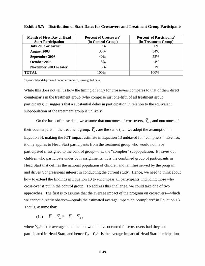
5-49
Exhibit 5.7: Distribution of Start Dates for Crossovers and Treatment Group Participants
Month of First Day of Head Start Participation
Percent of Crossoversa (in Control Group)
Percent of Participantsa (in Treatment Group)
July 2003 or earlier 9% 6% August 2003 33% 34% September 2003 40% 55% October 2003 5% 4% November 2003 or later 3% 1%
TOTAL 100% 100% a3-year-old and 4-year-old cohorts combined, unweighted data.
While this does not tell us how the timing of entry for crossovers compares to that of their direct
counterparts in the treatment group (who comprise just one-fifth of all treatment group
participants), it suggests that a substantial delay in participation in relation to the equivalent
subpopulation of the treatment group is unlikely.
On the basis of these data, we assume that outcomes of crossovers, crY
trY
crcr YY −
, and outcomes of
their counterparts in the treatment group, , are the same (i.e., we adopt the assumption in
Equation 5), making the IOT impact estimate in Equation 13 unbiased for “compliers.” Even so,
it only applies to Head Start participants from the treatment group who would not have
participated if assigned to the control group—i.e., the “complier” subpopulation. It leaves out
children who participate under both assignments. It is the combined group of participants in
Head Start that defines the national population of children and families served by the program
and drives Congressional interest in conducting the current study. Hence, we need to think about
how to extend the findings in Equation 13 to encompass all participants, including those who
cross-over if put in the control group. To address this challenge, we could take one of two
approaches. The first is to assume that the average impact of the program on crossovers—which
we cannot directly observe—equals the estimated average impact on “compliers” in Equation 13.
That is, assume that:
(14) * = cktk YY − ,
where Ycr* is the average outcome that would have occurred for crossovers had they not
participated in Head Start, and hence Ycr - Ycr* is the average impact of Head Start participation

5-50
on crossovers compared to no participation. The same concept of Head Start’s average impact
on crossovers can also be carried over to the average effect of Head Start on all treatment group
participants in Equation 3:
(15) ( cptp YY −
cptp YY −
cptp YY −
cktk YY −
cptp YY −
)* = Spr ( crtr YY −
cktk YY −
cktk YY −
cptp YY −
cptp YY −
*) + Spk ( cktk YY −
cktk YY −
crtr YY −
),
where ( )* is the average effect of Head Start on all treatment group participants
compared to outcomes for the same children had none of them participated in the program.
Substituting terms based on Equation 14, this becomes
(16) ( )* = Spr ( ) + Spk ( ) = cktk YY −
cktk YY −
,
the last step from the fact that (as noted in the definition of Spk at Equation 3 above) Spk = 1 – Spr .
Thus, when Equation 13 gives us an unbiased estimate of , the average impact on
“compliers,” it simultaneously gives us an unbiased estimate of the average impact of Head Start
on all participants, ( )* under the assumptions in Equations 5 and 14.
However, we see no basis for assuming impacts on crossovers and “compliers” are
necessarily equal. Crossovers may be a strongly self-selected and/or program-selected subset of
all would-be participants in the control group, the ones who manage to participate even in the
face of a study design and random assignment lottery outcomes that says they should not. It is
quite possible that they differ from the remaining would-be participants (i.e., the “compliers”, to
which directly applies) on factors that would lead to a greater (or smaller) ability to
benefit from Head Start’s services.
Alternatively, one could examine how large the desired impact estimate for all treatment
group participants, ( )*, would be for different true values of Ytr - Ycr*. Equation 15,
restated in equation 17 with the substitution for Spk just noted, serves as a good basis for doing
this:
(17) ( )* = Spr ( *) + (1 – Spr) ( ).

5-51
Based on the formula for Ytk - Yck in Equation 13 and using Equation 10, this can be rewritten as
(18) ( cptp YY −
crtr YY −
crtr YY −
crtr YY −
cktk YY −
crtr YY −
crtr YY −
crtr YY −
crtr YY −
crtr YY −
cktk YY − =
I ITT / (Sp – Sr ). In all, knowing Sp, Sr , and I ITT is sufficient for conducting this sensitivity
analysis.
Applying this approach separately to the 3-year-old cohort and the 4-year-old cohort in
the first year of the impact analysis (Spring 2003) illustrates the sensitivity of the IOT findings to
different unknown values of crtr YY −
)* = Spr ( crtr YY −
crtr YY −
cktk YY −
*) + (1 – Spr) [I ITT / (Sp – Sr)]
= ( Sr / Sp ) ( *) + I ITT / (1 – Sn )
= [ Sr ( *) + I ITT ] / Sp.
Sr and Sp in this formula are the share of the treatment group members who participated in
Head Start in the first year and the share of control group members who participated in Head
Start in the first year, both observed in the data. I ITT is the main impact finding from Chapters 4
through 7 of the Head Start Impact Study Final Report (U.S. Department of Health and Human
Services, January 2010). This leaves *, the impact of Head Start on crossovers
compared to their outcome levels had they not participated in Head Start, as the only unmeasured
piece of the IOT impact estimate. To address this, we do a sensitivity analysis that assumes a
variety of different values for *, each determined as a fraction of the measured impact of
Head Start on “compliers”, :
Scenario A: * = 0 ( cktk YY −
cktk YY −
cktk YY −
cktk YY −
cktk YY −
(
) = 0
Scenario B: * = 0.5 ( )
Scenario C: * = 1.0 ( ) =
Scenario D: * = 1.5 ( )
Scenario E: * = 2.0 ( )
cktk YY − ) for this purpose is derived from observable quantities using Equation 13:
*. We do this for two of the most central cognitive
outcomes in the study, PPVT and WJ-III Letter Word Identification, as shown in Exhibits 5.8
and 5.9.
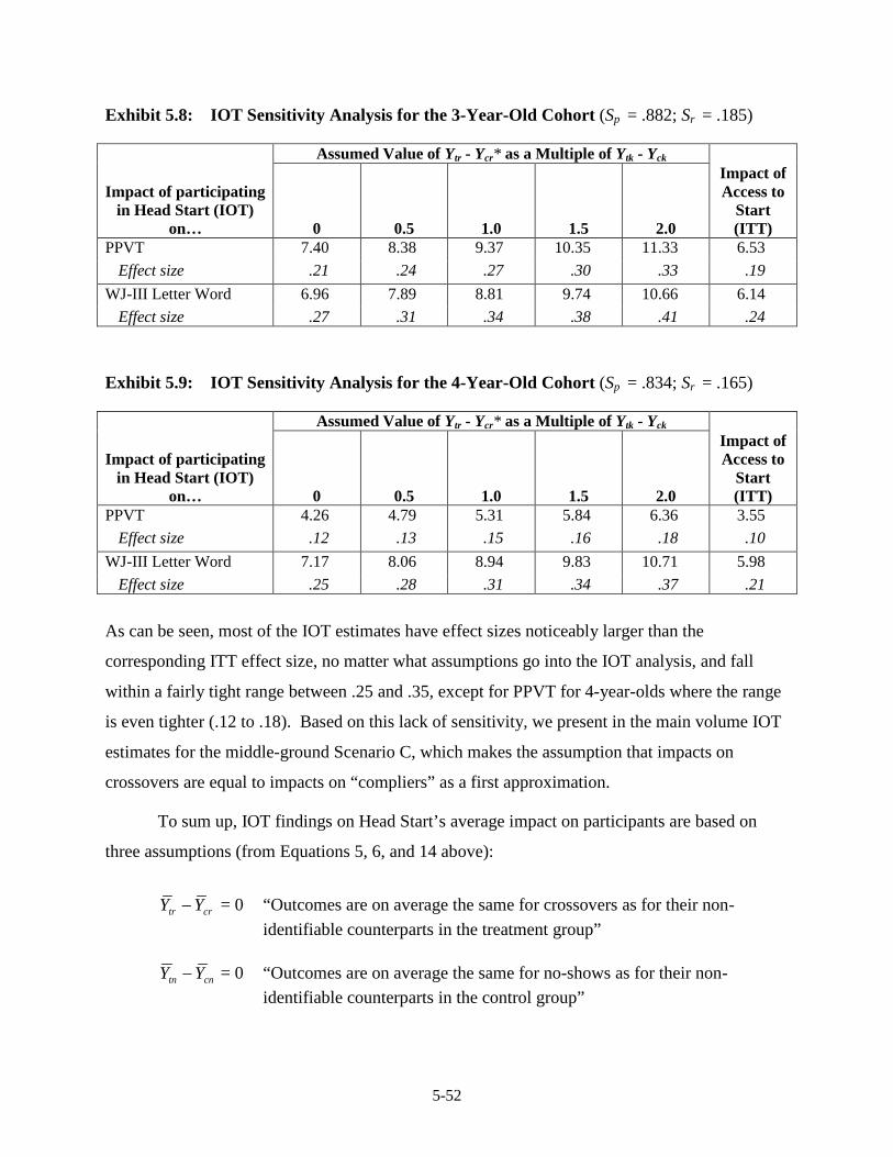
5-52
Exhibit 5.8: IOT Sensitivity Analysis for the 3-Year-Old Cohort (Sp = .882; Sr = .185)
Assumed Value of Ytr - Ycr* as a Multiple of Ytk - Yck
Impact of participating in Head Start (IOT)
on… 0 0.5 1.0 1.5 2.0
Impact of Access to
Start (ITT)
PPVT 7.40 8.38 9.37 10.35 11.33 6.53 Effect size .21 .24 .27 .30 .33 .19
WJ-III Letter Word 6.96 7.89 8.81 9.74 10.66 6.14 Effect size .27 .31 .34 .38 .41 .24
Exhibit 5.9: IOT Sensitivity Analysis for the 4-Year-Old Cohort (Sp = .834; Sr = .165)
Assumed Value of Ytr - Ycr* as a Multiple of Ytk - Yck
Impact of participating in Head Start (IOT)
on… 0 0.5 1.0 1.5 2.0
Impact of Access to
Start (ITT)
PPVT 4.26 4.79 5.31 5.84 6.36 3.55 Effect size .12 .13 .15 .16 .18 .10
WJ-III Letter Word 7.17 8.06 8.94 9.83 10.71 5.98 Effect size .25 .28 .31 .34 .37 .21
As can be seen, most of the IOT estimates have effect sizes noticeably larger than the
corresponding ITT effect size, no matter what assumptions go into the IOT analysis, and fall
within a fairly tight range between .25 and .35, except for PPVT for 4-year-olds where the range
is even tighter (.12 to .18). Based on this lack of sensitivity, we present in the main volume IOT
estimates for the middle-ground Scenario C, which makes the assumption that impacts on
crossovers are equal to impacts on “compliers” as a first approximation.
To sum up, IOT findings on Head Start’s average impact on participants are based on
three assumptions (from Equations 5, 6, and 14 above):
crtr YY −
cntn YY −
= 0 “Outcomes are on average the same for crossovers as for their non-identifiable counterparts in the treatment group”
= 0 “Outcomes are on average the same for no-shows as for their non-
identifiable counterparts in the control group”

5-53
crtr YY − * = cktk YY − “Average impact on crossovers is the same as average impact on ‘compliers’”.
The first of these assumptions is supported by the data, the second is unobjectionable on
principle, and the third does not materially affect conclusions when altered to a considerable
extent in the sensitivity analysis.
Annual Cross-Sectional Impact Estimation Methods – Subgroups
Research Questions
All of the above procedures address Head Start’s impact on the full set of children and
family types that are provided access to Head Start, looking at average impacts for the diverse
set of children and families. However, impacts are likely to vary across different subsets of the
children and families served. For example, Head Start may benefit children whose primary
language is not English more than other children (or the reverse), or it may benefit families at the
high end of the household risk index more than other families (or the reverse). In addition to an
interest in the overall national impact of Head Start, Congress mandated an examination of how
impacts vary for different types of children and families. The intent is to understand “what
drives the overall impacts” when the program is having an effect of important magnitude for the
participant population as a whole. In addition, there is interest in determining the extent to which
the benefits of Head Start may be widespread – i.e., whether the benefits reach many types of
children and families to produce the overall average effect, rather than benefiting some but
having little or no effect on others.
Identifying subgroups of children (or families) that benefit more or less from Head Start
may have important policy and program implications. It can suggest areas where the program
needs to be strengthened or enhanced to ensure that all participants advance in their
development. For example, Head Start programs are required to serve children with special
needs so it is important to understand the extent to which these children benefit from their
participation over and above an interest in determining if Head Start improves the lives of the
average participant. In addition, prior early childhood research has indicated that some groups of
children follow different developmental paths and may, as a consequence, be assisted by Head

5-54
Start in distinctive ways, such as children from racial and ethnic minority families and non-
English speaking children.
This interest in “who benefits?” motivates two types of analyses. The first considers the
impact of Head Start on individual subgroups of program participants, asking for example: Does
Head Start help children from Hispanic families? Children who start in the lowest quartile of
cognitive development scores for Head Start participants? Special needs children? A full set of
results defined on these and other dimensions, when considered as a group, will also indicate
whether (a) certain subgroups “drive” the overall average impact findings or (b) widespread
benefits accrue to many different subgroups.
The second set of analyses involving subgroups considers whether impacts differ in
magnitude between distinct types of children and families. For example, Head Start may have
smaller effects on children who initially speak little English or larger effects when primary
caregivers exhibit depressive symptoms at baseline. Interest in the comparative magnitude of
impacts stems from several sources:
Researchers want to know what factors “moderate” the influence of early childhood services (such as those provided by Head Start) on child development and family functioning. In this case, the term “moderate” means alter the size of the impact of those services when they are provided to one type of child (or family) versus another. For example, the extent to which a child’s primary caregiver reports symptoms of depression may moderate how much Head Start is able to help him/her develop good social skills, or a child’s primary language may moderate the program’s ability to expand reading readiness.
As noted above, Congress required that the study identify the types of children and families that benefit most from Head start participation, a question that implicitly relates impacts for one type of child/family to impacts for another. For example, do younger children benefit more than older children? Or do families where parents face multiple risk factors benefit more than other families?
Head Start program operators might seek to enhance services in ways that would particularly benefit subgroups found to be experiencing smaller impacts than other subgroups, such as children with special needs or families with diverse ethnic or linguistic backgrounds
With sufficient data, all subgroup impacts would become apparent when the difference in
outcomes between treatment and control group families are compared across subgroups. But
because data are limited, the study cannot decisively answer all questions about Head Start’s
impact on different subpopulations. Still, where evidence is strong that an impact on a particular

5-55
subgroup or a difference in impacts between subgroups has occurred, the subgroup analysis will
produce a finding that is not difficult to interpret: real impacts in the measured direction have
taken place with high probability.
In contrast, a non-significant finding is more ambiguous and could indicate either: (1)
that there is in fact no impact, or difference in impact, for some subgroup(s); or (2) that impacts
exist but are too small in magnitude to reach the threshold of what the sample is able to detect.
Controlling for Multiple Comparisons in the Subgroup Analyses
The subgroup analyses examined impacts on all of the child and parent outcomes for
each of the subgroups (listed below in Exhibit 5.10), for each age cohort, and for each study
year. As discussed above, when conducting such “multiple comparisons” there is a modest
probability that a finding of a statistically significant difference will emerge by random
chance―an event that is known in the statistical field as a “false discovery.” To guard against
the drawing of firm conclusions generated by false discoveries, the evaluation team statistically
adjusted the p-values using the Benjamini-Hochberg (1995) procedure described in the section
on the main impact analysis. The results of these adjustments are reported in the report chapters
along with the “basic” statistical tests.
Subgroup Definitions
Exhibit 5.10 lists the subgroups defined for the analysis to be presented in the Final
Report. All were identified in advance of any data analysis, and chosen on the basis of their
program and policy importance to the Office of Policy, Research and Evaluation/Administration
for Children and Families (OPRE/ACF), on past Head Start and child development research, and
recommendations from the Advisory Committee on Head Start Research and Evaluation. As a
precautionary measure, the distributions of the treatment and control groups were compared at
baseline with respect to the subgroup variables to ensure that they did not differ significantly
before using them for subgroup analysis. Such differences could lead to confounding of the
estimated Head Start impacts with the subgroup distributions.43
43 One of the subgroup variables, Parental Risk Index, did show a significant difference between treatment and
control groups for the age 3 cohort: 8 percent of the treatment group vs. 5 percent of the control group are in the high risk category (p = .017).
In the subgroup analysis, each

5-56
spring outcome used in the overall impact analysis is examined for each subgroup, separately by
age cohort.
Exhibit 5.10: Variables Used To Define Subgroups, Measured At Baseline
Child’s Pre-Academic Skills (Lowest Quartile/Not Lowest Quartile) Child’s Home Language (English Speaking/Dual Language Learner) Special Needs (Special Needs/Not Special Needs) Biological Mother/Caregiver Race/Ethnicity (White, Black, Hispanic) Parent-Caregiver Report Depressive Symptoms (No/Mild/Moderate/Severe Household Risk Index (Low/No, Moderate, High) Urbanicity (Urban/Not Urban)
A description of the subgroups used in the analyses is provided below.
Child’s Pre-Academic Skills—based on whether the child scored in the lowest quartile of the study population on the baseline assessment of the Woodcock-Johnson III Pre-Academic Skills (comprising of three tests: Letter-Word Identification, Spelling, and Applied Problems). Two subgroups were created using this test score: the child was in the lowest quartile subgroup, or the child was not in the lowest quartile subgroup.
Child’s home language—based on the language in which the child was assessed for the baseline assessment in fall 2002. Two subgroups were created: the child was English speaking, or the child was a Dual Language Learner (See Chapter 3 in this volume and Chapter 2 in the Final Report for how the language for the baseline assessment was determined.) The agreement between the child’s testing language and home language is very high (see Exhibit 5.11).
Special needs—based on the parent’s response to the following question on the baseline interview, “Did a doctor or other health or education professional ever tell you that [CHILD] has any special needs or disabilities—for example, physical, emotional, language, hearing, learning difficulty, or other special needs?” Two subgroups were created: the child was reported to have special needs, or the child was not reported to have special needs.
Biological mother/caregiver race/ethnicity—based on the race of the person identified as being most responsible for the care of the child at the time of the baseline parent interview.44 Three categories were created: White or other,45
44 The primary caregiver is the child’s biological mother for 96 percent of the study children.
Black, and Hispanic. There was a very high correlation between the child and the biological mother’s or primary caregiver’s race/ethnicity (see Exhibit 5.11).
45 Other race (N=94 for the 3-year-old cohort and N=85 for the 4-year-old cohort) was combined with White because the number of other race respondents was too small to study independently.

5-57
Parent/caregiver-reported depressive symptoms—determined from responses to the baseline parent/caregiver interview using the shortened version (12 items) of the Center for Epidemiologic Studies-Depression scale (CES-D) (Seligman, 199346
Household risk index—determined by the number of the following characteristics reported in the baseline parent interview: (1) receipt of TANF or Food Stamps, (2) neither parent in household has high school diploma or a GED, (3) neither parent in household is employed or in school, (4) the child’s biological mother/caregiver is a single parent, and (5) the child’s biological mother was age 19 or younger when child was born. A child’s family score could range from 0 to 5 points. Three categories were created: low/no risk (0-2 risk factors), moderate risk (3 risk factors), and high risk (4-5 risk factors).
). Four subgroups were created from the scale: (1) no depressive symptoms (score of 0-4), (2) mild depressive symptoms (score of 5-9), (3) moderate depressive symptoms (score of 10-14), and (4) severe depressive symptoms (score of 15-36).
Urbanicity—based on the location of the Head Start center at which the family applied for admission. If the center was located in a Census-defined urbanized area, the family was considered to live in an urban area; if not, the family was considered not to live in an urban area. Thus, two subgroups were defined.
Exhibit 5.11: Agreement between Race of Child and Biological Mother/Caregiver, and
between Child Testing Language and Home Language Agreement between child and biological mother/caregiver race/ethnicity (e.g., of those children who are white, what % have mothers who are white?)
Agreement between child testing language and home language (e.g., of those children tested in English, for what percent of their homes was the primary home language English?).
White/other 97% English 95% African American 98% Spanish 97% Hispanic/Latino 94% Other 87%
Lowest Quartile Determination
We elected to define the set of children who represent the “low ability” group as those
who score in the lowest quartile on one of the standardized tests that were administered by the
study team. After much discussion and review of the available baseline measures, it was
determined that the Woodcock-Johnson III Pre-Academic Standard Cluster (which includes the
following tests: Letter-Word Identification, Spelling, and Applied Problems) provides the best
definition of lowest quartile for the Fall 2002 English-English group. The cluster is designed to
measure broad achievement by assessing pre-reading and letter-word identification skills, 46 The four depressive symptoms categories are reported on page 101 in the above reference for the 20 item CES-D.
The cut points were proportionately adjusted for the shortened version of the CES-D for use in ECLS-B, FACES, and HSIS.

5-58
developing mathematical skills, and skill in written production. Exhibit 5.12 provides the
distribution for the Fall 2002 Pre-Academic Standard Cluster scores. It should be noted that the
25th percentile cutoff score is for the Head Start Impact Study sample. It is not the 25th percentile
score for the publisher’s normed population of 3-year-olds or 4-year-olds.
Exhibit 5.12: Distribution of the Pre-Academic Standard Cluster W-ability
Scores for the English-English Group, Fall 2002
Cohort Range 25th Percentile Score 3-year-olds 286-396 319 4-year-olds 286-403 341
Thus all 3-year-olds with a W-ability score of 319 or lower are included in the lowest quartile
group. Likewise, all 4-year-olds with a W ability score of 341 or lower are included in the
lowest quartile group.
For the fall 2002 Spanish-English47
group we use the parallel Bateria Woodcock-Munoz-
R Skills Cluster (which includes the following tests: Letter-Word Identification, Dictation and
Applied Problems) to determine the lowest quartile. This cluster is similar to the Woodcock-
Johnson III Pre-Academic Standard Cluster described above. Exhibit 5.13 provides the
distribution for the Fall 2002 Skills cluster scores.
Exhibit 5.13: Distribution of the Pre-Academic Standard Cluster W-ability Scores for the Spanish-English Group, Fall 2002
Cohort Range 25th Percentile Score
3-year-olds 277.7-400.3 347.6 4-year-olds 293.7-424.7 363.7
Thus all 3-year-olds with a W-ability score of 347.6 or lower are included in the lowest quartile
group. Likewise, all 4-year-olds with a W ability score of 363.7 or lower are included in the
lowest quartile group.
47 In Fall 2002, a Language Decision Form was used to determine the best language for administering the child
assessment. For children residing on the US mainland, if Spanish was determined to be their language of assessment, the children were administered a Spanish assessment with two English subtests (PPVT and Woodcock-Johnson Letter-Word Identification). In subsequent data collections, the Spanish-English group children were administered an English assessment with two Spanish subtests (TVIP and Bateria Woodcock-Munoz Letter-Word Identification). This procedure allows us to measure the child’s growth in Spanish and English across all data collection points.

5-59
Children who spoke a language other than English or Spanish are not included in the
lowest quartile analysis. The other language group children (n = 57) were administered only
non-standardized tests (e.g., Color Identification, Counting Bears, etc.) in fall 2002.
Impact Estimation Formulas for Subgroups
A computationally efficient and statistically powerful way to compare subgroups utilizes
the impact regression equations discussed earlier. For a given subgroup, a single regression can
provide information on how large an impact Head Start has on each of the subgroup categories,
and how impacts vary across subgroup categories. This analysis interacts the indicator variable
for assignment to the Head Start group with each subgroup-defining covariate in turn (or with
each set of subgroup-defining covariates when a given dimension defines more than two
subgroups such as mother’s race/ethnicity), allowing impact to vary with that factor.
To formalize this, let Z represent the subgroup-defining variable (e.g., a 0/1 indicator for
children with special needs) or a set of subgroup-defining variables (e.g., two out of three
subgroup indicator variables that divide the sample by mother’s race/ethnicity). As before T is
the treatment indicator, X the vector of demographic covariates and time of assessment variable
(if included), and R the “residualized” fall measure. As in the main impact analysis, if the
residualized fall measure is entered separately by language group, the R term in the model is
replaced by L (the language subgroup indicator, L=1 for English, L=0 for Spanish/Other) and its
two-way interaction with R. For outcomes taken from the teacher survey and teacher child rating
form, the model omits the R and L terms entirely since there is no pre-test measure for these
outcomes. (Note that Z may or may not have been among the covariates previously included in
the regressions as part of the vector of background variables, X; if not, it is added now to the
regression for the estimation of subgroup impacts.) For continuous outcomes, the impact
regression model for the ith child becomes
( )i i i i i i i iY T R Z Z T eα β δ η ζ= + + + + + +'γ X
ln ( )1
ii i i i i i
i
PT R Z Z T
Pα β δ η ζ= + + + + +
−'γ X
For binary outcomes the impact model is:
where,

5-60
'i i i i i i
i i 'i i i i i i
exp( Tγ X R Z ( Z T ))P Pr(Y 1)1 exp( Tγ X R Z ( Z T ))
α β δ η ζα β δ η ζ+ + + + +
= = =+ + + + + +
.
Continuous Outcome Measures
For continuous outcomes, all estimation, model fitting and hypothesis testing for
subgroup analysis (as was true of the main analysis) was done with the SUDAAN software
package, using the full-sample and jackknife replicate weights to take into account the complex
sample design (i.e., stratification, clustering and weighting) in the estimation of standard errors
for the regression coefficients and the impact estimates. To see how this methodology produces
impact estimates for subgroups and tests of differences in the size of impact between subgroups,
consider an example with Y as a continuous outcome variable (such as a child’s PPVT score) and
Z a two-way indicator variable distinguishing special needs children (Z=1) from non-special
needs children (Z=0):
The coeffic
( )i i i i i i i iY T R Z Z T eα β δ η ζ= + + + + + +'γ X
ients from this model used in the analysis are:
, the coefficient on the indicator variable for assignment to the treatment group, which estimates the impact of Head Start on non-special needs children, the subgroup of children not flagged by the subgroup indicator variable Z (Z=0). For these children, the regression equation reduces to Yi = α + βTi + γ'Xi + δRi + ei, paralleling the equation used previously to determine impacts on all children.
+ ζ, the estimate of the impact of Head Start on special needs children, the subgroup of children flagged by the subgroup indicator variable Z (Z=1). For these children, the regression model becomes
β
ζ, the coefficient on the interaction of the treatment group indicator variable and the subgroup indicator variable, which estimates the difference between the impact of the intervention on special needs children (Z=1) and the impact on non-special needs children (Z=0).
β
'(ά η) ( ζ)i i i i iY T X R eβ γ δ= + + + + + + , again paralleling the equation previously used to determine impacts on all children but with different coefficients on Ti and Xi. Statistical significance tests on this linear combination of coefficients tell us whether this impact differs significantly from 0.
A further variation of the subgroup analysis occurs by replacing Z with a collection of
two or more categorical variables. This occurs when looking at subgroups defined by mother’s
race/ethnicity and the parental risk index. In both cases, we use two Z variables, call them Z1 and

5-61
Z2, which flag—for example—children with Hispanic and non-Hispanic black mothers
respectively. The continuous version of the regression equation in this instance becomes
Yi = α + βTi + γ'Xi + δRi +η1 Ζ1i + η2 Ζ2i + ζ1 (Ζ1iTi) + ζ2 (Ζ2iTi) + ei
Several coefficients from this model are used in the analysis:
β estimates the impact of Head Start on children with non-Hispanic white mothers, the subgroup of children not flagged by either subgroup indicator (the Z1i = 0, Z2i = 0 subgroup). For these children the regression equation reduces to Yi = (α + βTi + γ'Xi + δRi + ei, paralleling the equation previously used to determine impacts on all children.
β + ζ1 estimates the impact of Head Start on children with Hispanic mothers (the Z1i = 1, Z2i = 0 subgroup), for whom the regression model becomes Yi =(ά + η1) + (β + ζ1) Ti + γ'Xi + δRi + ei, paralleling the equation previously used to determine impacts on all children but with different coefficients on T and X.
+ ζ2 estimates the impact of Head Start on children with non-Hispanic black mothers (the Z1i = 0, Z2i = 1 subgroup), for whom the regression model becomes Yi =(ά + η2) + (β + ζ2) Ti + γ'Xi + δRi + ei, paralleling the equation previously used to determine impacts on all children but with different coefficients on T and X.
β
Differences in impact between various pairs of subgroups can be calculated and tested using ζ1 (Hispanic versus non-Hispanic white), ζ2 (non-Hispanic black versus non-Hispanic white), and ζ1 – ζ2 (Hispanic versus non-Hispanic black).
Binary Outcome Measures
As in the main analysis, to calculate impacts on binary outcomes for subgroups the
equation for ln (P / 1-P ) is specified just as was the equation in the continuous case (except for
the log-odds conversion of the left hand-side variable). Once estimated using logistic regression,
we again solve for P = Pr(Y =1) as an exponential translation of the log-odds ratio. From there,
the predicted marginal for the treatment group is calculated for each subgroup category by first
evaluating the Pr(Y =1) equation for each child, with the treatment indicator set to 1 for the entire
sample of respondents and the remaining variables set to their actual values for the child, to
obtain the predicted probability of the outcome for each child. The weighted average of the
predicted probabilities across children belonging to the subgroup is the treatment predicted
marginal for the subgroup. The predicted marginal for the control group is calculated similarly
for each subgroup category, with the treatment indicator set to 0 for the entire sample. The
formula for the predicted marginal is given in Graubard & Korn (1999) as:

5-62
i
n
ii
n
iiii
w
rPwrP
δ
δ
∑
∑
=
==
1
1)(ˆ
)(ˆ
iP̂
C ,nonruralT nonruralnonrural
C ,ruralT ruralrural
PPI
PPIˆˆ
ˆˆ
,
,
−=
−=
)ˆˆ()ˆˆ( ,,, C nonruralT nonruralC ,ruralT ruralnonruralrural PPPPII −−−=−
where r is the level of the causal effect variable (r = treatment or control), is the predicted
probability that the binary outcome Yi = 1 for the i-th child, with the r-th level indicator set to 1
for every record for the treatment predicted marginal, and set to 0 for every record for the control
predicted marginal,
n is the number of sampled children,
wi is the full-sample weight for the i-th child, and
δi is a dummy for the subgroup of interest (ex. 1=urban, 0=rural).
The impact estimate for a particular subgroup category is calculated as the difference
between the treatment (r = treatment) predicted marginal and the control (r = control) predicted
marginals for that subgroup category. Different subgroup categories are compared by
calculating the pairwise differences in impact estimates between the subgroup categories, i.e., the
“difference of differences”. For example, to test whether the impact of Head Start on the
likelihood of receiving dental care in the last 12 months is different for children in rural and non-
rural areas, the predicted marginals in both the treatment condition and the control condition are
calculated for the rural and non-rural and all four combinations used: treatment/rural,
treatment/non-rural, control/rural, and control/non-rural. The impact estimate for each rural/non-
rural subgroup is calculated as the difference in the respective predicted marginals:
The difference in impact estimates for rural and non-rural is calculated as:
.
The hypotheses H0: Irural = 0, H0: Inonrural = 0, and H0: Irural – Inonrural = 0 are tested using a t-
test, with the standard error of the difference or the difference of differences calculated in SAS
using the jackknife replicate weights to reflect the complex sample design. For binary outcomes,

5-63
the calculation of predicted marginals, impact estimates, and standard errors for subgroups and
the hypothesis testing of subgroup impacts and differences in impacts were programmed in SAS
using the jackknife replicate weights, as the SUDAAN software (v.9) does not subset the sample
by subgroup in calculating predicted marginals for subgroups as the Graubard & Korn formula
requires. Instead, it averages over the entire sample with the subgroup category indicator set to 1
for every record—i.e., it omits the δi 0/1 indicator for the subgroup of interest from the predicted
marginal equation. Since our goal is to compare the effect of Head Start for different subgroups,
the SUDAAN calculations are not appropriate for our analysis.
The approach described above extends to analyses of three related subgroups, such as
mother’s race/ethnicity. Here, the model becomes
)()(1
ln ** 12112 THISPANICTBLACKHISPANICBLACK1 R T p
p ζζηηδβα +++++++=−
Xγ '
)ˆˆ()ˆˆ( ,,,, ChispanicThispanicCwhiteTwhitehispanicwhite PPPPII −−−=−
)ˆˆ()ˆˆ( ,,,, CblackTblackCwhiteTwhiteblackwhite PPPPII −−−=−
)ˆˆ()ˆˆ( ,,,, CblackTblackChispanicThispanicblackhispanic PPPPII −−−=−
white, Cwhite, Tblack, Cblack, TChispanic, Thispanic, PPPPPP ˆ,ˆ,ˆ,ˆ,ˆ,ˆ
where BLACK, HISPANIC are 0,1 indicators for the mother’s race/ethnicity, and White/Other is
the omitted reference group. The impact estimates for the race/ethnicity groups are
C hispanic,T hispanic,hispanic
C black,T black, black
C white,T white,white
PPIPPIPP I
ˆˆˆˆˆˆ
−=−=
−=
and the differences in impacts among the race/ethnicity groups are:
where are the predicted marginals in
the treatment and control conditions for each race/ethnicity category.
Two final restrictions are placed on the subgroup analyses. First, to avoid findings that
may exaggerate contrasts between subgroups due to the vagaries of small-sample analysis,
subgroups with fewer than 50 observations in either the treatment or control group for any age
cohort are not examined. Second, certain observations could not be included in particular
subgroup analyses for certain moderators. In particular, children who could not be assessed in
either English or Spanish in fall 2002 due to lack of familiarity with these languages are dropped
5-64
from the analysis sample when examining subgroups based on children’s pre-academic
composite score at baseline.
Repeated-Measures Impact Analysis Methods
This section describes the derivation of the longitudinal analysis findings on cognitive
impacts presented in Chapter 4 of the Final Report using hierarchical linear modeling (HLM)
methods to estimate the effect of access to Head Start on the average annual growth rate of five
cognitive outcomes, for the three to four year follow-up period covered by the study (depending
on children’s age at entry into the program). HLM is an approach to analyzing data in nested
hierarchies that takes this clustering into account when calculating the significance tests of
estimated effects (Raudenbush and Bryk, 2002). The method is particularly well suited to
framing questions about changes over time—e.g., does cognitive development over time grow
along a steeper linear trajectory when children are given access to Head Start—because it models
at its most irreducible level the growth trajectory of individual children. This results in more
accurate estimates of changes over time in Head Start’s impact than cross-sectional impact
estimates, subject to the assumption of a linear growth rate.48
While the cross-sectional analysis of Head Start impact in any single year, using
SUDAAN software, models the clustering of children within centers and of centers within
grantees/delegate agencies in a way that yields correct standard errors for the impact estimates, it
cannot model effects that vary randomly over groups—for example, when the amount of growth
per year varies randomly from child to child. By looking at only a single year at a time, it also
cannot model the growth over time of individual children. The HLM approach on the other hand
can estimate effects that vary from center to center and it also estimates individual growth
trajectories. However, a limitation of this software is that it can incorporate only part of the
multistage stratified sample design used in the Head Start Impact Study when estimating the
standard errors of effects. The current HLM software accommodates the nesting of time points
within children and the nesting of children within centers but—unlike SUDAAN for cross-
48 If (i) all the cross-sections had identical samples (or perfect longitudinal weights were used), (ii) all the same
covariates were used at each time point, and (iii) all covariates measured perfectly, the estimate of the difference in growth rates between the treatment and control groups in the cross-sectional analysis would have the same expected value for any given outcome as the HLM estimate. Since these conditions are not met by the data, HLM gives the better measure of linear growth rates and Head Start’s impact thereon.

5-65
sectional analysis—not the nesting of centers within grantees/delegate agencies. However, a
simulation study has shown that for the types of models used here HLM yields standard errors
that are correct for treatment effect estimators (Jenkins, Lee, Cheach, & Leytush, 2006).
HLM Model Specification for the Head Start Impact Study
The application of HLM used in the Head Start Impact Study is a three-level model
which describes observations of time points within students, outcomes for students within
centers, and the distribution of center means. Suppose that Yjit is the outcome for child i in
center j measured at time point t. At level 1 of the model, this outcome is related to Wit, the
wave of data collection for child i at time t. At level 2, the initial achievement level and rate of
growth in achievement are related to a child’s background characteristics, X1ji …Xpji (e.g.
child’s gender, primary language, family composition). In addition, the rate of growth at this
level is potentially influenced by whether the student was assigned to the Head Start group or to
the non-Head Start control group. A third level of the model accounts for the clustering of
students in within centers without specifying any additional relationships among variables.
Level 1 – Time Within Students, describes the different time points of data collection for
a given child. For the age three cohort there are five waves: baseline (fall, 2002), 1st followup
(spring 2003), second followup (spring 2004), 3rd followup (Spring 2005), and final wave
(spring, 2006). For the age four cohort only the first four waves are included.
Level 1 – Time Points Within Child:
(1) Yjit = π0ji + π1ji Wjit + ejit ,
where Yjit = The outcome for child i in center j when measured at time point (i.e., data collection wave) t.
Wjit = Data collection wave in which Yjit is observed, coded 0, 1, 2, 3, 4 for the 3-year-old cohort and 0, 1, 2, 3 for the 4-year-old cohort. π0ji = The estimated initial level of achievement for child i in center j at time point 0 (i.e., in fall 2002). π1ji = The linear growth parameter for child I in center j indicating how much that
child grew in achievement between successive observation points. ejit = A random error term for child i in center j at time t.

5-66
It is assumed that the random error, ejit has variance σ2 that is fixed across all time points,
children, and centers49
Level 2 – Children Within Center, describes the way individual child characteristics
relate to the level and growth rate of child outcomes within a given Head Start center. These are
expressed as regression coefficients predicting the child-specific parameters in Level 1 of the
model, π0ji and π1ji :
and is independent of errors at other levels of the model.
(2) 0 00 01 1 0 0
1 10 11 12 1 1( 1) 1
ji j ji p pji ji
ji ji ji p pji ji
X X rT X X r
π β β β
π β β β β +
= + + + +
= + + + + +
1 jiX
11β
Where to pjiX
12 0( 1)pβ β +
is the random effect associated with child i’s baseline achievement level at center j,
0 jir
1 jir is the random effect associated with child i’s annual growth rate in achievement at center j.
are child characteristics that predict level and growth of achievement,50
Tji is an indicator of treatment condition to which child i was assigned
(0=control, 1=Head Start), which affects the growth rate of child outcomes if access to Head Start has an impact on children’s development
00 jβ
01 0 pβ βis the average baseline achievement level of children in center j,
are the fixed effects of child background characteristics on baseline achievement levels, assumed to be the same for all children and all centers, 10β is the average annual growth of child achievement across all children, assumed to be the same in every year is the impact of being assigned to the treatment group on the average annual growth of child achievement across all children, assumed to be the same in every year. This is the key estimate needed from the model, measuring Head Start’s impact on the annual growth rate of child achievement.
are the fixed effects of student covariates on child achievement growth, assumed to be the same for all children at all centers,
49 The HLM software requires this uniform residual variance assumption at the lowest level of the model. 50 This assumes that same child background characteristics influence initial achievement levels and achievement
growth. Note that for estimation purposes all covariates are grand-mean deviated.

5-67
Level 3: Between Centers (3) 00 000 00j juβ γ= +
000γ
00 ju
, where
is the average baseline achievement level of all children in all centers,
is the random effect associated with center j’s average baseline achievement level.
Interpreting the Multilevel Model
The level 1 model (Equation 1) depicts an individual growth curve, that is, it describes
how an individual’s cognitive proficiency grows over time. This is defined as linear growth
which is characterized by an initial starting point, π0ji , and a yearly increment of growth, π1ji. for
each child i in each center j. The level 2 model (Equation 2) describes how the intercepts and
slopes of the growth line (π0ji, π1ji again) vary from one child to another within a center. A
child’s intercept term, π0ji , is a function of a center mean baseline achievement level, 00 jβ
01 0 pβ β
. Similarly, the child’s rate of growth over time, , π1ji, is a function of the average growth rate
at all center,
, the
effect of various child covariates, , and a random error term for each child in center j,
0 jir
10β
, the effect of child background characteristics,
, the increment to growth due to access to Head Start following random
assignment to treatment, 11β
1 jir .
12 0( 1)pβ β +
00 jβ
(assumed
the same in all centers), and a random error term for each child in center j,
The level 3 model depicts center means, , and a
random center effect,
, as a function of a grand mean,
00 ju . As mentioned before, this part of the model is included sim
000γ
ply to
account for the clustering of students within centers.
The main focus of the HLM analysis is the effect of treatment, Tji , on students’ growth,
β11. A positive value for β11 would imply that those given access to Head Start (the treatment
group) grow in achievement more than those not given access (the control group). For example,
since time is years, if β11 has a value of three this means that for each year of follow-up, the
treatment group grows three more points than the control group on the outcome.

5-68
In other words, β12 is the estimate of the impact of treatment assignment on growth. In
addition, this impact estimate is controlled for the values of the child covariates 1 jiX to pjiX
10β̂ 11β̂ + ,
-- the estimated effect of Head Start on the average annual linear growth rate,
.
Including covariates in the model increases the statistical precision of the impact estimate.
Estimating the Multilevel Model
Longitudinal analysis is done using the above model to obtain measures of Head Start’s
“intent to treat” (ITT) impact on children’s annual growth rates for five cognitive outcomes:
PPVT and four assessments from the Woodcock Johnson III, Letter Word Identification,
Spelling, Applied Problems, and Pre-Academic Skills Composite. These measures were chosen
as the only outcomes that were collected in every year of the study that can be vertically equated
and for which steady growth is expected based on child development theory and prior research.
Like the main findings from cross-sectional analysis, each of the age cohorts is
considered separately. For each age cohort and outcome measure, the analysis sample consists
of all children for whom the outcome was observed at least two time points, which could include
the baseline “pretest” observation in fall 2002 or any of the outcome measurement points in
spring 2003, spring 2004, spring 2005, and—for the 3-year-old cohort—spring 2006. Thus, any
sample member could have from two to five observations of Yjit in the estimation sample, for t =
0, 1, 2, 3, and/or 4. This length of follow-up carries all children potentially through the end of 1st
grade, although for some the final outcome observation at that age may be missing (just as any
previous time points, so long as at least two total time points are observed).
Special longitudinal weights were constructed for this sample and used in forming all of
the estimates. These are described in Chapter 2 of this report.
Based on these samples and weights, the HLM software produced the figures presented in
Exhibits 5.4 and 4.7 of the main report for each outcome. These include the following estimates:
-- the average annual linear growth rate for children in the control group sample,
-- the average annual linear growth rate for children in the treatment group sample,
11β̂ ,
11β̂-- the p-value for , from which one can decide if the regression coefficient differences significantly from zero at the alpha = .05 level (or any other level of
5-69
significance) and hence if there is strong evidence of impact of Head Start access on children’s linear growth trajectories.
Methodological Refinements Since Previous Interim Report
In a small number of instances, the analysis methods used here differ from those used the
study’s previous impact report (U.S. Department of Health and Human Services, Administration
for Children and Families, 2005), which looked only at impacts in the first year following
random assignment. These refinements, made in situations where the study team identified ways
to improve the analytic techniques applied, account for the minor differences in findings reported
here for that year (the spring 2003 results) and in the earlier report. These refinements include
the following:
Scoring the PPVT and CTOPPP cognitive tests using separate prior distributions for the treatment and control groups and updating those priors each year from the previous year’s data.
Collapsing continuous measures of color score and number of times parents read to their children into two-way categorizations to reflect the fact that each variable took on only a few discrete values and did not have the bell-shaped (i.e., normal) curve for its distribution among sample members that estimation of impacts on continuous measures assumes. By converting each measure to a binary indicator coded one for all children above a certain threshold zero otherwise, we are able to estimate impacts using logistical methods (applied as well to other binary measures) that do not make the normality assumption.
Three refinements were made in adjusting the impact estimates to take account of background characteristics of the children and families analyzed:
o Demographic covariates measured in fall 2002 but at some interval after random assignment and (for the treatment group) Head Start program entry were limited to only those measures that could not have been affected by the program in only a few weeks. Covariates dropped because of the possibility of an early impact of Head Start are caregiver depression scale, caregiver’s self-reported health status, grandparent living in the home, number of residential moves in the last 12 months, household monthly income range, and household receipt of TANF. The indicator of a child having special needs was also dropped because of the possibility that participation in Head Start may quickly have lead to increased identification of this characteristic.
o Pre-test values of key outcome measures, when used as covariates, were “residualized” on the treatment/control group indicator variable before use—again, to protect against the possibility of the measures being systematically higher or lower for the treatment group than the control group due to an early impact of Head Start.

5-70
o A covariate was added to measure the date of testing in the spring of each year, to assure that differences in timing over the several-week data collection interval did not lead to higher outcome levels for one or the other experimental group because of later testing and, hence, greater maturation independent of the intervention due simply to aging.
Finally, estimation methods and statistical testing procedures were modified in two ways:
o For the multiple comparisons made as part of the subgroup impacts, the Benjamini-Hochberg procedure was used to reduce the likelihood of false discoveries of statistical significance.
o Average impacts were calculated using the predicted marginal methodology, rather than the direct observation of the estimated coefficient on the treatment group indictor (for continuous outcomes) and the conditional marginal methodology (for binary outcomes) used in the previous report.

5-71
References Angrist, J.D., Imbens, G.W., and Rubin, D.B. (2004). Identification of causal effects using
instrumental variables. Journal of the American Statistical Association, 9, 444-472. Benjamini, Y., and Hochberg, Y. (1995). Controlling for the false discovery rate: A practical
and powerful approach to multiple testing. Journal of the Royal Statistical Society, Series B (Methodological), 57(1): 289-300.
Bloom, H.S. (1984). Accounting for no-shows in experimental evaluation designs. Evaluation
Review, 8, 225-246. Graubard, B. and Korn, E. (1999). Predictive margins with survey data. Biometrics 55, 652-
656. Heckman, J., Smith, J., and Taber, C. (1998). Accounting for dropouts in evaluations of social
programs. The Review of Economics and Statistics, 80(1), 1-14. Jenkins, F., Lee, H., Cheah, B. & Leytush, O. (2006). Hierarchical linear modeling using
complex survey data. Presented at the Annual Joint Statistical Meetings, Seattle, WA. Pfeffermann, D., Skinner, C., Goldstein, H. & Rasbash, J. (1998). Weighting for unequal
selection probabilities in multilevel models. Journal of the Royal Statistical Society, Series B, 60(1), 23-40.
Raudenbush, S. & Bryk, A. (2002). Hierarchical linear models: Applications and data analysis
method. (Second Edition). Newbury Park, CA: Sage. Research Triangle Institute. (2005). SUDAAN user’s manual. Release 9.0. Research Triangle
Park, NC: Author. Seligman, M.E.P. (1993). What you can change…and what you can’t. New York: Ballantine
Books. U.S. Department of Health and Human Services, Administration for Children and Families.
(June 2005). Head Start Impact Study: First year findings. Washington, DC: Author.
U.S. Department of Health and Human Services, Administration for Children and Families. (January 2010). Head Start Impact Study. Final Report. Washington, DC: Author.