1

Health Monitoring of Aging Aerospace Structures using the Electro-Mechanical Impedance Method

Andrei Zagrai and Victor Giurgiutiu Mechanical Engineering Department, University of South Carolina

Columbia, SC 29208, 803-777-8018, victorg@sc.edu

ABSTRACT This paper describes the use of the electro-mechanical (E/M) impedance method for health monitoring of aging aerospace structures. As a nondestructive evaluation technology, the E/M impedance method allows us to identify the structural dynamics directly by obtaining the E/M impedance signatures of attached piezoelectric wafer active sensors (PWAS). The theoretical model for 2-D structures, which predicts the E/M impedance response at PWAS terminals, was developed and validated. The model accounts for axial and flexural vibrations of a host structure and considers both, structural dynamics and dynamics of the sensor. The study of sensor’s sensitivity to structural damage is presented. The presence of damage modifies the E/M impedance spectrum causing frequency shifts, peak splitting and appearance of new harmonics. The overall-statistics damage metrics and probabilistic neural network (PNN) were used to classify data according to damage severity. When installed on the aging aircraft panel, the sensors response features: (a) in the near field, spectral baseline change; (b) in the medium field, changes in harmonics distribution. These effects were successfully captured with overall-statistics damage metrics (correlation coefficient deviation) and PNN respectively. The health monitoring of aging aerospace specimens shows that unobtrusive permanently attached PWAS in conjunction with E/M impedance method can be successfully used to assess the presence of incipient damage through the examination and classification of the E/M impedance spectra.

Keywords: impedance method, active sensors, circular plates, aging aircraft, health monitoring, statistics, neural networks,

1. INTRODUCTION Structural health monitoring (SHM) plays a significant role in maintaining the safety of aged aerospace vehicles that are subject to heavy periodic loads. For such structures, the development of integrated sensory system able to monitor, collect, and deliver the structural health information is essential. One of the proposed approaches is to utilize PWAS array in which the local structural health can be monitored with E/M impedance method. The E/M impedance method assesses the local structural response at high frequencies (typically hundreds of kHz). It is not disturbed by the global conditions such as flight loads and ambient vibrations. Thus, the E/M impedance method allows monitoring of small-scaled phenomena (i.e., cracks, delamination, etc), whose contribution to the global dynamics of the structure may not be noticeable.

The E/M impedance method was extensively applied to SHM of various structural components and civil engineering structures. The local-area health monitoring of a tail-fuselage aircraft junction was described by Chaudhry et al. (1995). Giurgiutiu et al. (2001) used the E/M impedance method to detect a near-field damage in realistic built-up panels representative of aging aircraft structures. Recent developments in the E/M impedance method were discussed by Park and Inman, 2001. The implementation of E/M impedance method for detecting delamination and crack growth on composite reinforced concrete walls was presented. Other structures were also considered. An extensive study of the damage metrics suitable for E/M impedance SHM was presented by Tseng et al. 2001. The authors used an overall-statistics approach to quantify the presence of damage. The correlation coefficient was found to be the most appropriate damage metric.

Pioneering theoretical work on the analysis of sensor-structure interaction in E/M impedance method was presented by Liang et al. (1994) and Sun et al. (1994). Further model development was attempted by other investigators (Zhou, et al. 1996, Esteban, 1996) but none have derived explicit expressions for predicting the E/M impedance as it would be measured by the impedance analyzer at the embedded active sensor terminals. Recent advances were reported by Park, Cudney, and Inman (2000) who performed analysis for axial vibrations of a bar. While the structural dynamics was always accounted for in the solution, the majority of authors assumed that the stiffness of the piezoelectric sensor is static and no sensor dynamics was considered. Giurgiutiu and Zagrai (2002) derived an expression for the E/M admittance and impedance that incorporates both the sensor dynamics and the structural dynamics. However, the analysis was limited to 1-D structures. The present paper continues and extends this work to 2-D structures, specifically thin circular plates.

SPIE's 9th Annual International Symposium on Smart Structures and Materials and 7th Annual International Symposium on NDE for Health Monitoring and Diagnostics, 11-18 March 2002, San Diego, CA. paper # SS02 4702-33

2

2. MODELING OF PWAS – CIRCULAR PLATE INTERACTION Isotropic thin circular plates are used in the theoretical investigation. Both, axial and flexural components of natural vibrations are included in the solution. In the development, we account for the structural and the sensor dynamics and predict the E/M impedance response as it would be measured at the sensors terminals during structural identification process.

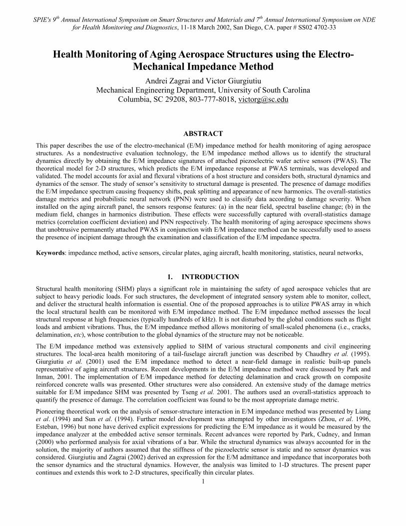
Consider a piezoelectric disk sensor placed in the center of the circular plate as it is shown in the Figure 1. For further consideration, it is convenient to formulate our problem in terms of total displacement of piezoelectric sensor bonded at the origin of the circular plate undergoing axial and flexural vibrations. When the piezoelectric sensor is excited by the external voltage with certain amplitude, the volume of a sensor expands or shrinks depending on a voltage sign. Therefore, elongation cased by electric excitation of piezoelectric material produces both: force and moment excitation of the host plate. These excitation forces and moments are derived from the PZT force, ˆ i t

PZT PZTF F e ω= using the geometry presented in Figure 1.

2a PZThM F= , a PZTN F= (1)

For harmonic excitation, we denote the total line force and line moment produced by PZT as:

( , ) ( )e a i tr rN r t N r e ω= ⋅ ( , ) ( )e a i t

r rM r t M r e ω= ⋅ (2)

Since the problem is axially symmetric, the θ-dependent component will not be considered. The magnitude of the excitation line force and line moment in Equations (2) is defined in terms of the Heaviside function:

[ ]( ) ( )ar a aN r N H r r= ⋅ − − [ ]( ) ( )a

r a aM r M H r r= ⋅ − (r Œ [0,µ) (3)

2.1 Modeling of a Circular Plate Dynamics The excitation line force and line moment expressed by Equations (2) and (3) represent an external force in the known equations for axi-symmetric axial and flexural vibration of circular plates (Leissa, 1969; Soedel, 1993; Rao, 1999):

2 2

2 2 2 21

1

e er rN NEh u u u uh

r r r rr r tρ

ν ∂∂ ∂ ∂

+ − − ⋅ = − + ∂ ∂− ∂ ∂

(4)

22

42 2

2e er rM MwD w h

r rt rρ

∂ ∂∂∇ + ⋅ = +

∂∂ ∂ (5)

where u is the radial in-plane displacement, and w is the transverse displacement. The solution of Equations (4) and (5) is expressed as series expansions in terms of modeshapes:

( , ) ( ) i tr k k

ku r t P R r e ω

= ⋅ ∑ , ( , ) ( ) i t

m mm

w r t G Y r e ω = ⋅ ⋅ ∑ , (6)

where Pk and Gm correspond to the modal participation factors of axial and flexural vibrations. The solutions for modeshapes Rk and Ym for axial and flexural vibrations of circular plate are expressed in terms of Bessel functions for particular boundary conditions (Itao and Crandall, 1979):

1( ) ( )k k kR r A J rλ= ( ) ( )0 0( )m m m m mY r A J r C I rλ λ= ⋅ + ⋅ (7)

The modeshapes Rk and Ym of Equations (7) form ortho-normal sets of functions defined by the following conditions:

2 20 0

( ) ( )a

k l klh R r R r rdrd h aπ

ρ θ ρ π δ⋅ = ⋅ ⋅∫ ∫ 2 20 0

( ) ( )a

p m pm pmh Y r Y r rdrd m a hπ

ρ θ δ π ρ δ⋅ ⋅ = ⋅ = ⋅ ⋅∫ ∫ (8)

where a is a radius of a circular plate, h is the thickness, and ρ is the density; q and n equal to zero for our particular case.

Plate

F PZT

PWAS

Plate

PWASz = h/2

r a

r

O A

F PZT

z Figure 1 Schematics on elongation of

piezoelectric sensor bounded on the plate.

3

Using expressions Equations (4)-(8), the modal participation factors for axial and flexural vibrations are obtained as:

( )

02 2 2

( ) ( ) ( )22i

aa k a k a

ak

k k

r R r R r H r r drNP

h aρ ω ς ω

− − = ⋅⋅ − +

∫ ( )

/

2 2 2

3 ( ) ( )22i

m a a m aam

m m

Y r r Y rMG

h aρ ω ς ω

+ ⋅ =⋅ − +

(9)

where ζk and ζm are the modal damping ratios.

2.2 Effective Structural Stiffness The radial displacement of piezoelectric sensor consists of axial and flexural parts:

( , ) ( , ) ( , )Axial FlexuralPZT a PZT a PZT au r t u r t u r t= + , /

0( , ) ( , ) ( , )2PZT a a ahu r t u r t w r t= − ⋅ (10)

where w(ra,t) is the bending displacements of the neutral axis. Referring to Figure 1, the difference in displacement between points A and O is

/0( , ) ( , ) (0, ) ( ) ( )

2i t i t

PZT a A a k k a m m ak m

hu r t u r t u t P R r e G Y r eω ω= − = ⋅ − ⋅∑ ∑ (11)

Substitution of Equations (9) into Equation (11) yields the following result for the axial displacement of piezoelectric active sensor:

( ) ( )

/ /0

2 2 2 2 2

( ) ( ) ( ) ( ) 3 ( ) ( ) ( )222i 2i

aa k a k a k a m a a m a m a i ta

PZTk mk k m m

r R r R r H r r dr R r Y r r Y r Y rN hu eha

ω

ρ ω ς ω ω ς ω

− − + ⋅ ⋅ = ⋅ + ⋅ ⋅ ⋅ − + − +

∫∑ ∑ (12)

The dynamic structural stiffness can be defined in terms of the line force Na and the displacement of piezoelectric active sensor. Defining the structural stiffness, ˆstr a PZTk N u= , where ˆPZTu is given by Equation (12), we obtain

( ) ( )

1/ /

022 2 2 2

( ) ( ) ( ) ( ) 3 ( ) ( ) ( )2( )22i 2i

aa k a k a k a m a a m a m a

strk mk k m m

r R r R r H r r dr R r Y r r Y r Y rhk ah

ω ρω ς ω ω ς ω

− − − + ⋅ ⋅ = ⋅ ⋅ + ⋅

− + − +

∫∑ ∑ (13)

In some cases, this result can be conveniently expressed in terms of the frequency response function i.e.,

Hstr (ω) = 1 / kstr (ω) (14)

2.3 The PZT Active Sensor Impedance The linear constitutive equations for piezoelectric material in cylindrical coordinates are (Onoe et al. 1967; Pugachev, 1984; IEEE Std, 1987):

11 12 31E E

rr rr zS s T s T d Eθθ= + + , 12 11 31E E

rr zS s T s T d Eθθ θθ= + + , ( )31 33T

z rr zD d T T Eθθ ε= + + (15)

where rr rS u r= ∂ ∂ and rS u rθθ = are the strain-displacement relationships for axi-symmetric motion expressed in terms of the radial displacement ur.

Applying Newton’s law of motion, upon substitution, one recovers the equation of motion in polar coordinates:

2 2

2 2 21 1 0r r r ru u u ur r cr r t

∂ ∂ ∂+ − − =

∂∂ ∂ (16)

where 2111/ (1 )E

ac sρ ν= ⋅ − is the sound speed in the circular PWAS for axially symmetric radial motion. The general solution of Equation (16) is expressed in terms of the Bessel functions of the first kind, J1, in the form

4

1( , ) i tr

ru r t A J ec

ωω = ⋅

(17)

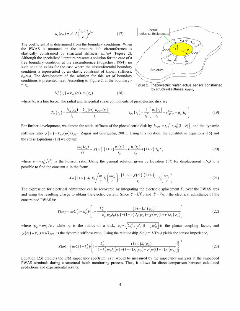
The coefficient A is determined from the boundary conditions. When the PWAS is mounted on the structure, it’s circumference is elastically constrained by structural stiffness, kstr(ω) (Figure 2). Although the specialized literature presents a solution for the case of a free boundary condition at the circumference (Pugachev, 1984), no such solution exists for the case where the circumferential boundary condition is represented by an elastic constraint of known stiffness, kstr(ω). The development of the solution for this set of boundary conditions is presented next. According to Figure 2, at the boundary r = ra,

( ) ( )( )ar a str r aN r k u rω= ⋅ (18)

where Na is a line force. The radial and tangential stress components of piezoelectric disk are:

( ) ( ) ( ) ( )a a str PZT arr a

a a

N r k u rT r

t tω ⋅

= = , ( ) ( )12 31

11

1 r a Ea rr zE

a

u rT r s T d E

rsθθ

= − −

(19)

For further development, we denote the static stiffness of the piezoelectric disk by 11(1 )EPZT a ak t r s ν = − , and the dynamic

stiffness ratio ( ) ( )str PZTk kχ ω ω= (Zagrai and Giurgiutiu, 2001). Using this notation, the constitutive Equations (15) and the stress Equations (19) we obtain:

( ) ( ) ( ) 31( ) ( ) ( )

1 1r a r a r az

a a

u r u r u rd E

r r rχ ω ν ν ν

∂= ⋅ + − + +

∂ (20)

where 12 11E Es sν = − is the Poisson ratio. Using the general solution given by Equation (17) for displacement ur(ra) it is

possible to find the constant A in the form:

( ) ( ) ( )( )31 0 0 1

1 11 a a

a

r rA d E J Jc c r c

ν χ ω νω ωων− + ⋅ + = + ⋅ − ⋅

(21)

The expression for electrical admittance can be recovered by integrating the electric displacement Dz over the PWAS area and using the resulting charge to obtain the electric current. Since ˆ ˆY I V= , and ˆ ˆ

aE V t= , the electrical admittance of the constrained PWAS is:

( ) ( ) ( )( ) ( ) ( ) ( )( ) ( )

212

20 1 1

1( ) i 1 1

1 11p a

pa a ap

k JY C k

J J Jkν ϕ

ω ωϕ ϕ ν ϕ χ ω ν ϕ

+= − ⋅ +

− − − +− (22)

where /a ar cϕ ω= , while ra is the radius of a disk, 231 11 332 / (1 )E T

p ak d s ν ε = ⋅ − is the planar coupling factor, and

( ) ( )str PZTk kχ ω ω= is the dynamic stiffness ratio. Using the relationship Z(ω) = 1/Y(ω) yields the sensor impedance,

( ) ( ) ( )( ) ( ) ( ) ( )( ) ( )

1212

20 1 1

1( ) i 1 1

1 11p a

pa a ap

k JZ C k

J J Jkν ϕ

ω ωϕ ϕ ν ϕ χ ω ν ϕ

− + = − ⋅ +

− − − +− (23)

Equation (23) predicts the E/M impedance spectrum, as it would be measured by the impedance analyzer at the embedded PWAS terminals during a structural heath monitoring process. Thus, it allows for direct comparison between calculated predictions and experimental results.

PWAS

radius ra; thickness ta

kstr

r, ur

z kstr

Structure

Ez

Figure 2 Piezoelectric wafer active sensor constrained

by structural stiffness, kstr(ω)

5

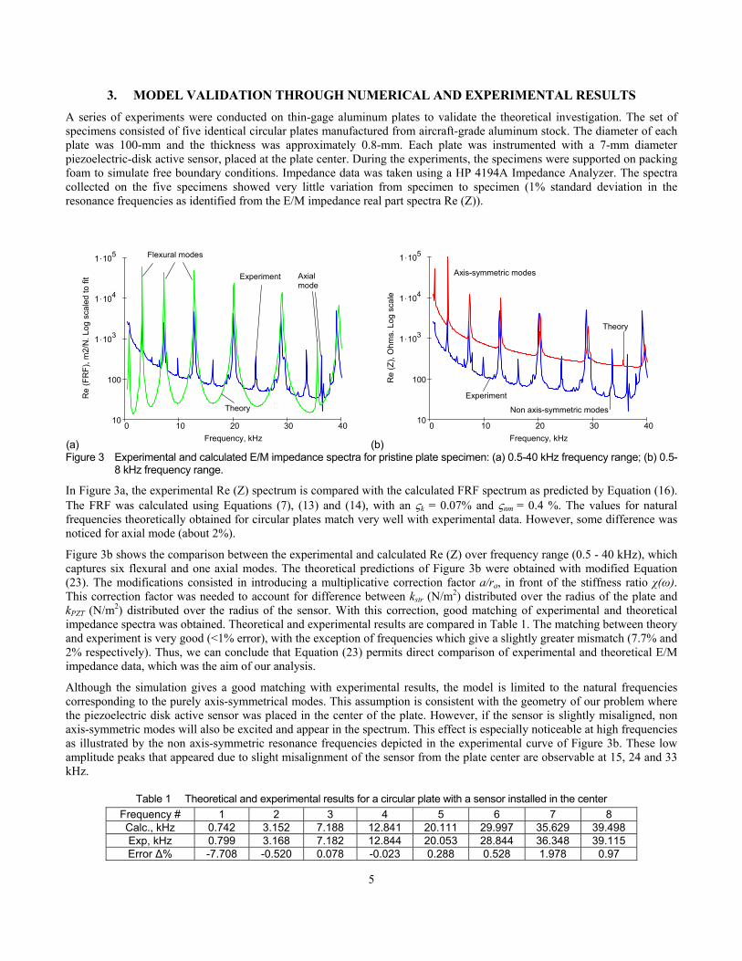
3. MODEL VALIDATION THROUGH NUMERICAL AND EXPERIMENTAL RESULTS A series of experiments were conducted on thin-gage aluminum plates to validate the theoretical investigation. The set of specimens consisted of five identical circular plates manufactured from aircraft-grade aluminum stock. The diameter of each plate was 100-mm and the thickness was approximately 0.8-mm. Each plate was instrumented with a 7-mm diameter piezoelectric-disk active sensor, placed at the plate center. During the experiments, the specimens were supported on packing foam to simulate free boundary conditions. Impedance data was taken using a HP 4194A Impedance Analyzer. The spectra collected on the five specimens showed very little variation from specimen to specimen (1% standard deviation in the resonance frequencies as identified from the E/M impedance real part spectra Re (Z)).

(a)

0 10 20 30 4010

100

1 .103

1 .104

1 .105

Frequency, kHz

Re

(FR

F), m

2/N

. Log

sca

led

to fi

t

Theory

Experiment Axial mode

Flexural modes

(b)

0 10 20 30 4010

100

1 .103

1 .104

1 .105

Frequency, kHz

Re

(Z),

Ohm

s. L

og s

cale

Axis-symmetric modes

Theory

Experiment

Non axis-symmetric modes

Figure 3 Experimental and calculated E/M impedance spectra for pristine plate specimen: (a) 0.5-40 kHz frequency range; (b) 0.5-

8 kHz frequency range.

In Figure 3a, the experimental Re (Z) spectrum is compared with the calculated FRF spectrum as predicted by Equation (16). The FRF was calculated using Equations (7), (13) and (14), with an ςk = 0.07% and ςnm = 0.4 %. The values for natural frequencies theoretically obtained for circular plates match very well with experimental data. However, some difference was noticed for axial mode (about 2%).

Figure 3b shows the comparison between the experimental and calculated Re (Z) over frequency range (0.5 - 40 kHz), which captures six flexural and one axial modes. The theoretical predictions of Figure 3b were obtained with modified Equation (23). The modifications consisted in introducing a multiplicative correction factor a/ra, in front of the stiffness ratio χ(ω). This correction factor was needed to account for difference between kstr (N/m2) distributed over the radius of the plate and kPZT (N/m2) distributed over the radius of the sensor. With this correction, good matching of experimental and theoretical impedance spectra was obtained. Theoretical and experimental results are compared in Table 1. The matching between theory and experiment is very good (<1% error), with the exception of frequencies which give a slightly greater mismatch (7.7% and 2% respectively). Thus, we can conclude that Equation (23) permits direct comparison of experimental and theoretical E/M impedance data, which was the aim of our analysis.

Although the simulation gives a good matching with experimental results, the model is limited to the natural frequencies corresponding to the purely axis-symmetrical modes. This assumption is consistent with the geometry of our problem where the piezoelectric disk active sensor was placed in the center of the plate. However, if the sensor is slightly misaligned, non axis-symmetric modes will also be excited and appear in the spectrum. This effect is especially noticeable at high frequencies as illustrated by the non axis-symmetric resonance frequencies depicted in the experimental curve of Figure 3b. These low amplitude peaks that appeared due to slight misalignment of the sensor from the plate center are observable at 15, 24 and 33 kHz.

Table 1 Theoretical and experimental results for a circular plate with a sensor installed in the center Frequency # 1 2 3 4 5 6 7 8 Calc., kHz 0.742 3.152 7.188 12.841 20.111 29.997 35.629 39.498 Exp, kHz 0.799 3.168 7.182 12.844 20.053 28.844 36.348 39.115 Error ∆% -7.708 -0.520 0.078 -0.023 0.288 0.528 1.978 0.97

6

4. DAMAGE DETECTION IN CIRCULAR PLATES Systematic experiments were performed to assess the crack detection capabilities of the method. The experiment is shown in Figure 4. Five groups of “identical” circular plates were considered: one group consisted of pristine plates (Group 0) and four groups consisted of plates with simulated cracks placed at increasing distance from the plate edge (Group 1 through 4). In our study, a 10-mm circumferential slit was used to simulate an in-service crack. During the experiments, the specimens were supported on packing foam to simulate free boundary conditions.

The experiments were conducted over three frequency bands: 10-40 kHz; 10-150 kHz, and 300-450 kHz. The data was process by capturing the real part of the E/M impedance spectrum, and determining a damage metric to quantify the difference between two spectra. Figure 4 shows data in the 10-40 kHz band. The superposed spectra of groups 0 through 4 specimens are shown in Figure 4 according to the damage location. When the damage is located in the close proximity of the sensor, the real part of the E/M impedance spectrum is drastically modified. Resonant frequency shifts, peaks splitting, and the appearance of new resonances are noticed. For the high frequency bands, similar results were obtained.

10

100

1000

10000

10 15 20 25 30 35 40

Frequency, kHz

Re

Z, O

hms

Damage Severity

Distance between crack and PWAS

40 mm

25 mm

10 mm

3 mm

pristine Group 0

Group 1

Group 2

Group 3

Group 4

Figure 4 Dependence of the E/M impedance spectra on the location of damage

4.1 Overall-Statistics Damage Metrics The damage index is a scalar quantity resulted in processing of two impedance spectra and reveals the difference between them. Theoretically, the best damage index would be a metric, which captures features of the spectra directly modified by the damage presence, and neglects the variations due to normal conditions. (i.e. statistical difference within one population of specimens or normal deviation of temperature, pressure, ambient vibrations etc). To date, several damage metrics are used to compare impedance spectra and assess the damage presence. Among them, the most popular are: the root mean square deviation (RMSD), the mean absolute percentage deviation (MAPD), and the correlation coefficient deviation (CCD). The mathematical expressions for these metrics are given in terms of impedance real part Re (Z) as follows:

2 20 0Re( ) Re( ) / Re( )i i i

N NRMSD Z Z Z = − ∑ ∑ , (24)

0 0Re( ) Re( ) / Re( )i i iN

MAPD Z Z Z = − ∑ , (25)

CCD = 1 – CC, where 0

0 01 Re( ) Re( ) Re( ) Re( )i iNZ Z

CC Z Z Z Zσ σ

= − ⋅ − ∑ , (26)

7

Table 2 Overall-statistics damage metrics for various frequency bands Frequency

band 11-40 kHz 11-150 kHz 300-450 kHz

Compared groups 0_1 0_2 0_3 0_4 0_1 0_2 0_3 0_4 0_1 0_2 0_3 0_4

RMSD, % 122 116 94 108 144 161 109 118 93 96 102 107

MAPD, % 107 89 102 180 241 259 170 183 189 115 142 242

CCD, % 84 75 53 100 93 91 52 96 81 85 87 89

300-450kHz band

45.4%37.5%

32.0%

23.2%

1%0%

20%

40%

60%

3 10 25 40 50

Crack distance, mm

(1-C

or.C

oeff.

)^7

%

Figure 5 Monotonic variation of the CCD7 damage metric with the crack radial position on a 50-mm radius plate in the 300—450 kHz band

where N is the number of sample points in the spectrum and the superscript 0 signifies the pristine state of the structure. Z , 0Z are the mean values and Zσ , 0Zσ are the standard deviations for the current and the pristine spectra.

Equations (24)-(26) result in a scalar number, which represent the relationship between the compared spectra. Thus, we expect that the variations in impedance real part, Re(Z), and appearance of new harmonics may alter the scalar value of damage index identifying the damage. The advantage of using Equations (24) – (26) is that the input impedance spectrum does not need any pre-processing, i.e., the data obtained from measurement equipment can be directly used to calculate the damage index. In our experimental study, we used the scalar values of RMSD, MAPD, and CCD calculated with Equations (24) – (26) to classify the different groups of specimens presented in Figure 4. The results of the calculations are summarized in the Table 2. We found the correlation coefficient deviation to be the best metric of damage presence. Table 2 presents correlation coefficient deviation for three frequency bands: 10-40kHz, 10-150kHz, 300-450 kHz. It was observed that for the10-40kHz and 10-150kHz frequency ranges distribution of variation of correlation coefficient is not uniform, although it was expected to decrease as the crack moves away from the sensor. The choice of frequency band for data analysis plays significant role in classification process; the frequency band with highest density of peaks is recommended. Following this approach, the frequency band 300-450 kHz was chosen for further data analysis. The variation of correlation coefficient, CCD7, was studied for 4 damage scenarios. The results are presented in Figure 5. The CCD7 damage metric tends to linearly decrease as the crack moves away from the sensor.

4.2 Implementation of PNN for Damage Identification in Circular Plates Specimen Probabilistic neural networks (PNN) were first proposed by Specht (1990) as an efficient tool for solving classification problems. In contrast to other neural networks algorithms used for damage identification (Lopes et al. 2000), PNN has statistically-derived activation function and utilizes Bayesian decision strategy for the classification problem. The kernel-based approach to probability density function (PDF) approximation is used. This was introduced by Parzen (1962) and allows one to construct a PDF of any sample of data without any a priori probabilistic hypothesis (Rasson and Lissoir, 1998). The reconstruction of the probability density is achieved by approximating each sample point with kernel function(s) to obtain a smooth continuous approximation of the probability distribution (Dunlea et al. 2001). In other words, using kernel technique it is possible to map a pattern space (data sample) into the feature space (classes). However, the result of such transformation should retain essential information presented in the data sample and be free of redundant information, which may contaminate the feature space. In this study, we used resonance frequencies of the circular plate as a data sample to classify spectra into five classes according to the damage severity. The classical multivariate Gaussian kernel was chosen for PNN implementation. In the original Specht’s formulation (Specht, 1990), this kernel was expressed as:

( )( )

( ) ( )2 2

1

1 exp22

TnAi Ai

A d di

x x x xp x

n σπ σ =

− − = − ⋅

∑ (27)

where i is a pattern number, xAi is ith training pattern from A category, n is total number of training patterns, d is dimensionality of measurement space, and σ is a spread parameter. Although the Gaussian kernel function was used in this work, its form is generally not limited to being Gaussian. Burrascano et al. (2001) utilized a PNN with different kernel types for damage identification.

To construct the input vectors for PNN, the spectra shown on Figure 4 was processed to obtain the dominant resonance

8

frequencies for each correspondent class. As it was discussed above, we have five classes (groups 0 through 4) of specimens, as depicted in Figure 4. At the beginning, a small number of frequencies was used, namely the 4 dominant frequencies of the pristine plate. The PNN used for this case consists of 4 inputs, 5 neurons in pattern layer and 5 neurons in output layer. The number of inputs corresponds to number of frequencies in the input features vector, the pattern layer is formed according to numbers of input/target pairs, and the number of output neurons represents categories in which the input data supposed to be classified. Initially, a one out of five vectors within each class was used for training. The PNN was able to successfully classify the inputs that represent high and intermediate damage levels (groups 2,3,4 vs. group 0). However, when the damage was weak (group 1 vs. group 0), the PNN produces inconsistent results. As the number of training vectors was increased for these groups, the incidence of misclassification diminished. However, even for the maximum number of training vectors (four), misclassification error between group 0 and group 1 could not be avoided.

To solve this problem, the number of frequencies in the input vectors was increased to six. One input vector from each group of specimens was used for training. Due to additional information, the PNN even distinguished the most difficult classification cases, i.e. the weak damage class (group 1) vs. the pristine class (group 0). Regardless of the choice of training vector, all input data was correctly classified into the five classes. In the discussed examples, only the deviation of natural frequencies from the original value correspondent to healthy structure was considered. The appearance of new harmonics was not introduced yet. Nevertheless, this feature plays an important role in distinguishing healthy and damaged structures especially for the cases when the damage is incipient or located far away from the sensor. It is possible to account for the appearance of new harmonics by introducing the zero values for frequencies in the feature vector of a healthy structure where these harmonics were not present. This method allows expanding the feature vector to the desired length. As an example, eleven frequencies were used in the input feature vectors to create a network. Similar to the previous situation, the PNN was able to correctly classify data regardless of the choice of the training vector. Figure 6 presents the percent of correct classified data vs. number of features in the input vectors of PNN. The good classification results obtained with PNN encourage further use of the method for damage classification in actual structures.

(a)

10 mm

94 mm

PWAS

S 6 S 2

S 5 S 1

Panel 0

Riv

ets

Riv

ets

(b)

10 mm

94 mm

PWAS

Other cracks

12 mm crack

Tentative near field

Tentativemedium field

S 8 S 4

S 7 S 3

Panel 1

Riv

ets

Riv

ets

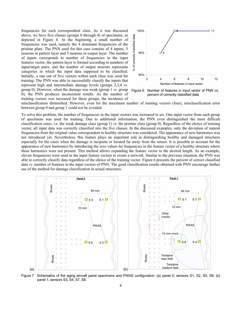
Figure 7 Schematics of the aging aircraft panel specimens and PWAS configuration: (a) panel 0, sensors S1, S2, S5, S6; (b) panel 1, sensors S3, S4, S7, S8.

4

6 11

80%

90%

100%

2 4 6 8 10 12Number of features in input vector

% o

f cor

rect

ly c

lass

ified

dat

a

Figure 6 Number of features in input vector of PNN vs.

percent of correctly classified data

9

5. DAMAGE IDENTIFICATION IN AGING AIRCRAFT PANELS Realistic specimens representative of real-life aerospace structures with aging-induced damage (cracks and corrosion) were developed at Sandia National Laboratories. Figure 7 presents a portion of the experimental panel typical of conventional aircraft structures. The whole specimen construction is made of 1-mm (0.040”) thick 2024-T3 Al-clad sheet assembled with 4.2-mm (0.166”) diameter countersunk rivets. Cracks were simulated with Electric Discharge Machine (EDM). In our study we investigated crack damage and considered two specimens: pristine “panel 0” and with cracks “panel 1”.

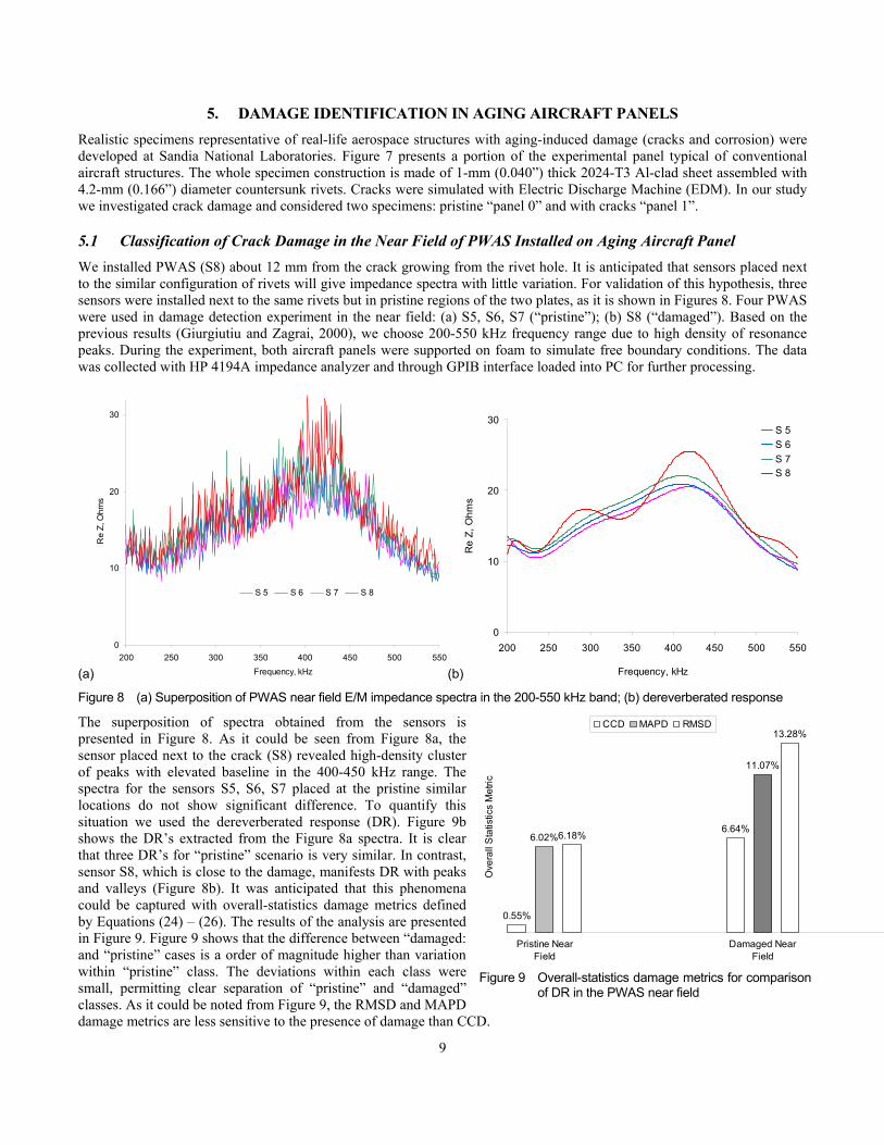
5.1 Classification of Crack Damage in the Near Field of PWAS Installed on Aging Aircraft Panel We installed PWAS (S8) about 12 mm from the crack growing from the rivet hole. It is anticipated that sensors placed next to the similar configuration of rivets will give impedance spectra with little variation. For validation of this hypothesis, three sensors were installed next to the same rivets but in pristine regions of the two plates, as it is shown in Figures 8. Four PWAS were used in damage detection experiment in the near field: (a) S5, S6, S7 (“pristine”); (b) S8 (“damaged”). Based on the previous results (Giurgiutiu and Zagrai, 2000), we choose 200-550 kHz frequency range due to high density of resonance peaks. During the experiment, both aircraft panels were supported on foam to simulate free boundary conditions. The data was collected with HP 4194A impedance analyzer and through GPIB interface loaded into PC for further processing.

(a)

0

10

20

30

200 250 300 350 400 450 500 550Frequency, kHz

Re

Z, O

hms

S 5 S 6 S 7 S 8

(b)

0

10

20

30

200 250 300 350 400 450 500 550

Frequency, kHz

Re

Z, O

hms

S 5S 6S 7S 8

Figure 8 (a) Superposition of PWAS near field E/M impedance spectra in the 200-550 kHz band; (b) dereverberated response

The superposition of spectra obtained from the sensors is presented in Figure 8. As it could be seen from Figure 8a, the sensor placed next to the crack (S8) revealed high-density cluster of peaks with elevated baseline in the 400-450 kHz range. The spectra for the sensors S5, S6, S7 placed at the pristine similar locations do not show significant difference. To quantify this situation we used the dereverberated response (DR). Figure 9b shows the DR’s extracted from the Figure 8a spectra. It is clear that three DR’s for “pristine” scenario is very similar. In contrast, sensor S8, which is close to the damage, manifests DR with peaks and valleys (Figure 8b). It was anticipated that this phenomena could be captured with overall-statistics damage metrics defined by Equations (24) – (26). The results of the analysis are presented in Figure 9. Figure 9 shows that the difference between “damaged: and “pristine” cases is a order of magnitude higher than variation within “pristine” class. The deviations within each class were small, permitting clear separation of “pristine” and “damaged” classes. As it could be noted from Figure 9, the RMSD and MAPD damage metrics are less sensitive to the presence of damage than CCD.

0.55%

6.64%6.02%

11.07%

6.18%

13.28%

Pristine NearField

Damaged NearField

Ove

rall

Sta

tistic

s M

etric

CCD MAPD RMSD

Figure 9 Overall-statistics damage metrics for comparison

of DR in the PWAS near field

10

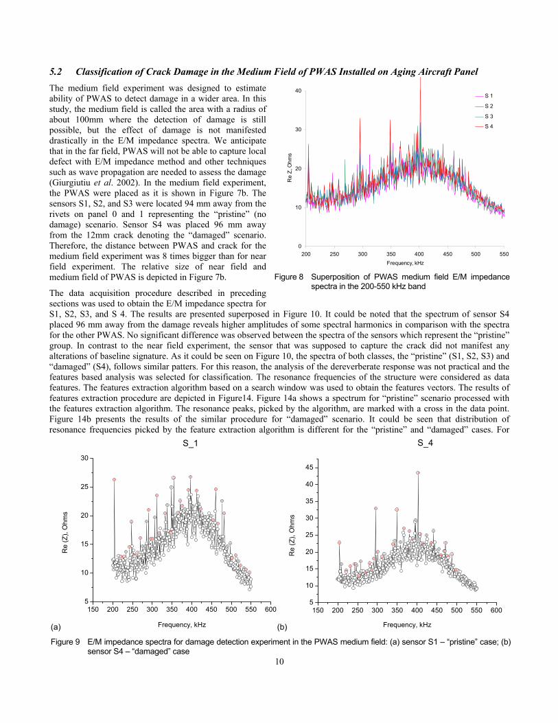
5.2 Classification of Crack Damage in the Medium Field of PWAS Installed on Aging Aircraft Panel The medium field experiment was designed to estimate ability of PWAS to detect damage in a wider area. In this study, the medium field is called the area with a radius of about 100mm where the detection of damage is still possible, but the effect of damage is not manifested drastically in the E/M impedance spectra. We anticipate that in the far field, PWAS will not be able to capture local defect with E/M impedance method and other techniques such as wave propagation are needed to assess the damage (Giurgiutiu et al. 2002). In the medium field experiment, the PWAS were placed as it is shown in Figure 7b. The sensors S1, S2, and S3 were located 94 mm away from the rivets on panel 0 and 1 representing the “pristine” (no damage) scenario. Sensor S4 was placed 96 mm away from the 12mm crack denoting the “damaged” scenario. Therefore, the distance between PWAS and crack for the medium field experiment was 8 times bigger than for near field experiment. The relative size of near field and medium field of PWAS is depicted in Figure 7b.

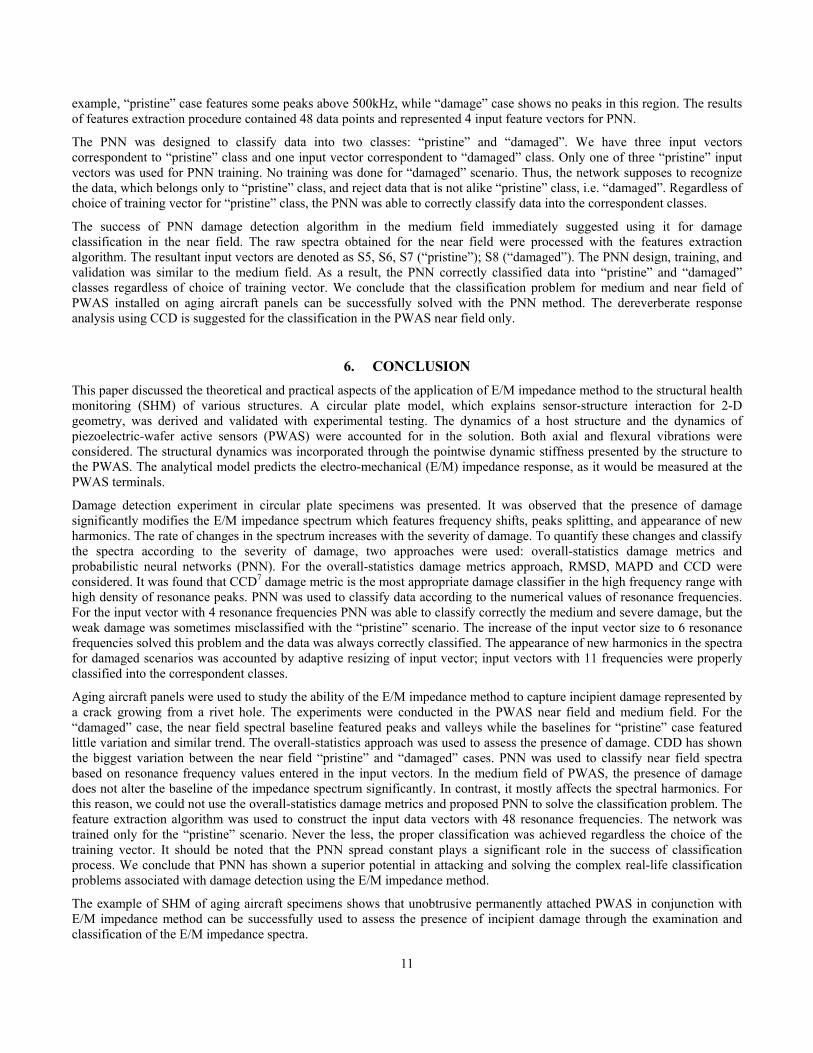
The data acquisition procedure described in preceding sections was used to obtain the E/M impedance spectra for S1, S2, S3, and S 4. The results are presented superposed in Figure 10. It could be noted that the spectrum of sensor S4 placed 96 mm away from the damage reveals higher amplitudes of some spectral harmonics in comparison with the spectra for the other PWAS. No significant difference was observed between the spectra of the sensors which represent the “pristine” group. In contrast to the near field experiment, the sensor that was supposed to capture the crack did not manifest any alterations of baseline signature. As it could be seen on Figure 10, the spectra of both classes, the “pristine” (S1, S2, S3) and “damaged” (S4), follows similar patters. For this reason, the analysis of the dereverberate response was not practical and the features based analysis was selected for classification. The resonance frequencies of the structure were considered as data features. The features extraction algorithm based on a search window was used to obtain the features vectors. The results of features extraction procedure are depicted in Figure14. Figure 14a shows a spectrum for “pristine” scenario processed with the features extraction algorithm. The resonance peaks, picked by the algorithm, are marked with a cross in the data point. Figure 14b presents the results of the similar procedure for “damaged” scenario. It could be seen that distribution of resonance frequencies picked by the feature extraction algorithm is different for the “pristine” and “damaged” cases. For

0

10

20

30

40

200 250 300 350 400 450 500 550Frequency, kHz

Re

Z, O

hms

S 1

S 2

S 3

S 4

Figure 8 Superposition of PWAS medium field E/M impedance

spectra in the 200-550 kHz band

(a)

150 200 250 300 350 400 450 500 550 6005

10

15

20

25

30

S_1

Re

(Z),

Ohm

s

Frequency, kHz (b)

150 200 250 300 350 400 450 500 550 6005

10

15

20

25

30

35

40

45

S_4

Re

(Z),

Ohm

s

Frequency, kHz Figure 9 E/M impedance spectra for damage detection experiment in the PWAS medium field: (a) sensor S1 – “pristine” case; (b)

sensor S4 – “damaged” case

11

example, “pristine” case features some peaks above 500kHz, while “damage” case shows no peaks in this region. The results of features extraction procedure contained 48 data points and represented 4 input feature vectors for PNN.

The PNN was designed to classify data into two classes: “pristine” and “damaged”. We have three input vectors correspondent to “pristine” class and one input vector correspondent to “damaged” class. Only one of three “pristine” input vectors was used for PNN training. No training was done for “damaged” scenario. Thus, the network supposes to recognize the data, which belongs only to “pristine” class, and reject data that is not alike “pristine” class, i.e. “damaged”. Regardless of choice of training vector for “pristine” class, the PNN was able to correctly classify data into the correspondent classes.

The success of PNN damage detection algorithm in the medium field immediately suggested using it for damage classification in the near field. The raw spectra obtained for the near field were processed with the features extraction algorithm. The resultant input vectors are denoted as S5, S6, S7 (“pristine”); S8 (“damaged”). The PNN design, training, and validation was similar to the medium field. As a result, the PNN correctly classified data into “pristine” and “damaged” classes regardless of choice of training vector. We conclude that the classification problem for medium and near field of PWAS installed on aging aircraft panels can be successfully solved with the PNN method. The dereverberate response analysis using CCD is suggested for the classification in the PWAS near field only.

6. CONCLUSION This paper discussed the theoretical and practical aspects of the application of E/M impedance method to the structural health monitoring (SHM) of various structures. A circular plate model, which explains sensor-structure interaction for 2-D geometry, was derived and validated with experimental testing. The dynamics of a host structure and the dynamics of piezoelectric-wafer active sensors (PWAS) were accounted for in the solution. Both axial and flexural vibrations were considered. The structural dynamics was incorporated through the pointwise dynamic stiffness presented by the structure to the PWAS. The analytical model predicts the electro-mechanical (E/M) impedance response, as it would be measured at the PWAS terminals.

Damage detection experiment in circular plate specimens was presented. It was observed that the presence of damage significantly modifies the E/M impedance spectrum which features frequency shifts, peaks splitting, and appearance of new harmonics. The rate of changes in the spectrum increases with the severity of damage. To quantify these changes and classify the spectra according to the severity of damage, two approaches were used: overall-statistics damage metrics and probabilistic neural networks (PNN). For the overall-statistics damage metrics approach, RMSD, MAPD and CCD were considered. It was found that CCD7 damage metric is the most appropriate damage classifier in the high frequency range with high density of resonance peaks. PNN was used to classify data according to the numerical values of resonance frequencies. For the input vector with 4 resonance frequencies PNN was able to classify correctly the medium and severe damage, but the weak damage was sometimes misclassified with the “pristine” scenario. The increase of the input vector size to 6 resonance frequencies solved this problem and the data was always correctly classified. The appearance of new harmonics in the spectra for damaged scenarios was accounted by adaptive resizing of input vector; input vectors with 11 frequencies were properly classified into the correspondent classes.

Aging aircraft panels were used to study the ability of the E/M impedance method to capture incipient damage represented by a crack growing from a rivet hole. The experiments were conducted in the PWAS near field and medium field. For the “damaged” case, the near field spectral baseline featured peaks and valleys while the baselines for “pristine” case featured little variation and similar trend. The overall-statistics approach was used to assess the presence of damage. CDD has shown the biggest variation between the near field “pristine” and “damaged” cases. PNN was used to classify near field spectra based on resonance frequency values entered in the input vectors. In the medium field of PWAS, the presence of damage does not alter the baseline of the impedance spectrum significantly. In contrast, it mostly affects the spectral harmonics. For this reason, we could not use the overall-statistics damage metrics and proposed PNN to solve the classification problem. The feature extraction algorithm was used to construct the input data vectors with 48 resonance frequencies. The network was trained only for the “pristine” scenario. Never the less, the proper classification was achieved regardless the choice of the training vector. It should be noted that the PNN spread constant plays a significant role in the success of classification process. We conclude that PNN has shown a superior potential in attacking and solving the complex real-life classification problems associated with damage detection using the E/M impedance method.

The example of SHM of aging aircraft specimens shows that unobtrusive permanently attached PWAS in conjunction with E/M impedance method can be successfully used to assess the presence of incipient damage through the examination and classification of the E/M impedance spectra.

12

ACKNOWLEDGMENTS The financial support of Department of Energy through the Sandia National Laboratories, contract doc. # BF 0133 is thankfully acknowledged. Sandia National Laboratories is a multi-program laboratory operated by Sandia Corporation, a Lockheed Martin Company, for the United States Department of Energy under contract DE-AC04-94AL85000.

REFERENCES Burrascano, P., Cardelli, E., Faba, A., Fiori, S., Massinelli A. (2001) “Application of Probabilistic Neural Networks to Eddy Current Non

Destructive Test Problems”, EANN 2001 Conference, 16-18 July 2001, Cagliari, Italy Chaudhry, Z., Joseph, T., Sun, F., and Rogers, C. (1995) "Local-Area Health Monitoring of Aircraft via Piezoelectric Actuator/Sensor

Patches," Proceedings, SPIE North American Conference on Smart Structures and Materials, San Diego, CA, 26 Feb. - 3 March, 1995; Vol. 2443, pp. 268-276.

Dunlea, S., Moriarty, P., Fegan, D.J. (2001) “Selection of TeV γ-rays Using the Kernel Multivariate Technique”, Proceedings of ICRC 2001

Esteban, J. (1996) “Analysis of the Sensing Region of a PZT Actuator-Sensor”, Ph. D. Dissertation, Virginia Polytechnic Institute and State University, July 1996.

Giurgiutiu, V., Zagrai, A.N, Bao J. (2002) “Piezoelectric Wafer Active Sensors (PWAS)”, Invention Disclosure to the University of South Carolina, # 00330, March 6, 2002

Giurgiutiu, V., Zagrai, A.N. (2002) "Embedded Self-Sensing Piezoelectric Active Sensors for On-line Structural Identification", Transactions of ASME, Journal of Vibration and Acoustics, January 2002, Vol.124, pp. 116-125

Giurgiutiu, V., Zagrai, A.N., Bao, J. J. (2001) "Embedded Active Sensors for In-Situ Structural Health Monitoring of Aging Aircraft Panels", Proceedings of ASME 7th Non Destructive Evaluation Topical Conference, San Antonio, Texas, 23-25 April 2001, p. 107-116

Giurgiutiu, V., Zagrai, A.N. (2000), “Damage detection in simulated aging-aircraft panels using the electro-mechanical impedance technique”, Proceedings of Adaptive Structure and Material Systems Symposium, ASME Winter annual meeting, Nov. 5-10, 2000, Orlando, FL.

IEEE Std. 176 (1987), IEEE Standard on Piezoelectricity, The Institute of Electrical and Electronics Engineers, Inc., 1987. Itao, K., Crandall, S.H. (1979) “Natural Modes and Natural Frequencies of Uniform, Circular, Free-Edge Plates”, Journal of Applied

Mechanics, Vol. 46, 1979, pp. 448-453. Liang, C., Sun, F. P., and Rogers C. A. (1994) “Coupled Electro-Mechanical Analysis of Adaptive Material System-Determination of the

Actuator Power Consumption and System energy Transfer”, Journal of Intelligent Material Systems and Structures, Vol. 5, January 1994, pp. 12-20

Liessa, A. (1969) “Vibration of Plates”, Published for the Acoustical Society of America through the American Institute of Physics, Reprinted in 1993

Lopes Jr.V.; Park, G., Cudney, H., Inman, D. (2000) "Impedance Based Structural Health Monitoring with Artificial Neural Network", Journal of Intelligent Materials Systems and Structures, Vol.11, March 2000, pp.206-214

Onoe, Mario, Jumonji, Hiromichi (1967) “Useful formulas for piezoelectric ceramic resonators and their application to Measurement of parameters”, IRE, Number 4, Part 2, 1967

Park, G., and Inman, D.J. (2001) “Impedance-based Structural Health Monitoring”, Monograph: Nondestructive Testing and Evaluation Methods for Infrastructure Condition Assessment, edited by Woo, S.C., Kluwer Academic Publishers, New York, NY, in press.

Park, G., Cudney, H. H., Inman, D. J. (2000) “An Integrated health monitoring technique using structural Impedance sensors” Journal of Intelligent Material Systems and Structures, Vol. 11, N. 6, pp.448-455, 2000.

Parzen, E. (1962) “On Estimation of a Probability Density Function and Mode”, Annals of Mathematical Statistics, 33, pp. 1065-1076 Pugachev S. I., Ganopolsky V. V., Kasatkin B. A., Legysha F. F, Prydko N. I. (1984) “Piezoceramic transducers”, Handbook ,

Sudostroenie, St.- Petersburg, 1984, (in Russian). Rao, J.S. (1999) “Dynamics of Plates”. Marcel Dekker, Inc., Narosa Publishing House, 1999 Rasson, J.P., Lissoir, S. (1998) “Symbolic Kernel Discriminant Analysis”, NTTS '98, International Seminar on New techniques and

Technologies for Statistics, 1998 Soedel, W. (1993) “Vibrations of Plates and Shells”, Marcel Dekker, Inc., 1993 Specht, D.F. (1990) “Probabilistic Neural Networks”, Neural Networks, Vol. 3, pp. 109-118, 1990 Sun, F. P., Liang C., and Rogers, C. A. (1994) “Experimental Modal Testing Using Piezoceramic Patches as Collocated Sensors-

Actuators”, Proceeding of the 1994 SEM Spring Conference & Exhibits, Baltimore, MI, June 6-8, 1994 Tseng, K. K.-H., Soh, C. K., Naidu, A. S. K. (2001) “Non-Parametric Damage Detection and Characterization Using Smart Piezoceramic

Material”, Smart Materials and Structures (in press) Zagrai A.N., Giurgiutiu V. (2001) “Utilization of Electro Mechanical Impedance Method for Structural Identification of Circular Plates”,

REPORT # USC-ME-LAMSS-2001-104, November 7, 2001 Zhou, S., Liang, C., and Rogers, C., (1996) “An Impedance-Based System Modeling approach for Induced Strain Actuator-Driven

Structures”, Journal of Vibration and Acoustics, July 1996, pp.323-331.