Embed Size (px)
Citation preview
This document is downloaded from DR‑NTU (https://dr.ntu.edu.sg)Nanyang Technological University, Singapore.
Health monitoring of cylindrical structures usingMFC transducers
Cui, Lin
2016
Cui, L. (2016). Health monitoring of cylindrical structures using MFC transducers. Doctoralthesis, Nanyang Technological University, Singapore.
https://hdl.handle.net/10356/69266
https://doi.org/10.32657/10356/69266
Downloaded on 16 Jan 2022 20:47:36 SGT

HEALTH MONITORING OF CYLINDRICAL
STRUCTURES USING MFC TRANSDUCERS
CUI LIN
SCHOOL OF CIVIL & ENVIRONMENTAL ENGINEERING
2015


HEALTH MONITORING OF CYLINDRICAL
STRUCTURES USING MFC TRANSDUCERS
CUI LIN
School of Civil & Environmental Engineering
A thesis submitted to the Nanyang Technological University
in partial fulfillment of the requirements for the degree of
Doctor of Philosophy
2015


Health Monitoring of Cylindrical Structures Using MFC Transducers – Cui Lin – August 2015
I
ACKNOWLEDGEMENTS
The author would like to express his sincere gratitude to his supervisor, Prof. Soh Chee
Kiong, whose help, stimulating suggestions and wisely guidance helped the author in all
the time of his research.
The author would also like to express extremely grateful to Dr. Liu Yu, Assoc.
Professor Yang Yaowen, Dr. Annamdas Venu Gopal Madhav, Dr. Lim Yee Yan, Dr.
Tang Lihua, Dr. Sabet Divsholi Bahador and fellow research student Lim Say Ian and
other fellows in his research team and his office for always giving numerous ideas,
providing suggestions and sharing their experience with the author to help the author in
the way of research.
What’s more, the author also wants to thank the technicians in Protective Engineering
Laboratory and Construction Technology Laboratory. Their valuable assistance and
willingness help from them in the author’s experimental work helps the author a lot.
The author is very grateful to the School of Civil & Environmental Engineering,
Nanyang Technological University, Singapore, for providing him the scholarship and
the opportunity to conduct the research.
Last but not least, the author would like to thank his dear daughter Cui Weitong, his
beloved wife Zhang Jingjin and his parents for their support all the way from the very
beginning of his postgraduate study. Thanks for their thoughtfulness and encouragement.


Health Monitoring of Cylindrical Structures Using MFC Transducers – Cui Lin – August 2015
III
ABSTRACT
Wave propagation techniques are widely used in structural health monitoring (SHM)
because of their easily recognizable and controllable characteristics. Using wave
propagation in SHM, controllable ultrasonic stress waves activated in the structures that
be distorted if there exist discontinuities like cracks, delaminations, and corrosions. The
received signals are analyzed, and the discontinuities can be identified. In cylindrical
structures such as pipelines, cracks are more likely to occur along the longitudinal (axial)
direction, and they can be fatal to the serviceability of the structures. Unfortunately, the
conventional ultrasonic crack detection methods which use longitudinal waves are not
very sensitive to this type of cracks.
The purpose of this research work is to find an appropriate SHM method for cylindrical
structures by using surface attached piezoelectric macro-fiber composite (MFC) to
generate guided wave in cylindrical structures. MFC transducers oriented at 45˚ against
the neutral axis of the specimen are used as both actuator and sensor to generate
longitudinal and torsional waves and to pick up the signals, respectively.
Firstly, MFC generated torsional wave pack is used for the axially oriented crack
growth monitoring of cylindrical structures. Numerical simulations are performed using
ANSYS and nodal release method is used to model the progress of crack growth.
Experimental studies are conducted to verify the simulation results. Root mean square
deviation (RMSD) method is proposed to capture the slight amplitude changes between
the signals collected from the specimen with different crack sizes. Both the numerical
results and the experimental data suggest that the axial-direction crack propagation in
cylindrical structures can be well monitored using this wave propagation approach.
The proposed SHM system then extended with an additional piece of MFC transducer.
The new system is not only able to pick up the axial crack growth but also able to
identify the axial crack position in the cylindrical structure. The crack position is
determined by the time of flight of the wave pack, while the crack propagation is
monitored by measuring the variation in the crack induced disturbances, namely, the
RMSD crack index. Both numerical simulations and experimental tests on aluminum
pipes have been carried out for verification. The results demonstrated that the crack

ABSTRACT
IV
position can be identified, and its growth can be well monitored with the proposed
approach.
Based on the same principle and experiment setup, the detection of crack size and
orientation in the cylindrical structure are studied. First, a crack of finite size is induced
in a laboratory specimen. Later, the size is gradually increased along various
orientations. The effects of the crack size and transmitted waves, captured by the sensor,
are correlated with the RMSD values of the torsional wave packs and the longitudinal
wave packs. The results show that both size and orientation of the crack can be
evaluated based on the proposed method. The system developed in this thesis is easy to
setup, cost efficient and able to achieve automatic continuous online monitoring with
good results.
Key Words: Torsional Wave, MFC, Structural Health Monitoring, Cylindrical
Structures, RMSD Crack Index

V
TABLE OF CONTENTS
ACKNOWLEDGEMENT I
ABSTRACT III
LIST OF TABLES VIII
LIST OF FIGURES IX
LIST OF SYMBOLS XIII
LIST OF APPENDICES XIV
1 INTRODUCTION 1
1.1 BACKGROUND 1
1.2 SCOPE AND OBJECTIVES 3
1.3 ORIGINALITY AND CONTRIBUTIONS 4
1.4 LAYOUT OF THESIS 5
2 LITERATURE REVIEW 6
2.1 SMART MATERIALS AND SYSTEMS 6
2.1.1 Concept of Smart Structural Systems 6
2.1.2 Smart Materials 7
2.2 PIEZOELECTRIC MATERIALS 7
2.2.1 Piezoelectricity 8
2.2.2 Piezoelectric Constitutive Relations 10
2.2.3 Piezoelectric Sensors and Actuators 14
2.2.4 Macro-Fiber Composites (MFC) 16
2.3 STRUCTURAL HEALTH MONITORING 21
2.3.1 Introduction 21
2.3.2 Passive Structural Health Monitoring 22
2.3.3 Active Structural Health Monitoring 23
2.4 STRUCTURAL HEALTH MONITORING OF CYLINDRICAL STRUCTURES 33
2.4.1 Guided Wave Method for Cylindrical Structures SHM 33

VI
2.4.2 Other Commonly Used Techniques for Cylindrical Structures Inspection and
Detection 35
2.5 SUMMARY 36
3 AXIAL CRACK GROWTH MONITORING OF CYLINDRICAL
STRUCTURE 37
3.1 INTRODUCTION 37
3.1.1 Axisymmetric and Non-axisymmetric Waves in tubular structures 39
3.1.2 Conventional Damage Detection for Tubular Structures 44
3.1.3 Crack Types on Cylindrical Structures 44
3.2 METHOD OF STUDY 45
3.3 NUMERICAL SIMULATION 46
3.3.1 Numerical Model of Specimen 46
3.3.2 Actuators and Sensors Modelling 50
3.3.3 Actuation Signal 52
3.3.4 Actuation Frequency 56
3.3.5 Full Actuation Simulation of Guided-Wave Propagating in Tubular Structure
57
3.3.6 Partial Actuation Simulation 65
3.4 EXPERIMENT VERIFICATION 74
3.4.1 Experimental Setup 74
3.4.2 Signal Processing 77
3.4.3 Experimental Results 80
3.4.4 Experiment Result and Discussion 85
3.5 SUMMARY AND CONCLUSION 87
4 STRUCTURAL HEALTH MONITORING SYSTEM FOR AXIAL CRACK ON
CYLINDRICAL STRUCTURE 88
4.1 INTRODUCTION 88
4.2 METHOD OF STUDY 88
4.3 NUMERICAL SIMULATION OF SHM OF AXIAL CRACKS USING TORSIONAL WAVE . 91
4.3.1 Numerical Simulation of Axial Crack Growth Monitoring 92
4.3.2 Numerical Simulation of Axial Crack Position Identification 95
4.4 EXPERIMENTAL STUDY OF SHM OF AXIAL CRACK USING TORSIONAL WAVE99

VII
4.4.1 Experiment Setup 99
4.4.2 Experiment on Axial Crack Size Growth Monitoring 101
4.4.3 Experiment of Axial Crack Position Identification 106
4.4.4 Sensitivity range of the MFC transducers 111
4.5 SUMMARY AND CONCLUSION 113
5 THE IDENTIFICATION OF CRACK ORIENTATION AND DIMENSION ON
CYLINDRICAL STRUCTURE 115
5.1 INTRODUCTION 115
5.2 METHOD OF STUDY 116
5.3 RMSD CRACK INDEX 120
5.3.1 Numerical Simulation of RMSD Method Based Crack Identification 121
5.3.2 Experiment Verification of RMSD Method Based Crack Identification127
5.4 IDENTIFICATION OF CRACK SIZE AND ORIENTATION 133
5.4.1 Crack Index for Crack with Any Orientation 133
5.4.2 Experimental Verification of Crack Index for Crack with Any Orientation 136
5.4.3 Analysis of results 139
5.5 SUMMARY AND CONCLUSION 141
6 CONCLUSIONS AND FUTURE WORKS 143
6.1 CONCLUSIONS 143
6.2 LIMITATION AND FUTURE WORKS 145
REFERENCES 148
APPENDIX I LIST OF AUTHOR’S PUBLICATIONS 160
APPENDIX II SELECTED MATLAB CODES 161
APPENDIX III SELECTED ANSYS INPUT FILES 166

VIII
LIST OF TABLES
TABLE 2-1 BENEFITS AND APPLICATION OF MACRO-FIBER COMPOSITES 21
TABLE 3-1 GROUP SPEED OF DIFFERENT WAVE MODES AT 100 KHZ, 150 KHZ, AND 250
KHZ ACTUATION (M/S) 43
TABLE 3-2 COMPARISON BETWEEN TYPICAL SHELL ELEMENT AND SOLID ELEMENT IN
ANSYS 48
TABLE 3-3 PREDICTED WAVE PACK TRAVELLING TIME-BASED ON GROUP SPEED
DISPERSION CURVE (ONLY THE FIRST THREE CIRCUMFERENTIAL ORDER ARE
CONSIDERED N=0~3) 50
TABLE 3-4 SIMULATION RESULTS WAVE PACKS GROUP SPEED CALCULATION 59
TABLE 3-5 MATERIAL PROPERTIES, DIMENSIONS OF SPECIMEN AND MFC 74
TABLE 4-1 EXACT AXIAL CRACK POSITION (CALCULATED BASED ON GROUP SPEED FROM
DISPERSION CURVE) 96
TABLE 4-2 NUMERICAL SIMULATION AXIAL CRACK POSITION 96
TABLE 4-3 EXPERIMENTAL AXIAL CRACK POSITION 110
TABLE 5-1 TIME OF FLIGHT OF WAVE PACKS. 123
TABLE 5-2 PARAMETER OF LINEAR REGRESSION. 127
TABLE 5-3 ESTIMATED CRACK ORIENTATION() AND CRACK LENGTH(L) FROM NUMERICAL
SIMULATION 140
TABLE 5-4 ESTIMATED CRACK ORIENTATION () AND CRACK LENGTH(L) FROM
EXPERIMENTAL RESULTS 141

IX
LIST OF FIGURES
FIGURE 2-1 CRYSTAL STRUCTURES OF A TRADITIONAL PIEZOELECTRIC CERAMICS WHEN (A)
TEMPERATURE ABOVE CURIE POINT AND (B) TEMPERATURE BELOW CURIE POINT
9
FIGURE 2-2 ELECTRIC DIPOLES IN PIEZOELECTRIC MATERIALS (A) BEFORE, (B) DURING
AND (C) AFTER POLING 10
FIGURE 2-3 DEFINITION OF AXES 11
FIGURE 2-4 MATERIAL DIRECTIONS OF A PIEZOELECTRIC ELEMENT 12
FIGURE 2-5 PZT ACTUATOR WITH BONDED STRUCTURE 16
FIGURE 2-6 STRUCTURE OF A MACRO-FIBER COMPOSITE TRANSDUCER 17
FIGURE 2-7 (A) TYPICAL PIEZOELECTRIC EFFECT AND (B) D31 AND D33 TYPE MFC IN-
PLANE ELECTRIC FIELD AND DISPLACEMENT 18
FIGURE 2-8 COMPARISON OF MFC AND TYPICAL PZT LONGITUDINAL (FIBRE-DIRECTION)
FREE-STRAIN ACTUATION BEHAVIOR (W. WILKIE ET AL. 2002) 19
FIGURE 2-9 NORMALIZED ROOM TEMPERATURE FREE-STRAIN AMPLITUDE TREND OF MFC
ACTUATOR UNDER REPEATED CYCLING (1500V PEAK TO PEAK, +300V BIAS, 500 HZ).
(W. WILKIE ET AL. 2002) 20
FIGURE 2-10 METHODS OF LAMB WAVE GENERATION 29
FIGURE 3-1 PHASE SPEED DISPERSION CURVE OF ALUMINIUM PIPE (Ø102MM×3MM WT)
39
FIGURE 3-2 GROUP SPEED DISPERSION CURVE OF ALUMINIUM PIPE (Ø102MM×3MM WT)
40
FIGURE 3-3 CIRCUMFERENTIAL ORDER OF FLEXURAL WAVES (M = 0~3) 42
FIGURE 3-4 FE MODEL OF ALUMINIUM PIPE WITH CRACK PROPAGATION (USING NODAL
RELEASE METHOD) 49
FIGURE 3-5 (A) WAVE PROPAGATION PATHS; (B) SIMPLIFICATION OF FULL ACTUATION; (C)
SIMPLIFICATION OF PARTIAL ACTUATION; (D) ACTUAL MFC TRANSDUCERS ON PIPE
51
FIGURE 3-6 COMPARISON OF ACTUATION SIGNALS: HANNING WINDOWED SINE WAVE, AND
ORIGINAL SINE WAVE BURST AT 100 KHZ ACTUATION FREQUENCY 53
FIGURE 3-7 FAST FOURIER TRANSFORM OF HANNING WINDOWED SINE WAVE AND
NORMAL SINE WAVE TONE BURST 55

X
FIGURE 3-8 COMPARISON OF FULL ACTUATION OUTPUTS FROM UNDAMAGED CASE AND
DAMAGED CASE 59
FIGURE 3-9 ABSOLUTE AMPLITUDE CHANGE OF POINT A AND POINT B FROM NUMERICAL
SIMULATION OF UNDAMAGED AND DAMAGED CASES 61
FIGURE 3-10 TIME WINDOW FOR SECOND ORDER LONGITUDINAL WAVE PACK L(0,2) AND
FIRST ORDER TORSIONAL WAVE PACK T(0,1) 63
FIGURE 3-11 RMSD CRACK INDEX FROM FULL ACTUATION SIMULATION LONGITUDINAL
WAVE PACK AND TORSIONAL WAVE PACK 64
FIGURE 3-12 COMPARISON OF PARTIAL ACTUATION SIMULATION RESULTS BETWEEN
DAMAGED AND UNDAMAGED CASES 66
FIGURE 3-13 COMPARISON OF SIMULATION RESULTS OF FULL ACTUATION AND PARTIAL
ACTUATION OF 40MM CRACKED CASE 68
FIGURE 3-14 COMPARISON OF ENVELOPE OF SIMULATION RESULTS OF FULL ACTUATION
AND PARTIAL ACTUATION OF 40MM CRACKED CASE 69
FIGURE 3-15 RMSD CRACK INDEX FROM PARTIAL ACTUATION SIMULATION
LONGITUDINAL WAVE PACK AND TORSIONAL WAVE PACK 71
FIGURE 3-16 COMPARISON OF RMSD CRACK INDEX BETWEEN FULL ACTUATION AND
PARTIAL ACTUATION SIMULATION RESULTS 73
FIGURE 3-17 EXPERIMENT EQUIPMENT SETUP 76
FIGURE 3-18 EFFECT OF AC BACKGROUND NOISE 78
FIGURE 3-19 REMOVE OF AC BACKGROUND NOISE FROM EXPERIMENTAL RESULT 79
FIGURE 3-20 NUMERICAL SIMULATION RESULT COMPARED WITH EXPERIMENTAL RESULT
@ 100 KHZ ACTUATION 81
FIGURE 3-21 COMPARISON OF RMSD CRACK GROWTH INDEX BETWEEN FULL ACTUATION,
PARTIAL ACTUATION, AND EXPERIMENTAL RESULT 84
FIGURE 3-22 PROTOTYPE OF A CLOSE-LOOP SELF-ACTUATING AND SENSING AXIAL
DIRECTION CRACK MONITORING SYSTEM FOR CONTINUOUS CYLINDRICAL
STRUCTURES 86
FIGURE 4-1 PLACE OF TRANSDUCERS 90
FIGURE 4-2 NUMERICAL MODEL OF 2.4M LONG PIPE IN ANSYS 91
FIGURE 4-3 COMPARISON OF NORMALIZED NUMERICAL SIMULATION RESULTS: OUTPUT OF
SENSOR S1 FROM UNDAMAGED AND CRACKED SPECIMENS 93

XI
FIGURE 4-4 RMSD CRACK INDICES FROM THE OUTPUT OF SENSOR S1 TO MONITOR THE
AXIAL DIRECTION CRACK GROWTH (NUMERICAL SIMULATION). 94
FIGURE 4-5 AXIAL CRACK POSITION IDENTIFICATION FROM THE OUTPUT OF SENSOR S2
(NUMERICAL SIMULATION) 97
FIGURE 4-6 5-TIMES ZOOM-IN NUMERICAL SIMULATION RESULTS 98
FIGURE 4-7 EXPERIMENTAL SETUPS FOR TORSIONAL WAVE SHM OF PIPE USING MFC
TRANSDUCERS 100
FIGURE 4-8 COMPARISON OF EXPERIMENTAL RESULTS: OUTPUT OF SENSOR S1 FROM
UNDAMAGED AND CRACKED SPECIMENS. 102
FIGURE 4-9 RMSD CRACK INDICES FROM OUTPUT OF SENSOR S1 TO MONITOR THE AXIAL
DIRECTION CRACK GROWTH (EXPERIMENTAL RESULTS) 104
FIGURE 4-10 COMPARISON OF EXPERIMENTAL RESULTS: OUTPUT OF SENSOR S2 FROM
UNDAMAGED AND CRACKED SPECIMENS 107
FIGURE 4-11 COMPARISON OF RESIDUAL SIGNALS FROM UNDAMAGED, 3MM CRACKED
AND 8MM CRACKED SPECIMEN AFTER WAVE MODES EXTRACTION. 109
FIGURE 4-12 MODIFIED WAVE PROPAGATION PATH LENGTH 111
FIGURE 5-1 AXISYMMETRIC WAVE MODES IN CYLINDRICAL STRUCTURES: TORSIONAL
WAVE (T) AND LONGITUDINAL WAVE (L) 117
FIGURE 5-2 TORSIONAL AND LONGITUDINAL WAVE MODES TRANSMITTED THROUGH (A)
AXIAL CRACK AND (B) CIRCUMFERENTIAL CRACK 118
FIGURE 5-3 PLACEMENT OF TRANSDUCERS AND LOCATION OF CRACKS 121
FIGURE 5-4 COMPARISON OF OUTPUTS FROM UNDAMAGED, 45MM AXIALLY CRACKED,
AND 48MM CIRCUMFERENTIALLY CRACKED SPECIMENS 123
FIGURE 5-5 EXTRACTED UPPER ENVELOPE OF SIGNALS IN FIGURE 5-4 124
FIGURE 5-6 RMSD CRACK INDICES OF BOTH CIRCUMFERENTIAL CRACK AND AXIAL CRACK
(BASED ON NUMERICAL SIMULATION) 126
FIGURE 5-7 EXPERIMENTAL SETUP 128
FIGURE 5-8 COMPARISON OF INITIAL EXPERIMENTAL RESULT AND MODIFIED
EXPERIMENTAL RESULT 130
FIGURE 5-9 RMSD CRACK INDICES OF BOTH CIRCUMFERENTIAL CRACK AND AXIAL
CRACK(BASED ON EXPERIMENTAL RESULT) 132

XII
FIGURE 5-10 COMPARISON OF ESTIMATED CRACK SIZE AND ACTUAL CRACK SIZE FROM
THE T AND L WAVE PACK RMSD CRACK INDICES OF THE SPECIMEN WITH 75°
ORIENTED CRACK. 135
FIGURE 5-11 SPECIMENS FOR CRACK SIZE AND ORIENTATION IDENTIFICATION 136
FIGURE 5-12 COMPARISON OF ESTIMATED CRACK SIZE AND REAL SIZE OF THE TORSIONAL
WAVE PACK RMSD CRACK INDICES OF SPECIMEN WITH 45 DEGREES ORIENTED
CRACK 137
FIGURE 5-13 COMPARISON OF ESTIMATED CRACK ORIENTATION AND ACTUAL CRACK
ORIENTATION FROM RMSD CRACK INDICES OF SPECIMEN WITH FIXED CRACK SIZE
38MM 138
FIGURE 6-1 PROPOSED SHM SYSTEM FOR CONTINUOUS CYLINDRICAL STRUCTURES145

XIII
LIST OF SYMBOLS
Pb[ZrxTi1-x]O3
Barium Titanate and Lead Zirconate
Titanates
D electric displacement vector
S strain vector
E applied electric field vector
T stress vector
𝜀𝑖𝑘𝑇 dielectric permittivity
𝑑𝑖𝑝𝑑 and 𝑑𝑘𝑝
𝑐 piezoelectric strain coefficients
𝑠𝑝𝑞𝐸 elastic compliance
𝑑𝑘𝑝𝑐 piezoelectric coefficient
𝐾𝐴 static stiffness of the PZT
Yp Elastic modulus of the piezoelectric
actuator
𝐻(𝑡) Hanning window function
𝑅𝑀𝑆𝐷𝑝𝑖 (𝑡) RMSD crack index
𝑅𝑇 𝑎𝑛𝑑 𝑅𝐿 RMSD value
𝐾𝑇𝐴
Slope of crack index of axial direction
cracks calculated from torsional wave
pack

XIV
LIST OF APPENDICES
APPENDIX I LIST OF AUTHOR’S PUBLICATIONS 160
APPENDIX II SELECTED MATLAB CODES 161
APPENDIX III SELECTED ANSYS INPUT FILES 166

Chapter 1: Introduction
Cui Lin – August 2015 1
1 INTRODUCTION
1.1 Background
Pipes and cylindrical structures are widely used in the oil, chemical, and nuclear power
generation industries. According to pipeline and gas journal 2013 worldwide
construction report (Tubb 2013), there are nearly 800,000 kilometers (km) of pipelines
in service in the petroleum industry across the U.S. in 2012. By the end of 2012,
188,031 km of pipelines is planned or being constructed all around the world. The
integrities of such structures are important because once the failure occurs, not only
massive economic losses are caused but also irreversible disaster is brought into the
environment and human beings nearby. If structures are being monitored appropriately,
defects can be found at the incipient stage. If the structures are fittingly maintained,
catastrophic failure can thus be prevented, and their service life can be prolonged.
Therefore, structural health monitoring (SHM) of such cylindrical and tubular structures
has become one of the most challenging research topics in recent decades.
SHM of cylindrical structures is much more complicated as compared with SHM of
plate-like structures due to the complex geometric and boundary conditions of hollow
cylinders. One of the most commonly used SHM methods for the pipeline is the ‘PIG’
method. The ‘smart pig’ sent inside the pipeline travels through the tube to perform the
inspection. Defects in such a pipeline can be well located by PIG method. However, the
service of the host system needs to be shut down to launch the ‘smart pig’. Rather than
‘PIG’ method, other conventional nondestructive testing/evaluation (NDT/E) methods

HEALTH MONITORING OF CYLINDRICAL STRUCTURES USING MFC TRANSDUCERS
2 Cui Lin – August 2015
like X-ray and ultrasonic inspection follow a point by point standard beam inspection
procedure. They can also locate precisely the exact position of varies kind of defects on
tubular structures. However, such methods usually have limitations on the sensing range
and equipment mobility. Either the rough locations of the defects need to be pre-
determined before examination or the testing equipment is difficult to move from a
place to another. Additionally, most of the time, experienced labor workers are required
to fulfill the inspections, which is not cost effective, especially when the structure being
inspected is large in scale. Furthermore, when some tubular structures are exposed to
extreme working conditions where human beings have limited access, it is almost
impossible to perform the examinations. On the other hand, active monitoring has
become more and more popular with the development of transducer technologies. The
actuators are placed on the structures to send out activating signal, and the sensors
receive the response from the host structures. If defects are introduced to the structures,
their information is included in the response, and the signal will be captured and further
analyzed. This research adopted the active monitoring concept to develop the proposed
SHM system. One of the advantages of active monitoring methods is that with a
properly designed control system, it can achieve automatic on-line monitoring without
the presence of operators, which offers the possibility of remote on-line monitoring.
When structures are exposed to extreme conditions, maintenance of the structures is
highly expensive in cost. If the crack in such structures is not so critical to the service
life of the host structure, the maintenance is unnecessary. However, compared with the
presence of the crack, other information like crack size and orientation has not received
enough attention. A better understanding of the crack characteristics like crack
dimension and direction will help in planning an economical maintenance program for
the structures. In this research, the crack growth and orientation monitoring will be
discussed.
Ultrasonic guided waves which can propagate long distance with little attenuation are
commonly used in active SHM (Ditri and Rose 1992, Alleyne et al. 1993, Feroz and
Oyadiji 1996). Different transducers have been developed to generate guided waves in
structures (Ditri and Rose 1993, Giurgiutiu et al. 2004, Li and Rose 2006, Kannan et al.
2007). Compared with waves propagating in plate-like structures, waves propagating in
cylindrical structures have more wave modes existing at the same time, and hence, the

Chapter 1: Introduction
Cui Lin – August 2015 3
wave structures are more complicated. Wave mode extraction and identification are
required if particular wave mode is to be used in the analysis. In cylindrical structures,
longitudinal wave mode travels faster than circumferential wave modes, so it is usually
adopted to avoid wave modes overlapping. However, when cylindrical structures are
used to transport oil, gas and chemicals the inner pressure of the pipe will cause the
crack more likely to happen along the axial direction than the circumferential direction.
Since the particle motion direction of longitudinal wave mode is parallel to the crack
direction, the longitudinal wave is not sensitive to this type of crack. Hence, in this
research, the torsional wave has been used to perform the SHM works.
One of the biggest challenges in active SHM of continuous cylindrical structures comes
from the testing system. Usually, the testing equipment is focusing on the local integrity
of the structure, and the whole system is too complicated to be used in the SHM of
structures that cover a large area. For example, the ring type transducers are usually
placed at the certain part of the pipe to inspect its adjacent area. Once the inspection is
completed, the transducers need to be shifted to the next target area. The mobility of the
experiment setup significantly limited the application of this type of transducer where a
straightforward and easy-to-use experiment setup should be developed for the SHM of
continuous cylindrical structures. The piezoelectric material is one of the most
innovative materials that have been invented in recent decades. Since its strain can be
controlled by the input voltage, it has been widely used in ultrasonic inspections. The
Lead Zirconate Titanate (PZT) patches and macro-fiber composite (MFC) patches are
two types of most commonly used transducers. PZT patch is small, light, easy to be
bonded on the surface of the structures, however, too brittle to be applied on the curved
surface. On the other hand, MFC consists of rectangular piezoceramic rods sandwiched
between layers of adhesive and electroded polyimide film. Because of its exceptional
flexible property, MFC could be bonded onto any slick curved surface, especially on the
cylindrical shell or tubular structures. So MFC transducers are used as both actuator and
sensors in this research.
1.2 Scope and Objectives
Base on the background stated in the previous section, it can summarize that ultrasonic
guided wave inspection method is suitable for long range inspection but the commonly

HEALTH MONITORING OF CYLINDRICAL STRUCTURES USING MFC TRANSDUCERS
4 Cui Lin – August 2015
used ring type transducers (Ditri and Rose 1993, Kannan et al. 2007) are either lacking
in mobility, or the experiment setup is too complicated to be widely used. The
circumferential crack and drilled holes can be well detected and located, but the
information on axial crack or crack with any orientation and dimension have not been
clearly studied. The primary objective of this research is to investigate the feasibility
and methodology of using MFC transducers to generate guided waves for continuous
tubular structure damage diagnosis. Since many researchers have published numerous
studies on how to detect the circumferential crack or drilled holes, to fulfill this
objective of damage diagnosis, the following works are discussed in this research:
1. Using MFC as transducers, generate longitudinal wave pack and torsional wave
pack on the cylindrical structure for axial crack detection. Analyze the output
signal to find a suitable method to detect and monitor the axial crack growth in
cylindrical structure.
2. Locate the axial position of the axial crack; combined with the previous task,
establish a close-loop in-situ online SHM system for the axial crack location
identification and crack growth monitoring.
3. Expand the system to be able to justify the orientation and dimension of a crack
with arbitrary direction and dimension in the cylindrical structures from the
received signals.
1.3 Originality and Contributions
Due to the complexity of the geometric shape of hollow cylinders, the author first tried
to use oriented MFC patches attached on pipe surface to generate guided torsional wave
for SHM of cylindrical structures. Compared with other ring type actuators that had
been employed in SHM of cylindrical structures, this proposed transducer is cost
efficient, easy to setup and the results are acceptable.
Most of the research topics published on cylindrical structures SHM are focused on the
detection of circumferential notches or drilled holes. Due to the existence of hoop stress,
the cracks on hollow cylinders are likely to happen along the axial direction. The author
then studied the axial crack growth monitoring of cylindrical structures. Furthermore,
the author developed the monitoring system to be able to locate the axial crack position
and identify its dimension. Based on the proposed SHM system and crack index for
Chapter 1: Introduction
Cui Lin – August 2015 5
cylindrical structures, the author developed a method that can detect not only the
dimension but also the orientation of arbitrary line type crack on cylindrical structures.
1.4 Layout of Thesis
The thesis consists of six chapters and an appendix, where the first chapter introduces
the background, objective, and originalities of this research.
In Chapter 2, the in-depth literature review on the concept of smart structures and
system as well as commonly used smart materials are presented. Some conventional
non-destructive testing techniques for both plate and cylindrical structures SHM are also
presented. Different transducers especially piezoelectric transducers and their
characteristics and applications are reviewed and listed.
Chapter 3 analyzes the wave mode particle motion and their interaction with axial
direction line type crack on cylindrical structures. Base on the analysis, an axial crack
monitoring system for the cylindrical structure is proposed. The crack dimension
change is correlated with the overall shape change of the signal via the Root Mean
Square Deviation (RMSD). The RMSD value calculated from the targeting wave pack
can be used as the crack index which indicates the axially oriented crack dimension
change.
In Chapter 4, the SHM system is extended by adding one additional piece of the
transducer. Pulse-echo method and RMSD crack index are used together to identify the
position and dimension of the axial crack in cylindrical structures.
In Chapter 5, the application of RMSD crack index is extended from axially oriented
crack to arbitrarily oriented line type crack. With RMSD crack indices calculated from
axial crack and circumferential crack, the dimension and the orientation of arbitrary line
type crack can be identified.
The concluding remarks of this research and recommendations for future works are
presented in Chapter 6, followed by the list of references that cited in the thesis.
In Appendix I, selected publications from the author are listed.
In Appendix II and Appendix III, selected MATLAB codes and ANSYS input files used
in this study are listed.

HEALTH MONITORING OF CYLINDRICAL STRUCTURES USING MFC TRANSDUCERS
6 Cui Lin – August 2015
2 LITERATURE REVIEW
2.1 Smart Materials and Systems
Smart materials, due to their characteristics that one or more of their properties can be
significantly changed in a controlled fashion by external stimulation such as stress,
temperature, moisture, pH, electric or magnetic fields, have been extensively used in the
areas of control and damage diagnoses of aerospace, mechanical and civil structures. In
recent 30 years, tremendous research efforts have been dedicated to this promising new
field, and it has brought huge development in the technologies associated with smart
material and their applications. One of the most interesting topics that have emerged is
smart system/structures.
2.1.1 Concept of Smart Structural Systems
In the ARO Workshop organized by the US Army Research Office, smart
system/structure was firstly defined as “a system or material which has built-in or
intrinsic sensor(s), actuator(s), and control mechanism(s) whereby it is capable of
sensing a stimulus, responding to it in a predetermined manner and extent, in a short and
appropriate time, and reverting to its original state as soon as the stimulus is removed.”
(Ahmad 1988).
Explicated in a broader sense, the definition of smart systems/structures encompasses a
group of structures and systems that are capable of sensing their environment changes
by receiving the relevant responses, and taking the necessary actions. These features can
be realized by embedding or bonding actuators and sensors to the structures. The
control of the actuators and the feedback from the sensors should be properly integrated;

Chapter 2: Literature Review
Cui Lin – August 2015 7
and because of the unique properties of various smart materials, they are usually used as
sensors or actuators.
The engineering structures can only be called ‘smart’ when they meet such criteria:
functionality, reliability, durability, affordability, safety and cost effectiveness. Until
now, not too many systems can be qualified as real ‘smart’ structures. Even some of
them met functionality criteria, the reliability, sensitivity of such systems are still
pending. There have been plenty of rooms for such structures/systems to be improved,
which also stimulates researchers’ further investigation in the fundamental areas of this
field.
2.1.2 Smart Materials
In 1988, smart materials were firstly defined as “materials which possess the ability to
change their physical properties in a specific manner in response to specific stimulus
input.” (Rogers et al. 1988). Under different conditions like temperature, poling
direction, electric field, magnetic field and so on, the smart materials have the abilities
to change their properties like damping, viscosity, shape and stiffness and so on in
response. Because of these unique characters, the smart materials are commonly used as
transducers in structures/systems to make the structures/systems ‘smart’. There are
many kinds of smart materials like fibre optics(Rogers et al. 1988, Ng et al. 1998, Tjin
et al. 2001, StorΦy et al. 1997, Yamakawa et al. 1999, Brownjohn et al. 2003), shape-
memory alloy (Reddy and Barbosa 2000, Littlefield 2000), Electro-Rheological (ER)
fluid (Stanway et al. 1996, Neumann 1996) and many others.
2.2 Piezoelectric Materials
Piezoelectric materials exhibit significant material deformation in response to an applied
electric field and produce a dielectric polarization when subjected to mechanical strain.
They have been successfully implemented in many different applications such as
distributed vibration sensors (Choi and Chang 1996, Kawiecki 1998) strain actuators
(Sirohi and Chopra 2000a) and sensors (Sirohi and Chopra 2000b), receptors of stress
waves (Giurgiutiu et al. 2000, Boller 2002), and pressure transducers (Kuoni et al.
2003).

HEALTH MONITORING OF CYLINDRICAL STRUCTURES USING MFC TRANSDUCERS
8 Cui Lin – August 2015
2.2.1 Piezoelectricity
The phenomenon of piezoelectricity was firstly found in a kind of crystalline minerals
by Pierre and Paul-Jacques Curie in one of their experiment in 1880. The crystals
became electrically polarized when subjected to a mechanical force. Moreover, the
voltages generated by tension and compression are of opposite polarity and in
proportion to the applied force. Contrary to this phenomenon, the crystals exhibit
significant deformation when exposed to an electric field. The trend of the deformation
agreed with the polarity of the field and the amount of the deformation also in
proportion to the strength of the field. This phenomenon was labelled as the
piezoelectric effect and the inverse piezoelectric effect, respectively.
Piezoelectricity can be found in several crystalline materials including natural crystals
of Quartz, Rochelle salt and Tourmaline and manufactured ceramics. Piezoelectric
ceramics, because of their unit cells’ specific composition, shape, and dimension can be
tailored to meet the requirement of employing the piezoelectric effect and the inverse
piezoelectric effect. The most commonly available type of piezoelectric ceramics is
Barium Titanate and Lead Zirconate Titanates [Pb(ZrxTi1-x)O3], as known as PZT.
PZT crystallites, at temperatures above a critical value, the Curie temperature, take on a
simple cubic symmetry with no dipole moment (Figure 2-1a); while at temperatures
below the Curie point, exhibit tetragonal or rhombohedral symmetry and a dipole
moment (Figure 2-1b).

Chapter 2: Literature Review
Cui Lin – August 2015 9
Figure 2-1 Crystal structures of a traditional piezoelectric ceramics when (a)
temperature above Curie point and (b) temperature below Curie point
The process of converting a crystal material into piezoelectric material permanently is
called poling, as shown in Figure 2-2. When an intense electric field (>2000V/mm) is
applied to the piezoelectric materials, the material expands along the axis of the field
and contracts perpendicular to that axis. After the field is removed, most of the dipoles
are locked, and the electric dipoles stay roughly, but not completely in alignment. The
material now has a permanent and remnant polarization.

HEALTH MONITORING OF CYLINDRICAL STRUCTURES USING MFC TRANSDUCERS
10 Cui Lin – August 2015
Figure 2-2 Electric dipoles in piezoelectric materials (a) before, (b) during and (c)
after poling
2.2.2 Piezoelectric Constitutive Relations
For PZT material, the reference axes are as shown in Figure 2-3 where the direction of
polarization (axis Z) is established during the poling process by a strong electrical field
applied between two electrodes. For actuators, the piezoelectric properties of PZT along
the poling axis are the most important.

Chapter 2: Literature Review
Cui Lin – August 2015 11
Figure 2-3 Definition of axes
Under small field considerations, the general constitutive equations for a piezoelectric
material can be written as (IEEE-Standard 1988)
𝑫𝑖 = 𝜀𝑖𝑘𝑇 𝑬𝑘 + 𝑑𝑖𝑝
𝑑 𝑻𝑞 (Eq.2-1)
𝑺𝑝 = 𝑑𝑘𝑝𝑐 𝑬𝑘 + 𝑠𝑝𝑞
𝐸 𝑻𝑞 (Eq.2-2)
In compressed matrix notation, the above equations can be expressed in the form of
(𝐃𝐒) = [𝛆
𝑇 𝐝𝑑
𝐝𝑐 𝐬𝐸 ] (𝐄𝐓) (Eq.2-3)
Where D is the electric displacement vector (C/m2); S is the strain vector; E is the
applied electric field vector (V/m2), and T is the stress vector (N/m2). The piezoelectric
constants are the dielectric permittivity, 𝜀𝑖𝑘𝑇 (Farad/m), the piezoelectric strain
coefficients, 𝑑𝑖𝑝𝑑 and 𝑑𝑘𝑝
𝑐 (C/m or m/V), and the elastic compliance, 𝑠𝑝𝑞𝐸 (m2/N). The
piezoelectric coefficient 𝑑𝑘𝑝𝑐 defines the stress per unit field at constant stress, while 𝑑𝑖𝑝
𝑑
defines electric displacement per unit stress at constant electric field. The subscripts ‘c’
and ‘d’ indicate the direct and converse piezoelectric effects respectively, while the
superscripts ‘T’ and ‘E’ indicate that the quantity is measured at constant stress and
constant electric field respectively (Sirohi and Chopra 2000b).

HEALTH MONITORING OF CYLINDRICAL STRUCTURES USING MFC TRANSDUCERS
12 Cui Lin – August 2015
Figure 2-4 Material directions of a piezoelectric element
For a piece of piezoelectric material, as shown in Figure 2-4, the poling direction is
usually in the direction of the thickness, denoted as the 3rd axis. With the 1st axis and the
2nd axis in the plane of the sheet, the 𝑑𝑘𝑝𝑐 matrix can be written in the expanded form as
𝐝𝑐 =
[
00
00
𝑑31
𝑑32
00
0𝑑24
𝑑33
0𝑑15
000
00 ]
(Eq.2-4)
𝐝𝑑 = (𝐝𝑐)𝑇 (Eq.2-5)
where d31, d32 and d33 are related to the normal strain in the 1, 2, and 3 directions,
respectively, to a field along the poling direction, 3. The coefficients d15 and d24 relate to
the shear strain in the 1-3 plane and 2-3 plane and under the field E1 and E2, respectively.
It is impossible to obtain shear strain in the 1-2 plane purely by application of an
electric field.
The compliance matrix is in the form of

Chapter 2: Literature Review
Cui Lin – August 2015 13
𝐒𝐸 =
[ 𝑆11
𝐸 𝑆12𝐸 𝑆13
𝐸
𝑆21𝐸 𝑆22
𝐸 𝑆23𝐸
𝑆31𝐸 𝑆32
𝐸 𝑆33𝐸
0 0 00 0 00 0 0
0 0 00 0 00 0 0
𝑆44𝐸 0 0
0 𝑆55𝐸 0
0 0 𝑆66𝐸 ]
(Eq.2-6)
Moreover, the permittivity matrix is
𝛆𝑇 = [
𝜀11𝑇 0 0
0 𝜀22𝑇 0
0 0 𝜀33𝑇
] (Eq.2-7)
The stress vector is defined in the form of
𝐓 = (𝑇11 𝑇22 𝑇33 𝑇23 𝑇31 𝑇12)𝑇 (Eq.2-8)
where the last three terms are the shear stress components, and the subscripts indicate
the direction of axes.
The strain vector can be written in the form of
𝐒 = (𝑆11 𝑆22 𝑆33 𝑆23 𝑆31 𝑆12)𝑇 (Eq.2-9)
The electric displacement vector can be written as
𝐃 = (𝐷1
𝐷2
𝐷3
) = (𝐷11
𝐷22
𝐷33
) (Eq.2-10)
Moreover, the electric field vector is
𝐄 = (𝐸1
𝐸2
𝐸3
) = (𝐸11
𝐸22
𝐸33
) (Eq.2-11)
Eq.2-1 is commonly termed as the sensor equation, and Eq.2-2 is termed as the actuator
equation. Actuator applications are based on the converse piezoelectric effect and for
sensor applications, the direct piezoelectric effect. Therefore, when the transducer is
bonded to a structure and subjected to an electric field, a strain field is induced.
Conversely, when the transducer is exposed to a stress field, an electric charge is
generated in response. The uniqueness of the piezoelectric material is that the material
can perform both as an actuator and a sensor. The behaviours of the piezoelectric sheet
as actuators as well as sensors are systematically reviewed by Sirohi and Chopra (Sirohi
and Chopra 2000a, Sirohi and Chopra 2000b).

HEALTH MONITORING OF CYLINDRICAL STRUCTURES USING MFC TRANSDUCERS
14 Cui Lin – August 2015
2.2.3 Piezoelectric Sensors and Actuators
Piezoelectric sensors have been successfully used in many aspects. Qiu and Tani (Qiu
and Tani 1995) have used polyvinylidene difluoride (PVDF) as both actuators and
sensors in controllable structural systems. PZT sensors have also been used for wave
propagation studies (Feroz and Oyadiji 1996). Active vibration control of a laminated
composite plate with PZT actuators and sensors has been studied by Raja et al. (Raja et
al. 2004). Piezoelectric sensors were also used to demonstrate a thermomechanical
writing system and a piezoelectric readback system for a low-power scanning-probe-
microscopy data-storage system (Lee et al. 2004).
In the case of a sensor, where the applied external electric field is zero, Eq.2-3 becomes
(𝑫1
𝑫2
𝑫3
) = [0 0 00 0 0
𝑑31 𝑑32 𝑑33
0 𝑑15 0𝑑24 0 00 0 0
]
(
𝑇11
𝑇22
𝑇33
𝑇23
𝑇31
𝑇12)
(Eq.2-12)
Eq.2-12 summarizes the principle of operation of piezoelectric sensors. A stress field
causes an electric displacement to be generated as a result of the direct piezoelectric
effect.
The electric displacement D is related to the generated charge by the relation
𝑞 = ∬[𝑫1 𝑫2 𝑫3] [
𝑑𝐴1
𝑑𝐴2
𝑑𝐴3
] (Eq.2-13)
where dA1, dA2 and dA3 are the components of the electrode area in the 2-3, 1-3, and 1-2
planes respectively.
The charge q and the voltage generated across the sensor electrodes Vc are related to the
capacitance of the sensor, Cp as
𝑉𝑐 = 𝑞/𝐶𝑝 (Eq.2-14)
The sensors used in this research are all in the form of sheets with two faces coated with
thin electrode layers. The first and second axes of the piezoelectric material are in the
plane of the sheet. In the case of a uniaxial stress field, the correlation between strain
and developed charges is simple due to the mechanical structure of PZT sheet.
Chapter 2: Literature Review
Cui Lin – August 2015 15
It has been found that the performance of piezoelectric sensors is of superiority with
much less signal conditioning required, especially in applications involving low strain
levels and high noise levels. The output of the sensors needs no temperature correction
over a moderate range of operating temperatures despite the fact that the piezoelectric
coefficients are temperature dependent (Sirohi and Chopra 2000b). It is also possible to
accurately calibrate these sensors.
Crawley and De Luis (Crawley and De Luis 1987) studied the model of piezoelectric
actuators as elements of intelligent structures both analytically and experimentally. The
static as well as dynamic analytic models were derived for the segmented piezoelectric
actuators that either bonded to an elastic substrate or embedded in a laminated
composite. These models established a quantitative relation between the response of the
structural member and the voltage applied to the piezoelectric.
Sirohi and Chopra (Sirohi and Chopra 2000a) investigated the fundamental behaviour of
PZT sheet actuators under different types of excitation and mechanical loadings. In their
study, the magnitudes and phases of the free strain response of the actuator under
different excitation voltages and frequencies were measured and a phenomenological
model to predict this behaviour was developed and validated. For an actuator of length
ap, width bp and thickness hp, and with an elastic modulus 𝑌11𝐸 , the force exerted is given
by
𝐹 = 𝐾𝐴𝑎𝑝(𝜀𝑚𝑒𝑐ℎ − 𝜀0) (Eq.2-15)
where 𝐾𝐴 is the static stiffness of the PZT, given by 𝑌11𝐸 𝑏𝑝ℎ𝑝/𝑎𝑝; 𝜀0 is the free strain
which is defined as 𝑑31𝑉/ℎ𝑝 ; 𝜀𝑚𝑒𝑐ℎ is the mechanical strain of the structure at the
actuator location; and V is the electric voltage applied to the PZT.

HEALTH MONITORING OF CYLINDRICAL STRUCTURES USING MFC TRANSDUCERS
16 Cui Lin – August 2015
Figure 2-5 PZT actuator with bonded structure
According to Preumont’s (Preumont 2002) study, for a laminar piezoelectric actuator of
constant width bp, as shown in Figure 2-5, the effect of the distributed actuator is
equivalent to adding a concentrated moment Mp at the boundary of the actuator. The
expression for the concentrated moment Mp is given in the form of
𝑀𝑝 = −𝑌𝑝𝑑31𝑉𝑏𝑝ℎ+ℎ𝑝
2 (Eq.2-16)
where Yp is the Elastic modulus of the piezoelectric actuator; V is the voltage added onto
the electrode; h and hp are the thickness of host structure and piezo layer, respectively.
As discussed above, the application of sensors is based on the piezoelectric effect, and
the actuator application is based on the converse piezoelectric effect. A piezoelectric
transducer utilizes both the effects to serve as both actuator and sensor. Based on the
coupled electrical and mechanical properties of a PZT transducer, EMI method was
introduced for SHM.
2.2.4 Macro-Fiber Composites (MFC)
MFC actuator was developed at the NASA Langley Research Center (Wilkie et al.
2000). The MFC transducer consists of active piezoceramic fibers aligned in a
unidirectional manner, interdigitated electrodes, and an adhesive polymer matrix as
shown in Figure 2-6.

Chapter 2: Literature Review
Cui Lin – August 2015 17
Figure 2-6 Structure of a Macro-Fiber Composite transducer
The MFC has rectangular fibres which greatly affects the manufacturing process and the
performance (Wilkie et al. 2000). The fibres of the MFC have a rectangular cross
section due to the method used to form the fibres. MFC is extremely flexible, durable
and has the advantage of higher electromechanical coupling coefficients due to the
interdigitated electrodes. MFC has found many applications in actuation, vibration
control, structural health monitoring and energy harvesting in recent years (Park and
Kim 2004, Sodano et al. 2004, Schönecker et al. 2006, Ro et al. 2007, Tang and Yang
2012, Wu et al. 2012).
MFC has been manufactured in d31 and d33 (also called d11) types, where d31 and d33 are
related to the normal strain in the 1, 3 directions. For the d33 type, the electrical potential
flow in the length of the MFC instead of the thickness of the MFC. The MFC-d33 is a
good sensor and very strong actuator. High flexibility and maximum operational voltage
of 1500 volts DC and 500 volts AC make it very strong actuator. Despite all the
improvement in MFC, MFC is less sensitive as compared to PZT for SHM for the same
level of applied electrical fields.

HEALTH MONITORING OF CYLINDRICAL STRUCTURES USING MFC TRANSDUCERS
18 Cui Lin – August 2015
Figure 2-7 (a) Typical piezoelectric effect and (b) d31 and d33 type MFC in-plane
electric field and displacement
For many smart materials, the strain actuation characteristics under unloaded operating
conditions and at low frequencies are typically the easiest to obtain. These free-strain
actuation measurements, combined with some knowledge of the actuator elastic
properties, are often the best general indicator of overall actuator effectiveness. As
shown in Figure 2-8 (W. Wilkie et al. 2002), compared with a typical through-plane
poled piezo-ceramic actuator device, the maximum free strain performance for an MFC
is considerably larger.
In addition to high strain and stress actuation ability, high endurance under various
electrical and mechanical cycling conditions is also necessary for a practical active
structure. An example of typical room-temperature electrical endurance trends of MFC
devices operating under free strain conditions is shown in Figure 2-10 (W. Wilkie et al.
2002).

Chapter 2: Literature Review
Cui Lin – August 2015 19
Figure 2-8 Comparison of MFC and typical PZT longitudinal (fibre-direction)
free-strain actuation behavior (W. Wilkie et al. 2002)

HEALTH MONITORING OF CYLINDRICAL STRUCTURES USING MFC TRANSDUCERS
20 Cui Lin – August 2015
Figure 2-9 Normalized room temperature free-strain amplitude trend of MFC
actuator under repeated cycling (1500V peak to peak, +300V bias, 500 Hz). (W.
Wilkie et al. 2002)
Based on its manufacturing process and physical characteristic, MFC has such benefits
and applications as listed in Table 2-1.

Chapter 2: Literature Review
Cui Lin – August 2015 21
Table 2-1 Benefits and application of Macro-fiber Composites
Benefits of MFC Applications of MFC
Flexible and durable vibration and noise control
Increased strain actuator efficiency dynamic structural morphing
Directional actuation/sensing structural health monitoring
Damage tolerant strain gauges
Different piezo ceramic materials available loudspeaker applications
Conforms to surfaces energy harvesting
Readily embeddable
Environmentally sealed package
Demonstrated performance
Available as elongator (d33 mode) and contractor
(d31 mode)
2.3 Structural Health Monitoring
2.3.1 Introduction
Structural Health Monitoring (SHM) can be interpreted as the activities of monitoring
the healthy condition of engineering structure. The SHM process involves the
observation of a system over time using periodically sampled dynamic response
measurements from an array of sensors, the extraction of damage-sensitive features
from these measurements, and the statistical analysis of these features to determine the
current state of system health. For long term SHM, the output of this process is
periodically updated information regarding the ability of the structure to perform its
intended function in light of the inevitable aging and degradation resulting from
operational environments. After extreme events, such as earthquakes or blast loading,
SHM is used for rapid condition screening and aims to provide, in near real-time,
reliable information regarding the integrity of the structure. One of the most core
content in SHM is damage detection which involves four distinct objectives (Farrar and
Jauregui 1998):
1.) Proof the existence of damage.

HEALTH MONITORING OF CYLINDRICAL STRUCTURES USING MFC TRANSDUCERS
22 Cui Lin – August 2015
2.) Locate the position of the damage.
3.) Evaluate the severity of the damage.
4.) Predict the remaining service life of the structure.
Here damage is defined as changes to the material and/or geometric properties of a
structural system, including changes to the boundary conditions and system connectivity,
which adversely affect the system’s performance. The first three steps are usually called
damage diagnosis, and the last step is a new field which called damage prognosis.
There are many approaches to achieving SHM or damaged detection in structures. The
basic principle is that the damages can be related to the changes of these measured
parameters. From the differences between data acquisition, most of the methods can be
divided into two categories, passive, and active SHM. Passive SHM methods directly
take the measurement of the dynamic responses of structure and inferring the state of
structural health from these parameters, where active SHM methods focus on directly
assessing the state of structural health by trying to detect the presence and extent of
structural damage (Giurgiutiu 2007).
2.3.2 Passive Structural Health Monitoring
Passive SHM chooses kinematic quantities typically measured in vibration testing for
monitoring. Those physical quantities like strain, displacement and accelerations are
relevant and sensitive to the structural properties. From the changes of measured
physical parameters, the healthy condition of the structures is evaluated.
Maaskant et al. (Maaskant et al. 1997) attached FBG sensors on the steel and carbon-
fiber reinforced girder which embedded in a road bridge. The sensors network can pick
up the maximum strain and the deformation of the bridge. Also, the FBG sensors stood
under moisture condition where the traditional strain gauges were failed. Wang et al.
(Wang et al. 2001) used FBG sensors to measure the bending, torsion, shear force and
compression force on a ship hull. The maximum global bending moment that worked on
the ship hull was calculated from the acquired data. Satpathi et al. (Satpathi et al. 1999)
used PVDF as strain gauges to set up a low-cost SHM system for infrastructure
monitoring. The PVDF transducers were cut into small pieces, and the whole system is
driven by low power. The test results showed that the proposed system served its
purpose quite well.

Chapter 2: Literature Review
Cui Lin – August 2015 23
Displacement also can be used as an indicator of the healthy condition of structures. If
the movement of the structure is too large compared with normal displacement, the
structures can be considered overstressed. Çelebi (Çelebi 2000) proposed to use global
positioning system(GPS) for long-period structures health monitoring. GPS can capture
displacement with an accuracy of 2cm. Even though the device can precisely pick up
the movement of the structures, this method is not able to assess the existence and
position of the damage on the structures.
Accelerometers can measure the dynamic response of structures that is often used as
transducers to perform SHM. Fugate et al. (Fugate et al. 2001) using a statistical method
to analysis the results from accelerometers for vibration-based SHM problem. An
autoregressive (AR) model is fit to the undamaged results where the residual is used to
quantify the future damage. The experiment setup successfully indicated the damages
on the bridge beam. However, the results might be interference by the surrounding
environment.
2.3.3 Active Structural Health Monitoring
The essence of SHM technology is to develop autonomous systems for continuous
monitoring, inspection, and damage detection of structures with minimum labour
involvement (Chang 1997). Such a technology of an onboard system will involve
sensors and actuators attached to the structures to monitor the structural health. The
success of monitoring practice depends on the ability to identify and relate changes in
sensor measurements with physical changes of the structures.
Active structural health monitoring focused on delivering a one stop solution to SHM.
Compared with passive SHM, which only focuses on monitoring the evolution of the
structure, active SHM integrated the structure with both sensors and actuators. In active
SHM system, the embedded/integrated actuator sends out controllable periodic
excitation to the host structure where the sensor monitors the response of the host
structure. The healthy condition of the host structure is then inferred from the analysis
of the signals captured by the sensor. Because both actuator and sensor are needed to
perform active SHM, smart materials with both actuation and sensing characteristics
such as piezoelectric material, magnetostrictive material, shape alloys, etc. are favorable
in this application.

HEALTH MONITORING OF CYLINDRICAL STRUCTURES USING MFC TRANSDUCERS
24 Cui Lin – August 2015
2.3.3.1 Electro-Mechanical Impedance (EMI) Method
Mechanical impedance is a measure of how much a structure resists motion when
subjected to a given force. It relates forces with velocities acting on a mechanical
system. Piezoelectric transducer can convert mechanical stress into an electrical signal
and vice versa, a mechanical strain is a product when an applied electric field charges
the transducer. The piezoelectricity character of such transducers related the mechanical
impedance of a structure to the electrical impedance of the piezoelectric transducer
bonded to the structure where any physical change of the structure leads to the electrical
impedance change of the transducer. This SHM method is so-called electromechanical
impedance (EMI) method. Sun et al. (Sun et al. 2005a) initiated the application of EMI
method for SHM. They presented the first proof-of-concept and application of the EMI
method in the detection and localization of structural damage, for a three-bay
aluminium truss. The surface bonded PZT generates dynamic force on the structure and
senses the feedback from the structure. Any variation in the mechanical impedance by
damages or flaws in structure will change the electrical admittance of PZT. Thus, the
healthy condition of the structure can be identified.
While the EMI model provides the EM admittance signatures of the PZT transducers,
the noticeable effects of structural damages on the PZT EM admittance signatures are
the lateral and vertical shifting of the baseline signatures (Sun et al. 1995), which are the
main damage indicators. Statistical techniques have been employed to associate the
damage with the changes in the admittance signatures, such as the root mean square
deviation (RMSD) (Giurgiutiu and Rogers 1998) and the relative deviation (RD) (Sun et
al. 1995). Bhalla et al. (Bhalla et al. 2001) performed a comparative study of these
statistical indices and found that the RMSD is the most robust and representative index
for assessing damage progression. Therefore, the sensitivity of the RMSD index to
structural damage deserves further investigation. Park et al. (Park et al. 2003a, Park et al.
2003b) systemically reviewed the applications of EMI method for SHM.
2.3.3.2 Wave Propagation Method
Even though the EMI method can precisely identify the existence of defects in the
structure, the exactly crack position of the defect still cannot be located by only EMI
method. Besides, EMI method is limited by the sensing region of only a few meters.
Chapter 2: Literature Review
Cui Lin – August 2015 25
Ultrasonic guided waves are kind of stress wave that propagate in a structure where its
propagation can be guided by the boundary of the structure. Owing to their unique
potential for long-range, in-plane propagation, this wave-based techniques offer
appealing ability to inspect a wide area of structures. So far, several wave-based SHM
techniques have been developed and investigated for detecting damages in various
engineering structures. These methods measure the reflections and transmissions of
waves using a single patch or arrays of sensors and actuators.
Waves can reflect or scattered from obstacles on their propagation path. Two of the
methods are commonly used in wave propagation based SHM. Pulse-echo method is
focusing on detecting the additional wave pack that reflected from the defects on the
wave propagation path, and transmission method is focusing on differentiating the
changes that damage added on the passed-by signals. Piezoelectric materials
demonstrated both good actuating and sensing ability hence they are usually used as
transducers in wave propagation applications. The time of flight of additional wave
pack reflected from defects has shown a good estimation of damage location in beam
structures (Díaz Valdés and Soutis 2000), aircraft wings (Giurgiutiu et al. 2004) and
composite plate-like structures (Wang and Yuan 2005). Quantification of damages is
also one of the critical problems in wave-based SHM. From the measured time history
data of the propagating waves which are generated and received by PZT transducers,
various types of damages, i.e., delamination, saw cut, and impact damage was
successfully evaluated in carbon-epoxy-laminated composite beam specimens (Lestari
and Qiao 2005). Based on longitudinal wave propagation theory associated with PZT
impedance measurement, quantitative techniques for assessment of the structural
damage conditions (e.g. size, form, and severity) in beam structures were developed (Su
et al. 2003).
2.3.3.2.1 Lamb Wave NDT Applications
Many other researchers were also involved in the study of Lamb waves, including
practical applications. Among them, Alleyne et al. (Alleyne et al. 1993) carried out a
study of the use of Lamb waves in nondestructive testing and developed a technique
which can assist the interpretation of the compound signals which were produced by
mode conversion and dispersion. Alleyne and Cawley (Alleyne and Cawley 1992) also
studied the interaction of Lamb waves with defects to assess the sensitivity of different
HEALTH MONITORING OF CYLINDRICAL STRUCTURES USING MFC TRANSDUCERS
26 Cui Lin – August 2015
Lamb wave modes in various frequency-thickness regions and then determine the best
testing regime for a particular type of defect. Ditri and Rose (Ditri and Rose 1992) used
S-parameter formalism to study the phenomenon of scattering of Lamb waves from a
circumferential crack in an isotropic hollow cylinder. Similarly, McKeon and Hinders
(McKeon and Hinders 1999) explored the higher order plate theory to derive analytical
solutions for the scattering of the lowest order symmetric Lamb waves from a circular
inclusion in plate-like structures. The results were used to explain the scattering effects
found in Lamb wave tomography. Alleyne et al. (Alleyne et al. 1998) also studied the
reflection of L(0,2) mode Lamb wave from notches in pipe-like structures and the
relationship between reflection ratio and the depth of the notch. The pulse-echo method
was adopted in his research.
Malyarenko and Hinders (Malyarenko and Hinders 2001) described the application of
Lamb wave tomography for mapping the flaws in multi-layer aircraft materials. A
circular array of spaced transducers was set up for the reconstruction of tomography,
which was used to judge the health states of aircraft structures. The study was aimed at
scanning a large area quickly and automatically. Although that technique cannot be
applied to tube-like structures, it is still an important step in the application of Lamb
wave technologies in the aerospace industry.
Halabe and Franklin (Halabe and Franklin 2001) tried to detect fatigue cracks in
metallic members using the statistical properties of guided waves in the frequency
domain. The Rayleigh waves were produced, and several types of crack-like defects (for
example, micro fatigue and macro fatigue) were tested using five-cycle sine pulse
excitation with 2.25 MHz of the central frequency. The study illustrates the sensitivity
of Rayleigh waves to surface flaws, but location and classification were not studied in
their research. Jung et al. (Jung Y et al. 2001) detected discontinuities in concrete
structures using Lamb waves and frequency domain analysis.
2.3.3.2.2 Time-Frequency and Spectrum Analysis of Lamb Wave
Time-frequency analysis methods are essential for characterizing acoustic waves.
Niethammer et al. (Niethammer et al. 2001) compared four methods of time-frequency
representations of Lamb waves. The reassigned spectrogram from short-time Fourier
Transform (STFT), the reassigned scalogram from wavelet transform (WT), Wigner-

Chapter 2: Literature Review
Cui Lin – August 2015 27
Ville distribution (WVD) and Hilbert transform were used to represent multi-mode
Lamb waves. The advantages and shortcomings were discussed. The results showed that
spectrogram and smoothed WVD gave the best time-frequency distribution for wide-
band Lamb waves.
Valle and Littles (Valle and Littles Jr 2002) studied flaw localization with reassigned
spectrogram of detected Lamb modes using a modified signal processing technique. The
spectrogram was generated by STFT, and the image change due to the flaw reflection
was used to locate notch-type defects. Only one type of flaw was studied, and the
accuracy of the detection depended heavily on the signal quality; a high level of noise
was a big challenge in the performance of this algorithm. Although the scope of this
research is limited, it embodied some good ideas such as using non-contact methods to
generate guided waves and utilizing advanced signal processing techniques to explore
the hidden information. Similarly, in the work of Clezio et al. (Le Clézio et al. 2002),
the interaction between cracks and the first symmetric Lamb mode S0 in an aluminium
plate placed in a vacuum were demonstrated using both experiments and finite element
simulations. The work illustrates a nonlinear relationship between crack thickness, and
reflection and transmission coefficients. Another type of flaw, a hole in an aluminium
plate, was studied by Fromme and Sayir (Fromme and Sayir 2002). The active Lamb
wave was selectively excited to have an antisymmetrical mode using piezoelectric
transducers, and it is currently a very popular method for Lamb wave activation. The
scattering coefficient was calculated using Mindlin’s theory and a classical plate theory.
2.3.3.3 Wave Propagation Method Using Piezoelectric Materials
One of the breakthroughs in SHM research using Lamb waves was the implementation
of the emitter and/or receiver of waves by using PZT transducers (Grondel et al. 2002,
Kessler et al. 2002). Their contribution lies in demonstrating the potential of the
selective Lamb-mode technique for in-service SHM. The PZT-generated Lamb waves
have been widely studied and successfully applied for detecting and localizing the
damages in isotropic plate structures (Tua et al. 2004, Wait et al. 2004, Mustapha et al.
2007). Lamb waves generated by PZT transducers have also been demonstrated feasible
for damage detection in composite laminates (Lin and Yuan 2001, Su et al. 2003, Kim
et al. 2005). Among all the researchers, Giurgiutiu and his group did much work on
HEALTH MONITORING OF CYLINDRICAL STRUCTURES USING MFC TRANSDUCERS
28 Cui Lin – August 2015
PZT based wave propagation methods for SHM. They investigated the actuating
abilities due to different types of piezo-actuators (Giurgiutiu et al. 2000); developed an
embedded sensing system(Giurgiutiu et al. 2002); and designed a PZT based radar
called Embedded-Ultrasonics Structural Radar (EUSR) with its corresponding
software(Giurgiutiu and Bao 2004). In recent years, Xu and Giurgiutiu (Xu and
Giurgiutiu 2007) and Santoni et al. (Santoni et al. 2007) used time reversal method to
carry out Lamb wave inspection for SHM. Compared with traditional NDT techniques,
this is a baseline free method, which is no need to record the baseline signature of the
host structures. Hence, this is more convenient and greatly improved the efficiency. Due
to the complex characteristics of Lamb waves, single mode tuning technique has been
researched.
In addition to plates, SHM on shell structures such as large pipes are also of practical
interest. The shell structure is very similar to that of a plate regarding the propagation of
guided waves within the structures. A comprehensive procedure to locate and trace the
cracks in a homogenous pipe based on time-of-flight analysis of Lamb waves generated
and received by PZT transducers was presented by Tua et al. (Tua et al. 2004). The
effect of large deformation on wave propagation in piezoelectric cylindrically laminated
shells was systematically detected by Dong and Wang (Dong and Wang 2007).
The wave-based SHM technique has also been used for damage detection in other
structures. By using a PZT active sensor, the spectral element method based on wave
propagation approach was used for quantitative health monitoring of bolted joints
(Ritdumrongkul et al. 2004). The research has successfully demonstrated the feasibility
and reliability of wave-based SHM for damage detection. However, this method has
limitations on application to real complex structures such as buildings, bridges, and
other infrastructures. It is also difficult to be used in anisotropic material structures.
2.3.3.4 Piezoelectric material Generated Guided Waves
When the PZT transducers are bonded to the surface of the host structure and actuated
by the electrical voltage, surface waves are generated. There are several commonly
adopted methods for Lamb wave generation as discussed by Viktorov (Viktorov 1970).
These methods are illustrated in Figure 2-10.

Chapter 2: Literature Review
Cui Lin – August 2015 29
Figure 2-10 Methods of Lamb wave generation
In Figure 2-10(a), the PZT patch is directly bonded onto the specimen. When an electric
field is applied to the electrode of the PZT, Lamb waves are generated. The generated
lamb wave would propagate in opposite directions. Based on the input frequency, all
possible transportation modes will be actuated. This type of setup is simplest, but its
disadvantage is that the generated Lamb waves are rather complicated, especially in the
high-frequency range. This kind of transducer setup will be used in this research to
simplify the instrument configuration. The complexity of generated Lamb due to high
frequency will be lowered by careful selection of actuating signal. Also, mode
separation technique will be used in this research to interpret the received signature.
Another Lamb wave excitation method is illustrated in Figure 2-10(b), where a piece of
piezo-transducer (X-cut) is placed on a sheet of metal plate with corrugated, comb-
shaped profile on one side. The slot width of the comb profile is λd, which determines
the wavelength of the guided acoustics generated by this structure. The Lamb
wavelength will be λ= 2λd. A significant advantage of this method is that the wavelength
is selectively decided by the slot width, and thus it is easy to determine the resonant
input frequency from the dispersion curves. The dispersion curve is the numerical
solution of Lamb wave propagation along a plate or a cylindrical shell. With the help of
dispersion curves, Lamb waves can be effectively activated in almost any elastic
(a
)
PZT Patch
(b)
PZT Patch
(c
)
PZT Patch
𝜆𝑑

HEALTH MONITORING OF CYLINDRICAL STRUCTURES USING MFC TRANSDUCERS
30 Cui Lin – August 2015
material. This method has great potential for high-frequency Lamb wave
implementation in long tubes such as oil pipes.
The third method called wedge technique is illustrated in Figure 2-10(c). A wedge block,
usually made of plastic, is bonded to the surface of the test specimen. When a voltage is
applied to the electrode of the PZT, the longitudinal wave is generated in the wedge
block. The wedge block will then convert the longitudinal wave into Lamb wave in the
specimen. A modified method is to use a Y-cut piezoelectric plate to generate transverse
waves in the wedge block. Different Lamb mode signals may be activated by the
adjustment of the wedge angle. As the most widely used method, wedge block method
has been extensively explored for the study of ultrasonic testing. The advantage of this
approach is the flexibility in the selective generation of Lamb waves at a given
frequency. However, it is not as efficient as the comb structure discussed earlier, and its
setup is not suitable for monitoring tubes due to the limited available space; hence it is
not considered in this research.
2.3.3.5 Baseline free SHM method
Conceptually, there are two ways to use guided wave to carry out SHM (Lieske and
Boller, 2012). The most commonly used way is to collect the signal from undamaged
structure and compare it with the signal from ‘potentially’ damaged structure and using
signal processing techniques to quantify the damage. The historical signal used as
baseline signature and the quality of the baseline signature usually has great effect on
the quality of SHM results. The second way is using other signal processing techniques,
like time reversed method to process the signal and get the crack information. In such
SHM method baseline signal is not necessary to get the conclusion. Qiu (Qiu.et.al ,2014)
proposed a phase synthesis based time reversal focusing method to carry out SHM for
aircraft composite structures. The system does not rely on the transfer function and the
experiment results show the proposed method successfully monitored the presence of
the crack on the composite structures. Sohn Hoon and his team (P Liu, H Sohn and B
Park, 2015; P Liu et. al, 2014) focused on the detection of nonlinear behaviors changes
in structure when damages occur. The nonlinear features of structure are more sensitive
to the damage than their linear counterparts. They use laser based nonlinear wave
modulation spectroscopy to generate and to measures the ultrasonic wave propagates in

Chapter 2: Literature Review
Cui Lin – August 2015 31
the plate like media. Both baseline free methods successfully demonstrate their
application in the SHM of plate like structures. However, for structures with more
complicated wave modes like tubular structures, such baseline free method is hard to be
carried out due to the complexity of wave propagate in cylindrical structures.
2.3.3.6 SHM of Fatigue Type of Crack
Fracture type of crack causes discontinuity in wave propagation media hence the
disturbance of waves that propagate in the media can be detected and correlated with the
change of damage. Unlike fracture type of crack there is fatigue type of crack that is
generated due to the high stress concentration at connection point or at where geometry
discontinuity occurs. Cho and Lissenden (2012) focused on using PZT to generate
ultrasonic waves to detect crack initiated around the air craft fastener holes. The guided
wave will have interaction with the fastener holes and if there is fatigue crack exists, the
response can be detected by using pitch-catch method. Masserey and Formme (2013)
used standard Rayleigh wedge transducer to generate ultrasonic wave and used a non-
contact laser interferometer to detect the fatigue type of crack around the fastener holes.
Chan et. al (2015) further developed the concept and used this method to detect the
fatigue cracks in multi-layer model aerospace structures. However, unlike the fracture
type of crack can be happened at any location on the host structure, the fatigue type of
crack is usually happened at a given location where high stress concentration will occur.
If the location of the fatigue type of crack is unknown, to perform SHM of such type of
crack is very difficult.
2.3.3.7 PZT Sensing Region
To ensure high sensitivity to incipient structural damage, the elastic wave should be
generated by PZT actuators at high frequencies, typically hundreds of kHz, so that the
wavelength of the resulting stress waves is shorter than the typical size of the defects to
be detected (Giurgiutiu and Rogers 1998). The high-frequency excitation provided by
PZT actuators ensures the detection of minor changes in the monitored structure, but it
also limits the sensing area to a region close to the PZT source. That is because the PZT
transducer vibrating at high frequencies excites the ultrasonic-mode-vibration of the
structure, which is essentially local in nature. Besides, damping is much more
significant at high frequencies, which leads to wave localization.

HEALTH MONITORING OF CYLINDRICAL STRUCTURES USING MFC TRANSDUCERS
32 Cui Lin – August 2015
Based on the wave propagation approach, Esteban et al. (Esteban et al. 1996) made
effort to identify various factors that affect the PZT sensing region, including mass
loading effect, discontinuities in cross section, multi-member junctions, bolts in
structures and energy-absorbent inter-layers. At such high frequencies, exact
quantifications of energy dissipation were proven tough and hence the sensing zone
could not be exactly determined, though it was found that the sensing region of PZT
transducers depends on the material of the host structure, its geometry, the frequency of
excitation and the presence of structural discontinuities. Thus, no exact quantitative
results were obtained.
Some experiments on several engineering structures including a composite reinforced
concrete wall, a 1/4-scale steel bridge section, and a civil pipe joint were carried out by
Park et al. (Park et al. 2000). As a result, they claimed that the sensing area of a single
PZT transducer could vary anywhere from 0.4 m, on composite reinforced concrete
structures, to 2 m on simple metal beams. Later, based on experimental data from a
large number of case studies, Naidu (Naidu 2004) also reported the sensing region of a
PZT transducer to be greater than 1 m in thin aluminium beams. However, all these
conclusions were drawn from the experimental tests. Neither theoretical nor numerical
model to identify the sensing region of PZT transducers has been built.
Due to significant energy dissipation in complex structures, a large number of PZT
transducers may assist to enlarge the sensing region and enhance the validity (Boller
2002). The amount of PZT patches required in monitoring a structure will be
significantly reduced if the PZT patches are wisely located. Bhalla and Soh (Bhalla and
Kiong Soh 2003) suggested that PZT patches should be placed in a critical location such
as those susceptible to shear crack and bending failure. These conclusions are of
paramount significance in practical application. However, they are just based on the
researchers and engineers’ experience. Hu (Yuhang 2007) established the relationship
between the input voltage of actuator and the output voltage of sensors for an
aluminium beam. It is revealed that the ratio Vsensor/Vactuator is not only related to the
distance between the sensor and the actuators but also related to the material properties,
the dimension of PZT patches and thickness of the host structures. However, the sensing
range of MFC for a pipe like structures is still unknown.
Chapter 2: Literature Review
Cui Lin – August 2015 33
This chapter has introduced the concept of smart materials and structures and presented
a detailed review of PZT application in SHM with particular emphasis on the wave
propagation method. Over the last two decades, several prominent research groups in
the world have built a solid foundation for the application of PZT transducers in SHM
in various areas, including aerospace, aeronautics, mechanical, civil engineering and
even biomedical industries. As the technology continues to advance and refines itself,
PZT transducers will find bright future in more applications.
Based on previous research work done by other researchers, we found that it was more
complicated to do SHM inspection for cylindrical shells than for plate-like structures.
Due to the brittleness of PZT transducer, it is tough to bond them on the pipe like
structure especially when the curvature of the structure is significant. Such a pipe like
structure inspection has to be carried out using other smart material like magnetic tape
or ultrasonic transducers. The author prefers to use the easy bending character of MFC
to conduct pipe SHM, which is the aim and objective of this research.
2.4 Structural Health Monitoring of Cylindrical Structures
2.4.1 Guided Wave Method for Cylindrical Structures SHM
Gazis (Gazis 1959a, Gazis 1959b) published the analytical foundations for the
investigation of harmonic waves in an infinite hollow circular cylinder. The following
research on waves propagate in tubular structures are based on his analysis. Harari
(Harari 1977)studied the wave propagated in cylindrical shells with finite regions of
structural discontinuity. The stiffener inside the tube plays a major role in scattering the
impinging wave. With careful choosing and locating of the stiffeners, the unwanted
sound transmission was impeded. Silk and Bainton (Silk and Bainton 1979) compared
the wave propagate in a tube with Lamb wave in a flat plate. The results show that both
the wave propagated in the tube and plate have similar characteristics; the simplest
modes could be actuated easily. The interaction of both L(0,1) and L(0,2) wave modes
with artificial cracks has been investigated. Ditri and Rose (Ditri and Rose 1992)
studied the excitation of guided waves in cylindrical shells. With the help of mode
expansion technique, based on Gazis’s solution, they derived the general solution for
this problem. Due to the differences of amplitudes, any guided wave modes could be

HEALTH MONITORING OF CYLINDRICAL STRUCTURES USING MFC TRANSDUCERS
34 Cui Lin – August 2015
generated by prescribed surface traction. Zhang et al. (Zhang et al. 2001) pointed out
that with wave propagation methods, vibration analysis of thin cylindrical shells turns
out to be much more convenient, efficient and accurate. Using this approach, complex
boundary conditions, and fluid-loaded cases could be investigated. Li and Rose (Li and
Rose 2001) extended their earlier research on non-axisymmetric guided wave excitation
and propagation in hollow cylinders. Using normal mode expansion (NME) technique,
they applied the expression of guided wave excitation to both the axisymmetric and
flexural longitudinal modes. Then guided waves were used to locate both the distance
and circumferential location based on the utilization of the angular profile. Na et al. (Na
et al. 2001) investigated the cylindrical guided waves response with the clay-steel pile
interface. They found that some non-axisymmetric modes had excellent sensitivity to
the interface defects and with low attenuation. Barshinger et al. (Barshinger et al. 2002)
reviewed the history of guided waves inspection techniques for pipes. They argued each
technique‘s benefits and shortcomings and pointed out the future direction in this
research area. Sun et al. (Sun et al. 2005b) first presented the concept of guided wave
mode categories. They emphasized on flexural-torsional wave mode theory, excitation
parameters, and tuning process, followed by experiment verifications. Kannan et al.
(Kannan et al. 2007) designed a cheap and low energy consuming experiment set for
generating torsional waves. They used video magnetic tapes as actuators to successfully
generate torsional wave mode T(0,1) for crack detection. They also pointed out that
low power level actuation has its limitation. When performing long range detection or
on specimens in contact with oil or fluids, the actuating power level should be increased.
Electromagnetic acoustic transducer (EMAT) is the other commonly used transducers to
generate torsional wave in cylindrical structures. The EMAT transducers also can be
separated as magnetostrictive EMAT and Lorentz force EMAT. Kim.et.al. (2005, 2013)
uses circumferential phased magnetostrictive patch transducer (PMPT) array focus
shear- horizontal waves in tubular structures. Based on 3-D FEM, Wang et.al. (2015)
investigate the efficiency to generate torsional wave in cylindrical structures. Compared
with experiment verification, both the passing signal amplitude and the response from
crack are increased by 29% compared with the results before optimization. However,
those above mentioned techniques and methods are not suitable to be applied for

Chapter 2: Literature Review
Cui Lin – August 2015 35
continuous SHM of cylindrical structures, either due to the complexity of the
installation or the limits of their application. Hence, they are not suitable for this study.
2.4.2 Other Commonly Used Techniques for Cylindrical Structures
Inspection and Detection
Other than guided wave SHM techniques, there are also many other commonly used
inspection and monitoring techniques for cylindrical structures.
One of the most commonly used technique for pipeline integrity check is called in-line
inspection technology or pig method. Smart Pig, a robotic device that integrated with
sensors, data acquisition module that can travel inside pipeline is used for the damage
detection whenever pipeline is damaged(Jim L Cordell, 1995). Many damage detection
methods have been integrated with Smart Pig, like eddy current(Stankoff,1978),
magnetic flux leakage(Nestleroth J.B. and T.A. Bubenik,1999), ultrasonic testing
(Okamoto et. al, 1999), Electromagnetic Acoustic Transducer (EMAT) (Hirao, Masahiko,
and Hirotsugu Ogi. 1999), etc to form different types of in-line inspection (INI) tools.
One of the disadvantage of using “smart pig” is it requires the system to shut down in
order to lunch the pig. The damage cannot be well detected and monitored when it is
still under developing using “pig” based method. All the techniques that integrated in
the pig can also be used for local pipeline damage detection. The advantage of those
local detection methods is they can set up the testing equipment outside the pipeline
without shutdown the whole system. However, the inspection is usually time consuming,
tedious, and cost in-effective.
Real-time monitoring or on-line monitoring is a trend in 21st century for continuous
pipeline inspection. Real-time monitoring can monitor the target object from time to
time. It can detect and report the damage right after the damage occurred. With real-
time monitoring the damage can be identified/repaired at it early stage which prevent
huge lost to the client. British Gas first used the pipe wall as an acoustic signal carrier
with a detector on the pipe wall to detect contact, product loss and encroachment (Leis,
B. 2003). The sound is conducted in the gas stream; the sensors are placed on the
outside wall of the pipe. However, the sensitivity is reduced when potentially damaging
contact such as boring tools and drills happened, which do not have impact
characteristics. The whole system is also very sensitive to the environmental noise level.

HEALTH MONITORING OF CYLINDRICAL STRUCTURES USING MFC TRANSDUCERS
36 Cui Lin – August 2015
However, the on-line monitoring of the healthy condition of continuous pipeline is yet
to be developed.
2.5 Summary
In this chapter, a literature review of some of the conventional NDT/E techniques used
in traditional structures as well as cylindrical structures SHM is presented. Different
transducers especially piezoelectric transducers and their characteristics are also
presented.

Chapter 3: Axial Crack Growth Monitoring of Cylindrical Structure
Cui Lin – August 2015 37
3 AXIAL CRACK GROWTH
MONITORING OF
CYLINDRICAL STRUCTURE
3.1 Introduction
Pipelines and tubular structures are extensively used in many energy-related industries
like nuclear industry and onshore/offshore oil and gas industries. Because of its hollow
shape geometry character, tubular structures are widely used in the transportation of
liquid, gas as well as chemical materials. Sometimes those tubular structures are
exposed to the extreme condition like ultra-deep water, extremely cold/hot areas, or
regions with high-level radiation. In such a case, once the tubular structures are
damaged, the whole system needs to be shut down for repair work, and irreversible
damage may bring to the surrounded eco-system. Those catastrophe disasters may lead
to losing both economically and environmentally. To reduce the possibility of such
critical damage happened on the tubular structure, the structural health monitoring of
tubular structures is needed.
Normal damage detections for tubular structures are usually in a passive way. Once
damage occurs, the system is shut down from operation to perform a damage detection.
Generally, the detection method is involved with manpower, and it is very time-
consuming. Those shortcomings of such detection methods lead to a huge loss on
operation costs. If there is a self-powered closed-loop monitoring system that can
achieve following functions: 1.) automatically trigger the actuation; 2.) send out the
detection signals; 3.) receive the feedback signal; 4.) analyze the signal and interpret; 5.)

HEALTH MONITORING OF CYLINDRICAL STRUCTURES USING MFC TRANSDUCERS
38 Cui Lin – August 2015
find the healthy condition of the host structure if there is any damage to the host
structure; 6.) identify the damage type and position, etc, the repair work will be much
more efficient and the cost can be significantly reduced. This chapter is trying to
establish a simplified monitoring system that can achieve actuation and reception of the
signal, the information contained in the signal is analyzed and interpreted into useful
information about the healthy condition of tested pipes.
As mentioned in Chapter 2, compared with waves propagating in a plate, where only
symmetric and antisymmetric modes exist, guided waves propagating in cylindrical
structures are more complicated. Ghosh (Ghosh 1923) first gave the mathematical
solution of axisymmetric longitudinal wave modes propagating in a hollow cylinder.
Gazis (Gazis 1959a, Gazis 1959b) provided the analytical solution of all the wave
modes propagating through an infinite long traction free hollow cylinder. There are two
basic types of guided waves exist in cylindrical structures, the axisymmetric waves and
non-axisymmetric waves. At each section that perpendicular to the axis of the pipe, all
the particles’ movement are symmetric to the tube axis. The axisymmetric waves also
can be categorized into two types: T(0,n) and L(0,n). The non-axisymmetric waves, on
the other hand, are waves that on any section that perpendicular to the pipe axis, the
particles’ movement are non-axisymmetric to the pipe axis. The non-axisymmetric
waves are represented by F(m,n). In the bracket, there are two numbers. The number m
and n stand for the circumferential order and family order of each wave mode,
respectively. For axisymmetric waves, since all the particles on the circumference are
having the same movement, so the circumferential order is ‘0’, only family number n
exists. For non-axisymmetric wave modes, there are not only infinite numbers of wave
families n, but also infinite wave modes with different circumferential order m. Ditri
and Rose (Ditri and Rose 1992) found that the double infinite numbers of wave modes
based on Gazis’s work are all normal to each other, and they developed a normal mode
expansion (NME) method to calculate the amplitude profile from the orthogonality of
each wave modes. Their analytical works were verified by Li and Rose (Li and Rose
2001) in their numerical simulation of waves propagating in a partially loaded cylinder.

Chapter 3: Axial Crack Growth Monitoring of Cylindrical Structure
Cui Lin – August 2015 39
3.1.1 Axisymmetric and Non-axisymmetric Waves in tubular structures
The speeds of guided waves in cylindrical structures are determined not only by the
material properties but also by the wall thickness of the host structure as well as the
actuation frequency. The dispersion effects and the double infinite wave modes made
the wave structures even more complicated. There are no analytical solutions for wave
propagation in tubular structures. However, base on the existing equations by
Gazis[1958] products of frequency and thickness can be obtained by the numerical
method. If the thickness of the testing specimen and all other parameters are defined, the
dispersion curve of phase velocity and group velocity of each wave mode against the
frequency can be plotted.
Figure 3-1 and Figure 3-2 showed the phase speed and group speed dispersion curves
for an aluminium pipe with 102 mm diameter and 3 mm wall thickness are obtained
using Matlab code that attached in Appendix II.
Figure 3-1 Phase speed dispersion curve of aluminium pipe (Ø102mm×3mm WT)
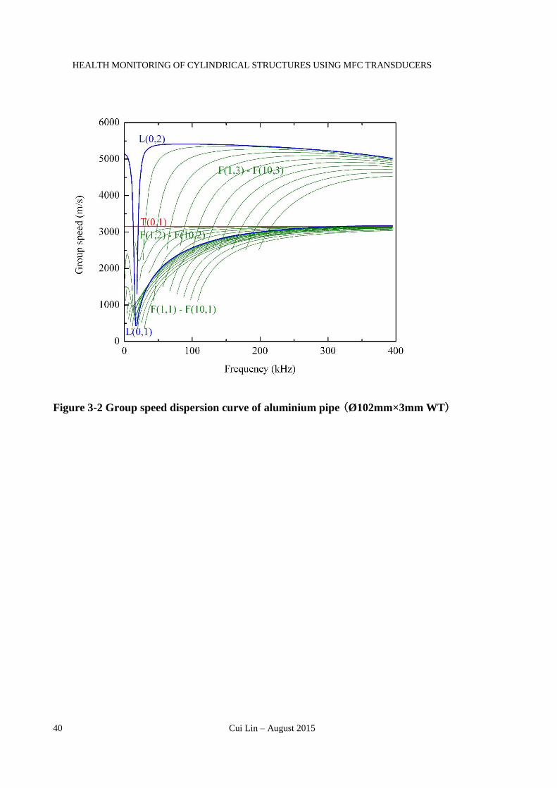
HEALTH MONITORING OF CYLINDRICAL STRUCTURES USING MFC TRANSDUCERS
40 Cui Lin – August 2015
Figure 3-2 Group speed dispersion curve of aluminium pipe (Ø102mm×3mm WT)

Chapter 3: Axial Crack Growth Monitoring of Cylindrical Structure
Cui Lin – August 2015 41
Figure 3-1 and Figure 3-2 listed the first 10 orders of flexural wave that corresponding
to axisymmetric wave modes L(0,1), T(0,1) and L(0,2).The red lines in both Figure 3-1
and Figure 3-2 represent the axisymmetric wave mode T(0,1), which is a non-dispersion
wave with fixed wave speed. The two blue lines denote the other two axisymmetric
wave modes in the given frequency range: the first order longitudinal wave mode L(0,1)
and the second order longitudinal wave mode L(0,2). The three types of axisymmetric
wave are the most fundamental and common waves existing in cylindrical structures.
The following number in the bracelet represents the family number of either torsional
waves or longitudinal waves. There is no 2nd order torsional waves or 3rd order
longitudinal waves showed in Figure 3-1 and Figure 3-2. This is because with given
targeting frequency range (0-400 kHz) and testing material (aluminium pipe
Ø102mm×3mm WT), the cut-off frequency of those high order axisymmetric waves is
greater than the upper limit of the given frequency range, which is 400 kHz, those wave
modes cannot be activated. Those green color lines represent flexural wave modes
F(m,n). Those flexural wave modes are non-axisymmetric wave modes. At any given
cross section that perpendicular to the axis of the pipe, non-axisymmetric wave modes
do not share same displacement value on the circumference. Table 3-1 listed the group
speed of axisymmetric wave modes and non-axisymmetric wave modes. Take L(0,2)
and F(m,3) for example, at 100 kHz, L(0,2)’s group speed is 5412 m/s and F(5,3)’s
group speed is 2438 m/s. The difference is almost 3000m/s. However, at 250 kHz,
L(0,2)’s group speed is 5282 m/s and F(5,3)’s group speed is 4990 m/s. The difference
is almost 292m/s. This phenomenon can be explained as: with the same wave family
number n, flexural waves F(m,n) (m = 1…n) share similar wave speed as their
corresponding axisymmetric wave mode when the frequency is going towards the
higher end.

HEALTH MONITORING OF CYLINDRICAL STRUCTURES USING MFC TRANSDUCERS
42 Cui Lin – August 2015
Table 3-1 lists the group speed of an aluminium pipe with 103mm diameter and 3mm
wall thickness; the actuation frequency is 100 kHz, 150 kHz, and 250 kHz, respectively.
The blank slots mean these wave modes cannot be activated since the actuation
frequency is below cut-off frequency. The wave structures of each flexural wave modes
can be calculated based on the governing equation (Rose 1999). Figure 3-3 shows the
first three order of waves with the same family number but different circumferential
order. When circumferential order m is small, the wave structures of flexural waves are
quite similar to the wave structures of the corresponding axisymmetric wave modes.
However, when the circumferential order goes up, wave structure and amplitude will
become more and more complex, and it will increase the difficulty of interpretation of
output signals. Since axisymmetric waves have the same value at anywhere on the
circumference of the pipe, the axisymmetric waves usually compose the main structure
of the output signal, and they are easier to be detected and identified.
Figure 3-3 Circumferential order of flexural waves (m = 0~3)

Chapter 3: Axial Crack Growth Monitoring of Cylindrical Structure
Cui Lin – August 2015 43
Table 3-1 Group speed of different wave modes at 100 kHz, 150 kHz, and 250 kHz
actuation (m/s)
Wave
Mode 100 kHz 150 kHz 250 kHz
L(0,1) 2570 2869 3109
F(1,1) 2567 2867 3108
F(2,1) 2559 2861 3105
F(3,1) 2545 2851 3100
F(4,1) 2526 2837 3092
F(5,1) 2500 2819 3082
F(6,1) 2468 2797 3070
F(7,1) 2429 2770 3056
F(8,1) 2381 2738 3040
F(9,1) 2326 2702 3021
F(10,1) 2261 2661 3000
T(0,1) 3149 3149 3149
F(1,2) 3131 3142 314
F(2,2) 3076 3120 3140
F(3,2) 2984 3084 3128
F(4,2) 2855 3033 3111
F(5,2) 2685 2966 3090
F(6,2) 2470 2883 3064
F(7,2) 2196 2783 3032
F(8,2) 1834 2664 2996
F(9,2) 1296 2524 2954
F(10,2) - 2358 2907
L(0,2) 5412 5389 5282
F(1,3) 5324 5353 5271

HEALTH MONITORING OF CYLINDRICAL STRUCTURES USING MFC TRANSDUCERS
44 Cui Lin – August 2015
Wave
Mode 100 kHz 150 kHz 250 kHz
F(2,3) 5052 5246 5236
F(3,3) 4561 5061 5179
F(4,3) 3770 4789 5097
F(5,3) 2438 4416 4990
F(6,3) - 3914 4855
F(7,3) - 3226 4692
F(8,3) - - 4496
F(9,3) - - 4263
F(10,3) - - 3987
3.1.2 Conventional Damage Detection for Tubular Structures
Conventional damage detection is usually on a pulse-echo basis (Ditri and Rose 1992,
Ditri and Rose 1993, Li and Rose 2001, Demma et al. 2003, Sun et al. 2003, Sun et al.
2005b, Kannan et al. 2007, Rose et al. 2009). The actuators are usually needed to cover
the pipe circumference fully, or actuators need to be symmetrically distributed around
the circumference of the pipe so as to generate the axisymmetric target wave mode.
Otherwise, flexural wave modes will disturb the axisymmetric wave modes and will
interfere the reading.
Another shortage of traditional damage detection method for tubular structures is the
actuators are usually placed at one free end of host structure to eliminate the boundary
reflections which will also disturb the reading. Such arrangement limited the application
to be used on continuous pipelines, and almost impossible to be integrated into a system
to achieve automatical damage detection.
3.1.3 Crack Types on Cylindrical Structures
Circumferential direction cracks are sensitive to most of the waves that propagate in
cylindrical structures since the crack orientation is perpendicular to the wave
propagation direction. As shown in Figure 3-3, no matter for which type of waves,

Chapter 3: Axial Crack Growth Monitoring of Cylindrical Structure
Cui Lin – August 2015 45
axisymmetric wave modes or non-axisymmetric wave modes, continuous circumference
is one of the necessary boundary conditions to ensure the wave propagate smoothly.
When such continuity is broken, disturbance at the discontinuity will happen and affect
the output. The larger the discontinuity is, the greater disturbed output signal it can be
expected. However, cracks in pressure vessels and pipelines are most likely to occur
along its axial direction instead of the circumferential direction because of the higher
hoop stress. Since the particle motion direction of longitudinal wave modes L(0,n) is
parallel to the wave propagation direction, the sensitivity of L(0,n) is significantly
reduced for the axial direction crack. Compared to the longitudinal wave, torsional
wave’s particle motions are perpendicular to the wave propagation direction. The
propagation of torsional wave pack is disturbed and interrupted by the axial direction
crack. The disturbances in torsional wave pack are picked up by the sensors. Crack size
growth monitoring is thus achieved through the analysis of the changes of torsional
wave pack due to cracks, which is the basis of this chapter.
3.2 Method of Study
The aim of this section is to develop an axial crack detection and monitoring scheme for
the cylindrical structure using torsional wave. Unlike longitudinal wave, whose particle
motion is parallel to the axial crack orientation, torsional wave’s particle motion is
perpendicular to the axial crack. So torsional wave is expected to be easily affected by
axial direction crack on cylindrical structures.
Conventional damage detection method for tubular structures usually required the
actuators to cover the circumference of the pipe entirely to generate guided waves, the
advantage of such arrangement is with actuators covered most of the circumference, the
axisymmetric wave is easily generated. However, such arrangement also has shortages.
The conventional testing method usually requires the actuators and sensors be placed at
one end of the pipe. The reason to do so is that such arrangement can avoid the
reflection from one free end, so the echo signal from crack and echo signal from another
open end will be identified based on pulse-echo method. The position of crack can also
be located. However, such arrangement also required the testing structure must have an
open end, and this is not achievable for monitoring of continuous cylindrical structures.
Furthermore, such arrangement usually has relatively complicated setup to drive the

HEALTH MONITORING OF CYLINDRICAL STRUCTURES USING MFC TRANSDUCERS
46 Cui Lin – August 2015
probes to generate guided waves and retrieve data from the testing specimen. Such
experiment system is not easy to be moved or relocated due to the complicated setup
which also limited its industrial application. To overcome the shortages of conventional
damage detection method for cylindrical structures, MFC is proposed to be used as
actuators and sensors. The highly flexible character of MFC made it easy to be curved
to suit the surface of the cylindrical pipe. The high actuation ability of MFC is used to
generate and collect surface waves in cylindrical structure. Unlike the conventional
actuation method, MFC actuator will not need to cover the whole circumference of the
pipe to generate/collect waves, the primary interest of the method used in this chapter is
to extract the useful information from the acquired signal which contained both
axisymmetric wave modes and non-axisymmetric wave mode. Additionally to the
benefits mentioned earlier, in the method used in this chapter the actuator and sensor are
placed at both sides of the crack. This setup is used to monitor the occurrence of the
longitudinal crack and the growth of the longitudinal crack. The crack position detection
is not included in this chapter. The experiment setup used in this chapter can be further
developed and expanded for more applications like crack position identification and
crack orientation identification which will be discussed in Chapter 4 and Chapter 5,
respectively.
3.3 Numerical Simulation
3.3.1 Numerical Model of Specimen
To investigate the feasibility of axial crack detection and monitoring using torsional
wave, the FE simulation of guided wave propagation in a 1.2m long aluminium pipe
with 102mm diameter and 3mm wall thickness is performed using ANSYS, an FE
analysis software.
To simulate guided wave propagated in cylindrical structures, the numerical model must
be set up in ANSYS. ANSYS is a very powerful multi-physics analytical software. It
can solve both time domain and frequency domain problem.
The reason of using MFC in this experiment setup is when MFC is being actuated, due
to the bond between MFC and the host structure, the deformation of MFC will be
transferred to the surface of host structure to activate surface wave on host structure.
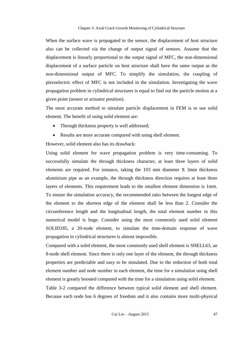
Chapter 3: Axial Crack Growth Monitoring of Cylindrical Structure
Cui Lin – August 2015 47
When the surface wave is propagated to the sensor, the displacement of host structure
also can be collected via the change of output signal of sensors. Assume that the
displacement is linearly proportional to the output signal of MFC, the non-dimensional
displacement of a surface particle on host structure shall have the same output as the
non-dimensional output of MFC. To simplify the simulation, the coupling of
piezoelectric effect of MFC is not included in the simulation. Investigating the wave
propagation problem in cylindrical structures is equal to find out the particle motion at a
given point (sensor or actuator position).
The most accurate method to simulate particle displacement in FEM is to use solid
element. The benefit of using solid element are:
Through thickness property is well addressed;
Results are more accurate compared with using shell element.
However, solid element also has its drawback:
Using solid element for wave propagation problem is very time-consuming. To
successfully simulate the through thickness character, at least three layers of solid
elements are required. For instance, taking the 103 mm diameter X 3mm thickness
aluminium pipe as an example, the through thickness direction requires at least three
layers of elements. This requirement leads to the smallest element dimension is 1mm.
To ensure the simulation accuracy, the recommended ratio between the longest edge of
the element to the shortest edge of the element shall be less than 2. Consider the
circumference length and the longitudinal length, the total element number in this
numerical model is huge. Consider using the most commonly used solid element
SOLID185, a 20-node element, to simulate the time-domain response of wave
propagation in cylindrical structures is almost impossible.
Compared with a solid element, the most commonly used shell element is SHELL63, an
8-node shell element. Since there is only one layer of the element, the through thickness
properties are predictable and easy to be simulated. Due to the reduction of both total
element number and node number in each element, the time for a simulation using shell
element is greatly boosted compared with the time for a simulation using solid element.
Table 3-2 compared the difference between typical solid element and shell element.
Because each node has 6 degrees of freedom and it also contains more multi-physical

HEALTH MONITORING OF CYLINDRICAL STRUCTURES USING MFC TRANSDUCERS
48 Cui Lin – August 2015
parameters, the total number of the equation to be solved in the solid element is much
greater than the total number of the equation to be solved in shell element.
Table 3-2 Comparison between typical shell element and solid element in ANSYS
Element Type Shell 63 Solid 186
No. of Node per element 8 20
No. of layers along thickness 1 3
No. of element along circumference 120 160
No. of element along longitudinal 480 1200
Total number of node 57.6×10³ 11.52×10⁶
Simulated time duration 300ms 300ms
Simulation time Around 5 minutes More than 24 hours
The penetrated axial direction crack at the centre of the pipe is modelled using nodal
release method, as shown in Figure 3-4. Node release method is a commonly used FE
method in crack propagation simulation. In an intact model, all nodes are connected to
the adjacent nodes. All the values of the parameters of this node are calculated based on
the nodes surrounding it. This node’s values will also be used to calculate the value of
its adjacent nodes. If this node is broke into two nodes at the same position but they are
not connected to each other, the values propagated to one node but cannot pass to the
other node, discontinuity occurred. Such discontinuity is considered to be a ‘crack.' If
more nodes on the line are broke into pairs, the ‘crack’ is considered growing. In
ANSYS model, two half shells are created in working space. The two half shells share
the same edges along the longitudinal direction. After meshing the shells, all nodes on
the shared edges can be grouped into pairs. Merge the nodes that share the same
coordinate in working space will create an undamaged cylinder. As shown in Figure 3-4,
at the centre of one shared edge of the two half shells, 7 group of nodes are highlighted.
Those nodes are selected to simulate the longitudinal direction crack propagation. When
simulating the undamaged case, all the seven sets of nodes are merged as all the pairs of
nodes on the shared edges. Once the crack is generated, the DOF of node set 1 is
Chapter 3: Axial Crack Growth Monitoring of Cylindrical Structure
Cui Lin – August 2015 49
unmerged. As the crack is gradually growing, more sets of nodes are unmerged. The
merged pairs of nodes are released to prevent physical measurements transfer between
elements.
The fixed boundary condition is applied at one end of the pipe to prevent rigid body
movement.
Figure 3-4 FE model of aluminium pipe with crack propagation (using nodal
release method)

HEALTH MONITORING OF CYLINDRICAL STRUCTURES USING MFC TRANSDUCERS
50 Cui Lin – August 2015
3.3.2 Actuators and Sensors Modelling
Unlike in the pulse-echo method, the crack existence is identified from additional wave
pack reflected from the crack. In the proposed method, the transducers are placed at
both sides of the crack. The presence of the crack is identified based on the analysis of
the change of the first pass-by wave packs.
The wave propagation paths and transducer distribution are depicted in Figure 3-5. As
shown in Figure 3-5, the actuator to sensor distance of 550 mm is used. All wave packs
will start from the actuator and propagate along the pipe; the wave pack will pass-by the
crack and finally reached the sensor position. Based on the group dispersion speed
differences( taking 100 kHz actuation as an example), the predicted arrival time of each
wave pack is listed in Table 3-3, only the first three circumferential orders of flexural
waves modes are listed.
Table 3-3 Predicted wave pack travelling time-based on group speed dispersion
curve (only the first three circumferential order are considered n=0~3)
Wave Mode Path 1 (s) Path 2 (s) Path 3 (s)
L(0,1) 214.0 470.8 463.0
F(1,1) 214.3 471.4 463.6
F(2,1) 214.9 472.8 465.0
F(3,1) 216.1 475.4 467.6
T(0,1) 174.7 384.2 377.9
F(1,2) 175.7 386.5 380.1
F(2,2) 178.8 393.4 386.9
F(3,2) 184.3 405.5 398.8
L(0,2) 101.6 223.6 219.9
F(1,3) 103.3 227.3 233.5
F(2,3) 108.9 239.5 235.6
F(3,3) 120.6 265.3 260.9

Chapter 3: Axial Crack Growth Monitoring of Cylindrical Structure
Cui Lin – August 2015 51
Figure 3-5 (a) Wave propagation paths; (b) Simplification of full actuation; (c)
Simplification of partial actuation; (d) actual MFC transducers on pipe
Actuator Sensor
(d)

HEALTH MONITORING OF CYLINDRICAL STRUCTURES USING MFC TRANSDUCERS
52 Cui Lin – August 2015
The model of transducers is simplified in the numerical model. The piezoelectric
characteristic of MFC is not considered in the simulation. In the proposed setup, MFC is
45˚ oriented against the pipe central axis, as both actuator and sensor. This arrangement
is because the deformation of MFC along its long axis can be projected into two
directions, pipe axial direction and pipe circumferential direction. The axial direction
actuation will generate longitudinal wave packs; the circumferential direction actuation
will generate torsional wave packs.
Two types of simulation are considered in the simulation, full actuation and partial
actuation. Full actuation condition considered the actuator covered the entire
circumference of tubular structure, axial and circumferential force conditions are
applied to all the nodes on the circumference at actuator position as shown in Figure
3-5(b), where only the axisymmetric wave modes T(0,n) and L(0,n) are activated. Such
arrangement is the ideal case where only axisymmetric wave modes are activated which
is not feasible to achieve when using MFC as actuators. According to the proposed
experimental setup, where MFC can only cover partial of the circumference of the pipe,
the axial and circumferential force boundary conditions are also covered the only partial
of the circumference, as showed in Figure 3-5 (c). In actual condition, MFC covers an
area which has both longitudinal dimension and circumferential dimension. Due to
simplification, the numerical simulation of partial actuation condition only consider the
nodes at actuator position on the circumference are being activated. Since partial
actuation condition only activates part of the circumference, the flexural wave modes
are activated.
3.3.3 Actuation Signal
5-cycles Hanning windowed sinusoidal wave tone burst was used as the actuation signal.
The Hanning window function is expressed in Eq. 3-1. If the 5-cycles sinusoidal tone
burst has a frequency f, then the TH equals to the number of counts times the period of
this burst.
𝐻(𝑡) =1
2[1 − 𝑐𝑜𝑠 (
2𝜋𝑡
𝑇𝐻)] Eq. 3-1
The 5-cycles Hanning windowed sine wave is compared with normal 5-cycles sine
wave burst in Figure 3-6, both signals are being actuated at 100 kHz frequency.

Chapter 3: Axial Crack Growth Monitoring of Cylindrical Structure
Cui Lin – August 2015 53
Figure 3-6 Comparison of actuation signals: Hanning windowed sine wave, and
original sine wave burst at 100 kHz actuation frequency

HEALTH MONITORING OF CYLINDRICAL STRUCTURES USING MFC TRANSDUCERS
54 Cui Lin – August 2015
Compared with normal 5-cycles sine wave burst, the Hanning windowed sine wave
burst have a ‘centred’ middle peak. This feature of signal make the post-processing of
output signal easier: the targeting wave pack is easy to be located when it has a centred
peak.
Another reason of using Hanning window to filter the original sine wave tone burst is to
get a relatively purified actuation signal with concentrated frequency bandwidth. Figure
3-7 compares the Fast Fourier Transform (FFT) of the two actuation signals: Hanning
windowed 5-cycles sine wave and normal 5-cycles sine wave tone burst. Fourier
analysis converts the signal from time domain to frequency domain to demonstrate its
frequency character. From Figure 3-7, it can be found that when being activated at 100
kHz, the normal 5-cycles sine wave tone burst has more frequency components in the
frequency domain. Since guided waves have dispersion character, the wave packs will
become dispersed during propagation. More frequency components will generate more
waves at different propagation speed, which will greatly interfere the main wave pack
and cause trouble to the interpretation of output signal. After filtering by Hanning
window, the sine wave burst has concentrated frequency bandwidth in the frequency
domain which reduced the complexity of dispersion behaviour and extrusive centre
peak in the time domain.

Chapter 3: Axial Crack Growth Monitoring of Cylindrical Structure
Cui Lin – August 2015 55
Figure 3-7 Fast Fourier Transform of Hanning windowed sine wave and normal
sine wave tone burst

HEALTH MONITORING OF CYLINDRICAL STRUCTURES USING MFC TRANSDUCERS
56 Cui Lin – August 2015
3.3.4 Actuation Frequency
100 kHz frequency has been chosen as actuation frequency. This specific actuation
frequency 100 kHz is chosen based on several facts.
Towards the high-frequency end:
(1) The element size.
To ensure the element can capture the accurate response of specimen, the
element size is suggested to be around 1/10th of the wavelength. The higher the
actuation frequency is used, the narrower the wave pack will be and the less
interference will happen between wave packs. However, on the other hand, the
higher the actuation frequency it is, the shorter the wavelength will be, and the
denser mesh will be required to secure the simulation accuracy which will
double reduce the efficiency of the simulation.
(2) The experiment equipment limitation
Even though regardless of simulation time, a numerical simulation can achieve
higher actuation frequency as possible. However, in practise, the actuation
frequency also depends on the limit of experiment equipment. The arbitrary
function generator usually has a bandwidth limitation. The signal amplifier
which is connected to the function generator also has bandwidth limitation. Most
of the time, when the actuation signal is beyond the upper limit of the equipment,
the equipment capacity is greatly dropped. The amplified signal quality will
greatly drop and the noise-to-signal ratio will increase. Those facts will lead to
the inaccuracy of the interpretation of the experimental data. Equipment
limitation usually limits the actuation frequency within 200 kHz.
Towards the low frequency end:
A lower frequency will take more time to generate the signal. Take five cycles
Hanning windowed sine wave at 60 kHz for example; it will take 83 s (10-6
second) to complete the generation of the signal. Assume the Actuator-to-Sensor
distance is 0.55m; at 60kHz, as per the group speed dispersion curve, both
torsional wave speed and longitudinal wave speed are quite similar to the
corresponding wave speed at 100 kHz actuation frequency. Assume that the
wave speeds differences can be neglected, then all wave packs will arrive at the

Chapter 3: Axial Crack Growth Monitoring of Cylindrical Structure
Cui Lin – August 2015 57
same position as compared with 100 kHz actuation signal used case. Figure 3-8
shows the wave shape of sensor output at 100 kHz. In Figure 3-8, the torsional
wave pack is separated with longitudinal wave pack. If the actuation signal is
changing from 100 kHz actuation frequency to 60 kHz actuation frequency, each
wave pack will increase 60% of its original width. Then the torsional wave pack
will be overlapped with longitudinal wave pack. Hence for this particular testing
specimen, 100 kHz auction frequency is better than 60 kHz auction frequency.
However, 60 kHz actuation frequency is also suitable for the experiment if the
testing specimen have a longer actuator to sensor distance to separate the
torsional wave pack and longitudinal wave pack.
Take all the three aspects into consideration, 100 kHz actuation frequency is chosen to
make sure all points are well addressed. Unless noted otherwise, all actuation frequency
used in this dissertation is fixed at 100 kHz.
To be noted, the selection of actuation frequency relies on trial and error. There is no
fixed frequency for the testing, as long as the actuator successfully activates the target
wave modes and the sensor is acquiring useful information that can be used for crack
identification, the actuation signal frequency is suitable to be employed.
3.3.5 Full Actuation Simulation of Guided-Wave Propagating in Tubular
Structure
Purely full actuation of guided waves in the cylindrical structure is only achievable in
numerical simulation. When actuators have fully covered the circumference of the
tubular and worked simultaneously, only the axisymmetric wave modes are activated.
Extract the output of the node at the sensor location, the simulation results of full
actuation case of the undamaged specimen and damaged specimen (with 40mm axial
oriented crack) are plotted in Figure 3-8. Output results amplitude are normalized
against the magnitude of the actuation signal to give a better demonstration. Assume the
actuation signal have unit amplitude, the output signal amplitude is non-dimensional
after divided by the maximum actuation signal. Below points can be found in Figure 3-8:
Outputs from both undamaged case and damaged case have three significant
wave packs.
There is no significant time of flight (TOF) difference between the two outputs.

HEALTH MONITORING OF CYLINDRICAL STRUCTURES USING MFC TRANSDUCERS
58 Cui Lin – August 2015
Compared with the undamaged case, the first wave pack of damaged case has
amplitude changed barely; the second wave pack of damaged case has obvious
amplitude change compared with the amplitude change of the first wave pack.
The magnitude of the third wave pack also doesn’t change much.
The first and third wave packs from damaged case matched the wave packs from
undamaged case quite well. The second wave pack from damaged case appears
‘wider’ compared with wave pack from the undamaged case. The difference
comes from the crack.
The wave speeds of first two wave packs are calculated from the TOF of the wave pack
(center-to-center) and the actuator-to-sensor distance. Compared with the wave speed
listed in Table 3-1, the calculated wave pack speeds of the first and second wave packs
are well matched with group speeds of symmetric wave modes L(0,2) and T(0,1),
respectively. The maximum deviation from the theoretical result is around 3%. The
calculation results are listed in Table 3-4.
From Figure 3-8, it can be concluded that the axially oriented crack has a greater impact
on passed-by torsional wave mode, but it has barely effect on longitudinal wave mode.

Chapter 3: Axial Crack Growth Monitoring of Cylindrical Structure
Cui Lin – August 2015 59
Table 3-4 Simulation results wave packs group speed calculation
Wave
pack
C-to-C
TOF(mS)
A-to-S
Distance
(mm)
Calculated
Group Speed
(m/s)
Theoretical
Group Speed
(m/s) Difference
1st 104 550 5288.5 5412 2.29%
2nd 180 550 3055.6 3149 2.97%
Figure 3-8 Comparison of full actuation outputs from undamaged case and
damaged case

HEALTH MONITORING OF CYLINDRICAL STRUCTURES USING MFC TRANSDUCERS
60 Cui Lin – August 2015
Even though the existence of the axially oriented crack changes the torsional wave
pack’s amplitude and overall wave shape, the changes of the signal are tiny, and they
are hard to trace in a quantitative way. Numerical simulations of the damaged case start
from 2.5mm crack (Release one node) until crack size reached 42.5mm (release 17
nodes). The pitch-catch method is one of the commonly used ways to trace the change
of signal amplitude. However, it cannot produce a recognizable pattern between the
peak value changes of each wave pack and the growing crack size. In Figure 3-8, the
two ‘expected’ maximum changes of torsional wave pack amplitude are marked as point
A and point B, which are the maximum and minimum amplitude of the targeting wave
pack. Figure 3-9 plots the absolute values of both point A and point B. Each data point
represents either point A or Point B amplitude from corresponding simulation results.
As it can be found in Figure 3-9, there is no clear pattern can be found when crack size
is growing larger and larger. No firm conclusion can be drawn from the result of pitch-
catch method. Even though the results from point B demonstrated a ‘trend’ of growing
pattern along with the growing crack, the absolute normalized amplitude change is less
than 10-6 of the absolute peak amplitude. This value of change is too weak to be used as
an indicator of crack changes. Other more efficient and easy to recognized method shall
be used to reflect the crack size growth.

Chapter 3: Axial Crack Growth Monitoring of Cylindrical Structure
Cui Lin – August 2015 61
Figure 3-9 Absolute amplitude change of Point A and Point B from numerical
simulation of undamaged and damaged cases

HEALTH MONITORING OF CYLINDRICAL STRUCTURES USING MFC TRANSDUCERS
62 Cui Lin – August 2015
3.3.5.1 Root Mean Square Deviation Crack Index
Root mean square deviation (RMSD), which is defined as
𝑅𝑀𝑆𝐷 = √∑ (𝑥𝑖−𝑥0)2𝑛
𝑖=1
∑ 𝑥02𝑛
𝑖=1
× 100 Eq. 3-2
is a commonly used method to evaluate the difference between a new set signal and the
original signal. Assume that there is axially oriented crack exists on the tubular structure.
Due to wave mode particle motion direction, the crack is sensitive to torsional wave
pack and it is not sensitive to longitudinal wave pack. It could be expected that the
torsional wave pack will be more distorted if the wave pack passed the crack.
Meanwhile, longitudinal wave pack will not be affected as much as torsional wave pack.
If the actuation wave pack length is known, based on the wave mode group speed
dispersion curve, the targeted longitudinal wave pack, and torsional wave pack can be
identified. RMSD method is used to measure how much difference between the signals
collected from cracked specimen and the original signals. As the crack growth, the
torsional wave pack will be distorted more and more, and the change of wave pack will
be reflected on the RMSD value change, and the longitudinal wave will remain the
original shape where the RMSD value changes are quite small.
A modified equation based on Eq. 3-2 is used here to evaluate the total change of the
targeting wave pack as
𝑅𝑀𝑆𝐷𝑝𝑖 (𝑡) = √
∑ [𝑥𝑖(𝑡)−𝑥0(𝑡)]2𝑡0+𝑡𝑎𝑡0
∑ 𝑥02(𝑡)
𝑡0+𝑡𝑎𝑡0
× 100 Eq.3-3
where t0 is the starting point of the time interval and ta is the actuation signal length.
From t0 to ta defines the time window to calculate the deviation. Take 100 kHz actuation
for example; the actuation signal is a 5-cycles Hanning windowed sine wave tone burst.
The duration of this actuation signal is 50ms. So a 50ms long time window will be used
to select targeting signal that is used to calculate the deviation. Assume there is no
dispersion happened after the wave pack travelled for a certain while, the wave pack
shape is unchanged. However, if there are discontinuous on the wave propagation path,
the signal will be disturbed. Both crack tips will be functioned as a new wave source.
The wave interferes at crack tips. The original wave pack, as well as the two wave packs
from both end of crack tips, will travel together, and the output signal for the crack case

Chapter 3: Axial Crack Growth Monitoring of Cylindrical Structure
Cui Lin – August 2015 63
will be different from the undamaged case. The 𝑅𝑀𝑆𝐷𝑝𝑖 (𝑡) value calculates the
disturbance on wave pack p that starts at t0 with duration of ta. The superscript i
represents the data xi(t) comes from the ith experiment( with i×2.5mm crack size). The
value 𝑅𝑀𝑆𝐷𝑝𝑖 (𝑡) is used to quantify the disturbance caused by the axial oriented crack
and to establish the relationship between crack size and the output signals. Figure 3-10
demonstrated the 50ms long time window to calculate the RMSD value of 2nd order
longitudinal wave pack L(0,2) and the RMSD value of 1st order torsional wave pack
T(0,1) in blue and red dash line windows, respectively. In Figure 3-10, only damaged
case with 40mm axial oriented crack is compared with undamaged case. Take all the
RMSD value calculated from simulation case 1 to case 17 and plot them against the
crack size growth in Figure 3-11.
Figure 3-10 Time window for second order longitudinal wave pack L(0,2) and first
order torsional wave pack T(0,1)
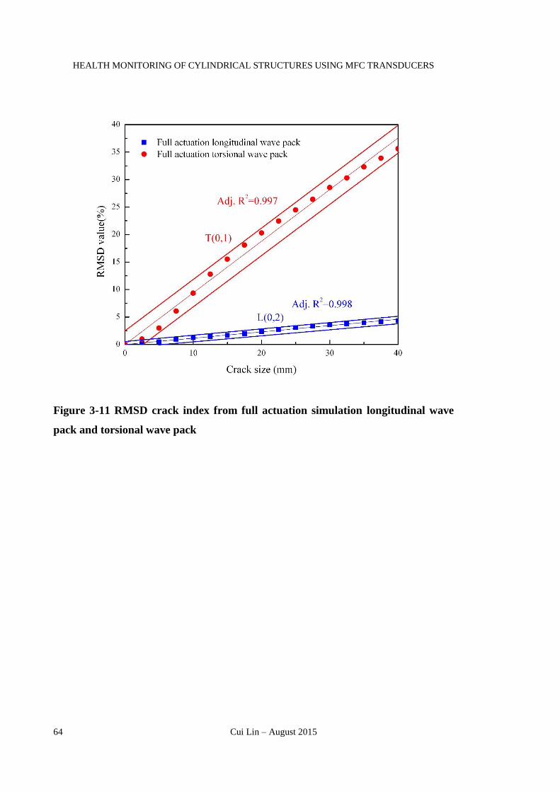
HEALTH MONITORING OF CYLINDRICAL STRUCTURES USING MFC TRANSDUCERS
64 Cui Lin – August 2015
Figure 3-11 RMSD crack index from full actuation simulation longitudinal wave
pack and torsional wave pack
Chapter 3: Axial Crack Growth Monitoring of Cylindrical Structure
Cui Lin – August 2015 65
As shown in Figure 3-11, the RMSD values from both second order longitudinal wave
pack and first order torsional wave pack demonstrate a linear growth relationship
against the axial direction crack growth with R2 almost equal to 1. R2 is an indicator of
the quality of linear regression. The closer between R2 and 1, the better the linear
regression quality it is, which means the data are better fitted on a line.
Since in longitudinal wave mode, all the particles vibrate along the axis of tubular, the
axial direction crack will not have a significant effect on the particle motions of
longitudinal wave packs. Compared with longitudinal wave packs, in torsional wave
packs, the particle vibrate in the circumferential direction. The axially oriented crack
caused discontinuity on the propagation paths of torsional wave pack. Hence, even
though both wave packs showed a linear relationship between the RMSD value and the
growing crack size, the RMSD values calculated from torsional wave pack demonstrates
a steeper slope compared with the RMSD value calculated from longitudinal wave pack.
This result indicates that the torsional wave pack is more sensitive than longitudinal
wave pack on axially oriented crack, which is exactly as we have mentioned in the
previous section.
3.3.6 Partial Actuation Simulation
Full simulation condition can only be achieved in numerical simulation. In actual
application, due to the limitation of the actuator, only part of the tubular circumference
can be driven. Partial actuation will lead to the generation of flexural wave modes
F(m,n), which will have dispersion effect during wave propagation. The wave
dispersion effect will interfere the interpretation of output signal, which is not good for
the RMSD crack index.
To compare the simulation results with experiment results, partial actuation cases are
also studied in numerical simulation.
In partial actuation numerical simulation, only part of the nodes on the circumference at
actuator positions have been activated. Consider the MFC functional area and it is 45
degree oriented on the pipe, around 40 degrees of the circumference is activated as
shown in Figure 3-5. Since only partial of the circumference is activated, the flexural
wave modes are activated together with the axisymmetric wave modes, as illustrated in
Figure 3-12.

HEALTH MONITORING OF CYLINDRICAL STRUCTURES USING MFC TRANSDUCERS
66 Cui Lin – August 2015
Figure 3-12 Comparison of partial actuation simulation results between damaged
and undamaged cases

Chapter 3: Axial Crack Growth Monitoring of Cylindrical Structure
Cui Lin – August 2015 67
Figure 3-12 compared the output from partial actuation undamaged case and damaged
case. In the damaged case simulation, the 40mm axial oriented crack case is used. The
reason to compare the 40mm cracked case with the undamaged case is to demonstrate
the maximum output signal difference between undamaged and damaged cases. Similar
to the finding from full actuation simulation output, even though the damaged case has a
very long axial direction crack already, from Figure 3-12 it is also impossible to get the
signal amplitude change via pitch-catch method. Take the torsional wave pack for
instance; the five cycles tone burst have several peak amplitudes and some of the peak
value increases; some of them decreases; the rests are hard to tell whether they are
increased or decreased from the undamaged signal base.
The more the actuator covers the circumference of the pipe, the more dominant the
axisymmetric wave modes will be in the whole wave pack (Ditri and Rose 1992, Li and
Rose 2001). Figure 3-13 compares output signals from both full actuation and partial
actuation damaged case with 40mm crack. The induced flexural wave modes not only
changed the amplitude of wave packs but also changed the overall wave pack shape. In
full actuation case, two clearly separated wave packs belong to longitudinal wave mode
L(0,2) and torsional wave mode T(0,1), respectively. When flexural wave modes are
activated in partial actuation case, more wave packs are filled in between longitudinal
wave pack and torsional wave pack. These additional wave packs are flexural wave
packs.
To better demonstrate the overall wave shape change, Figure 3-14 compares the
envelope of the two output signals from full actuation and partial actuation. Compared
both output signals from full actuation and partial actuation case, below findings are
highlighted.
Compared with full actuation, each wave pack demonstrated dispersion effect.
The overall wave shape of partial actuation case is ‘wider’ compared with full
actuation case.
Flexural wave packs travel at similar but slower group speed compared with
their corresponding axisymmetric wave packs. The existence of flexural wave
packs will interfere the effect of axially oriented crack on torsional waves. In
partial actuation case, between longitudinal wave pack L(0,2) and torsional wave
pack T(0,1), there is one new wave pack from flexural wave modes F(m,n).
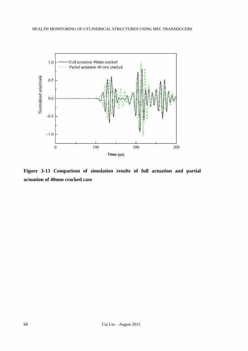
HEALTH MONITORING OF CYLINDRICAL STRUCTURES USING MFC TRANSDUCERS
68 Cui Lin – August 2015
Figure 3-13 Comparison of simulation results of full actuation and partial
actuation of 40mm cracked case
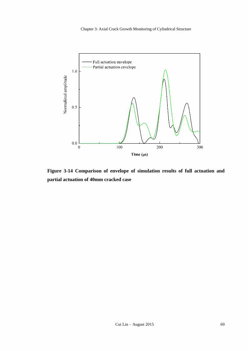
Chapter 3: Axial Crack Growth Monitoring of Cylindrical Structure
Cui Lin – August 2015 69
Figure 3-14 Comparison of envelope of simulation results of full actuation and
partial actuation of 40mm cracked case

HEALTH MONITORING OF CYLINDRICAL STRUCTURES USING MFC TRANSDUCERS
70 Cui Lin – August 2015
Flexural wave modes are also affected by the axially oriented crack, but due to
the particle movement direction of flexural wave mode is neither parallel to the
circumferential direction nor parallel to the longitudinal direction, the sensitivity
of flexural wave modes on axially oriented crack is expected to be in between
the sensitivity of torsional wave and sensitivity of longitudinal wave on the same
type of crack.
With the presences of flexural wave mode F(m,n), the output signal from partial
actuation is more complicated compared with full actuation output.
Taking all the partial actuation results into Eq. 3-3, an RMSD crack index for partial
actuation simulation results are plotted in Figure 3-15. Similar to Figure 3-11, Figure
3-15 shows the RMSD crack index calculated from the partial actuation simulation
result of two wave packs, torsional and longitudinal wave pack. Unlike full actuation
simulation results, in the RMSD crack index calculation, there is not only axisymmetric
wave modes but also non-axisymmetric wave modes. However, still, with the presence
of flexural wave modes in the computation of RMSD crack index, the effect of axial
direction crack is still more severe on torsional wave pack than that on longitudinal
wave pack. In partial actuation simulation, the torsional wave pack contains the
components of axisymmetric wave modes T(0,1) as well as its corresponding non-
axisymmetric flexural wave modes F(m,2); the first longitudinal wave pack contains the
component of axisymmetric wave modes L(0,2) and its corresponding non-
axisymmetric flexural wave modes F(m,3). The presence of flexural wave modes
lowered down the R2 value of the linear regression, which means the flexural wave
modes reduced the sensitivity of using torsional wave pack to monitor the axially
oriented crack growth.
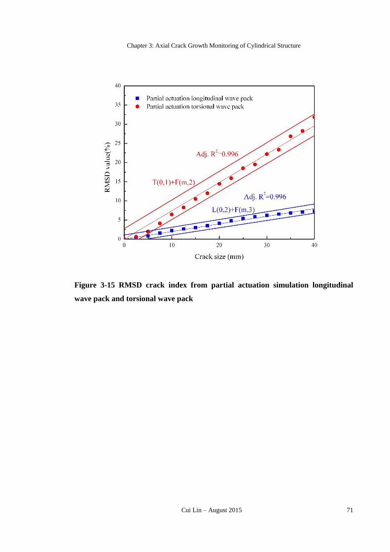
Chapter 3: Axial Crack Growth Monitoring of Cylindrical Structure
Cui Lin – August 2015 71
Figure 3-15 RMSD crack index from partial actuation simulation longitudinal
wave pack and torsional wave pack

HEALTH MONITORING OF CYLINDRICAL STRUCTURES USING MFC TRANSDUCERS
72 Cui Lin – August 2015
Figure 3-16 compares the RMSD crack index calculated from both full and partial
actuation. In the case of partial actuation, the ‘torsional’ wave pack also includes the
flexural wave modes F(m,2). Since the wave structures of flexural waves are only
partially affected by the axially oriented crack, when RMSD crack growth index is
calculated, the present of flexural waves F(m,2) reduce the sensitivity of crack growth
index as compared with the case of full actuation where only torsional wave, T(0,1), is
included. Similarly, the partial actuation caused “longitudinal” wave pack also includes
the flexural wave modes F(m,3) with is more sensitive to the axial crack than the L(0,2).
Therefore, the calculated RMSD crack growth index is better than for the case of full
actuation where only L(0,2) is included.
The foundation of this study is to use MFC generate axisymmetric wave modes
(torsional wave and longitudinal wave modes) in tubular structures to monitor the
structural healthy condition. In this section, partial actuation case is studied. Figure 3-13,
Figure 3-14 and Figure3-16 compare the full actuation results with the partial actuation
results. The comparison results show that when partial actuation method is used, more
flexural wave modes are activated. As explained in the previous section, when tubular
structure is fully activated, only axisymmetric wave modes can be activated. In partial
activation modes, flexural wave modes are also activated. In Figure 3-16, both crack
indexes generated using full actuation results and partial actuation results are compared.
Compared with full actuation torsional wave result and partial actuation torsional wave
result, the slope of the two curves is slightly different, where the data from full actuation
case is more sensitive to the crack growth than the data from partial actuation case. This
result reveals that when partial actuation case is used, the flexural wave modes F(m,n)
activated will interference with their corresponding axisymmetric wave modes T(0,n)
and L(0,n), hence reduced the sensitivity of the crack index.
Since the aim of this study is to use the axisymmetric for crack identification,
monitoring, and prediction, axisymmetric wave modes are the wave modes that are
functional. Hence to better represent the effectiveness of the proposed method, only full
actuation simulation results are used in following Chapters. However, to better compare
the experimental data and simulation results, more digital signal processing techniques
are required to extract the axisymmetric wave modes from the experimental data which
will be included in future studies.

Chapter 3: Axial Crack Growth Monitoring of Cylindrical Structure
Cui Lin – August 2015 73
Figure 3-16 Comparison of RMSD crack index between full actuation and partial
actuation simulation results
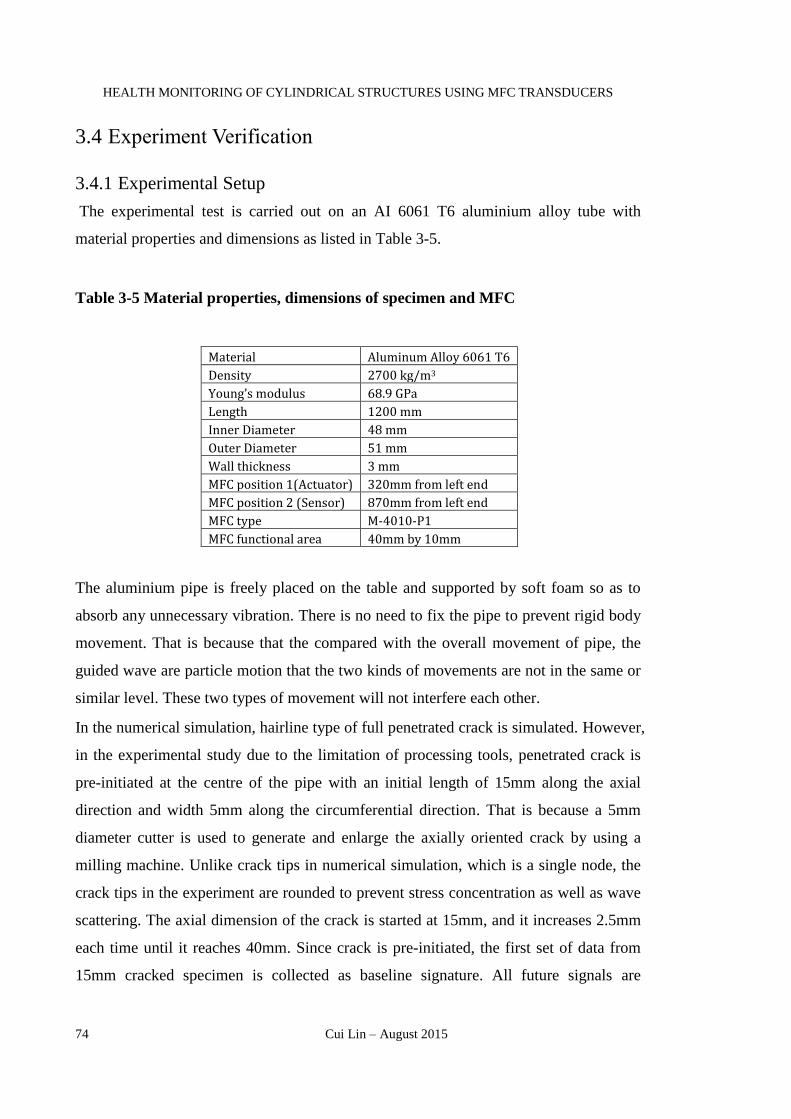
HEALTH MONITORING OF CYLINDRICAL STRUCTURES USING MFC TRANSDUCERS
74 Cui Lin – August 2015
3.4 Experiment Verification
3.4.1 Experimental Setup
The experimental test is carried out on an AI 6061 T6 aluminium alloy tube with
material properties and dimensions as listed in Table 3-5.
Table 3-5 Material properties, dimensions of specimen and MFC
Material Aluminum Alloy 6061 T6
Density 2700 kg/m3
Young’s modulus 68.9 GPa
Length 1200 mm
Inner Diameter 48 mm
Outer Diameter 51 mm
Wall thickness 3 mm
MFC position 1(Actuator) 320mm from left end
MFC position 2 (Sensor) 870mm from left end
MFC type M-4010-P1
MFC functional area 40mm by 10mm
The aluminium pipe is freely placed on the table and supported by soft foam so as to
absorb any unnecessary vibration. There is no need to fix the pipe to prevent rigid body
movement. That is because that the compared with the overall movement of pipe, the
guided wave are particle motion that the two kinds of movements are not in the same or
similar level. These two types of movement will not interfere each other.
In the numerical simulation, hairline type of full penetrated crack is simulated. However,
in the experimental study due to the limitation of processing tools, penetrated crack is
pre-initiated at the centre of the pipe with an initial length of 15mm along the axial
direction and width 5mm along the circumferential direction. That is because a 5mm
diameter cutter is used to generate and enlarge the axially oriented crack by using a
milling machine. Unlike crack tips in numerical simulation, which is a single node, the
crack tips in the experiment are rounded to prevent stress concentration as well as wave
scattering. The axial dimension of the crack is started at 15mm, and it increases 2.5mm
each time until it reaches 40mm. Since crack is pre-initiated, the first set of data from
15mm cracked specimen is collected as baseline signature. All future signals are

Chapter 3: Axial Crack Growth Monitoring of Cylindrical Structure
Cui Lin – August 2015 75
compared with the baseline signature, and they are used to generate the RMSD crack
index.
The conventional PZT transducers have the weakness of being too brittle to be attached
to the nonplanar surface. Hence, flexible MFC transducer is used as both actuator and
sensor in this study. Compared with a typical through-plane poled PZT actuator, the
maximum free strain performance of MFC is considerably larger and is also very
durable under various electrical and mechanical cyclic loading conditions (W. Wilkie et
al. 2002). Because of its manufacturing process and its structure, MFC shows different
electromechanical characteristic along its long and short edges. For simplicity, only the
dominant strain along its long edge is used in this experiment. MFC transducers M-
4010-P1 with functional area 40 mm by 10 mm are bonded on the surface of the pipe,
45˚ oriented against the pipe central axis, as both actuator and sensor as shown in Figure
3-5(d) and Figure 3-17.
The experimental setup consists of a Tabor Electric ww5601 arbitrary function
generator, a TREK PZD350A high power amplifier and a National Instruments
integrated data acquisition (DAQ) system as shown in Figure 3-17. The 1-volt peak-to-
peak actuation signal from function generator is 100 times amplified before it is applied
to the MFC actuator. The MFC sensor is directly connected to the DAQ device to
receive the output signal. One additional cable from the function generator is connected
to the DAQ device to synchronize the actuation and DAQ process.
There is background white noise from alternating current (AC) which will contribute to
the deviation of the output signal. To eliminate such background white noise, 32-times
cycle averaging is used to reduce the influence of random noise. This function allowed
the DAQ device to collect 32 times data and stored temporarily in memory. Then the
average of the 32 times signal will be written to the output data file. The function
generator is setup to repeat the actuation signal every second. The 1-second interval
between two actuations is to make sure the guided waves generated from the previous
actuation is completely gone and newly generated guided wave will not be interfered by
last time generated waves.
As mentioned in Section 3.3.4, the actuation frequency cannot be neither too high nor
too low. When driven by signals with actuation frequency above 250 kHz, the actuation
ability of MFC is greatly depressed and the signal to noise ratio (SNR) is too low. On

HEALTH MONITORING OF CYLINDRICAL STRUCTURES USING MFC TRANSDUCERS
76 Cui Lin – August 2015
the other hand, under actuation frequency lower than 50 kHz, the wave packs are
overlapped with each other which increase the difficulty in extracting target wave pack
from the overall wave structure. Thus, only the actuation frequency of between 50 kHz
to 250 kHz is used in this research. To demonstrate the experiment results and
compared them with numerical simulation results, 100 kHz actuation frequency is
selected.
Figure 3-17 Experiment equipment setup

Chapter 3: Axial Crack Growth Monitoring of Cylindrical Structure
Cui Lin – August 2015 77
3.4.2 Signal Processing
Due to the limitation of DAQ device, the background AC noise cannot be fully removed
by just using the signal averaging technique. The original experimental results are
further processed before they can be utilized for calculating the RMSD crack growth
index.
The background AC noise has a fixed frequency of 50 Hz. So one full cycle of
background AC takes 0.02s. If guided wave is being activated at 1 kHz actuation
frequency, 5-cycle Hanning windowed sine wave tone burst takes 0.005S which is 1/4th
of the AC period. Figure 3-18 demonstrates how the AC background noise affects the
output signal. To remove the AC background noise, the exactly AC noise equation
must be found. It is known that the AC has fixed the period of T=0.02s, and the
amplitude of AC keep oscillating about the zero axes. Assume that the AC have below
expression
𝑓(𝑡) = 𝑎 ∗ 𝑠𝑖𝑛 [2𝜋(𝑡−𝑏)
𝑇] + 𝑐 Eq. 3-4
with T = 0.02 and c = 0, the sinusoidal curve f(t) for the background AC noise in the
experimental result is fitted by MATLAB curve fitting toolbox. Once a and b are
acquired, the AC background noise can be totally removed from the experiment results.
Figure 3-20 demonstrated the original experimental result and modified experimental
result using the method mentioned above as well as the fitted sine curve.

HEALTH MONITORING OF CYLINDRICAL STRUCTURES USING MFC TRANSDUCERS
78 Cui Lin – August 2015
Figure 3-18 Effect of AC background noise

Chapter 3: Axial Crack Growth Monitoring of Cylindrical Structure
Cui Lin – August 2015 79
Figure 3-19 Remove of AC background noise from experimental result

HEALTH MONITORING OF CYLINDRICAL STRUCTURES USING MFC TRANSDUCERS
80 Cui Lin – August 2015
3.4.3 Experimental Results
Since the aluminium pipe is pre-initiated with a 15mm long axial oriented crack, the
output signal collected from 15mm cracked specimen is being used as baseline structure
to calculate the RMSD crack index.
To compare the overall wave shape difference between full actuation numerical
simulation result, partial actuation numerical simulation result and experimental result,
normalization method is used to process the signals. Since RMSD method is to calculate
the deviation of two relevant data series, the normalization will not change the RMSD
crack index.
Figure 3-20 compares the three types of output signals mentioned above: full actuation
simulation result, partial actuation simulation result, and experimental result. In Figure
3-20. Compared with the full actuation simulation result, which only has axisymmetric
wave modes, both the partial actuation simulation result and the experimental results
include the non-axisymmetric flexural wave modes. The slight differences between the
partial actuation simulation result and experimental result are:
1) Some part of the amplitude of experimental results is greater than the partial
actuation simulation results;
2) At some part of the signal, the phase angle of these two signals cannot match.
These differences are caused by the simplification of actuator used during
simulation. As shown in Figure 3-5, in partial actuation simulation, all the force
boundary conditions have been applied on the circumference at the actuator’s centre
position and the output is also from a single node. On the other hand, in the
experiment, the actuator covers a particular area of the specimen where the output
from the sensor is an average of the total output of the MFC functional area. The
simplified transducers used in the simulation made the simulation results look
‘slimmer’ than the experimental results, as shown in Figure 3-20.
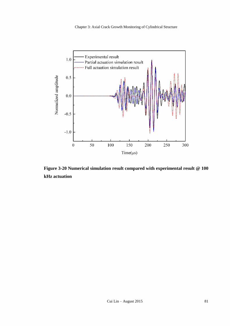
Chapter 3: Axial Crack Growth Monitoring of Cylindrical Structure
Cui Lin – August 2015 81
Figure 3-20 Numerical simulation result compared with experimental result @ 100
kHz actuation

HEALTH MONITORING OF CYLINDRICAL STRUCTURES USING MFC TRANSDUCERS
82 Cui Lin – August 2015
In both the partial actuation simulation result and the experimental result, the non-
dispersed torsional wave pack T(0,1) which is used to calculate the RMSD crack growth
index for axially oriented crack are mixed with the flexural wave modes; thus hard to
extract only T(0,1) wave pack. However, just as shown in Figure 3-16, even when
flexural wave modes are included in the targeting wave pack, the RMSD crack index for
axially oriented crack is still valid, just not as sensitive as using only pure torsional
wave pack. Taking the output from 15mm cracked case as baseline signature, the
RMSD crack growth index for axially oriented crack from the experimental results is
calculated and compared with those from the full actuation and partial simulation in
Figure 3-21.
Comparing the three RMSD crack growth indices obtained from the full actuation
simulation, partial actuation simulation and experimental result in Figure 3-21, the crack
growth index from numerical simulations suggests a very clear linear trend. In contrast,
the RMSD from the experimental result is slightly scattered. However, an
approximately linear relationship between the RMSD index and the crack size can still
be observed. There are several causes for the differences between these crack growth
indices:
1) The simplified actuator and sensor are modelling in numerical simulation.
In the numerical simulation, both actuating and sensing behaviour are simplified.
For activating, loading boundary conditions are added directly to the nodes
located at the actuator position on the circumference of tubular; for sensing, the
output from the node at sensor position on the circumference of tubular is used
as the output result. In both actuating and sensing case, the longitudinal direction
dimension of transducers is neglected. However, in the experiment, the
activating and sensing are achieved by using MFC. The MFC functional area
covers not only the circumference of the pipe but also the certain longitudinal
range of pipe, which will trigger more ‘dispersed’ flexural wave modes that will
interfere the RMSD crack index reading.
2) Simplified crack modelling in numerical simulation.
The crack model in numerical simulation is simplified as a pure hairline type of
crack with two shape crack tips. Circumferential direction dimension of crack is
not considered in the numerical simulation. However, in the experiment, the

Chapter 3: Axial Crack Growth Monitoring of Cylindrical Structure
Cui Lin – August 2015 83
minimum crack size can be achieved limited by the lab tools. The
circumferential direction dimension of crack is unneglectable. Reflection and
scattering will cause more dispersion behavior of flexural wave modes.
3) The bonding quality between MFC transducers to host structure.
The MFC transducers are connected to the host structure via super glue. The
bonding quality between MFC and the host structure will affect the testing result
very much. The actuation signal is transferred from MFC to host structure via
the epoxy layer at actuator position; the guided wave is also converted back to
electric signal via the bond between host structure and sensor.
4) Limitation of testing equipment
In the experimental test, the restriction of testing equipment will also contribute
to the quality of the signal collected. The noises from the laboratory background
and power supply need to be removed as much as possible which also lowered
the sensitivity of the proposed crack growth index.
5) The quality of testing results.
Last but not the least, the quality of the testing results is also important to the
final results. As shown in Figure 3-21, RMSD crack growth index from the
experimental result is more scattered compared with those from the numerical
simulation. Especially, at crack size 30mm and crack size 37.5mm, the deviation
looks much greater compared with other testing results. It can be expected that
the signal collected in such cases are ‘low quality’ signals. Since the crack on
the specimen is not reversible, to eliminate the effect of such ‘low quality’ signal,
it is suggested that for each case, at least three times output signals shall be
collected. If one of the signal quality is not good, the other two can be used to
replace the ‘bad’ signal that will deviate the final results.

HEALTH MONITORING OF CYLINDRICAL STRUCTURES USING MFC TRANSDUCERS
84 Cui Lin – August 2015
Figure 3-21 Comparison of RMSD crack growth index between full actuation,
partial actuation, and experimental result

Chapter 3: Axial Crack Growth Monitoring of Cylindrical Structure
Cui Lin – August 2015 85
3.4.4 Experiment Result and Discussion
Both numerical simulation and experimental results verified that using the above
calculated axial direction crack growth indices, the axially oriented crack growth can be
well monitored. From the numerical simulation results, it is easy to infer that if the
signal from the undamaged specimen is collected, this proposed method is capable of
detecting the crack at the incipient stage. From experimental results, it can be concluded
that if signals are collected at any given crack length, the crack propagation and failure
early warning can be achieved based on the RMSD crack growth index.
For the practical and economic reason, not all cracks on tubular structures are required
to be repaired when they are found. Only when the existing crack has
extended/accumulated to a critical level, the repair works it worth to be executed. Using
the proposed method in this chapter can help make the repair work more reasonable and
cost effective because a critical value of crack size can be pre-set in the crack growth
index. When the crack size matches the critical value, the crack must be repaired.
The background AC noise is harmful to the accuracy of the simulation. Isolated DAQ
device is suggested to be used in the data acquisition process. Otherwise, manual curve
fitting is needed to eliminate the background noise.
Since MFC transducers are used as both the actuator and sensor in this research and
they are placed on both side of the crack, a prototype of close-loop self-actuating and
sensing system for axial direction crack detection in continuous cylindrical structures is
proposed, as depicted in Figure 3-22. This system contains some transducers. For each
region, two pieces of transducer work together to monitor the health condition of this
region. For instance, region one monitoring will be performed by transducer 1 and 2. In
this sub-system, transducer one will be utilized as actuator and transducer two will be
utilized as a sensor. Once data has been collected, the system will switch scanning from
region 1 to region 2. In region 2, transducer two will be used as an actuator and the next
transducer will be utilized as a sensor. The system will control the area to be scanned,
and it will automatically switch the function of the transducers in the area as actuator
and sensor accordingly, and so forth so that the continuous pipe can be monitored.

HEALTH MONITORING OF CYLINDRICAL STRUCTURES USING MFC TRANSDUCERS
86 Cui Lin – August 2015
Figure 3-22 Prototype of a close-loop self-actuating and sensing axial direction
crack monitoring system for continuous cylindrical structures

Chapter 3: Axial Crack Growth Monitoring of Cylindrical Structure
Cui Lin – August 2015 87
3.5 Summary and Conclusion
This chapter presents a new proposed method that use torsional wave to measure and
monitor the propagation of axial direction crack in cylindrical structures. MFC is used
as both actuator and sensor because of its flexile character and strong actuating/sensing
capacity. MFC transducers are first applied to generate torsional wave for detecting and
monitoring axial direction crack growth in tubular structures. The actuator is driven by
pre-adjusted signals to produce target guided wave modes for inspection. The sensor
picks up the stress waves propagating in the pipe and returns the electrical signals. With
the help of digital signal processing (DSP) techniques, the damage information is
extracted from the changes of the sensor’s output. Both numerical and experimental
verifications have been conducted to demonstrate the effectiveness of this proposed
method. Based on the proposed method, a prototype of close-loop self-actuating and
sensing system for continuous cylindrical structures is proposed.
The results from the numerical simulation and experimental verification show that the
axial-direction crack propagation can be well monitored. The RMSD values of torsional
wave pack from a numerical simulation with different crack sizes give a linear trend
against the crack size increment. However, the numerical results do not match the
experimental results well. The difference is because the sensor and the actuator are
simplified in the numerical simulation, and the crack is also simplified using node
release method in which the crack width is not considered. Base on the analysis of both
numerical and experimental results, a linear relationship can be established between the
RMSD value of torsional wave pack and the axial direction crack size.
For the monitoring of continuous cylindrical structures, an integrated intelligent SHM
system is needed. The integration of crack orientation detection, crack location
identification, crack growth monitoring and optimized transducers distribution will be
discussed in following chapters.

HEALTH MONITORING OF CYLINDRICAL STRUCTURES USING MFC TRANSDUCERS
88 Cui Lin – August 2015
4 STRUCTURAL HEALTH
MONITORING SYSTEM FOR
AXIAL CRACK ON
CYLINDRICAL STRUCTURE
4.1 Introduction
In Chapter 3, a new proposed method that use torsional wave to measure and monitor
the propagation of axial direction crack in cylindrical structures has been proposed.
Based on the proposed method a close-loop self-actuating and sensing axial direction
crack monitoring system for continuous cylindrical structures has been proposed. With
the proposed monitoring system, the growth of axial direction crack can be well
monitored.
However, the proposed monitoring system has its limitation. Most of the time, the repair
work of damaged structure will require two fundamental information, ‘how severe the
damage is’ - whether it can be repaired or not; and ‘where the damage location is.' The
proposed monitoring system solved the first problem, the next problem of ‘where the
damage location is’ will be discussed in this chapter.
4.2 Method of Study
The aim of this section is to expand the method and SHM system developed in Chapter
3. The existing system developed in Chapter 3 can monitor the axially oriented crack
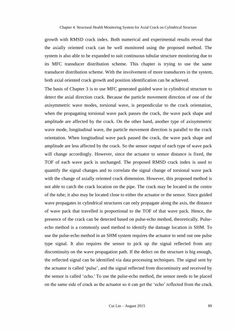
Chapter 4: Structural Health Monitoring System for Axial Crack on Cylindrical Structure
Cui Lin – August 2015 89
growth with RMSD crack index. Both numerical and experimental results reveal that
the axially oriented crack can be well monitored using the proposed method. The
system is also able to be expanded to suit continuous tubular structure monitoring due to
its MFC transducer distribution scheme. This chapter is trying to use the same
transducer distribution scheme. With the involvement of more transducers in the system,
both axial oriented crack growth and position identification can be achieved.
The basis of Chapter 3 is to use MFC generated guided wave in cylindrical structure to
detect the axial direction crack. Because the particle movement direction of one of the
axisymmetric wave modes, torsional wave, is perpendicular to the crack orientation,
when the propagating torsional wave pack passes the crack, the wave pack shape and
amplitude are affected by the crack. On the other hand, another type of axisymmetric
wave mode, longitudinal wave, the particle movement direction is parallel to the crack
orientation. When longitudinal wave pack passed the crack, the wave pack shape and
amplitude are less affected by the crack. So the sensor output of each type of wave pack
will change accordingly. However, since the actuator to sensor distance is fixed, the
TOF of each wave pack is unchanged. The proposed RMSD crack index is used to
quantify the signal changes and to correlate the signal change of torsional wave pack
with the change of axially oriented crack dimension. However, this proposed method is
not able to catch the crack location on the pipe. The crack may be located in the centre
of the tube; it also may be located close to either the actuator or the sensor. Since guided
wave propagates in cylindrical structures can only propagate along the axis, the distance
of wave pack that travelled is proportional to the TOF of that wave pack. Hence, the
presence of the crack can be detected based on pulse-echo method, theoretically. Pulse-
echo method is a commonly used method to identify the damage location in SHM. To
use the pulse-echo method in an SHM system requires the actuator to send out one pulse
type signal. It also requires the sensor to pick up the signal reflected from any
discontinuity on the wave propagation path. If the defect on the structure is big enough,
the reflected signal can be identified via data processing techniques. The signal sent by
the actuator is called ‘pulse’, and the signal reflected from discontinuity and received by
the sensor is called ‘echo.' To use the pulse-echo method, the sensor needs to be placed
on the same side of crack as the actuator so it can get the ‘echo’ reflected from the crack.
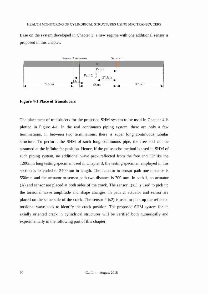
HEALTH MONITORING OF CYLINDRICAL STRUCTURES USING MFC TRANSDUCERS
90 Cui Lin – August 2015
Base on the system developed in Chapter 3, a new regime with one additional sensor is
proposed in this chapter.
Figure 4-1 Place of transducers
The placement of transducers for the proposed SHM system to be used in Chapter 4 is
plotted in Figure 4-1. In the real continuous piping system, there are only a few
terminations. In between two terminations, there is super long continuous tubular
structure. To perform the SHM of such long continuous pipe, the free end can be
assumed at the infinite far position. Hence, if the pulse-echo method is used in SHM of
such piping system, no additional wave pack reflected from the free end. Unlike the
1200mm long testing specimen used in Chapter 3, the testing specimen employed in this
section is extended to 2400mm in length. The actuator to sensor path one distance is
550mm and the actuator to sensor path two distance is 700 mm. In path 1, an actuator
(A) and sensor are placed at both sides of the crack. The sensor 1(s1) is used to pick up
the torsional wave amplitude and shape changes. In path 2, actuator and sensor are
placed on the same side of the crack. The sensor 2 (s2) is used to pick up the reflected
torsional wave pack to identify the crack position. The proposed SHM system for an
axially oriented crack in cylindrical structures will be verified both numerically and
experimentally in the following part of this chapter.

Chapter 4: Structural Health Monitoring System for Axial Crack on Cylindrical Structure
Cui Lin – August 2015 91
4.3 Numerical Simulation of SHM of Axial Cracks Using
Torsional Wave
Similar to the numerical model in Chapter 3, only penetration crack is considered in this
research, a 2.4 m (length) x 102 mm (diameter) x 3 mm (wall thickness) aluminium pipe
is modelled in the FE software ANSYS using shell 63 elements as shown in Figure 4-2.
Figure 4-2 Numerical model of 2.4m long pipe in ANSYS

HEALTH MONITORING OF CYLINDRICAL STRUCTURES USING MFC TRANSDUCERS
92 Cui Lin – August 2015
The growth of penetrated crack at the centre of the pipe is simulated via nodal release
method which has been commonly used in FE analysis of fracture mechanics. As shown
in Chapter 3, both full actuation case and partial actuation case results can be used to
generate the RMSD crack index. For simplicity, only full actuation case is considered in
this chapter. This fully covered ring-shaped actuator generates only the axisymmetric
wave modes. Force along the axial direction is uniformly distributed on the pipe
circumference to produce the longitudinal wave modes, and torque is applied to
generate the torsional wave modes.
For the purpose of crack growth monitoring, S1 and wave propagation path one are used.
Because the A-to-S1 distance is fixed, for a fixed actuation frequency, the TOF of a
torsional wave pack is also a constant. Since axial crack will disturb the propagation of
the torsional wave pack, when the crack size increases, larger disturbances on the
torsional wave pack is expected. For the purpose of crack position identification, S2 and
wave propagation path two are used. Additional torsional wave pack reflected from the
crack is expected, and the TOF of the extra wave pack is used to locate the crack
position.
Same as the actuation signal used in Chapter 3, five cycles Hanning windowed sine
wave burst, which is one of the most commonly used signals in guided wave testing, is
adopted in this chapter as actuation signal.
4.3.1 Numerical Simulation of Axial Crack Growth Monitoring
The output from sensor S1 is used to monitor the growth of the axial crack. As
mentioned in the previous section, if the axial direction crack exists in the wave
propagation path, its disturbance on the torsional wave pack will be greater than that on
the longitudinal wave pack. The only difference between the testing specimen in
Chapter 4 and Chapter 3 is the specimen length; the phase speed and group speed of all
wave modes that used in Chapter 4 are the same as those used in Chapter 3. Since the
A-to-S1 distance is fixed at 55cm, the wave speed is obtained from the dispersion curve
of group speed in Figure 3-2, and the TOF of each wave pack can be calculated.
Simulation results of the output of S1 at 100 kHz actuation frequency are plotted in
Figure 4-3. Based on the group speed of L(0,2) and T(0,1), which are 5412 m/s and
3149 m/s respectively, the TOFs of the longitudinal wave pack and the torsional wave
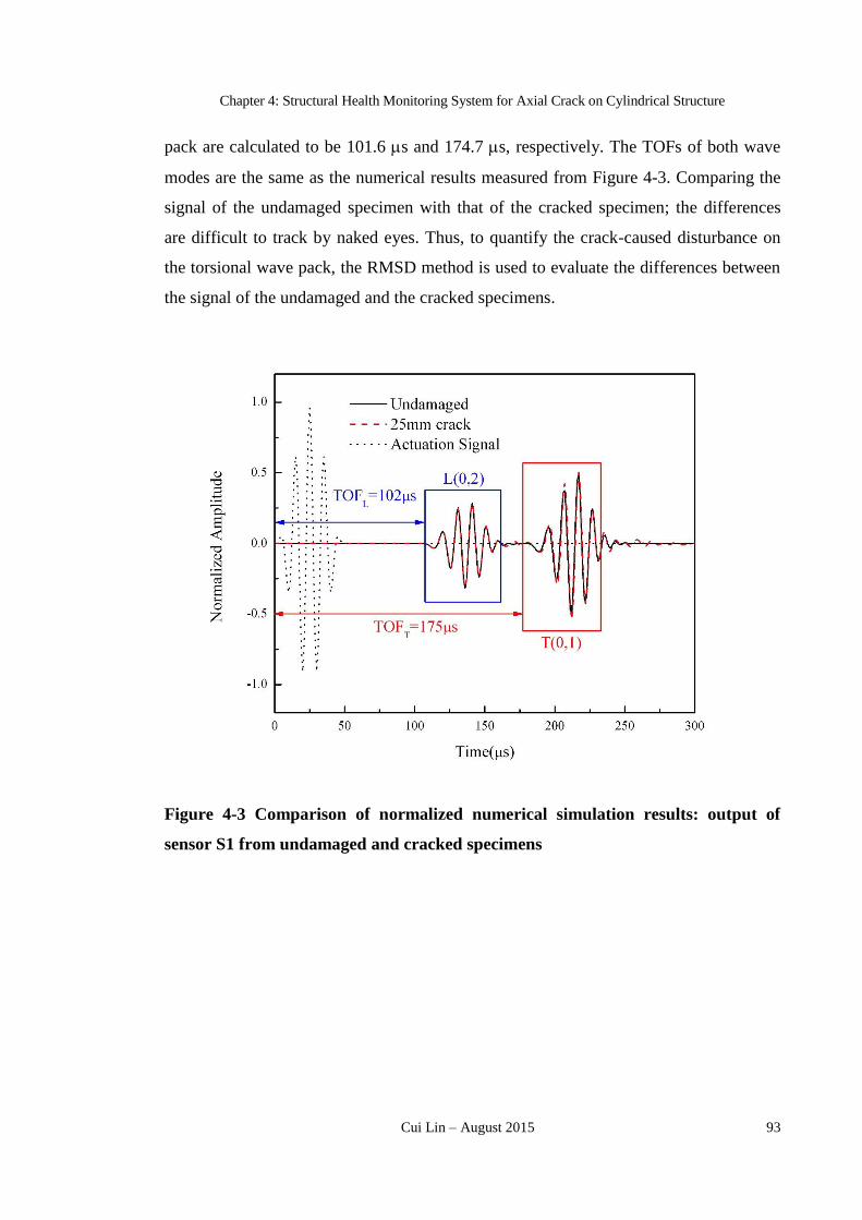
Chapter 4: Structural Health Monitoring System for Axial Crack on Cylindrical Structure
Cui Lin – August 2015 93
pack are calculated to be 101.6 s and 174.7 s, respectively. The TOFs of both wave
modes are the same as the numerical results measured from Figure 4-3. Comparing the
signal of the undamaged specimen with that of the cracked specimen; the differences
are difficult to track by naked eyes. Thus, to quantify the crack-caused disturbance on
the torsional wave pack, the RMSD method is used to evaluate the differences between
the signal of the undamaged and the cracked specimens.
Figure 4-3 Comparison of normalized numerical simulation results: output of
sensor S1 from undamaged and cracked specimens

HEALTH MONITORING OF CYLINDRICAL STRUCTURES USING MFC TRANSDUCERS
94 Cui Lin – August 2015
Figure 4-4 RMSD crack indices from the output of sensor S1 to monitor the axial
direction crack growth (numerical simulation).

Chapter 4: Structural Health Monitoring System for Axial Crack on Cylindrical Structure
Cui Lin – August 2015 95
Take all the numerical simulation output into Eq. 3-3, the RMSD crack index of
torsional wave pack and longitudinal wave pack are compared in Figure 4-4. Just as
expected, torsional wave pack is more sensitive to the crack growth than the
longitudinal wave pack. The linear fit of these RMSD values suggests that the RMSD
value varies linearly with the axial crack length. Hence, it can be conveniently used to
monitor the growth of the axial crack.
4.3.2 Numerical Simulation of Axial Crack Position Identification
The output from sensor S2 is used to identify the position of the axial crack. Results of
the undamaged specimen and the specimen with 25mm axial direction crack are
compared in Figure 4-5. Besides the wave pack directly from the actuator to sensor S2,
two additional wave packs are found, which are the longitudinal wave mode L(0,2) and
the torsional wave mode T(0,1). Just as expected, the torsional wave pack is more
sensitive to the axial crack, and the reflected wave pack is hence larger. As the TOF of
the torsional wave pack can be measured from the graph, and the group speed of the
torsional wave is obtained from the group speed dispersion curve in Figure 3-2, the
position of the crack is thus located. If the distance from actuator to crack position is
denoted by X, it can be calculated by
𝑋 = (𝑇𝑂𝐹∆𝑇 × 𝑉𝑇 − 𝑆𝐴 𝑡𝑜 𝑆2)/2 Eq.4-1
where 𝑇𝑂𝐹∆𝑇 is the TOF of the additional torsional wave pack reflected from the defect;
VT is the group speed of the first order torsional wave mode; and SA to S2 is the A-to-S2
distance . Substitute the additional torsional wave pack TOF of 225s into Eq.4-1, the
estimated crack position is 27.90cm away from the actuator, which is very close to the
exact crack position of 27.5cm from the actuator.
The longitudinal wave pack has also been used to calculate the axial crack position.
However, the reflected longitudinal wave mode from the axial crack is relatively small.
As shown in Figure 4-6, even when the output results have been zoom-in five times
than its original size as plotted in Figure 4-5, it is still tough to identify the centre and
the beginning of the longitudinal wave pack. It leads to an inaccurate reading of
longitudinal wave pack TOF which gives an inaccurate result as compared with the
result calculated from the torsional wave pack. The calculated crack positions from the
longitudinal wave pack and the torsional wave pack are compared with the actual crack

HEALTH MONITORING OF CYLINDRICAL STRUCTURES USING MFC TRANSDUCERS
96 Cui Lin – August 2015
position in Table 4-1 and Table 4-2, respectively. As listed in Table 4-2, using reflected
longitudinal wave pack to calculate the TOF of additional wave pack reflected from
axial direction crack end up with a much greater error.
Table 4-1 Exact axial crack position (calculated based on group speed from
dispersion curve)
Wave
Pack
TOFp
(s) Vp (m/s) SA to S (m)
Calculated crack
position X (m)
Actual crack
position (m)
Error
(%)
L(0,2) 129.3 5412 0.15 0.275 0.275 0
T(0,1) 222.9 3149 0.15 0.275 0.275 0
Table 4-2 Numerical simulation axial crack position
Wave
Pack
TOFp
(s) Vp (m/s) SA to S (m)
Calculated crack
position X (m)
Actual crack
position (m)
Error
(%)
L(0,2) 150 5412 0.15 0.331 0.275 20.3
T(0,1) 225 3149 0.15 0.279 0.275 1.55

Chapter 4: Structural Health Monitoring System for Axial Crack on Cylindrical Structure
Cui Lin – August 2015 97
Figure 4-5 Axial crack position identification from the output of sensor S2
(numerical simulation)
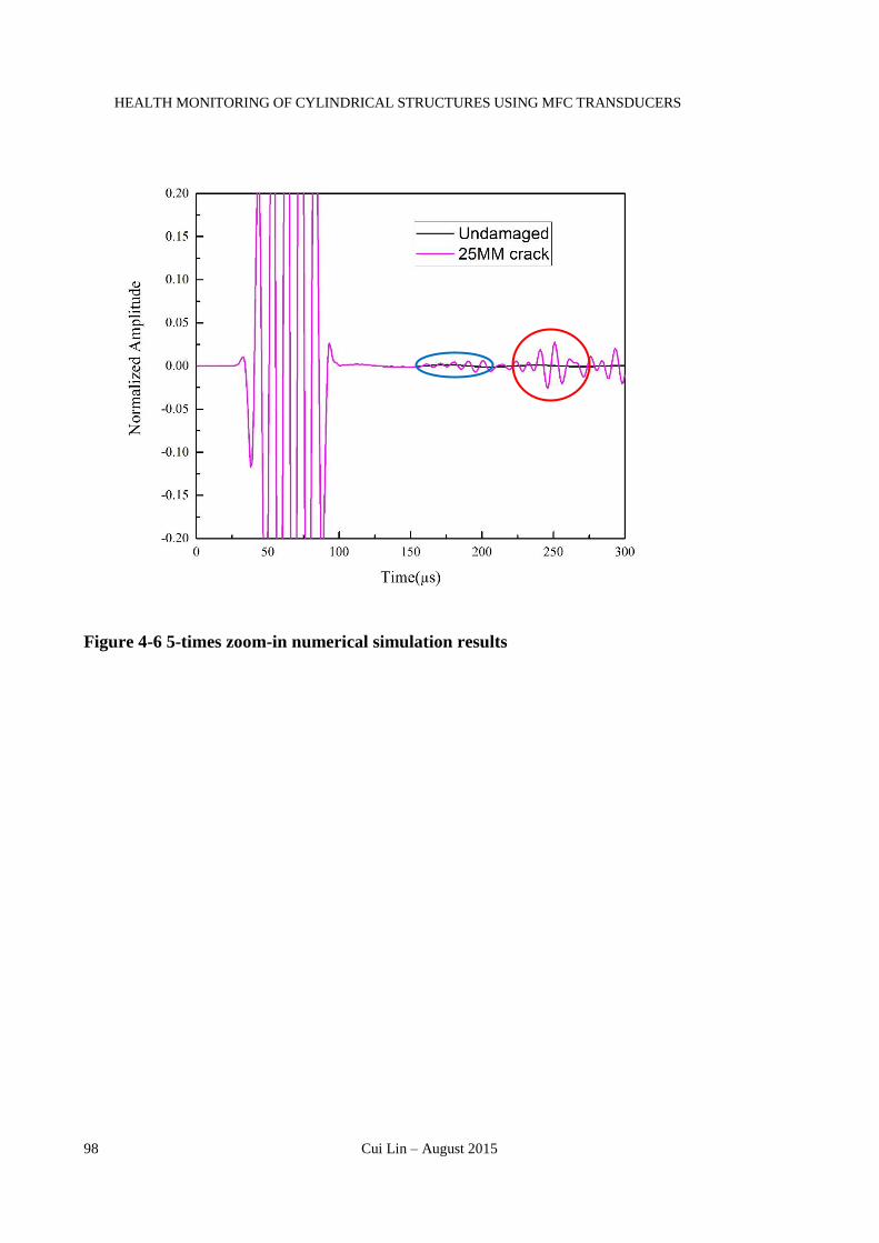
HEALTH MONITORING OF CYLINDRICAL STRUCTURES USING MFC TRANSDUCERS
98 Cui Lin – August 2015
Figure 4-6 5-times zoom-in numerical simulation results

Chapter 4: Structural Health Monitoring System for Axial Crack on Cylindrical Structure
Cui Lin – August 2015 99
4.4 Experimental Study of SHM of Axial Crack Using Torsional
Wave
In the numerical simulation, the specimen is considered to be fully covered by the ring-
shaped actuator by which only the axisymmetric wave modes can be activated. Since in
the experimental study, the MFC patches can only cover part of the circumference, the
flexural wave modes are the concomitance of the axisymmetric wave modes.
4.4.1 Experiment Setup
An aluminum pipe with 2.4m in length, 102mm in outer diameter and 3mm in wall
thickness is used in the experimental study. The aluminum pipe is supported by four
stands at the bottom. Three MFC transducers are bonded to the surface of the tube, 45˚
oriented to the axial direction, as shown in Figure 4-7.

HEALTH MONITORING OF CYLINDRICAL STRUCTURES USING MFC TRANSDUCERS
100 Cui Lin – August 2015
Figure 4-7 Experimental setups for torsional wave SHM of pipe using MFC
transducers
The experimental setup consists of a Tabor Electric ww1701 arbitrary function
generator, a Terk PZD350A high power amplifier, a YOKOGAWA DL1740
Oscilloscope and a National Instruments (NI) integrated digital signal acquisition (DAQ)
system. The MFC actuator is driven by amplified 100V peak-to-peak actuation signals.
The sensors are connected to the NI multi-channel switching box to receive the signal
simultaneously. An additional cable from the function generator is connected to the
DAQ device to synchronize the data acquisition process.
A penetrated crack is initiated at the centre of the pipe with an initial length of 3mm and
a constant width of 3mm. The crack length is increased at 2mm increment until it
reached 49mm which is almost the radius of the pipe. At each crack size, experimental
data within target frequency bandwidth (60 kHz – 200 kHz) are collected. To eliminate
the influence of background noise, 16-times cycle averaging method is used. At low
actuation frequency, the actuation signal will take a longer time to be generated. Hence,
low actuation frequency is equal to ‘wider’ wave pack. To prevent wave packs
overlapping with each other, longer A-to-S distance is needed. At high actuation
frequency, the actuating and sensing capability of MFC is greatly reduced which lowers

Chapter 4: Structural Health Monitoring System for Axial Crack on Cylindrical Structure
Cui Lin – August 2015 101
the accuracy of the SHM results. The lower and upper limit of the frequency bandwidth
is thus set at 60 kHz – 200 kHz according to the dimension of the specimen and the
actuating capability of MFC, respectively. As the DAQ device does not have any power
isolation function, the AC background noise needs to be removed from the original data.
Following the method discussed in section 3.4.2 and Eq.3-4, most the AC background
noise can be eliminated from the data collected by sensors.
4.4.2 Experiment on Axial Crack Size Growth Monitoring
Experimental results of sensor S1 from the undamaged specimen and the specimen with
50mm crack are compared in Figure 4-8.

HEALTH MONITORING OF CYLINDRICAL STRUCTURES USING MFC TRANSDUCERS
102 Cui Lin – August 2015
Figure 4-8 Comparison of experimental results: output of sensor S1 from
undamaged and cracked specimens.

Chapter 4: Structural Health Monitoring System for Axial Crack on Cylindrical Structure
Cui Lin – August 2015 103
Apparently, they are different from the numerical simulation results under the same
actuation frequency of 100 kHz (as shown in Figure 4-3) because the experimental data
are complex due to the existence of flexural waves, which are too complicated to be
separated. However, as the A-to-S1 distance and the group speed of each wave mode
are known, the TOF of each wave mode under 100 kHz actuation frequency can be
calculated. The torsional wave pack T(0,1) and longitudinal wave pack L(0,2) are then
identified and marked in Figure 4-8. Just as expected, the longitudinal wave pack is not
sensitive to the axial crack growth. Compared with the torsional wave pack, the crack
caused change on the longitudinal wave pack is relatively small. The experimental
RMSD crack indices from the torsional wave and the longitudinal wave are calculated
based on Eq.3-3 and plotted in Figure 4-9.

HEALTH MONITORING OF CYLINDRICAL STRUCTURES USING MFC TRANSDUCERS
104 Cui Lin – August 2015
Figure 4-9 RMSD crack indices from output of sensor S1 to monitor the axial
direction crack growth (experimental results)

Chapter 4: Structural Health Monitoring System for Axial Crack on Cylindrical Structure
Cui Lin – August 2015 105
Compared with the RMSD crack indices from numerical simulation, the RMSD crack
indices from the experimental data are more disordered. However, they still suggest a
linear pattern between output signatures changes and crack growth. Compared with the
experimental results listed in Chapter 3, the experimental data in Chapter 4 is using
undamaged specimen as reference baseline signature. Figure 5-9 illustrates again that
the torsional wave pack is more sensitive to axial crack growth than the longitudinal
wave pack.
To reduce scattering of the experimental results, the possible improvements can be:
1) Proper selection of baseline signature
All the experimental data are compared to the baseline signature to compute the
RMSD crack indices. A good baseline signature from the undamaged specimen
is critical to ensure accuracy, Since the DAQ are automatically performed, it is
suggested to have multiple and stable baseline signatures that could be used for
the calculation of RMSD method.
2) Stable experiment environment, setup and boundary conditions.
The data should be collected under similar circumstances. Especially when the
baseline signature is collected, the following data should be collected under the
same environment and boundary condition to limit any uncertainties which may
cause the change of signals. In the experiment, because the crack is created and
expanded on a milling machine, the transducers are disconnected and
reconnected every time the crack is enlarged, which increased the uncertainty of
the change of the signal.
3) Pre-process of signals to remove the background noise
RMSD method highly depends on the quality of signals. The changes of wave
pack can come from defects, change of boundary conditions as well as
background noises. When background noise is not removed from the signals, it
will lead to a higher RMSD value.
4) Dimension of the crack
In the experiment, an axial crack with 3mm width is adopted whereas in the
numerical simulation an ideal axial crack with zero width is considered. The
circumferential dimension of the crack also contributed to the change of RMSD
value.

HEALTH MONITORING OF CYLINDRICAL STRUCTURES USING MFC TRANSDUCERS
106 Cui Lin – August 2015
5) Dimension of MFC
In the numerical study, a ring-shaped actuator is simulated. The actuation only
worked at a single axial position of the pipe. The sensor output is also from a
single point. In the experiment, MFC transducer covered certain area to actuate,
and the sensor output is also the average result of the covered area, which
increased the difficulty of interpreting the signatures.
Compared with the RMSD crack indices from the torsional wave pack, the RMSD crack
indices from the longitudinal wave pack showed a more scattered pattern. This
phenomenon is because the disturbance of axial crack on the longitudinal wave pack is
very tiny, so the RMSD value is easily affected by any noise or change in boundary
condition
4.4.3 Experiment of Axial Crack Position Identification
The numerical simulation used a simplified ring-shaped actuator which can only
generate axisymmetric wave modes. However, in the experiment under partial actuation
condition, the flexural wave modes are also included in the output signatures. The
experimental results of sensor S2 from the undamaged specimen, the specimen with
3mm crack, and the specimen with 8mm crack have been compared in Figure 4-10.

Chapter 4: Structural Health Monitoring System for Axial Crack on Cylindrical Structure
Cui Lin – August 2015 107
Figure 4-10 Comparison of experimental results: output of sensor S2 from
undamaged and cracked specimens

HEALTH MONITORING OF CYLINDRICAL STRUCTURES USING MFC TRANSDUCERS
108 Cui Lin – August 2015
Unlike the numerical simulation results are shown in Figure 4-5, the experimental
output signature of sensor S2 is rather complicated. As shown in Figure 4-10, the
additional signal reflected from the axial crack is buried inside the flexural wave modes
following behind (color shade zone). To use Eq.4-1 to calculate the crack position, the
additional reflected torsional wave pack needs to be identified before the TOF of the
wave pack can be obtained.
4.4.3.1 Mode Separation
Since there is no crack existing in between the actuator and sensor S2, the direct-passed
wave packs measured by S2 from the cracked and undamaged specimen are the same
regarding amplitude and phase if the actuations are the same. Using the signature from
the undamaged specimen as a reference, the signals from the cracked specimen are
subtracted from the baseline signature and the residual signals are then assumed to be
the crack affected signals. Figure 4-11 compares three residual signals: (1) the
‘undamaged’ signal is the residual of two different baseline signatures of the
undamaged specimen; (2) the ‘3mm crack’ signal is the residual of subtracting a signal
of undamaged specimen from the signal of the specimen with 3mm crack; and (3) the
‘8mm crack’ signal is similarly obtained as the ‘3mm crack’ signal. The ‘undamaged’
residual is considered as noise whose amplitude is covered by the shadowed area. Any
residual wave pack, whose peak amplitude is less than the ‘undamaged’ level or the
noise level, is considered nil and the structures are considered healthy. Once the crack is
initiated, as shown in Figure 4-11, additional reflected wave pack from the axial crack,
which exceeds the noise level, can be detected. As compared with the ‘3mm crack’
residual, the ‘8mm crack’ residual includes a larger torsional wave pack regarding both
amplitude and wave pack width, while the included longitudinal wave pack remains
almost the same as that in the ‘3mm crack’ residual. This phenomenon is because when
the axial crack size is growing, its axial dimension increases but its circumferential
dimension remains constant. Thus, the longitudinal wave pack is less affected than the
torsional wave pack.
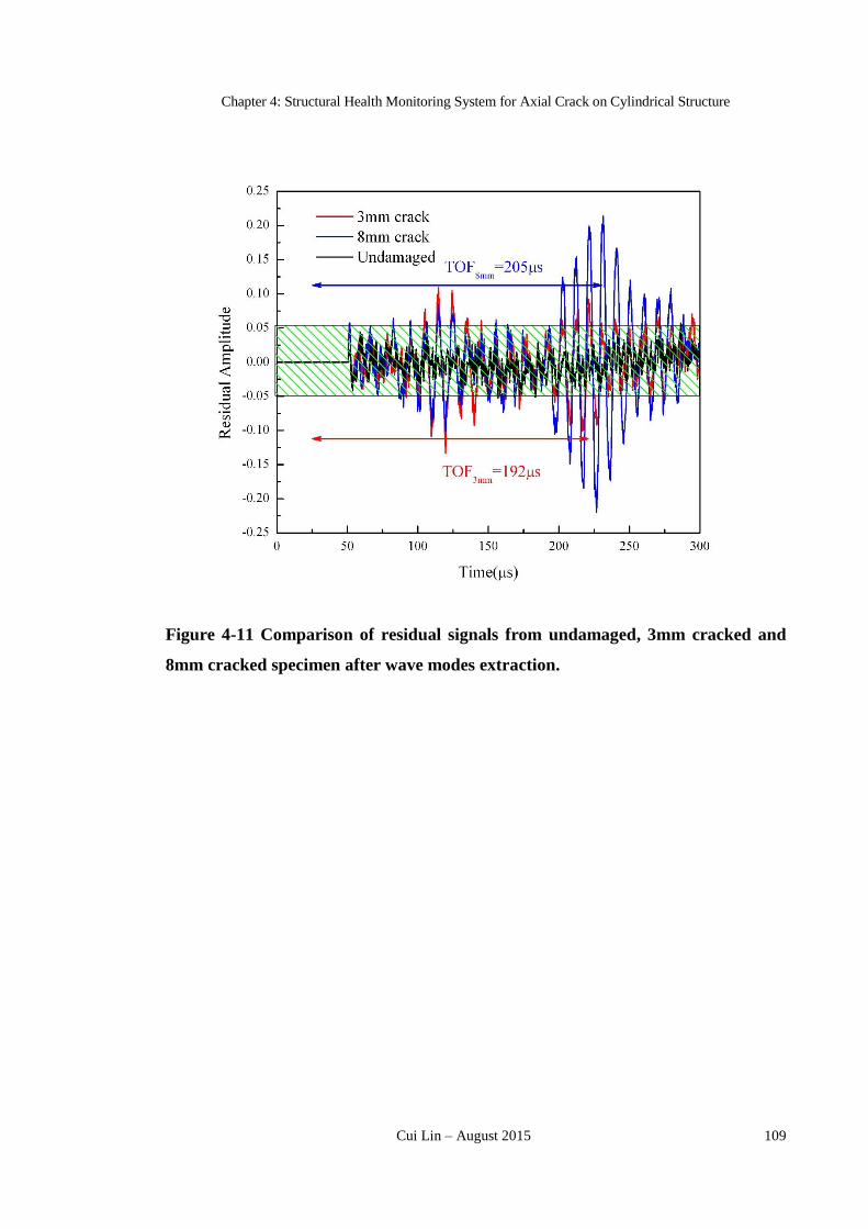
Chapter 4: Structural Health Monitoring System for Axial Crack on Cylindrical Structure
Cui Lin – August 2015 109
Figure 4-11 Comparison of residual signals from undamaged, 3mm cracked and
8mm cracked specimen after wave modes extraction.
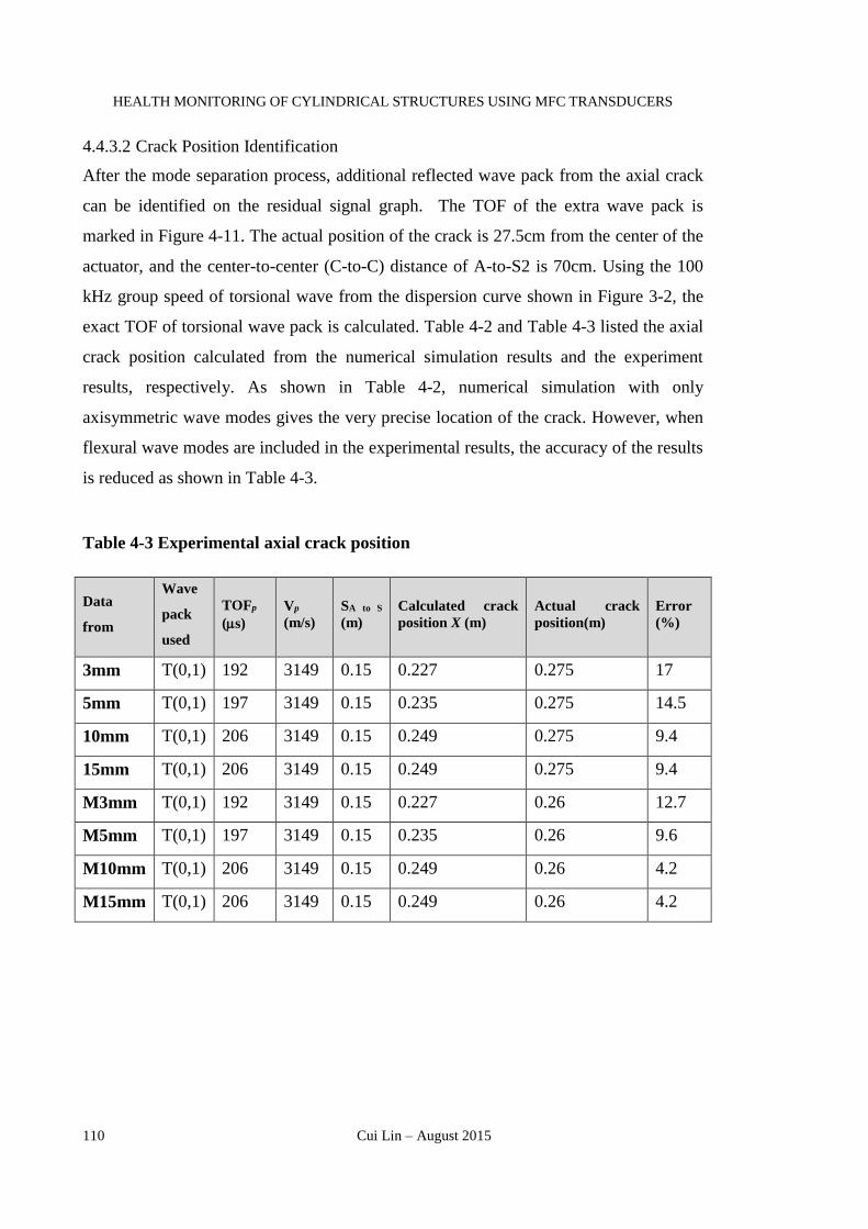
HEALTH MONITORING OF CYLINDRICAL STRUCTURES USING MFC TRANSDUCERS
110 Cui Lin – August 2015
4.4.3.2 Crack Position Identification
After the mode separation process, additional reflected wave pack from the axial crack
can be identified on the residual signal graph. The TOF of the extra wave pack is
marked in Figure 4-11. The actual position of the crack is 27.5cm from the center of the
actuator, and the center-to-center (C-to-C) distance of A-to-S2 is 70cm. Using the 100
kHz group speed of torsional wave from the dispersion curve shown in Figure 3-2, the
exact TOF of torsional wave pack is calculated. Table 4-2 and Table 4-3 listed the axial
crack position calculated from the numerical simulation results and the experiment
results, respectively. As shown in Table 4-2, numerical simulation with only
axisymmetric wave modes gives the very precise location of the crack. However, when
flexural wave modes are included in the experimental results, the accuracy of the results
is reduced as shown in Table 4-3.
Table 4-3 Experimental axial crack position
Data
from
Wave
pack
used
TOFp
(s)
Vp
(m/s)
SA to S
(m)
Calculated crack
position X (m)
Actual crack
position(m)
Error
(%)
3mm T(0,1) 192 3149 0.15 0.227 0.275 17
5mm T(0,1) 197 3149 0.15 0.235 0.275 14.5
10mm T(0,1) 206 3149 0.15 0.249 0.275 9.4
15mm T(0,1) 206 3149 0.15 0.249 0.275 9.4
M3mm T(0,1) 192 3149 0.15 0.227 0.26 12.7
M5mm T(0,1) 197 3149 0.15 0.235 0.26 9.6
M10mm T(0,1) 206 3149 0.15 0.249 0.26 4.2
M15mm T(0,1) 206 3149 0.15 0.249 0.26 4.2

Chapter 4: Structural Health Monitoring System for Axial Crack on Cylindrical Structure
Cui Lin – August 2015 111
Figure 4-12 Modified wave propagation path length
The low accuracy of the position identification is also due to the distance of actuator to
crack used in Eq.4-1. In the numerical simulation, the transducers ha4ve exact axial
positions, but in the experiment, the transducers cover parts of the pipe in the axial
direction, which increases the complexity of the output signals. As shown in Figure
4-12, taking the transducer’s dimension into consideration, the actuator to crack
distance is changed from 27.5cm to 26cm. The corrected results, using the new value in
Eq.4-1, are also listed in Table 4-3. Apparently, their accuracy improved greatly. It is
also found from Table 4-3 that, as the crack size increases, the accuracy of the crack
position identification also increases. This phenomenon is because when the crack size
is small, the wave pack reflected from the crack is also small in amplitude and it is hard
to determine the center of the wave pack, which reduced the accuracy. As the crack size
increases, the reflected wave pack amplitude also increases due to the larger disturbance
and the wave pack is thus easier to measure.
4.4.4 Sensitivity range of the MFC transducers
Each type of transducers has its own sensing range. If the transducers are located out of
its recommended sensing range either the results is unreliable or there is no results at all.
HEALTH MONITORING OF CYLINDRICAL STRUCTURES USING MFC TRANSDUCERS
112 Cui Lin – August 2015
In this study, no MFC transducer sensitivity study is covered. The actuator to sensor
distance is fixed because of following reasons:
1. Input energy.
The input energy is critical to MFC type of transducers. There is a suggested working
voltage for MFC transducers from the manufacture. For P1 type MFC the maximum
working voltage is from -500V to +1500V. The higher driving voltage is used, the
larger response we can expect. However, at the same time, at a higher driving voltage,
the signal is easy to be distorted after amplification. To be noted the original actuation
signal is generated from the digital function generator and enlarged by the signal
amplifier. The amplified driving signal will be then applied to the MFC actuators. Most
of the time, there is a limitation on the signal amplifier where the actuation frequency
and output voltage both have an upper bound. The amplifier used in the experiment
setup TREK 350A. The specs mentioned that the amplifier is good for ±350V AC and
up to 250kHz signal. Even though we wanted to carry out experiment study on the
sensitivity of the input signal, we were limited by the equipment setup. Our amplifier
cannot drive the MFC to its full capacity hence we can only amplify the signal to the
current voltage level where the driven signal still maintains the wave shape we want. If
higher actuation voltage or frequency is used, the amplified actuation signal can no
longer maintain the designed wave shape; more disturbance will be included in the
output signals. We also carry out an experiment with actuation frequency at 300kHz.
The results showed that the amplifier greatly distorts the signal, and no recognized
pattern can be used for the crack growth monitoring process.
2. Testing Specimen.
In this study, there are two types of testing specimens used: the 1.2m length specimen
and the 2.4m length specimen. The 1.2m length specimen is initially used to perform the
longitudinal crack growth monitoring task that described in Chapter 3. Then, 2.4m
specimens are used to detect both the location and crack growth that described in
Chapter 4. The reason not to use 1.2m specimen in Chapter 4 experiment study is to
eliminate the wave reflection from specimen open end which is not occurred in
continuous pipeline structures. Because of the space limitation of laboratory and the
milling machine that initiate the crack on the specimen, 2.4m length specimen is the
maximum length that can be tested in current experiment setup. In this study, torsional

Chapter 4: Structural Health Monitoring System for Axial Crack on Cylindrical Structure
Cui Lin – August 2015 113
wave pack is the priority target wave pack since it is not dispersive during propagation.
Hence it is good to be used for range sensitivity test. However, due to the low travel
speed of the torsional wave, it is easy to be interference by other faster wave modes that
reflected from free boundaries. Hence, it is not practical to carry out experiment study
on the sensitivity range of MFC transducers.
3. Wave attenuation
There is wave attenuation during propagation. The wave attenuation is because of the
energy is absorbed or dispersed during propagation. There are so many uncertainties
that will cause the attenuation. The attenuation may be because of the host material
properties, the pressure, the temperature, the content the host structure is carrying, the
boundary conditions, etc.
4.5 Summary and Conclusion
This chapter presents a close-loop self-sensing and monitoring system for an axial crack
in cylindrical structures. Different from Chapter 3, this chapter developed the SHM
system that is capable of detecting both axial oriented crack’s dimension and position.
Since the particle motion direction of torsional wave modes is perpendicular to the
orientation of axial cracks, torsional wave pack is more sensitive to axial crack. In this
system, MFC is placed 45 degrees clockwise oriented against the axis of the cylinder to
generate torsional wave packs. The MFC transducer at the center works as the actuator;
the other two MFC transducers operate as sensors to detect the axial position of the
crack and to monitor the crack size growth, respectively. Five-cycle Hanning windowed
sine wave tone burst was used to activate guided waves in the cylindrical structures.
With the help of its concentrated wave pack center, the accuracy of locating the crack
position is improved; and with its narrowed bandwidth, the dispersion effect of wave
modes is limited. To monitor the crack growth, RMSD method is adopted to correlate
the crack growth to the total waveform changes, where a linear pattern between the
RMSD index and the crack size is observed. TOF based method is adopted to find the
axial position of the crack in the cylindrical structures. To eliminate the effect of
flexural waves, the residual signal whereby the signal of the undamaged specimen is
subtracted from the signal of cracked specimen is used.

HEALTH MONITORING OF CYLINDRICAL STRUCTURES USING MFC TRANSDUCERS
114 Cui Lin – August 2015
Both numerical simulation and experimental investigation are conducted. The results
show that both the axial position and crack size growth of the axial crack can be well
located/monitored using this close-loop sensing system. In the experimental
investigation, the existence of flexural waves, changes of boundary conditions, errors in
data processing procedure, etc., all contributed to the reduced accuracy of the results as
compared with the numerical simulation. Nevertheless, the experimental data still show
promise in the SHM of axial crack in cylindrical structures.
For the monitoring of continuous cylindrical structures, an integrated intelligent SHM
system can be further developed based on the proposed close-loop self-sensing system.
To further develop the SHM system to achieve continuous cylindrical structures
monitoring, optimized placement of transducers and artificial intelligence to integrate
automatic data acquisition with data processing and result analysis are needed.
Furthermore expansion of this ‘smart’ system is discussed in Chapter 5.

Chapter 5: The Identification of Crack Orientation and Dimension on Cylindrical Structure
Cui Lin – August 2015 115
5 THE IDENTIFICATION OF
CRACK ORIENTATION AND
DIMENSION ON
CYLINDRICAL STRUCTURE
5.1 Introduction
In cylindrical structures, there are many types of guided waves. The most commonly
discussed are the two fundamental axisymmetric waves: torsional waves and
longitudinal waves. There are also many complicated non-axisymmetric wave modes
existing, like flexural wave modes. Usually at certain actuation frequency range (below
200 kHz), only limited wave modes can be dominated in the overall wave shape and
show their characters during propagation. Because the particle movement direction of
torsional wave modes are perpendicular to the axis, and the particle movement direction
of longitudinal wave modes are parallel to the axis of the cylindrical structure, when the
crack on the structure is axial oriented, the torsional wave packs are more easily
affected by the crack than the longitudinal wave packs. Due to MFC’s ease to bend and
ease to be driven characters, MFC is used as transducers to activate and receive signals.
In Chapter 3, a new axial oriented crack growth monitoring system is proposed based on
MFC generated torsional waves. The close-loop system can pick up the axially oriented
crack growth on a cylindrical structure. RMSD crack index is proposed to be used to
quantify the signal change and correlated the change with the crack size change.

HEALTH MONITORING OF CYLINDRICAL STRUCTURES USING MFC TRANSDUCERS
116 Cui Lin – August 2015
Chapter 4 proposed an expanded system based on the system developed in Chapter 3.
With one additional sensor placed next to the actuator, the new regime can pick up both
the axially oriented crack growth and its location. The increase of crack will be
monitored based on RMSD crack index, and the location of the crack will be estimated
based on the pulse-echo method.
All the works described in Chapter 3 and Chapter 4 are focused on axially oriented
crack only. The reason is that the torsional wave is sensitive to the change of axially
oriented crack. The high sensitivity of torsional wave on axially oriented crack comes
from the particle motion direction is perpendicular to the crack orientation. On the other
hand, the longitudinal wave is also sensitive to circumferential direction crack. These
two types of crack are most commonly occurred cracks on the cylindrical structure. This
chapter is focusing on developing a system that can be used for crack size and
orientation identification of line type crack on cylindrical structures.
5.2 Method of Study
The governing equation of wave propagation in hollow cylinders is first given by Gazis
(Gazis 1959a, Gazis 1959b). The wave propagating in cylindrical structures can be
grouped into axisymmetric wave modes and non-axisymmetric wave modes based on
their particle motion (PM) directions. As shown in Figure 5-1, there are two types of
axisymmetric wave modes, namely longitudinal wave modes and torsional wave modes.
The PM of a longitudinal wave is parallel to the axis of the hollow cylinder, and only
the axial displacement (uz) is included. On the other hand, the PM of the torsional wave
is perpendicular to the axis, where only the circumferential displacement (u) is
included.
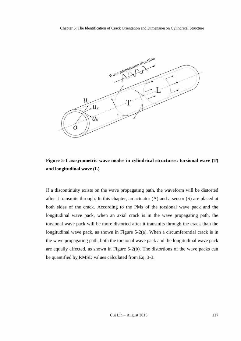
Chapter 5: The Identification of Crack Orientation and Dimension on Cylindrical Structure
Cui Lin – August 2015 117
Figure 5-1 axisymmetric wave modes in cylindrical structures: torsional wave (T)
and longitudinal wave (L)
If a discontinuity exists on the wave propagating path, the waveform will be distorted
after it transmits through. In this chapter, an actuator (A) and a sensor (S) are placed at
both sides of the crack. According to the PMs of the torsional wave pack and the
longitudinal wave pack, when an axial crack is in the wave propagating path, the
torsional wave pack will be more distorted after it transmits through the crack than the
longitudinal wave pack, as shown in Figure 5-2(a). When a circumferential crack is in
the wave propagating path, both the torsional wave pack and the longitudinal wave pack
are equally affected, as shown in Figure 5-2(b). The distortions of the wave packs can
be quantified by RMSD values calculated from Eq. 3-3.
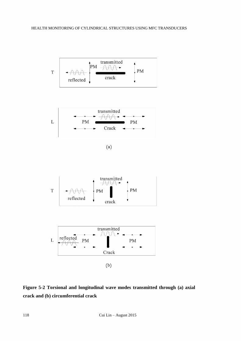
HEALTH MONITORING OF CYLINDRICAL STRUCTURES USING MFC TRANSDUCERS
118 Cui Lin – August 2015
Figure 5-2 Torsional and longitudinal wave modes transmitted through (a) axial
crack and (b) circumferential crack

Chapter 5: The Identification of Crack Orientation and Dimension on Cylindrical Structure
Cui Lin – August 2015 119
In this chapter, these different behaviors and RMSD values for the various wave packs
(torsional and longitudinal) transmitted through the different cracks (axial and
circumferential) are used to determine the crack size and orientation.
To be noticed that Chapter 3 is the initial experiment proposal with the original
experiment setup: the transducers are placed on both side of the crack, one as an
actuator and the other as a sensor. The purpose is to monitor the crack growth use the
first torsional wave pack that generated by the actuator. The sensor will catch the signal
that affected by the crack and the proposed method will identify the changes in the
targeting wave pack and correlated the crack changes with the signal changes. As per
the conclusion of Chapter 3, this experiment setup successfully monitored the
development of longitudinal direction crack.
In Chapter 3, the axially oriented crack growth is successfully monitored. Based on the
results in Chapter 3, Chapter 4 is aimed to identify the crack location on the specimen at
the same time of monitoring the crack growth. Longer specimen is used in the
experiment. Pulse-echo method is used to detect the crack location. The longer
specimen will increase the wave propagation path and it will not only be beneficial to
the separation of different wave packs but also more close to the actual condition of
“continuous” pipeline. To be noted that in lab testing environment, it is extremely hard
to carry out an experiment on continuous pipelines health monitoring. Hence, the longer
specimen will be helpful on separating (eliminating) the wave pack reflected from the
open end. Compared with testing specimen used in Chapter 3, the crack is still placed at
the center of the specimen. The actuator to sensor distance is almost the same. The only
difference between the specimens used in these two chapters is the length of the
specimen before the actuator (left) and after the sensor (right). Since longitudinal wave
pack travels faster than the torsional wave pack, the aim of such setup is to ensure the
torsional wave pack for crack growth monitoring and crack position identification is not
overlapped with the longitudinal wave pack reflected from the open end. Based on the
experiment setup, the wave propagation path has been increased which will contribute
to the separation of targeting wave packs. In actual continuous pipelines, there is no
such open “termination” under operation condition. Hence there is no reflection from
discontinuity other than reflections from the crack. Using a longer specimen make the
experiment more close to the actual condition (without reflection from open end).

HEALTH MONITORING OF CYLINDRICAL STRUCTURES USING MFC TRANSDUCERS
120 Cui Lin – August 2015
Since the longitudinal oriented crack growth and crack location identification have been
proved to be able to monitor by proposed method, chapter 5 is focusing on detection of
crack with any orientation and dimension. More specimens with different crack
orientations were tested. The lathering machine is used to initiate crack on the specimen
and then enlarge it. Whenever crack is required to be enlarged, cables had to be
disconnected from the testing specimen and the specimen needs to be taken to the
machine for machinery. Since more specimens are required to be tested, if the long
specimen is used, it would greatly increase the duration and the effort on the machinery
part. Based on the experiment design concept, the first torsional wave pack, and the first
longitudinal wave pack is what we required. Even though there might be some other
wave packs reflected from the open end due to shortened wave propagation path from
shortened specimen, it is still effective when using the targeted wave packs for crack
orientation and size monitoring.
5.3 RMSD Crack Index
The effects of various cracks on the different wave packs, which are described in the
last section, are quantitatively analyzed through both numerical simulation and
experimental test. A T6061 aluminium pipe with a length of 1200 mm, the inner radius
of 48 mm, and the wall thickness of 3 mm is used for this test. The MFC patches are
attached at 45-degree orientation about the centroid axis of the pipe. As shown in Figure
5-3, the transducers are placed 300 mm from the free end of the specimen. The actuator
to sensor (A-to-S) distance is 600 mm and the actuator to crack (A-to-C) distance is 200
mm. In the application, only the first few wave packs are considered, i.e., the wave
packs directly from the actuator to the sensor. Such transducers distribution avoids wave
packs reflected from free end (arrive later) overlapped with the target wave packs
(arrive earlier).
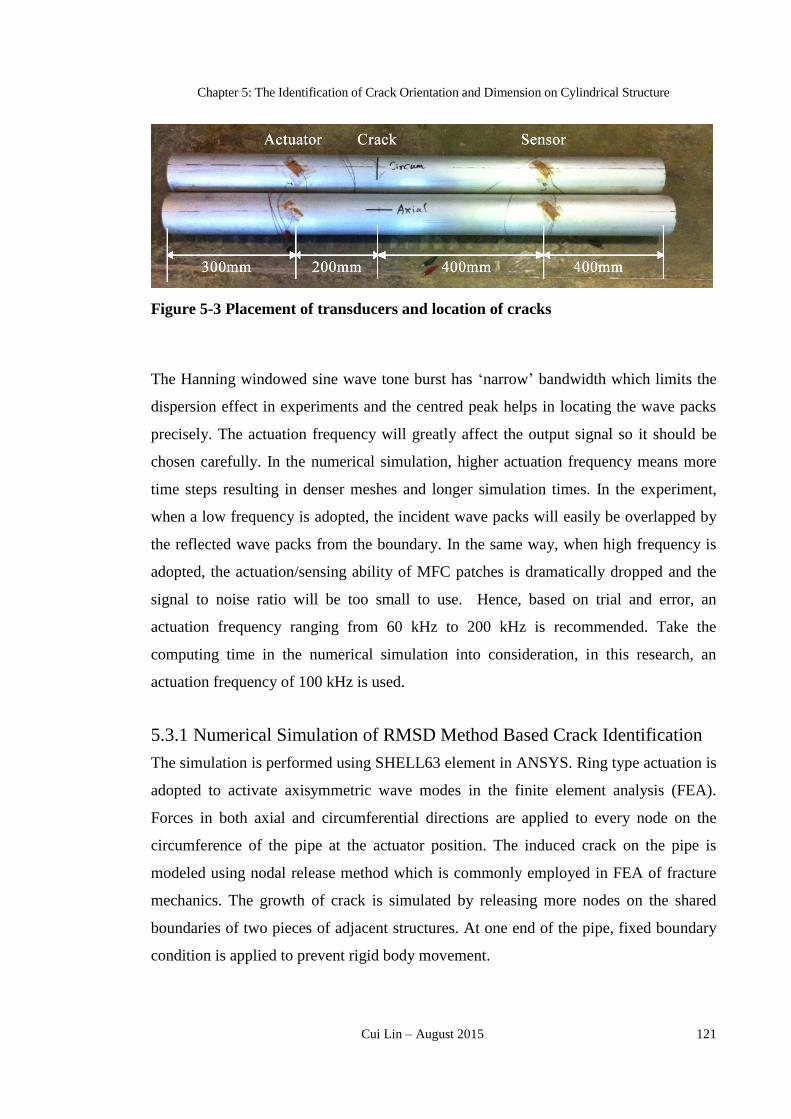
Chapter 5: The Identification of Crack Orientation and Dimension on Cylindrical Structure
Cui Lin – August 2015 121
Figure 5-3 Placement of transducers and location of cracks
The Hanning windowed sine wave tone burst has ‘narrow’ bandwidth which limits the
dispersion effect in experiments and the centred peak helps in locating the wave packs
precisely. The actuation frequency will greatly affect the output signal so it should be
chosen carefully. In the numerical simulation, higher actuation frequency means more
time steps resulting in denser meshes and longer simulation times. In the experiment,
when a low frequency is adopted, the incident wave packs will easily be overlapped by
the reflected wave packs from the boundary. In the same way, when high frequency is
adopted, the actuation/sensing ability of MFC patches is dramatically dropped and the
signal to noise ratio will be too small to use. Hence, based on trial and error, an
actuation frequency ranging from 60 kHz to 200 kHz is recommended. Take the
computing time in the numerical simulation into consideration, in this research, an
actuation frequency of 100 kHz is used.
5.3.1 Numerical Simulation of RMSD Method Based Crack Identification
The simulation is performed using SHELL63 element in ANSYS. Ring type actuation is
adopted to activate axisymmetric wave modes in the finite element analysis (FEA).
Forces in both axial and circumferential directions are applied to every node on the
circumference of the pipe at the actuator position. The induced crack on the pipe is
modeled using nodal release method which is commonly employed in FEA of fracture
mechanics. The growth of crack is simulated by releasing more nodes on the shared
boundaries of two pieces of adjacent structures. At one end of the pipe, fixed boundary
condition is applied to prevent rigid body movement.

HEALTH MONITORING OF CYLINDRICAL STRUCTURES USING MFC TRANSDUCERS
122 Cui Lin – August 2015
Figure 5-4 compares the normalized output from an undamaged specimen with outputs
from two cracked specimens which are 46 mm circumferential crack and 45mm axial
crack, respectively. In the three cases, the actuator to sensor distance is unchanged; the
wave propagation paths are the same. All wave modes speed can be calculated from the
frequency governing equations (Gazis 1959a, Gazis 1959b) as listed in Table 5-1. The
time of flight of the second ordered longitudinal wave L(0,2) and first order torsional
wave T(0,1) are approximately 110 s and 190 s, respectively. The group speed of
L(0,2) and T(0,1) that transmitted in this aluminum pipe under 100 kHz actuation is
calculated from the frequency governing equations as listed in Table 5-1.
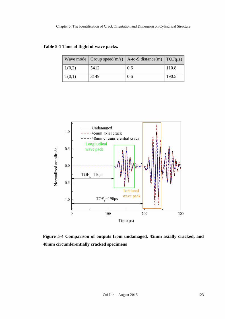
Chapter 5: The Identification of Crack Orientation and Dimension on Cylindrical Structure
Cui Lin – August 2015 123
Table 5-1 Time of flight of wave packs.
Wave mode Group speed(m/s) A-to-S distance(m) TOF(s)
L(0,2) 5412 0.6 110.8
T(0,1) 3149 0.6 190.5
Figure 5-4 Comparison of outputs from undamaged, 45mm axially cracked, and
48mm circumferentially cracked specimens

HEALTH MONITORING OF CYLINDRICAL STRUCTURES USING MFC TRANSDUCERS
124 Cui Lin – August 2015
Figure 5-5 Extracted upper envelope of signals in Figure 5-4

Chapter 5: The Identification of Crack Orientation and Dimension on Cylindrical Structure
Cui Lin – August 2015 125
As compared with the ideal TOF listed in Table 5-1, the TOF of both torsional and
longitudinal wave packs obtained from Figure 5-4 are almost identical. As observed
from Figure 5-4, the wave patterns of the results from the three sets of data are quite
similar. Figure 5-5 extracted the upper envelope of the signals from Figure 5-4. The
extracted envelope clearly showed that axial crack has only a slight effect on the
longitudinal wave pack but has much effect on the torsional wave pack. Substituting the
numerical simulation results into Eq.3-3, the four RMSD crack indices calculated from
longitudinal and torsional wave packs transmitted through the circumferential and axial
cracks are obtained and plotted in Figure 5-6.

HEALTH MONITORING OF CYLINDRICAL STRUCTURES USING MFC TRANSDUCERS
126 Cui Lin – August 2015
Figure 5-6 RMSD crack indices of both circumferential crack and axial crack
(based on numerical simulation)

Chapter 5: The Identification of Crack Orientation and Dimension on Cylindrical Structure
Cui Lin – August 2015 127
According to Figure 5-6, the certain pattern can be recognized between the RMSD
values and the crack sizes. A linear relationship is the simplest and the most convenient
way to correlate the RMSD values to the crack sizes. Linear regression is conducted
using MATLAB, and the slopes are thus obtained. The effectiveness of the linear
regression has been checked by the coefficient of determination (COD) or R2 values.
The closer R2 is to 1, the better the linear regression. Table 5-2 compared the COD
value of the four linear regressions, which clearly shows that the axial crack has only
limited effect on the longitudinal wave but many effects on the torsional wave.
Table 5-2 Parameter of linear regression.
Wave mode Crack orientation Slope COD(R2)
Longitudinal Axial 0.0011 0.995
Torsional Axial 0.0083 0.990
Longitudinal Circumferential 0.0077 0.993
Torsional Circumferential 0.0088 0.996
The slope difference is because the PM of longitudinal wave is not disturbed by the
presence of axial crack but as the PM of torsional wave is perpendicular to the axial
crack, it is greatly affected, as shown in Table 5-1. Comparing to axial crack, the
presence of circumferential crack caused discontinuity on the wave propagating path of
both longitudinal and torsional waves, so it affected both the wave packs.
5.3.2 Experiment Verification of RMSD Method Based Crack
Identification

HEALTH MONITORING OF CYLINDRICAL STRUCTURES USING MFC TRANSDUCERS
128 Cui Lin – August 2015
Figure 5-7 Experimental setup
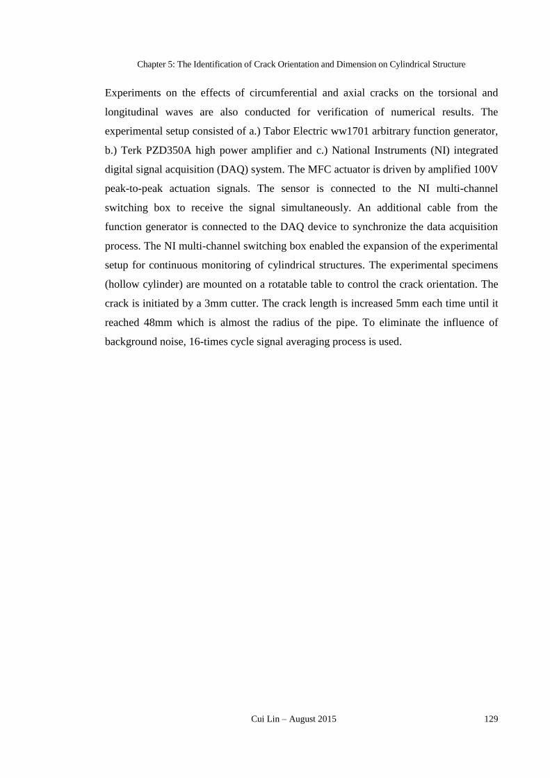
Chapter 5: The Identification of Crack Orientation and Dimension on Cylindrical Structure
Cui Lin – August 2015 129
Experiments on the effects of circumferential and axial cracks on the torsional and
longitudinal waves are also conducted for verification of numerical results. The
experimental setup consisted of a.) Tabor Electric ww1701 arbitrary function generator,
b.) Terk PZD350A high power amplifier and c.) National Instruments (NI) integrated
digital signal acquisition (DAQ) system. The MFC actuator is driven by amplified 100V
peak-to-peak actuation signals. The sensor is connected to the NI multi-channel
switching box to receive the signal simultaneously. An additional cable from the
function generator is connected to the DAQ device to synchronize the data acquisition
process. The NI multi-channel switching box enabled the expansion of the experimental
setup for continuous monitoring of cylindrical structures. The experimental specimens
(hollow cylinder) are mounted on a rotatable table to control the crack orientation. The
crack is initiated by a 3mm cutter. The crack length is increased 5mm each time until it
reached 48mm which is almost the radius of the pipe. To eliminate the influence of
background noise, 16-times cycle signal averaging process is used.

HEALTH MONITORING OF CYLINDRICAL STRUCTURES USING MFC TRANSDUCERS
130 Cui Lin – August 2015
Figure 5-8 Comparison of initial experimental result and modified experimental
result

Chapter 5: The Identification of Crack Orientation and Dimension on Cylindrical Structure
Cui Lin – August 2015 131
As the DAQ device lacks a power isolation module, the AC background noise is also
included in the received signals. However, as the frequency (50 Hz) and the neutral
position (0 V) of the AC noised are known, this AC noise can be removed by curve
fitting. The modified signal is compared with the original signal and the fitted AC noise
in Figure 5-8. Comparing with the numerical simulation result, which has only the
axisymmetric wave modes (L and T), the experimental data included the flexural wave
modes, and thus, the dispersion effect is much greater. Figure 5-8 shows that even
though the non-axisymmetric wave modes greatly messed up the axisymmetric wave
modes, the L(0,2) and T(0,1) wave packs are still recognizable based on the TOF.

HEALTH MONITORING OF CYLINDRICAL STRUCTURES USING MFC TRANSDUCERS
132 Cui Lin – August 2015
Figure 5-9 RMSD crack indices of both circumferential crack and axial
crack(based on experimental result)

Chapter 5: The Identification of Crack Orientation and Dimension on Cylindrical Structure
Cui Lin – August 2015 133
Substituting the experimental results into Eq.3-3, the four RMSD crack indices of
experimental results are calculated and plotted in Figure 5-9. Because of the existence
of flexural wave modes, the slope and sensitivity of the crack indices are slightly
different from the numerical simulation.
The RMSD crack indices obtained from numerical simulation and experimental results
are shown the following features:
1.) Axial crack has little influence on transmitted longitudinal wave packs but has a
significant effect on transmitted torsional wave pack.
2.) Circumferential crack has a significant effect on both transmitted longitudinal and
torsional wave packs.
5.4 Identification of Crack Size and Orientation
Different cracks on the wave propagation path will have different consequences for the
transmitted wave packs. As shown in Figure 5-2, axial crack only causes a discontinuity
in torsional wave-particle motions but has little effect on longitudinal waves.
Circumferential crack causes a discontinuity in both torsional and longitudinal wave-
particle motions. Thus, both wave packs are greatly affected. The RMSD crack indices
connected the crack size growth with the RMSD value change. If crack orientation is
initiated on the pipe in between the circumferential and axial directions, the RMSD
crack indices can also be obtained from the circumferential and axial crack indices.
Both the crack size and orientation can be achieved from the RMSD value of the wave
target packs.
5.4.1 Crack Index for Crack with Any Orientation
Based on RMSD Crack Indices obtained from both axial and circumferential cracks, the
effects when the torsional and longitudinal wave passes through an axial crack (with
length l ) and an additional part related to both length l and orientation This extra part
came from (1) the difference in the effects when a wave pack passes through an axial
crack and a circumferential crack (KTA-KTC or KLA-KLC) and (2) the difference in the
geometry of a slant crack from an axial crack, that is, the slant crack has a
circumferential component l·sinThe RMSD crack index of a slant crack with length l
and orientation can thus be calculated as

HEALTH MONITORING OF CYLINDRICAL STRUCTURES USING MFC TRANSDUCERS
134 Cui Lin – August 2015
{𝑅𝑇
𝑅𝐿} = [
𝐾𝑇𝐴 𝐾𝑇𝐴 − 𝐾𝑇𝐶
𝐾𝐿𝐴 𝐾𝐿𝐴−𝐾𝐿𝐶] {
𝑙𝑙 ∙ 𝑠𝑖𝑛𝜃
} Eq.5-1
where R represents the RMSD value; K is the slope of the RMSD crack index
determined in the previous section. The subscript C and A represent the circumferential
and axial cracks, respectively; the subscript T and L represent the RMSD value
calculated from the torsional and longitudinal wave packs, respectively; and l and are
the length and orientation of the slant crack, respectively. It can be verified from Eq. 5-1
that for axial crack ( =0°), RT=KTAl and RL=KLAl; and for circumferential crack, (
=90°), RT=KTCl and RL=KLCl. These RMSD values are consistent with the results in
the previous section. Using Eq. 5-1, the crack dimension l and crack orientation can
be derived from the two RMSD values from longitudinal and torsional waves,
respectively, RL and RT, as
{𝜃𝑙} = {
𝑎𝑟𝑐𝑠𝑖𝑛 (𝑅𝐿𝐾𝑇𝐴−𝑅𝑇𝐾𝐿𝐴
𝑅𝑇(𝐾𝐿𝑐−𝐾𝐿𝐴)−𝑅𝐿(𝐾𝑇𝑐−𝐾𝑇𝐴))
𝑅𝑇(𝐾𝐿𝑐−𝐾𝐿𝐴)−𝑅𝐿(𝐾𝑇𝑐−𝐾𝑇𝐴)
𝐾𝑇𝐴(𝐾𝐿𝑐−𝐾𝐿𝐴)−𝐾𝐿𝐴(𝐾𝑇𝑐−𝐾𝑇𝐴)
} Eq.5-2
Numerical simulations of different crack orientations have been performed. For any
given crack orientation , two RMSD crack indices can be calculated from the
simulation results. For example, by considering 75 degrees as constant, the length of the
crack is obtained using Eq.5-1. Figure 5-10 compares the estimated crack sizes with the
real crack sizes in the simulation. The horizontal axis is the numerical simulated (Real)
crack size. The vertical axis is the estimated crack size. The diagonal of the plotting area
is the reference line to gauge the estimation. The closer the data points are to the
diagonal, the better the estimation. As shown in Figure 5-10, the estimated values from
Eq.5-2 fit the real crack dimension quite well.

Chapter 5: The Identification of Crack Orientation and Dimension on Cylindrical Structure
Cui Lin – August 2015 135
Figure 5-10 Comparison of estimated crack size and actual crack size from the T
and L wave pack RMSD crack indices of the specimen with 75° oriented crack.

HEALTH MONITORING OF CYLINDRICAL STRUCTURES USING MFC TRANSDUCERS
136 Cui Lin – August 2015
5.4.2 Experimental Verification of Crack Index for Crack with Any
Orientation
As shown in Figure 5-11, four specimens with crack oriented at 30, 45, 60 and 75
degrees have been tested to verify the proposed crack diagnostic identification method.
Figure 5-11 Specimens for crack size and orientation identification
Figure 5-12 and Figure 5-13 compare the experimental results with the fixed crack
orientation and the fixed crack size, respectively. When crack orientation is fixed at 45
degrees, the estimated crack length is compared with the real crack size in Figure 5-12.
As observed from the graph, both longitudinal and torsional wave packs demonstrated
the ability to monitor the crack growth when the crack angle is fixed. Compared with
numerical simulation, the experimental results are “scattered” because of the presences
of flexural wave modes. When the crack dimension is fixed, Figure 5-13 compares the
estimated crack orientation with the real crack orientation. When crack size is fixed at
38mm, the calculated crack orientations vary around the actual crack orientations.

Chapter 5: The Identification of Crack Orientation and Dimension on Cylindrical Structure
Cui Lin – August 2015 137
Figure 5-12 Comparison of estimated crack size and real size of the torsional wave
pack RMSD crack indices of specimen with 45 degrees oriented crack
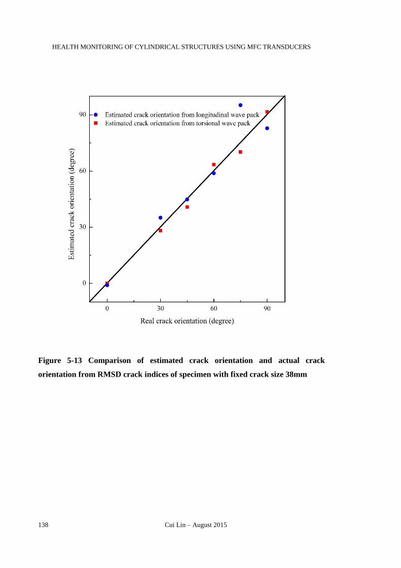
HEALTH MONITORING OF CYLINDRICAL STRUCTURES USING MFC TRANSDUCERS
138 Cui Lin – August 2015
Figure 5-13 Comparison of estimated crack orientation and actual crack
orientation from RMSD crack indices of specimen with fixed crack size 38mm
Chapter 5: The Identification of Crack Orientation and Dimension on Cylindrical Structure
Cui Lin – August 2015 139
5.4.3 Analysis of results
Both numerical simulation results and experimental results verified that the proposed
method is capable of detecting the orientation and dimension of existing line crack on
cylindrical structures. However, some of the facts need to be noted:
1.) The numerical simulation results show better linear pattern than the experimental
data.
This statement is because only full actuation is considered in the numerical simulation
and under such actuation, only axisymmetric wave modes are generated. However, in
the experiment, the MFC patches can only cover part of the circumference of the pipe
where flexural wave modes are also generated. The existence of flexural wave modes
lowered the sensibility of axisymmetric wave modes which increased the uncertainty of
the RMSD value calculated from the wave packs.
2.) The uncertainty of experimental results came from several aspects:
Both the actuator and the sensor are not only covering part of the circumference of the
pipe but also covering part of the pipe in the axial direction, which increased both the
difficulty of identification and the dispersion effect of wave packs.
The results of the experiment are highly sensitive to the quality of the signals especially
the quality of the baseline signals. It is suggested that the baseline signature should be
collected multiple times to ensure the repeatability and stability of the experiment.
3.) Both length and orientation are needed to identify the damage information. When
one parameter is known, the results calculated from Eq.5-2 are quite close to the real
cases as demonstrated in Figure 5-10, Figure 5-12 and Figure 5-13. However, when
both length and orientation of the crack are unknown, more uncertainties arise in the
calculated results. The calculated crack length and direction from the numerical
simulation results and experimental results are listed in and Table 5-4, respectively.

HEALTH MONITORING OF CYLINDRICAL STRUCTURES USING MFC TRANSDUCERS
140 Cui Lin – August 2015
Table 5-3 Estimated crack orientation() and crack length(l) from numerical
simulation
RMSD-T RMSD-L Est. deg Real (deg Est. l(mm) Real l(mm)
0.231496 0.036424 1.81 0 27.8 30
0.365512 0.046202 -0.45 0 44.1 42.5
0.105696 0.053883 29.6 30 12.4 10.68
0.347522 0.190652 33.1 30 40.5 37.38
0.107358 0.067986 41.4 45 12.4 11.34
0.186726 0.140115 55.5 45 21.4 26.46
0.057541 0.045059 60.4 60 6.59 6.16
0.101622 0.081668 64.0 60 11.6 9.24
0.22382 0.191091 75.9 75 25.5 24.876
0.424262 0.359751 74.0 75 48.3 49.752
0.340728 0.296327 82.9 90 38.7 37.38
0.369544 0.319427 80.0 90 42.0 40.05

Chapter 5: The Identification of Crack Orientation and Dimension on Cylindrical Structure
Cui Lin – August 2015 141
Table 5-4 Estimated crack orientation () and crack length(l) from experimental
results
RMSD-T RMSD-L Est. deg Real (deg Est. l (mm) Actual l (mm)
0.306251 0.051177 0.62 0 26.5 28
0.429529 0.076313 2.58 0 37.5 38
0.073626 0.026877 34.1 30 7.5 8
0.188545 0.072998 37.7 30 19.6 23
0.308997 0.131475 44.1 45 33.0 33
0.542132 0.21497 39.2 45 56.6 48
0.213851 0.093079 45.8 60 23.0 18
0.337299 0.172343 60.3 60 38.2 38
0.226077 0.130805 82.7 75 26.8 18
0.376882 0.184674 55.9 75 42.1 43
0.339626 0.200213 90.6 90 40.6 38
0.33336 0.195805 90.5 90 39.8 43
This RMSD crack index method can roughly provide the crack growth trend and detect
its orientation. When simulation model is improved, and advanced signal processing
and mode extraction techniques are adopted in the experiment, more accurate results
can be expected.
5.5 Summary and Conclusion
This chapter presents an RMSD crack index method to identify the crack orientation
and dimension on cylindrical structures. Because of the PM direction of the torsional
wave modes and longitudinal wave modes, the axial crack only has a significant effect
on the transmitted torsional waves, while the circumferential crack affected both
transmitted torsional and longitudinal waves. The RMSD crack index method has been
shown to be able to correlate the RMSD value change of the transmitted wave packs
with the crack growth.

HEALTH MONITORING OF CYLINDRICAL STRUCTURES USING MFC TRANSDUCERS
142 Cui Lin – August 2015
Simplified numerical simulation and experiments have been conducted to verify the
proposed method. The results show that when one parameter is known, the accuracy of
the equations is higher than the case when both parameters are unknown. When both
parameters are unknown, the accuracy of the proposed method is affected. The
improvement of precision may be achieved through the enhancement of the numerical
model or the use of advanced mode extraction technique and an advanced signal
processing technique to remove the effect of flexural waves and noises.

Conclusions and Future Works
Cui Lin – August 2015 143
6 CONCLUSIONS AND FUTURE
WORKS
6.1 Conclusions
This research explored the possibility of using MFC transducers to set up a close-loop
in-situ online SHM system for cylindrical structures. The major contribution of this
research are: 1) use oriented MFC patches to generate torsional wave for axial crack
monitoring of cylindrical structures because of its flexile character and strong
actuating/sensing capacity; 2) use torsional wave RMSD crack index for axial crack
growth monitoring of cylindrical structures; and 3) expand its application to estimate
arbitrary crack dimension and orientation in cylindrical structures.
This study presents a new proposed method that use axisymmetric wave modes for
cylindrical structure SHM.
Firstly, MFC transducers are applied to generate torsional wave for detecting and
monitoring axial direction crack growth in tubular structures. The actuator is driven by
pre-adjusted signals to generate target waveguides for inspection. The sensor picks up
the stress waves propagating in the pipe and returns the electrical signals. With the help
of digital signal processing (DSP) techniques, the damage information is extracted from
the changes of the sensor‘s output. Both numerical and experimental verifications have
been conducted to demonstrate the effectiveness of this method. The results from the
numerical simulation and experimental verification show that the axial-direction crack
propagation can be well monitored. The RMSD values of torsional wave pack from a
numerical simulation with different crack sizes give a linear trend against the crack size
HEALTH MONITORING OF CYLINDRICAL STRUCTURES USING MFC TRANSDUCERS
144 Cui Lin – August 2015
increment. Base on the analysis of both numerical and experimental results, a linear
relationship, can be established between the RMSD value of torsional wave pack and
the axial direction crack size.
Secondly, the SHM system is developed to pick up not only axial crack growth but also
axial crack position. Three pieces of MFC transducers are used in the new regime. The
MFC transducer at the center works as the actuator; the other two MFC transducers
operate as sensors to detect the axial position of the crack and to monitor the crack size
growth, respectively. RMSD crack index is used to monitor the axial crack growth, and
TOF-based method is adopted to find the axial position of the crack in cylindrical
structures. To eliminate the effect of flexural waves, the residual signal whereby the
signal of the undamaged specimen is subtracted from the signal of cracked specimen is
used. Both numerical simulation and experimental investigation are conducted to verify
the proposed method. The results show that both the axial position and crack size
growth of the axial crack can be well located/monitored using this sensing system. In
the experimental investigation, the existence of flexural waves, changes of boundary
conditions, errors in data processing procedure, etc., all contributed to the reduced
accuracy of the results as compared with the numerical simulation. Nevertheless, the
experimental data still show promise in the SHM of axial crack in cylindrical structures.
Finally, based on the RMSD crack index method, an SHM system to identify the crack
orientation and dimension in cylindrical structures are developed. Because of the PM
direction of the T-wave modes and L-wave modes, the axial crack only has a significant
effect on the transmitted T waves, while the circumferential crack affected both the
transmitted T and L waves. The RMSD crack index method has been shown to be able
to correlate the RMSD value change of the transmitted wave packs with the crack
growth. Both numerical simulation and experiments have been conducted to verify the
proposed method. The results show that when one parameter is known, the accuracy of
the equations is higher than the case when both parameters are unknown. When both
parameters are unknown, the accuracy of the proposed method is affected. The
improvement of precision may be achieved through the enhancement of the numerical
model or the use of advanced mode extraction technique and an advanced signal
processing technique to remove the effect of flexural waves and noises.

Conclusions and Future Works
Cui Lin – August 2015 145
From the study performed in this research, we can conclude that using MFC transducers
to carry out SHM for the cylindrical structure is efficient and effective.
6.2 Limitation and Future Works
Compared with other SHM system for cylindrical structures, the system proposed in this
research is compact, easy to setup and with great mobility. It can be moved to anywhere
that the specimen is required to be monitored. It also has the potential to have more
industry applications in the future if below points are addressed.
1. To further develop the proposed system to a close-loop in-situ on-line monitoring,
smart-integrated system.
Figure 6-1 Proposed SHM system for continuous cylindrical structures
Current experiment setup proposed a prototype for the SHM of cylindrical system. As
shown in Figure 6-1, the proposed SHM system can be used for continuous cylindrical
structure monitoring. When crack occurred in region R1, the MFC transducers T1, T2
and T3 will work together as a group. In this group, T1 works as a sensor to pick up
additional wave pack reflected from the crack. T2 works as an actuator and T3 works as
another sensor to collect data to be used for RMSD crack index calculation. Meanwhile,
the system will automatically switch from scanning region R1 to R2. In region R2,
transducers T2, T3 and T4 will work together as a group where T3 as actuator and T2 and
T4 as sensors. The automatic scanning algorithm can be achieved and controlled by the
control unit which can be pre-programed. This proposed system has below benefits:
In-situ monitoring: multiple pieces of transducers are used in the system, and
each of them can monitor its adjacent area;
T T2 T3 T4
R1 R2
Tm Tn

HEALTH MONITORING OF CYLINDRICAL STRUCTURES USING MFC TRANSDUCERS
146 Cui Lin – August 2015
On-line monitoring: real-time monitoring can be achieved since real-time
feedback can be acquired and analysed right away;
Close-loop monitoring: the system can perform SHM by its own, both actuating,
sensing and data processing can be processed by the programmable control unit.
Due to the limitation of equipment and testing specimen, the proposed SHM system for
continuous cylindrical structures is not tested and verified. Implementation work of the
SHM system can be expected in the future.
2. To develop automatic data analysis module
The current data processing procedure requires noise cancellation, RMSD crack index
calculation, curve fitting and other digital signal process techniques if future
information of signal is required. Automatic data analysis module is necessary for the
close-loop monitoring system. The collected data can be automatically processed by the
developed digital signal processing unit. The background noise can be removed from
the signal, and the RMSD crack index as well as the crack location information can be
automatically extracted by the control unit. The development of automatic data analysis
module can also be expected in the author‘s future research plan.
3. More DSP techniques for high resolution crack identification for fatigue type of
cracks
The current experiment study is focusing on the detection of crack induced wave shape
changes on cylindrical structures. With the currently adopted DSP techniques, fracture
types of crack can be well detected and monitored. However, for fatigue type of crack,
the proposed method is not as efficient as it works for fracture types of crack. To
successfully detect and monitor the fatigue type of crack on cylindrical structures,
improved DSP techniques are required to remove the noise from the signal collected
and to extract the useful information from the output signals.
4. Self-powered actuation and signal transmission
Sometimes, an on-line SHM system requires the transducers to be exposed in the
environment that is not accessible to human beings. When the transducer is far from the
control system, it is not practical to use wire to connect all the transducers, especially
when MFC transducers need to be driven by high voltages. It is suggested to use or to
develop a self-powered transducer with wireless signal transmission function.

Conclusions and Future Works
Cui Lin – August 2015 147
5. Bondline effect in numerical simulation
The bondline effect is important in numerical simulation as it will change the output
signal very much. In this study, the bondline of MFC is simplified to a ring type
circle where all nodes on the circle are functioned as actuators. In the experiment, the
MFC transferred the deformation to the epoxy and the epoxy transferred the
deformation to the hosting structure to generate guided waves. Vice versa, similar
reversed process happened at the sensor place. To achieve more accurate SHM results,
the simulation of bondline effect of MFC is necessary
6. The influence of environmental effects like temperature and pressure on the guided
wave propagation.
The proposed experiment setup had been verified both experimentally and numerically.
The verification results had shown its effectiveness to serve the original purpose on
laboratory prepared testing specimen. However, guide wave in tubular structures are
easy to be affected when the environmental condition is changed. For instance, when
the testing temperature is changed, the output signal will also be changed (Codrut,
2014). Since continuous cylindrical structures are often used to transport high
temperature and high pressurized crude oil, it is worth to carry out parametric study on
the effectiveness of proposed testing method. To carry out SHM of cylindrical
structures with high temperature, high pressure fluid in-side, collaboration with
industry partner to carry out on-site SHM experiment on continuous cylindrical
structure is suggested for future works.

HEALTH MONITORING OF CYLINDRICAL STRUCTURES USING MFC TRANSDUCERS
148 Cui Lin – August 2015
REFERENCES
Ahmad, I. (1988). Smart Structures and Materials. U.S. Army Research Office
Workshop on Smart Materials, Structures, and Mathematical Issues. C. A. Rogers.
Virginia Polytechnic Institute & State University, Technomic Publishing Co., Inc: 13-
16.
Alleyne, D. N. and P. Cawley (1992). "Optimization of lamb wave inspection
techniques." NDT & E International 25(1): 11-22.
Alleyne, D. N., M. J. S. Lowe and P. Cawley (1998). "The Reflection of Guided Waves
From Circumferential Notches in Pipes." Journal of Applied Mechanics 65(3): 635-641.
Alleyne, D. N., T. P. Pialucha and P. Cawley (1993). "A signal regeneration technique
for long-range propagation of dispersive Lamb waves." Ultrasonics 31(3): 201-204.
Barshinger, J., J. L. Rose and M. J. Avioli (2002). Guided wave resonance tuning for
pipe inspection. ASME 2002 Pressure Vessels and Piping Conference, American
Society of Mechanical Engineers.
Bhalla, S. and C. Kiong Soh (2003). "Structural impedance based damage diagnosis by
piezo‐transducers." Earthquake engineering & structural dynamics 32(12): 1897-1916.
Bhalla, S., C. K. Soh, K. K. H. Tseng and A. S. K. Naidu (2001). Diagnosis of Incipient
Damage in Steel Structures by Means of Piezoceramic Patches. The 8th East Asia-

References
Cui Lin – August 2015 149
Pacific Conference on Structural Engineering and Construction on Challenges in the
21st Century. Singapore.
Boller, C. (2002). Structural Health Management of Ageing Aircraft and Other
Infrastructure. Monograph on Structural Health Monitoring. Institute of Smart
Structures and Systems (ISSS): 1-59.
Brownjohn, J. M. W., P. Moyo, C. Rizos and T. S. Chuan (2003). Practical Issues in
Using Novel Sensors in SHM of Civil Infrastructure: Problems and Solutions in
Implementation of GPS and Fibre Optics. 4th International Workshop on Structural
health Monitoring: From Diagnostics and Prognostics to Structural Health Management.
F. K. Chang. Stanford University, Stanford, CA, DES Tech Publications Inc.
Çelebi, M. (2000). "GPS in dynamic monitoring of long-period structures." Soil
Dynamics and Earthquake Engineering 20(5–8): 477-483.
Chan, H., et al. (2015). "High frequency guided ultrasonic waves for hidden fatigue
crack growth monitoring in multi-layer model aerospace structures." Smart Materials &
Structures 24(2).
Chang, F.-K. (1997). Structural Health Monitoring: A Summary Report on the First
Stanford Workshop on Structural Health Monitoring.
Cho, H. and C. J. Lissenden (2012). "Structural health monitoring of fatigue crack
growth in plate structures with ultrasonic guided waves." Structural Health Monitoring
11(4): 393-404.
Choi, K. and F. K. Chang (1996). "Identification of impact force and location using
distributed sensors." AIAA Journal 34(1): 136-142.
Codrut Alexandru Dan, Pawel Kudela, Wieslaw Ostachowicz. "Compensation of
Temperature Effects on Guided Wave Based Structural Health Monitoring Systems."
Le Cam, Vincent and Mevel, Laurent and Schoefs, Franck. EWSHM - 7th European
Workshop on Structural Health Monitoring, Jul 2014, Nantes, France. 2014.
Crawley, E. F. and J. De Luis (1987). "Use of piezoelectric actuators as elements of
intelligent structures pages." AIAA Journal 25(10): 1373-1385.
Díaz Valdés, S. H. and C. Soutis (2000). "Health monitoring of composites using Lamb
waves generated by piezoelectric devices." Plastics, Rubber and Composites 29(9): 475-
481.

HEALTH MONITORING OF CYLINDRICAL STRUCTURES USING MFC TRANSDUCERS
150 Cui Lin – August 2015
Demma, A., P. Cawley, M. Lowe and A. G. Roosenbrand (2003). "The reflection of the
fundamental torsional mode from cracks and notches in pipes." The Journal of the
Acoustical Society of America 114(2): 611-625.
Ditri, J. J. and J. L. Rose (1992). "Excitation of guided elastic wave modes in hollow
cylinders by applied surface tractions." Journal of Applied Physics 72(7): 2589-2597.
Ditri, J. J. and J. L. Rose (1993). Generation of guided waves in hollow cylinders by
wedge and comb type transducers. New York, Plenum Press.
Dong, K. and X. Wang (2007). "Wave propagation characteristics in piezoelectric
cylindrical laminated shells under large deformation." Composite structures 77(2): 171-
181.
Esteban, J., F. Lalande and C. A. Rogers (1996). Theoretical modeling of wave
localization due to material damping. 1996 Symposium on Smart Structures and
Materials, International Society for Optics and Photonics.
Farrar, C. R. and D. A. Jauregui (1998). "Comparative study of damage identification
algorithms applied to a bridge: I. Experiment." Smart Materials and Structures 7(5): 704.
Feroz, K. T. and S. O. Oyadiji (1996). Use of PZT sensors for wave propagation studies.
SPIE Smart Structures and Materials1996: Smart Sensing, Processing, and
Instrumentation. K. A. Murphy and D. R. Huston. San Diego. 2718: 36-46.
Fromme, P. and M. B. Sayir (2002). "Measurement of the scattering of a Lamb wave by
a through hole in a plate." The Journal of the Acoustical Society of America 111(3):
1165-1170.
Fugate, M. L., H. Sohn and C. R. Farrar (2001). "VIBRATION-BASED DAMAGE
DETECTION USING STATISTICAL PROCESS CONTROL." Mechanical Systems
and Signal Processing 15(4): 707-721.
Gazis, D. C. (1959a). "Three-Dimensional Investigation of the Propagation of Waves in
Hollow Circular Cylinders. I. Analytical Foundation." The Journal of the Acoustical
Society of America 31(5): 568-573.
Gazis, D. C. (1959b). "Three-Dimensional Investigation of the Propagation of Waves in
Hollow Circular Cylinders. II. Numerical Results." The Journal of the Acoustical
Society of America 31(5): 573-578.

References
Cui Lin – August 2015 151
Ghosh, J. (1923). "Longitudinal vibrations of a hollow cylinder." Bulletin of the
Calcutta Mathematical Society 14: 31-40.
Giurgiutiu, V. (2007). Structural Health Monitoring with Piezoelectric Wafer Active
Sensors, Elsevier.
Giurgiutiu, V. and J. Bao (2004). "Embedded-ultrasonics structural radar for in situ
structural health monitoring of thin-wall structures." Structural Health Monitoring 3(2):
121-140.
Giurgiutiu, V., J. M. Redmond, D. P. Roach and K. Rackow (2000). Active sensors for
health monitoring of aging aerospace structures. SPIE Smart Structures and
Materials2000:Smart Structures and Integrated Systems. N. M. Wereley. San Diego, CA.
3985: 294-305.
Giurgiutiu, V. and C. A. Rogers (1998). Recent advancements in the electromechanical
(E/M) impedance method for structural health monitoring and NDE. SPIE Smart
Structures and Materials 1998: Smart Structures and Integrated Systems,. M. E.
Regelbrugge. San Diego, CA. 3329
Giurgiutiu, V., A. Zagrai and J. Bao (2004). "Damage Identification in Aging Aircraft
Structures with Piezoelectric Wafer Active Sensors." Journal of Intelligent Material
Systems and Structures 15(9-10): 673-687.
Giurgiutiu, V., A. Zagrai and J. J. Bao (2002). "Piezoelectric wafer embedded active
sensors for aging aircraft structural health monitoring." Structural Health Monitoring
1(1): 41-61.
Grondel, S., C. Paget, C. Delebarre, J. Assaad and K. Levin (2002). "Design of optimal
configuration for generating A0 Lamb mode in a composite plate using piezoceramic
transducers." The Journal of the Acoustical Society of America 112(1): 84-90.
Halabe, U. B. and R. Franklin (2001). "Fatigue crack detection in metallic members
using ultrasonic rayleigh waves with time and frequency analyses." Materials
Evaluation 59(3): 424-431.
Harari, A. (1977). "Wave propagation in cylindrical shells with finite regions of
structural discontinuity." The Journal of the Acoustical Society of America 62(5): 1196-
1205.

HEALTH MONITORING OF CYLINDRICAL STRUCTURES USING MFC TRANSDUCERS
152 Cui Lin – August 2015
Hirao, Masahiko, and Hirotsugu Ogi. (1999) "An SH-wave EMAT technique for gas
pipeline inspection." NDT & E International 32, no. 3: 127-132.
IEEE-Standard (1988). "IEEE Standard on Piezoelectricity." ANSI/IEEE Std 176-1987:
0_1.
Jung Y, C., T. Kundu and M. Ehsani (2001). "Internal discontinuity detection in
concrete by lamb waves." Materials Evaluation 59(3): 418-423.
Jim L Cordell(1995) “An Introduction to Conventional and Intelligent Pigging,”
Proceedings of the Pipeline Pigging Conference, 2/13-16, 1995. Cordell, J.L.
Kannan, E., B. Maxfield and K. Balasubramaniam (2007). "SHM of pipes using
torsional waves generated by in situ magnetostrictive tapes." Smart Materials and
Structures 16(6): 2505.
Kawiecki, G. (1998). "Feasibility of Applying Distributed Piezotransducers to
Structural Damage Detection." Journal of Intelligent Material Systems and Structures
9(3): 189-197.
Kessler, S. S., S. M. Spearing, M. J. Atalla, C. E. Cesnik and C. Soutis (2002). "Damage
detection in composite materials using frequency response methods." Composites Part B:
Engineering 33(1): 87-95.
Kim, I.-G., H.-Y. Lee and J.-W. Kim (2005). "Impact damage detection in composite
laminates using PVDF and PZT sensor signals." Journal of intelligent material systems
and structures 16(11-12): 1007-1013.
Kim Y.Y., Park C.I., Cho S.H., Han S.W.(2005) "Torsional wave experiments with a
new magnetostrictive transducer configuration". J. Acoust. Soc. Am.117:3459–3468.
Kim H.W., Lee J.K., Kim Y.Y.(2013) "Circumferential phased array of shear-horizontal
wave magnetostrictive patch transducers for pipe inspection Ultrasonics; 53:423–431
Kuoni, A., R. Holzherr, M. Boillat and N. F. d. Rooij (2003). "Polyimide membrane
with ZnO piezoelectric thin film pressure transducers as a differential pressure liquid
flow sensor." Journal of Micromechanics and Microengineering 13(4): S103.
Le Clézio, E., M. Castaings and B. Hosten (2002). "The interaction of the S0 Lamb
mode with vertical cracks in an aluminium plate." Ultrasonics 40(1–8): 187-192.

References
Cui Lin – August 2015 153
Lee, S. Y., H. J. Nam, Y. S. Kim, W. H. Jin and J. U. Bu (2004). "PZT Cantilevers
Integrated with Heaters and New Piezoelectric Sensors for SPM-Based Nano-Data
Storage Application." Journal of the Korean Physical Society 45(1): 227-230.
Leis, B. "Real time monitoring to detect contact, product loss, and encroachment on
transmission pipelines." In 54 th API Pipeline Conference, April. 2003.
Lestari, W. and P. Qiao (2005). "Application of Wave Propagation Analysis for
Damage Identification in Composite Laminated Beams." Journal of Composite
Materials 39(22): 1967-1984.
Li, J. and J. L. Rose (2001). "Excitation and propagation of non-axisymmetric guided
waves in a hollow cylinder." The Journal of the Acoustical Society of America 109(2):
457-464.
Li, J. and J. L. Rose (2006). "Natural beam focusing of non-axisymmetric guided waves
in large-diameter pipes." Ultrasonics 44(1): 35-45.
Lie Qiu, Shenfang Yuan and Weibo Yang (2014). "On research of time reversal
imaging method and structural health monitoring system." International Journal of
Applied Electromagnetics and Mechanics 46(4):927-941
Lieske, U. and C. Boller (2012). "A view into baseline free guided wave approaches for
structural health monitoring." Structural Health Monitoring 2011. Condition-based
Maintenance and Intelligent Structures. Vol.2 : Proceedings of the Eighth International
Workshop on Structural Health Monitoring; 13.-15.09.2011, Stanford University
Lin, X. and F. Yuan (2001). "Diagnostic Lamb waves in an integrated piezoelectric
sensor/actuator plate: analytical and experimental studies." Smart Materials and
Structures 10(5): 907.
Littlefield, A. G. (2000). Application of the Impedance Method of Modeling Active
Materials to Plate Structures. Doctoral, Rensselaer Polytechnic Institute.
Liu, P., et al. (2014). "Noncontact detection of fatigue cracks by laser nonlinear wave
modulation spectroscopy (LNWMS)." NDT & E International 66(66): 106-116.
Liu, P., et al. (2015). "Baseline-free damage visualization using noncontact laser
nonlinear ultrasonics and state space geometrical changes." Smart Materials &
Structures 24(6).

HEALTH MONITORING OF CYLINDRICAL STRUCTURES USING MFC TRANSDUCERS
154 Cui Lin – August 2015
Maaskant, R., T. Alavie, R. M. Measures, G. Tadros, S. H. Rizkalla and A. Guha-
Thakurta (1997). "Fiber-optic Bragg grating sensors for bridge monitoring." Cement
and Concrete Composites 19(1): 21-33.
Masserey, B. and P. Fromme (2013). "Fatigue crack growth monitoring using high-
frequency guided waves." Structural Health Monitoring 12(5-6): 484-493
Malyarenko, E. V. and M. K. Hinders (2001). "Ultrasonic Lamb wave diffraction
tomography." Ultrasonics 39(4): 269-281.
McKeon, J. C. P. and M. K. Hinders (1999). "LAMB WAVE SCATTERING FROM A
THROUGH HOLE." Journal of Sound and Vibration 224(5): 843-862.
Mustapha, F., G. Manson, K. Worden and S. Pierce (2007). "Damage location in an
isotropic plate using a vector of novelty indices." Mechanical systems and signal
processing 21(4): 1885-1906.
Na, W.-B., T. Kundu and Y.-S. Ryu (2001). "Cylindrical guided waves for inspection of
clay-steel pile interface." KSCE Journal of Civil Engineering 5(1): 29-34.
Naidu, A. S. K. (2004). Structural Damage Identification with Admittance Signature of
Smart PZT Transducer. Doctor of Philosophy thesis, Nanyang Technological University,
Singapore.
Nestleroth, J. B., and T. A. Bubenik(1999). . "Magnetic flux leakage (MFL) technology
for natural gas pipeline inspection." Battelle, Report Number GRI-00/0180 to the Gas
Research Institute
Neumann, D. (1996). "Adaptronik-The Governmental German Activities in the Field of
Smart Structures." Journal of Intelligent Material Systems and Structures 7(2): 246-248.
Ng, S. L., S. C. Tjin, T. Xie and K. T. Soo (1998). "Side-projected fiber-optic velocity
sensors." Photonics Technology Letters, IEEE 10(2): 249-251.
Niethammer, M., L. J. Jacobs, J. Qu and J. Jarzynski (2001). "Time-frequency
representations of Lamb waves." The Journal of the Acoustical Society of America
109(5): 1841-1847.
Okamoto, Jun, Julio C. Adamowski, Marcos SG Tsuzuki, Flávio Buiochi, and Claudio
S. Camerini (1999) "Autonomous system for oil pipelines inspection." Mechatronics 9,
no. 7: 731-743.

References
Cui Lin – August 2015 155
Park, G., H. H. Cudney and D. J. Inman (2000). "Impedance-based health monitoring of
civil structural components." Journal of infrastructure systems 6(4): 153-160.
Park, G., D. J. Inman and C. R. Farrar (2003a). Recent Studies in Piezoelectric
Impedance-Based Structural Health Monitoring. 4th International Workshop on
Structural Health Monitoring: From Diagnostics and Prognostics to Structural Health
Management. F. K. Chang. Stanford, CA,: 1423-1430.
Park, G., H. Sohn, C. R. Farrar and D. J. Inman (2003b). "Overview of Piezoelectric
Impedance-Based Health Monitoring and Path Forward." Shock and Vibration Digest
35(6): 451–463.
Park, J.-S. and J.-H. Kim (2004). "Suppression of aero-thermal large deflections and
snap-through behaviors of composite panels using Macro Fiber Composite actuators."
Smart Materials and Structures 13(6): 1448.
Preumont, A. (2002). Vibration Control of Active Structures: an Introduction.
Dordrecht, Boston and London, Kluwer Academic Publishers.
Qiu, J. and J. Tani (1995). "Vibration Control of a Cylindrical Shell Using Distributed
Piezoelectric Sensors and Actuators." Journal of Intelligent Material Systems and
Structures 6(4): 474-481.
Raja, S., P. K. Sinha, G. Prathap and D. Dwarakanathan (2004). "Influence of active
stiffening on dynamic behaviour of piezo-hygro-thermo-elastic composite plates and
shells." Journal of Sound and Vibration 278(1–2): 257-283.
Reddy, J. N. and J. I. Barbosa (2000). "On vibration suppression of magnetostrictive
beams." Smart Materials and Structures 9(1): 49.
Ritdumrongkul, S., M. Abe, Y. Fujino and T. Miyashita (2004). "Quantitative health
monitoring of bolted joints using a piezoceramic actuator? sensor." Smart Materials and
Structures 13(1): 20.
Ro, J.-J., C.-C. Chien, T.-Y. Wei and S.-J. Sun (2007). "Flexural Vibration Control of
the Circular Handlebars of a Bicycle by Using MFC Actuators." Journal of Vibration
and Control 13(7): 969-987.
Rogers, C. A., D. K. Barker and C. A. Jeger (1988). Introduction to Smart Materials and
Structures. U.S. Army Research Office Workshop on Smart Materials, Structures and

HEALTH MONITORING OF CYLINDRICAL STRUCTURES USING MFC TRANSDUCERS
156 Cui Lin – August 2015
Mathematical Issues. C. A. Rogers. Virginia Polytechnic Institute & State University,
Technomic Publishing Co., Inc: 17-27.
Rose, J. L. (1999). Ultrasonic waves in solid media. U.K., Cambridge University Press.
Rose, J. L., Y. Cho and M. J. Avioli (2009). "Next generation guided wave health
monitoring for long range inspection of pipes." Journal of Loss Prevention in the
Process Industries 22(6): 1010-1015.
Santoni, G. B., L. Yu, B. Xu and V. Giurgiutiu (2007). "Lamb wave-mode tuning of
piezoelectric wafer active sensors for structural health monitoring." Journal of Vibration
and Acoustics 129(6): 752-762.
Satpathi, D., J. P. Victor, M. L. Wang, H. Y. Yang and C. C. Shih (1999). Development
of a PVDF film sensor for infrastructure monitoring. SPIE Smart Structures and
Materials1999: Smart Systems for Bridges, Structures, and Highways. S.-C. Liu.
Newport Beach, CA. 3671: 90-99.
Schönecker, A. J., T. Daue, B. Brückner, C. Freytag, L. Hähne and T. Rödig (2006).
Overview on macro fiber composite applications. SPIE Smart Structures and
Materials2006: Active Materials: Behavior and Mechanics. W. D. Armstrong. San
Diego, CA. 6170: 408-415.
Silk, M. and K. Bainton (1979). "The propagation in metal tubing of ultrasonic wave
modes equivalent to Lamb waves." Ultrasonics 17(1): 11-19.
Sirohi, J. and I. Chopra (2000a). "Fundamental Behavior of Piezoceramic Sheet
Actuators." Journal of Intelligent Material Systems and Structures 11(1): 47-61.
Sirohi, J. and I. Chopra (2000b). "Fundamental Understanding of Piezoelectric Strain
Sensors." Journal of Intelligent Material Systems and Structures 11(4): 246-257.
Sodano, H. A., G. Park and D. J. Inman (2004). "An investigation into the performance
of macro-fiber composites for sensing and structural vibration applications."
Mechanical Systems and Signal Processing 18(3): 683-697.
Stankoff, Alain(1978) "Eddy current generating type metal pipeline detector." U.S.
Patent No. 4,091,322. 23 May 1978.
Stanway, R., J. L. Sproston and A. K. El-Wahed (1996). "Applications of electro-
rheological fluids in vibration control: a survey." Smart Materials and Structures 5(4):
464.

References
Cui Lin – August 2015 157
StorΦy, H., J. SÆther and K. Johannessen (1997). "Fiber Optic Condition Monitoring
during a Full Scale Destructive Bridge Test." Journal of Intelligent Material Systems
and Structures 8(8): 633-643.
Su, Z., L. Ye, X. Bu, X. Wang and Y.-W. Mai (2003). "Quantitative Assessment of
Damage in a Structural Beam Based on Wave Propagation by Impact Excitation."
Structural Health Monitoring 2(1): 27-40.
Sun, F. P., Z. Chaudhry, C. A. Rogers, M. Majmundar and C. Liang (1995). Automated
Real-Time Structure Health Monitoring via Signature Pattern Recognition. SPIE Smart
Structures and Materials 1995: Smart Structures and Integrated Systems. I. Chopra. San
Diego,CA. 2443
Sun, Y., P. Bai, H.-y. Sun and P. Zhou (2005a). "Real-time automatic detection of weld
defects in steel pipe." NDT & E International 38(7): 522-528.
Sun, Z., L. Zhang, B. Gavigan, T. Hayashi and J. L. Rose (2003). "Ultrasonic Flexural
Torsional Guided Wave Pipe Inspection Potential." ASME Conference Proceedings
2003(16974): 29-34.
Sun, Z., L. Zhang and J. L. Rose (2005b). "Flexural-Torsional Guided Wave Mechanics
and Focusing in Pipe." Journal of Pressure Vessel Technology 127(4): 471-478.
Tang, L. and Y. Yang (2012). "A nonlinear piezoelectric energy harvester with
magnetic oscillator." Applied Physics Letters 101(9): 094102-094102-094104.
Tjin, S. C., J. Hao, Y.-Z. Lam, Y. C. Ho and B. K. Ng (2001). "A Pressure Sensor Using
Fiber Bragg Grating." Fiber and Integrated Optics 20(1): 59-69.
Tua, P., S. Quek and Q. Wang (2004). "Detection of cracks in plates using piezo-
actuated Lamb waves." Smart Materials and Structures 13(4): 643.
Tubb, R. (2013). "Pipeline & Gas Journal's 2013 Worldwide Construction Report."
Pipeline & Gas Journal 240(1): 42-54.
Valle, C. and J. W. Littles Jr (2002). "Flaw localization using the reassigned
spectrogram on laser-generated and detected Lamb modes." Ultrasonics 39(8): 535-542.
Viktorov, I. A. (1970). Rayleigh and Lamb waves: physical theory and applications,
Plenum press.

HEALTH MONITORING OF CYLINDRICAL STRUCTURES USING MFC TRANSDUCERS
158 Cui Lin – August 2015
W. Wilkie, J. High and J. Bockman (2002). Reliability Testing of NASA
Piezocomposite Actuators. Proceedings of the Actuator 2002—8th International
Conference on New Actuators, Bremen, Germany.
Wait, J. R., G. Park, H. Sohn and C. R. Farrar (2004). Plate damage identification using
wave propagation and impedance methods. NDE for Health Monitoring and Diagnostics,
International Society for Optics and Photonics.
Wang, G., K. Pran, G. Sagvolden, G. B. Havsgård, A. E. Jensen, G. A. Johnson and S. T.
Vohra (2001). "Ship hull structure monitoring using fibre optic sensors." Smart
Materials and Structures 10(3): 472.
Wang, L. and F. G. Yuan (2005). "Damage Identification in a Composite Plate using
Prestack Reverse-time Migration Technique." Structural Health Monitoring 4(3): 195-
211.
Wang, Y., et al. (2015). "Enhancement of the excitation efficiency of a torsional wave
PPM EMAT array for pipe inspection by optimizing the element number of the array
based on 3-D FEM." Sensors 15(2): 3471-3490.
Wilkie, W. K., R. G. Bryant, J. W. High, R. L. Fox, R. F. Hellbaum, A. J. Jr., B. D.
Little and P. H. Mirick (2000). Low-cost piezo-composite actuator for structural control
applications. SPIE Smart Structures and Materials 2000: Industrial and Commercial
Applications of Smart Structures Technologies. J. H. Jacobs. Newport Beach, CA 3991.
Wu, H., L. Tang, Y. Yang and C. K. Soh (2012). "A novel two-degrees-of-freedom
piezoelectric energy harvester." Journal of Intelligent Material Systems and Structures.
Xu, B. and V. Giurgiutiu (2007). "Single mode tuning effects on Lamb wave time
reversal with piezoelectric wafer active sensors for structural health monitoring."
Journal of Nondestructive Evaluation 26(2-4): 123-134.
Yamakawa, H., H. Iwaki, A. Mita and N. Takeda (1999). Health Monitoring of Steel
Structures Using Fiber Bragg Grating Sensors. 2nd International Workshop on
Structural Health Monitoring. F. K. Chang. Stanford University, Stanford, C.A: 502-
510.
Yuhang, H. (2007). Sensing region of PZT transducers for Structural Health Monitoring.
Master.

References
Cui Lin – August 2015 159
Zhang, X., G. Liu and K. Lam (2001). "Vibration analysis of thin cylindrical shells
using wave propagation approach." Journal of Sound and Vibration 239(3): 397-403.

HEALTH MONITORING OF CYLINDRICAL STRUCTURES USING MFC TRANSDUCERS
160 Cui Lin – August 2015
APPENDIX I LIST OF AUTHOR’S PUBLICATIONS
Lin Cui, Yu Liu, Chee Kiong Soh (2011), "Health monitoring of cylindrical structures
using torsional wave generated by piezoelectric macro-fiber composite", Health
Monitoring of Structural and Biological Systems 2011, Proceedings of SPIE Vol. 7984
(SPIE, Bellingham, WA 2011), 79840G.
Say Ian Lim, Lin Cui, Yu Liu, Chee Kiong Soh (2011), "Monitoring fatigue crack
growth in narrow structural components using Lamb wave technique", Sensors and
Smart Structures Technologies for Civil, Mechanical, and Aerospace Systems 2011,
Proceedings of SPIE Vol. 7981 (SPIE, Bellingham, WA 2011), 798143.
Lin Cui, Say Ian Lim, Miao Shi, Yu Liu, Chee Kiong Soh (2012), "Detection and
monitoring of axial cracks on cylindrical structures using torsional wave generated by
piezoelectric macro-fiber composite", Health Monitoring of Structural and Biological
Systems 2012, Proceedings of SPIE Vol. 8348 (SPIE, Bellingham, WA 2012), 83482N.
Lin Cui, Yu Liu, Chee K Soh (2014), “Macro-fiber composite–based structural health
monitoring system for axial cracks in cylindrical structures”, Journal of Intelligent
Material Systems and Structures, 25(3): 332-341.
Lin Cui, Yu Liu, Chee K Soh (2013), “Identification of crack size and orientation in
continuous cylindrical structure using macro-fiber composite”, Journal of Intelligent
Material Systems and Structures, 25(5):596-605.
Lin Cui, Yu Liu, Say Ian Lim, Chee Kiong Soh (2012), “Crack orientation identification
in continuous cylindrical structure health monitoring using Marco-fiber composite,”
Proc. ASHMCS 2012, CBNU, Jeonju, South Korea.

Appendix II Selected Matlab Codes
Cui Lin – August 2015 161
APPENDIX II SELECTED MATLAB CODES
1. Matlab code to calculate the slope of the RMSD Value
% This is the program for calculating the slope of the RMSD value
% Written by Cui Lin % Date 2012-06-26
% Version 0.1
% Parameter description % m is the number of sets of simulation(node release from 0 to 9)
% n is the number of sets of experiment(crack oriented from 90 to 0).
% k is the number of time steps ocuppied by actuation signal in experiment % or simulation
% l is the window length( the number of time increment in window)
clc;
clear;
m = 8000; n = 12;
a0 = 2;
RMSD = zeros(n,m); crack_length = zeros(n,m);
slope = zeros(n,1);
func=inline('a*x','a','x');
for i = 1:n
slope(i,1) = nlinfit(crack_length(i,:),RMSD(i,:),func,a0); end
clc;
clear;
m = 300;
n = 15;
undamaged_data = zeros(m,1); %need to load from data
damaged_data = zeros(m,n); %need to load from data input = [undamaged_data,damaged_data]; %need to load from data
RMSD= zeros(6,n+1); l = 50;
data_square = zeros(m,n+1);
temp_rmsd_value = zeros(m-l,n+1); rmsd_value = zeros(m-l,n+1);
% calculate the undamaged square data_square(:,1) = input(:,1).^2;
% calculate the RMSD square
for j = 1:n for i = 1:m
data_square(i,j+1) = (input(i,j+1)- input(i,1)).^2;
end end
for i = 1:(m-l) for index = 1:l
temp_rmsd_value(i,1) = temp_rmsd_value(i,1)+ data_square(i+index-1,1);
end for j = 1:n
for index = 1:l
temp_rmsd_value(i,j+1) = temp_rmsd_value(i,j+1)+ data_square(i+index-1,j+1); end
end end
for i = 1:m-l
for j = 1:n rmsd_value(i,j+1) = sqrt(temp_rmsd_value(i,j+1)./temp_rmsd_value(i,1));
end
end

HEALTH MONITORING OF CYLINDRICAL STRUCTURES USING MFC TRANSDUCERS
162 Cui Lin – August 2015
RMSD(1,:) = rmsd_value(111,:);
RMSD(2,:) = rmsd_value(191,:);
RMSD(3,:) = rmsd_value(110,:);
RMSD(4,:) = rmsd_value(190,:);
RMSD(5,:) = rmsd_value(115,:);
RMSD(6,:) = rmsd_value(198,:);
2. Matlab code to generate dispersion curves for phase speed and group speed
% PCDISP Generates dispersion curves for rods & tubes
%
% Last update: 19-1-2011
clear,clc
% ********** USER INPUT DATA **********
% Parameters of the pipe (iron)
c0 = 5040; % bar speed (m/s) nu = .29; % Poisson's ratio
%rho = 7900; % density (kg/m^3)
a = 3.5e-3; % internal radius (m) b = 4e-3; % external radius (m)
% Vector with the circumferential orders to be plotted % The convention is n = -1 for torsional, n = 0 for
% longitudinal, and n >= 1 for flexural
% ex: nvect = [-1 0 1] for T(0,m), L(0,m) and F(1,m) nvect = -1:8;
% Frequency range for the computation fmin = 0; % minimum frequency (Hz)
fmax = 1000e3; % maximum frequency (Hz)
fstep = 10e3; % frequency step (Hz) ftol = 1e-3; % tolerance (for cutoff frequencies) (Hz)
% default = 1 mHz is a good value
% Phase speed range for the computation
cmax = 12000; % maximum phase speed (m/s)
ctol = 1e-3; % tolerance (m/s) % default = 1 mm/s is a good value
% Axes limits for the phase and group speeds plots (m/s) cmin_phase = 0;
cmax_phase = 8000;
cmin_group = 0; cmax_group = 6000;
% Flags for display of phase and group speeds display_phase = 1;
display_group = 1;
display_progress = 1; % small cursor display_speeds = 0; % show the volumetric, rotational & Rayleigh speeds
display_modenames = 1; % displays mode names in the graph (at the end)
% ********** END OF USER INPUT DATA **********
clc disp('PCdisp running')
disp(' ')
tic
gamma = a/b; % gamma = internal/external radii ratio
Nn = length(nvect);
% Scale factors between real and normalized quantities
% sc = (real)/(normalized)
sc_freq = c0/(2*pi*b); % frequency (adim -> Hz)

Appendix II Selected Matlab Codes
Cui Lin – August 2015 163
sc_speed = c0; % speed (adim -> m/s)
% Computes the normalized velocities
[cvolum,crotat,cthinplate,crayleigh]=pcspeeds(nu);
% Creates a color array, in RGB format
% T(0,m) -> red L(0,m) -> blue F(1,m) -> green
% F(n,m) -> shades of green colorvect = [1 0 0; 0 0 1; 0 1 0; .4 .9 0;.3 .8 0; 0.2 .7 0; 0.1 .6 0; 0 .5 0;0 .4 0;0 .3 0;0 .2 0;0 .1 0];
% Cutoff frequencies arrays % (cmax) -> upper cutoff freq (cph = cmax)
% (cinf) -> true cutoff freq (cph = inf)
% length(fcutoff_cinf)>=length(fcutoff_cmax) Nmvect_cmax = zeros(Nn,1);
Nmvect_cinf = zeros(Nn,1);
fcutoff_cmax = []; % upper cutoff frequencies (cph = cmax)
fcutoff_cinf = []; % true cutoff frequencies (cph = inf)
% Find number of branches, compute cutoff frequencies disp('Computing cutoff frequencies...')
disp(' ')
for indn=1:Nn, % Upper axis cutoff frequencies
fcutoff_dummy=pcsolvefreqeqcf(cmax/sc_speed,fmax/sc_freq,ftol/sc_freq,nvect(indn),nu,gamma);
Nmvect_cmax(indn) = length(fcutoff_dummy); fcutoff_cmax(indn,1:length(fcutoff_dummy))=sc_freq*fcutoff_dummy;
% True (cph=inf) cutoff frequencies
fcutoff_dummy=pcsolvefreqeqcf(inf,fmax/sc_freq,ftol/sc_freq,nvect(indn),nu,gamma); Nmvect_cinf(indn) = length(fcutoff_dummy);
fcutoff_cinf(indn,1:length(fcutoff_dummy))=sc_freq*fcutoff_dummy;
if(nvect(indn)==-1), disp('---')
for indm=1:Nmvect_cmax(indn),
disp(sprintf('T(0,%g): cutoff = %g kHz',indm,fcutoff_cmax(indn,indm)/1e3))
end
end if(nvect(indn)==0),
disp('---')
for indm=1:Nmvect_cmax(indn), disp(sprintf('L(0,%g): cutoff = %g kHz',indm,fcutoff_cmax(indn,indm)/1e3))
end
end if(nvect(indn)>0),
disp('---')
for indm=1:Nmvect_cmax(indn), disp(sprintf('F(%g,%g): cutoff = %g kHz',nvect(indn),indm,fcutoff_cmax(indn,indm)/1e3))
end
end end
% Total number of branches that will be plotted
Nbranches = sum(Nmvect_cmax); disp(' ')
disp(sprintf('%g branches will be plotted',Nbranches))
% Creates an "interlaced" array of frequencies, including the
% cutoff frequencies + a little offset
fvect=[pcmkfreqvect(fmin,fmax,fstep) unique(fcutoff_cmax(:))'+fstep/25]; Nf = length(fvect);
% This array will contain the phase speeds % cph = -1 if that frequency is below cutoff for that given mode & branch
cpharray = -ones(Nn,max(Nmvect_cmax),Nf);
% ********** MAIN LOOP (here we go!) **********
disp(' ')
for indf=1:Nf,
f = fvect(indf); disp(sprintf('Computing roots for frequency f = %g kHz (%g%% done)',f/1e3,round(indf/Nf*100)))

HEALTH MONITORING OF CYLINDRICAL STRUCTURES USING MFC TRANSDUCERS
164 Cui Lin – August 2015
for indn = 1:Nn,
n = nvect(indn); disp('---')
disp(sprintf('n = %g',n))
% Find number of roots to be computed
Nrootscomputed=length(find(f>fcutoff_cmax(indn,1:Nmvect_cmax(indn))));
if (Nrootscomputed>0),
cph_tmp = sc_speed*pcsolvefreqeqfc(f/sc_freq,cmax/sc_speed,...
ctol/sc_speed,n,nu,gamma,Nrootscomputed); disp(sprintf('Found %g of %g roots',length(cph_tmp),Nrootscomputed))
% Update the roots array
if (length(cph_tmp)>0), cpharray(indn,1:length(cph_tmp),indf) = cph_tmp';
end
else,
disp(sprintf('No roots found for n = %g and f = %g kHz',n,f/1e3))
end
end
% Let's do the plots
if (display_phase==1), figure(1),clf
axis([fmin/1e3 fmax/1e3 cmin_phase cmax_phase])
xlabel('Frequency (kHz)') ylabel('Phase speed (m/s)')
title('Dispersion curves (phase speed)')
set(gca,'Box','on') %grid on
hold on
end if (display_group==1),
figure(2),clf
axis([fmin/1e3 fmax/1e3 cmin_group cmax_group])
xlabel('Frequency (kHz)')
ylabel('Group speed (m/s)') title('Dispersion curves (group speed)')
set(gca,'Box','on')
%grid on hold on
end
% First we sort the arrays in ascending frequency order
[fvectsort,sortind] = sort(fvect(1:indf));
cpharraysort = cpharray(:,:,sortind); % Update the plots
for indn=1:Nn,
for indm=1:Nmvect_cmax(indn), indplot=find(squeeze(cpharraysort(indn,indm,:))~=-1);
fplotvect=fvectsort(indplot);
cphplotvect=squeeze(cpharraysort(indn,indm,indplot));
% Update phase speed plot
if (length(fplotvect)>0 & display_phase==1), figure(1),plot(fplotvect/1e3,cphplotvect,'Color',colorvect(nvect(indn)+2,:))
end
fgplotvect=[]; cgplotvect=[];
for indfg=2:length(fplotvect),
fgplotvect(indfg-1)=(fplotvect(indfg-1)+fplotvect(indfg))/2; cgplotvect(indfg-1)=(cphplotvect(indfg-1)+cphplotvect(indfg))^2*...
(fplotvect(indfg)-fplotvect(indfg-1))/4/...
(cphplotvect(indfg-1)*fplotvect(indfg)-cphplotvect(indfg)*fplotvect(indfg-1)); end
% Update group speed plot
if (length(fgplotvect)>0 & display_group==1), figure(2),plot(fgplotvect/1e3,cgplotvect,'Color',colorvect(nvect(indn)+2,:))
end
% Place tags with the mode names if (display_modenames==1 & indf==Nf & display_phase==1),
figure(1),

Appendix II Selected Matlab Codes
Cui Lin – August 2015 165
indtag=ceil(rand*length(fplotvect));
text(fplotvect(indtag)/1e3,cphplotvect(indtag),pcmodename(nvect(indn),indm),... 'Color',colorvect(nvect(indn)+2,:));
end
if (display_modenames==1 & indf==Nf & display_group==1), figure(2),
indtag=ceil(rand*length(fgplotvect));
text(fgplotvect(indtag)/1e3,cgplotvect(indtag),pcmodename(nvect(indn),indm),... 'Color',colorvect(nvect(indn)+2,:));
end
end % loop over m end % loop over n
if (display_speeds==1 & display_phase==1), figure(1),
plot([0 fmax]/1e3,cvolum*sc_speed*ones(1,2),'k--')
plot([0 fmax]/1e3,crotat*sc_speed*ones(1,2),'k--')
plot([0 fmax]/1e3,crayleigh*sc_speed*ones(1,2),'k--')
end
if (display_speeds==1 & display_group==1),
figure(2),
plot([0 fmax]/1e3,cvolum*sc_speed*ones(1,2),'k--') plot([0 fmax]/1e3,crotat*sc_speed*ones(1,2),'k--')
plot([0 fmax]/1e3,crayleigh*sc_speed*ones(1,2),'k--')
end
if(display_progress==1 & display_phase==1 & indf<Nf),
figure(1),plot(f/1e3,cmin_phase,'k^') end
if(display_progress==1 & display_group==1 & indf<Nf), figure(2),plot(f/1e3,cmin_group,'k^')
end
drawnow
disp('******************************************')
drawnow
end % End of frequency loop
fvect = fvectsort;
cpharray = cpharraysort;
toc

HEALTH MONITORING OF CYLINDRICAL STRUCTURES USING MFC TRANSDUCERS
166 Cui Lin – August 2015
APPENDIX III SELECTED ANSYS INPUT FILES
1. Undamaged specimen (100 kHz actuation)
/filname,20110724-1
!Start new log, error, lock, and page files /TITLE, shell 100K full actuation NRM undamaged
!Numbers of substeps allowed FINISH
/PREP7
!-----------------------------------------------------------! !Geometry Dimensions !
!-----------------------------------------------------------!
!Alumnium Pipe *SET,pipeL , 1.2
*SET,pipeT , 0.003
*SET,pipeR , 0.0495 *SET,INNRAD , 0.048
*SET,OUTRAD , 0.051
*SET,PL,1.2 !m Length (height) of the pipe
*SET,Ri,0.048 !m Inner radius of the pipe
*SET,Ro,0.051 !m Outer radius of the pipe *SET,RM,0.0495 !m Mid-layer radius of the pipe
*SET,PT,0.003 !m pipe thickness
*SET,ML,0.04 !m lenth of the MFC functional area *SET,MW,0.01 !m width of the MFC functional area
*SET,MT,0.00025 !m thickness of MFC functional area
*SET,Ra,45 !degree deg angle of the MFC sticking on the outer surface of the pipe *SET,RA,Ra*acos(-1)/180 !convert the angle from deg to rad
*SET,POFFS1,0.32 !m location of the Actuator MFC sticking on the pipe from the left end.
*SET,POFFS2,0.9-(ML+MW)*sin(RA) !m location of the Sensor MFC sticking on the pipe from the left end.
*SET,POFFS3,0.6 !m crack starting position
*SET,POFFS4,0.87 !m location of the Sensor
!Piezo and Expoy Offset from the free end of the tube *SET,OffsetX , 0.20
! - Element type !
ET,1,shell63 !Aluminum shell Element
! ! - Material properties
!
MP,DENS,1,2715 !Aluminum density, kg/m^3 MP,EX,1,68e9 !Aluminum Young's modulus, N/m^2
MP,PRXY,1,0.33 !Aluminum Poisson's ratio
R,1,pipeT,pipeT,pipeT,pipeT, , , !Real constant of shell element, thickness at point i,j,k,l RMORE, , , ,
RMORE
RMORE, , !-----------------------------------------------------------!
!FEM Domain Geometries !
!-----------------------------------------------------------! K,1,0,0,0
K,2,0,0,pipeL
!create circle at center 1, radius pipeR Circle,1,pipeR,,,180
lcomb,1,2,0
LSYMM,Y,1 L,1,2
!Drag arc line 1,2,along straght line 3 to create area 1,2
ADRAG,1,,,,,,3 ADRAG,2,,,,,,3
!delete line 3
LDELE, 3 FLST,5,2,5,ORDE,2
FITEM,5,1
FITEM,5,2 ASEL,S, , ,P51X

Appendix III Selected ANSYS INPUT FILES
Cui Lin – August 2015 167
AAtt, 1,1,1,
FLST,5,4,4,ORDE,4 FITEM,5,5
FITEM,5,-6
FITEM,5,8 FITEM,5,-9
CM,_Y,LINE
LSEL, , , ,P51X CM,_Y1,LINE
CMSEL,,_Y
!* LESIZE,_Y1, , ,480, , , , ,1
!*
FLST,5,4,4,ORDE,4 FITEM,5,1
FITEM,5,-2
FITEM,5,4
FITEM,5,7
CM,_Y,LINE
LSEL, , , ,P51X CM,_Y1,LINE
CMSEL,,_Y
!* LESIZE,_Y1, , ,60, , , , ,1
!*
MSHAPE,0,2D MSHKEY,1
!*
FLST,5,2,5,ORDE,2 FITEM,5,1
FITEM,5,-2
CM,_Y,AREA ASEL, , , ,P51X
CM,_Y1,AREA
CHKMSH,'AREA'
CMSEL,S,_Y
!* AMESH,_Y1
!*
CMDELE,_Y CMDELE,_Y1
CMDELE,_Y2
!* Nummrg,node,1e-4
nummrg,kp
allsel,all csys,1
Nrotat,all
EQSLV,SPARSE !Use Sparse matrix solver DMPRAT,0.00 !Define 2% damping ratio
ANTYPE,TRANS !Perform Transient Analysis
!* TRNOPT,FULL
LUMPM,0
!* NSUBST,300,0,0
OUTRES,ERASE
OUTRES,NSOL,1 OUTRES,EPEL,1
TIME,0.0003
FINISH /SOLU
*DEL,_FNCNAME
*DEL,_FNCMTID *DEL,_FNCCSYS
*SET,_FNCNAME,'moment'
*SET,_FNCCSYS,0 ! /INPUT,100K moment.func,,,1
*DIM,%_FNCNAME%,TABLE,6,32,3,,,,%_FNCCSYS%
! ! Begin of equation: {TIME}
*SET,%_FNCNAME%(0,0,1), 0.0, -999

HEALTH MONITORING OF CYLINDRICAL STRUCTURES USING MFC TRANSDUCERS
168 Cui Lin – August 2015
*SET,%_FNCNAME%(2,0,1), 0.0
*SET,%_FNCNAME%(3,0,1), 0.0 *SET,%_FNCNAME%(4,0,1), 0.0
*SET,%_FNCNAME%(5,0,1), 0.0
*SET,%_FNCNAME%(6,0,1), 0.0 *SET,%_FNCNAME%(0,1,1), 1.0, 99, 0, 1, 1, 0, 0
*SET,%_FNCNAME%(0,2,1), 0
*SET,%_FNCNAME%(0,3,1), 0 *SET,%_FNCNAME%(0,4,1), 0
*SET,%_FNCNAME%(0,5,1), 0
*SET,%_FNCNAME%(0,6,1), 0 *SET,%_FNCNAME%(0,7,1), 0
*SET,%_FNCNAME%(0,8,1), 0
*SET,%_FNCNAME%(0,9,1), 0 *SET,%_FNCNAME%(0,10,1), 0
*SET,%_FNCNAME%(0,11,1), 0
*SET,%_FNCNAME%(0,12,1), 0
*SET,%_FNCNAME%(0,13,1), 0
*SET,%_FNCNAME%(0,14,1), 0
*SET,%_FNCNAME%(0,15,1), 0 *SET,%_FNCNAME%(0,16,1), 0
*SET,%_FNCNAME%(0,17,1), 0
*SET,%_FNCNAME%(0,18,1), 0 *SET,%_FNCNAME%(0,19,1), 0
*SET,%_FNCNAME%(0,20,1), 0
*SET,%_FNCNAME%(0,21,1), 0 *SET,%_FNCNAME%(0,22,1), 0
*SET,%_FNCNAME%(0,23,1), 0
*SET,%_FNCNAME%(0,24,1), 0 *SET,%_FNCNAME%(0,25,1), 0
*SET,%_FNCNAME%(0,26,1), 0
*SET,%_FNCNAME%(0,27,1), 0 *SET,%_FNCNAME%(0,28,1), 0
*SET,%_FNCNAME%(0,29,1), 0
*SET,%_FNCNAME%(0,30,1), 0
*SET,%_FNCNAME%(0,31,1), 0
*SET,%_FNCNAME%(0,32,1), 0 ! End of equation: {TIME}
!
! Begin of equation: 1.5*0.5*(1-cos(2*{PI}*{TIME}/5/10^-5))*sin(2*{PI}*10^5* ! {TIME})
*SET,%_FNCNAME%(0,0,2), 0.00005, -999
*SET,%_FNCNAME%(2,0,2), 0.0 *SET,%_FNCNAME%(3,0,2), 0.0
*SET,%_FNCNAME%(4,0,2), 0.0
*SET,%_FNCNAME%(5,0,2), 0.0 *SET,%_FNCNAME%(6,0,2), 0.0
*SET,%_FNCNAME%(0,1,2), 1.0, -1, 0, 1.5, 0, 0, 0
*SET,%_FNCNAME%(0,2,2), 0.0, -2, 0, 0.5, 0, 0, -1 *SET,%_FNCNAME%(0,3,2), 0, -3, 0, 1, -1, 3, -2
*SET,%_FNCNAME%(0,4,2), 0.0, -1, 0, 2, 0, 0, 0
*SET,%_FNCNAME%(0,5,2), 0.0, -2, 0, 3.14159265358979310, 0, 0, -1 *SET,%_FNCNAME%(0,6,2), 0.0, -4, 0, 1, -1, 3, -2
*SET,%_FNCNAME%(0,7,2), 0.0, -1, 0, 1, -4, 3, 1
*SET,%_FNCNAME%(0,8,2), 0.0, -2, 0, 5, 0, 0, -1 *SET,%_FNCNAME%(0,9,2), 0.0, -4, 0, 1, -1, 4, -2
*SET,%_FNCNAME%(0,10,2), 0.0, -1, 0, 0, 0, 0, 0
*SET,%_FNCNAME%(0,11,2), 0.0, -2, 0, 1, 0, 0, -1 *SET,%_FNCNAME%(0,12,2), 0.0, -5, 0, 1, -1, 2, -2
*SET,%_FNCNAME%(0,13,2), 0.0, -1, 0, 5, 0, 0, -5
*SET,%_FNCNAME%(0,14,2), 0.0, -2, 0, 1, -5, 3, -1 *SET,%_FNCNAME%(0,15,2), 0.0, -1, 0, 10, 0, 0, -2
*SET,%_FNCNAME%(0,16,2), 0.0, -5, 0, 1, -1, 17, -2
*SET,%_FNCNAME%(0,17,2), 0.0, -1, 0, 1, -4, 4, -5 *SET,%_FNCNAME%(0,18,2), 0.0, -1, 10, 1, -1, 0, 0
*SET,%_FNCNAME%(0,19,2), 0.0, -2, 0, 1, 0, 0, -1
*SET,%_FNCNAME%(0,20,2), 0.0, -4, 0, 1, -2, 2, -1 *SET,%_FNCNAME%(0,21,2), 0.0, -1, 0, 1, -3, 3, -4
*SET,%_FNCNAME%(0,22,2), 0.0, -2, 0, 2, 0, 0, 0
*SET,%_FNCNAME%(0,23,2), 0.0, -3, 0, 3.14159265358979310, 0, 0, -2 *SET,%_FNCNAME%(0,24,2), 0.0, -4, 0, 1, -2, 3, -3
*SET,%_FNCNAME%(0,25,2), 0.0, -2, 0, 10, 0, 0, 0

Appendix III Selected ANSYS INPUT FILES
Cui Lin – August 2015 169
*SET,%_FNCNAME%(0,26,2), 0.0, -3, 0, 5, 0, 0, -2
*SET,%_FNCNAME%(0,27,2), 0.0, -5, 0, 1, -2, 17, -3 *SET,%_FNCNAME%(0,28,2), 0.0, -2, 0, 1, -4, 3, -5
*SET,%_FNCNAME%(0,29,2), 0.0, -3, 0, 1, -2, 3, 1
*SET,%_FNCNAME%(0,30,2), 0.0, -2, 9, 1, -3, 0, 0 *SET,%_FNCNAME%(0,31,2), 0.0, -3, 0, 1, -1, 3, -2
*SET,%_FNCNAME%(0,32,2), 0.0, 99, 0, 1, -3, 0, 0
! End of equation: 1.5*0.5*(1-cos(2*{PI}*{TIME}/5/10^-5))*sin(2*{PI}*10^5* ! {TIME})
!
! Begin of equation: 0*{TIME} *SET,%_FNCNAME%(0,0,3), 0.001, -999
*SET,%_FNCNAME%(2,0,3), 0.0
*SET,%_FNCNAME%(3,0,3), 0.0 *SET,%_FNCNAME%(4,0,3), 0.0
*SET,%_FNCNAME%(5,0,3), 0.0
*SET,%_FNCNAME%(6,0,3), 0.0
*SET,%_FNCNAME%(0,1,3), 1.0, -1, 0, 0, 0, 0, 1
*SET,%_FNCNAME%(0,2,3), 0.0, -2, 0, 1, -1, 3, 1
*SET,%_FNCNAME%(0,3,3), 0, 99, 0, 1, -2, 0, 0 *SET,%_FNCNAME%(0,4,3), 0
*SET,%_FNCNAME%(0,5,3), 0
*SET,%_FNCNAME%(0,6,3), 0 *SET,%_FNCNAME%(0,7,3), 0
*SET,%_FNCNAME%(0,8,3), 0
*SET,%_FNCNAME%(0,9,3), 0 *SET,%_FNCNAME%(0,10,3), 0
*SET,%_FNCNAME%(0,11,3), 0
*SET,%_FNCNAME%(0,12,3), 0 *SET,%_FNCNAME%(0,13,3), 0
*SET,%_FNCNAME%(0,14,3), 0
*SET,%_FNCNAME%(0,15,3), 0 *SET,%_FNCNAME%(0,16,3), 0
*SET,%_FNCNAME%(0,17,3), 0
*SET,%_FNCNAME%(0,18,3), 0
*SET,%_FNCNAME%(0,19,3), 0
*SET,%_FNCNAME%(0,20,3), 0 *SET,%_FNCNAME%(0,21,3), 0
*SET,%_FNCNAME%(0,22,3), 0
*SET,%_FNCNAME%(0,23,3), 0 *SET,%_FNCNAME%(0,24,3), 0
*SET,%_FNCNAME%(0,25,3), 0
*SET,%_FNCNAME%(0,26,3), 0 *SET,%_FNCNAME%(0,27,3), 0
*SET,%_FNCNAME%(0,28,3), 0
*SET,%_FNCNAME%(0,29,3), 0 *SET,%_FNCNAME%(0,30,3), 0
*SET,%_FNCNAME%(0,31,3), 0
*SET,%_FNCNAME%(0,32,3), 0 ! End of equation: 0*{TIME}
!-->
*DEL,_FNCNAME
*DEL,_FNCMTID
*DEL,_FNCCSYS *SET,_FNCNAME,'force'
*SET,_FNCCSYS,0
! /INPUT,100KHz.func,,,1 *DIM,%_FNCNAME%,TABLE,6,32,3,,,,%_FNCCSYS%
!
! Begin of equation: {TIME} *SET,%_FNCNAME%(0,0,1), 0.0, -999
*SET,%_FNCNAME%(2,0,1), 0.0
*SET,%_FNCNAME%(3,0,1), 0.0 *SET,%_FNCNAME%(4,0,1), 0.0
*SET,%_FNCNAME%(5,0,1), 0.0
*SET,%_FNCNAME%(6,0,1), 0.0 *SET,%_FNCNAME%(0,1,1), 1.0, 99, 0, 1, 1, 0, 0
*SET,%_FNCNAME%(0,2,1), 0
*SET,%_FNCNAME%(0,3,1), 0 *SET,%_FNCNAME%(0,4,1), 0
*SET,%_FNCNAME%(0,5,1), 0

HEALTH MONITORING OF CYLINDRICAL STRUCTURES USING MFC TRANSDUCERS
170 Cui Lin – August 2015
*SET,%_FNCNAME%(0,6,1), 0
*SET,%_FNCNAME%(0,7,1), 0 *SET,%_FNCNAME%(0,8,1), 0
*SET,%_FNCNAME%(0,9,1), 0
*SET,%_FNCNAME%(0,10,1), 0 *SET,%_FNCNAME%(0,11,1), 0
*SET,%_FNCNAME%(0,12,1), 0
*SET,%_FNCNAME%(0,13,1), 0 *SET,%_FNCNAME%(0,14,1), 0
*SET,%_FNCNAME%(0,15,1), 0
*SET,%_FNCNAME%(0,16,1), 0 *SET,%_FNCNAME%(0,17,1), 0
*SET,%_FNCNAME%(0,18,1), 0
*SET,%_FNCNAME%(0,19,1), 0 *SET,%_FNCNAME%(0,20,1), 0
*SET,%_FNCNAME%(0,21,1), 0
*SET,%_FNCNAME%(0,22,1), 0
*SET,%_FNCNAME%(0,23,1), 0
*SET,%_FNCNAME%(0,24,1), 0
*SET,%_FNCNAME%(0,25,1), 0 *SET,%_FNCNAME%(0,26,1), 0
*SET,%_FNCNAME%(0,27,1), 0
*SET,%_FNCNAME%(0,28,1), 0 *SET,%_FNCNAME%(0,29,1), 0
*SET,%_FNCNAME%(0,30,1), 0
*SET,%_FNCNAME%(0,31,1), 0 *SET,%_FNCNAME%(0,32,1), 0
! End of equation: {TIME}
! ! Begin of equation: 1000*0.5*(1-cos(2*{PI}*{TIME}/5/10^-5))*sin(2*{PI}*10^5*
! {TIME})
*SET,%_FNCNAME%(0,0,2), 0.00005, -999 *SET,%_FNCNAME%(2,0,2), 0.0
*SET,%_FNCNAME%(3,0,2), 0.0
*SET,%_FNCNAME%(4,0,2), 0.0
*SET,%_FNCNAME%(5,0,2), 0.0
*SET,%_FNCNAME%(6,0,2), 0.0 *SET,%_FNCNAME%(0,1,2), 1.0, -1, 0, 1000, 0, 0, 0
*SET,%_FNCNAME%(0,2,2), 0.0, -2, 0, 0.5, 0, 0, -1
*SET,%_FNCNAME%(0,3,2), 0, -3, 0, 1, -1, 3, -2 *SET,%_FNCNAME%(0,4,2), 0.0, -1, 0, 2, 0, 0, 0
*SET,%_FNCNAME%(0,5,2), 0.0, -2, 0, 3.14159265358979310, 0, 0, -1
*SET,%_FNCNAME%(0,6,2), 0.0, -4, 0, 1, -1, 3, -2 *SET,%_FNCNAME%(0,7,2), 0.0, -1, 0, 1, -4, 3, 1
*SET,%_FNCNAME%(0,8,2), 0.0, -2, 0, 5, 0, 0, -1
*SET,%_FNCNAME%(0,9,2), 0.0, -4, 0, 1, -1, 4, -2 *SET,%_FNCNAME%(0,10,2), 0.0, -1, 0, 0, 0, 0, 0
*SET,%_FNCNAME%(0,11,2), 0.0, -2, 0, 1, 0, 0, -1
*SET,%_FNCNAME%(0,12,2), 0.0, -5, 0, 1, -1, 2, -2 *SET,%_FNCNAME%(0,13,2), 0.0, -1, 0, 5, 0, 0, -5
*SET,%_FNCNAME%(0,14,2), 0.0, -2, 0, 1, -5, 3, -1
*SET,%_FNCNAME%(0,15,2), 0.0, -1, 0, 10, 0, 0, -2 *SET,%_FNCNAME%(0,16,2), 0.0, -5, 0, 1, -1, 17, -2
*SET,%_FNCNAME%(0,17,2), 0.0, -1, 0, 1, -4, 4, -5
*SET,%_FNCNAME%(0,18,2), 0.0, -1, 10, 1, -1, 0, 0 *SET,%_FNCNAME%(0,19,2), 0.0, -2, 0, 1, 0, 0, -1
*SET,%_FNCNAME%(0,20,2), 0.0, -4, 0, 1, -2, 2, -1
*SET,%_FNCNAME%(0,21,2), 0.0, -1, 0, 1, -3, 3, -4 *SET,%_FNCNAME%(0,22,2), 0.0, -2, 0, 2, 0, 0, 0
*SET,%_FNCNAME%(0,23,2), 0.0, -3, 0, 3.14159265358979310, 0, 0, -2
*SET,%_FNCNAME%(0,24,2), 0.0, -4, 0, 1, -2, 3, -3 *SET,%_FNCNAME%(0,25,2), 0.0, -2, 0, 10, 0, 0, 0
*SET,%_FNCNAME%(0,26,2), 0.0, -3, 0, 5, 0, 0, -2
*SET,%_FNCNAME%(0,27,2), 0.0, -5, 0, 1, -2, 17, -3 *SET,%_FNCNAME%(0,28,2), 0.0, -2, 0, 1, -4, 3, -5
*SET,%_FNCNAME%(0,29,2), 0.0, -3, 0, 1, -2, 3, 1
*SET,%_FNCNAME%(0,30,2), 0.0, -2, 9, 1, -3, 0, 0 *SET,%_FNCNAME%(0,31,2), 0.0, -3, 0, 1, -1, 3, -2
*SET,%_FNCNAME%(0,32,2), 0.0, 99, 0, 1, -3, 0, 0
! End of equation: 1000*0.5*(1-cos(2*{PI}*{TIME}/5/10^-5))*sin(2*{PI}*10^5* ! {TIME})
!

Appendix III Selected ANSYS INPUT FILES
Cui Lin – August 2015 171
! Begin of equation: 0*{TIME}
*SET,%_FNCNAME%(0,0,3), 0.001, -999 *SET,%_FNCNAME%(2,0,3), 0.0
*SET,%_FNCNAME%(3,0,3), 0.0
*SET,%_FNCNAME%(4,0,3), 0.0 *SET,%_FNCNAME%(5,0,3), 0.0
*SET,%_FNCNAME%(6,0,3), 0.0
*SET,%_FNCNAME%(0,1,3), 1.0, -1, 0, 0, 0, 0, 1 *SET,%_FNCNAME%(0,2,3), 0.0, -2, 0, 1, -1, 3, 1
*SET,%_FNCNAME%(0,3,3), 0, 99, 0, 1, -2, 0, 0
*SET,%_FNCNAME%(0,4,3), 0 *SET,%_FNCNAME%(0,5,3), 0
*SET,%_FNCNAME%(0,6,3), 0
*SET,%_FNCNAME%(0,7,3), 0 *SET,%_FNCNAME%(0,8,3), 0
*SET,%_FNCNAME%(0,9,3), 0
*SET,%_FNCNAME%(0,10,3), 0
*SET,%_FNCNAME%(0,11,3), 0
*SET,%_FNCNAME%(0,12,3), 0
*SET,%_FNCNAME%(0,13,3), 0 *SET,%_FNCNAME%(0,14,3), 0
*SET,%_FNCNAME%(0,15,3), 0
*SET,%_FNCNAME%(0,16,3), 0 *SET,%_FNCNAME%(0,17,3), 0
*SET,%_FNCNAME%(0,18,3), 0
*SET,%_FNCNAME%(0,19,3), 0 *SET,%_FNCNAME%(0,20,3), 0
*SET,%_FNCNAME%(0,21,3), 0
*SET,%_FNCNAME%(0,22,3), 0 *SET,%_FNCNAME%(0,23,3), 0
*SET,%_FNCNAME%(0,24,3), 0
*SET,%_FNCNAME%(0,25,3), 0 *SET,%_FNCNAME%(0,26,3), 0
*SET,%_FNCNAME%(0,27,3), 0
*SET,%_FNCNAME%(0,28,3), 0
*SET,%_FNCNAME%(0,29,3), 0
*SET,%_FNCNAME%(0,30,3), 0 *SET,%_FNCNAME%(0,31,3), 0
*SET,%_FNCNAME%(0,32,3), 0
! End of equation: 0*{TIME} !-->
nsel,s,loc,z,poffs1-1e-8,poffs1+1e-8
f,all,FY,%FORCE%
f,all,FZ,%FORCE% f,all,MY,%MOMENT%
f,all,MZ,%MOMENT%
alls,all nsel,s,loc,z,PL-1e-8,PL+1e-8
d,all,ux,0
d,all,uy,0 d,all,uz,0
d,all,ROTX,0
D,all,ROTY,0 D,all,ROTZ,0
alls,all
finish
/solu
solve
finish
/solu solve
SAVE, 20110724-1,db

HEALTH MONITORING OF CYLINDRICAL STRUCTURES USING MFC TRANSDUCERS
172 Cui Lin – August 2015
2. Specimen with Longitudinal crack (100 kHz actuation)
/filname,20110725-5
!Start new log, error, lock, and page files /TITLE, shell 100K full actuation NRM release 9 nodes cracked
!Numbers of substeps allowed FINISH
/PREP7
!-----------------------------------------------------------! !Geometry Dimensions !
!-----------------------------------------------------------!
!Alumnium Pipe *SET,pipeL , 1.2
*SET,pipeT , 0.003
*SET,pipeR , 0.0495 *SET,INNRAD , 0.048
*SET,OUTRAD , 0.051
*SET,PL,1.2 !m Length (height) of the pipe
*SET,Ri,0.048 !m Inner radius of the pipe
*SET,Ro,0.051 !m Outer radius of the pipe *SET,RM,0.0495 !m Mid-layer radius of the pipe
*SET,PT,0.003 !m pipe thickness
*SET,ML,0.04 !m lenth of the MFC functional area *SET,MW,0.01 !m width of the MFC functional area
*SET,MT,0.00025 !m thickness of MFC functional area
*SET,Ra,45 !degree deg angle of the MFC sticking on the outer surface of the pipe *SET,RA,Ra*acos(-1)/180 !convert the angle from deg to rad
*SET,POFFS1,0.32 !m location of the Actuator MFC sticking on the pipe from the left end.
*SET,POFFS2,0.9-(ML+MW)*sin(RA) !m location of the Sensor MFC sticking on the pipe from the left end. *SET,POFFS3,0.6 !m crack starting position
*SET,POFFS4,0.87 !m location of the Sensor
!Piezo and Expoy Offset from the free end of the tube *SET,OffsetX , 0.20
! - Element type !
ET,1,shell63 !Aluminum shell Element
! ! - Material properties
!
MP,DENS,1,2715 !Aluminum density, kg/m^3 MP,EX,1,68e9 !Aluminum Young's modulus, N/m^2
MP,PRXY,1,0.33 !Aluminum Poisson's ratio
R,1,pipeT,pipeT,pipeT,pipeT, , , !Real constant of shell element, thickness at point i,j,k,l RMORE, , , ,
RMORE
RMORE, , !-----------------------------------------------------------!
!FEM Domain Geometries !
!-----------------------------------------------------------!
K,1,0,0,0
K,2,0,0,pipeL
!create circle at center 1, radius pipeR Circle,1,pipeR,,,180
lcomb,1,2,0
LSYMM,Y,1 L,1,2
!Drag arc line 1,2,along straght line 3 to create area 1,2
ADRAG,1,,,,,,3 ADRAG,2,,,,,,3
!delete line 3
LDELE, 3 FLST,5,2,5,ORDE,2
FITEM,5,1
FITEM,5,2 ASEL,S, , ,P51X
AAtt, 1,1,1,
FLST,5,4,4,ORDE,4

Appendix III Selected ANSYS INPUT FILES
Cui Lin – August 2015 173
FITEM,5,5
FITEM,5,-6 FITEM,5,8
FITEM,5,-9
CM,_Y,LINE LSEL, , , ,P51X
CM,_Y1,LINE
CMSEL,,_Y !*
LESIZE,_Y1, , ,480, , , , ,1
!* FLST,5,4,4,ORDE,4
FITEM,5,1
FITEM,5,-2 FITEM,5,4
FITEM,5,7
CM,_Y,LINE
LSEL, , , ,P51X
CM,_Y1,LINE
CMSEL,,_Y !*
LESIZE,_Y1, , ,60, , , , ,1
!* MSHAPE,0,2D
MSHKEY,1
!* FLST,5,2,5,ORDE,2
FITEM,5,1
FITEM,5,-2 CM,_Y,AREA
ASEL, , , ,P51X
CM,_Y1,AREA CHKMSH,'AREA'
CMSEL,S,_Y
!*
AMESH,_Y1
!* CMDELE,_Y
CMDELE,_Y1
CMDELE,_Y2 !*
NSEL,S,LOC,X,-pipeR-1e-10,-pipeR+1e-10, NUMMRG,NODE,
NSEL,S,LOC,X,pipeR-1e-10,pipeR+1e-10,
NSEL,R,LOC,Z,0,PIPEL/2-0.013 NUMMRG,NODE,
NSEL,S,LOC,X,pipeR-1e-10,pipeR+1e-10,
NSEL,R,LOC,Z,PIPEL/2+0.013,PIPEL NUMMRG,NODE,
allsel,all
csys,1
Nrotat,all EQSLV,SPARSE !Use Sparse matrix solver
DMPRAT,0.00 !Define 2% damping ratio
ANTYPE,TRANS !Perform Transient Analysis !*
TRNOPT,FULL
LUMPM,0 !*
NSUBST,300,0,0
OUTRES,ERASE OUTRES,NSOL,1
OUTRES,EPEL,1
TIME,0.0003 FINISH
/SOLU
*DEL,_FNCNAME *DEL,_FNCMTID
*DEL,_FNCCSYS

HEALTH MONITORING OF CYLINDRICAL STRUCTURES USING MFC TRANSDUCERS
174 Cui Lin – August 2015
*SET,_FNCNAME,'moment'
*SET,_FNCCSYS,0 ! /INPUT,100K moment.func,,,1
*DIM,%_FNCNAME%,TABLE,6,32,3,,,,%_FNCCSYS%
! ! Begin of equation: {TIME}
*SET,%_FNCNAME%(0,0,1), 0.0, -999
*SET,%_FNCNAME%(2,0,1), 0.0 *SET,%_FNCNAME%(3,0,1), 0.0
*SET,%_FNCNAME%(4,0,1), 0.0
*SET,%_FNCNAME%(5,0,1), 0.0 *SET,%_FNCNAME%(6,0,1), 0.0
*SET,%_FNCNAME%(0,1,1), 1.0, 99, 0, 1, 1, 0, 0
*SET,%_FNCNAME%(0,2,1), 0 *SET,%_FNCNAME%(0,3,1), 0
*SET,%_FNCNAME%(0,4,1), 0
*SET,%_FNCNAME%(0,5,1), 0
*SET,%_FNCNAME%(0,6,1), 0
*SET,%_FNCNAME%(0,7,1), 0
*SET,%_FNCNAME%(0,8,1), 0 *SET,%_FNCNAME%(0,9,1), 0
*SET,%_FNCNAME%(0,10,1), 0
*SET,%_FNCNAME%(0,11,1), 0 *SET,%_FNCNAME%(0,12,1), 0
*SET,%_FNCNAME%(0,13,1), 0
*SET,%_FNCNAME%(0,14,1), 0 *SET,%_FNCNAME%(0,15,1), 0
*SET,%_FNCNAME%(0,16,1), 0
*SET,%_FNCNAME%(0,17,1), 0 *SET,%_FNCNAME%(0,18,1), 0
*SET,%_FNCNAME%(0,19,1), 0
*SET,%_FNCNAME%(0,20,1), 0 *SET,%_FNCNAME%(0,21,1), 0
*SET,%_FNCNAME%(0,22,1), 0
*SET,%_FNCNAME%(0,23,1), 0
*SET,%_FNCNAME%(0,24,1), 0
*SET,%_FNCNAME%(0,25,1), 0 *SET,%_FNCNAME%(0,26,1), 0
*SET,%_FNCNAME%(0,27,1), 0
*SET,%_FNCNAME%(0,28,1), 0 *SET,%_FNCNAME%(0,29,1), 0
*SET,%_FNCNAME%(0,30,1), 0
*SET,%_FNCNAME%(0,31,1), 0 *SET,%_FNCNAME%(0,32,1), 0
! End of equation: {TIME}
! ! Begin of equation: 1.5*0.5*(1-cos(2*{PI}*{TIME}/5/10^-5))*sin(2*{PI}*10^5*
! {TIME})
*SET,%_FNCNAME%(0,0,2), 0.00005, -999 *SET,%_FNCNAME%(2,0,2), 0.0
*SET,%_FNCNAME%(3,0,2), 0.0
*SET,%_FNCNAME%(4,0,2), 0.0 *SET,%_FNCNAME%(5,0,2), 0.0
*SET,%_FNCNAME%(6,0,2), 0.0
*SET,%_FNCNAME%(0,1,2), 1.0, -1, 0, 1.5, 0, 0, 0 *SET,%_FNCNAME%(0,2,2), 0.0, -2, 0, 0.5, 0, 0, -1
*SET,%_FNCNAME%(0,3,2), 0, -3, 0, 1, -1, 3, -2
*SET,%_FNCNAME%(0,4,2), 0.0, -1, 0, 2, 0, 0, 0 *SET,%_FNCNAME%(0,5,2), 0.0, -2, 0, 3.14159265358979310, 0, 0, -1
*SET,%_FNCNAME%(0,6,2), 0.0, -4, 0, 1, -1, 3, -2
*SET,%_FNCNAME%(0,7,2), 0.0, -1, 0, 1, -4, 3, 1 *SET,%_FNCNAME%(0,8,2), 0.0, -2, 0, 5, 0, 0, -1
*SET,%_FNCNAME%(0,9,2), 0.0, -4, 0, 1, -1, 4, -2
*SET,%_FNCNAME%(0,10,2), 0.0, -1, 0, 0, 0, 0, 0 *SET,%_FNCNAME%(0,11,2), 0.0, -2, 0, 1, 0, 0, -1
*SET,%_FNCNAME%(0,12,2), 0.0, -5, 0, 1, -1, 2, -2
*SET,%_FNCNAME%(0,13,2), 0.0, -1, 0, 5, 0, 0, -5 *SET,%_FNCNAME%(0,14,2), 0.0, -2, 0, 1, -5, 3, -1
*SET,%_FNCNAME%(0,15,2), 0.0, -1, 0, 10, 0, 0, -2
*SET,%_FNCNAME%(0,16,2), 0.0, -5, 0, 1, -1, 17, -2 *SET,%_FNCNAME%(0,17,2), 0.0, -1, 0, 1, -4, 4, -5
*SET,%_FNCNAME%(0,18,2), 0.0, -1, 10, 1, -1, 0, 0

Appendix III Selected ANSYS INPUT FILES
Cui Lin – August 2015 175
*SET,%_FNCNAME%(0,19,2), 0.0, -2, 0, 1, 0, 0, -1
*SET,%_FNCNAME%(0,20,2), 0.0, -4, 0, 1, -2, 2, -1 *SET,%_FNCNAME%(0,21,2), 0.0, -1, 0, 1, -3, 3, -4
*SET,%_FNCNAME%(0,22,2), 0.0, -2, 0, 2, 0, 0, 0
*SET,%_FNCNAME%(0,23,2), 0.0, -3, 0, 3.14159265358979310, 0, 0, -2 *SET,%_FNCNAME%(0,24,2), 0.0, -4, 0, 1, -2, 3, -3
*SET,%_FNCNAME%(0,25,2), 0.0, -2, 0, 10, 0, 0, 0
*SET,%_FNCNAME%(0,26,2), 0.0, -3, 0, 5, 0, 0, -2 *SET,%_FNCNAME%(0,27,2), 0.0, -5, 0, 1, -2, 17, -3
*SET,%_FNCNAME%(0,28,2), 0.0, -2, 0, 1, -4, 3, -5
*SET,%_FNCNAME%(0,29,2), 0.0, -3, 0, 1, -2, 3, 1 *SET,%_FNCNAME%(0,30,2), 0.0, -2, 9, 1, -3, 0, 0
*SET,%_FNCNAME%(0,31,2), 0.0, -3, 0, 1, -1, 3, -2
*SET,%_FNCNAME%(0,32,2), 0.0, 99, 0, 1, -3, 0, 0 ! End of equation: 1.5*0.5*(1-cos(2*{PI}*{TIME}/5/10^-5))*sin(2*{PI}*10^5*
! {TIME})
!
! Begin of equation: 0*{TIME}
*SET,%_FNCNAME%(0,0,3), 0.001, -999
*SET,%_FNCNAME%(2,0,3), 0.0 *SET,%_FNCNAME%(3,0,3), 0.0
*SET,%_FNCNAME%(4,0,3), 0.0
*SET,%_FNCNAME%(5,0,3), 0.0 *SET,%_FNCNAME%(6,0,3), 0.0
*SET,%_FNCNAME%(0,1,3), 1.0, -1, 0, 0, 0, 0, 1
*SET,%_FNCNAME%(0,2,3), 0.0, -2, 0, 1, -1, 3, 1 *SET,%_FNCNAME%(0,3,3), 0, 99, 0, 1, -2, 0, 0
*SET,%_FNCNAME%(0,4,3), 0
*SET,%_FNCNAME%(0,5,3), 0 *SET,%_FNCNAME%(0,6,3), 0
*SET,%_FNCNAME%(0,7,3), 0
*SET,%_FNCNAME%(0,8,3), 0 *SET,%_FNCNAME%(0,9,3), 0
*SET,%_FNCNAME%(0,10,3), 0
*SET,%_FNCNAME%(0,11,3), 0
*SET,%_FNCNAME%(0,12,3), 0
*SET,%_FNCNAME%(0,13,3), 0 *SET,%_FNCNAME%(0,14,3), 0
*SET,%_FNCNAME%(0,15,3), 0
*SET,%_FNCNAME%(0,16,3), 0 *SET,%_FNCNAME%(0,17,3), 0
*SET,%_FNCNAME%(0,18,3), 0
*SET,%_FNCNAME%(0,19,3), 0 *SET,%_FNCNAME%(0,20,3), 0
*SET,%_FNCNAME%(0,21,3), 0
*SET,%_FNCNAME%(0,22,3), 0 *SET,%_FNCNAME%(0,23,3), 0
*SET,%_FNCNAME%(0,24,3), 0
*SET,%_FNCNAME%(0,25,3), 0 *SET,%_FNCNAME%(0,26,3), 0
*SET,%_FNCNAME%(0,27,3), 0
*SET,%_FNCNAME%(0,28,3), 0 *SET,%_FNCNAME%(0,29,3), 0
*SET,%_FNCNAME%(0,30,3), 0
*SET,%_FNCNAME%(0,31,3), 0 *SET,%_FNCNAME%(0,32,3), 0
! End of equation: 0*{TIME}
!-->
*DEL,_FNCNAME
*DEL,_FNCMTID *DEL,_FNCCSYS
*SET,_FNCNAME,'force'
*SET,_FNCCSYS,0 ! /INPUT,100KHz.func,,,1
*DIM,%_FNCNAME%,TABLE,6,32,3,,,,%_FNCCSYS%
! ! Begin of equation: {TIME}
*SET,%_FNCNAME%(0,0,1), 0.0, -999
*SET,%_FNCNAME%(2,0,1), 0.0 *SET,%_FNCNAME%(3,0,1), 0.0
*SET,%_FNCNAME%(4,0,1), 0.0

HEALTH MONITORING OF CYLINDRICAL STRUCTURES USING MFC TRANSDUCERS
176 Cui Lin – August 2015
*SET,%_FNCNAME%(5,0,1), 0.0
*SET,%_FNCNAME%(6,0,1), 0.0 *SET,%_FNCNAME%(0,1,1), 1.0, 99, 0, 1, 1, 0, 0
*SET,%_FNCNAME%(0,2,1), 0
*SET,%_FNCNAME%(0,3,1), 0 *SET,%_FNCNAME%(0,4,1), 0
*SET,%_FNCNAME%(0,5,1), 0
*SET,%_FNCNAME%(0,6,1), 0 *SET,%_FNCNAME%(0,7,1), 0
*SET,%_FNCNAME%(0,8,1), 0
*SET,%_FNCNAME%(0,9,1), 0 *SET,%_FNCNAME%(0,10,1), 0
*SET,%_FNCNAME%(0,11,1), 0
*SET,%_FNCNAME%(0,12,1), 0 *SET,%_FNCNAME%(0,13,1), 0
*SET,%_FNCNAME%(0,14,1), 0
*SET,%_FNCNAME%(0,15,1), 0
*SET,%_FNCNAME%(0,16,1), 0
*SET,%_FNCNAME%(0,17,1), 0
*SET,%_FNCNAME%(0,18,1), 0 *SET,%_FNCNAME%(0,19,1), 0
*SET,%_FNCNAME%(0,20,1), 0
*SET,%_FNCNAME%(0,21,1), 0 *SET,%_FNCNAME%(0,22,1), 0
*SET,%_FNCNAME%(0,23,1), 0
*SET,%_FNCNAME%(0,24,1), 0 *SET,%_FNCNAME%(0,25,1), 0
*SET,%_FNCNAME%(0,26,1), 0
*SET,%_FNCNAME%(0,27,1), 0 *SET,%_FNCNAME%(0,28,1), 0
*SET,%_FNCNAME%(0,29,1), 0
*SET,%_FNCNAME%(0,30,1), 0 *SET,%_FNCNAME%(0,31,1), 0
*SET,%_FNCNAME%(0,32,1), 0
! End of equation: {TIME}
!
! Begin of equation: 1000*0.5*(1-cos(2*{PI}*{TIME}/5/10^-5))*sin(2*{PI}*10^5* ! {TIME})
*SET,%_FNCNAME%(0,0,2), 0.00005, -999
*SET,%_FNCNAME%(2,0,2), 0.0 *SET,%_FNCNAME%(3,0,2), 0.0
*SET,%_FNCNAME%(4,0,2), 0.0
*SET,%_FNCNAME%(5,0,2), 0.0 *SET,%_FNCNAME%(6,0,2), 0.0
*SET,%_FNCNAME%(0,1,2), 1.0, -1, 0, 1000, 0, 0, 0
*SET,%_FNCNAME%(0,2,2), 0.0, -2, 0, 0.5, 0, 0, -1 *SET,%_FNCNAME%(0,3,2), 0, -3, 0, 1, -1, 3, -2
*SET,%_FNCNAME%(0,4,2), 0.0, -1, 0, 2, 0, 0, 0
*SET,%_FNCNAME%(0,5,2), 0.0, -2, 0, 3.14159265358979310, 0, 0, -1 *SET,%_FNCNAME%(0,6,2), 0.0, -4, 0, 1, -1, 3, -2
*SET,%_FNCNAME%(0,7,2), 0.0, -1, 0, 1, -4, 3, 1
*SET,%_FNCNAME%(0,8,2), 0.0, -2, 0, 5, 0, 0, -1 *SET,%_FNCNAME%(0,9,2), 0.0, -4, 0, 1, -1, 4, -2
*SET,%_FNCNAME%(0,10,2), 0.0, -1, 0, 0, 0, 0, 0
*SET,%_FNCNAME%(0,11,2), 0.0, -2, 0, 1, 0, 0, -1 *SET,%_FNCNAME%(0,12,2), 0.0, -5, 0, 1, -1, 2, -2
*SET,%_FNCNAME%(0,13,2), 0.0, -1, 0, 5, 0, 0, -5
*SET,%_FNCNAME%(0,14,2), 0.0, -2, 0, 1, -5, 3, -1 *SET,%_FNCNAME%(0,15,2), 0.0, -1, 0, 10, 0, 0, -2
*SET,%_FNCNAME%(0,16,2), 0.0, -5, 0, 1, -1, 17, -2
*SET,%_FNCNAME%(0,17,2), 0.0, -1, 0, 1, -4, 4, -5 *SET,%_FNCNAME%(0,18,2), 0.0, -1, 10, 1, -1, 0, 0
*SET,%_FNCNAME%(0,19,2), 0.0, -2, 0, 1, 0, 0, -1
*SET,%_FNCNAME%(0,20,2), 0.0, -4, 0, 1, -2, 2, -1 *SET,%_FNCNAME%(0,21,2), 0.0, -1, 0, 1, -3, 3, -4
*SET,%_FNCNAME%(0,22,2), 0.0, -2, 0, 2, 0, 0, 0
*SET,%_FNCNAME%(0,23,2), 0.0, -3, 0, 3.14159265358979310, 0, 0, -2 *SET,%_FNCNAME%(0,24,2), 0.0, -4, 0, 1, -2, 3, -3
*SET,%_FNCNAME%(0,25,2), 0.0, -2, 0, 10, 0, 0, 0
*SET,%_FNCNAME%(0,26,2), 0.0, -3, 0, 5, 0, 0, -2 *SET,%_FNCNAME%(0,27,2), 0.0, -5, 0, 1, -2, 17, -3
*SET,%_FNCNAME%(0,28,2), 0.0, -2, 0, 1, -4, 3, -5

Appendix III Selected ANSYS INPUT FILES
Cui Lin – August 2015 177
*SET,%_FNCNAME%(0,29,2), 0.0, -3, 0, 1, -2, 3, 1
*SET,%_FNCNAME%(0,30,2), 0.0, -2, 9, 1, -3, 0, 0 *SET,%_FNCNAME%(0,31,2), 0.0, -3, 0, 1, -1, 3, -2
*SET,%_FNCNAME%(0,32,2), 0.0, 99, 0, 1, -3, 0, 0
! End of equation: 1000*0.5*(1-cos(2*{PI}*{TIME}/5/10^-5))*sin(2*{PI}*10^5* ! {TIME})
!
! Begin of equation: 0*{TIME} *SET,%_FNCNAME%(0,0,3), 0.001, -999
*SET,%_FNCNAME%(2,0,3), 0.0
*SET,%_FNCNAME%(3,0,3), 0.0 *SET,%_FNCNAME%(4,0,3), 0.0
*SET,%_FNCNAME%(5,0,3), 0.0
*SET,%_FNCNAME%(6,0,3), 0.0 *SET,%_FNCNAME%(0,1,3), 1.0, -1, 0, 0, 0, 0, 1
*SET,%_FNCNAME%(0,2,3), 0.0, -2, 0, 1, -1, 3, 1
*SET,%_FNCNAME%(0,3,3), 0, 99, 0, 1, -2, 0, 0
*SET,%_FNCNAME%(0,4,3), 0
*SET,%_FNCNAME%(0,5,3), 0
*SET,%_FNCNAME%(0,6,3), 0 *SET,%_FNCNAME%(0,7,3), 0
*SET,%_FNCNAME%(0,8,3), 0
*SET,%_FNCNAME%(0,9,3), 0 *SET,%_FNCNAME%(0,10,3), 0
*SET,%_FNCNAME%(0,11,3), 0
*SET,%_FNCNAME%(0,12,3), 0 *SET,%_FNCNAME%(0,13,3), 0
*SET,%_FNCNAME%(0,14,3), 0
*SET,%_FNCNAME%(0,15,3), 0 *SET,%_FNCNAME%(0,16,3), 0
*SET,%_FNCNAME%(0,17,3), 0
*SET,%_FNCNAME%(0,18,3), 0 *SET,%_FNCNAME%(0,19,3), 0
*SET,%_FNCNAME%(0,20,3), 0
*SET,%_FNCNAME%(0,21,3), 0
*SET,%_FNCNAME%(0,22,3), 0
*SET,%_FNCNAME%(0,23,3), 0 *SET,%_FNCNAME%(0,24,3), 0
*SET,%_FNCNAME%(0,25,3), 0
*SET,%_FNCNAME%(0,26,3), 0 *SET,%_FNCNAME%(0,27,3), 0
*SET,%_FNCNAME%(0,28,3), 0
*SET,%_FNCNAME%(0,29,3), 0 *SET,%_FNCNAME%(0,30,3), 0
*SET,%_FNCNAME%(0,31,3), 0
*SET,%_FNCNAME%(0,32,3), 0 ! End of equation: 0*{TIME}
!-->
nsel,s,loc,z,poffs1-1e-8,poffs1+1e-8 f,all,FY,%FORCE%
f,all,FZ,%FORCE%
f,all,MY,%MOMENT% f,all,MZ,%MOMENT%
alls,all
nsel,s,loc,z,PL-1e-8,PL+1e-8 d,all,ux,0
d,all,uy,0
d,all,uz,0 d,all,ROTX,0
D,all,ROTY,0
D,all,ROTZ,0 alls,all
finish /solu
solve
finish
/solu
solve
SAVE, 20110725-5,db

HEALTH MONITORING OF CYLINDRICAL STRUCTURES USING MFC TRANSDUCERS
178 Cui Lin – August 2015
3. Specimen with Circumferential Crack (100 kHz actuation)
/FILNAME, 20120929-1, 1
!Start new log, error, lock, and page file /TITLE, 1 node released circumferentially Full actuation 100K 1.2m pipe
! /CONFIG,NRES,10000
!Numbers of substeps allowed FINISH
/PREP7
!-----------------------------------------------------------! !Geometry Dimensions !
!-----------------------------------------------------------!
!Alumnium Pipe *SET,pipeL , 1.2
*SET,pipeT , 0.003
*SET,pipeR , 0.0495 *SET,INNRAD , 0.048
*SET,OUTRAD , 0.051
!Piezo and Expoy Offset from the free end of the tube *SET,OffsetX1 , 0.3
*SET,OffsetX2 , 0.9
! - Element type !
ET,1,shell63 !Aluminum shell Element
! ! - Material properties
!
MP,DENS,1,2700 !Aluminum density, kg/m^3 MP,EX,1,68.9e9 !Aluminum Young's modulus, N/m^2
MP,PRXY,1,0.33 !Aluminum Poisson's ratio
R,1,pipeT,pipeT,pipeT,pipeT, , , !Real constant of shell element, thickness at point i,j,k,l RMORE, , , ,
RMORE
RMORE, , !-----------------------------------------------------------!
!FEM Domain Geometries ! !-----------------------------------------------------------!
K,1,0,0,0
K,2,0,0,pipeL !create circle at center 1, radius pipeR
Circle,1,pipeR,,,180
lcomb,1,2,0 LSYMM,Y,1
L,1,2
!Drag arc line 1,2,along straght line 3 to create area 1,2 ADRAG,1,,,,,,3
ADRAG,2,,,,,,3
!delete line 3 LDELE, 3
FLST,5,2,5,ORDE,2
FITEM,5,1
FITEM,5,2
ASEL,S, , ,P51X
AAtt, 1,1,1, FLST,2,2,5,ORDE,2
FITEM,2,1
FITEM,2,2 AGLUE,P51X
wpcsys,-1,0
WPCSYS,-1,1 WPAVE,,,OffsetX1
ASBW,all
wpcsys,-1,0 WPCSYS,-1,1
WPAVE,,,OffsetX2
ASBW,all
wpcsys,-1,0
WPCSYS,-1,1

Appendix III Selected ANSYS INPUT FILES
Cui Lin – August 2015 179
WPOFFS,0,0,0.5
ASBW,all, SEPO, delete
wpcsys,-1,0
WPCSYS,-1,1
FLST,5,12,4,ORDE,10
FITEM,5,1 FITEM,5,3
FITEM,5,-4
FITEM,5,8 FITEM,5,-10
FITEM,5,13
FITEM,5,16 FITEM,5,-18
FITEM,5,21
FITEM,5,-22
CM,_Y,LINE
LSEL, , , ,P51X
CM,_Y1,LINE CMSEL,,_Y
!*
LESIZE,_Y1, , ,60, , , , ,1 !*
FLST,5,4,4,ORDE,3
FITEM,5,2 FITEM,5,5
FITEM,5,-7
CM,_Y,LINE LSEL, , , ,P51X
CM,_Y1,LINE
CMSEL,,_Y !*
LESIZE,_Y1, , ,120, , , , ,1
!*
FLST,5,1,4,ORDE,1
FITEM,5,19 CM,_Y,LINE
LSEL, , , ,P51X
CM,_Y1,LINE CMSEL,,_Y
!*
LESIZE,_Y1, , ,160, , , , ,1 !*
FLST,5,1,4,ORDE,1
FITEM,5,11 CM,_Y,LINE
LSEL, , , ,P51X
CM,_Y1,LINE CMSEL,,_Y
!*
LESIZE,_Y1, , ,80, , , , ,1 !*
FLST,5,1,4,ORDE,1
FITEM,5,12 CM,_Y,LINE
LSEL, , , ,P51X
CM,_Y1,LINE CMSEL,,_Y
!*
LESIZE,_Y1, , ,80, , , , ,1 !*
FLST,5,1,4,ORDE,1
FITEM,5,20 CM,_Y,LINE
LSEL, , , ,P51X
CM,_Y1,LINE CMSEL,,_Y
!*
LESIZE,_Y1, , ,160, , , , ,1 !*
MSHAPE,0,2D

HEALTH MONITORING OF CYLINDRICAL STRUCTURES USING MFC TRANSDUCERS
180 Cui Lin – August 2015
MSHKEY,0
!* FLST,5,4,5,ORDE,4
FITEM,5,1
FITEM,5,-2 FITEM,5,4
FITEM,5,8
CM,_Y,AREA ASEL, , , ,P51X
CM,_Y1,AREA
CHKMSH,'AREA' CMSEL,S,_Y
!*
AMESH,_Y1 !*
CMDELE,_Y
CMDELE,_Y1
CMDELE,_Y2
!*
CM,_Y,AREA ASEL, , , , 9
CM,_Y1,AREA
CHKMSH,'AREA' CMSEL,S,_Y
!*
AMESH,_Y1 !*
CMDELE,_Y
CMDELE,_Y1 CMDELE,_Y2
!*
CM,_Y,AREA ASEL, , , , 10
CM,_Y1,AREA
CHKMSH,'AREA'
CMSEL,S,_Y
!* AMESH,_Y1
!*
CMDELE,_Y CMDELE,_Y1
CMDELE,_Y2
!* FLST,5,2,5,ORDE,2
FITEM,5,5
FITEM,5,-6 CM,_Y,AREA
ASEL, , , ,P51X
CM,_Y1,AREA CHKMSH,'AREA'
CMSEL,S,_Y
!* AMESH,_Y1
!*
CMDELE,_Y CMDELE,_Y1
CMDELE,_Y2
!* allsel,all
csys,1
*AFUN,DEG NSEL,S,LOC,Y,-269,89
Nummrg,all
allsel,all
csys,1
Nrotat,all EQSLV,SPARSE !Use Sparse matrix solver
DMPRAT,0.00 !Define 2% damping ratio

Appendix III Selected ANSYS INPUT FILES
Cui Lin – August 2015 181
ANTYPE,TRANS !Perform Transient Analysis
!* TRNOPT,FULL
LUMPM,0
!* NSUBST,300,0,0
OUTRES,ERASE
OUTRES,NSOL,1 TIME,0.0003
FINISH
/SOLU *DEL,_FNCNAME
*DEL,_FNCMTID
*DEL,_FNCCSYS *SET,_FNCNAME,'moment'
*SET,_FNCCSYS,0
! /INPUT,100K moment.func,,,1
*DIM,%_FNCNAME%,TABLE,6,32,3,,,,%_FNCCSYS%
!
! Begin of equation: {TIME} *SET,%_FNCNAME%(0,0,1), 0.0, -999
*SET,%_FNCNAME%(2,0,1), 0.0
*SET,%_FNCNAME%(3,0,1), 0.0 *SET,%_FNCNAME%(4,0,1), 0.0
*SET,%_FNCNAME%(5,0,1), 0.0
*SET,%_FNCNAME%(6,0,1), 0.0 *SET,%_FNCNAME%(0,1,1), 1.0, 99, 0, 1, 1, 0, 0
*SET,%_FNCNAME%(0,2,1), 0
*SET,%_FNCNAME%(0,3,1), 0 *SET,%_FNCNAME%(0,4,1), 0
*SET,%_FNCNAME%(0,5,1), 0
*SET,%_FNCNAME%(0,6,1), 0 *SET,%_FNCNAME%(0,7,1), 0
*SET,%_FNCNAME%(0,8,1), 0
*SET,%_FNCNAME%(0,9,1), 0
*SET,%_FNCNAME%(0,10,1), 0
*SET,%_FNCNAME%(0,11,1), 0 *SET,%_FNCNAME%(0,12,1), 0
*SET,%_FNCNAME%(0,13,1), 0
*SET,%_FNCNAME%(0,14,1), 0 *SET,%_FNCNAME%(0,15,1), 0
*SET,%_FNCNAME%(0,16,1), 0
*SET,%_FNCNAME%(0,17,1), 0 *SET,%_FNCNAME%(0,18,1), 0
*SET,%_FNCNAME%(0,19,1), 0
*SET,%_FNCNAME%(0,20,1), 0 *SET,%_FNCNAME%(0,21,1), 0
*SET,%_FNCNAME%(0,22,1), 0
*SET,%_FNCNAME%(0,23,1), 0 *SET,%_FNCNAME%(0,24,1), 0
*SET,%_FNCNAME%(0,25,1), 0
*SET,%_FNCNAME%(0,26,1), 0 *SET,%_FNCNAME%(0,27,1), 0
*SET,%_FNCNAME%(0,28,1), 0
*SET,%_FNCNAME%(0,29,1), 0 *SET,%_FNCNAME%(0,30,1), 0
*SET,%_FNCNAME%(0,31,1), 0
*SET,%_FNCNAME%(0,32,1), 0 ! End of equation: {TIME}
!
! Begin of equation: 1.5*0.5*(1-cos(2*{PI}*{TIME}/5/10^-5))*sin(2*{PI}*10^5* ! {TIME})
*SET,%_FNCNAME%(0,0,2), 0.00005, -999
*SET,%_FNCNAME%(2,0,2), 0.0 *SET,%_FNCNAME%(3,0,2), 0.0
*SET,%_FNCNAME%(4,0,2), 0.0
*SET,%_FNCNAME%(5,0,2), 0.0 *SET,%_FNCNAME%(6,0,2), 0.0
*SET,%_FNCNAME%(0,1,2), 1.0, -1, 0, 1.5, 0, 0, 0
*SET,%_FNCNAME%(0,2,2), 0.0, -2, 0, 0.5, 0, 0, -1 *SET,%_FNCNAME%(0,3,2), 0, -3, 0, 1, -1, 3, -2
*SET,%_FNCNAME%(0,4,2), 0.0, -1, 0, 2, 0, 0, 0

HEALTH MONITORING OF CYLINDRICAL STRUCTURES USING MFC TRANSDUCERS
182 Cui Lin – August 2015
*SET,%_FNCNAME%(0,5,2), 0.0, -2, 0, 3.14159265358979310, 0, 0, -1
*SET,%_FNCNAME%(0,6,2), 0.0, -4, 0, 1, -1, 3, -2 *SET,%_FNCNAME%(0,7,2), 0.0, -1, 0, 1, -4, 3, 1
*SET,%_FNCNAME%(0,8,2), 0.0, -2, 0, 5, 0, 0, -1
*SET,%_FNCNAME%(0,9,2), 0.0, -4, 0, 1, -1, 4, -2 *SET,%_FNCNAME%(0,10,2), 0.0, -1, 0, 0, 0, 0, 0
*SET,%_FNCNAME%(0,11,2), 0.0, -2, 0, 1, 0, 0, -1
*SET,%_FNCNAME%(0,12,2), 0.0, -5, 0, 1, -1, 2, -2 *SET,%_FNCNAME%(0,13,2), 0.0, -1, 0, 5, 0, 0, -5
*SET,%_FNCNAME%(0,14,2), 0.0, -2, 0, 1, -5, 3, -1
*SET,%_FNCNAME%(0,15,2), 0.0, -1, 0, 10, 0, 0, -2 *SET,%_FNCNAME%(0,16,2), 0.0, -5, 0, 1, -1, 17, -2
*SET,%_FNCNAME%(0,17,2), 0.0, -1, 0, 1, -4, 4, -5
*SET,%_FNCNAME%(0,18,2), 0.0, -1, 10, 1, -1, 0, 0 *SET,%_FNCNAME%(0,19,2), 0.0, -2, 0, 1, 0, 0, -1
*SET,%_FNCNAME%(0,20,2), 0.0, -4, 0, 1, -2, 2, -1
*SET,%_FNCNAME%(0,21,2), 0.0, -1, 0, 1, -3, 3, -4
*SET,%_FNCNAME%(0,22,2), 0.0, -2, 0, 2, 0, 0, 0
*SET,%_FNCNAME%(0,23,2), 0.0, -3, 0, 3.14159265358979310, 0, 0, -2
*SET,%_FNCNAME%(0,24,2), 0.0, -4, 0, 1, -2, 3, -3 *SET,%_FNCNAME%(0,25,2), 0.0, -2, 0, 10, 0, 0, 0
*SET,%_FNCNAME%(0,26,2), 0.0, -3, 0, 5, 0, 0, -2
*SET,%_FNCNAME%(0,27,2), 0.0, -5, 0, 1, -2, 17, -3 *SET,%_FNCNAME%(0,28,2), 0.0, -2, 0, 1, -4, 3, -5
*SET,%_FNCNAME%(0,29,2), 0.0, -3, 0, 1, -2, 3, 1
*SET,%_FNCNAME%(0,30,2), 0.0, -2, 9, 1, -3, 0, 0 *SET,%_FNCNAME%(0,31,2), 0.0, -3, 0, 1, -1, 3, -2
*SET,%_FNCNAME%(0,32,2), 0.0, 99, 0, 1, -3, 0, 0
! End of equation: 1.5*0.5*(1-cos(2*{PI}*{TIME}/5/10^-5))*sin(2*{PI}*10^5* ! {TIME})
!
! Begin of equation: 0*{TIME} *SET,%_FNCNAME%(0,0,3), 0.001, -999
*SET,%_FNCNAME%(2,0,3), 0.0
*SET,%_FNCNAME%(3,0,3), 0.0
*SET,%_FNCNAME%(4,0,3), 0.0
*SET,%_FNCNAME%(5,0,3), 0.0 *SET,%_FNCNAME%(6,0,3), 0.0
*SET,%_FNCNAME%(0,1,3), 1.0, -1, 0, 0, 0, 0, 1
*SET,%_FNCNAME%(0,2,3), 0.0, -2, 0, 1, -1, 3, 1 *SET,%_FNCNAME%(0,3,3), 0, 99, 0, 1, -2, 0, 0
*SET,%_FNCNAME%(0,4,3), 0
*SET,%_FNCNAME%(0,5,3), 0 *SET,%_FNCNAME%(0,6,3), 0
*SET,%_FNCNAME%(0,7,3), 0
*SET,%_FNCNAME%(0,8,3), 0 *SET,%_FNCNAME%(0,9,3), 0
*SET,%_FNCNAME%(0,10,3), 0
*SET,%_FNCNAME%(0,11,3), 0 *SET,%_FNCNAME%(0,12,3), 0
*SET,%_FNCNAME%(0,13,3), 0
*SET,%_FNCNAME%(0,14,3), 0 *SET,%_FNCNAME%(0,15,3), 0
*SET,%_FNCNAME%(0,16,3), 0
*SET,%_FNCNAME%(0,17,3), 0 *SET,%_FNCNAME%(0,18,3), 0
*SET,%_FNCNAME%(0,19,3), 0
*SET,%_FNCNAME%(0,20,3), 0 *SET,%_FNCNAME%(0,21,3), 0
*SET,%_FNCNAME%(0,22,3), 0
*SET,%_FNCNAME%(0,23,3), 0 *SET,%_FNCNAME%(0,24,3), 0
*SET,%_FNCNAME%(0,25,3), 0
*SET,%_FNCNAME%(0,26,3), 0 *SET,%_FNCNAME%(0,27,3), 0
*SET,%_FNCNAME%(0,28,3), 0
*SET,%_FNCNAME%(0,29,3), 0 *SET,%_FNCNAME%(0,30,3), 0
*SET,%_FNCNAME%(0,31,3), 0
*SET,%_FNCNAME%(0,32,3), 0 ! End of equation: 0*{TIME}
!-->

Appendix III Selected ANSYS INPUT FILES
Cui Lin – August 2015 183
*DEL,_FNCNAME *DEL,_FNCMTID
*DEL,_FNCCSYS
*SET,_FNCNAME,'force' *SET,_FNCCSYS,0
! /INPUT,100KHz.func,,,1
*DIM,%_FNCNAME%,TABLE,6,32,3,,,,%_FNCCSYS% !
! Begin of equation: {TIME}
*SET,%_FNCNAME%(0,0,1), 0.0, -999 *SET,%_FNCNAME%(2,0,1), 0.0
*SET,%_FNCNAME%(3,0,1), 0.0
*SET,%_FNCNAME%(4,0,1), 0.0 *SET,%_FNCNAME%(5,0,1), 0.0
*SET,%_FNCNAME%(6,0,1), 0.0
*SET,%_FNCNAME%(0,1,1), 1.0, 99, 0, 1, 1, 0, 0
*SET,%_FNCNAME%(0,2,1), 0
*SET,%_FNCNAME%(0,3,1), 0
*SET,%_FNCNAME%(0,4,1), 0 *SET,%_FNCNAME%(0,5,1), 0
*SET,%_FNCNAME%(0,6,1), 0
*SET,%_FNCNAME%(0,7,1), 0 *SET,%_FNCNAME%(0,8,1), 0
*SET,%_FNCNAME%(0,9,1), 0
*SET,%_FNCNAME%(0,10,1), 0 *SET,%_FNCNAME%(0,11,1), 0
*SET,%_FNCNAME%(0,12,1), 0
*SET,%_FNCNAME%(0,13,1), 0 *SET,%_FNCNAME%(0,14,1), 0
*SET,%_FNCNAME%(0,15,1), 0
*SET,%_FNCNAME%(0,16,1), 0 *SET,%_FNCNAME%(0,17,1), 0
*SET,%_FNCNAME%(0,18,1), 0
*SET,%_FNCNAME%(0,19,1), 0
*SET,%_FNCNAME%(0,20,1), 0
*SET,%_FNCNAME%(0,21,1), 0 *SET,%_FNCNAME%(0,22,1), 0
*SET,%_FNCNAME%(0,23,1), 0
*SET,%_FNCNAME%(0,24,1), 0 *SET,%_FNCNAME%(0,25,1), 0
*SET,%_FNCNAME%(0,26,1), 0
*SET,%_FNCNAME%(0,27,1), 0 *SET,%_FNCNAME%(0,28,1), 0
*SET,%_FNCNAME%(0,29,1), 0
*SET,%_FNCNAME%(0,30,1), 0 *SET,%_FNCNAME%(0,31,1), 0
*SET,%_FNCNAME%(0,32,1), 0
! End of equation: {TIME} !
! Begin of equation: 1000*0.5*(1-cos(2*{PI}*{TIME}/5/10^-5))*sin(2*{PI}*10^5*
! {TIME}) *SET,%_FNCNAME%(0,0,2), 0.00005, -999
*SET,%_FNCNAME%(2,0,2), 0.0
*SET,%_FNCNAME%(3,0,2), 0.0 *SET,%_FNCNAME%(4,0,2), 0.0
*SET,%_FNCNAME%(5,0,2), 0.0
*SET,%_FNCNAME%(6,0,2), 0.0 *SET,%_FNCNAME%(0,1,2), 1.0, -1, 0, 1000, 0, 0, 0
*SET,%_FNCNAME%(0,2,2), 0.0, -2, 0, 0.5, 0, 0, -1
*SET,%_FNCNAME%(0,3,2), 0, -3, 0, 1, -1, 3, -2 *SET,%_FNCNAME%(0,4,2), 0.0, -1, 0, 2, 0, 0, 0
*SET,%_FNCNAME%(0,5,2), 0.0, -2, 0, 3.14159265358979310, 0, 0, -1
*SET,%_FNCNAME%(0,6,2), 0.0, -4, 0, 1, -1, 3, -2 *SET,%_FNCNAME%(0,7,2), 0.0, -1, 0, 1, -4, 3, 1
*SET,%_FNCNAME%(0,8,2), 0.0, -2, 0, 5, 0, 0, -1
*SET,%_FNCNAME%(0,9,2), 0.0, -4, 0, 1, -1, 4, -2 *SET,%_FNCNAME%(0,10,2), 0.0, -1, 0, 0, 0, 0, 0
*SET,%_FNCNAME%(0,11,2), 0.0, -2, 0, 1, 0, 0, -1
*SET,%_FNCNAME%(0,12,2), 0.0, -5, 0, 1, -1, 2, -2 *SET,%_FNCNAME%(0,13,2), 0.0, -1, 0, 5, 0, 0, -5
*SET,%_FNCNAME%(0,14,2), 0.0, -2, 0, 1, -5, 3, -1

HEALTH MONITORING OF CYLINDRICAL STRUCTURES USING MFC TRANSDUCERS
184 Cui Lin – August 2015
*SET,%_FNCNAME%(0,15,2), 0.0, -1, 0, 10, 0, 0, -2
*SET,%_FNCNAME%(0,16,2), 0.0, -5, 0, 1, -1, 17, -2 *SET,%_FNCNAME%(0,17,2), 0.0, -1, 0, 1, -4, 4, -5
*SET,%_FNCNAME%(0,18,2), 0.0, -1, 10, 1, -1, 0, 0
*SET,%_FNCNAME%(0,19,2), 0.0, -2, 0, 1, 0, 0, -1 *SET,%_FNCNAME%(0,20,2), 0.0, -4, 0, 1, -2, 2, -1
*SET,%_FNCNAME%(0,21,2), 0.0, -1, 0, 1, -3, 3, -4
*SET,%_FNCNAME%(0,22,2), 0.0, -2, 0, 2, 0, 0, 0 *SET,%_FNCNAME%(0,23,2), 0.0, -3, 0, 3.14159265358979310, 0, 0, -2
*SET,%_FNCNAME%(0,24,2), 0.0, -4, 0, 1, -2, 3, -3
*SET,%_FNCNAME%(0,25,2), 0.0, -2, 0, 10, 0, 0, 0 *SET,%_FNCNAME%(0,26,2), 0.0, -3, 0, 5, 0, 0, -2
*SET,%_FNCNAME%(0,27,2), 0.0, -5, 0, 1, -2, 17, -3
*SET,%_FNCNAME%(0,28,2), 0.0, -2, 0, 1, -4, 3, -5 *SET,%_FNCNAME%(0,29,2), 0.0, -3, 0, 1, -2, 3, 1
*SET,%_FNCNAME%(0,30,2), 0.0, -2, 9, 1, -3, 0, 0
*SET,%_FNCNAME%(0,31,2), 0.0, -3, 0, 1, -1, 3, -2
*SET,%_FNCNAME%(0,32,2), 0.0, 99, 0, 1, -3, 0, 0
! End of equation: 1000*0.5*(1-cos(2*{PI}*{TIME}/5/10^-5))*sin(2*{PI}*10^5*
! {TIME}) !
! Begin of equation: 0*{TIME}
*SET,%_FNCNAME%(0,0,3), 0.001, -999 *SET,%_FNCNAME%(2,0,3), 0.0
*SET,%_FNCNAME%(3,0,3), 0.0
*SET,%_FNCNAME%(4,0,3), 0.0 *SET,%_FNCNAME%(5,0,3), 0.0
*SET,%_FNCNAME%(6,0,3), 0.0
*SET,%_FNCNAME%(0,1,3), 1.0, -1, 0, 0, 0, 0, 1 *SET,%_FNCNAME%(0,2,3), 0.0, -2, 0, 1, -1, 3, 1
*SET,%_FNCNAME%(0,3,3), 0, 99, 0, 1, -2, 0, 0
*SET,%_FNCNAME%(0,4,3), 0 *SET,%_FNCNAME%(0,5,3), 0
*SET,%_FNCNAME%(0,6,3), 0
*SET,%_FNCNAME%(0,7,3), 0
*SET,%_FNCNAME%(0,8,3), 0
*SET,%_FNCNAME%(0,9,3), 0 *SET,%_FNCNAME%(0,10,3), 0
*SET,%_FNCNAME%(0,11,3), 0
*SET,%_FNCNAME%(0,12,3), 0 *SET,%_FNCNAME%(0,13,3), 0
*SET,%_FNCNAME%(0,14,3), 0
*SET,%_FNCNAME%(0,15,3), 0 *SET,%_FNCNAME%(0,16,3), 0
*SET,%_FNCNAME%(0,17,3), 0
*SET,%_FNCNAME%(0,18,3), 0 *SET,%_FNCNAME%(0,19,3), 0
*SET,%_FNCNAME%(0,20,3), 0
*SET,%_FNCNAME%(0,21,3), 0 *SET,%_FNCNAME%(0,22,3), 0
*SET,%_FNCNAME%(0,23,3), 0
*SET,%_FNCNAME%(0,24,3), 0 *SET,%_FNCNAME%(0,25,3), 0
*SET,%_FNCNAME%(0,26,3), 0
*SET,%_FNCNAME%(0,27,3), 0 *SET,%_FNCNAME%(0,28,3), 0
*SET,%_FNCNAME%(0,29,3), 0
*SET,%_FNCNAME%(0,30,3), 0 *SET,%_FNCNAME%(0,31,3), 0
*SET,%_FNCNAME%(0,32,3), 0
! End of equation: 0*{TIME} !-->
nsel,s,loc,z,0.3-0.0001,0.3+0.0001 f,all,MY,%moment%
f,all,MZ,%moment%
f,all,FY,%force% f,all,FZ,%force%
nsel,s,loc,z,1.2
d,all,all,0

Appendix III Selected ANSYS INPUT FILES
Cui Lin – August 2015 185
allsel,all
finish /solu
solve
SAVE, 20120929-1,db
finish
/POST26
FILE,'20120929-1','rst','.'
/UI,COLL,1 NUMVAR,200
SOLU,191,NCMIT
STORE,MERGE FILLDATA,191,,,,1,1
REALVAR,191,191
!*
NSOL,2,331,U,Y,UY_331
STORE,MERGE
!* NSOL,3,331,U,Z,UZ_331
STORE,MERGE
!*
! XVAR,1 ! PLVAR,2,3,
! Save time history variables to file 20120929-1-90.csv *CREATE,scratch,gui
*DEL,_P26_EXPORT
*DIM,_P26_EXPORT,TABLE,300,2 VGET,_P26_EXPORT(1,0),1
VGET,_P26_EXPORT(1,1),2
VGET,_P26_EXPORT(1,2),3
/OUTPUT,'20120929-1-90','csv','.'
*VWRITE,'TIME','UY_331','UZ_331'
%C, %C, %C *VWRITE,_P26_EXPORT(1,0),_P26_EXPORT(1,1),_P26_EXPORT(1,2)
%G, %G, %G
/OUTPUT,TERM *END
/INPUT,scratch,gui
! End of time history save

HEALTH MONITORING OF CYLINDRICAL STRUCTURES USING MFC TRANSDUCERS
186 Cui Lin – August 2015
4. Specimen with 30 degree oriented crack (100 kHz actuation)
/FILNAME, 20121003-3, 1
!Start new log, error, lock, and page file /TITLE, 3 nodes release 30 degree Full actuation 100K 1.2m pipe
! /CONFIG,NRES,10000
!Numbers of substeps allowed FINISH
/PREP7
!-----------------------------------------------------------! !Geometry Dimensions !
!-----------------------------------------------------------!
!Alumnium Pipe *SET,pipeL , 1.2
*SET,pipeT , 0.003
*SET,pipeR , 0.0495 *SET,INNRAD , 0.048
*SET,OUTRAD , 0.051
!Piezo and Expoy Offset from the free end of the tube *SET,OffsetX1 , 0.3
*SET,OffsetX2 , 0.9
! - Element type !
ET,1,shell63 !Aluminum shell Element
! ! - Material properties
!
MP,DENS,1,2700 !Aluminum density, kg/m^3 MP,EX,1,68.9e9 !Aluminum Young's modulus, N/m^2
MP,PRXY,1,0.33 !Aluminum Poisson's ratio
R,1,pipeT,pipeT,pipeT,pipeT, , , !Real constant of shell element, thickness at point i,j,k,l RMORE, , , ,
RMORE
RMORE, , !-----------------------------------------------------------!
!FEM Domain Geometries ! !-----------------------------------------------------------!
K,1,0,0,0
K,2,0,0,pipeL !create circle at center 1, radius pipeR
Circle,1,pipeR,,,180
lcomb,1,2,0 LSYMM,Y,1
L,1,2
!Drag arc line 1,2,along straght line 3 to create area 1,2 ADRAG,1,,,,,,3
ADRAG,2,,,,,,3
!delete line 3 LDELE, 3
FLST,5,2,5,ORDE,2
FITEM,5,1
FITEM,5,2
ASEL,S, , ,P51X
AAtt, 1,1,1, FLST,2,2,5,ORDE,2
FITEM,2,1
FITEM,2,2 AGLUE,P51X
wpcsys,-1,0
WPCSYS,-1,1 WPAVE,,,OffsetX1
ASBW,all
wpcsys,-1,0 WPCSYS,-1,1
WPAVE,,,OffsetX2
ASBW,all
wpcsys,-1,0
WPCSYS,-1,1

Appendix III Selected ANSYS INPUT FILES
Cui Lin – August 2015 187
WPOFFS,0,0,0.5
WPROTA,0,0,-60 ASBW,all, SEPO, delete
wpcsys,-1,0
WPCSYS,-1,1
FLST,5,12,4,ORDE,10
FITEM,5,1 FITEM,5,3
FITEM,5,-4
FITEM,5,8 FITEM,5,-10
FITEM,5,13
FITEM,5,16 FITEM,5,-18
FITEM,5,21
FITEM,5,-22
CM,_Y,LINE
LSEL, , , ,P51X
CM,_Y1,LINE CMSEL,,_Y
!*
LESIZE,_Y1, , ,60, , , , ,1 !*
FLST,5,4,4,ORDE,3
FITEM,5,2 FITEM,5,5
FITEM,5,-7
CM,_Y,LINE LSEL, , , ,P51X
CM,_Y1,LINE
CMSEL,,_Y !*
LESIZE,_Y1, , ,120, , , , ,1
!*
FLST,5,1,4,ORDE,1
FITEM,5,19 CM,_Y,LINE
LSEL, , , ,P51X
CM,_Y1,LINE CMSEL,,_Y
!*
LESIZE,_Y1, , ,160, , , , ,1 !*
FLST,5,1,4,ORDE,1
FITEM,5,11 CM,_Y,LINE
LSEL, , , ,P51X
CM,_Y1,LINE CMSEL,,_Y
!*
LESIZE,_Y1, , ,80, , , , ,1 !*
FLST,5,1,4,ORDE,1
FITEM,5,12 CM,_Y,LINE
LSEL, , , ,P51X
CM,_Y1,LINE CMSEL,,_Y
!*
LESIZE,_Y1, , ,80, , , , ,1 !*
FLST,5,1,4,ORDE,1
FITEM,5,20 CM,_Y,LINE
LSEL, , , ,P51X
CM,_Y1,LINE CMSEL,,_Y
!*
LESIZE,_Y1, , ,160, , , , ,1 !*
MSHAPE,0,2D

HEALTH MONITORING OF CYLINDRICAL STRUCTURES USING MFC TRANSDUCERS
188 Cui Lin – August 2015
MSHKEY,0
!* FLST,5,4,5,ORDE,4
FITEM,5,1
FITEM,5,-2 FITEM,5,4
FITEM,5,8
CM,_Y,AREA ASEL, , , ,P51X
CM,_Y1,AREA
CHKMSH,'AREA' CMSEL,S,_Y
!*
AMESH,_Y1 !*
CMDELE,_Y
CMDELE,_Y1
CMDELE,_Y2
!*
CM,_Y,AREA ASEL, , , , 9
CM,_Y1,AREA
CHKMSH,'AREA' CMSEL,S,_Y
!*
AMESH,_Y1 !*
CMDELE,_Y
CMDELE,_Y1 CMDELE,_Y2
!*
CM,_Y,AREA ASEL, , , , 10
CM,_Y1,AREA
CHKMSH,'AREA'
CMSEL,S,_Y
!* AMESH,_Y1
!*
CMDELE,_Y CMDELE,_Y1
CMDELE,_Y2
!* FLST,5,2,5,ORDE,2
FITEM,5,5
FITEM,5,-6 CM,_Y,AREA
ASEL, , , ,P51X
CM,_Y1,AREA CHKMSH,'AREA'
CMSEL,S,_Y
!* AMESH,_Y1
!*
CMDELE,_Y CMDELE,_Y1
CMDELE,_Y2
!* allsel,all
csys,1
*AFUN,DEG NSEL,S,LOC,Y,-266,86
Nummrg,all
allsel,all
csys,1
Nrotat,all EQSLV,SPARSE !Use Sparse matrix solver
DMPRAT,0.00 !Define 2% damping ratio

Appendix III Selected ANSYS INPUT FILES
Cui Lin – August 2015 189
ANTYPE,TRANS !Perform Transient Analysis
!* TRNOPT,FULL
LUMPM,0
!* NSUBST,300,0,0
OUTRES,ERASE
OUTRES,NSOL,1 TIME,0.0003
FINISH
/SOLU *DEL,_FNCNAME
*DEL,_FNCMTID
*DEL,_FNCCSYS *SET,_FNCNAME,'moment'
*SET,_FNCCSYS,0
! /INPUT,100K moment.func,,,1
*DIM,%_FNCNAME%,TABLE,6,32,3,,,,%_FNCCSYS%
!
! Begin of equation: {TIME} *SET,%_FNCNAME%(0,0,1), 0.0, -999
*SET,%_FNCNAME%(2,0,1), 0.0
*SET,%_FNCNAME%(3,0,1), 0.0 *SET,%_FNCNAME%(4,0,1), 0.0
*SET,%_FNCNAME%(5,0,1), 0.0
*SET,%_FNCNAME%(6,0,1), 0.0 *SET,%_FNCNAME%(0,1,1), 1.0, 99, 0, 1, 1, 0, 0
*SET,%_FNCNAME%(0,2,1), 0
*SET,%_FNCNAME%(0,3,1), 0 *SET,%_FNCNAME%(0,4,1), 0
*SET,%_FNCNAME%(0,5,1), 0
*SET,%_FNCNAME%(0,6,1), 0 *SET,%_FNCNAME%(0,7,1), 0
*SET,%_FNCNAME%(0,8,1), 0
*SET,%_FNCNAME%(0,9,1), 0
*SET,%_FNCNAME%(0,10,1), 0
*SET,%_FNCNAME%(0,11,1), 0 *SET,%_FNCNAME%(0,12,1), 0
*SET,%_FNCNAME%(0,13,1), 0
*SET,%_FNCNAME%(0,14,1), 0 *SET,%_FNCNAME%(0,15,1), 0
*SET,%_FNCNAME%(0,16,1), 0
*SET,%_FNCNAME%(0,17,1), 0 *SET,%_FNCNAME%(0,18,1), 0
*SET,%_FNCNAME%(0,19,1), 0
*SET,%_FNCNAME%(0,20,1), 0 *SET,%_FNCNAME%(0,21,1), 0
*SET,%_FNCNAME%(0,22,1), 0
*SET,%_FNCNAME%(0,23,1), 0 *SET,%_FNCNAME%(0,24,1), 0
*SET,%_FNCNAME%(0,25,1), 0
*SET,%_FNCNAME%(0,26,1), 0 *SET,%_FNCNAME%(0,27,1), 0
*SET,%_FNCNAME%(0,28,1), 0
*SET,%_FNCNAME%(0,29,1), 0 *SET,%_FNCNAME%(0,30,1), 0
*SET,%_FNCNAME%(0,31,1), 0
*SET,%_FNCNAME%(0,32,1), 0 ! End of equation: {TIME}
!
! Begin of equation: 1.5*0.5*(1-cos(2*{PI}*{TIME}/5/10^-5))*sin(2*{PI}*10^5* ! {TIME})
*SET,%_FNCNAME%(0,0,2), 0.00005, -999
*SET,%_FNCNAME%(2,0,2), 0.0 *SET,%_FNCNAME%(3,0,2), 0.0
*SET,%_FNCNAME%(4,0,2), 0.0
*SET,%_FNCNAME%(5,0,2), 0.0 *SET,%_FNCNAME%(6,0,2), 0.0
*SET,%_FNCNAME%(0,1,2), 1.0, -1, 0, 1.5, 0, 0, 0
*SET,%_FNCNAME%(0,2,2), 0.0, -2, 0, 0.5, 0, 0, -1 *SET,%_FNCNAME%(0,3,2), 0, -3, 0, 1, -1, 3, -2
*SET,%_FNCNAME%(0,4,2), 0.0, -1, 0, 2, 0, 0, 0

HEALTH MONITORING OF CYLINDRICAL STRUCTURES USING MFC TRANSDUCERS
190 Cui Lin – August 2015
*SET,%_FNCNAME%(0,5,2), 0.0, -2, 0, 3.14159265358979310, 0, 0, -1
*SET,%_FNCNAME%(0,6,2), 0.0, -4, 0, 1, -1, 3, -2 *SET,%_FNCNAME%(0,7,2), 0.0, -1, 0, 1, -4, 3, 1
*SET,%_FNCNAME%(0,8,2), 0.0, -2, 0, 5, 0, 0, -1
*SET,%_FNCNAME%(0,9,2), 0.0, -4, 0, 1, -1, 4, -2 *SET,%_FNCNAME%(0,10,2), 0.0, -1, 0, 0, 0, 0, 0
*SET,%_FNCNAME%(0,11,2), 0.0, -2, 0, 1, 0, 0, -1
*SET,%_FNCNAME%(0,12,2), 0.0, -5, 0, 1, -1, 2, -2 *SET,%_FNCNAME%(0,13,2), 0.0, -1, 0, 5, 0, 0, -5
*SET,%_FNCNAME%(0,14,2), 0.0, -2, 0, 1, -5, 3, -1
*SET,%_FNCNAME%(0,15,2), 0.0, -1, 0, 10, 0, 0, -2 *SET,%_FNCNAME%(0,16,2), 0.0, -5, 0, 1, -1, 17, -2
*SET,%_FNCNAME%(0,17,2), 0.0, -1, 0, 1, -4, 4, -5
*SET,%_FNCNAME%(0,18,2), 0.0, -1, 10, 1, -1, 0, 0 *SET,%_FNCNAME%(0,19,2), 0.0, -2, 0, 1, 0, 0, -1
*SET,%_FNCNAME%(0,20,2), 0.0, -4, 0, 1, -2, 2, -1
*SET,%_FNCNAME%(0,21,2), 0.0, -1, 0, 1, -3, 3, -4
*SET,%_FNCNAME%(0,22,2), 0.0, -2, 0, 2, 0, 0, 0
*SET,%_FNCNAME%(0,23,2), 0.0, -3, 0, 3.14159265358979310, 0, 0, -2
*SET,%_FNCNAME%(0,24,2), 0.0, -4, 0, 1, -2, 3, -3 *SET,%_FNCNAME%(0,25,2), 0.0, -2, 0, 10, 0, 0, 0
*SET,%_FNCNAME%(0,26,2), 0.0, -3, 0, 5, 0, 0, -2
*SET,%_FNCNAME%(0,27,2), 0.0, -5, 0, 1, -2, 17, -3 *SET,%_FNCNAME%(0,28,2), 0.0, -2, 0, 1, -4, 3, -5
*SET,%_FNCNAME%(0,29,2), 0.0, -3, 0, 1, -2, 3, 1
*SET,%_FNCNAME%(0,30,2), 0.0, -2, 9, 1, -3, 0, 0 *SET,%_FNCNAME%(0,31,2), 0.0, -3, 0, 1, -1, 3, -2
*SET,%_FNCNAME%(0,32,2), 0.0, 99, 0, 1, -3, 0, 0
! End of equation: 1.5*0.5*(1-cos(2*{PI}*{TIME}/5/10^-5))*sin(2*{PI}*10^5* ! {TIME})
!
! Begin of equation: 0*{TIME} *SET,%_FNCNAME%(0,0,3), 0.001, -999
*SET,%_FNCNAME%(2,0,3), 0.0
*SET,%_FNCNAME%(3,0,3), 0.0
*SET,%_FNCNAME%(4,0,3), 0.0
*SET,%_FNCNAME%(5,0,3), 0.0 *SET,%_FNCNAME%(6,0,3), 0.0
*SET,%_FNCNAME%(0,1,3), 1.0, -1, 0, 0, 0, 0, 1
*SET,%_FNCNAME%(0,2,3), 0.0, -2, 0, 1, -1, 3, 1 *SET,%_FNCNAME%(0,3,3), 0, 99, 0, 1, -2, 0, 0
*SET,%_FNCNAME%(0,4,3), 0
*SET,%_FNCNAME%(0,5,3), 0 *SET,%_FNCNAME%(0,6,3), 0
*SET,%_FNCNAME%(0,7,3), 0
*SET,%_FNCNAME%(0,8,3), 0 *SET,%_FNCNAME%(0,9,3), 0
*SET,%_FNCNAME%(0,10,3), 0
*SET,%_FNCNAME%(0,11,3), 0 *SET,%_FNCNAME%(0,12,3), 0
*SET,%_FNCNAME%(0,13,3), 0
*SET,%_FNCNAME%(0,14,3), 0 *SET,%_FNCNAME%(0,15,3), 0
*SET,%_FNCNAME%(0,16,3), 0
*SET,%_FNCNAME%(0,17,3), 0 *SET,%_FNCNAME%(0,18,3), 0
*SET,%_FNCNAME%(0,19,3), 0
*SET,%_FNCNAME%(0,20,3), 0 *SET,%_FNCNAME%(0,21,3), 0
*SET,%_FNCNAME%(0,22,3), 0
*SET,%_FNCNAME%(0,23,3), 0 *SET,%_FNCNAME%(0,24,3), 0
*SET,%_FNCNAME%(0,25,3), 0
*SET,%_FNCNAME%(0,26,3), 0 *SET,%_FNCNAME%(0,27,3), 0
*SET,%_FNCNAME%(0,28,3), 0
*SET,%_FNCNAME%(0,29,3), 0 *SET,%_FNCNAME%(0,30,3), 0
*SET,%_FNCNAME%(0,31,3), 0
*SET,%_FNCNAME%(0,32,3), 0 ! End of equation: 0*{TIME}
!-->

Appendix III Selected ANSYS INPUT FILES
Cui Lin – August 2015 191
*DEL,_FNCNAME *DEL,_FNCMTID
*DEL,_FNCCSYS
*SET,_FNCNAME,'force' *SET,_FNCCSYS,0
! /INPUT,100KHz.func,,,1
*DIM,%_FNCNAME%,TABLE,6,32,3,,,,%_FNCCSYS% !
! Begin of equation: {TIME}
*SET,%_FNCNAME%(0,0,1), 0.0, -999 *SET,%_FNCNAME%(2,0,1), 0.0
*SET,%_FNCNAME%(3,0,1), 0.0
*SET,%_FNCNAME%(4,0,1), 0.0 *SET,%_FNCNAME%(5,0,1), 0.0
*SET,%_FNCNAME%(6,0,1), 0.0
*SET,%_FNCNAME%(0,1,1), 1.0, 99, 0, 1, 1, 0, 0
*SET,%_FNCNAME%(0,2,1), 0
*SET,%_FNCNAME%(0,3,1), 0
*SET,%_FNCNAME%(0,4,1), 0 *SET,%_FNCNAME%(0,5,1), 0
*SET,%_FNCNAME%(0,6,1), 0
*SET,%_FNCNAME%(0,7,1), 0 *SET,%_FNCNAME%(0,8,1), 0
*SET,%_FNCNAME%(0,9,1), 0
*SET,%_FNCNAME%(0,10,1), 0 *SET,%_FNCNAME%(0,11,1), 0
*SET,%_FNCNAME%(0,12,1), 0
*SET,%_FNCNAME%(0,13,1), 0 *SET,%_FNCNAME%(0,14,1), 0
*SET,%_FNCNAME%(0,15,1), 0
*SET,%_FNCNAME%(0,16,1), 0 *SET,%_FNCNAME%(0,17,1), 0
*SET,%_FNCNAME%(0,18,1), 0
*SET,%_FNCNAME%(0,19,1), 0
*SET,%_FNCNAME%(0,20,1), 0
*SET,%_FNCNAME%(0,21,1), 0 *SET,%_FNCNAME%(0,22,1), 0
*SET,%_FNCNAME%(0,23,1), 0
*SET,%_FNCNAME%(0,24,1), 0 *SET,%_FNCNAME%(0,25,1), 0
*SET,%_FNCNAME%(0,26,1), 0
*SET,%_FNCNAME%(0,27,1), 0 *SET,%_FNCNAME%(0,28,1), 0
*SET,%_FNCNAME%(0,29,1), 0
*SET,%_FNCNAME%(0,30,1), 0 *SET,%_FNCNAME%(0,31,1), 0
*SET,%_FNCNAME%(0,32,1), 0
! End of equation: {TIME} !
! Begin of equation: 1000*0.5*(1-cos(2*{PI}*{TIME}/5/10^-5))*sin(2*{PI}*10^5*
! {TIME}) *SET,%_FNCNAME%(0,0,2), 0.00005, -999
*SET,%_FNCNAME%(2,0,2), 0.0
*SET,%_FNCNAME%(3,0,2), 0.0 *SET,%_FNCNAME%(4,0,2), 0.0
*SET,%_FNCNAME%(5,0,2), 0.0
*SET,%_FNCNAME%(6,0,2), 0.0 *SET,%_FNCNAME%(0,1,2), 1.0, -1, 0, 1000, 0, 0, 0
*SET,%_FNCNAME%(0,2,2), 0.0, -2, 0, 0.5, 0, 0, -1
*SET,%_FNCNAME%(0,3,2), 0, -3, 0, 1, -1, 3, -2 *SET,%_FNCNAME%(0,4,2), 0.0, -1, 0, 2, 0, 0, 0
*SET,%_FNCNAME%(0,5,2), 0.0, -2, 0, 3.14159265358979310, 0, 0, -1
*SET,%_FNCNAME%(0,6,2), 0.0, -4, 0, 1, -1, 3, -2 *SET,%_FNCNAME%(0,7,2), 0.0, -1, 0, 1, -4, 3, 1
*SET,%_FNCNAME%(0,8,2), 0.0, -2, 0, 5, 0, 0, -1
*SET,%_FNCNAME%(0,9,2), 0.0, -4, 0, 1, -1, 4, -2 *SET,%_FNCNAME%(0,10,2), 0.0, -1, 0, 0, 0, 0, 0
*SET,%_FNCNAME%(0,11,2), 0.0, -2, 0, 1, 0, 0, -1
*SET,%_FNCNAME%(0,12,2), 0.0, -5, 0, 1, -1, 2, -2 *SET,%_FNCNAME%(0,13,2), 0.0, -1, 0, 5, 0, 0, -5
*SET,%_FNCNAME%(0,14,2), 0.0, -2, 0, 1, -5, 3, -1

HEALTH MONITORING OF CYLINDRICAL STRUCTURES USING MFC TRANSDUCERS
192 Cui Lin – August 2015
*SET,%_FNCNAME%(0,15,2), 0.0, -1, 0, 10, 0, 0, -2
*SET,%_FNCNAME%(0,16,2), 0.0, -5, 0, 1, -1, 17, -2 *SET,%_FNCNAME%(0,17,2), 0.0, -1, 0, 1, -4, 4, -5
*SET,%_FNCNAME%(0,18,2), 0.0, -1, 10, 1, -1, 0, 0
*SET,%_FNCNAME%(0,19,2), 0.0, -2, 0, 1, 0, 0, -1 *SET,%_FNCNAME%(0,20,2), 0.0, -4, 0, 1, -2, 2, -1
*SET,%_FNCNAME%(0,21,2), 0.0, -1, 0, 1, -3, 3, -4
*SET,%_FNCNAME%(0,22,2), 0.0, -2, 0, 2, 0, 0, 0 *SET,%_FNCNAME%(0,23,2), 0.0, -3, 0, 3.14159265358979310, 0, 0, -2
*SET,%_FNCNAME%(0,24,2), 0.0, -4, 0, 1, -2, 3, -3
*SET,%_FNCNAME%(0,25,2), 0.0, -2, 0, 10, 0, 0, 0 *SET,%_FNCNAME%(0,26,2), 0.0, -3, 0, 5, 0, 0, -2
*SET,%_FNCNAME%(0,27,2), 0.0, -5, 0, 1, -2, 17, -3
*SET,%_FNCNAME%(0,28,2), 0.0, -2, 0, 1, -4, 3, -5 *SET,%_FNCNAME%(0,29,2), 0.0, -3, 0, 1, -2, 3, 1
*SET,%_FNCNAME%(0,30,2), 0.0, -2, 9, 1, -3, 0, 0
*SET,%_FNCNAME%(0,31,2), 0.0, -3, 0, 1, -1, 3, -2
*SET,%_FNCNAME%(0,32,2), 0.0, 99, 0, 1, -3, 0, 0
! End of equation: 1000*0.5*(1-cos(2*{PI}*{TIME}/5/10^-5))*sin(2*{PI}*10^5*
! {TIME}) !
! Begin of equation: 0*{TIME}
*SET,%_FNCNAME%(0,0,3), 0.001, -999 *SET,%_FNCNAME%(2,0,3), 0.0
*SET,%_FNCNAME%(3,0,3), 0.0
*SET,%_FNCNAME%(4,0,3), 0.0 *SET,%_FNCNAME%(5,0,3), 0.0
*SET,%_FNCNAME%(6,0,3), 0.0
*SET,%_FNCNAME%(0,1,3), 1.0, -1, 0, 0, 0, 0, 1 *SET,%_FNCNAME%(0,2,3), 0.0, -2, 0, 1, -1, 3, 1
*SET,%_FNCNAME%(0,3,3), 0, 99, 0, 1, -2, 0, 0
*SET,%_FNCNAME%(0,4,3), 0 *SET,%_FNCNAME%(0,5,3), 0
*SET,%_FNCNAME%(0,6,3), 0
*SET,%_FNCNAME%(0,7,3), 0
*SET,%_FNCNAME%(0,8,3), 0
*SET,%_FNCNAME%(0,9,3), 0 *SET,%_FNCNAME%(0,10,3), 0
*SET,%_FNCNAME%(0,11,3), 0
*SET,%_FNCNAME%(0,12,3), 0 *SET,%_FNCNAME%(0,13,3), 0
*SET,%_FNCNAME%(0,14,3), 0
*SET,%_FNCNAME%(0,15,3), 0 *SET,%_FNCNAME%(0,16,3), 0
*SET,%_FNCNAME%(0,17,3), 0
*SET,%_FNCNAME%(0,18,3), 0 *SET,%_FNCNAME%(0,19,3), 0
*SET,%_FNCNAME%(0,20,3), 0
*SET,%_FNCNAME%(0,21,3), 0 *SET,%_FNCNAME%(0,22,3), 0
*SET,%_FNCNAME%(0,23,3), 0
*SET,%_FNCNAME%(0,24,3), 0 *SET,%_FNCNAME%(0,25,3), 0
*SET,%_FNCNAME%(0,26,3), 0
*SET,%_FNCNAME%(0,27,3), 0 *SET,%_FNCNAME%(0,28,3), 0
*SET,%_FNCNAME%(0,29,3), 0
*SET,%_FNCNAME%(0,30,3), 0 *SET,%_FNCNAME%(0,31,3), 0
*SET,%_FNCNAME%(0,32,3), 0
! End of equation: 0*{TIME} !-->
nsel,s,loc,z,0.3-0.0001,0.3+0.0001 f,all,MY,%moment%
f,all,MZ,%moment%
f,all,FY,%force% f,all,FZ,%force%
nsel,s,loc,z,1.2
d,all,all,0

Appendix III Selected ANSYS INPUT FILES
Cui Lin – August 2015 193
allsel,all
finish /solu
solve
SAVE, 20121003-3,db
finish
/POST26
FILE,'20121003-3','rst','.'
/UI,COLL,1 NUMVAR,200
SOLU,191,NCMIT
STORE,MERGE FILLDATA,191,,,,1,1
REALVAR,191,191
!*
NSOL,2,331,U,Y,UY_331
STORE,MERGE
!* NSOL,3,331,U,Z,UZ_331
STORE,MERGE
! XVAR,1
! PLVAR,2,3,
! Save time history variables to file 20121003-3-90.csv
*CREATE,scratch,gui
*DEL,_P26_EXPORT *DIM,_P26_EXPORT,TABLE,300,2
VGET,_P26_EXPORT(1,0),1
VGET,_P26_EXPORT(1,1),2 VGET,_P26_EXPORT(1,2),3
/OUTPUT,'20121003-3-90','csv','.'
*VWRITE,'TIME','UY_331','UZ_331'
%C, %C, %C *VWRITE,_P26_EXPORT(1,0),_P26_EXPORT(1,1),_P26_EXPORT(1,2)
%G, %G, %G
/OUTPUT,TERM *END
/INPUT,scratch,gui

HEALTH MONITORING OF CYLINDRICAL STRUCTURES USING MFC TRANSDUCERS
194 Cui Lin – August 2015