Embed Size (px)
Citation preview

NBER WORKING PAPER SERIES
HEALTH SHOCKS AND NATURAL RESOURCE MANAGEMENT:EVIDENCE FROM WESTERN KENYA
Joshua Graff ZivinMaria Damon
Harsha Thirumurthy
Working Paper 16594http://www.nber.org/papers/w16594
NATIONAL BUREAU OF ECONOMIC RESEARCH1050 Massachusetts Avenue
Cambridge, MA 02138December 2010
This project would not have been possible without the support of the Academic Model Providing Accessto Healthcare (AMPATH) and members of the IU-Kenya partnership. Markus Goldstein and MabelNangami were key collaborators on the survey implementation. We are grateful to Markus for helpfulcomments at early stages of this paper. Financial support for this project was received from the Economicand Social Research Council (UK), The Merck Foundation, Pfizer, Inc., The World Bank, Yale University'sCenter for Interdisciplinary Research on AIDS (CIRA) through a grant from the National Instituteof Mental Health to Michael Merson, M.D. (No. P30 MH 62294), the Social Science Research Council,and the Calderone Program at Columbia University. All errors and opinions are our own. The viewsexpressed herein are those of the authors and do not necessarily reflect the views of the National Bureauof Economic Research.
© 2010 by Joshua Graff Zivin, Maria Damon, and Harsha Thirumurthy. All rights reserved. Shortsections of text, not to exceed two paragraphs, may be quoted without explicit permission providedthat full credit, including © notice, is given to the source.

Health Shocks and Natural Resource Management: Evidence from Western KenyaJoshua Graff Zivin, Maria Damon, and Harsha ThirumurthyNBER Working Paper No. 16594December 2010JEL No. I1,O13,O55,Q27,Q5,Q56
ABSTRACT
Poverty and altered planning horizons brought on by the HIV/AIDS epidemic can change individualdiscount rates, altering incentives to conserve natural resources. Using longitudinal data from householdsurveys in western Kenya, we estimate impacts of health status on labor productivity and discountrates. We find that household size and composition are predictors of whether the effect on productivitydominates the discount rate effect, or vice-versa. Since households with more and younger membersare better able to reallocate labor to cope with productivity shocks, the discount rate impact dominatesfor these households and health improvements lead to greater levels of conservation. In smaller familieswith less substitutable labor, the productivity impact dominates and health improvements lead to greaterenvironmental degradation.
Joshua Graff ZivinUniversity of California, San Diego9500 Gilman Drive, MC 0519La Jolla, CA 92093-0519and [email protected]
Maria DamonNew York UniversityNew York, NY [email protected]
Harsha ThirumurthyUniversity of North [email protected]
2
I. Introduction
Throughout the developing world, natural resources are an important input to household
production and welfare. Indeed, for many, natural capital stocks account for a sizable
fraction of aggregate household income and wealth, even when property rights over them
are poorly defined. Of course, the use of these natural resources in household production
can also have far reaching, and often negative, consequences. While clearing forests may
provide essential fuel and other raw materials to households in poor upland villages, it may
also threaten local biodiversity, downstream water quality, and climate worldwide. The
flashpoint in the development debate often centers on the tension between the joint goals of
poverty reduction and environmental quality, but it is not entirely clear that these goals are
always contradictory. In some dimensions and in a shorter time horizon there may be
tradeoffs but, in the longer term, environmental degradation is a threat particularly to the
poor who depend more heavily on intact ecosystem resources not only for daily services
such as water, firewood building materials, fibers, and protein but also as capital that can be
harvested in times of need. The objective of this paper is to shed light on the potential
tension between environmental and development goals by examining the relationship
between health shocks and the management of environmental resources.
Health shocks are an opportune lens through which to view this problem for several
reasons. First, many of the environmental hot spots in the world are located in
impoverished regions where individuals live under the constant threat of serious illness.
Second, the environmental impacts of health shocks are theoretically ambiguous. Resource
extraction and the activities that use these resources for production tend to be labor
intensive, suggesting greater environmental conservation in the face of significant morbidity.
On the other hand, health may also affect discount rates households use when making

3
tradeoffs over time. Altered planning horizons due to shortened life expectancies can
undermine incentives to conserve, while increased medical costs and caloric needs can force
households to liquidate capital, both physical and natural. As morbidity and mortality also
decrease income, families may increasingly turn to less sustainable activities such as hunting,
logging, and charcoal-making for subsistence needs, precipitating environmental
degradation.2 Lastly, examining changes in natural resource management stemming from
unexpected changes in household characteristics provides an opportunity to deepen our
understanding of the mechanisms through which poor households rely on the natural
environment to improve their well-being.
In this paper, we develop a simple model of labor allocation, which depends upon
health. Households divide their time between leisure and agricultural labor. Natural capital
is an input to agricultural production and its use today limits its availability in the future.
The key feature of this model is that negative health shocks simultaneously reduce labor
productivity and increase discount rates.3 As such, the overall impact of health shocks will
depend on the relative magnitudes of the two opposing effects. We then empirically
examine this theoretical ambiguity by estimating the effect of AIDS treatment on investment
in soil quality as measured by agricultural rotations of fallow land using a novel household
dataset from Kenya. Our key assumption is that improvements in health due to treatment
will go in the opposite direction of, or “undo”, the theorized impacts of a health shock; thus,
identifying treatment effects can inform us of household behavior under the health shock
that preceded treatment. 2 The effect of income shocks on investment behavior in developing countries has received considerable attention in the literature. (See, for example, Strauss and Thomas, 1995; Kochar, 1995; and Jacoby and Skoufias, 1997). These studies highlight the sensitivity of investment decisions to credit and insurance market imperfections. Since health shocks are likely to be less insurable than pure income shocks, we expect the investment impacts to be especially pronounced in this setting. 3 A number of studies have documented the impacts of poor health on agricultural productivity (e.g. Deolalikar, 1988; and Pitt et al. 1990)

4
Of course, understanding the interactions between morbidity and mortality caused by
HIV/AIDS and the way natural resources are managed has value in its own right, not only
by shedding light on broader tensions between poverty, time preferences, and the
environment. Livelihoods in many regions that are heavily affected by HIV/AIDS are
highly dependent on forests, agriculture, and/or fishing. Moreover, food security is an
especially grave concern in this context since AIDS is known to exacerbate malnutrition
through its detrimental effect on the immune system and nutrient absorption, while
malnutrition in turn increases susceptibility to HIV infection (Loevinsohn and Gillespie,
2003; Semba and Tang, 1999). Differential access to fertile soil or healthy fish stocks can
thus play a major role both in disease prevention and treatment efficacy (Piwoz and Preble,
2000). Our focus on investments in soil fertility through fallow plot rotations is especially
attractive because the returns to fallow are relatively high in our region of study (Sanchez,
1999) and the incentives to invest are not contaminated by issues of common property.
Our results suggest that health shocks do, in fact, alter incentives to conserve natural
resources by influencing the costs of resource extraction as well as planning horizons. In
particular, we find that a household's size and composition are key predictors of whether the
productivity effect dominates the discount rate effect, or vice-versa. Smaller and older
households leave less land fallow as sick family members become healthier with effective
treatment, while larger and younger households leave more land fallow as they become
healthier. Since households with more members and younger adult labor are better able to
reallocate labor to cope with the productivity shock associated with sick household
members, the discount rate impact dominates the impact on productivity in these
households, and health improvements lead to greater levels of conservation. In smaller
families with less substitutable labor, the productivity impact of sick household workers is

5
larger than the discount rate impact, so health improvements lead to greater environmental
degradation. Our results are robust to a wide range of specifications in which we address
the possible endogeneity of household size by controlling for key household characteristics.
This paper is organized as follows: Section II presents our simple theoretical model.
Section III provides background on the HIV/AIDS treatment intervention that we study,
land fallowing in our study region, and the household survey data. In Section IV, we
describe our strategy for estimating the impact of ARV treatment on the decision to fallow
land. Results are presented in Section V and the final section concludes.
II. Model
We begin with a simple model of unitary household behavior in autarky. Utility is simply a
function of agricultural production and leisure U(X, L), where agricultural production
depends on the use of two inputs: labor l and natural capital k. Recognizing that not all
labor is equally productive, we introduce the function h(Φ,N), such that h(Φ,N)l can be
interpreted as the amount of ‘effective’ household labor applied to agriculture. This function
depends on the health status of the household, as indexed by Φ, and on household size, N,
where h is a concave function increasing in both Φ and N and health and size are gross
substitutes for one another.4 Thus, assuming a Cobb-Douglas production function,
agricultural production is expressed as: 1N)l),(h( k
An important feature of our research question relates to the intertemporal tradeoffs
associated with natural capital extraction. Since natural capital extraction reduces the
amount of capital available in the future, we need to capture this cost. To simplify the
4 In this framework, the productivity impact of health on natural capital extraction occurs indirectly through its impact on agricultural productivity. A model that included a direct productivity impact on the extraction process would yield similar insights, but would depend on the relative impacts on the productivity of extraction labor versus agricultural labor.

6
analysis we treat natural capital as a non-renewable resource. Given an initial natural capital
endowment of k , the amount of natural capital available in the ‘future’ period of a two-
period model is expressed as kk .5 This disutility is discounted using the function
),( Nz , where δ is a pure rate of time preference and z is an increasing function of health
to capture the notion of shrinking planning horizons as the result of serious illness. The
function z also depends on family size, since illness typically strikes a subset of family
members and thus the net effect on the household discount rate will depend on the weights
given to the preferences of those that fall ill relative to those that remain healthy. All else
equal, larger families dilute the discounting effect of one sick member of the household
more than smaller families, such that health and family size are gross substitutes for one
another in the planning function.
At this point, it is important to discuss the differential effect of family size on the
agricultural impacts versus the discounting effects of disease. Larger families are more
insulated from the effects of ill health through both channels, but this effect is unlikely to
operate on the same scale under each. When one household member falls ill in the
household, the agricultural labor effect will depend upon the number of other household
members that might serve as their substitute. In contrast, the planning effect will depend
upon both the number of other household members and their relative standing within the
household since households discount rates are presumed to be the result of an
intrahousehold bargaining process. Modeling this bargaining process is beyond the scope of
this paper, but since the majority of sick family members in our empirical work are
household heads, family size will serve as a more powerful counterbalance to the negative 5 The only important feature for our analysis is that current extraction has future consequences whose welfare impacts depend on time preferences. Modeling household decisions in a formal dynamic model of a renewable resource yields conceptually similar first-order-conditions, but makes the analysis of health impacts more complex with little added insight.

7
effects of ill health on labor than on planning, i.e. N
z
N
h
22
. In the extreme where
illness makes the sick individual completely unproductive and only concerned with current
consumption, this is tantamount to saying that the household labor effect of one sick family
member is to lose 1/Nth of household labor while the discount effect will lead to more than
a 1/Nth reduction in the planning horizon since household heads typically hold more than
their population-weighted share of bargaining power within the household.
The household maximization problem can be represented as:
kkgNzLXUkl ),(),(max , , where 1)),(( klNhX and lLT . In
essence, households are maximizing agricultural production through the application of labor
and natural capital inputs, where the cost of labor is measured in foregone leisure and the
cost of natural capital is measured in terms of its diminution of stocks for the future. Given
this simple framework and assuming additively separable utility, we can derive the first order
conditions that define an interior maximum:
(1) 0)( 11
L
Uhkhl
X
U
(2) 0)1()( zkhl
X
U.
As one would expect, equations (1) and (2) suggest that input levels will be chosen such
that the value marginal product equals marginal cost as transformed through the utility
function. Combining (1) and (2) and applying the implicit function theorem allows us to
examine the relationship of interest:

8
(3)
2
2
112
11)1()(
)(
k
l
L
U
k
lkhl
XL
U
zl
hkhl
XL
U
d
dk
.
The concavity assumptions ensure that the sign of the denominator is negative, so the
influence of health on natural capital extraction rates, and conversely on resource
conservation, will depend on the sign of the numerator. Substituting in the first-order-
conditions (equations 1 and 2) and algebraic manipulation yields the following expression,
which characterizes a threshold for the effect of health shocks on resource conservation:
(4) zh )1( ,
where h is the elasticity of the effective labor function and z is the elasticity of the
discount function, both with respect to health. At the threshold, we find that the output
elasticity of labor multiplied by the elasticity of effective labor with respect to health is equal
to the output elasticity of natural capital multiplied by the elasticity of the discount function
which weights the value of future natural capital stocks. Above this threshold, negative
health shocks lead to greater resource conservation and below the converse is true.
Equation (4) can also be interpreted as one that implicitly defines a threshold household
size N*. For households larger than N*, the left-hand-side falls faster than the right-hand-
side, suggesting that negative health shocks will lead to greater resource extraction.
Conversely, households smaller than N* will conserve more resources in the face of a
negative health shock.
The intuition behind this result is straightforward. In our autarkic framework, a
household with a larger labor endowment is better able to cope with a health shock to a
subset of its members through intrahousehold labor re-allocations. While larger families will

9
also be better able to temper some of the negative effects of poor health on planning
horizons, the bargaining power of the sick family member will limit the scope of this effect.
As a result, the productivity impacts of health shocks are less consequential to large
households than the discounting effect. When a household experiences a negative health
shock, planning horizons shrink, making conservation less attractive, and large households
have sufficient manpower to act on those incentives. In contrast, smaller households find it
rather costly to extract or harvest more because effective labor is scarce. As will be
explained in Section IV, we will exploit this response heterogeneity across households of
differing size in our empirical work to identify the distinct channels through which health
influences natural resource management decisions.
III. Background and Data
This paper uses data from a household survey that we conducted in Kosirai Division, a rural
region near the town of Eldoret, in western Kenya. The survey has been described in detail
in Thirumurthy, Graff Zivin, and Goldstein (2008). In this section, we provide a brief
review of the literature on ARV treatment followed by an overview of our sampling strategy
and survey data.
III.A. Treatment of HIV/AIDS with Antiretroviral Therapy
Once infected with the human immunodeficiency virus (HIV), the ability of individuals to
fight infection is eroded since the virus attacks and destroys white blood cells and eventually
this leads to acquired immune deficiency syndrome (AIDS). In sub-Saharan Africa, most
HIV transmission among adults occurs predominantly through heterosexual intercourse
(UNAIDS, 2010). Soon after transmission, infected individuals enter a clinical latent period

10
of many years during which health status declines gradually with few or no symptoms. The
median time from infection to AIDS in east Africa is estimated to be 9.4 years (Morgan et
al., 2002). During this latency period, most HIV-positive individuals are physically capable
of performing all normal activities and typically unaware of their infection status. Over time,
however, almost all HIV-infected individuals will experience a weakening of the immune
system and progress to developing AIDS. This later stage is usually associated with
substantial weight loss (wasting) and a wide range of opportunistic infections. In the absence
of treatment with ARV therapy, death usually occurs within one year after progression to
AIDS (Morgan et al., 2002; Chequer et al., 1992).
Highly active antiretroviral therapy6 has been proven to reduce the likelihood of
opportunistic infections and prolong the life of HIV-infected individuals. Treatment is
typically initiated when individuals have progressed to AIDS. After several months of
treatment, patients are generally asymptomatic and have improved functional capacity. This
positive impact has been documented in numerous studies in various countries and patient
populations. In Haiti, patients had weight gain and improved functional capacity within one
year after the initiation of ARVs (Koenig, Leandre, and Farmer, 2004). Studies in sub-
Saharan Africa have similarly shown rapid improvements in immunological outcomes of
patients (Laurent et al., 2002; Coetzee et al., 2004). Rapid improvements in clinical
outcomes after the initiation of treatment have also been documented for the sample of
patients we study in this paper (Thirumurthy et al., 2008; Wools-Kaloustian et al., 2006). In
Brazil, median survival times after developing AIDS rose to 58 months with ARV therapy
6 In this paper, we use the terms “ARV therapy” and “ARV treatment” to refer to highly active antiretroviral therapy (HAART), which was introduced in 1996. HAART consists of three ARV medications, with a common first-line regimen of nevirapine, stavudine, and lamivudine. Generic medications that combine three ARVs in one pill (such as Triomune) have recently become available.

11
(Marins et al., 2003). Similar gains in life expectancy have also been confirmed by more
recent studies (Goldie et al., 2006).
While the effect of ARV therapy on the health of treated patients has been widely
documented, much less is known about the broader impact that treatment interventions can
have on the social and economic outcomes of patients and their families. Our survey in
western Kenya was designed to examine these impacts.
III.B. Land Fallowing in Kenya
Land fallowing refers to a process where agricultural land is taken out of production and left
to be taken over by weeds, grasses, and fast-growing woody plants. Soil carbon is rapidly lost
during intensive cropping, but re-accumulates during fallow (Szott et al., 1999). Vegetated
fallows have historically been a core component of many tropical agro-ecosystems and are
an effective technique to restore soil fertility (Sanchez, 1999). Improvements in crop yields
obtained through the use of fallows are directly linked to the process of biomass recycling,
and recovery of soil carbon during the fallow phase can be surprisingly speedy; in some cases
recoveries to native soil carbon levels have been observed after only 10 years of natural
fallow (Mosier, 1998). Other benefits to fallowing include increased soil moisture retention
due to accumulating organic matter, and increased micronutrient availability as tree and
shrub roots penetrate the soil and subsoil.
As recently as 1997, field research showed that a majority of Kenyan farmers still used
natural fallows, although in populated regions the duration of fallow periods was frequently
shorter – often only two non-cropped growing seasons or less (Swinkels et al., 1997).
Fallowing has been found to be particularly important for the cultivation of maize – the
principal crop grown in our study area – which can rapidly drain soil of its productive

12
capacity when cultivated continuously. Recent evidence suggests that maize-natural fallow
systems can result in soil microbial C, N, and P levels 1.3 to 1.5 times higher than
continuous maize production Bünneman et al. (2004). Nonetheless, “soil mining” may now
represent from 33% to 80% of overall farm income in Kenya (Haggblade et al., 2004). Soil
fertility depletion is a matter of serious concern, and has been identified as the root cause of
declining per-capita food production and hunger in Africa (Sanchez, 2002).
III.C. Sampling Strategy and Survey Data
The data used in this paper come from a longitudinal household survey we conducted in a
rural region of Western Kenya. The survey took place in Kosirai Division, which has an area
of 76 square miles and a population of 35,383 individuals living in 6,643 households (Central
Bureau of Statistics, 1999). Households are scattered across more than 100 villages where
crop farming and animal husbandry are the primary economic activities and maize is the
major crop.
The largest health care provider in the survey area is the Mosoriot Provincial Rural
Health Training Center, a government health center that offers primary care services and
free medical care (including all relevant medical tests and ARV therapy) to HIV-positive
patients. This rural HIV clinic, one of the first to be opened in sub-Saharan Africa, has been
operated since November 2001 by the Academic Model Providing Access to Healthcare
(AMPATH).7 Since late-2003, AMPATH has had adequate funding to provide ARV therapy
to all patients who are eligible according to the WHO guidelines.8 9
7 AMPATH is a collaboration between the Indiana University School of Medicine and the Moi University Faculty of Health Sciences (Kenya). Descriptions of AMPATH’s work in western Kenya can be found in Mamlin, Kimaiyo, Nyandiko, and Tierney (2004) and Cohen et al. (2005). 8The threshold of treatment suggested by the WHO is a CD4 count of less than 200/mm3 or if individuals present with a series of opportunistic infections that constitute AIDS.

13
We implemented three rounds of a comprehensive socio-economic survey between
March 2004 and September 2006. There was an interval of roughly six months between the
first two rounds, and the third round was conducted one year after the second. Our analysis
in this paper relies on data from the first and third round, since data on land fallowing was
not collected in the second. Moreover, we restrict our attention to those households with
non-zero landholdings.10 Our sample includes two different groups of households that were
surveyed in each round: 489 households chosen randomly from a census of all households in
Kosirai Division without an AMPATH patient (census sample households) and 140
households with at least one known HIV-positive adult who began receiving ARV therapy at
the AMPATH clinic prior to the round 3 interview (ARV households). Within the ARV
sample, there is considerable heterogeneity in the treatment initiation date. Some patients
had already been receiving treatment at the time of study enrollment. Other patients in the
sample began receiving ARV therapy in between survey rounds. In our empirical analysis,
we identify the impact of ARV therapy on fallow decisions using variation in both the timing
of treatment initiation in our sample and the relative timing of interviews in each round. As
we discuss in the next section, we use the data from the census sample households to
control for a range of confounding factors that would influence our interpretation of the
longitudinal data for behavior in ARV households.
The survey included detailed questions about demographic characteristics, health,
agriculture, and labor supply. Teams of male and female enumerators typically interviewed
9In response to evidence that individuals with AIDS have higher caloric needs (WHO, 2003), AMPATH also began a program to distribute supplementary food to ARV patients during our study period. The size of food rations was standardized and small, but approximately 63 of our patient households received some food during our study period. Patients with worse health status (as represented by BMI and CD4 count) were more likely to receive food. Those who lived closer to the clinic were also more likely to come and collect food regularly. All of the results presented in this paper remain unchanged when we control for the provision of food to treatment households. 10 Approximately 14% of households in our sample were landless. Most of these households live in the principal market center in our survey region.

14
the household head and spouse separately. It is important to note that for many of the
AMPATH patients who resided outside Kosirai Division and too far away to be visited at
home, we conducted interviews at the clinic in Mosoriot itself.
In this paper, our principal focus is on fallowing decisions. In the survey area, maize
planting decisions are typically made during the months of February through April. The first
round of data collection, which occurred between March and August 2004, provides us with
data on acres fallowed for the 2003 agricultural season, while the third round of data
collection, which occurred between March and September 2006, provides us with data for
2006 as well as recall data for the intervening years of 2004 and 2005. The panel dataset
therefore contains a total of four fallow observations per household.
IV. Empirical Strategy
Since our model and its predictions are based on household responses to changes in health,
we begin our analysis by confirming that time on ARV therapy does indeed translate into
health improvements for our study population. In particular, we examine changes in patient
CD4 cell counts – an indicator of immune system function – and body mass index (BMI)– a
well-known indicator of short-term health for patients with AIDS (WHO, 1995) – by
estimating the following equation using patient fixed effects:
(5) ititiit ARVDaysH 1 ,
where Hit is a measure of patient i’s health status (CD4 count or BMI) during the
appointment at time t, αi is a patient-specific fixed effect, and ARVDaysit is the amount of
15
time person i has been on ARV treatment at time t as of April 1 of the year the interview
took place (i.e. at approximately the time planting decisions were made for the relevant year).
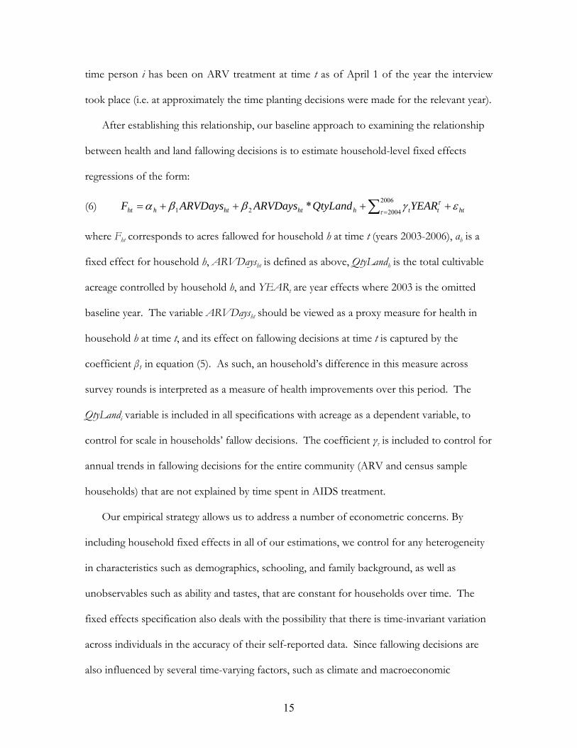
After establishing this relationship, our baseline approach to examining the relationship
between health and land fallowing decisions is to estimate household-level fixed effects
regressions of the form:
(6)
2006
200421 *
httthhththht YEARQtyLandARVDaysARVDaysF
where Fht corresponds to acres fallowed for household h at time t (years 2003-2006), αh is a
fixed effect for household h, ARVDaysht is defined as above, QtyLandh is the total cultivable
acreage controlled by household h, and YEARt are year effects where 2003 is the omitted
baseline year. The variable ARVDaysht should be viewed as a proxy measure for health in
household h at time t, and its effect on fallowing decisions at time t is captured by the
coefficient β1 in equation (5). As such, an household’s difference in this measure across
survey rounds is interpreted as a measure of health improvements over this period. The
QtyLandi variable is included in all specifications with acreage as a dependent variable, to
control for scale in households’ fallow decisions. The coefficient γτ is included to control for
annual trends in fallowing decisions for the entire community (ARV and census sample
households) that are not explained by time spent in AIDS treatment.
Our empirical strategy allows us to address a number of econometric concerns. By
including household fixed effects in all of our estimations, we control for any heterogeneity
in characteristics such as demographics, schooling, and family background, as well as
unobservables such as ability and tastes, that are constant for households over time. The
fixed effects specification also deals with the possibility that there is time-invariant variation
across individuals in the accuracy of their self-reported data. Since fallowing decisions are
also influenced by several time-varying factors, such as climate and macroeconomic

16
conditions, we include data from the census sample of adults to control for secular trends in
the survey area; the year effect dummy variables control for such effects. Thus, our key
identification assumption is that above and beyond the secular changes identified with data
from the census sample, ARV households do not differentially change their fallowing
decisions between survey rounds due to factors other than the receipt of treatment, which is
known to improve the health and extend the life of patients.
The empirical strategy described thus far will provide an estimate of the average effect of
health improvements on fallowing decisions, but we are particularly interested in
disentangling the productivity effect associated with a health shock from the discounting
effect. As such, we also estimate household fixed effect regressions of the following form:
(7) ht
nnhhtn
thhthtiht
DaysARV
YEARQtyLandDaysARVDaysARVF
)*(
)*(2006
200421
Variables are defined as in equation (6) and θnh represents household characteristic n for
household h. Household characteristics are chosen to characterize the labor endowment of
the household to help isolate the discount rate effect as described in Section II; these include
direct measures of household size as well as measures of household composition to describe
productive labor capacity. We make use of household-level controls, such as wealth and
various education measures, to isolate an independent effect of household size that is
consistent with our household labor endowment hypothesis.
All of the results we present use a balanced panel of adults who appear in both rounds of
the survey. Since some individuals exit the sample between round 1 and round 3 due to
death, relocation, or loss-to-follow up, selective attrition could give rise to biases in the
estimated treatment effects. In regressions not reported in the paper, we use our rich dataset
of observable characteristics to model the sample selection process in order to re-weight the

17
sample using the inverse probability weights (IPW) technique (Fitzgerald, Gottschalk and
Moffitt (1998) and Wooldridge (2002)). None of our main results reported below are
affected by these different estimation strategies.11
V. Results
Table 1 compares household characteristics of the census sample and the sample of HIV-
infected households receiving ARV therapy. Most household characteristics are not
significantly different between the two samples. On average, households in our sample have
a little more than 6 members and are headed by a 48-year-old with approximately 7 years of
formal education, and there is a significant amount of heterogeneity in these demographic
features. Differences between ARV and census households in acres of land owned are not
statistically significant either. Households in the census sample maintain planting decisions
over an average of 7.95 acres of land, compared to 6.77 acres for households in the ARV
sample. The average number of acres of land fallowed in round 1 are 4.8 and 3.71 in census
and ARV households, respectively. The difference in fallowed acres between the two
samples is nearly significant at the 10 percent level and seems to point toward slightly less
fallowing in ARV households. The only notable characteristic in which households differ
significantly is wealth, as proxied by radio ownership. The census sample households tend
to own slightly more than 1 radio per household, while the ARV sample tends to own
slightly less than 1 per household.
We begin our analysis by examining the relationship between ARV treatment and
health. Figure 1 plots the mean CD4 count in cells of twenty weeks before and after the
11 The IPW technique uses background and sexual behavior information from round 1 to predict the probability (pi) that an individual i will still be observed in a future round. This person receives a weight equal to 1/pi, thus individuals whose observable characteristics predict higher attrition rates have more weight in the regression analysis.

18
initiation of treatment for our study population.12 Figure 2 shows a similar relationship for
the body mass index (BMI) of patients. Both reveal a steady decline in health leading up to
treatment and dramatic improvements in the period afterwards. Table 2 reports results from
estimating equation 5 with CD4 count and BMI as the dependent variables. Here we see
that time on treatment has a significant impact on health (columns 1 and 3). We also find
that these health gains become smaller over time (columns 2 and 4), consistent with the
clinical observation that patients recover much of their health within the first 6-12 months
of treatment and typically maintain it thereafter.
Turning our attention to natural resource management decisions, we employ the
identification strategy described in equation 6 to estimate the average impact of health
improvements on the amount of land that a household leaves fallow. Table 3 presents our
results for two different outcome variables. Column 1 reveals the impact of treatment on
the percentage of land fallow, while Column 2 demonstrates the impact of treatment on total
acreage fallowed, controlling for the total amount of household land. Together they suggest
that the average effect of health improvements on fallow decisions is not statistically
different from zero13. The absence of a clear average treatment effect is consistent with our
ambiguous theoretical predictions and suggests the need for a more disaggregated approach
to disentangle the competing effects of health on labor productivity and discount rates.
Our first approach to separately identify these effects uses several measures of a
household’s labor endowment to estimate equation 7. We focus on labor endowments with
the supposition that larger households may be better equipped to reallocate labor to
12 Due to the low frequency at which CD4 count is measured, we chose a group size that is large enough to produce a relatively smooth curve. When mean CD4 counts are calculated for intervals of less than 10 weeks, the figure looks similar. Likewise, a similar pattern is evident when mean CD4 count is calculated in each time interval. 13 Since ARV households have 6.77 acres on average, the effect of ARV treatment on fallowing, as one would expect, is nearly identical in the two specifications.

19
agricultural activities, thus minimizing the importance of the productivity effect on overall
acreage fallowed and potentially allowing us to identify the competing discount rate effect.
Table 4 presents results using specifications with various combinations of household size,
household size squared, and the age structure of the household. Since the productivity effect
is likely to be least pronounced in the largest of households, we also include a dummy
variable indicating whether a household has more than seven members living at home, which
corresponds to a household size at approximately the 75th percentile.
The first column of Table 4 shows that the effect of health improvements on fallowed
acres are decreasing in family size, but increasing in the square of family size. When we turn
our attention to families at or above the 75th percentile in terms of family size, we see that
health improvements lead to substantial increases in acreage fallowed – 100 days on
treatment leads to roughly one-third of an acre of additional fallow.14 Column 4 shows that
households with, on average, younger family members increase their fallowed acres more as
they get healthier, relative to households with older members. Since younger families are
likely to have more productive labor available, this is further evidence of labor substitution in
the face of a health shock and suggests that younger families are less likely to have fallowed
acres impacted by a productivity effect. Household size remains a significant predictor of
the impact of treatment, but with a smaller coefficient, when the number of children under
the age of six is included in the regression (column 5). Taken together, these results provide
strong support for our contention that a large labor endowment minimizes the productivity
impacts from a health shock, leaving the discount rate effect to dominate, and thus leading
to greater levels of environmental conservation in response to health improvements.
14 When both measures of household size are included, household size larger-than-seven remains significant at the 10% level, while the other size coefficients are insignificant (column 3).

20
Of course, our measures of labor endowments may be capturing the influence of other
household characteristics that might be correlated with household size. Since non-
agricultural asset wealth can be liquidated to help cope with health shocks, and household
size and wealth may be correlated, we confirm that the effect of household size is robust to
the inclusion of controls for asset wealth. Table 5 presents results when we include a
measure of household wealth and an indicator variable for whether the household head
completed secondary school. Column 1 suggests that wealthier families conserve more as
they become healthier relative to poorer families, and column 2 suggests that this effect is
independent of the effect of family size. Column 3 indicates a similarly positive influence of
education, but the results shown in Column 4 indicate that the education coefficient is
actually capturing a collinear effect of family size. Here again we see that the effect of
household size persists, and the same is true in column 5 where controls for both education
and wealth are included. The significant coefficients on land holdings, family size, and age
are stable through all specifications providing evidence that the household labor endowment
influences resource management decisions in a manner consistent with our theory.
Finally, we re-run our preferred specifications using only 2003 and 2006 data to confirm
that the longer recall periods associated with the fallow data from 2004 and 2005 were not
biasing our results. As revealed in Table 6, our results are robust to this alternative
approach. Land holdings, household size, and age all remain significant and of similar
magnitude. Non-agricultural wealth is only significant at the 10% level in one specification
(see column 3), but this appears to be driven by the increase in standard errors associated
with our smaller panel while our point estimates remain stable.
VI. Conclusion

21
In this paper, we developed a simple model of natural resource management within
subsistence households that face health shocks. The impact of health operates through two
distinct and competing channels by influencing labor productivity and planning horizons.
Sicker households are less able to extract natural resources, but also have a diminished
incentive to conserve them. Thus, the net impact of health shocks is ambiguous. Which
effect dominates is shown to depend, in part, on household size since larger households,
which are better equipped to reallocate labor in response to the illness of a family member,
are less susceptible to the influence of health on household productivity.
We then examine this problem empirically by examining the relationship between health
improvements associated with AIDS treatment and household land fallowing decisions.
The average effect of treatment on land fallowing is zero. An examination based on
household characteristics, however, reveals more heterogeneous impacts. In particular, large
households fallow more land as they become healthier and these impacts are robust to a
wide range of specifications. These results are consistent with model predictions and
together provide strong evidence for both productivity and discount rate effects in response
to health changes.
These findings have important policy implications. The UN Millennium Development
Goals include health, wealth, and environmental targets, which some have argued may be in
conflict with one another. Health improvements in small households will greatly improve
household consumption, but perhaps at the expense of the environment. In contrast, large
households may conserve more in response to health improvements, but consumption
impacts may be small. As such, a differentiated approach may be required to ensure that all
goals are met in the most efficient manner possible.

22
VII. References Ashenfelter, Orley and James Heckman. 1974. “The Estimation of Income and Substitution Effects in a Model of Family Labor Supply.” Econometrica 42:73-86. Becker, Gary. 1965. “A Theory of the Allocation of Time.” Economic Journal 75:493-517. Bünemann, E.K., P.C. Smithson, B. Jama, E. Frossard and A. Oberson. 2004. “Maize productivity and nutrient dynamics in maize-fallow rotations in western Kenya.” Plant and Soil. 264: 195-208. Central Bureau of Statistics. 1999. Kenya 1999 Population and Housing Census. Central Bureau of Statistics: Nairobi. Chequer, P. et al. 1992. “Determinants of Survival in Adult Brazilian AIDS Patients, 1982-1989.” AIDS 6:483-487. Coetzee, David et al. 2004. “Outcomes After Two Years of Providing Antiretroviral Treatment in Khayelitsha, South Africa.” AIDS 18:887-895. Cohen, Jonathan et al. 2004. “Addressing the Educational Void During the Antiretroviral Therapy Rollout,” AIDS 18:2105-2106. Deolalikar, A.1988. “Nutrition and Labor Productivity in Agriculture: Estimates for Rural South India.” Review of Economics and Statistics 70: 406-13 Fitzgerald, John, Peter Gottschalk, and Robert Moffitt. 1998. “An Analysis of the Impact of Sample Attrition on the Second Generation of Respondents in the Michigan Panel Study of Income Dynamics.” Journal of Human Resources 33(2):251-99. Goldie et al., 2006 Haggblade, S., G. Tembo, and C. Donovan. 2003. Household Level Financial Incentives to Adoption of Conservation Agricultural Technologies in Africa. Working Paper 9. Lusaka, Zambia: Food Security Research Project. Jacoby, Hanan G. and Emmanuel Skoufias. 1997. “Risk, Financial Markets, and Human Capital in a Developing Country.” Review of Economic Studies 64:311-335. Kochar, Anjini. 1995. “Explaining Household Vulnerability to Idiosyncratic Income Shocks.” The American Economic Review Papers and Proceedings 85:159-164. Koenig, Serena P., Fernet Leandre, and Paul E. Farmer. 2004. “Scaling-up HIV Treatment Programmes in Resource-Limited Settings: The Rural Haiti Experience.” AIDS 18:S21-S25.

23
Laurent, Christian et al. 2002. “The Senegalese Government’s Highly Active Antriretroviral Therapy Initiative: An 18-month Follow-up Study.” AIDS 16:1363-1370. Loevinsohn, M., and S. Gillespie. 2003 “HIV/AIDS, Food Security and Rural Livelihoods: Understanding and Responding.” IFPRI Renewal Working Paper 2. Mamlin, Joe, Sylvester Kimaiyo, Winstone Nyandiko, and William Tierney. 2004. Academic Institutions Linking Access to Treatment and Prevention: Case Study. World Health Organization: Geneva. Marins, Jose Ricardo P. et al. 2003. “Dramatic Improvement in Survival Among Adult Brazilian AIDS patients.” AIDS 17:1675-1682. Morgan, Dilys et al. 2002. “HIV-1 Infection in Rural Africa: Is There a Difference in Median Time to AIDS and Survival Compared with That in Industrialized Countries?” AIDS 16:597-603. Mosier, A.R. 1998. “Soil processes and global change.” Biology and Fertility of Soils. 27:221–229. Paxson, Christina. 1992. “ Using Weather Variability to Estimate the Response of Savings to Transitory Income in Thailand.” American Economic Review 82: 15-33. Pitt, M., Rosenzweig, M.and N Hassan. 1990. “Productivity, Health, and Inequality in the Intrahousehold Distribution of Food in Low-Income Countries.” American Economic Review 80:1139-56. Piwoz, E., and E. Preble. 2000. “HIV/AIDS and Nutrition: A Review of the Literature and Recommendations for Nutritional Care and Support in sub-Saharan Africa.” Discussion Paper SARA Project, USAID, Washington DC. Sanchez, Pedro A. 2002. “Soil fertility and hunger in Africa.” Science. 295(5562):2019-2020. Sanchez, Pedro A. 1999. “Improved fallows come of age in the tropics.” Agroforestry Systems. 47: 3–12. Semba, R. D., and A. M. Tang. 1999. “Micronutrients and the Pathogenesis of Human Immunodeficiency Virus Infection.” British Journal of Nutrition, 81(3), 181–189. Strauss, John and Duncan Thomas. 1995. “Human Resource: Empirical Modeling of Household and Family Decisions,” in Jere Behrman and T.N. Srinivasan, eds. Handbook of Development Economics Vol. 3, Part 1. Swinkels, R.A., S. Franzel, K.D. Shepherd, E. Ohlsson and J.K. Ndufa. 1997. “The economics of short rotation improved fallows: Evidence from areas of high population density in western Kenya.” Agricultural Systems. 55: 99–121.

24
Szott L.T., C.A. Palm and R.J. Buresh. 1999. “Ecosystem fertility and fallow function in the humid and subhumid tropics.” Agroforestry Systems. 47:163–196. Thirumurthy, Harsha, Markus Goldstein, and Joshua Graff Zivin,. 2008. “The Economic Impact of AIDS Treatment: Labor Supply in Western Kenya.” Journal of Human Resources 43(3):511-552. UNAIDS. 2010. AIDS Epidemic Update, 2009. Geneva: Joint United Nations Programme on the HIV/AIDS. Wooldridge, Jeffrey. 2002. “Inverse Probability Weighted M-estimators for Sample Selection, Attrition, and Stratification.” Portuguese Economic Journal 1(2):117-39. Wools-Kaloustian, Kara, et al. 2006. “Viability and Effectiveness of Large-scale HIV Treatment Initiatives in Sub-Saharan Africa: Experience from Western Kenya.” AIDS 20:41-48. World Health Organization. 2003. Nutrient Requirements of People Living with HIV/AIDS: Report of a Technical Consultation. World Health Organization: Geneva.

25
Table 1: Summary Statistics and Comparisons across Samples Census Sample ARV Sample P-value*
Mean Std. Dev. Mean Std. Dev. Number of households 489 140 Demographics Household size 6.04 2.34 6.17 2.78 0.60
Average age of household members 24.62 11.65 24.06 9.34 0.56
Age of household head 48.05 15.38 47.28 12.84 0.55
Number of family members > 7 0.29 0.45 0.27 0.45 0.66
Wealth
Radios owned by household 1.05 0.78 0.86 0.80 0.01
Education of Household Head
Years of schooling 6.86 3.98 7.04 3.97 0.63
Completed primary school 0.43 0.50 0.44 0.50 0.92
Completed secondary school 0.22 0.42 0.25 0.43 0.48
Land Holdings
Total quantity of land (acres) 7.93 10.65 6.61 9.92 0.17
Acres of land fallowed (Round 1) 4.63 8.11 3.69 6.89 0.18 *P-values provided for two-tailed t-tests; equal variances between the two samples are not assumed.

26
Table 2: Impact of ARV Treatment on Health, with Individual Fixed Effects
CD4 BMI (1) (2) (3) (4) # days after start of ARVs 0.3170 0.5119 0.003133 0.007861 (7.24)*** (4.92)*** (11.39)*** (11.99)*** days after squared -0.0003 -0.000006 (2.06)** (7.87)*** Observations 117 117 672 672 Number of individuals 45 45 37 37 R-squared 0.42 0.46 0.17 0.24
Absolute value of t statistics in parentheses. Regressions include individual (patient) fixed effects. * significant at 10%; ** significant at 5%; *** significant at 1%

27
Table 3: Impact of ARV Therapy on Fallow Land (% and Acres of Land)
(1) (2) Dependent Variable: Percent Fallow Acres Fallow Days on ARV 0.00002 -0.00113 (0.00004) (0.00060)* Days on ARV * Qty. of Land 0.00019 (0.00005)*** HH Fixed Effects Yes Yes Year Effects Yes Yes Number of Households 629 629
Standard errors in parentheses. Regressions include household fixed effects. * significant at 10%; ** significant at 5%; *** significant at 1%

28
Table 4: Impact of ARV Therapy on Fallow Land (Acres): Labor Endowment Effects
Standard errors in parentheses. Regressions include household fixed effects. * significant at 10%; ** significant at 5%; *** significant at 1%
(1) (2) (3) (4) (5) Dependent Variable: Acres Fallow Days on ARV 0.0004 -0.0019 0.0005 0.0014 -0.0026 (0.0016) (0.0006)*** (0.0016) (0.0012) (0.0008)*** Days on ARV * Qty. of Land 0.0002 0.0002 0.0002 0.0002 0.0002 (0.0000)*** (0.0000)*** (0.0000)*** (0.0000)*** (0.0000)*** Days on ARV * HH Size -0.0012 -0.0009 (0.0006)** (0.0006) Days on ARV * (HH Size)2 0.0001 0.0001 (0.0000)*** (0.0001) Days on ARV * HH Size > 7 0.0032 0.0034 0.0032 0.0027 (0.0010)*** (0.0018)* (0.0010)*** (0.0010)*** Days on ARV * Avg. Age -0.0001 (0.0000)*** Days on ARV * # Children ≤5 0.0014 (0.0009) HH Fixed Effects Yes Yes Yes Yes Yes Year Effects Yes Yes Yes Yes Yes Observations 2218 2218 2218 2218 2218 Number of hhn 629 629 629 629 629

29
Table 5: Impact of ARV Therapy on Fallow Land (Acres): Robustness to Inclusion of Other Characteristics (1) (2) (3) (4) (5) Dependent Variable: Acres Fallow Days on ARV -0.0028 -0.0001 -0.0017 0.0006 -0.0005 (0.0008)*** (0.0014) (0.0007)*** (0.0013) (0.0014) Days on ARV * Qty. of Land 0.0001 0.0002 0.0002 0.0002 0.0002 (0.0000)*** (0.0000)*** (0.0000)*** (0.0000)*** (0.0000)*** Days on ARV * Wealth 0.0021 0.0015 0.0013 (0.0006)*** (0.0007)** (0.0007)** Days on ARV * HH Size>7 0.0027 0.0032 0.0028 (0.0010)*** (0.0010)*** (0.0010)*** Days on ARV * Avg. Age -0.0001 -0.0001 -0.0001 (0.0000)*** (0.0000)*** (0.0000)** Days on ARV * Education 0.0022 0.0016 0.0013 (0.0010)** (0.0010) (0.0010) HH Fixed Effects Yes Yes Yes Yes Yes Year Effects Yes Yes Yes Yes Yes Observations 2207 2207 2204 2204 2196 Number of hhn 626 626 625 625 623 Standard errors in parentheses. Regressions include household fixed effects. * significant at 10%; ** significant at 5%; *** significant at 1%

30
Table 6: Impact of ARV Therapy on Fallow Land (Acres): 2003 and 2006 data only
(1) (2) (3) (4) Dependent Variable: Acres Fallow Days on ARV -0.00153 0.0018 0.0004 0.0001 (0.00103) (0.0021) (0.0024) (0.0024) Days on ARV * Total Land 0.00025 0.0003 0.0002 0.0002 (0.00008)*** (0.0001)*** (0.0001)*** (0.0001)*** Days on ARV * HH Size >7 0.0038 0.0033 (0.0016)** (0.0016)** Days on ARV * Avg. Age -0.0002 -0.0002 -0.0002 (0.0001)** (0.0001)** (0.0001)** Days on ARV * Wealth 0.0021 0.0016 (0.0011)* (0.0011) HH Fixed Effects Yes Yes Yes Yes Year Effects Yes Yes Yes Yes Observations 1109 1109 1104 1104 Number of Households 627 627 624 624 R-squared 0.03 0.05 0.05 0.05
Standard errors in parentheses. Regressions include household fixed effects. * significant at 10%; ** significant at 5%; *** significant at 1%

31
Figure 1: CD4 Count Before and After Initiation of ARV Therapy
100
150
200
250
300
Mea
n C
D4
co
unt
-40 -20 0 20 40 60 80Weeks Before/After ARV Initiation
Figure 2: Body Mass Index Before and After Initiation of ARV Therapy
18
20
22
24
26
Mea
n B
MI
-40 -20 0 20 40 60 80Weeks Before/After ARV Initiation