HEAT AND MASS CONVECTION - UPM

Heat and mass convection. Boundary layer flow page 1

HEAT AND MASS CONVECTION. BOUNDARY LAYER FLOW

Heat and mass convection ............................................................................................................................. 1

Heat convection: what it is ........................................................................................................................ 1 Types of heat convection .......................................................................................................................... 2 A brief on Fluid Mechanics ...................................................................................................................... 3

Continuity equation ............................................................................................................................... 4 Momentum equation ............................................................................................................................. 5 Energy equation .................................................................................................................................... 5 Mass transport equation ........................................................................................................................ 5 Constitutive equations ........................................................................................................................... 6

Introduction to non-dimensional parameters ............................................................................................ 7 Boundary layer flow................................................................................................................................ 10

Non-slip condition............................................................................................................................... 10 Boundary layer forced-flow over a flat plate ...................................................................................... 10 Thermal boundary layer and solutal boundary layer in a forced-flow over a flat plate ...................... 15

Reynolds analogy between momentum and energy equations ............................................................... 18 Steps to solve heat and mass convection problems ............................................................................. 20

Temperature and pressure effects on fluid properties ............................................................................. 21 Forced and natural convection (aside) .................................................................................................... 23 Convection with phase change (aside) .................................................................................................... 23 Heat exchangers (aside) .......................................................................................................................... 23

HEAT AND MASS CONVECTION

We present here some basic modelling of convective process in Heat and mass transfer. Heat diffusion, mass diffusion, and heat radiation are presented separately. Furthermore, mass convection is only treated here as a spin-off of the heat convection analysis that takes the central focus.

Heat convection: what it is

There cannot be any convected heat, since heat is only defined as thermal-energy flow through an impermeable surface due to a temperature difference across. What we call heat convection is the effect of a fluid flow on heat conduction at a fluid-washed wall; i.e. we intend to apply Newton's law of cooling instead of Fourier's law (see Physical transport phenomena in Heat and mass transfer): What is heat (flux) convection? ( ) nq h T T k T∞≡ − = − ∇ (1) (where ∇n stands for the normal gradient at the wall), aiming at substituting the effect of a real flow field by an empirical boundary condition at the wall, i.e. with the convective coefficient h in (1) found from global measurements of temperatures and heat fluxes in experiments, instead of by analytically solving the fluid flow (Navier-Stokes' equations) and using (1) to deduce h. Internal thermal energy (not heat) is convected with the fluid flow, in an amount dependent on a reference energy-level (reference temperature), usually referred to the ambient or sink temperature. When the increase in internal thermal

http://webserver.dmt.upm.es/%7Eisidoro/bk3/c11/Heat%20and%20mass%20transfer.pdf

http://webserver.dmt.upm.es/%7Eisidoro/bk3/c11/Heat%20conduction.pdf

http://webserver.dmt.upm.es/%7Eisidoro/bk3/c11/Mass%20Transfer.pdf

http://webserver.dmt.upm.es/%7Eisidoro/bk3/c11/Heat%20and%20mass%20transfer.pdf


energy is due to heat transfer at a source, the energy balance for a fluid flow at constant pressure without phase changes and reactions is Q mc T= ∆

, what shows that, the same thermal load can be transported by a high mass-flow-rate flow with small temperature jump, or by a low mass-flow-rate flow with high temperature jump, and that thermal-carrier fluids should have high thermal capacity. Notice that in Fluid Mechanics, there is no Newton's law of cooling, and the only heat-transfer term to be included is Fourier's conduction (and in very special cases thermal radiation emission or absorption through the media).

Types of heat convection

Heat convection problems may be classified according to: • Time variation, as steady or unsteady convection. Only a marginal fraction of applications require

transient convection analysis (e.g. when the onset of natural convection in a fluid layer heated from below, is studied).

• Flow origin, as forced convection or natural convection. Forced convection occurs when the fluid flow is imposed by other agent than the heat-transfer phenomena under study, i.e. by a pump, a fan, or natural convection from other objects. Natural or free convection occurs when the fluid flow appears as a consequence of the heat-transfer phenomena under study, due to buoyancy forces caused by density gradients in an external force field. Natural convection takes place in all heat convection problems under gravity, but when forced convection is imposed, the latter usually overcomes the former (a combination of the two must be considered at small forcing speeds). Forced convection greatly enhances heat transfer, but demands power consumption. (According to this division, the internal flow in a heat-pipe, due to capillary pumping, is forced, in spite of not consuming external power. Thermo-capillary convection, like Marangoni convection, is also not considered in these notes.)

• Flow regime, as laminar flow or turbulent flow. Turbulent flow is the rule in engineering applications, but laminar flow always exists in some regions, like close to walls and entrance regions. Turbulent convection greatly enhances heat transfer, but increases power consumption too.

• Flow topology, as internal flow or external flow. Internal flow is when we focus on the fluid flowing inside pipes and ducts, whereas external flow is when we focus on the fluid flowing outside pipes and ducts, or around any other solid object. The distinction is not so clear when one considers a portion of a duct (e.g. a flat plate), or open-channel flow, although all these cases are traditionally considered external flow. Some other times, flow topology depends on the detail of the analysis, as in shell-and-tube heat exchanger, when heat transfer can be considered external convection of the shell-fluid around the tubes, or internal convection of a shell-ducted flow to the walls (mainly the internal walls), as for compact plates heat exchangers.

• Flow phases, as single-phase or multi-phase flows. An intermediate type is stratified flow (i.e., homogeneous, heterogeneous: stratified, two bulk phases, and disperse). This division is not only important for permanent multi-phase flow, but for vaporising and condensing flows.


• Flow detail, as detailed heat convection or global heat convection. Most of the times, the empirical approach to convection heat transfer only looks for global values of the convective coefficient around a solid, or along a pipe; but there are cases where temperature variations along the wall must be resolved, either during experiments to compute global h-values by integration, or during analysis to know if some temperature limit is locally exceeded, and for this purpose a local approach is of interest.

• Flow compressibility is seldom important in heat convection. Flow reactivity, if any, is considered aside as a distributed energy source or sink. Other important fluid flow divisions, like viscous and inviscid flows, or 1D- 2D- and 3D- flows, are of little importance in the study of heat transfer by convection, because of the global empirical approach followed.

• Thermal boundary regulation. Two basic cases are considered: constant wall temperature, and constant heat flux, the former being more closely approached in practice (it is simpler to regulate the temperature of the wall than the heat flux through it, and there temperature is maintained in phase changes of a pure substance), but the latter being simplest to model, since it means a constant source term in the energy balance (and it is the actual case in counter-flow heat exchangers with similar fluid flows). As a matter of fact, both types of control can be advantageously used, as in hot-wire velocimetry (or hot-wire anemometry), where either the wire temperature is controlled (regulating its electrical resistance R(T) and measuring the required power as a function of flow speed, Q ), or the supplied power to the wire is fixed, and the steady-state temperature difference between wire and fluid measured. The steady-state energy balance,

2w( )Q V R KA T T∞= = − , allows a calibration against relative flow speed, v, when a cooling law is

assumed (e.g. K a b v= + ). Air is the most ubiquitous fluid in heat convection. All terrestrial animals and most equipment transfer heat to the environment by natural convection in air, with a typical convection coefficient value in the range h=5..10 W/(m2·K). For simple cooling/heating load calculations with wind effects, Duffie and Beckmann (1991) rule h=a+bvwind, with a=3 W/(m2·K) and b=3 J/(m3·K) may be a first approximation. Notice that the convective coefficient depends on fluid type, flow type, and geometry. For instance, for natural convection from a plate in air, correlations for h in (1) are (see details in Forced and natural convection) h=a(T−T∞)1/4, with a=2.4 W/(m2·K5/4) for the upper face of a horizontal surface, a=1.3 W/(m2·K5/4) for the lower face of a horizontal surface (stable vertical gradient), and a=1.8 W/(m2·K5/4) for a vertical surface.

A brief on Fluid Mechanics

Fluid Physics encompasses the nature of fluids (their structure and properties), the fluid forces within and on the boundaries, the transport of mass, momentum and energy, and possible effects of reactive processes, electromagnetic interactions, and so on; Fluid Mechanics concentrates on fluid forces and the transport of momentum. Our interest here is on the transport of energy, but this is linked to the transport of momentum and cannot be studied apart when fluid flow exists; that is why we are presenting below an ad hoc summary of the general equations, a rather complicated formulation with the three simple objectives:

http://webserver.dmt.upm.es/%7Eisidoro/bk3/c12/Forced%20and%20natural%20convection.pdf



• To have an overview of the full equations which are pre-programmed in computational-fluid-dynamic codes (as commercial CFD packages). The user is in charge of selecting the appropriate terms in the equations, and setting the initial and boundary conditions, but the equations are automatically solved.

• To have an idea of the terms retained and the terms neglected in some simple heat-and-mass transfer problems to be analysed in detail, as the boundary-layer flow, and the pipe flow.

• To better understand the rational for the grouping of dimensional variables into the traditional non-dimensional parameters.

The description of fluid flow makes use of the continuum model, and on the concept of fluid particle, an infinitesimal control system in local thermodynamic equilibrium. Once a reference frame is selected, the motion of fluid particles may be described in two ways: • Eulerian description, where the unit volume is fixed to the spatial reference frame, and the motion of

the particle that at every instant happens to pass by this position, is specified. • Lagrangian description, where the unit volume moves with the flow relative to the spatial reference

frame, and the motion of the same particle at each position, is specified. Passing from the most-intuitive Lagrangian to the most-used Eulerian description is based on Reynolds transport theorem:

( ) CV

CV

CM CV 0 CV 0 CV CV

( )CM

( ) ( ) ( )

V f tA

V t V t t A t t V A

d d dV dV v v ndA dV v ndAdt dt t tΦ ∂φ ∂φφ φ φ

∂ ∂≠

= =

= = + − ⋅ → + ⋅∫ ∫ ∫ ∫ ∫ (2)

which says that, for of any conservative property (Φ may be mass, momentum, or energy) in a control mass CM (its value being the integral of the specific function over the volume; e.g. φ would be mass per unit volume, ρ), the variation with time in a permeable system can be computed as the integral of the specific function within the control volume CV, plus the flux of that variable over the permeable area. Passing from area integrals to volume integral is based on Gauss-Ostrogradski’s divergence theorem:

( )CV CV

CV CV CV

CM 0V A

vdV v ndA

V A V

d dV v ndA v dVdt t tΦ ∂φ ∂φφ φ

∂ ∂

∇⋅ = ⋅∫∫∫ ∫∫ = + ⋅ = + ∇ ⋅ = ∫ ∫ ∫

(3)

which is applied to an infinitesimal volume to get the general equations of Fluid Mechanics: continuity equation, momentum equation, and energy equation.

Continuity equation The continuity equation is the mass balance (dmCM/dt=0) for a dV system; with φ=ρ we get from (3):

( ) 0vt

∂ρ ρ∂

+ ∇ ⋅ = , or D 0

Dv

tρ ρ+ ∇ ⋅ =

(4)


where the convective derivative D() / D () / ()t t v∂ ∂≡ + ⋅∇ is often introduced to make the writing more

compact. In most heat and mass transfer problems, the continuity equation can be reduced to 0v∇ ⋅ =

because density changes are usually negligible.

Momentum equation The momentum equation is the linear-momentum balance ( ( )CM

/ V Ad mv dt F F F= = +

), applied to a dV system; with vφ ρ=

we get from (3), using the convective derivative:

( ) ( ) ( )D '

Dvv vv g p gz

t t∂ ρ

ρ ρ τ ρ ρ τ∂

= + ∇ ⋅ = ∇ ⋅ + = −∇ + + ∇ ⋅

(5)

where τ is the stress tensor (such that the force per unit area of normal vector n is f nτ= ⋅

), g is any volumetric force field (e.g. gravity), p is fluid pressure (one third of the trace of the stress tensor), and 'τ the viscous component of the stress tensor. In most heat and mass transfer problems (5) can be reduced to the so-called Boussinesq approximation (constant-density flow except for the buoyancy term, proportional to the thermal-expansion coefficient α, named in honour of the French Academician V. J. Boussinesq, who studied in the late 19th c. convective cooling and turbulence):

( ) 20

D 1D z

v p g T T i vt

α νρ

∇= − − − − + ∇

(5a)

where ν≡µ/ρ is the kinematic viscosity and µ the dynamic viscosity.

Energy equation The energy equation is the energy balance ( ( )CM

/d me dt Q W= + ) for a dV system; with φ=ρe we get from (3):

( )DD

e q vt

ρ τ= −∇ ⋅ + ∇ ⋅ ⋅

(6)

which in most heat and mass transfer problems is expressed in terms of temperature:

D / ' :Dp

Tc q TDp Dt vt

ρ α τ= −∇ ⋅ + + ∇

(6a)

Most of the times energy terms other than the accumulation ρcpDT/Dt and the heat flux q−∇ ⋅

terms, are grouped under a dissipation variable φ (energy release per unit volume), as seen in Heat and Mass Transfer.

Mass transport equation The (global) mass-transport equation is the continuity equation above; what we deal with here is the species-balance equation in a mixture, (dmi,CM/dt=Wi, for any species i, with Wi being a possible i-species production term by chemical reactions), for a dV system. Now, besides substituting φ=ρι≡mi/V in (3), one has to use in (3) the i-species own velocity, iv , related to the mass-averaged velocity v by the conservation equation i iv vρ ρ=∑ , and the definition of diffusion velocity di iv v v≡ −

, what yields:


( ) ( ) ( ) ( )di i i

i i i i i i iv w v v v jt t t

∂ρ ∂ρ ∂ρρ ρ ρ ρ∂ ∂ ∂

+ ∇ ⋅ = = + ∇ ⋅ + ∇ ⋅ = + ∇ ⋅ + ∇ ⋅

(7)

where di i ij vρ≡

is the flux density of species i through a (global) fluid particle. With the convective derivative:

DD

ii i iv w j

tρ ρ+ ∇ ⋅ = − ∇ ⋅

(7a)

wi being a possible i-species production term per unit volume.

Constitutive equations To solve a Fluid Mechanics problem, i.e. to find the velocity field, pressure field and temperature field ( ), ,v p T in terms of position and time ( ),x t , besides the initial and boundary conditions of the particular problem at hand, the above balance equations of mass, momentum, and energy, must be supplemented with some general constitutive equations that relate the additional variables ( ), , , , , ,i ie q j wρ τ φ

to the main variables ( ), ,v p T , i.e. the equation of state at equilibrium, ρ=ρ(T,p) and e=e(T,p), and the main one in Fluid Mechanics, a relation between fluid strain-rate and stress, first proposed by Newton in 1687 as,

/v yτ µ= − ∂ ∂ , and in a more general way named Navier-Poisson's law:

( ) ( ) ( )2 2' 2 ( )3 3

TV VpI pI v I pI v v v Iτ τ µε µ µ µ µ µ = − + = − + + − ∇ ⋅ = − + ∇ + ∇ + − ∇ ⋅

(8)

which enters into the momentum balance as:

( )( ) ( )0

2 22'3Vp p v v v p v

ρ

τ τ µ µ µ τ µ∇ = ∇ ⋅ = −∇ + ∇ ⋅ = −∇ + ∇ + ∇ ∇ ⋅ + − ∇ ∇ ⋅ = ∇ ⋅ = −∇ + ∇

(8a)

Besides state equations and the strain-rate to stress relation, one needs a heat-rate relation (our well-known Fourier's law, q k T= − ∇

, or its extension to multi-component-diffusing systems,

di i iq k T v hρ= − ∇ + ∑

, with the enthalpy of species i, hi, being deduced from the state equations adopted), plus appropriate dissipation laws for φ, plus the mass diffusion rate equations, namely the extended Fick's law and Arrhenius's law: ( )/i i i Sj D c Tρ ρ= − ∇ +

(9)

w MM

B ERTi i i i

i

ia

ai

= −FHG

IKJ

−FHG

IKJ∏( ) exp" '

'

ν ν ρν

(10)

where Di is the coefficient of mass diffusion of species i in a given mixture due to concentration gradients, cS is the Soret coefficient of mass diffusion due to thermal gradients (usually negligible), wi is the mass of species i produced (by unit time and volume of mixture) due to chemical reactions, νi'' and νi' the stoichiometric coefficients for the forward and backward reaction considered (one wi must be considered for each reactions), and Ba and Ea two empirical Arrhenius coefficients. The kinetic theory of gases provides a simple (although sometimes not very accurate) formulation of all the transport


coefficients and equations of state in terms of pressure, temperature and composition, but in practice one usually resorts to tabulated experimental data. As no reaction is to be considered here, and Soret effects are neglected, the only term entering into the mass-diffusion balance is: 2

i i ij D ρ∇ ⋅ = − ∇

(11) In summary, substituting these constitutive relations in the balance equations, the partial differential equations that solve a heat and mass transfer problem, with fluid flow but nearly constant density, are:

Mass balance (continuity): 0v∇ ⋅ = (12)

Species balance: 2DD

i ii i

y wD yt ρ

= ∇ + (13)

Momentum balance: ( ) 20

D 1D z

v p g T T i vt

α νρ

∇= − − − − + ∇

(14)

Energy balance: 2DD p

T a Tt c

φρ

= ∇ + (15) where /i iy ρ ρ≡ is the mass fraction of species i in the mixture. Notice that the i-species diffusivity in the mixture, Di, the momentum diffusivity (kinematic viscosity) ν, and thermal diffusivity, a=k/(ρcp), all have dimensions of square length divided by time. Finally recall the definition of the convective derivative. D() / D () / ()t t v∂ ∂≡ + ⋅∇

, which reduces to D() / D ()t v= ⋅∇ in the steady-state case.

Introduction to non-dimensional parameters

In all fields of physical sciences, but particularly in Fluid Mechanics, and above all in Heat and Mass Transfer, there is such a number of parameters interplaying in each problem, that it is most convenient for us to group them if possible, and there is a general principle applicable for that, namely, the Pi-Buckingham Theorem (ASME, 1915), which states that a physical equation with N variables whose magnitudes can be expressed in terms of M independent physical units, is equivalent to a non-dimensional physical equation with N−M non-dimensional variables. Before attempting that grouping, however, some remarks are appropriate. Firstly, the number of independent physical units, M, is not a universal invariant but a universal agreement, and the metre-unit (m) could be totally skipped if lengths were measured with the second-unit (s) and the universal law for the speed of light in vacuum c=1 assumed, instead of giving dimensions to this universal invariant, c=3·108 m/s. Secondly, and most important, if working with non-dimensional variables is so advantageous, why most physical subjects are learnt using dimensional magnitudes? The answer is that we, humans, want to compare every magnitude with our own measurements: lengths with the length of our arm span, masses with the mass of a stone we can throw, times with our heart period, and so on, and each of our anthropocentric units we introduce, contributes to one of the M-basic magnitudes mentioned above (seven in the SI: m, kg, s, K, A, cd, and mol).


For the grouping of dimensional variables to get non-dimensional parameters, one may follow an ad hoc approach. For instance, in thermal convection studies, one may reason that the convective coefficient h must be a function of the fluid properties (k,ρ,cp,µ), and the characteristic fluid-velocity gradient v/L, i.e. h=h(k,ρ,cp,µ,v/L), and say that the combinations /Nu hL k≡ , /Re vLρ µ≡ , and /pPr c kµ≡ , are 'the usual choice', or 'the standard rule', but someone might ask why not another combination, and if there is a rational behind. Adding that the rational is to compare heat convected (h∆T) against heat conducted if the fluid was quiescent (k∆T/L), to compare change of momentum ((ρv)v) against viscous stress (µ(v/L)), and to compare momentum diffusivity (ν≡µ/ρ) against thermal diffusivity (a=k/(ρcp)), may seem enough justification already. But the most conclusive explanation of why those parameters and their meaning, comes from an order-of-magnitude analysis of the general equations presented above, both the balance equations and the boundary conditions, namely: Thermal boundary condition at a wall. From the definition of heat convection coefficient:

( ) nT hLq h T T k T h T k NuL k∞

∆≡ − = − ∇ → ∆ ≈ → ≡ (16)

what teaches that a non-dimensional parameter, Nu, can be defined to measure the ratio of heat flux transferred with convection to that without convection; it is named Nusselt number in honour of the great thermal engineer Wilhelm Nusselt, who introduced it in his 1915 pioneering article "The Basic Laws of Heat"; the 'number' ending is the traditional designation of non-dimensional parameters (no physical units, just the number). In spite of heat convection being always greater than a corresponding heat conduction, Nu may be smaller than unity if one choose for it a length smaller than the boundary-layer thickness (e.g. when using the diameter for fine wires). Mass balance. From the continuity equation:

0 0yx

x y

vvvL L

∇ ⋅ = → + = (17)

what teaches that, if there is a change of fluid speed along one direction (vx/Lx), it must be a balancing change of fluid speed along another direction (the flow must be at least two-dimensional); i.e., in a one-dimensional flow (in Cartesian coordinates), the speed cannot change along a streamline (∂v/∂x=0). Notice that the fact that the two velocity-gradients be of equal magnitude does not mean that the longitudinal flow must be of the same order as the transversal flow, the paradigmatic case being the boundary-layer flow to be analysed below, where the longitudinal flow vx is dominant, i.e. vy<<vx, but still ∂vy/∂y=−∂vx/∂x. Momentum balance. From the longitudinal momentum equation, assuming gravity effects irrelevant, and expanding the convective derivative:


2 2 22

2

D 1 1 withD

vLRev p v v p v v v p vv vvtt t L L L Sr L L L Re L SrL

νν νρ ρ ρ

≡∇ = − + ∇ → + ≈ + → + ≈ + ≡

(18)

which can be interpreted in the following way. At least two terms in (18) must be of the same order of magnitude; it is important then to compare each other, and for that purpose several non-dimensional ratios are defined: the Strouhal number to measure the ratio of convective forces per unit volume (ρv2/L) to inertia forces per unit volume (ρv/t), the Reynolds number to measure the ratio of convective forces per unit volume (ρv2/L) to viscous forces per unit volume (µv/L2), and so on. Several other non-dimensional parameters are used in heat and mass transfer, as the ratio of momentum diffusivity to thermal diffusivity, named Prandtl number Pr=ν/a, the ratio of momentum diffusivity to species diffusivity, named Schmidt number Sc=ν/Di, and so on, all of which will be introduced at due time (Tables 1 and 2 give a compilation), but now we turn to the details of fluid flow.

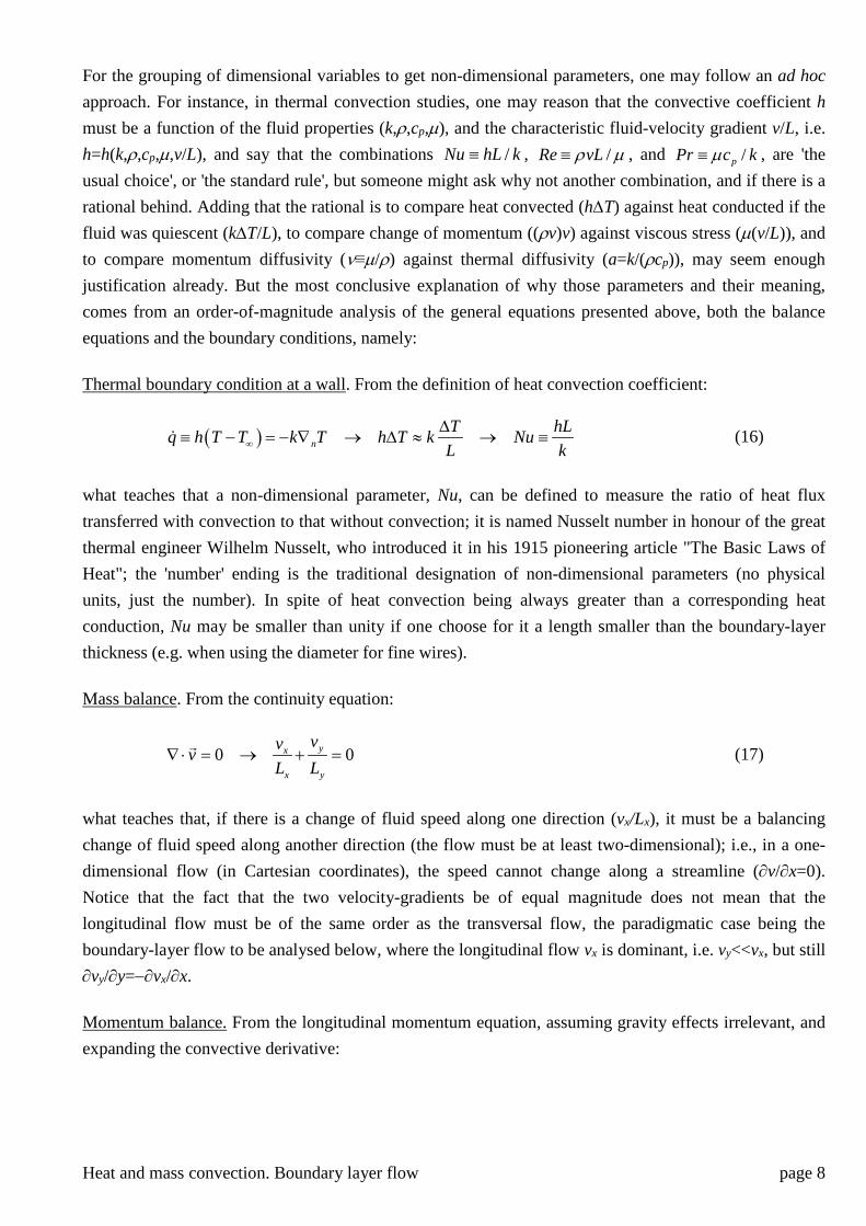
Table 1. Main non-dimensional parameters in convective heat transfer. Parameter Definition Meaning

Nusselt number hLNuk

≡ Ratio of convective heat flux to conductive heat flux.

Prandtl number Praν

≡ Ratio of momentum diffusivity to thermal diffusivity. Also, thickness ratio between velocity-boundary-layer and thermal-boundary-layer.

Reynolds number vLReν

≡ Ratio of flow convection-inertia stress to viscous stress.

Grashof number 3

2

g TLGr αν∆

≡ Ratio of fluid-buoyancy stress to viscous stress.

Rayleigh number 3

Prg TLRa Gra

αν∆

≡ = Ratio of fluid-buoyancy stress to viscous and thermal stresses.

Peclet number vLPe RePra

= = Ratio of flow convection-inertia stress to viscous and thermal stresses.

Stanton number h NuStvc Re Prρ

= = Ratio of heat convection to flow thermal capacity.

Strouhal number LSr

vω

= Ratio of flow convection-inertia stress to viscous stress.

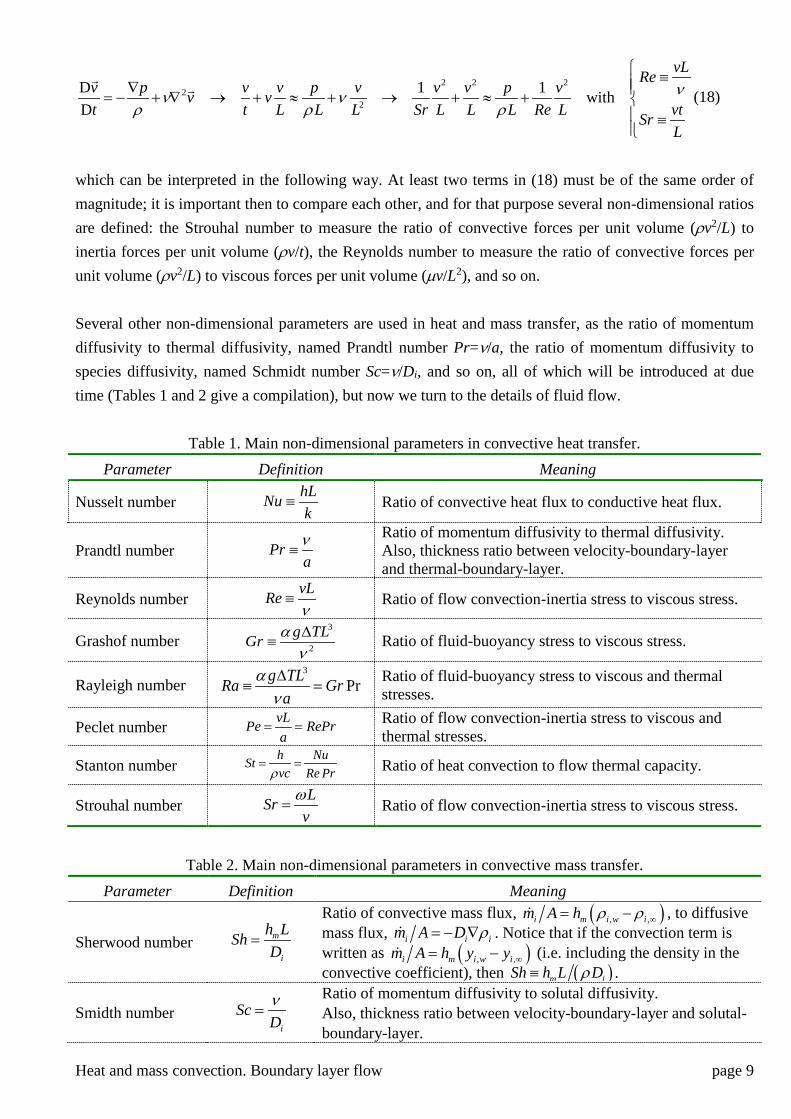
Table 2. Main non-dimensional parameters in convective mass transfer.

Parameter Definition Meaning

Sherwood number m

i

h LShD

=

Ratio of convective mass flux, ( ), ,i m i w im A h ρ ρ ∞= − , to diffusive mass flux, i i im A D ρ= − ∇ . Notice that if the convection term is written as ( ), ,i m i w im A h y y ∞= − (i.e. including the density in the convective coefficient), then ( )m iSh h L Dρ≡ .

Smidth number i

ScDν

= Ratio of momentum diffusivity to solutal diffusivity. Also, thickness ratio between velocity-boundary-layer and solutal-boundary-layer.


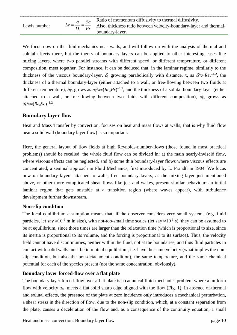
Lewis number i

a ScLeD Pr

= = Ratio of momentum diffusivity to thermal diffusivity. Also, thickness ratio between velocity-boundary-layer and thermal-boundary-layer.

We focus now on the fluid-mechanics near walls, and will follow on with the analysis of thermal and solutal effects there, but the theory of boundary layers can be applied to other interesting cases like mixing layers, where two parallel streams with different speed, or different temperature, or different composition, meet together. For instance, it can be deduced that, in the laminar regime, similarly to the thickness of the viscous boundary-layer, δ, growing parabolically with distance, x, as δ/x≈Rex−1/2, the thickness of a thermal boundary-layer (either attached to a wall, or free-flowing between two fluids at different temperature), δT, grows as δT/x≈(RexPr)−1/2, and the thickness of a solutal boundary-layer (either attached to a wall, or free-flowing between two fluids with different composition), δS, grows as δS/x≈(RexSc)−1/2.

Boundary layer flow

Heat and Mass Transfer by convection, focuses on heat and mass flows at walls; that is why fluid flow near a solid wall (boundary layer flow) is so important. Here, the general layout of flow fields at high Reynolds-number-flows (those found in most practical problems) should be recalled: the whole fluid flow can be divided in: a) the main nearly-inviscid flow, where viscous effects can be neglected, and b) some thin boundary-layer flows where viscous effects are concentrated; a seminal approach in Fluid Mechanics, first introduced by L. Prandtl in 1904. We focus now on boundary layers attached to walls; free boundary layers, as the mixing layer just mentioned above, or other more complicated shear flows like jets and wakes, present similar behaviour: an initial laminar region that gets unstable at a transition region (where waves appear), with turbulence development further downstream.

Non-slip condition The local equilibrium assumption means that, if the observer considers very small systems (e.g. fluid particles, let say ≈10-6 m in size), with not-too-small time scales (let say ≈10-3 s), they can be assumed to be at equilibrium, since those times are larger than the relaxation time (which is proportional to size, since its inertia is proportional to its volume, and the forcing is proportional to its surface). Thus, the velocity field cannot have discontinuities, neither within the fluid, not at the boundaries, and thus fluid particles in contact with solid walls must be in mutual equilibrium, i.e. have the same velocity (what implies the non-slip condition, but also the non-detachment condition), the same temperature, and the same chemical potential for each of the species present (not the same concentration, obviously).

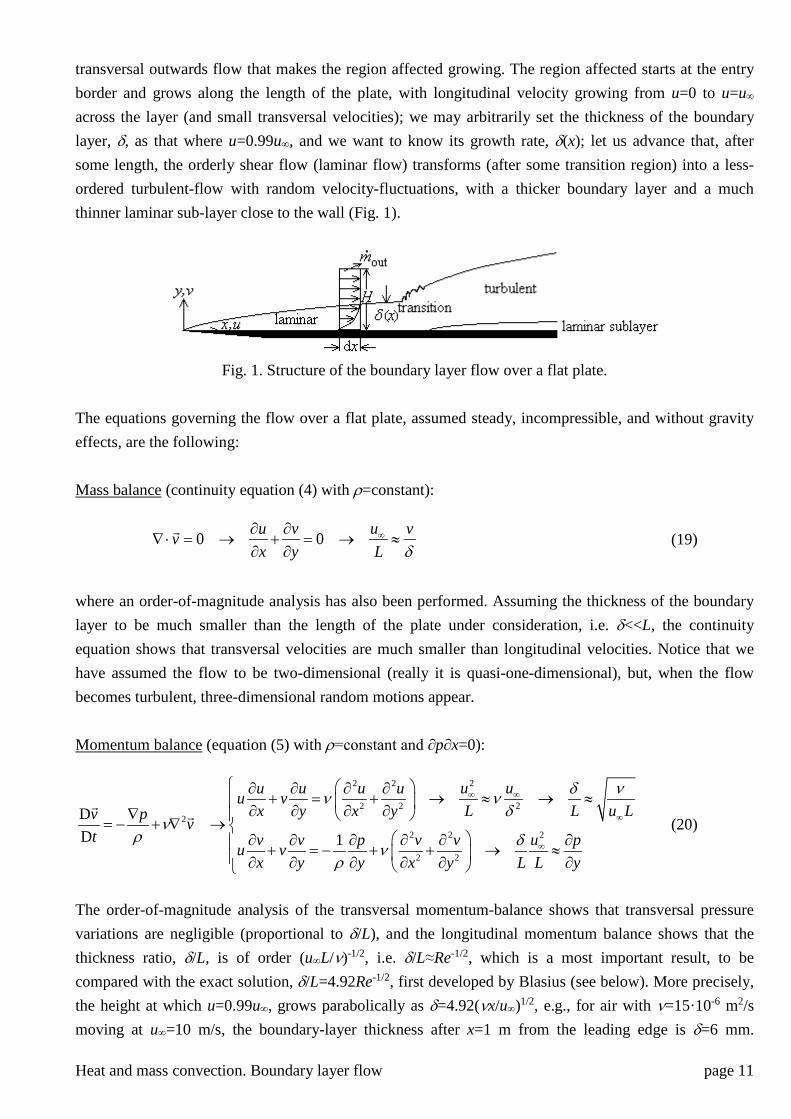
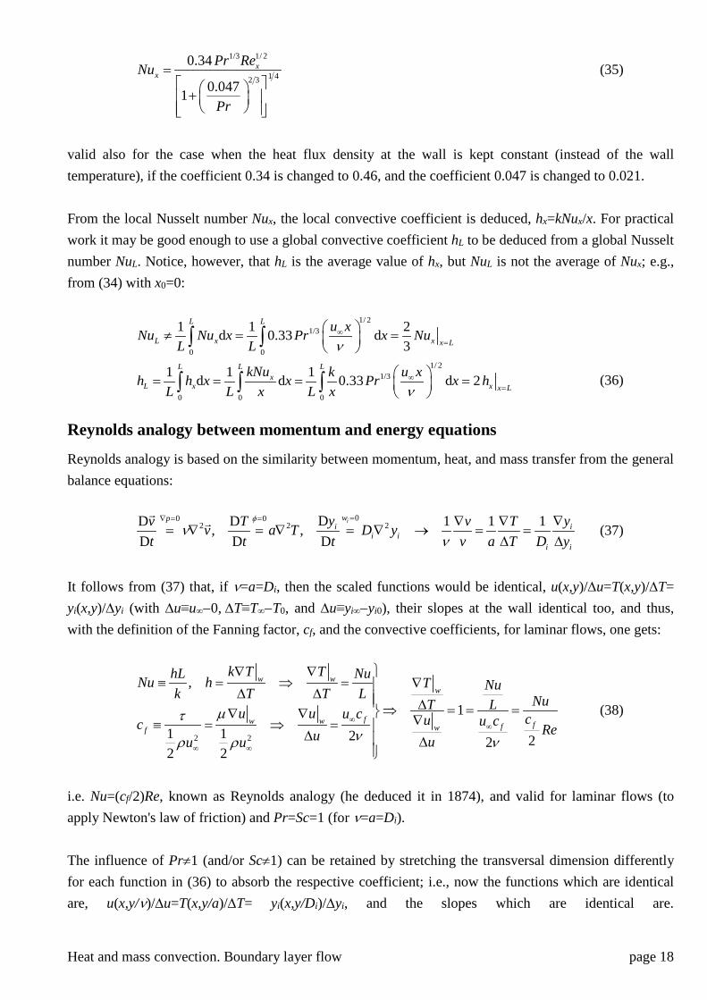
Boundary layer forced-flow over a flat plate The boundary layer forced-flow over a flat plate is a canonical fluid-mechanics problem where a uniform flow with velocity u∞, meets a flat solid sharp edge aligned with the flow (Fig. 1). In absence of thermal and solutal effects, the presence of the plate at zero incidence only introduces a mechanical perturbation, a shear stress in the direction of flow, due to the non-slip condition, which, at a constant separation from the plate, causes a deceleration of the flow and, as a consequence of the continuity equation, a small


transversal outwards flow that makes the region affected growing. The region affected starts at the entry border and grows along the length of the plate, with longitudinal velocity growing from u=0 to u=u∞ across the layer (and small transversal velocities); we may arbitrarily set the thickness of the boundary layer, δ, as that where u=0.99u∞, and we want to know its growth rate, δ(x); let us advance that, after some length, the orderly shear flow (laminar flow) transforms (after some transition region) into a less-ordered turbulent-flow with random velocity-fluctuations, with a thicker boundary layer and a much thinner laminar sub-layer close to the wall (Fig. 1).

Fig. 1. Structure of the boundary layer flow over a flat plate.

The equations governing the flow over a flat plate, assumed steady, incompressible, and without gravity effects, are the following: Mass balance (continuity equation (4) with ρ=constant):

0 0 uu v vvx y L δ

∞∂ ∂∇ ⋅ = → + = → ≈

∂ ∂ (19)

where an order-of-magnitude analysis has also been performed. Assuming the thickness of the boundary layer to be much smaller than the length of the plate under consideration, i.e. δ<<L, the continuity equation shows that transversal velocities are much smaller than longitudinal velocities. Notice that we have assumed the flow to be two-dimensional (really it is quasi-one-dimensional), but, when the flow becomes turbulent, three-dimensional random motions appear. Momentum balance (equation (5) with ρ=constant and ∂p∂x=0):

22 2

2 2 22

22 2

2 2

DD 1

u uu u u uu vx y x y L L u Lv p v

t uv v p v v pu vx y y x y L L y

δ νν νδ

νρ δν

ρ

∞ ∞

∞

∞

∂ ∂ ∂ ∂+ = + → ≈ → ≈ ∂ ∂ ∂ ∂∇ = − + ∇ →

∂ ∂ ∂ ∂ ∂ ∂ + = − + + → ≈ ∂ ∂ ∂ ∂ ∂ ∂

(20)

The order-of-magnitude analysis of the transversal momentum-balance shows that transversal pressure variations are negligible (proportional to δ/L), and the longitudinal momentum balance shows that the thickness ratio, δ/L, is of order (u∞L/ν)-1/2, i.e. δ/L≈Re-1/2, which is a most important result, to be compared with the exact solution, δ/L=4.92Re-1/2, first developed by Blasius (see below). More precisely, the height at which u=0.99u∞, grows parabolically as δ=4.92(νx/u∞)1/2, e.g., for air with ν=15·10-6 m2/s moving at u∞=10 m/s, the boundary-layer thickness after x=1 m from the leading edge is δ=6 mm.


Another consequence of (20) can be found applicable to the wall vicinity: since u|y=0=0, thence µ∂2u/∂y2|y=0=∂p∂x (equal zero for a flat plate), for both the laminar and the turbulent cases! One of Prandtl's students, P. Blasius, found in 1908 the exact solution by introducing a self-similar variable, η≡y(u∞/(νx))1/2, that transforms the PDE-system into an ordinary differential equation in the auxiliary function (the stream function, such that u=∂ψ/∂y and v=−∂ψ/∂x), ψ(η)=(u∞xν)1/2f(η), with f(η)≡∫(u/u∞)dη, the equation being:

3 2

3 2 00

d d d d2 0, with 0, 0, 1d d d d

f f f ff fη

η ηη η η η== =∞

+ = = = = (21)

which, although not analytically integrable, has a universal solution easily computed numerically, and shown in Fig. 2. The longitudinal speed fraction u/u∞=∂f/∂η asymptotically grows from 0 at the plate to 1 at infinity, attaining a precise value of 0.99 for η=4.92 (sometimes rounded to η=5, where u/u∞=0.992). Instead of the exact solution to the boundary-layer equations, an integral approximation may be good enough, i.e., a solution to integral forms of the mass and momentum equations (first developed by von Kármán in 1946), instead of a detailed solution at each point. Let u/u∞=f(y/δ) be the proposed fitting function (with δ(x) the unknown thickness), already verifying the boundary conditions f(0)=0, f(1)=1, and f'(1)=0); another condition may be added, because the longitudinal momentum equation (20) at y=0 is 0=∂2u/∂y2, as said above, and thus f''(0)=0, but this is not much important. The integrated equations are obtained for the rectangular control volume of width dx and height H sketched in Fig. 1:

( )

( )

( )

out ( ) ( )0 2( )

0 02 2 0out

0 0

dd ( ) ,d d dd d

d ddd ( ) ,d

x

x x

xy

y

m u y u H x m mx uu y uu y

x x yup u y u H x p m ux y

δ

δ δ

δ

ρ ρ δ

ρ ρ µρ ρ δ µ

∞

∞=

∞ ∞=

= + − =

∂ = − ∂∂ = + − = − ∂

∫∫ ∫

∫

(22)

which can be more explicitly formulated in terms of f≡u/u∞ and η≡y/δ(x) as:

( )( ) ( )( ) 1

20 0 00

d d d d d1 2 1d d d d d

x

y

f f ff f dy f dx u y x u

δ

η

ν δ νη ηη δ η∞ ∞ ==

− = ⇒ − =

∫ ∫ (23)

Now, an explicit f(η) will yield an explicit δ(x) from (23). For instance, if we try the simplest polynomial verifying the three boundary conditions above, f=2η−η2 (i.e. u/u∞=2(y/δ)−(y/δ)2), we get the differential equation (2/15)δ/dx=2ν/(u∞δ), which, with the condition δ(0)=0 (the layer starts at the leading edge), finally yields the result sought: δ(x)=(30νx/u∞)1/2, i.e. the boundary-layer-thickness grows parabolically with the distance to the edge. We can now found the un-stretched longitudinal velocity field, u(x,y)=u∞(2y/δ(x)−(y/δ(x))2), the longitudinal velocity slope at the wall, ∂u/∂y|y=0=(u∞/δ)∂f/∂η|η=0=2(u∞/δ)=2u2

∞/(30νxu∞)1/2, the wall shear stress τ=µ∂u/∂y|y=0, and the drag


coefficient, cf, is defined by τ=cfρu∞2/2, which is cf=(4/301/2)/(u∞x/ν)1/2. The transversal velocity profile can be found from continuity equation (19) as v(x,y)=∫−(∂u/∂x)dy=(5/6)1/2u∞(u∞x/ν)−1/2(3η2−2η3). If we add the fourth boundary condition stated above, ∂2u/∂y2|y=0=0, we need a cubic polynomial, which is f=(3η−η3)/2, and new explicit values can be found as just shown.. Table 3 gives a summary of those results, and Fig. 2 the corresponding velocity profiles. Notice, by the way, that the transversal velocity v(y) at a stage x grows in a S-shape from 0 (with dv/dy=0) to a maximum v(δ)=0.86u∞/(Rex)1/2 (0.86 for Blasius solution; 0.91=(5/6)1/2 with the simple fitting above), and remains with that value outside the boundary layer, contrary to some intuitive reasoning telling that it should vanished outside the boundary layer in the undisturbed flow; the explanation is that, with the incompressible fluid model, there is no undisturbed flow, the perturbations travelling in all directions instantaneously, and the outm contribution always exists (in reality, the whole boundary-layer model relies on the δ<<x assumption, not valid near the leading edge and far outside the boundary layer).

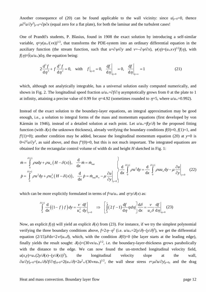
Table 3. Comparison of different solutions to the laminar boundary layer flow over a flat plate. Code (*)

Solution, f f≡u/u∞

Thickness coeff., a, in δ/x≡a/Rex

1/2 Slope coeff., b, in ∂u/∂y≡bRex

1/2u∞/x Friction coeff.,** c, in cf,x=c/Rex

1/2 Coeff.,d, in

v∞/u∞=d/Rex1/2

4 2(y/δ)−(y/δ)2 30 =5.48

2 15 =0.365

4 30 =0.730

5 6 =0.913

1 (3(y/δ)−(y/δ)3)/2 3640 13 =4.64

117 1120 =0.323

117 280 =0.646

315 416 =0.870

2 sin(π(y/δ)/2) 2 (4 )π π− =4.80

( )4 8π− =0.328

(4 ) 2π− =0.655

( )2 8 2π π− − =0.871

3 Exact sol.. (21) 4.92*** 0.332 0.664 0.86 *Codes for Fig. 2. **Defined from τ=µ∂u/∂y|y=0=cfρu∞2/2. ***Exact solution when u/u∞=0.99 (it extends from y=0 to ∞, whereas the others extend from y=0 to δ); in many books, this 4.92 is rounded to 5.0.

Fig. 2. Non-dimensional velocity profiles inside the boundary layer. Four models are shown for the

longitudinal velocity profile, u(x,y) (see details in Table 3), and only the exact profile for the transversal velocity profile, v(x,y), with Rex≡u∞x/ν.


Notice that the choice of reference frame modifies the expression of the velocity profile, and, for instance, the profile u/u∞=2(y/δ)−(y/δ)2 (number 4 in Fig. 2) refers to the origin at the plate, whereas if the origin is set at the free-end of the boundary layer, the same profile would read u/u∞=1−(y/δ)2. By the way, the latter origin is more convenient for fully-developed flow in pipes and two-dimensional ducts, where the boundary layers meet at the centre and, with the origin there, the expression u/u0=1−(y/δ)2 is valid for the whole duct; notice the change from u∞ to u0, the speed at the centre line, which is (3/2)-times the average speed in two-dimensional ducts, and twice the average speed in circular pipes. This parabolic velocity profile (named Poiseuille flow) becomes more uniform in turbulent flow, where it can be approximated by a higher-power law u/u∞=1−(y/δ)n with n between 6 an 10 (n=7 is the most common). Besides the normal boundary-layer thickness defined with u(y)=0.99u∞, two other related variables are sometimes used to quantify boundary-layer thickness: the displacement thickness δ*(x) defined by

( ) ( )* 1 ( )u u u y dyδ ∞ ∞≡ −∫ , and the momentum thickness θ(x) defined by ( ) ( )21 ( ) ( )u u y u u y dyθ ∞ ∞≡ −∫ . For a laminar boundary layer over a flat plate with no pressure gradient, δ*≈δ/3 and θ ≈2δ/15. All the models developed above, only apply to laminar boundary layer flow over a flat plate. In practice, there is an initial length with laminar flow for both sharp and rounded blunt leading edges (i.e. provided there is not flow separation at the edge), followed on by a transition region starting at some x such that Rex=(0.3..1)·106 (with very smooth plates, laminar flows up to Rex=3·106 have been achieved), and finally ending in a turbulent flow downstream. For most engineering problems it is assumed that the transition region is abrupt, and that the laminar region spans from x=0 to x=0.5·106·ν/u∞ (corresponding to a standard critical value of Re=0.5·106), and the turbulent one starts there and extends beyond (it actually depends on plate roughness and turbulence level of the entry-flow. Turbulent thickness cannot be analytically modelled (cross-coupling velocity terms appear in the momentum equation, Newton's law of friction τ=µ∂u/∂y|y=0 is no longer valid, and so on), and empirical correlations, based on the momentum-energy Reynolds analogy (explained below), are used; traditional correlations are presented in Table 4, in comparison with their laminar counterparts. Table 4. Comparison of laminar boundary-layer characteristics model with turbulent ones (see Table 3).

Velocity profile Layer thickness Friction coefficient* Laminar** Rex<0.5·106

2

1u yu δ∞

= −

1 2

4.92

xx Reδ

= f, f,1 2 1 2

0.66 1.33,x Lx L

c cRe Re

= =

Turbulent*** 0.5·106<Rex<10·106

7

1u yu δ∞

= −

1 5

0.38

xx Reδ

= f, f,1 5 1 5

0.059 0.074,x Lx L

c cRe Re

= =

*Local friction coefficient is defined by τ(x)=cf,xρu∞2/2, whereas global friction coefficient is defined by (1/L)∫τ(x)dx=cf,Lρu∞2/2. **Blasius laminar velocity profile code 4 in Table 3 and Fig. 2, but with exact coefficients for δ and cf. Notice the change of y-coordinate origin and sense from Table 3 and Fig. 2. ***Prandtl turbulent model as calibrated by Schlichting; x-coordinate origin at transition point.

Notice that turbulent thickness (Table 4) is not defined so precisely as laminar thickness, where the separation at which u(y)=0.99u∞, is neat; in turbulent boundary layers, large eddies are created and burst,


causing typical protuberances up to 1.2δ and depressions down to 0.5δ. In any case, it can be concluded that turbulent thickness is always larger than laminar thickness and grows quicker. Laminar-to-turbulent transition (LTT) depends a lot in the pressure gradient in non-flat surfaces (to be studied aside); even more, there can be a turbulent-to-laminar transition in the strongly favourable pressure gradient that occurs in a converging nozzle (relaminarization). A general warning on using empirical correlations is to be careful about the application range: all empirical correlations are limited in scope, and the most accurate, the narrower their applicability range.

Thermal boundary layer and solutal boundary layer in a forced-flow over a flat plate Analogous to the velocity boundary layer due to the jump from the non-slip condition to the free-stream flow, a thermal-boundary-layer appears if there is a difference from wall-temperature to free-flow-temperature, and a solutal boundary layer appears if there is a difference from wall-concentration of a solute to its free-flow concentration. The governing balance equations for the general case of flow-, thermal-, and solutal-boundary layers are:

0 0u vvx y

∂ ∂∇ ⋅ = → + =

∂ ∂ (24)

2

22

DD

v p u u uv u vt x y y

ν νρ

∇ ∂ ∂ ∂= − + ∇ → + =

∂ ∂ ∂

(25)

2

22

DD p

T T T Ta T u v at c x y y

φρ

∂ ∂ ∂= ∇ + → + =

∂ ∂ ∂ (26)

2

22

DD

i i i i ii i i

y w y y yD y u v Dt x y yρ

∂ ∂ ∂= ∇ + → + =

∂ ∂ ∂ (27)

Boundary conditions can be layout in a similar way to the velocity boundary layer above-explained, what shows that in the case of Pr≡ν/a=1, the function (T−Tw)/(T∞−Tw) has the same shape as the already-known u/u∞ profile, and, in the case of Sc≡ν/Di=1, the function (yi−yiw)/(yi∞−yiw) has the same shape as the already-known u/u∞ profile; see Table 3 for several approximations. The main goal in heat convection is founding h (or Nu, in non-dimensional variables), which with the above thermal-boundary-layer model yields:

( )w

w0 0

w w w 0

/ /0.33

T T yfT T

y yx x

k T y x T y fq hx xh Nu ReT T T T k T T

δ

η

ηδ η

∞

− = − = =

∞ ∞ ∞ =

− ∂ ∂ ∂ ∂ ∂≡ = → ≡ = = =

− − − ∂

(28)

where the exact Blasius solution is used (see Table 3); using instead the simplest model (T−Tw)/(T∞−Tw) =u/u∞=2(y/δ)−(y/δ)2)=1−(1−y/δ)2, one gets 0.26x xNu Re= . Instead of the local Nusselt number, the global-average value over a whole plate of length L, NuL≡(1/L)∫Nuxdx=2Nux=L can be used.


As above, the turbulent case cannot be analytically solved, but the equivalence between thermal boundary-layer and velocity boundary-layer (for Pr=1), allows to compute the temperature gradient at the wall in terms of the velocity gradient at the wall, much easier to measure, what gives Nux=cfRex/2, called Reynolds analogy, although a modified Reynolds analogy, named Reynolds-Colburn or Colburn-Chilton analogy, is commonly used (see below). An entirely similar with the convection of species i in a mixture, where the mass-convection coefficient, hm, and Sherwood number, Sh, are defined in terms of the mass-flow-rate of species i at the interface, ij

, as:

( )w

w0 0

w w w 0

/ /0.33

i i

i i

yfi i iy yi m

m x xi iw i i i i i

D y x y fj h x xh Sh ReD

ρ ρρ ρ δ

η

ρ ρ ηρ ρ ρ ρ ρ ρ δ η

∞

− = − = =

∞ ∞ =

− ∂ ∂ ∂ ∂ ∂≡ = → ≡ = = =

− − − ∂

(29)

The problem now is to find the solution for the thermal boundary layer in the laminar case but for Pr≠1, and for the solutal boundary layer when Sc≠1. Besides, we may want to consider thermal or solutal convection to start somewhere downstream, at x=x0, and not precisely at the leading edge of the plate, x=0. For Pr>1, thermal diffusivity (i.e. penetration) is smaller than momentum diffusivity (a<ν), and consequently the thermal boundary layer, δT, is thinner than the velocity boundary layer, δ. Let us measure the ratio by ζ≡δT/δ. The integral method, applied before to the velocity boundary layer, for the rectangular control volume of width dx and height H sketched in Fig. 1, gives now:

( )

( )

( )

( )

out ( ) ( )20

( )0 0 02 2

out0 0

( )

out0 0

dd ( ) ,d d dd d

d ddd ( ) ,d d dd d

d ddd ( ) ,d

x

x x

xy

y

x

y

m u y u H x m mx uu y uu y

x x yup u y u H x p m ux y

ue y ue yx xTe ue y u e H x e m e k

x y

δ

δ δ

δ

δ

ρ ρ δρ ρ µ

ρ ρ δ µ

ρ ρ

ρ ρ δ

∞

∞=

∞ ∞=

∞

∞ ∞ ∞=

= + − =

∂= − ∂∂ = + − = − ∂ =

∂ = + − = −∂

∫∫ ∫

∫

∫

( ) ( )

0 0 0

x x

y

Tky

δ δ

=

∂ − ∂ ∫ ∫

(30) Using the simplest approximation u/u∞=f(η)=2(y/δ)−(y/δ)2 (see Table 3), putting energy proportional to temperature, e=cT, a corresponding profile (T−Tw)/(T∞−Tw)=2(y/δΤ)−(y/δΤ)2=f(η/ζ), and ζ≡δT/δ, one gets:

( )( ) ( ) ( )( )

( )( ) ( ) ( )T T

( ) ( )

20 00 0

( ) ( )

w0 00 0

d dd 1 dd d

d dd 1 dd d

x x

y y

x x

y y

u uu u u y f f yx y x u y

T a Tu T T y a f f yx y x u T T y

δ δ

δ δ

νν η η

ηηζ

∞∞= =

∞∞ ∞= =

∂ ∂− = − → − = − ∂ ∂

∂ ∂ − = − → − = − ∂ − ∂

∫ ∫

∫ ∫ (31)


where the energy integral is limited to δT because T−T∞ is zero outside. Performing the substitutions and integration, (31) yields:

( )( ) ( )

( ) ( ) ( ) ( )( ) ( )

( ) 2 22 3

2d 2 30d 15 d 420 6 5

d5d 2d 30 30

x xxx u x u

xx Prx x x x a

x u x x

δ ν νδδ ζζ ζ ζ ζ

ζ δ ζ δζ δ

∞ ∞

∞

− = − → =

− + − = − = −

(32)

i.e., the momentum integral gives the thickness law for the velocity boundary layer, which is substituted in the energy integral to get, either a constant δT/δ-relation if only the leading terms are kept, namely 5ζ3=4/Pr, or, if an initial condition ζ(x0)=0 is imposed:

( )0

1/33/4 01/3 1/30T 0.93 1 0.93

xxx Pr Prx

δζδ

−→

− − ≡ = − =

(33)

If, instead of model 4 (see Table 3), the more refined model 1 is used, the only changes are the change in the coefficients: δ=4.64(νx/u∞)1/2 instead of δ=5.48(νx/u∞)1/2, and 1.02 instead of 0.93 in (33). Besides the thermal thickness, the slope of the thermal profile at the wall is important; with model 4, for which we found du/dy|y=0=0.365(νxu∞)1/2, now we get, for x0=0, dT/dy|y=0=0.39(T∞−Tw)Rex

1/2Pr1/3/x, which is not too far from the most precise coefficient found by Pohlhausen in 1921 (0.33 instead of (270)−1/6=0.39). In the traditional non-dimensional form, retaining the possibility of the temperature jump starting somewhere downstream, at x=x0, one has:

1/33/4

0 1/3 1/ 2 0/

0.33 1yx x

w

x T y xhxNu Pr Rek T T x

−

=

∞

∂ ∂ ≡ = = − − (34)

Again, the global-average value of the Nusselt number over a whole plate of length L, is often used; for x0=0, NuL≡(1/L)∫Nuxdx=2Nux=L. Notice that the above result comes from a global energy balance in the whole of the thermal layer, thus, an integral average of the fluid properties must be used, and not just their values at wall conditions; these 'film averaged' values are usually computed just as the algebraic mean of the values at wall conditions and at bulk conditions (here the undisturbed conditions), i.e. Tfilm≡(Tw+T∞)/2. Pohlhausen correlation (34), although deduced for Pr>1, has been found to be accurate for 0.6<Pr<60, but not enough for the very high Prandtl numbers exhibited by some oils and silicones, and for Pr<<1 typical of liquid metals. An extension to Pohlhausen correlation in the whole range of Prandtl numbers was made by Churchill and Ozoe in 1973 in the form:


1/3 1/ 2

1 42 3

0.34

0.0471

xx

Pr ReNu

Pr

= +

(35)

valid also for the case when the heat flux density at the wall is kept constant (instead of the wall temperature), if the coefficient 0.34 is changed to 0.46, and the coefficient 0.047 is changed to 0.021. From the local Nusselt number Nux, the local convective coefficient is deduced, hx=kNux/x. For practical work it may be good enough to use a global convective coefficient hL to be deduced from a global Nusselt number NuL. Notice, however, that hL is the average value of hx, but NuL is not the average of Nux; e.g., from (34) with x0=0:

1/ 2

1/3

0 0

1 1 2d 0.33 d3

L L

L x x x L

u xNu Nu x Pr x NuL L ν

∞=

≠ = = ∫ ∫

1/ 2

1/3

0 0 0

1 1 1d d 0.33 d 2L L L

xL x x x L

kNu u xkh h x x Pr x hL L x L x ν

∞=

= = = = ∫ ∫ ∫ (36)

Reynolds analogy between momentum and energy equations

Reynolds analogy is based on the similarity between momentum, heat, and mass transfer from the general balance equations:

00 0

2 2 2DD D 1 1 1, ,D D D

iwpi i

i ii i

y yv T v Tv a T D yt t t v a T D y

φ

νν

=∇ = = ∇∇ ∇= ∇ = ∇ = ∇ → = =

∆ ∆

(37)

It follows from (37) that, if ν=a=Di, then the scaled functions would be identical, u(x,y)/∆u=T(x,y)/∆T= yi(x,y)/∆yi (with ∆u≡u∞−0, ∆T≡T∞−T0, and ∆u≡yi∞−yi0), their slopes at the wall identical too, and thus, with the definition of the Fanning factor, cf, and the convective coefficients, for laminar flows, one gets:

2 2

,

1

1 1 2 222 2

w ww

fw w ffwf

k T ThL NuNu h T Nuk T T L NuT Lu u u c cu u cc Reu uu u

µτν νρ ρ

∞∞

∞ ∞

∇ ∇ ≡ = ⇒ = ∇∆ ∆ ∆⇒ = = =∇ ∇ ∇≡ = ⇒ =

∆ ∆

(38)

i.e. Nu=(cf/2)Re, known as Reynolds analogy (he deduced it in 1874), and valid for laminar flows (to apply Newton's law of friction) and Pr=Sc=1 (for ν=a=Di). The influence of Pr≠1 (and/or Sc≠1) can be retained by stretching the transversal dimension differently for each function in (36) to absorb the respective coefficient; i.e., now the functions which are identical are, u(x,y/ν)/∆u=T(x,y/a)/∆T= yi(x,y/Di)/∆yi, and the slopes which are identical are.


∇u(x,y/ν)/∆u=ν∇u(x,y)/∆u= ∇T(x,y/a)/∆T=a∇T(x,y)/∆T= ∇yi(x,y/Di)/∆yi=Di∇yi(x,i)/∆yi, Thence, (38) becomes:

2 2

,

1

1 1 2 2 22 2

w ww

fw w f fwf

k T ThL NuNu h a a T Nuk T T L a a NuT Lu u u c u c cuc Re Pru uu u

µτ ν ν ννν νρ ρ

∞∞

∞ ∞

∇ ∇ ≡ = ⇒ = ∇∆ ∆ ∆ = = =∇ ∇ ∇≡ = ⇒ =

∆ ∆

(39)

i.e. Nu=(cf/2)RePr. However, if we compare the exact solutions to the laminar boundary layer obtained above (Eq. (34) and Table 4), we obtained a more accurate Pr-correction to Reynolds analogy:

0 01/3 1/ 2

,f, 1/32/3

f, 1 2

0.330.66 2 2

x

x x f xx xx x

xxx

Nu Pr Re cc NuNu Re Pr StPr Re Prc

Re

= = ⇒ = ⇒ ≡ =

=

(40)

which is known as Chilton-Colburn analogy (1934); St is a combined parameter named Stanton number. Although (40) has been developed only for a laminar-boundary-layer flow over a flat plate, it applies with good accuracy to both laminar and turbulent flows over flat plates in the 0.6<Pr<60, and even to any turbulent flow with pressure gradients, but not to laminar flows with ∇p≠0 (i.e. Colburn-Chilton analogy can be applied to any turbulent flow, but only to laminar flows over flat plates, not to laminar flows in pipes or around bodies). A compilation of heat-transfer correlations in forced convection over a flat plate is presented in Table 5. A note on correlations for turbulent flow is required: the local Nusselt number Nux is used to get the local convective coefficient using hx=kNux/x with x measured from the leading edge of the plate (not from the start of the turbulent layer), whereas the global Nusselt number NuL is used to get the global convective coefficient using hL=kNuL/L which includes both the laminar zone and the turbulent zone:

tr tr

tr tr

1/ 2 4 /51/3 1/3

,lam ,turb0 0 0

1 1 1d d d 0.33 d 0.03 dx xL L L

L x x xx x

u x u xk kh h x h x h x Pr x Pr xL L L x xν ν

∞ ∞ = = + = + =

∫ ∫ ∫ ∫ ∫

( ) ( )( )6tr

1/3 1/30.5 101/ 2 4 /5 4 /5 4 /5

tr tr52 0.33 0.030 467 0.037 362004

ReL L L

k Pr k PrRe Re Re h ReL L

= ⋅ = ⋅ + − → = + − =

( )1/3

4 /50.037 870L Lk Prh Re

L= − (41)

Table 5. Heat transfer correlations in forced convection over a flat plate.

Flow regime Correlation Laminar

Rex<Retr=0.5·106 (i.e. x<xtr=0.5·106ν/u∞)

(coefficients shown are for constant Twall;

for constant qwall, change

If 0.6<Pr<500 (modified Pohlhausen equation): 1/33/4

1/3 1/ 2 00.33 1x xxNu Pr Rex

− = −


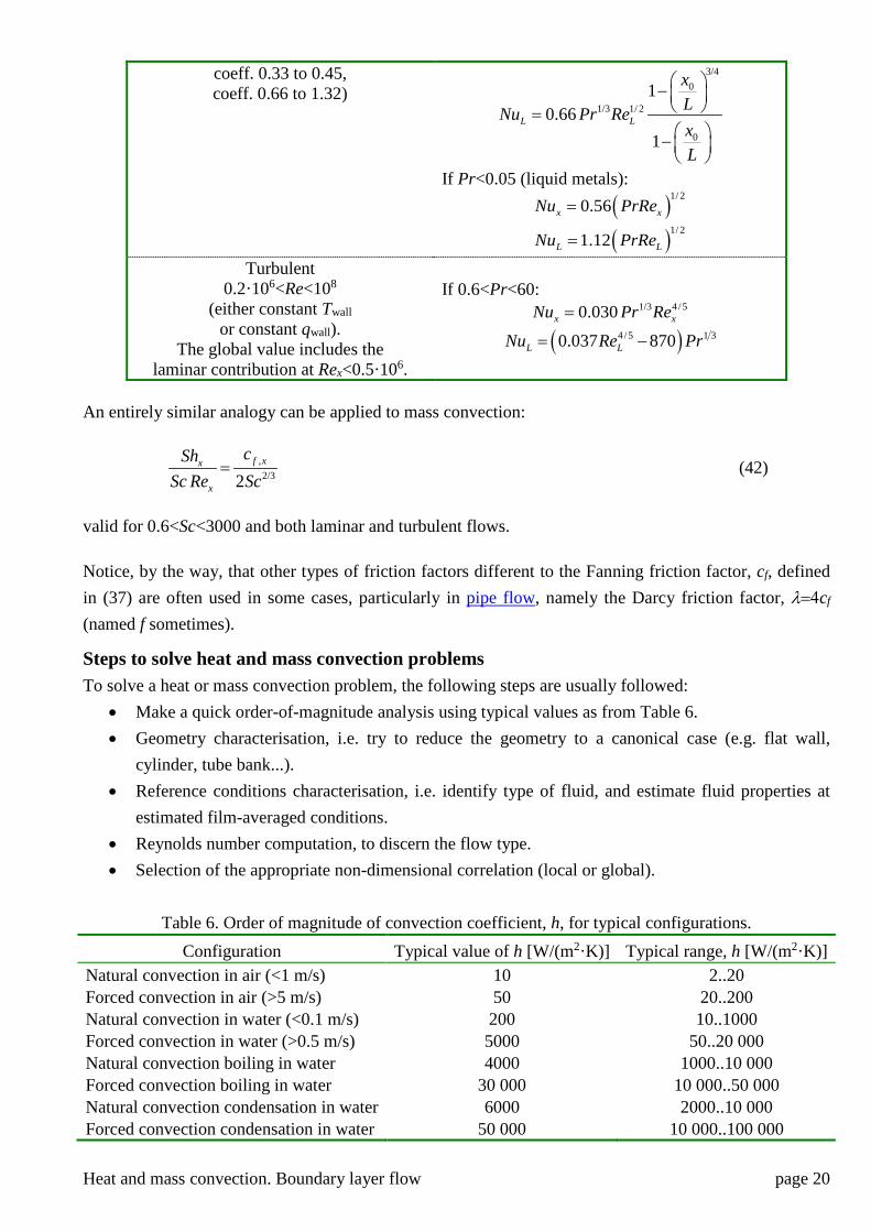
coeff. 0.33 to 0.45, coeff. 0.66 to 1.32)

3/40

1/3 1/ 2

0

10.66

1L L

xLNu Pr RexL

− = −

If Pr<0.05 (liquid metals):

( )1/ 20.56x xNu PrRe=

( )1/ 21.12L LNu PrRe=

Turbulent 0.2·106<Re<108

(either constant Twall or constant qwall).

The global value includes the laminar contribution at Rex<0.5·106.

If 0.6<Pr<60: 1/3 4/50.030x xNu Pr Re=

( )4/5 1 30.037 870L LNu Re Pr= −

An entirely similar analogy can be applied to mass convection:

,2/32

f xx

x

cShSc Re Sc

= (42)

valid for 0.6<Sc<3000 and both laminar and turbulent flows. Notice, by the way, that other types of friction factors different to the Fanning friction factor, cf, defined in (37) are often used in some cases, particularly in pipe flow, namely the Darcy friction factor, λ=4cf (named f sometimes).

Steps to solve heat and mass convection problems To solve a heat or mass convection problem, the following steps are usually followed:

• Make a quick order-of-magnitude analysis using typical values as from Table 6. • Geometry characterisation, i.e. try to reduce the geometry to a canonical case (e.g. flat wall,

cylinder, tube bank...). • Reference conditions characterisation, i.e. identify type of fluid, and estimate fluid properties at

estimated film-averaged conditions. • Reynolds number computation, to discern the flow type. • Selection of the appropriate non-dimensional correlation (local or global).

Table 6. Order of magnitude of convection coefficient, h, for typical configurations.

Configuration Typical value of h [W/(m2·K)] Typical range, h [W/(m2·K)] Natural convection in air (<1 m/s) 10 2..20 Forced convection in air (>5 m/s) 50 20..200 Natural convection in water (<0.1 m/s) 200 10..1000 Forced convection in water (>0.5 m/s) 5000 50..20 000 Natural convection boiling in water 4000 1000..10 000 Forced convection boiling in water 30 000 10 000..50 000 Natural convection condensation in water 6000 2000..10 000 Forced convection condensation in water 50 000 10 000..100 000



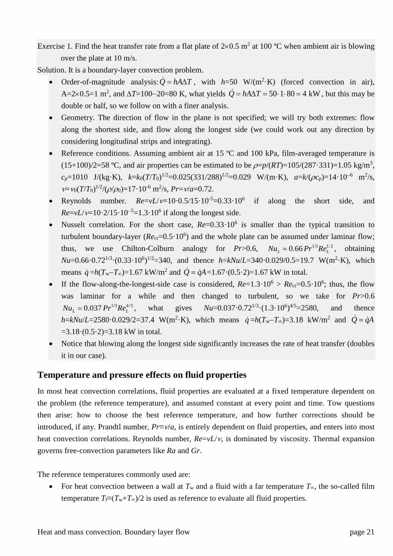
Exercise 1. Find the heat transfer rate from a flat plate of 2×0.5 m2 at 100 ºC when ambient air is blowing

over the plate at 10 m/s. Solution. It is a boundary-layer convection problem.

• Order-of-magnitude analysis: Q hA T= ∆ , with h=50 W/(m2·K) (forced convection in air), A=2×0.5=1 m2, and ∆T=100−20=80 K, what yields 50 1 80 4 kWQ hA T= ∆ = ⋅ ⋅ = , but this may be double or half, so we follow on with a finer analysis.

• Geometry. The direction of flow in the plane is not specified; we will try both extremes: flow along the shortest side, and flow along the longest side (we could work out any direction by considering longitudinal strips and integrating).

• Reference conditions. Assuming ambient air at 15 ºC and 100 kPa, film-averaged temperature is (15+100)/2=58 ºC, and air properties can be estimated to be ρ=p/(RT)=105/(287·331)=1.05 kg/m3, cp=1010 J/(kg·K), k=k0(T/T0)1/2=0.025(331/288)1/2=0.029 W/(m·K), a=k/(ρcp)=14·10−6 m2/s, ν=ν0(T/T0)1/2/(ρ/ρ0)=17·10-6 m2/s, Pr=ν/a=0.72.

• Reynolds number. Re=vL/ν=10·0.5/15·10-5=0.33·106 if along the short side, and Re=vL/ν=10·2/15·10−5=1.3·106 if along the longest side.

• Nusselt correlation. For the short case, Re=0.33·106 is smaller than the typical transition to turbulent boundary-layer (Recr=0.5·106) and the whole plate can be assumed under laminar flow; thus, we use Chilton-Colburn analogy for Pr>0.6, 1/3 1/ 20.66L LNu Pr Re= , obtaining Nu=0.66·0.721/3·(0.33·106)1/2=340, and thence h=kNu/L=340·0.029/0.5=19.7 W(m2·K), which means q =h(Tw−T∞)=1.67 kW/m2 and Q qA= =1.67·(0.5·2)=1.67 kW in total.

• If the flow-along-the-longest-side case is considered, Re=1.3·106 > Recr=0.5·106; thus, the flow was laminar for a while and then changed to turbulent, so we take for Pr>0.6

1/3 4/50.037L LNu Pr Re= , what gives Nu=0.037·0.721/3·(1.3·106)4/5=2580, and thence h=kNu/L=2580·0.029/2=37.4 W(m2·K), which means q =h(Tw−T∞)=3.18 kW/m2 and Q qA=

=3.18·(0.5·2)=3.18 kW in total. • Notice that blowing along the longest side significantly increases the rate of heat transfer (doubles

it in our case).

Temperature and pressure effects on fluid properties

In most heat convection correlations, fluid properties are evaluated at a fixed temperature dependent on the problem (the reference temperature), and assumed constant at every point and time. Tow questions then arise: how to choose the best reference temperature, and how further corrections should be introduced, if any. Prandtl number, Pr≡ν/a, is entirely dependent on fluid properties, and enters into most heat convection correlations. Reynolds number, Re=vL/ν, is dominated by viscosity. Thermal expansion governs free-convection parameters like Ra and Gr. The reference temperatures commonly used are:

• For heat convection between a wall at Tw and a fluid with a far temperature T∞, the so-called film temperature Tf≡(Tw+T∞)/2 is used as reference to evaluate all fluid properties.


• For heat convection in a pipe, the most appropriate temperature reference is the inlet-and-outlet bulk average, although, when the outlet is unknown, the inlet mean temperature-difference between the fluid and pipe wall is used as reference.

From the several fluid properties involved in heat convection without phase change (density, ρ, viscosity, µ, thermal conductivity, k, thermal capacity, cp, thermal expansion coefficient, α, and so on), viscosity of liquids is the most sensitive to temperature variations, all the others being mildly dependent on temperature and pressure. Gases

• Density. Density in gases can usually be computed from ideal gas law ρ=p/(RT) without any other correction. Temperature affects almost all gas properties. Pressure, if not below 102 Pa, has a negligible effect on cp, k, and µ (and on Pr≡µcp/k), but the Reynolds number is almost proportional to gas pressure (Re≡vL/ν ∝ p), and Rayleigh number, Ra≡αg∆TL3/(να), proportional to p2 (and hence the convective coefficient in natural convection is proportional to the square root of pressure, h=h0 0p p ). For p<102 Pa the continuum model starts to fail, and for p<101 Pa the molecular mean free path becomes comparable or larger than the size of the object of interest, and kinetic gas theory must be applied.

• Thermal capacity. Slowly increases with temperature (polynomial fittings are common); e.g. for air at 100 kPa, cp=1032 J/(kg·K) at 100 K and cp=1141 J/(kg·K) at 1000 K.

• Thermal conductivity and dynamic viscosity. This two transport coefficients increase with temperature with a small power-law (k=k0(T/T0)n and µ=µ0(T/T0)m); although kinetic theory of gases show that both, thermal conductivity and dynamic viscosity, grow with T1/2, a linear fit better fits the data. For more precise correlations, the following exponents have been proposed: n=0.71 and m=0.65 for monatomic gases, n=0.86 and m=0.70 for diatomic gases, n=1.3 and m=0.88 for triatomic gases. Both transport coefficients are nearly unchanged by pressure up to 10 MPa, increasing to a double value at some 50 MPa.

• Thermal diffusivity. A general dependence with temperature and pressure is of the form Tn/p, with 1.5<n<2 (n=3/2 according to simple kinetic gas theory); e.g. for air at 100 kPa, a=2.54·10-6 m2/s at 100 K and a=168·10-6 m2/s at 1000 K.

• Prandtl number. Gases have a typical value of Pr=0.7 and a small temperature dependence, with 0.5<Pr<1 under most p-T-conditions; e.g. for air at 100 kPa, Pr=0.79 at 100 K and Pr=0.73 at 1000 K.

Liquids • Density. Temperature affects almost all liquid properties. The linear thermal expansion model

for the density of liquids is good enough in most cases (far from the critical-point conditions). Saturated water, for instance, has ρ=1002 kg/m3 at 0 ºC, ρ=960.6 kg/m3 at 100 ºC and ρ=322 kg/m3 at its critical point, 374 ºC. Pressure has a negligible effect on liquids (above their vapour pressure).

• Thermal capacity. May slightly increase or decrease with temperature; e.g. for saturated water, cp=4218 J/(kg·K) at 0 ºC and cp=5728 J/(kg·K) at 300 ºC.


• Viscosity. A simple temperature-corrections for liquid viscosity is:

( ) exp 1T TCT

µµ

⊕

⊕

= − −

(42)

with a constant value of around C≈7; e.g. for water, C=6, with µ⊕=0.0011 Pa·s at T⊕=288 K; for

many oils, C=8, with a typical value of (see Liquid data) µ⊕=0.1 Pa·s at T⊕=288 K, and so on. Saturated water, for instance, has ν=1.79 m2/s at 0 ºC and ν=0.135 m2/s at 300 ºC.

• Prandtl number. Most liquids, except viscous oils and liquid metals, have a range of 2<Pr<20 (e.g., at 15 ºC, Pr=7 for water, Pr=8 for n-octane, Pr=19 for ethanol), decreasing with temperature (e.g. Pr=1.02 for saturated water at 300 ºC, Pr=13.6 at 0 ºC). Viscous liquids like oils and glycerine may have large Prandtl-values, 50<Pr<105 (larger values are seldom considered as convecting), quickly decreasing when temperature is increased. Most liquids metals, under most p-T-conditions, have 0.005<Pr<0.05, with a typical value of Pr=0.01.

After having computed all fluid properties at the appropriate reference temperature, some corrections may be due, to account for the different possible temperature gradients. For gases, when the wall-to-bulk temperature ratios is in the range 0.5<Tw/T∞<2, using the film temperature is good enough. For liquids, and for gases at high wall-to-bulk temperature ratios, heat convection correlations computed with mean film temperatures are modified with a viscosity factor, as the (µw/µ∞)1/4 term in Table 5.

Forced and natural convection (aside)

Convection with phase change (aside)

Heat exchangers (aside) Back to Heat and mass transfer

Back to Thermodynamics

http://webserver.dmt.upm.es/%7Eisidoro/dat1/eLIQ.htm


http://webserver.dmt.upm.es/%7Eisidoro/bk3/c12/Convection%20with%20phase%20change.pdf

http://webserver.dmt.upm.es/%7Eisidoro/bk3/c12/Heat%20exchangers.pdf

http://webserver.dmt.upm.es/%7Eisidoro/bk3/index.html

Documents

HEAT AND MASS CONVECTION - UPM