Embed Size (px)
Citation preview

1
Heat and Mass Transfer Prof. U.N. Gaitonde
Dept. of Mechanical Engineering Indian Institute of Technology, Bombay
Lecture No. 17
Review of Fluid Mechanics – 2
Welcome back to the second lecture on the review of fluid mechanics. In the previous lecture we
looked at the basic equations governing fluid mechanics, in particular the Navier-Stokes
equations and then looked some simple situations of internal flows, particularly flow through a
pipe or a duct. Now we move on to another class of flows known as external flows.
(Refer Slide Time: 01:30)
External flow is a flow around submerged bodies and here we have a typical submerged body - an
airfoil which is confronting a free stream which is the fluid flowing and surrounding it. One of the
most important concepts for such flows around submerged bodies - also known as bluff bodies
quite often - is the boundary layer around the submerged body and many of these flows are know
as boundary layer flows.
Generally the boundary layer is a small region surrounding the submerged body and the effects of
the presence of the submerged body, particularly the viscosus effects are felt in this small region
known as the boundary layer. Whenever there is some sort of flow around a submerged body, a

2
boundary layer will come into existence. Beyond the boundary layer, you have a zone of
essentially inviscid flow in which the viscous effects caused by the boundary layer are negligible
and this flow region gets affected only by the shape of this body; it doesn’t get affected by the
shear forces which occur on the surface of the body.
It is the boundary layer concept which allows us to analyze and visualize the flow situation
around submerged bodies. Here I have shown a boundary layer around an airfoil but there are
other situations where you will come across boundary layers of different kinds.
(Refer Slide Time: 03:44)
One situation is that of a thin flat plate when it is exposed to a fluid known as the free stream. We
expect that is on one side, the fluid at sufficiently large distance from the surface for a thin plate,
they will remain at V infinity - this is the known as the free stream. However the fluid at the
surface of the plate will become stagnant because of the presence of the plane; the fluid will stick
to it and hence you will have a situation where you will have a V infinity away from the surface
as the velocity will go down to 0 at the surface.
You will notice that the surface effect is felt only up to a certain distance; near the leading edge
this effect is much thinner since as you go away from the leading edge, you find the zone in
which the velocity is lower than the free stream velocity and this layer is know as the boundary
layer. On the other side of the thin plate also you will have a symmetric boundary layer; boundary

3
layer may occur even on bodies such as a cylinder which is exposed to a fluid. Here a thin
boundary layer will develop and will go around the cylinder. Part of the boundary layer may be
laminar, part of the boundary layer may be turbulent and the boundary layer may even separate
into what is known as a wake. So here you have part of the, reaching which is the boundary layer
then we have separation leading to a wake and depending on the diameter of the cylinder V
infinity there will be different formats in different forms of the boundary layer and different
forms of the wake. As we proceed, we will some see some these situations in more detail.
(Refer Slide Time: 06:54)
It will nice to see what exactly is meant by a boundary layer. Boundary layer typically has 3
characteristics; one characteristic is that it is a thin layer, by thin we mean comparable to the
dimensions of the plate. Looking back here, we expect this thickness of the boundary layer to be
much smaller than the length of the plate. If the length of the plate is of the order of a meter, the
thickness of the boundary layer is likely to be of the order of a millimeter or so. On large bodies
like an aircraft wing with a width of may be a few meters, the boundary layer will be perhaps of
the order of a few millimeters or a few centimeters.
The second characteristic of a boundary layer is that the component normal to the layer is small
compare to the component parallel to the boundary layer.

4
(Refer Slide Time: 08:09)
If I show a boundary layer again on a flat plate, let us say this is the boundary layer; in the
boundary layer the component Vx and the component Vy will have magnitude such that Vy is
much smaller is then Vx. So there a major and predominant direction of flow along the length of
the boundary layer though component of velocity perpendicular across the boundary layer will be
much smaller than Vx; so here Vy that is much smaller Vx.
The third characteristic is that the gradients of any variable x, component of velocity y,
component of velocity, even pressure along the direction of flow are small compared to across the
direction of flow. So for example, if in the same boundary layer I take say the velocity profile.
This is Vx so it reduces from V infinity in the free steam to 0 at the wall and this is the function of
y at a particular x but at a different x, Vx will have different values even at the same y. If you
consider the variation of Vx in the y direction, that will be much larger than the variation of Vx in
the x direction since the gradients of Vx and even pressure temperature, whatever, are higher in
the perpendicular direction than in the flow direction. Conduction of heat, diffusion of
momentum would all be significant in the y direction that is across the boundary layer than along
boundary layer. This is a major characteristic of the boundary layer.
So again remember that the boundary layer has 3 basics characteristics - that it is a thin layer of
flow, thin compared to dimensions of the body surrounding which the boundary layer comes into
existence; there is a major velocity component along the direction of the boundary layer, velocity
5
component across the boundary layer is small and the gradients are significant across the
boundary layer and not along the direction of flow.
Now these characteristics particularly these significant inequalities simplify the governing
equations of fluid flow; that means the Navier-Stokes equation in the boundary layer can be
reduced to significantly simplified forms. In particular, the simplification uses the fact that the y
component of velocity is much smaller than the x component of velocity and any component of
velocity varies significantly in the y direction compared to its variation in the x direction. The
simplified Navier-Stokes equations simplified using the boundary layer approximations are
known as boundary layer equations.
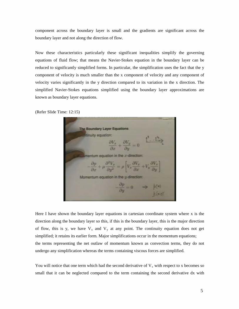
(Refer Slide Time: 12:15)
Here I have shown the boundary layer equations in cartesian coordinate system where x is the
direction along the boundary layer so this, if this is the boundary layer, this is the major direction
of flow, this is y, we have Vx and Vy at any point. The continuity equation does not get
simplified; it retains its earlier form. Major simplifications occur in the momentum equations;
the terms representing the net outlaw of momentum known as convection terms, they do not
undergo any simplification whereas the terms containing viscous forces are simplified.
You will notice that one term which had the second derivative of Vx with respect to x becomes so
small that it can be neglected compared to the term containing the second derivative dx with

6
respect to y. The momentum equation in the y direction gets so simplified that it reduces to a
form where we say that the pressure variation across the boundary layer is 0. This means that the
pressure in the boundary layer does not vary across the boundary layer; it will vary in the x
direction only. So this implies that pressure is a function only of x and not of x and y and that is
why many times the boundary layer equations are written without this equation and with this
partial derivative of pressure with respect to x replaced by now ordinary derivative of pressure
with respect to x.
Inspite of the simplification in the Navier-Stokes equation in the boundary layer, it turns out that
these equations are so, not so easy to solve. They are are easier to solve than the full Navier-
Stokes equations but they are are not very simple. So these equations can be solved only for a set
of reasonably simple situations.
(Refer Slide Time: 15:10)
And hence for most situations of practical interest and for situations in which the boundary layer
is turbulent, either the whole boundary layer is turbulent or the boundary layer is turbulent in part,
we use correlations based on experimental data. And just the way experimental data and pressure
drops, results for internal flows are converted into a dimensionless parameter called the friction
factor.

7
Here in case of boundary layer flows, for external flows the results are converted into a relation
for what is known as the drag coefficient or the skin friction coefficient. We can have a local drag
coefficient and the average local drag coefficients. The local drag coefficients will depend on the
location so Cf at x will be different for different x and average drag coefficients will be average
over a certain length. Let us look at the definition of the drag coefficient.
(Refer Slide Time: 16:22)
If we have a boundary layer, this is the velocity profile in the boundary layer and because of this
gradient of the velocity at the wall, this slope represents variation of Vx with respect to y at the
wall. There is a shear stress which is equal to mu into this gradient of Vx into the y direction
because of the viscous friction due to the finite viscosity of the fluid and this tau is converted into
the dimensionless drag coefficient or skin friction coefficient.
As we go along the length of the plate, the boundary layer thickness varies, so the gradient at the
wall varies; this will be different at different values of x, hence the shear stress will be different at
different values of x. And hence the drag coefficient will be different at different values of x.
(Refer Slide Time: 17:53)

8
The local drag coefficient is this local value of the shear stress divided by rho infinity squared by
2 which is the velocity head at V infinity which is the free stream value of the velocity. Notice
that this, I, the dimensions of pressure or force per unit area. This also is a dimension of pressure
and hence the skin friction coefficient is a dimensionless number as is the friction factors also a
dimensionless number. In practical applications we are interested in the total drag force for
which we can integrate out the shear force along the length or along the surface and get the value
at the drag force.
Based on the drag force or drag force per unit area, we can define an average skin friction
coefficient and the definition of the average skin friction coefficient would be the drag force
divided by the area of the plate divided by rho V infinity square by 2.

9
(Refer Slide Time: 19:17)
So maybe I should draw another figure; if this is the plate and on the plate the total net force
because of all the skin frictions is FD. Then take the magnitude of FD divided by A where A is the
total area of the plate - force per unit area; this is will have a dimensions of pressure divided by
rho V infinity squared by 2 where V infinity is the free stream velocity and we have our average
drag coefficient. And the average drag coefficient can be shown to be, if you have a flow in
which the variation is only along the length of the plate, it will be the average of the local skin
friction coefficient - Cfx dx integrated over the length and taken average.
The flat plate situation which we have been mentioning again and again is a basic or fundamental
flow situation. The governing Navier-Stokes equations in the boundary layer form can be with
some difficulty solved for this situation and if the flow is laminar, steady, 2-dimensional, constant
property, incompressible, then we can analytically obtain an expression for the local drag
coefficient and the average drag coefficient.
10
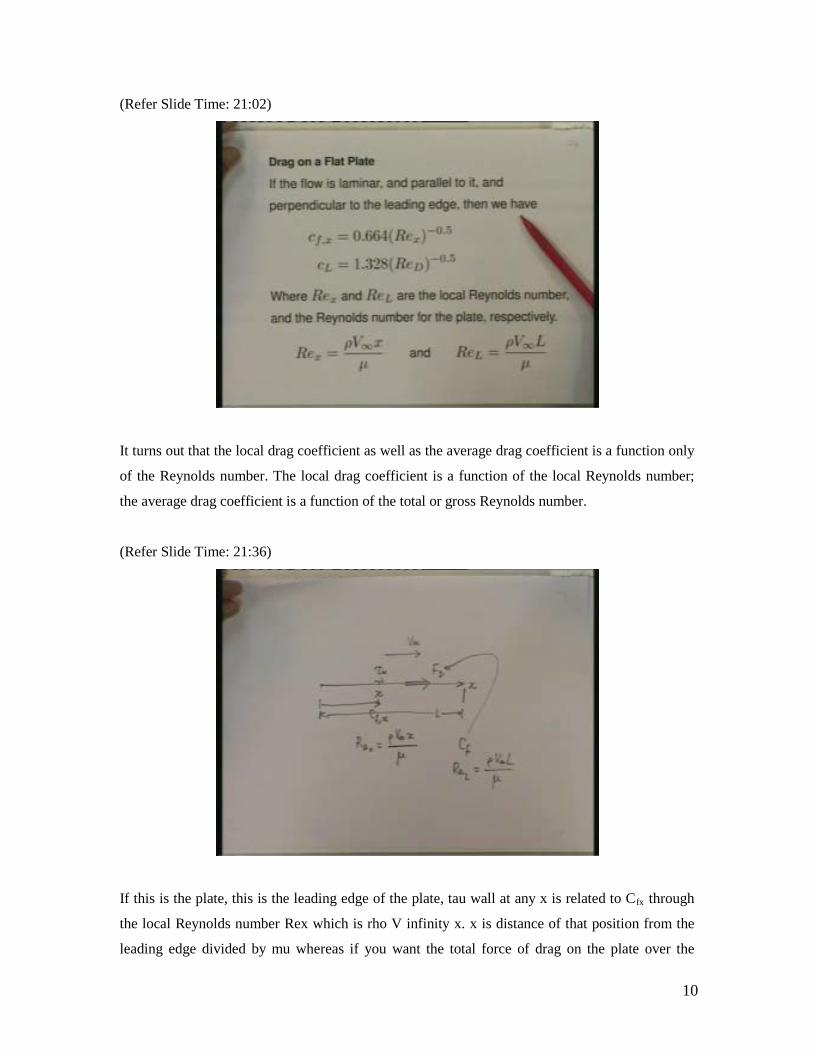
(Refer Slide Time: 21:02)
It turns out that the local drag coefficient as well as the average drag coefficient is a function only
of the Reynolds number. The local drag coefficient is a function of the local Reynolds number;
the average drag coefficient is a function of the total or gross Reynolds number.
(Refer Slide Time: 21:36)
If this is the plate, this is the leading edge of the plate, tau wall at any x is related to Cfx through
the local Reynolds number Rex which is rho V infinity x. x is distance of that position from the
leading edge divided by mu whereas if you want the total force of drag on the plate over the
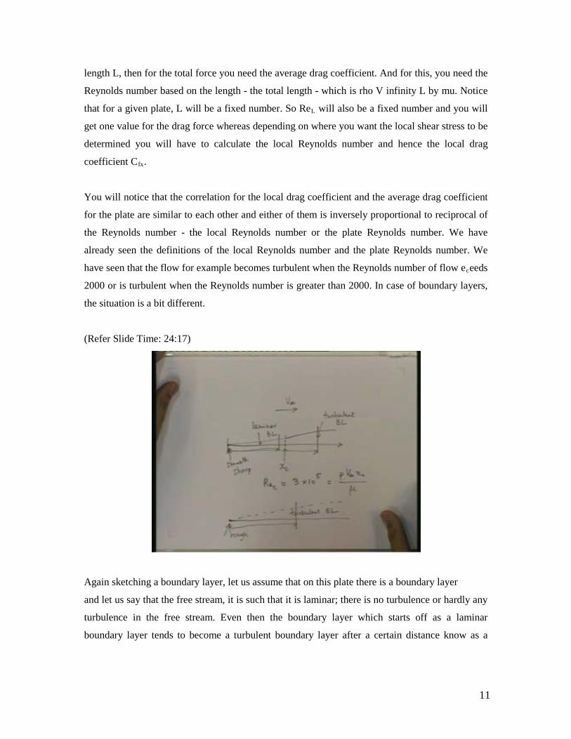
11
length L, then for the total force you need the average drag coefficient. And for this, you need the
Reynolds number based on the length - the total length - which is rho V infinity L by mu. Notice
that for a given plate, L will be a fixed number. So ReL will also be a fixed number and you will
get one value for the drag force whereas depending on where you want the local shear stress to be
determined you will have to calculate the local Reynolds number and hence the local drag
coefficient Cfx.
You will notice that the correlation for the local drag coefficient and the average drag coefficient
for the plate are similar to each other and either of them is inversely proportional to reciprocal of
the Reynolds number - the local Reynolds number or the plate Reynolds number. We have
already seen the definitions of the local Reynolds number and the plate Reynolds number. We
have seen that the flow for example becomes turbulent when the Reynolds number of flow eceeds
2000 or is turbulent when the Reynolds number is greater than 2000. In case of boundary layers,
the situation is a bit different.
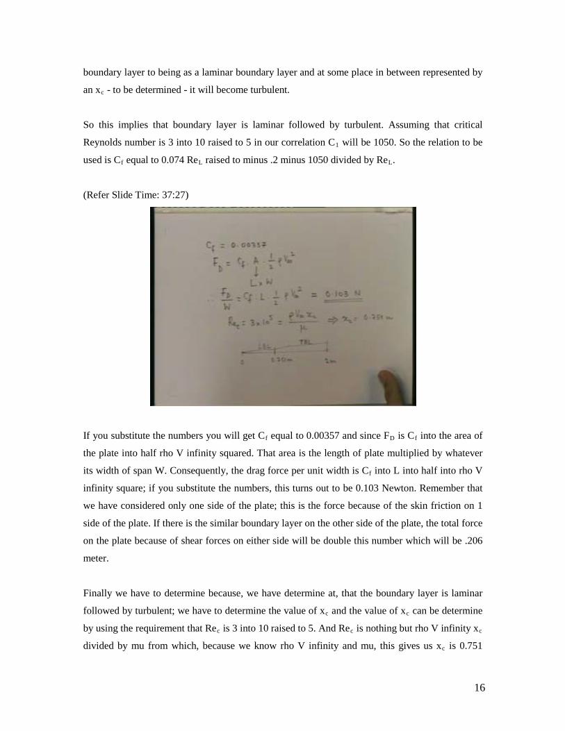
(Refer Slide Time: 24:17)
Again sketching a boundary layer, let us assume that on this plate there is a boundary layer
and let us say that the free stream, it is such that it is laminar; there is no turbulence or hardly any
turbulence in the free stream. Even then the boundary layer which starts off as a laminar
boundary layer tends to become a turbulent boundary layer after a certain distance know as a

12
transition distance and this transition distance is given by a transition or critical Reynolds number
which for flat plate is 3 into 10 raised to 5. This will be rho V infinity xc by mu.
So even though the free stream is laminar, the boundary layer may start off as a laminar boundary
layer and then may become a turbulent boundary layer. This transition to turbulence is important
and such a situation will arise only if the leading edge of the plate, it is smooth and sharp; if now
make the leading edge rough, jagged then it is possible to have a turbulent boundary layer right
from the leading edge. That is the difference between the tube situation and the boundary layer
situation; in a boundary layer situation under the same condition of a fixed V infinity, it is
possible to have a laminar boundary layer first followed by a turbulent boundary layer. Not only
that, by appropriately roughening the leading edge or putting a small extension there, you can
make the boundary layer turbulent right from the leading edge.
For the laminar part of the boundary layer, we have these analytical solutions but when the
laminar boundary layer becomes turbulent or for some reason we have a turbulent boundary
layer, we cannot obtain an analytical solution. Experimental data indicates that whenever the flow
is turbulent, the local Reynolds number is given by an expression similar to the expression for the
laminar drag coefficient.
(Refer Slide Time: 27:37)

13
This is the local drag coefficient; I have used the subscript turb indicating that it is for turbulent
boundary layer and here you will notice that it is inversely proportional to Reynolds number
raised to .2, the local Reynolds number raised to .2. This is a correlation based on a large amount
of experimental data. We have seen that it is possible to have a boundary layer which is partly
laminar and then becomes turbulent so if we have a plate in which the whole boundary layer is
laminar, we have one situation but we can also have a situation where the plate is long enough
such that the boundary layer is partly laminar partly turbulent and we could also have a situation
plate with a rough leading edge where the whole length of the plate is exposed to a turbulent
boundary layer.
We have to be careful while calculating the overall or the average drag coefficient in these
situations. If it is purely laminar, we should integrate the laminar correlation; if it is purely
turbulent, we should use the turbulent correlation for Cfx and integrate it. If it is a combination of
the two, we should appropriately take account of the laminar part and the turbulent part.
(Refer Slide Time: 29:30)
Suppose we have the possibility of the boundary layer being partly laminar and partly turbulent
then the averaging to obtain, the average drag coefficient will have to be done over part of the
boundary layer which is laminar using the laminar skin friction equation and part of the
integration to be done over the turbulent part of the boundary layer using the Cfx term which is
the turbulent boundary layer skin friction coefficient.

14
Assuming that xc is less than L that means we have partly laminar and partly turbulent boundary
layer. We get after these integrations - Cf equal to .074 ReL raised to minus .2 minus C1 divided
by ReL where C1 is 0 if the boundary layer is turbulent from the leading edge; that means there is
no effect of the laminar boundary layer. This is the effect of the laminar boundary layer and if the
transition takes place at Rec is 3 into 10 raised to 5 which is an appropriate value then the value of
C1 is 1050. Of course if we have boundary layer which is fully laminar then we should go back to
our laminar flow equation and use this correlation.
So if we are sure that the boundary layer is fully laminar we should use this equation. If the
boundary layer is partly laminar and partly turbulent we should use this equation with the value of
C1 say 1050. If the boundary layer is fully turbulent right from the leading edge then the C1 is 0
so the correlation reduces to only this part. Let us take an illustrative example.
(Refer Slide Time: 31:47)
We are considering a plate; I will show first a 3 dimensional figure, this is the leading edge of the
plate, this is the trailing edge of the plate. It is exposed to a fluid; the free stream velocity V
infinity is 4 meters per second and the fluid is air at a temperature of 20 degree c but at a pressure
of 1.5 atmosphere. In the direction of flow, the length of the plate is 2 meters; the width of the
plate is some w but it is so wide that we don’t have to worry about what happens this edge of the
plate and this edge of the plate.

15
What happens at one location is assumed to happen at another location in the width direction. We
have to determine what is the average drag coefficient, we have to determine the drag force per
unit width or per unit span, we have to determine what type of boundary layer we have assuming
a sharp leading edge sharp and smooth, and if there is a transition to turbulence, what is the
location where the transition takes place?
(Refer Slide Time: 33:54)
Let us now sketch it neatly. I am looking along the span of the plate so the width of the plate L is
2 meters. They may be a boundary layer; let us look at only side of the plate. The free stream V
infinity is 4 meters per second; we measure x from here and what flows is air at 20 degree C in 1
.5 atmosphere. At this temperature and pressure if we take properties of air - read them off from
tabulation, of course the tabulation will be at visually at atmospheric pressure so you have to note
that the density will increase as the pressure increases that the dynamic viscosity is essentially
independent of pressure. So you get mu equal to 18.1 into 10 raised to minus 6 pascal second and
the density is 1.808 kg per meter cube.
We first calculate ReL - this is rho V infinity L divided by mu. This is 1.808 into 4 into 2 divided
by 18.1 into 10 raised to minus 6 and this turns out to be 7.989 into 10 to the 5. Notice that this is
greater than 3 into 10 to the 5. Since out leading edge is smooth and sharp, we expect the
16
boundary layer to being as a laminar boundary layer and at some place in between represented by
an xc - to be determined - it will become turbulent.
So this implies that boundary layer is laminar followed by turbulent. Assuming that critical
Reynolds number is 3 into 10 raised to 5 in our correlation C1 will be 1050. So the relation to be
used is Cf equal to 0.074 ReL raised to minus .2 minus 1050 divided by ReL.
(Refer Slide Time: 37:27)
If you substitute the numbers you will get Cf equal to 0.00357 and since FD is Cf into the area of
the plate into half rho V infinity squared. That area is the length of plate multiplied by whatever
its width of span W. Consequently, the drag force per unit width is Cf into L into half into rho V
infinity square; if you substitute the numbers, this turns out to be 0.103 Newton. Remember that
we have considered only one side of the plate; this is the force because of the skin friction on 1
side of the plate. If there is the similar boundary layer on the other side of the plate, the total force
on the plate because of shear forces on either side will be double this number which will be .206
meter.
Finally we have to determine because, we have determine at, that the boundary layer is laminar
followed by turbulent; we have to determine the value of xc and the value of xc can be determine
by using the requirement that Rec is 3 into 10 raised to 5. And Rec is nothing but rho V infinity xc
divided by mu from which, because we know rho V infinity and mu, this gives us xc is 0.751

17
meters. That means if this is the plate, a total distance of 2 meters from the leading edge up to .75
meters, the boundary layer is laminar and beyond that the boundary layer is turbulent. So this is
laminar boundary layer and this is turbulent boundary layer.
After studying the flat plate which is a basic situation analytically solvable for laminar flow we
go to the other common situation which is a cylinder in cross flow, a tube in cross flow - a basic
situation in external flow important from fluid flow, important even from heat transfer; studied
extensively but rather difficult to study analytically.
(Refer Slide Time: 40:58)
If you take a cylinder and expose it to a stream flowing and the free stream velocity V infinity,
depending on the Reynolds number we get different and very complex flow situations. For a very
very low Reynolds number there is hardly any boundary layer which develops the flow, comes,
creeps around the cylinder and leaves. As you go to higher values of Reynolds number where a
nice boundary layer which develops laminar boundary layer which separates, we have a
separation zone, small separation zone that there are 2 eddies counter rotating.
At still higher Reynolds number the boundary layer separates and may also become turbulent;
sometimes the boundary layer becomes turbulent after separation, sometimes it becomes turbulent
before separation. So you may have a laminar boundary layer separating and then becoming
turbulent or a laminar boundary layer first becoming turbulent and then separating. When the

18
flow separates and these eddies form that particular path beyond the separation point is not really
a boundary layer.
A very interesting situation occurs at higher Reynolds number; there even the separated eddies -
they don’t remain attached to the cylinder. We have one eddy being discharged or disengaging
from the cylinder, another eddy a third eddy and so on. Alternatively an eddy will form on one
side angle separate from the cylinder, another eddy will form on the other side and separate from
the cylinder and so on. This is what is known as the Von Karmen vortex street which occurs at a
reasonably large Reynolds number and this is a very interesting and complicated flow situation
where you have some sort of a periodic shedding of eddies.
In fact because of this alternate shedding, a lift force which oscillates in the cross-stream direction
perpendicular to the approaching free stream velocity now acts on the cylinder and if the cylinder
is flexible say a long wire hanging, it will start oscillating and sometimes you get a nice musical
note out of this - a whistling type of note because this frequency happens to be in the frequencies
which we can hear. Each one of these different situations lead to different drag coefficients
and the drag coefficient here CD, D because it is based on the diameter, is defined as the drag
force which is force in the direction of the approaching velocity divided by area divided by rho V
V infinity squared by 2.
Once you remember here that unlike the flat plate where we took the plate area, this area is the
projected area. Area projected in the direction of flow so the area will be not pi D into the length
of the cylinder but basically be D into the length of the cylinder. That is something which we
should remember because of the variation in the flow pattern at different Reynolds number. The
situation is very complicated for analysis and except perhaps for very low Reynolds number,
situations like these cannot be analytically handled at all.

19
(Refer Slide Time: 46:17)
So we have semi analytical and experimental correlations for CD as a function of Reynolds
number and here we have the correlation which is valid from a Reynolds number as well as .1;
below .1 the flow situation will be something like this. And as the Reynolds number increases, it
moves to something like this to like this to like this and as the flow situation changes, the
correlations change. First you will notice that CD is inversely proportional to roughly two-thirds
power of Reynolds number. Then in another range of Reynolds number CD is proportional to
roughly the fourth root of Reynolds number inversely proportional, then over a small range of
Reynolds number from 1000 to 5000, it remains more or less constant at 1. Beyond that the CD
increases with Reynolds number, roughly Reynolds number to the power 1-8 or so and beyond
that from 10 raised to 4 to 2 into 10 raised 5 can be approximated to a constant value of 1.1. All
these different things occur because of the different flow situations that we have analyzed or
looked at so far. Let us now take an illustrative example of flow across a cylinder.

20
(Refer Slide Time: 47:52)
Here we have a cylinder; the diameter of the cylinder is 75 millimeters. Air flows across the
cylinder 60 degree C, one atmosphere. The approaching velocity is 2 meters per second; cylinder
is long at some length L. Naturally a drag coefficient acts on the cylinder, drag force acts on the
cylinder. We have to determine the drag coefficient and then determine the drag force per unit
length of the cylinder.
We start off by obtaining the properties of air at 60 degree C and 1 atmosphere. We will need
density and we will need viscosity - any one of the two viscosities will do. The density turns out
to be 1.060 kilogram per meter cube; kinematic viscosity is 18.97 into 10 raised to minus 6
meters squared per second. We first calculate the Reynolds number based on the diameter; this
will be V infinity D divided by kinematic viscosity mu - this will be 2.0 diameter 0.075 meter
kinematic viscosity 18.97 10 raised to minus 6 this turns out to be 7907. So going back to our
correlations, we find ourselves in this range 5000 to 10000; ours is something near 8000 and
hence this is the correlation which is to be used for the drag force.
So CD turns out to be 0.310 ReD raised to .1375; substituting the values we get this as 1.065. At
high Reynolds number CD will be roughly equal to 1, between 1 and 1.1. The drag force is CD
into projected area which will be D into L multiplied by rho V infinity squared by 2 and hence the
drag force per unit length of the cylinder will be CD into D into rho V infinity squared by 2 and if

21
you substitute these numbers you will get this to be 0.169 Newton per meter. So if it is a ten-
meter long cable this will be about 1.7 Newtons.
This particular illustration shows how to calculate the drag coefficient. In particular remember
that for cylinders and you will have correlations for a square body or a sphere. These correlations
are available in textbooks and in literature. Whenever we have a body, expect a thin plate which
has a significant projected area to the flow; it is the projected area which is used for determining
the drag force. It is only for a thin flat plate that we use the actual area of the plate. Now in these
2 lectures we have briefly reviewed fluid mechanics.
(Refer Slide Time: 53:50)
This was only a review of fluid mechanics because it is needed for a study of convection in which
fluid flow and heat transfer go together. We looked at the governing equations, then we looked at
internal flows and then we looked at external flows. We solved some illustrative example to
determine the pressure drop and the drag force. With this review of fluid mechanics we are now
ready to begin the study of convection. We begin with a study of force convection in the next
lecture.