Heavy-Traffic Extreme-Value Limits for Erlang Delay Models

Guodong Pang and Ward Whitt

IEOR DepartmentColumbia University

{gp2224,ww2040}@columbia.edu

March 16, 2009

Abstract

We consider the maximum queue length and the maximum number of idle servers in the classical

Erlang delay model and the generalization allowing customer abandonment – the M/M/n + M

queue. We use strong approximations to show, under regularity conditions, that properly scaled

versions of the maximum queue length and maximum number of idle servers over subintervals in

the delay models converge jointly to independent random variables with the Gumbel extreme-value

distribution in the QED and ED many-server heavy-traffic limiting regimes as n and t increase to

infinity together appropriately; we require that tn → ∞ and tn = o(n1/2−ε) as n → ∞ for some

ε > 0 .

Keywords: Erlang models, many-server queues, extreme values, heavy traffic, diffusion approx-

imations, strong approximations, limit theorems.

1 Introduction

It is remarkable how persistently the multiserver Erlang B (loss) and C (delay) models have re-

mained the workhorse models for performance analysis of multiserver systems, ever since A. K.

Erlang introduced them one hundred years ago. Over the years, the original applications to

telecommunication systems have continued, while new applications have emerged, e.g., to new

communication systems, call centers, hospitals and other service systems; e.g., see Gans et al.

(2003) for a survey on call-centers.

In this paper, we will once again consider the basic Erlang delay model as well as the so-called

Erlang A or Palm (M/M/n+M) model, which includes customer abandonment. The Erlang B and

C models appear as the special cases in which the abandonment rate is infinite and zero, respectively.

1

We will be concerned with asymptotic results that facilitate extreme-value engineering; see Castillo

(1988). The idea is to judge whether staffing is appropriate, neither inadequate nor excessive, by

looking at the maximum queue length and the maximum number of idle servers over specified time

intervals, such as a single hour. Our goal is to apply extreme-value theory, as in Embrechts et al.

(1997), to develop a systematic way to interpret such extreme-value measurements.

However, there are two difficulties, which motivate this research. The first difficulty is discrete-

ness. It is well known that the classical extreme-value theory does not apply to integer-valued

random variables. For example, with an infinite-server M/M/∞ queue, the steady-state distribu-

tion of the number of customers in the system is Poisson, and the maximum of i.i.d. (or weakly

dependent) Poisson random variables does not have a nondegenerate extreme-value limit; see Ex-

ample 1.7.14 in Leadbetter et al. (1982). Another example is the M/M/n/∞ queue, which has a

steady-state distribution with a geometric upper tail; see Theorem 1.3 of Serfozo (1988).

The second difficulty is the common occurrence of time-varying arrival rates in service systems.

The demand typically varies greatly by time of day. In response, the staffing levels typically vary

by time of day as well. Since the service times are often short and the arrival rate tends to change

relatively slowly, it is often appropriate to use time-varying steady-state performance measures,

the so-called pointwise stationary approximation reviewed in Green et al. (2007). Indeed, we will

assume that the subintervals over which we consider extreme values are short enough that the

queueing processes can be regarded as approximately stationary; the intervals might be one hour

long. However, different hours at different times of the day might have very different arrival rates.

We want a systematic way to relate the extreme values over different hours with very different

arrival rates (and staffing). We also want to combine measurements from different hours that may

have very different arrival rates. There is a problem, because even with proper staffing set to achieve

target service-level constraints throughout the day, the distributions of the maximum queue length

and the maximum number of idle servers depend on the arrival rate and the staffing level n. We

would like performance measures that are easy to interpret directly, without having to relate to the

staffing level.

We propose addressing both difficulties for extreme values by applying extreme-value approx-

imations (obtained as t → ∞) associated with diffusion approximations (obtained as n → ∞). A

key ingredient is appropriate scaling. The diffusion approximations follow from the many-server

heavy-traffic limits (as n → ∞) established by Halfin and Whitt (1981), Garnett et al. (2002)

and Whitt (2004). In this limit, properly scaled queueing processes converge to diffusion processes,

2

which have continuous steady-state distributions. In particular, we can then apply extreme-value

limits for diffusion processes (as t → ∞) established by Davis (1982), Borkovec and Kluppelberg

(1998) and references therein. The scaling in the many-server heavy-traffic limits also allows us

to address the difficulty posed by time-varying demand. With the proper scaling, the resulting

approximation can be interpreted independent of the staffing level n, provided that the queueing

processes can be considered approximately stationary for each n.

The procedure we have described involves an iterated limit in which we first let n → ∞, and

then afterwards let t → ∞. However, in an application we have fixed n and t. We have already

observed that we cannot reverse the order of the limits. In order to obtain good approximations

for fixed n and t, here we consider the double limit in which n → ∞ and t → ∞ jointly; i.e., we

let tn →∞ as n→∞, imposing a regularity condition that tn not increase too rapidly, in order to

avoid the discreteness problem. After scaling, the resulting approximation will be independent of

n and t.

Our general approach for obtaining double limits for many-server queues follows the procedure

used by Glynn and Whitt (1995) to treat single-server queues. As they did, we exploit strong

approximations. However, Glynn and Whitt (1995) used strong approximations for partial sums

by Brownian motion, as in Csorgo and Revesz (1981). Since the stochastic process representing the

number in system for the M/M/n+M model can be represented in terms of random-time changed

Poisson processes, here we will apply strong approximations for Poisson processes by Brownian

motion, as in Kurtz (1978). We also apply the main result from Glynn and Whitt (1995) as an

intermediate step in our proof; see Lemma 3.2.

Even though standard extreme-value limits are difficult for the integer-valued queue-length

process, there is some relevant literature. Sadowsky and Szpankowski (1995) and references therein

describe various bounds on the distribution of the maximum queue length for GI/G/c queues.

Algorithms have been proposed to compute the distribution of the maximum queue length in

a busy period for M/M/c retrial queues for application to call-center management by Artalejo

(2007) and Artalejo et al. (2007). Serfozo (1988) and McCormick and Park (1992) have obtained

extreme-value limits for the maximum queue length of M/M/c queues by allowing the birth rates

and death rates to vary in a certain manner as the time interval increases. Asmussen (1998) has

given a good survey on the cycle maxima approach for extreme value limits in queues. Evidently,

nobody has previously done the natural thing we do here.

This paper is organized as follows: In §2, we introduce the scaled processes and state the

3

convergence results. In §3 we give proofs. We give all details for the proof of Theorem 2.2 and

sketch the remaining proofs, which are similar.

2 The Convergence Results

We consider a sequence of M/M/n+M queueing models (with unlimited waiting space) indexed by

the number of servers n and let n ↑ ∞. The arrival process is Poisson with rate λn, service times are

i.i.d. with an exponential distribution having mean µ−1 and customers abandon independently with

an exponential distribution having mean θ−1. For each n, we assume that the arrival process, service

times and abandonment times are mutually independent. The traffic intensity is ρn ≡ λn/nµ.

Assume that λn/n→ λ ∈ (0,∞) as n→∞.

We use the conventional notation: x ∧ y ≡ min{x, y}, x ∨ y ≡ max{x, y}, x+ ≡ max{x, 0} and

x− ≡ max{−x, 0} for x, y ∈ R; log is always the natural logarithm (base e); Dk ≡ D([0,∞),Rk) is

the space of right-continuous functions with left limits in Rk, with Dk ≡ D for k = 1; ⇒ denotes

convergence in distribution; see Billingsley (1999) and Whitt (2002) for background.

2.1 The Processes of Interest

For each n ≥ 1 and t ≥ 0, let Xn(t), Qn(t) ≡ (Xn(t)− n)+ and In(t) ≡ (Xn(t)− n)− represent the

number of customers in the system, the queue length, and the number of idle servers, respectively.

Let Xn ≡ {Xn(t) : t ≥ 0}, Qn ≡ {Qn(t) : t ≥ 0} and In ≡ {In(t) : t ≥ 0} be the associated

stochastic processes. Assume that the initial condition Xn(0) is independent of the arrival, service

and abandonment processes.

Under those assumptions, the process Xn can be represented as

Xn(t) = Xn(0) +A(λnt)− S(∫ t

0µ(Xn(s) ∧ n)ds

)− L

(∫ t

0θ(Xn(s)− n)+ds

), t ≥ 0, (2.1)

where A ≡ {A(t) : t ≥ 0}, S ≡ {S(t) : t ≥ 0} and L ≡ {L(t) : t ≥ 0} are mutually independent

Poisson processes with unit rate.

Define the running maximum and minimum processes of Xn, Mn ≡ {Mn(t) : t ≥ 0} and

Nn ≡ {Nn(t) : t ≥ 0}, respectively, by

Mn(t) ≡ max0≤s≤t

Xn(s), Nn(t) ≡ min0≤s≤t

Xn(s), t ≥ 0. (2.2)

Define processes MQn ≡ {MQ

n (t) : t ≥ 0} and M In ≡ {M I

n(t) : t ≥ 0} representing the maximum

4

queue length and the maximum number of idle servers by

MQn (t) ≡ max

0≤s≤tQn(s) = (Mn(t)− n)+, M I

n(t) ≡ max0≤s≤t

In(s) = (n−Nn(t))+, t ≥ 0. (2.3)

We are interested in the asymptotic behavior of Mn, Nn, MQn and M I

n as n → ∞ and t → ∞

simultaneously. In the next two subsections, we will state the extreme-value limit theorems for

these processes in the QED and ED regimes. In subsequent subsections we will consider other

variants of the M/M/n+M model: the Erlang C model and the infinite-server queue.

2.2 Erlang A: QED

With customer abandonment (0 < θ < ∞), in the QED regime the system is asymptotically

critically loaded; i.e., we assume that

√n(1− ρn)→ β, as n→∞, β ∈ R. (2.4)

The scaling in (2.4) is consistent with the classical square-root-staffing principle for large n, provided

that β > 0. However, abandonment makes it possible to have β ≤ 0 as well. By assuming (2.4),

we are assuming that the system is staffed properly, where the parameter β determines the quality

of service more precisely.

Define the scaled processes Xn ≡ {Xn(t) : t ≥ 0}, Xn ≡ {Xn(t) : t ≥ 0}, Mn ≡ {Mn(t) : t ≥ 0},

MQn ≡ {MQ

n (t) : t ≥ 0}, M In ≡ {M I

n(t) : t ≥ 0}, and Nn ≡ {Nn(t) : t ≥ 0}, where

Xn(t) ≡ Xn(t)n

, Xn(t) ≡ Xn(t)− n√n

, Mn(t) ≡ Mn(t)− n√n

, Nn(t) ≡ Nn(t)− n√n

,

MQn (t) ≡ MQ

n (t)√n

= Mn(t)+, M In(t) ≡ M I

n(t)√n

= (−Nn(t))+, t ≥ 0. (2.5)

It was proved in Garnett et al. (2002) that, if there exists a random variable X(0) such that

Xn(0) ⇒ X(0) in R as n → ∞, then Xn ⇒ X in D as n → ∞, where the limit X is the diffusion

process with infinitesimal mean ν(x) = −βµ − θx for x ≥ 0 and ν(x) = −βµ − µx for x < 0, and

infinitesimal variance σ2(x) = 2µ, i.e.,

X(t) = X(0)− βµt−∫ t

0µ(X(s) ∧ 0)ds−

∫ t

0θ(X(s) ∨ 0)ds+

√2µB(t), t ≥ 0, (2.6)

where B ≡ {B(t) : t ≥ 0} is a standard Brownian motion.

Moreover, stationary distributions exist and converge; i.e., X(t)⇒ X(∞) and Xn(t)⇒ Xn(∞)

as t → ∞ for each n, and Xn(∞) ⇒ X(∞) as n → ∞. Hence, we can initialize with stationary

distributions, i.e., we can regard all the processes as stationary processes. That is not required

5

for the extreme-value limits, see Theorem 3.1, but it is realistic for applications and clearly should

make the approximations perform better for smaller sample size.

Let M ≡ {M(t) : t ≥ 0} and N ≡ {N(t) : t ≥ 0} be the running maximum and minimum

processes of X, respectively, i.e.,

M(t) ≡ max0≤s≤t

X(s) and N(t) ≡ min0≤s≤t

X(s), t ≥ 0. (2.7)

It follows immediately from applying the continuous mapping theorem (§13.4, Whitt 2002) that, if

there exists a random variable X(0) such that Xn(0)⇒ X(0) in R as n→∞, then

(Mn, Nn)⇒ (M, N) in D2 as n→∞. (2.8)

We first characterize the extremal behavior of the limit diffusion process X in (2.6) in the

following proposition. We apply the general extreme-value limit theorems established in Davis

(1982) and Borkovec and Kluppelberg (1998), which are summarized in §3.1. The proof is given

in §3.2. The extreme-value limits for the maximum process M and the minimum process N are

asymptotically independent as t → ∞; see Theorem 3.4 in Davis (1982). In all our extreme-value

limits, the limiting random variables will have the standard Gumbel distribution; let Z denote such

a random variable; i.e., P (Z ≤ x) ≡ e−e−x, x ∈ R. The general form of the scaling we obtain in our

heavy-traffic extreme-value limits combines the heavy-traffic scaling with the extreme-value scaling.

The extreme-value scaling is similar to the scaling for the maximum of i.i.d. random variables with

the steady-state distribution of the diffusions process, but there are minor differences. In general,

extreme-value limits for recurrent diffusion processes are not characterized by their steady-state

distributions; see §3.1.

Proposition 2.1 The extremal processes M and N of the limit diffusion process X defined in (2.6)

and (2.7) have the joint limit:(M(t)− b(t)

a(t),−N(t)− d(t)

c(t)

)⇒ (Z1, Z2) in R2 as t→∞, (2.9)

where Z1 and Z2 are independent random variables with the standard Gumbel distribution, and

a(t) ≡ r/√

2 log t, c(t) ≡ 1/√

2 log t,

b(t) ≡ r√

2 log t− βr2 +r√

8 log t

(log log t+ log(θ2α2π−1(1− Φ(rβ))−2)

),

d(t) ≡√

2 log t− β +(

log log t+ log(µ2(1− α)2π−1Φ(β)−2)√8 log t

),

α ≡(

1 +φ (rβ) Φ(β)

r(1− Φ (rβ))φ(β)

)−1

, r ≡√µ/θ, (2.10)

6

where Φ and φ are the cdf and pdf of the standard normal distribution.

Notice that a(t) → 0, as t → ∞, so that we have the limit M(t) − b(t) ⇒ 0 as t → ∞ as a

consequence of Proposition 2.1; i.e., there is a concentration about b(t) without additional scaling,

and similarly for the other processes. By first letting n → ∞ and then letting t → ∞, we obtain

the following extreme-value limit theorem for the extremal processes Mn, Nn, MQn and M I

n.

Theorem 2.1 Consider the M/M/m/∞+M queueing model in the QED regime specified in (2.4).

If there exists a random variable X(0) such that Xn(0)⇒ X(0) in R as n→∞, then(Mn(t)− b(t)

a(t),MQn (t)− b(t)a(t)

,−Nn(t)− d(t)

c(t),M In(t)− d(t)c(t)

)⇒ (Z1, Z1, Z2, Z2) in R4 (2.11)

as first n → ∞ and then t → ∞, where Z1 and Z2 are independent with the standard Gumbel

distribution and a(t), b(t), c(t) and d(t) are as given in (2.10).

We next establish an extreme-value limit as n→∞ and t→∞ simultaneously by imposing a

condition that tn not increase too rapidly.

Theorem 2.2 If, in addition to the assumptions of Theorem 2.1, tn → ∞ and tn/n1/2−ε → 0 as

n→∞ for some ε > 0, then(Mn(tn)− bn(tn)

an(tn),MQn (tn)− bn(tn)an(tn)

,−Nn(tn)− dn(tn)

cn(tn),M In(tn)− dn(tn)cn(tn)

)⇒ (Z1, Z1, Z2, Z2),

(2.12)

in R4 as n→∞, where Z1 and Z2 are independent with the standard Gumbel distribution,

an(tn) ≡ rγn√2 log tn

, cn(tn) =γn√

2 log tnbn(tn) ≡ rγn

√2 log tn − βnr2

+rγn√

8 log tn

(log log tn + log

(θ2α2

nπ−1 (1− Φ(βnr/γn))−2

)),

dn(tn) ≡ γn√

2 log tn − βn

+γn√

8 log tn

(log log tn + log

(θ2(1− α2

n)π−1 (1− Φ(βn/γn))−2))

,

αn ≡(

1 +φ(βnr/γn))

r(1− Φ(βnr/γn))

(Φ(βn/γn)φ(βn/γn)

))−1

→ α,

βn ≡√n(1− ρn)→ β and γn ≡

√[(λn/n) + µ]/2µ→ 1 as n→∞, (2.13)

for β in (2.5) and α and r in (2.10). Moreover, the constants an(tn), bn(tn), cn(tn), and dn(tn)

can be replaced by a(tn), b(tn), c(tn), and d(tn), respectively, which are defined in (2.10).

7

We conjecture that the heavy-traffic extreme-value limit for the process M In in the Erlang B

model is given in Theorem 2.2, where we let θ → ∞ in the normalization constants. Note that θ

does not appear in cn and only affects dn through αn, which only appears in the lowest-order term.

The M/M/n+M model provides a lower bound.

Based on Theorem 2.2, we can approximate the random vector (MQn (t),M I

n(t)) without scaling

in the usual way by

(MQn (t),M I

n(t)) ≈ (√n[an(t)Z1 + bn(t)],

√n[cn(t)Z2 + dn(t)])

for large t, where the constants an(t), bn(t), cn(t) and dn(t) are given in (2.13), and (Z1, Z2) is a

pair of independent random variables, each with the Gumbel distribution. Since E[Z] ≈ 0.57721,

the Euler-Mascheroni constant, and V ar(Z) = π2/6, we obtain simple explicit approximations for

the mean and variance of the extremal variables MQn (t) and M I

n(t) for large t, e.g.,

E[MQn (t)] ≈

√n(0.577an(t) + bn(t)), V ar(MQ

n (t)) ≈ na2n(t)π2/6.

Moreover, we can also approximate the spread of Xn, i.e., SXn (t) ≡Mn−Nn = MQn (t) +M I

n(t), by

SXn (t) ≈√n(bn(t) + dn(t) + an(t)Z1 + cn(t)Z2)

for large t.

However, for applications we suggest applying the approximation with the scaling. Over different

hours, the scaled maximum random variables in (2.12) all approximately have the standard Gumbel

distribution independent of n, provided that n is not too small. With the scaling, the maximum

of k maxima over several separate hours can be approximated as the maximum of k i.i.d. random

variables, each with the standard Gumbel distribution, which is again a (non-standard) Gumbel

distribution. If we want, we can apply yet another extreme-value limit as k →∞, which yields the

standard Gumbel distribution with proper scaling.

2.3 Erlang A: ED

In the ED regime, the system is overloaded; i.e., we assume that λn = nλ and λ > µ. It is

proved in Whitt (2004) that the fluid scaled process XEDn ≡ Xn/n converges to the constant limit

XED(t) ≡ 1 + (λ − µ)/θ in D as n → ∞ if the scaled initial values converge: XEDn (0) ⇒ XED(0)

as n→∞. Define the diffusion scaled processes XEDn ≡ {XED

n (t) : t ≥ 0}, and the scaled extremal

8

processes MEDn ≡ {MED

n (t) : t ≥ 0} and MQ,EDn ≡ {MQ,ED

n (t) : t ≥ 0} by

XEDn (t) ≡ XED

n (t)− n(1 + (λ− µ)/θ)√n

, and MEDn (t) ≡ Mn(t)− n(1 + (λ− µ)/θ)√

n,

MQ,EDn (t) ≡ MQ

n (t)− n(λ− µ)/θ√n

, t ≥ 0. (2.14)

It is also proved in Whitt (2004) that if, in addition, XEDn (0)⇒ XED(0) as n→∞, then XED

n ⇒

XED in D as n→∞, where the limit process XED ≡ {XED(t) : t ≥ 0} is an OU process, given by

XED(t) = XED(0) +√

2λB(t)− θ∫ t

0XED(s)ds, t ≥ 0, (2.15)

where B is a standard Brownian motion. As in §2.2, limiting steady-state distributions exist and

converge, so that it is natural to assume that we initialize with the steady-state distributions, so

that we have stationary processes. The extremal behavior of OU processes has been well studied;

see Proposition 3.1. Thus, we have the following extreme-value result, paralleling Theorems 2.1

and 2.2.

Theorem 2.3 Consider the M/M/n/∞ + M queueing model in the ED regime. If XEDn (0) ⇒

XED(0) in R as n→∞, then(MEDn (t)− b(t)

a(t),MQ,EDn (t)− b(t)

a(t)

)⇒ (Z,Z) in R2, (2.16)

either (i) as first n→∞ and then t→∞ with

a(t) ≡

√λ

2θ log t, b(t) ≡

√2λ log tθ

+

√λ

8θ log t(log log t+ log(θ2/π)

). (2.17)

or (ii) if in addition t is replaced by tn, where tn → ∞ and tn/n1/2−ε → 0 as n → ∞ for some

ε > 0.

2.4 Erlang C: QED

The story changes if we have no customer abandonment (θ = 0). Without abandonment, the QED

regime is again defined by (2.4) but with β > 0. The representation of the process Xn in (2.1)

becomes

Xn(t) = Xn(0) +A(λnt)− S(∫ t

0µ(Xn(s) ∧ n)ds

), t ≥ 0, (2.18)

where A = {A(t) : t ≥ 0} and S = {S(t) : t ≥ 0} are independent unit-rate Poisson processes.

Thus the limit diffusion process X in (2.6) becomes

X(t) = X(0)− βµt−∫ t

0µ(X(s) ∧ 0)ds+

√2µB(t), t ≥ 0, (2.19)

9

where B ≡ {B(t) : t ≥ 0} is a standard Brownian motion. Halfin and Whitt (1981) showed that the

steady-state distribution is a combination of a normal pdf below 0 and an exponential pdf above

0; see (3.13) and Browne and Whitt (1995) for an explanation.

Paralleling Proposition 2.1, we have the following characterization of the extremal behavior of

the limit process X in (2.19).

Proposition 2.2 The scaled versions of the extremal processes M and N of the limit diffusion

process X defined in (2.19) converge jointly:(M(t)− b(t)

a(t),−N(t)− d(t)

c(t)

)⇒ (Z1, Z2) in R2 as t→∞, (2.20)

where Z1 and Z2 are independent with the standard Gumbel distribution, a(t) ≡ 1/β, b(t) ≡ (log t+

log(β2µα))/β, c(t) and d(t) are the same as in (2.10), with α replaced by

α ≡ (1 + βΦ(β)/φ(β))−1 . (2.21)

Thus, paralleling Theorems 2.1 and 2.2, we obtain the following result.

Theorem 2.4 Consider the M/M/n/∞ queueing model in the QED regime. If Xn(0)⇒ X(0) in

R as n → ∞, then (2.12) holds either (i) as first n → ∞ and then t → ∞ with the normalization

constants a(t), b(t), c(t) and d(t) given in Proposition 2.2, or (ii) if in addition t is replaced by tn,

where tn →∞ and tn/n1/2−ε → 0 as n→∞ for some ε > 0, with the normalization constants

an(tn) ≡ γ2n/βn, bn(tn) ≡

[log tn + log

(µβ2

nαn/γ2n

)](γ2n/βn)

αn ≡ (1 + (βn/γn)Φ(βn/γn)/φ(βn/γn))−1 , (2.22)

cn(tn) and dn(tn) are given in (2.13) with αn replaced by αn in (2.22), and βn and γn are defined in

(2.13). Moreover, the constants an(tn), bn(tn), cn(tn), and dn(tn) can be replaced by a(tn), b(tn),

c(tn), and d(tn), which are defined in Proposition 2.2.

2.5 The Infinite-Server Model

Another important special case of the M/M/n + M model arises with parameter values θ = µ,

which is equivalent to the infinite-server M/M/∞ model. It only requires the limit theorem for

Mn. The normalization constants in Theorems 2.1 and 2.2 are simplified to

a(t) =1√

2 log t, an(tn) =

γn√2 log tn

, b(t) =√

2 log t− β +

(log log t+ log(µ2/π)

)√

8 log t,

bn(tn) = γn√

2 log tn − βn +γn(log log tn + log(µ2/π)

)√

8 log tn,

and βn and γn are defined in (2.13).

10

3 Proofs

3.1 Preliminaries: General Results for Diffusion Processes

The asymptotic behavior of the extremes of general diffusion processes has been established in

Davis (1982), Borkovec and Kluppelberg (1998) and reference therein. The following is Proposi-

tion 3.1 and Corollary 3.2 of Borkovec and Kluppelberg (1998). It is significant that, in general,

extreme-value limits for diffusion processes are not determined by the steady-state distribution of

the diffusion process, even assuming that it is well defined.

Theorem 3.1 Consider the process general diffusion process {Y (t) : t ≥ 0} in R defined by

dY (t) = ν(Y (t))dt+ σ(Y (t))dB(t), t ≥ 0, Y (0) = y,

and its running maximum process MYt ≡ max0≤s≤t Y (s). Suppose it satisfies the following condi-

tions: Y is recurrent, its speed measure m has total mass |m| <∞ and the scale function s satisfies

s(+∞) = −s(−∞) =∞. Then for any y ∈ R and any ut ↑ ∞,

limt→∞|P (MY

t ≤ ut|Y (0) = y)− F (ut)t| = 0,

where F is a distribution function, defined by

F (x) = e− 1|m|s(x) 1(z,∞)(x), x ∈ R, z ∈ R, (3.1)

with the values of s(x) and |m| depend on the choice of z. Moreover, the tail of F satisfies

F c(x) ≡ 1− F (x) ∼(|m|

∫ x

zs′(y)dy

)−1∼ (|m|s(x))−1 as x→∞.

Theorem 3.7 of Borkovec and Kluppelberg (1998) further characterizes the tail behavior of F

in Theorem 3.1 by imposing conditions on the drift coefficient ν(x) and the volatility coefficient

σ(x); we only apply part (c) of that theorem. This next result connects the cdf F in (3.1) to the

steady-state distribution of the diffusion process under further conditions.

Theorem 3.2 Under the conditions of Theorem 3.1, if ν and σ are differentiable functions on

(x0,∞) for some x0 <∞ such that

limx→∞

d

dx

(σ2(x)ν(x)

)= 0 and lim

x→∞

σ2(x)ν(x)

exp(− 2

∫ x

z

ν(t)σ2(t)

dt)

= −∞,

then F c(x) ∼ |ν(x)|h(x) as x→∞, where h is the stationary density of Y .

11

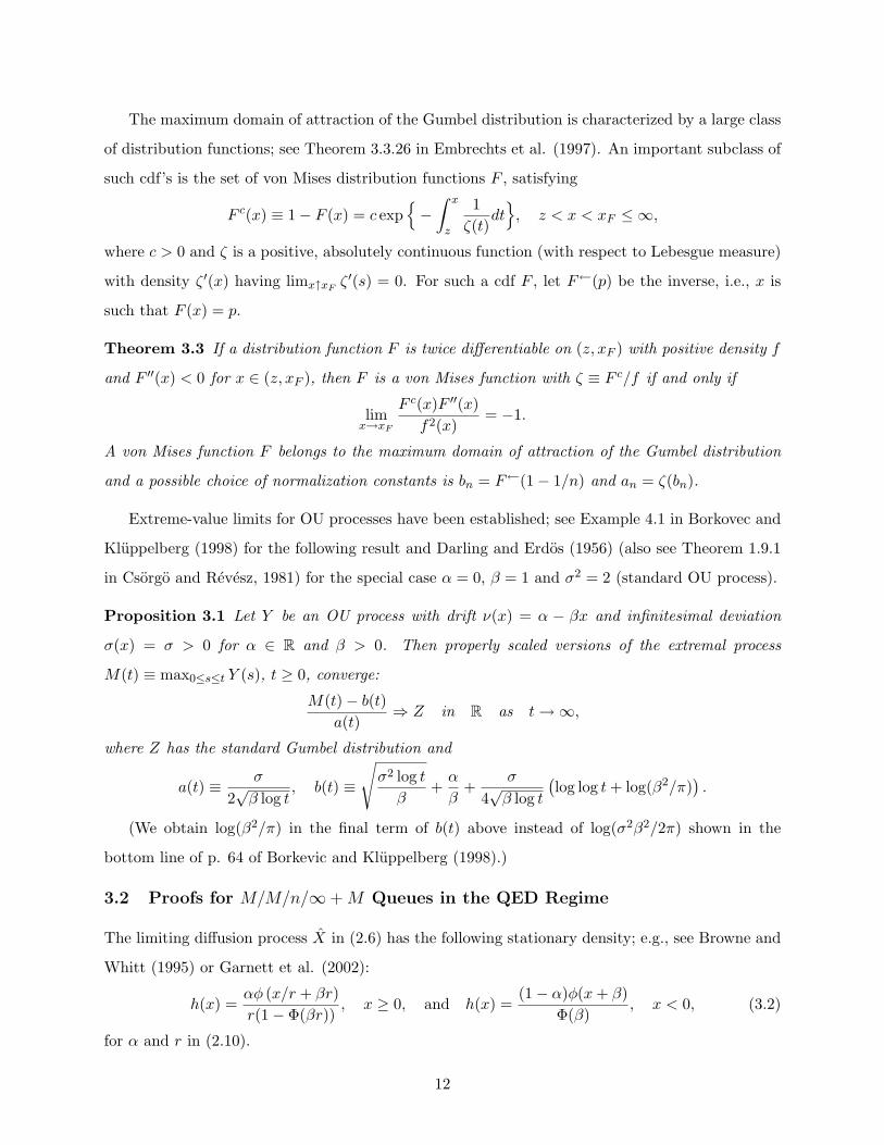
The maximum domain of attraction of the Gumbel distribution is characterized by a large class

of distribution functions; see Theorem 3.3.26 in Embrechts et al. (1997). An important subclass of

such cdf’s is the set of von Mises distribution functions F , satisfying

F c(x) ≡ 1− F (x) = c exp{−∫ x

z

1ζ(t)

dt}, z < x < xF ≤ ∞,

where c > 0 and ζ is a positive, absolutely continuous function (with respect to Lebesgue measure)

with density ζ ′(x) having limx↑xFζ ′(s) = 0. For such a cdf F , let F←(p) be the inverse, i.e., x is

such that F (x) = p.

Theorem 3.3 If a distribution function F is twice differentiable on (z, xF ) with positive density f

and F ′′(x) < 0 for x ∈ (z, xF ), then F is a von Mises function with ζ ≡ F c/f if and only if

limx→xF

F c(x)F ′′(x)f2(x)

= −1.

A von Mises function F belongs to the maximum domain of attraction of the Gumbel distribution

and a possible choice of normalization constants is bn = F←(1− 1/n) and an = ζ(bn).

Extreme-value limits for OU processes have been established; see Example 4.1 in Borkovec and

Kluppelberg (1998) for the following result and Darling and Erdos (1956) (also see Theorem 1.9.1

in Csorgo and Revesz, 1981) for the special case α = 0, β = 1 and σ2 = 2 (standard OU process).

Proposition 3.1 Let Y be an OU process with drift ν(x) = α − βx and infinitesimal deviation

σ(x) = σ > 0 for α ∈ R and β > 0. Then properly scaled versions of the extremal process

M(t) ≡ max0≤s≤t Y (s), t ≥ 0, converge:

M(t)− b(t)a(t)

⇒ Z in R as t→∞,

where Z has the standard Gumbel distribution and

a(t) ≡ σ

2√β log t

, b(t) ≡

√σ2 log tβ

+α

β+

σ

4√β log t

(log log t+ log(β2/π)

).

(We obtain log(β2/π) in the final term of b(t) above instead of log(σ2β2/2π) shown in the

bottom line of p. 64 of Borkevic and Kluppelberg (1998).)

3.2 Proofs for M/M/n/∞+ M Queues in the QED Regime

The limiting diffusion process X in (2.6) has the following stationary density; e.g., see Browne and

Whitt (1995) or Garnett et al. (2002):

h(x) =αφ (x/r + βr)r(1− Φ(βr))

, x ≥ 0, and h(x) =(1− α)φ(x+ β)

Φ(β), x < 0, (3.2)

for α and r in (2.10).

12

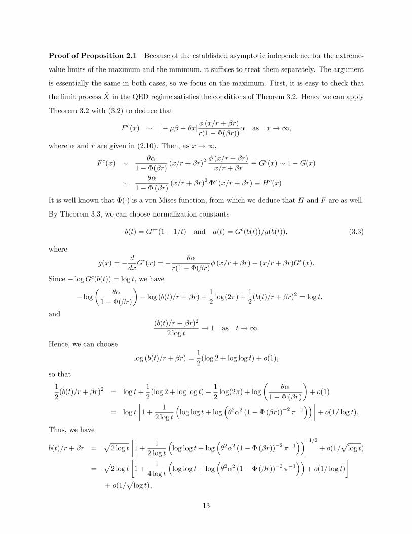
Proof of Proposition 2.1 Because of the established asymptotic independence for the extreme-

value limits of the maximum and the minimum, it suffices to treat them separately. The argument

is essentially the same in both cases, so we focus on the maximum. First, it is easy to check that

the limit process X in the QED regime satisfies the conditions of Theorem 3.2. Hence we can apply

Theorem 3.2 with (3.2) to deduce that

F c(x) ∼ | − µβ − θx| φ (x/r + βr)r(1− Φ(βr))

α as x→∞,

where α and r are given in (2.10). Then, as x→∞,

F c(x) ∼ θα

1− Φ(βr)(x/r + βr)2

φ (x/r + βr)x/r + βr

≡ Gc(x) ∼ 1−G(x)

∼ θα

1− Φ (βr)(x/r + βr)2 Φc (x/r + βr) ≡ Hc(x)

It is well known that Φ(·) is a von Mises function, from which we deduce that H and F are as well.

By Theorem 3.3, we can choose normalization constants

b(t) = G←(1− 1/t) and a(t) = Gc(b(t))/g(b(t)), (3.3)

where

g(x) = − d

dxGc(x) = − θα

r(1− Φ(βr)φ (x/r + βr) + (x/r + βr)Gc(x).

Since − logGc(b(t)) = log t, we have

− log(

θα

1− Φ(βr)

)− log (b(t)/r + βr) +

12

log(2π) +12

(b(t)/r + βr)2 = log t,

and(b(t)/r + βr)2

2 log t→ 1 as t→∞.

Hence, we can choose

log (b(t)/r + βr) =12

(log 2 + log log t) + o(1),

so that

12

(b(t)/r + βr)2 = log t+12

(log 2 + log log t)− 12

log(2π) + log(

θα

1− Φ (βr)

)+ o(1)

= log t[1 +

12 log t

(log log t+ log

(θ2α2 (1− Φ (βr))−2 π−1

))]+ o(1/ log t).

Thus, we have

b(t)/r + βr =√

2 log t[1 +

12 log t

(log log t+ log

(θ2α2 (1− Φ (βr))−2 π−1

))]1/2

+ o(1/√

log t)

=√

2 log t[1 +

14 log t

(log log t+ log

(θ2α2 (1− Φ (βr))−2 π−1

))+ o(1/ log t)

]+ o(1/

√log t),

13

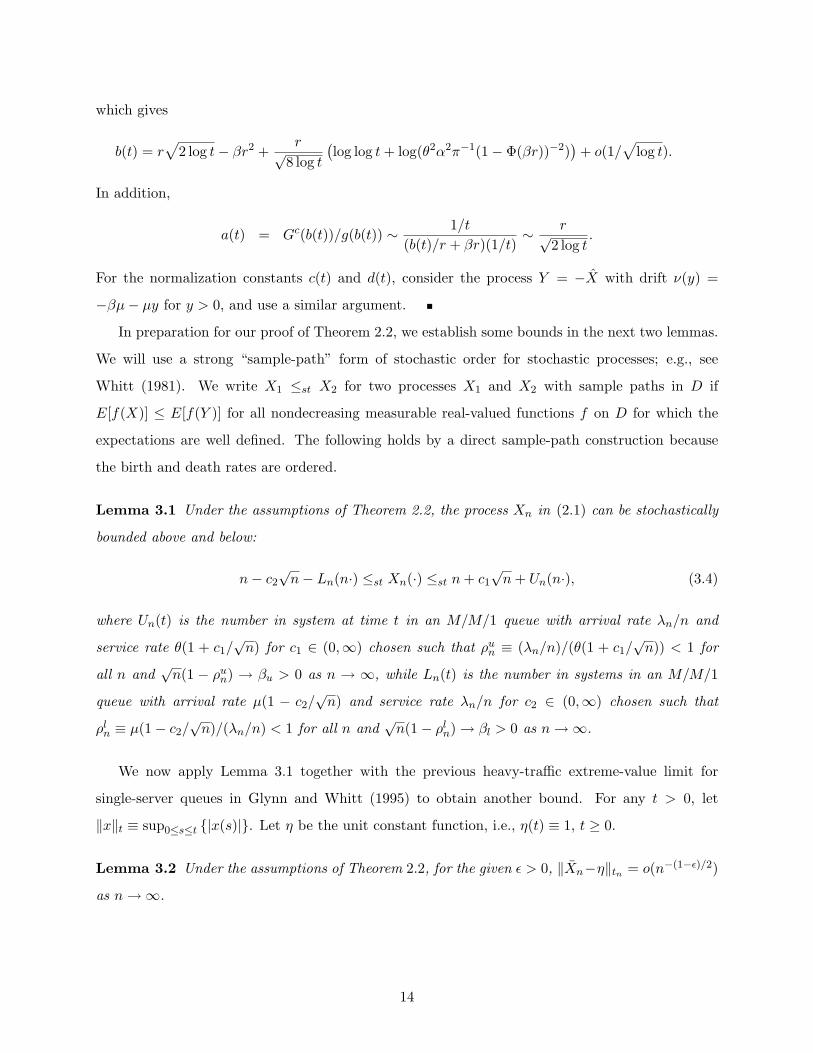
which gives

b(t) = r√

2 log t− βr2 +r√

8 log t

(log log t+ log(θ2α2π−1(1− Φ(βr))−2)

)+ o(1/

√log t).

In addition,

a(t) = Gc(b(t))/g(b(t)) ∼ 1/t(b(t)/r + βr)(1/t)

∼ r√2 log t

.

For the normalization constants c(t) and d(t), consider the process Y = −X with drift ν(y) =

−βµ− µy for y > 0, and use a similar argument.

In preparation for our proof of Theorem 2.2, we establish some bounds in the next two lemmas.

We will use a strong “sample-path” form of stochastic order for stochastic processes; e.g., see

Whitt (1981). We write X1 ≤st X2 for two processes X1 and X2 with sample paths in D if

E[f(X)] ≤ E[f(Y )] for all nondecreasing measurable real-valued functions f on D for which the

expectations are well defined. The following holds by a direct sample-path construction because

the birth and death rates are ordered.

Lemma 3.1 Under the assumptions of Theorem 2.2, the process Xn in (2.1) can be stochastically

bounded above and below:

n− c2√n− Ln(n·) ≤st Xn(·) ≤st n+ c1

√n+ Un(n·), (3.4)

where Un(t) is the number in system at time t in an M/M/1 queue with arrival rate λn/n and

service rate θ(1 + c1/√n) for c1 ∈ (0,∞) chosen such that ρun ≡ (λn/n)/(θ(1 + c1/

√n)) < 1 for

all n and√n(1 − ρun) → βu > 0 as n → ∞, while Ln(t) is the number in systems in an M/M/1

queue with arrival rate µ(1 − c2/√n) and service rate λn/n for c2 ∈ (0,∞) chosen such that

ρln ≡ µ(1− c2/√n)/(λn/n) < 1 for all n and

√n(1− ρln)→ βl > 0 as n→∞.

We now apply Lemma 3.1 together with the previous heavy-traffic extreme-value limit for

single-server queues in Glynn and Whitt (1995) to obtain another bound. For any t > 0, let

‖x‖t ≡ sup0≤s≤t {|x(s)|}. Let η be the unit constant function, i.e., η(t) ≡ 1, t ≥ 0.

Lemma 3.2 Under the assumptions of Theorem 2.2, for the given ε > 0, ‖Xn−η‖tn = o(n−(1−ε)/2)

as n→∞.

14

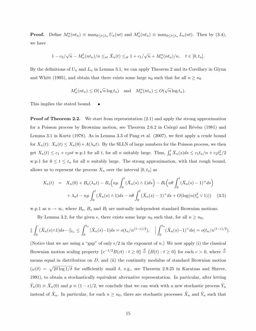
Proof. Define Mun (ntn) ≡ max0≤t≤tn Un(nt) and M l

n(ntn) ≡ max0≤t≤tn Ln(nt). Then by (3.4),

we have

1− c2/√n−M l

n(ntn)/n ≤st Xn(t) ≤st 1 + c1/√n+Mu

n (ntn)/n, t ∈ [0, tn].

By the definitions of Un and Ln in Lemma 3.1, we can apply Theorem 2 and its Corollary in Glynn

and Whitt (1995), and obtain that there exists some large n0 such that for all n ≥ n0

M ln(ntn) ≤ O(

√n log tn) and Mu

n (ntn) ≤ O(√n log tn).

This implies the stated bound.

Proof of Theorem 2.2. We start from representation (2.1) and apply the strong approximation

for a Poisson process by Brownian motion, see Theorem 2.6.2 in Csorgo and Revesz (1981) and

Lemma 3.1 in Kurtz (1978). As in Lemma 3.3 of Pang et al. (2007), we first apply a crude bound

for Xn(t): Xn(t) ≤ Xn(0)+A(λnt). By the SLLN of large numbers for the Poisson process, we then

get Xn(t) ≤ c1 + c2nt w.p.1 for all t, for all n suitably large. Thus,∫ t0 Xn(s)ds ≤ c1tn/n + c2t

2n/2

w.p.1 for 0 ≤ t ≤ tn for all n suitably large. The strong approximation, with that rough bound,

allows us to represent the process Xn over the interval [0, tn] as

Xn(t) = Xn(0) +Ba(λnt)−Bs(nµ

∫ t

0(Xn(s) ∧ 1)ds

)−Bl

(nθ

∫ t

0(Xn(s)− 1)+ds

)+ λnt− nµ

∫ t

0(Xn(s) ∧ 1)ds− nθ

∫ t

0(Xn(s)− 1)+ds+O(log(n(t2n ∨ 1))) (3.5)

w.p.1 as n→∞, where Ba, Bs and Bl are mutually independent standard Brownian motions.

By Lemma 3.2, for the given ε, there exists some large n0 such that, for all n ≥ n0,

‖∫ ·

0(Xn(s)∧1)ds−·‖tn ≤

∫ tn

0|Xn(s)−1|ds = o(tn/n(1−ε)/2),

∣∣∣ ∫ tn

0(Xn(s)−1)+ds| = o(tn/n(1−ε)/2).

(Notice that we are using a “gap” of only ε/2 in the exponent of n.) We now apply (i) the classical

Brownian motion scaling property {c−1/2B(ct) : t ≥ 0} d= {B(t) : t ≥ 0} for each c > 0, where d=

means equal in distribution on D, and (ii) the continuity modulus of standard Brownian motion

(ω(δ) =√

2δ log 1/δ for sufficiently small δ, e.g., see Theorem 2.9.25 in Karatzas and Shreve,

1991), to obtain a stochastically equivalent alternative representation. In particular, after letting

Yn(0) ≡ Xn(0) and p ≡ (1− ε)/2, we conclude that we can work with a new stochastic process Yn

instead of Xn. In particular, for each n ≥ n0, there are stochastic processes Xn and Yn such that

15

Xnd= Xn for each n,

‖Xn − Yn‖tn ≡ ∆n = O(((tn/np) log(np/tn))1/2 + (log nt2n)/

√n)

w.p.1 and (3.6)

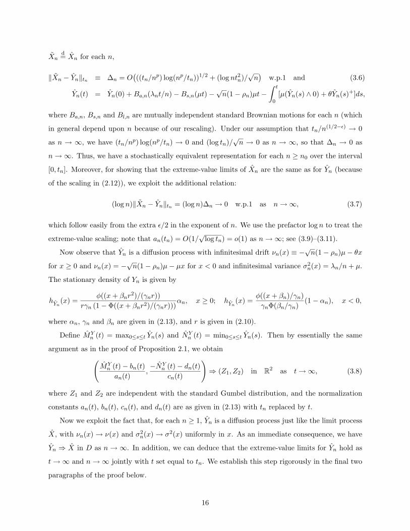
Yn(t) = Yn(0) +Ba,n(λnt/n)−Bs,n(µt)−√n(1− ρn)µt−

∫ t

0[µ(Yn(s) ∧ 0) + θYn(s)+]ds,

where Ba,n, Bs,n and Bl,n are mutually independent standard Brownian motions for each n (which

in general depend upon n because of our rescaling). Under our assumption that tn/n(1/2−ε) → 0

as n → ∞, we have (tn/np) log(np/tn) → 0 and (log tn)/√n → 0 as n → ∞, so that ∆n → 0 as

n→∞. Thus, we have a stochastically equivalent representation for each n ≥ n0 over the interval

[0, tn]. Moreover, for showing that the extreme-value limits of Xn are the same as for Yn (because

of the scaling in (2.12)), we exploit the additional relation:

(log n)‖Xn − Yn‖tn = (log n)∆n → 0 w.p.1 as n→∞, (3.7)

which follow easily from the extra ε/2 in the exponent of n. We use the prefactor log n to treat the

extreme-value scaling; note that an(tn) = O(1/√

log tn) = o(1) as n→∞; see (3.9)–(3.11).

Now observe that Yn is a diffusion process with infinitesimal drift νn(x) ≡ −√n(1− ρn)µ− θx

for x ≥ 0 and νn(x) = −√n(1− ρn)µ− µx for x < 0 and infinitesimal variance σ2

n(x) = λn/n+ µ.

The stationary density of Yn is given by

hYn(x) =

φ((x+ βnr2)/(γnr))

rγn (1− Φ((x+ βnr2)/(γnr)))αn, x ≥ 0; hYn

(x) =φ((x+ βn)/γn)γnΦ(βn/γn)

(1− αn), x < 0,

where αn, γn and βn are given in (2.13), and r is given in (2.10).

Define MYn (t) = max0≤s≤t Yn(s) and NY

n (t) = min0≤s≤t Yn(s). Then by essentially the same

argument as in the proof of Proposition 2.1, we obtain(MYn (t)− bn(t)an(t)

,−NY

n (t)− dn(t)cn(t)

)⇒ (Z1, Z2) in R2 as t→∞, (3.8)

where Z1 and Z2 are independent with the standard Gumbel distribution, and the normalization

constants an(t), bn(t), cn(t), and dn(t) are as given in (2.13) with tn replaced by t.

Now we exploit the fact that, for each n ≥ 1, Yn is a diffusion process just like the limit process

X, with νn(x)→ ν(x) and σ2n(x)→ σ2(x) uniformly in x. As an immediate consequence, we have

Yn ⇒ X in D as n→∞. In addition, we can deduce that the extreme-value limits for Yn hold as

t→∞ and n→∞ jointly with t set equal to tn. We establish this step rigorously in the final two

paragraphs of the proof below.

16

Next, the limit in (3.7), together with the fact that Xnd= Xn for each n, implies that the same

extreme-value limit holds for the scaled versions of Xn as n→∞ with tn →∞ at the specified rate.

We now give additional details. In particular, we now justify the claim that the scaling functions

can be switched in the way claimed. First, it is easy to see from (2.10) and (2.13) that an(t)→ a(t),

bn(t) → b(t), cn(t) → c(t), and dn(t) → d(t) as n → ∞ for each t. For the replacement of an(tn),

bn(tn), cn(tn) and dn(tn) by a(tn), b(tn), c(tn) and d(tn), respectively, in (2.12), some care is needed,

because b(tn)→∞ and a(tn)→ 0 as n→∞ (and similarly for c and d). We can write

Mn(tn)− bn(tn)an(tn)

=Mn(tn)− b(tn)

a(tn)[an(tn)/a(tn)]− bn(tn)− b(tn)a(tn)[an(tn)/a(tn)]

. (3.9)

First, an(tn)/a(tn)→ 1 as n→∞. Second,

bn(tn)− b(tn)a(tn)

= 2(γn − 1) log tn − r(βn − β)√

2 log tn +12

(γn − 1) log log tn (3.10)

+12

(γn − 1) log(θ2α2nπ−1(1− Φ(βnr/γn))−2)− 1

2log(α2n(1− Φ(βnr/γn))−2

α2(1− Φ(βr))−2

).

Note that, by (2.4), we have ρn = 1−O(1/√n), and γn =

√(ρn + 1)/2 = 1−O(1/

√n). Hence,

|γn − 1| log tn = O( log tn√

n

)→ 0 as n→∞. (3.11)

Consequently, all the terms in (3.10) are o(1) as n→∞.

Finally, we justify the joint limit as n → ∞ and t → ∞ in (3.8) where t = tn, satisfying the

growth assumption. We do so by bounding the processes Yn above and below by deterministic

modifications of the fixed limit process X. In particular, we establish the strong sample path

stochastic ordering

(1 + cn)X(t)− dlnt ≤st Yn(t) ≤st (1 + cn)X(t) + dunt, t ≥ 0, (3.12)

where cn, dln and dun are all constants depending on n, each being O(1/√n). We use the prefactor

(1+cn) to make the infinitesimal variance match the infinitesimal variance σ2n(x) = σ2

n of Yn. Then

we use the stochastic comparison of diffusion processes with common infinitesimal variance but

ordered drifts in Theorem 23.5 of Kallenberg (2002) to obtain the ordering in (3.12).

The starting point is the elementary observation that, if Z is a diffusion process with infinitesimal

mean function ν(x) and infinitesimal variance σ2(x), and c is a positive constant, then cZ(t) is

a diffusion process with infinitesimal mean function νc(x) = cν(x/c) and infinitesimal variance

function σ2c (x) = c2σ2(x/c). That applies conveniently in our case, because σ2(x) = σ2, a constant,

17

while ν(x) is composed of two linear pieces. Thus, in (3.12) we take 1 + cn =√σ2n/σ

2. That

yields (1 + cn)2 = σ2n/σ

2 = 1 +O(1/√n), which implies that cn = O(1/

√n). The infinitesimal drift

function for (1+cn)X is −(1+cn)µβn−θx for x ≥ 0 and −(1+cn)µβn−µx for x ≤ 0, which differs

from the infinitesimal mean function ν of X by a constant function of x depending on n. We can

now obtain the two bounds in (3.12) by subtracting and adding appropriate functions dnt. These

constants dln and dun are both O(1/√n) because cn = O(1/

√n) and βn − β = O(1/

√n). The proof

is completed by observing that the extreme-value limits for the bounds, setting t = tn, is the same

as for X itself, because tn/√n → 0 as n → ∞ under the assumption on the growth of tn. Hence,

the claim (2.12) is proved.

3.3 Sketch of the Remaining Proofs

Proof of Theorem 2.3. We can use the same argument as in the proof of Theorem 2.2 except

for the following points. First, by the known fluid limit, for any ε ∈ (0, (λ − µ)/θ), there exists

some n1 such that for all n ≥ n1, inf0≤t≤T XEDn (s) ≥ n(1 + (λ− µ)/θ − ε) > n, for any T > 0. So,

the strong approximation of XEDn in (3.5) simplifies,

XEDn (t) = XED

n (0) +Ba(nλt)−Bs(nµt)−Bl(nθ

∫ t

0(XED

n (s)− 1)ds)

+ nλt− nµt− nθ∫ t

0(XED

n (s)− 1)ds+O(log n(t2n ∨ 1)).

Second, as in Lemma 3.1, we can stochastically bound XEDn above and below, but now centering

around n(1 + (λ − µ)/θ) instead of around n, by two M/M/1 queues to obtain the same bound

for ||XEDn − η||tn as in Lemma 3.2. Third, paralleling (3.6), for each n ≥ n0, after letting Yn(0) ≡

XEDn (0) and p ≡ (1 − ε)/2, we observe that there are stochastic processes Xn and Yn such that

Xnd= XED

n for each n, ‖Xn − Yn‖tn ≡ ∆n as in (3.6), and

Yn(t) = Yn(0) +Ba.n(λt)−Bs,n(µt)−Bl,n((λ− µ)t)− θ∫ t

0Yn(s) ds.

However, now we find that Ynd= XED for each n, where XED is the OU process in (2.15). Hence

we can directly apply Proposition 3.1.

Proof of Proposition 2.2 We apply the argument used in the proof of Proposition 2.1. First,

the stationary density of X in (2.19) is given by

h(x) = βe−βxα, x ≥ 0 and h(x) =φ(β + x)

Φ(β)(1− α), x < 0, (3.13)

18

where α is given in (2.21). Then the tail of the distribution function F in (3.1) becomes

F c(x) ∼ β2µαe−βx ≡ Gc(x) ∼ 1−G(x) as x→∞.

Thus, the constants a(t) and b(t) given in Proposition 2.2 can be obtained by (3.3) where g(x) =

−dGc(x)/dx = βGc(x). Since − logGc(b(t)) = log t, we have − log(β2µα) + βb(t) = log t.

Proof of Theorem 2.4. Again, we can use the same argument as in the proof of Theorem 2.2

with minor modification. First, in Lemma 3.1, we only need to stochastically bound the process Xn

from below, which will result in the same bound as given in Lemma 3.2. Second, the stochastically

equivalent representation Yn in (3.6) becomes

Yn(t) = Yn(0) +Ba,n(λnt/n)−Bs,n(µt)−√n(1− ρn)µt− µ

∫ t

0(Yn(s) ∧ 0)ds,

with Yn(0) = Xn(0). In order to obtain the joint limit as n → ∞ and t → ∞ with t = tn, we can

again relate Yn to X in the same way. Third, the stationary density of Yn is given by

hYn(x) = αnβnγ

−2n exp

(−βnγ−2

n x), x ≥ 0, and hYn

(x) =φ((x+ βn)/γn)γnΦ(βn/γn)

(1− αn), x < 0,

where αn, βn and γn are given in (2.22). Then by the argument used to prove Proposition 2.1, we

obtain (3.8) where the normalization constants an(t), bn(t), cn(t) and dn(t) are given in (2.22) with

tn replaced by t.

References

[1] Artalejo, J.R., Economou, A., Gomez-Corral, A.: Applications of maximum queue lengths tocall center management. Computers and Operations Research. 34, 983–996 (2007)

[2] Artalejo, J.R., Economou, A., Lopez-Herrero, M.J.: Algorithmic analysis of the maximumqueue length in a busy period for the M/M/c retrial queue. INFORMS Journal on Computing.19, 121–126 (2007)

[3] Asmussen, S.: Extreme value theory for queues via cycle maxima. Extremes. 1:2, 137-168(1998)

[4] Billingsley, P.: Convergence of Probability Measures. second ed, Wiley, New York (1999)

[5] Borkovec, M., Kluppelberg, C.: Extremal behavior of diffusion models in finance. Extremes.1, 47–80 (1998)

[6] Browne, S., Whitt, W.: Piecewise-linear diffusion processes. Advances in Queueing, J. Dsha-lalow, ed., CRC Press, Boca Raton, FL, 463–480 (1995)

[7] Castillo, E.: Extreme Value Theory in Engineering, Academic Press, New York (1988)

19

[8] Csorgo, M., Revesz, P.: Strong Approximations in Probability and Statistics. Akademiai Kiado,Budapest. (1981)

[9] Darling, D.A., Erdos, P.: A limit theorem for the maximum of normalized sums of independentrandom variables. Duke Math. J. 23, 143–145 (1956)

[10] Davis, R.A.: Maximum and minimum of one-dimensional diffusions. Stochastic Processes andtheir Applications. 13, 1–9 (1982)

[11] Embrechts, P., Kluppelberg, C., Mikosch, T.: Modelling Extremal Events for Insurance andFinance. Springer, New York. (1997)

[12] Gans, N., Koole, G., Mandelbaum, A.: Telephone call centers: tutorial, review and researchprospects. Manufacturing and Service Operations Management. 5, 79–141 (2003)

[13] Garnett, O., Mandelbaum, A., Reiman, M. I.: Designing a call center with impatient cus-tomers. Manufacturing and Service Opns. Mgmt. 4, 208–227 (2002)

[14] Green, L. V., Kolesar, P. J., Whitt, W.: Coping with time-varying demand when settingstaffing requirements for a service system. Production and Operations Management. 16 13–39(2007)

[15] Glynn, P.W., Whitt, W.: Heavy-traffic extreme-value limits for queues. Operations ResearchLetters. 18, 107–111 (1995)

[16] Halfin, S., Whitt, W.: Heavy-traffic limits for queues with many exponential servers. Opera-tions Research. 29, 567–588 (1981)

[17] Kallenberg, O.: Foundations of Modern Probability. second ed., Springer, New York (2002)

[18] Karatzas, I., Shreve, S.E.: Brownian Motion and Stochastic Calculus. second ed., Springer,Berlin (1991)

[19] Kurtz, T.G.: Strong approximation theorems for density dependent Markov chains. StochasticProcesses and their Applications. 6, 223–240 (1978)

[20] Leadbetter, M.R., Lindgren, G., Rootzen, H.: Extremes and Related Properties of RandomSequences and Processes. Springer (1982)

[21] McCormick, W.P., Park, Y.S. Approximating the distribution of the maximum queue lengthfor M/M/s queues. Queues and Related Models. (V.N. Bhat and I.W. Basawa, eds.) OxfordUniversity Press, 240–261 (1992)

[22] Pang, G., Talreja, R., Whitt, W.: Martingale proofs of many-server heavy-traffic limits forMarkovian queues. Probability Surveys. 4, 193–267 (2007)

[23] Sadowsky, J., Szpankowski, W.: Maximum queue length and waiting time revisited: GI/G/cqueue. Probability in the Engineering and Information Sciences. 6, 157–170 (1995)

[24] Serfozo, R.F.: Extreme values of birth and death processes and queues. Stochastic Processesand their Applications. 27, 291–306 (1988)

[25] Whitt, W.: Comparing Counting Processes and Queues. Advances in Applied Probability. 13,207-220 (1981)

20

[26] Whitt, W.: Stochastic-Process Limits. Springer, New York (2002)

[27] Whitt, W.: Efficiency-driven heavy-traffic approximations for many-server queues with aban-donments. Management Science. 50, 1449–1461 (2004)

21