Hedge fund portfolio construction: A comparison of static and

dynamic approaches

Daniel Giamouridisa,∗, Ioannis D.Vrontosb

aDepartment of Accounting and Finance, Athens University of Economics and Business, Athens, Greece, andFaculty of Finance, Sir John Cass Business School, City University, London, UK

bDepartment of Statistics, Athens University of Economics and Business, Athens, Greece

Abstract

This article studies the impact of modelling time varying covariances/correlations of hedge fund

returns in terms of hedge fund portfolio construction and risk measurement. We use a variety of static and

dynamic covariance/correlation prediction models and compare the optimized portfolios’ out-of-sample

performance. We find that dynamic covariance/correlation models construct portfolios with lower risk

and higher out-of-sample risk-adjusted realized return. The tail-risk of the constructed portfolios is also

lower. Using a mean-conditional-value-at-risk framework we show that dynamic covariance/correlation

models are also successful in constructing portfolios with minimum tail-risk.

JEL classification : G11; G12

Keywords : Hedge fund portfolios; dynamic covariances/correlations; multivariate GARCH; regime

switching; CVaR

∗Corresponding author. Department of Accounting and Finance, Athens University of Economics and Business, Patission

76, GR-10434 Athens, Greece. Tel.: +30-210-8203925; fax: +30-210-8203936. Email: dgiamour@aueb.gr

1

1 Introduction

The hedge fund industry has been growing rapidly over the last years. Individual hedge funds and funds

of funds have been traditionally available to high net-worth individuals or institutional investors seeking

exposure in the so-called alternative investments arena. With the recent launch of investable hedge fund

indices, small- to medium-sized investors also gained access to this asset class, either directly or via index-

linked products1. These developments have attracted a substantial amount of business and give an additional

boost to interest in studying hedge fund investments.

To date research in hedge fund investing has mainly focused on determining the right proportion to

allocate in hedge funds (see, e.g. Terhaar et al., 2003, Cvitanic et al., 2003, Popova et al., 2003, Amin and

Kat, 2003), on identifying hedge fund risks (see, e.g. Fung and Hsieh, 1997, Ackermann et al., 1999, Brown

et al., 1999, Edwards and Caglayan, 2001, Liew, 2003, Agarwal and Naik, 2004), and on constructing optimal

hedge fund portfolios (see, e.g. McFall Lamm, 2003, Kat, 2004, Agarwal and Naik, 2004, Alexander and

Dimitriu, 2004, Morton et al., 2005). These studies, despite, (a) the nature of hedge fund investments i.e.

dynamic trading strategies, derivatives, and leverage used by fund managers, (b) the well known fact that

the variance and covariance of most financial time series - the funds’ underlying assets - are time-varying,

and (c) empirical evidence for volatility clustering and high kurtosis in the time series of fund returns (see,

e.g. McFall Lamm, 2003, Morton et al., 2005), do not account for possible time-varying variances and

covariances/correlations of hedge fund returns. They assume constant - static - covariance/correlation

structure through time. As a result hedge fund return variances and covariances/correlations may not be

measured accurately, with potential important impacts in terms of asset allocation, pricing, and portfolio

construction, but also in terms of risk measurement, i.e. computation of the Value at Risk (VaR), the

Conditional Value at Risk (CVaR).

In this paper, we address the issue of time-varying variances and covariances/correlations of hedge fund

returns and concentrate on the potential impacts in terms of hedge fund portfolio construction and risk

measurement. We start with the case where the hypothetical investor is concerned with the volatility1See Ferry (2004) and Walker and Butcher (2004) for a discussion of investable hedge fund index products.

2

of the portfolio. We compare the performance of different methods of forecasting variances and covari-

ances/correlations, with an eye to judge which model improves our ability to optimize hedge fund portfolio

risk. More specifically we compare the performance of five different forecasting models: (a) a sample co-

variance model, (b) an implicit factor model (Fung and Hsieh, 1997, Amenc and Martellini, 2002, Alexander

and Dimitriu, 2004), (c) an implicit factor GARCH model (Alexander, 2001), (d) an implicit full-factor

GARCH model (Vrontos et al., 2003), and (e) a regime switching dynamic correlations model (Pelletier,

2005). The different models are evaluated, out-of-sample, in a case study which examines the portfolio risk,

but also realized return, risk-adjusted realized return, and tail-risk. We then hypothesize that the investor

is concerned with the portfolio tail-risk. We set up an additional case study where the different risk models

are evaluated, out-of-sample, for their ability to construct hedge fund portfolios with optimal tail-risk.

Our empirical analysis provides three main findings. First, we find that dynamic covariance/correlation

prediction models improve our ability to optimize hedge fund portfolios. They are able to construct portfolios

with lower average risk and higher average risk-adjusted realized return. These results are significant on

a statistical basis. Second, we find that the dynamic models provide a more accurate tool for tail-risk

measurement. They are able to construct hedge fund portfolios which exhibit significantly lower tail-risk.

Third, we find that the allocation determined by the dynamic covariance/correlation prediction models is

not very similar with that computed from the other models. In fact, this difference is substantial for

certain funds, suggesting that a more accurate risk model improves our ability to select the right fund for

the portfolio. Our findings have important implications for hedge fund style allocation decisions and risk

measurement. They also provide useful insights for managers wishing to adopt a dynamic approach for fund

selection and allocation purposes.

The contributions of this article are several. We model time-varying covariances/correlations of hedge

fund returns for the first time to our knowledge. In the dynamic environment that hedge fund investments

are determined, variances and covariances/correlations are expected to change over time, thus, making it

sensible to seek an appropriate covariance specification in this class of models. In addition, we perform a

comparative study to evaluate the ability of different covariance prediction models to construct optimal hedge

3

fund portfolios. This analysis is executed out-of-sample and the results are validated on a statistical basis.

Also, we provide a thorough analysis of coherent tail-risk measures. Hedge fund tail-risk measurement is

of particular importance given the impact of extreme events in hedge fund investments. Agarwal and Naik

(2004) and Krokhmal et al. (2002) are the only studies we know of that touch upon the issue of hedge fund

portfolio tail-risk measurement. We extend their analysis in that we measure hedge fund portfolio tail-risk for

a number of different covariance/correlation models. The entire study is carried out on portfolios constructed

with different optimization benchmarks to study performance under different investment objectives. The

sensitivity of our conclusions to the choice of parameters such as the rebalancing frequency or the size of the

estimation period is also examined. This analysis is also new, to our knowledge, to the hedge fund portfolio

construction literature.

The remainder of this article proceeds as follows. Section 2 discusses the approaches used to construct

optimal hedge fund portfolios. Section 3 outlines the covariance prediction models used in our empirical

analysis. Section 4 discusses the data. Section 5 presents the metrics used in our empirical analysis and

reports the results of our investment exercise. Section 6 concludes.

2 Optimal hedge fund portfolios

The standard Markowitz (1952) mean-variance analysis in the construction of portfolios involving hedge

funds has been subject to criticisms in the literature. While Amenc and Martellini (2002), Terhaar et

al. (2003), Alexander and Dimitriu (2004) concentrate on hedge fund allocation within mean-variance

opportunity sets, alternative approaches have been proposed. Barès et al. (2002) and Cvitanic et al.

(2003), for example, determine the optimal asset allocation in an expected utility framework. Amin and

Kat (2003) discuss the issues arising in mean-variance allocation when the distribution of asset returns is

not symmetric. Popova et al. (2003), Hagelin and Pramborg (2003), and Davies et al. (2005) deal with

these issues by employing higher moment analysis. McFall Lamm (2003) also addresses asymmetry and

fat-tailness in the returns distributions with Duarte’s (1999) generalized approach. Krokhmal et al. (2002),

on the other hand, construct optimal portfolios using alternative - to the standard variance - risk objectives

4

which control different types of risks, i.e. CVaR and CDaR (Conditional Drawdown at Risk) among others.

In the same vain, Agarwal and Naik (2004) seek optimal mean-CVaR portfolios. Finally, Rockafellar et al.

(2005) propose generalized measures as substitutes for standard deviation.

The criticisms against the mean-variance framework stress that it is appropriate only for normally dis-

tributed returns or for investors having quadratic preferences, thus, making it not perfectly applicable to

hedge funds. Chambers and Quiggin (2005), however, prove that ‘...much of the standard mean-standard

deviation analysis can be extended to general invariant preferences, without requiring...[the preferences to

be]...neutral with respect to...higher moments’. In addition to that, the mean-variance analysis is a widely

used portfolio construction approach in practice. We, thus, focus on the mean-variance approach and in-

vestigate if an appropriate covariance model improves our ability to construct optimal portfolios. In the

mean-variance framework portfolios are constructed through the following optimization:

minXV ar(Rp) (1)

s.t. xi > 0, i = 1, ..., n,nXi=1

xi = 1, and E (Rp) > T arg et return

where Rp and V ar(Rp)(= X0VX) are the n−assets hedge fund portfolio return and variance respectively,

X =(x1, x2, ..., xn)0 is the vector containing the funds’ weights in the portfolio, V is the n × n covariance

matrix, and E (Rp) is the expected return of the fund portfolio. We impose no-short-sales constraints since

hedge funds cannot be shorted in practice.

Optimal portfolios can alternatively be constructed using other risk objectives. Given the increasing

emphasis on risk management and its potential payoffs, there is a proliferation of measures capturing different

types of risks. One such measure is the CVaR - the expectation of the losses greater than or equal to the

VaR - which measures the risk in the tail of the loss distribution. Krokhmal et al. (2002) employ a

number of risk management methodologies to construct optimal hedge fund portfolios. They conclude that

CVaR demonstrates the most solid out-of-sample performance in their data set. We also investigate how

alternative econometric specifications perform in constructing hedge fund portfolios with minimum tail risk.

We employ Rockafellar and Uryasev’s (2000) convex programming formulation. The problem is expressed

5

mathematically as follows:

minXCV aR(FRp ,α) (2)

s.t. xi > 0, i = 1, ..., n,nXi=1

xi = 1, and E (Rp) > T arg et return

where:

CVaR(FRp ,α) = −E(Rp |Rp ≤ −VaR) = −R −VaR−∞ zfRp(z)dz

FRp(−VaR)(3)

VaR(F eRp ,α) = −F−1Rp (1− α), fRp and FRp denote the probability density and the cumulative density of Rp

respectively, and α is a probability level. Rockafellar and Uryasev (2002) provide a thorough analysis of the

properties of CVaR in risk measurement and portfolio optimization exercises.

3 Predicting hedge fund return covariances

Given our focus on hedge fund portfolio risk or tail-risk optimization, we concentrate on predicting fund

return covariances. The fact that hedge fund investments are determined in a dynamic manner makes fund

returns and covariances modelling not a straightforward task. In addition to that, a short history of data is

normally available for hedge funds, thus, making the estimation of data-demanding models not always easy.

The ‘cleaning’ of the covariance matrix by imposing some structure is the common thread in the literature.

Amenc and Martellini (2002) discuss the trade-off between model risk and estimation risk in alternative

approaches. Explicit factor models (e.g. Agarwal and Naik, 2004) are claimed to involve high specification

error and low sampling error while models imposing optimal structure (e.g. Ledoit and Wolf, 2003) engage

medium, specification and sampling, errors. An alternative option is to use implicit factors. Amenc and

Martellini (2002) discuss the advantages of using implicit factor models. These involve low specification

error, as they exploit the information contained in the empirical correlation, and low sampling error due to

the - little - structure that is imposed.

Our empirical investigation uses a variety of covariance models including static and dynamic specifica-

tions. The static specifications include the sample covariance model and an implicit factor model which

has been used successfully in hedge fund pricing and portfolio construction studies (Fung and Hsieh, 1997,

6

Amenc and Martellini, 2002, Alexander and Dimitriu, 2004). A natural step towards dynamic modeling is

to consider an implicit factor GARCH model, which essentially models each factor as a GARCH processes

(Alexander, 2001). To model time-varying covariances/correlations we consider two additional dynamic

specifications. The full-factor multivariate GARCH model proposed by Vrontos et al. (2003) which falls

in the class of implicit factor models; and the regime switching dynamic correlations model proposed by

Pelletier (2005) which is a successful alternative - to GARCH models - for modeling conditional covari-

ances/correlations. The following paragraphs present the details of each model.

Throughout the paper we consider having observed returns

Rt, t = 1, ..., T

where each

Rt = (R1, R2, ..., Rn)0t

is a n× 1 vector of hedge fund returns in period t.

3.1 Sample covariance model

The sample covariance matrix during the estimation period corresponds to the basis model (SAM hereafter)

for our analysis. The sample covariance matrix is calculated through:

VSAM =1

T − 1

TXt=1

(Rt − R)(Rt − R)0 (4)

where T is the sample size and R is a n× 1 vector containing the means of the return vectors. This model

involves low specification error and high sampling error (Amenc and Martellini, 2002).

3.2 Implicit factor model

An implicit factor model involves extracting explanatory factors through principal components analysis of

the funds’ returns data. With n fund return series under study there are n principal components, and

these principal components are just linear combinations of the fund returns. The principal components are

7

constructed to be orthogonal to each other and to be normalized to have unit length. The implicit-factor

model (IFAC hereafter) is formulated as follows (see, Zivot and Wang, 2002):

Ri,t = αi +KXk=1

βikfk,t + εi,t (5)

where αi is a constant term, βik is the loading on factor k for the return of asset i, fk,t = R0tx∗k, k = 1, ...,K,

x∗k is the kth (n × 1) eigenvector of the return covariance matrix. We select the number of principal

components, K, so that at least 85% of the covariation in the portfolio is explained. Amenc and Martellini

(2002) discuss alternative approaches for selecting K. The covariance matrix of returns on a set of n hedge

funds, VIFAC , is given by:

VIFAC = BΩIFACB0 +D (6)

where B is the matrix of factor loadings, ΩIFAC is the diagonal covariance matrix of the implicit factors

and D is a diagonal matrix with elements in the main diagonal σ2i = var(εi,t).

3.3 Implicit factor GARCH model

A modification of the standard implicit factor model has been proposed by Alexander (2001) to benefit from

the success of GARCH models in financial markets volatility forecasting. In Alexander’s (2001) spirit, we

use principal component analysis to extract key implicit risk factors and estimate their volatilities on the

basis of a univariate GARCH model. Given a GARCH (1,1) representation the variances of the implicit

factors at time t are defined by:

σ2k,t = ωk + γkf2k,t−1 + δkσ

2k,t−1, k = 1, ...,K, t = 1, ..., T (7)

where ω > 0, and γ, δ ≥ 0. The implicit factor GARCH models (IFAC-G hereafter) follows the formulation

of Equation (5). The covariance matrix of the returns on a set of n hedge funds, VIFAC−Gt , is given by:

VIFAC−Gt = BΩIFAC−Gt B0 +D (8)

where ΩIFAC−Gt is a diagonal covariance matrix containing the GARCH variances given by Equation (7).

8

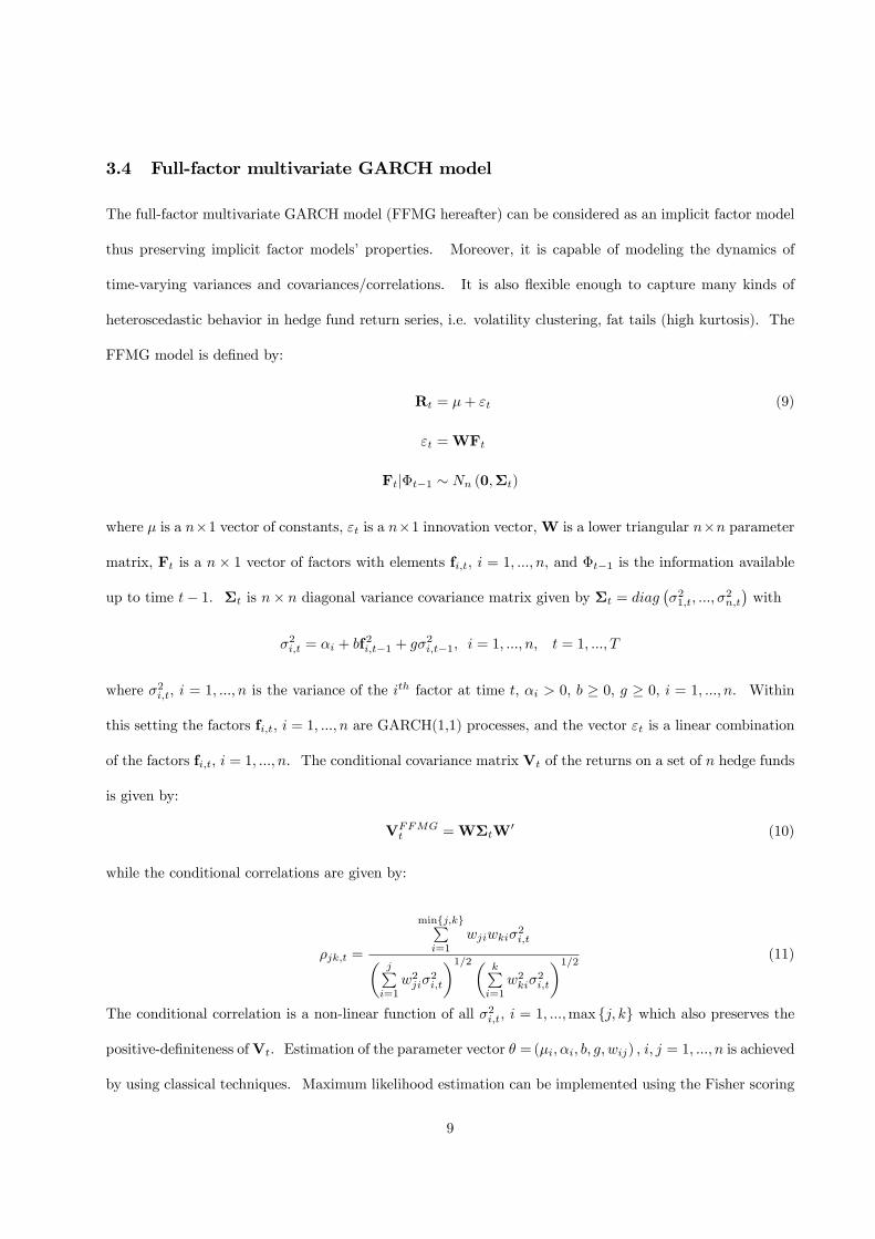
3.4 Full-factor multivariate GARCH model

The full-factor multivariate GARCH model (FFMG hereafter) can be considered as an implicit factor model

thus preserving implicit factor models’ properties. Moreover, it is capable of modeling the dynamics of

time-varying variances and covariances/correlations. It is also flexible enough to capture many kinds of

heteroscedastic behavior in hedge fund return series, i.e. volatility clustering, fat tails (high kurtosis). The

FFMG model is defined by:

Rt = µ+ εt (9)

εt =WFt

Ft|Φt−1 ∼ Nn (0,Σt)

where µ is a n×1 vector of constants, εt is a n×1 innovation vector,W is a lower triangular n×n parameter

matrix, Ft is a n× 1 vector of factors with elements fi,t, i = 1, ..., n, and Φt−1 is the information available

up to time t− 1. Σt is n× n diagonal variance covariance matrix given by Σt = diag¡σ21,t, ...,σ

2n,t

¢with

σ2i,t = αi + bf2i,t−1 + gσ

2i,t−1, i = 1, ..., n, t = 1, ..., T

where σ2i,t, i = 1, ..., n is the variance of the ith factor at time t, αi > 0, b ≥ 0, g ≥ 0, i = 1, ..., n. Within

this setting the factors fi,t, i = 1, ..., n are GARCH(1,1) processes, and the vector εt is a linear combination

of the factors fi,t, i = 1, ..., n. The conditional covariance matrix Vt of the returns on a set of n hedge funds

is given by:

VFFMGt =WΣtW

0 (10)

while the conditional correlations are given by:

ρjk,t =

minj,kPi=1

wjiwkiσ2i,tµ

jPi=1w2jiσ

2i,t

¶1/2µkPi=1w2kiσ

2i,t

¶1/2 (11)

The conditional correlation is a non-linear function of all σ2i,t, i = 1, ...,max j, k which also preserves the

positive-definiteness ofVt. Estimation of the parameter vector θ =(µi,αi, b, g, wij) , i, j = 1, ..., n is achieved

by using classical techniques. Maximum likelihood estimation can be implemented using the Fisher scoring

9

algorithm, since the gradient and the expected information matrices are available in closed form. A detailed

discussion of the theoretical as well as the empirical properties of the FFMG model can be found in Vrontos

et al. (2003).

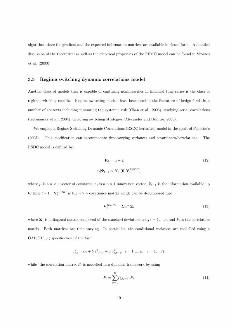
3.5 Regime switching dynamic correlations model

Another class of models that is capable of capturing nonlinearities in financial time series is the class of

regime switching models. Regime switching models have been used in the literature of hedge funds in a

number of contexts including measuring the systemic risk (Chan et al., 2005), studying serial correlations

(Getmansky et al., 2004), detecting switching strategies (Alexander and Dimitiu, 2005).

We employ a Regime Switching Dynamic Correlations (RSDC hereafter) model in the spirit of Pelletier’s

(2005). This specification can accommodate time-varying variances and covariances/correlations. The

RSDC model is defined by:

Rt = µ+ εt (12)

εt|Φt−1 ∼ Nn¡0,VRSDC

t

¢where µ is a n× 1 vector of constants, εt is a n× 1 innovation vector, Φt−1 is the information available up

to time t− 1. VRSDCt is the n× n covariance matrix which can be decomposed into

VRSDCt = ΣtPtΣt (13)

where Σt is a diagonal matrix composed of the standard deviations σi,t, i = 1, ..., n and Pt is the correlation

matrix. Both matrices are time varying. In particular, the conditional variances are modelled using a

GARCH(1,1) specification of the form

σ2i,t = αi + biε2i,t−1 + giσ

2i,t−1, i = 1, ..., n, t = 1, ..., T

while the correlation matrix Pt is modelled in a dynamic framework by using

Pt =KXk=1

ISt=kPk (14)

10

where I is the indicator function, St is an unobserved Markov chain process independent of εt which can

take K possible values (St = 1, 2, ...,K) and Pk are correlation matrices with Pk 6= Pk0 for k 6= k0. Regime

switches in the state variable, St, are assumed to be governed by the transition probability matrix Π. The

transition probabilities between states are assumed to follow a first order Markov chain and remain constant

through time:

Pr(St = j|St−1 = i, St−2 = l, ...) = Pr(St = j|St−1 = i) = πij , i, j = 1, ...,K

We assume K = 2. The estimation of the RSDC model is achieved by using a two-step procedure (Engle,

2002). In the first step we estimate the univariate GARCH model parameters and in the second step we

estimate the parameters in the correlation matrix and the transition probabilities πij conditional on the first

step estimates. Details of the estimation procedure can be found in Pelletier (2005).

4 The data

We carry out our empirical investigation by using hedge fund index data from Hedge Fund Research (HFR

hereafter). This choice makes our empirical analysis more relevant to style allocation decisions as in Amenc

and Martellini (2002), McFall Lamm (2003), Agarwal and Naik (2004) and Morton et al. (2005). We

consider eight HFR single strategy indices: Equity Hedge, Macro, Relative Value Arbitrage, Event-Driven,

Convertible Arbitrage, Distressed Securities, Equity Market Neutral, and Merger Arbitrage2. The sample

consists of monthly returns from January 1990 through to August 2005. It includes a number of crises that

occurred in the ’90s, i.e. the Mexican, Asian, Russian, the LTCM crises as well as the IT bubble and the

corporate scandals periods of the early ’00s. Crises cause large volatility variation and high kurtosis in the

returns data.

INSERT TABLE 1 ABOUT HERE

Table 1 reports summary statistics for the HFR single strategy hedge fund index returns over the period

of our analysis. Panel A in particular presents the mean, standard deviation, median, interquartile range,2These are the 8 single strategy indices for which HFR constructs investable counterparts called ‘HFRX investable strategy

indices’. Details can be found in www.hfr.com.

11

skewness, kurtosis, minimum, and the maximum for fund index returns. We observe thast the returns of the

eight hedge fund strategies are very heterogeneous: there are strategies with relatively high volatilities and

high average returns i.e. the Equity Hedge, Macro, Event Driven, and the Distressed Securities strategies.

Amenc and Martellini (2002) highlight that these strategies act as return enhancers and could substitute

some fraction of the portfolio’s equity holding. The Relative Value Arbitrage, Convertible Arbitrage, Equity

Market Neutral, and the Merger Arbitrage strategies exhibit low volatilities and low average returns. They

could be used in a portfolio to substitute some percentage of the fixed income or cash holdings. Differences

in the higher order moments are also present. The kurtosis of the eight indexes’ returns ranges from 3.34

to 14.29, indicating fat-tailness in most of the return distributions. Panel B reports correlation coefficients

computed for the HFR single strategy hedge fund index returns. We find that fund returns exhibit low to

medium pairwise correlation in general. This is a desirable property in the context of efficient portfolio

construction. Fund returns correlations range from a minimum of 0.17 between Equity Market Neutral

and Distressed Securities, to a maximum of 0.79 for Event Driven and Distressed Securities. The average

pairwise correlation is 0.47. Low correlation indicates a potential for risk diversification in hedge fund

investment portfolios.

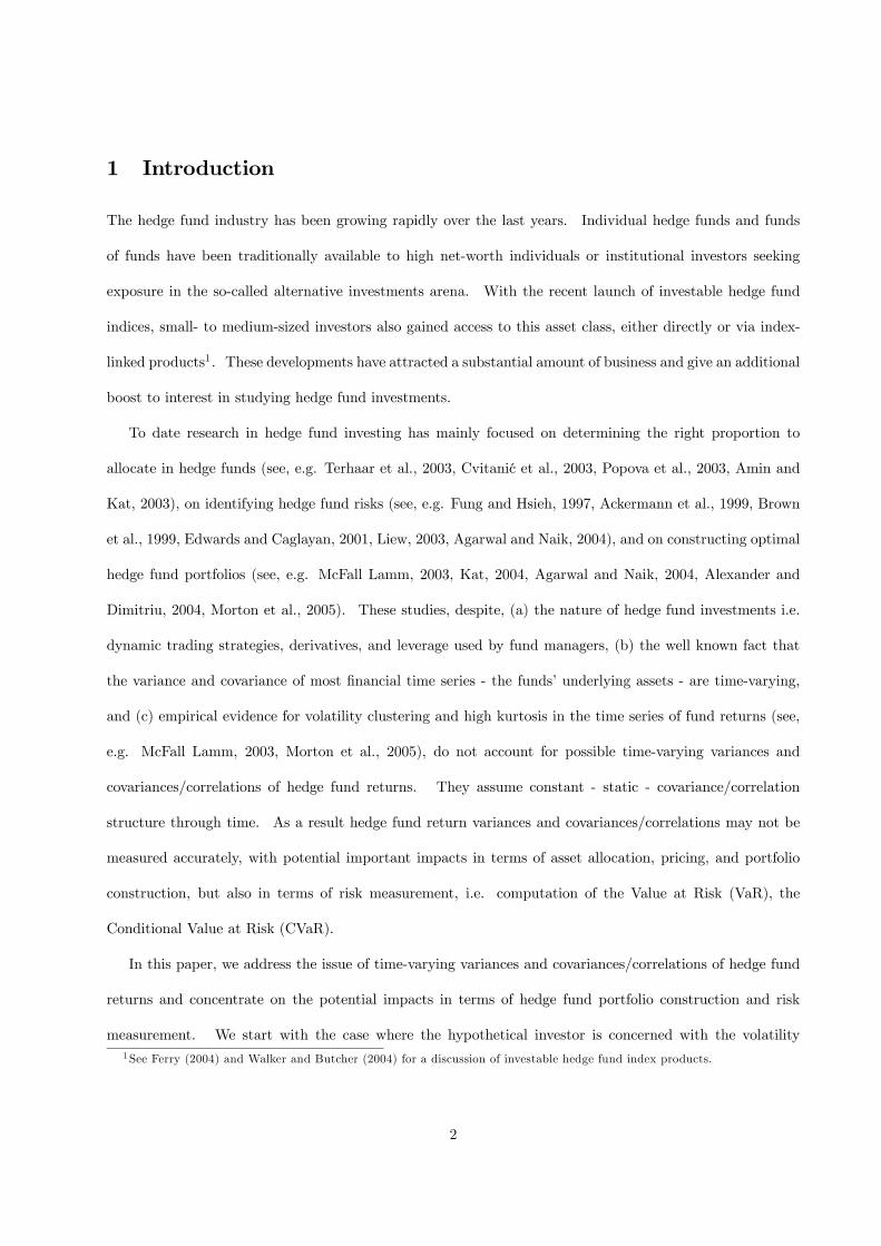
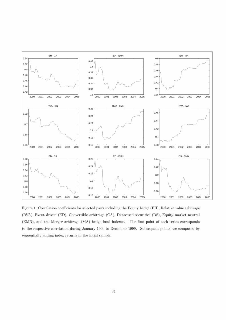
High kurtosis in hedge fund returns motivates, in principle, the use of dynamic covariance specifications.

Further analysis of the data reveals time-variation of covariances and correlations, thus, providing additional

support for the use of dynamic covariance/correlation models. To examine the variation of pairwise corre-

lations through time, we consider the data covering the period January 1990 through to December 1999 and

compute pairwise correlations. By sequentially adding index returns of subsequent months in the initial

dataset we compute a series of 68 correlation coefficients for each possible pair. Figure 1 plots correlation

coefficients for selected index pairs. We observe that pairwise correlations vary through time suggesting

that modeling time-varying correlations may improve our ability to construct optimal portfolios. Within

the set of models we compare, time-varying correlations can be modeled only with the FFMG specification

(see Equation 11) or with the RSDC model (see Equation 14).

INSERT FIGURE 1 ABOUT HERE

12

Our preliminary analysis of the data concludes that hedge fund index returns generally exhibit high kur-

tosis and time-varying variances and covariances/correlations. These findings motivate the use of dynamic

covariance/correlation specifications such as the FFMG and the RSDC.

5 Hedge fund portfolio performance

The objective of this study is to examine the benefits of introducing dynamic structures for the variances and

covariances/correlations of hedge fund returns in hedge fund portfolio construction and risk measurement.

This is achieved through an investment exercise which compares the empirical out-of-sample performance of

the different methods of forecasting variances and covariances/correlations presented in Section 3. The setup

of our experiments is as follows. We use a history of data covering the period January 1990 to December

2001 to estimate the parameters of the SAM, IFAC, IFAC-G, FFMG, and RSDC covariance matrixes. This

period contains 144 return observations for each asset. We then construct optimal hedge fund portfolios.

Two portfolios are constructed: (a) a conservative (no average annual return target - minimum variance

portfolio3), and (b) an aggressive (average annual return target of 15.5%). Given the optimized weights

we calculate buy-and-hold returns on the portfolio for a holding period of 1 month, at the end of which the

estimation and optimization procedures are repeated until the dataset is exhausted. The estimation period

grows by one data point every time we perform the optimization as in Krokhmal et al. (2002) in order to

utilize all available information. This exercise produces 44 out-of-sample observations that cover a period

of just over three and a half years, January 2002 to August 2005.

We assess the empirical performance of the covariance prediction models on several grounds.

First, we examine the realized returns of the constructed portfolios. Given the fund weightsXt=(x1, x2, ..., xn)0t

at time t and the realized returns of the individual n assets at time t+1 in our sample,Rt+1 = (R1, R2, ..., Rn)0t+1,

the realized return Rp of the portfolio at time t+ 1 is computed as3This portfolio requires no estimate of the expected return, thus, allowing performance evaluation of competing covariance

matrix estimators alone. For a discussion of this issue see Chan et al. (1999), for traditional assets, and Amenc and Martellini

(2002), Alexander and Dimitriu (2004) for alternative investments.

13

Rp,t+1 = X0tRt+1

We also calculate and discuss the cumulative returns for the entire period.

Second, we compare the return per unit of risk. Portfolio optimization will generally arrive at a different

minimum variance for each covariance prediction model. As a result the realized return will not be com-

parable across models since it will represent portfolios bearing different risk. We define a measure similar

in spirit to the Sharpe Ratio by standardizing the realized returns with the risk of the portfolio when it is

constructed. We call this measure a Conditional Sharpe Ratio (CSR hereafter) and calculate it through:

CSRp,t+1 =Rp,t+1pV ar(Rp)t

where V ar(Rp)t is determined through Equation 1.

Next, we set out to incorporate transaction costs. Transaction costs associated with hedge funds,

however, are not generally easy to compute given the variation in early redemption, management or other

types of fees (Alexander and Dimitriu, 2004). Nevertheless, if the gain in the performance does not cover

the extra transaction costs, less accurate, but less variable weighting strategies would be preferred. To study

this issue we define portfolio turnover as (Greyserman et al., 2005):

PTt+1 =nXi=1

|wi,t+1 − wi,t|

that is, the portfolio turnover in a given month is the sum of the absolute changes in the portfolio weights

from the previous month to that month. This metric intuitively represents the fraction (in percentage terms)

of the portfolio value that has to be liquidated/reallocated at the point of rebalancing.

Finally, we investigate the capacity of the different covariance prediction models to assess tail-risk. Agar-

wal and Naik (2004) focus on CVaR as a superior risk management tool to control the tail risk. The intuition

of CVaR is as follows. Suppose a hedge fund portfolio is managing $1 billion. A CVaR of 1% at the 95%

confidence level means that there is 5% probability that the average portfolio loss greater than or equal to

the VaR can exceed $10 million. A relatively higher CVaR, 1.1% for example, calculates the same loss as

14

$11 million which suggests an economically significant difference. To compute CVaR in Equation 3, one

can either impose a distributional assumption on the fund returns or use the empirical distribution of fund

returns. We include both approaches in our analysis. We assume that portfolio returns follow a multivariate

normal distribution with means and covariances determined by the respective covariance model. We also

calculate CVaR by using the empirical distribution. The CVaR is calculated at the 90%, 95%, and 99%

confidence levels.

Sections 5.1 and 5.2 present the results of two distinct case studies: the mean-variance case study and

the mean-CVaR case study.

In the mean-variance case study optimal portfolios are constructed with the (a) sample covariance model,

SAM, (b) implicit factor model, IFAC, (c) implicit factor GARCH model, IFAC-G, (d) full-factor multivariate

GARCH model, FFMG, and (e) the regime switching dynamic correlations model, RSDC. The sample

covariance model produces mean-variance portfolios whose weights are independent of the distributional

assumption on the fund returns. As a result all performance metrics are also independent of the distributional

assumption. Given the two approaches in CVaR calculation, however, the CVaR is calculated under the

empirical distribution (this model is termed SAM-E), but also under the multivariate normal distributional

assumption (this model is termed SAM-N).

In the mean-CVaR case study portfolios are constructed only with the sample covariance model and the

empirical distribution of hedge fund returns. Rockafellar and Uryasev (2000) show that for normal loss

distributions the mean-CVaR methodology is equivalent to the standard mean-variance approach. As a

result the portfolios constructed in the mean-variance case study with returns assumed multivariate normal

are also mean-CVaR optimal portfolios and can be used for comparison in this case study.

5.1 Out-of-sample performance of mean-variance optimal portfolios

Table 2 reports results of the out-of-sample performance of mean-variance efficient portfolios. Panel A,

provides average and median values of the metrics presented above, calculated in the conservative portfolio

construction exercise. Panel B, presents the average and median metrics’ values from the aggressive portfolio

15

construction exercise. Differences in the mean and median values of the metrics are examined through

standard t- and Wilcoxon signed-rank tests. Table 3 presents results of these tests for mean and median

‘CSR’. Due to space limitations the remaining results of the t- and Wilcoxon signed-rank tests are not

presented in detail.

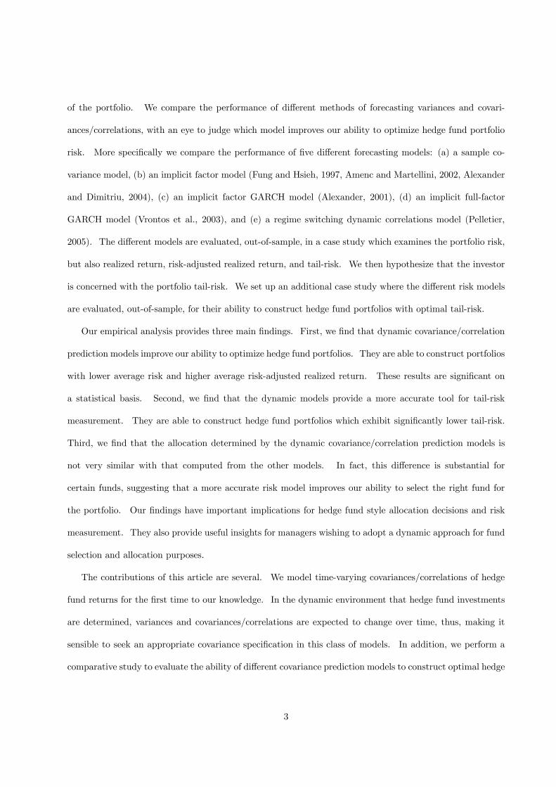
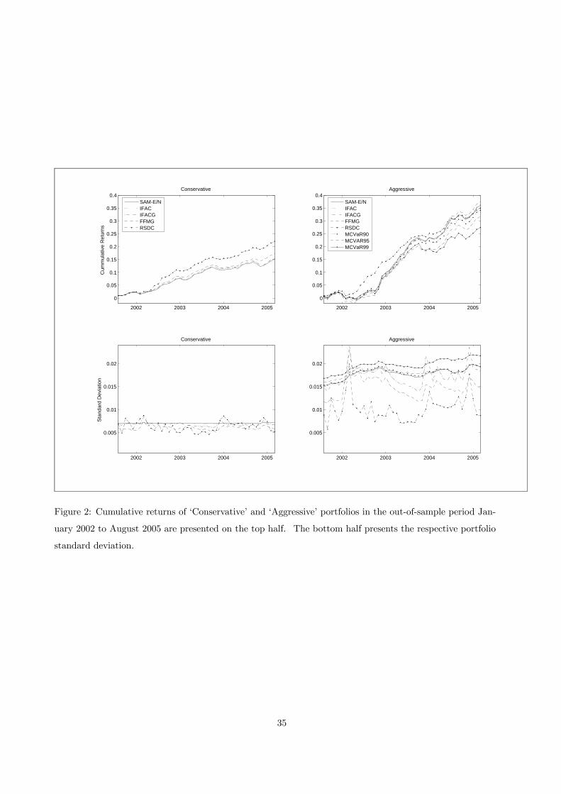
First, we examine portfolio performance in terms of the cumulative returns. The top half of Figure

2 plots cumulative returns of the conservative and the aggressive portfolios in the out-of-sample period.

The respective portfolio standard deviation is depicted on the bottom half of Figure 2. We find that

the RSDC covariance prediction model determines the conservative structure with the highest cumulative

return, 22.02%. The second best model for constructing conservative portfolios is the FFMG with out-of-

sample cumulative return of 17.25%. The IFAC-G and IFAC covariance models achieve 15.37% and 15.29%

respectively. The SAM cumulative returns are 14.95%. For aggressive portfolio construction, the FFMG

model ranks first with a cumulative return of 37.52%, followed by IFAC with 36.17%, IFAC-G with 36.04,

SAM with 35.98%, and RSDC with 34.95%. We should note here that this comparison penalizes models

with low realized returns ignoring the risk of the constructed portfolios.

INSERT FIGURE 2 ABOUT HERE

INSERT TABLE 2 ABOUT HERE

Next, we focus on ‘Return’, ‘Risk’, and ‘CSR’. Table 2 reports mean and median values of these metrics.

For the conservative portfolio construction exercise we find that the RSDC model computes structures that

realize the highest average and median out-of-sample ‘Return’. The second best model is the FFMG. In

terms of average and median ‘Risk’, FFMG ranks first and RSDC second. The ‘CSR’, ranks RSDC first

and FFMG second. IFAC-G ranks third by means of ‘Return’, ‘Risk’, and ‘CSR’. Examination of the

significance of the difference in the mean and median metrics’ values yields the following. The mean and

median ‘Return’ of RSDC are statistically different from all other models’. The mean and median ‘Return’

of FFMG are also statistically different from all other models’. The mean and median ‘Return’ of IFAC and

IFAC-G are not significantly different but are both different from SAM. The mean and median ‘Risk’ of

RSDC are not different from the mean and median ‘Risk’ of FFMG but are different all other models’. The

16

mean and median ‘CSR’ are statistically different in all models. For the aggressive portfolio construction

exercise we find that the mean and median ‘Return’ is the same for all models. The mean ‘Risk’ of RSDC

is statistically different from the mean ‘Risk’ of all other models. The same holds for the mean ‘Risk’ of

FFMG. The mean ‘Risk’ of IFAC-G, IFAC, and SAM are not statistically different. The median ‘Risk’ is

different in all models. The mean ‘CSR’ is statistically different in all models. The median ‘CSR’ is the

same for IFAC-G, IFAC, and SAM, but is different for RSDC and FFMG.

INSERT TABLE 3 ABOUT HERE

We also compare the capacity of the different covariance prediction models to assess tail risk and construct

optimal portfolios with minimal tail risk. In line with Agarwal and Naik (2004), we compute the 90%, 95%,

and 99% CVaR of mean-variance optimal portfolios and report mean and median values in Table 2. Mean

and median CVaR are consistently lower when the RSDC specification is used. FFMG ranks second and

IFAC-G third. For conservative portfolios we find that the mean and median 90%, 95%, and 99% CVaR

are significantly different in all models. For aggressive portfolios we find that the mean 90%, 95%, and

99% CVaR of RSDC are different from FFMG’s and are both different from the means of all other models.

Median 90%, 95%, and 99% CVaR, however, are significantly different in all models.

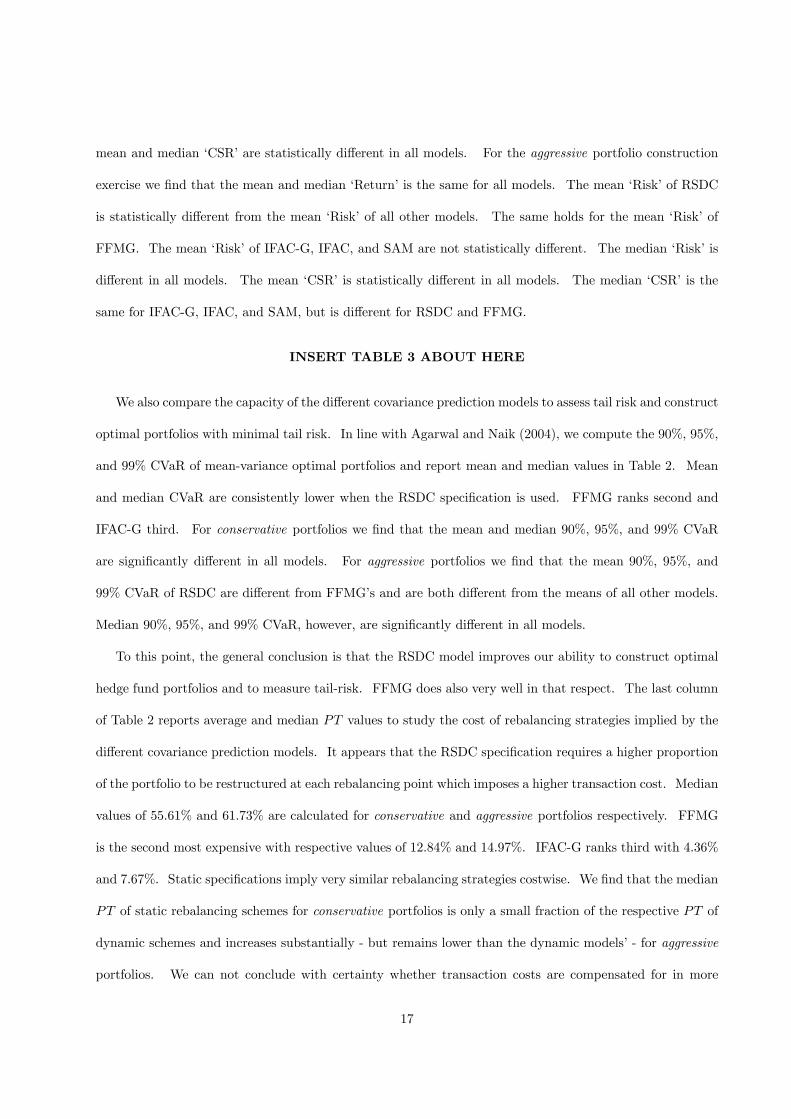
To this point, the general conclusion is that the RSDC model improves our ability to construct optimal

hedge fund portfolios and to measure tail-risk. FFMG does also very well in that respect. The last column

of Table 2 reports average and median PT values to study the cost of rebalancing strategies implied by the

different covariance prediction models. It appears that the RSDC specification requires a higher proportion

of the portfolio to be restructured at each rebalancing point which imposes a higher transaction cost. Median

values of 55.61% and 61.73% are calculated for conservative and aggressive portfolios respectively. FFMG

is the second most expensive with respective values of 12.84% and 14.97%. IFAC-G ranks third with 4.36%

and 7.67%. Static specifications imply very similar rebalancing strategies costwise. We find that the median

PT of static rebalancing schemes for conservative portfolios is only a small fraction of the respective PT of

dynamic schemes and increases substantially - but remains lower than the dynamic models’ - for aggressive

portfolios. We can not conclude with certainty whether transaction costs are compensated for in more

17

variable weighting strategies since the actual transaction cost is not easy to estimate in the case of hedge

funds and funds of funds. Moreover transaction costs may vary with the ‘buyer’, i.e. size of a fund of funds,

and the ‘seller’, i.e. liquid vs. less liquid strategies, which makes it even more difficult to create a uniform

decision rule.

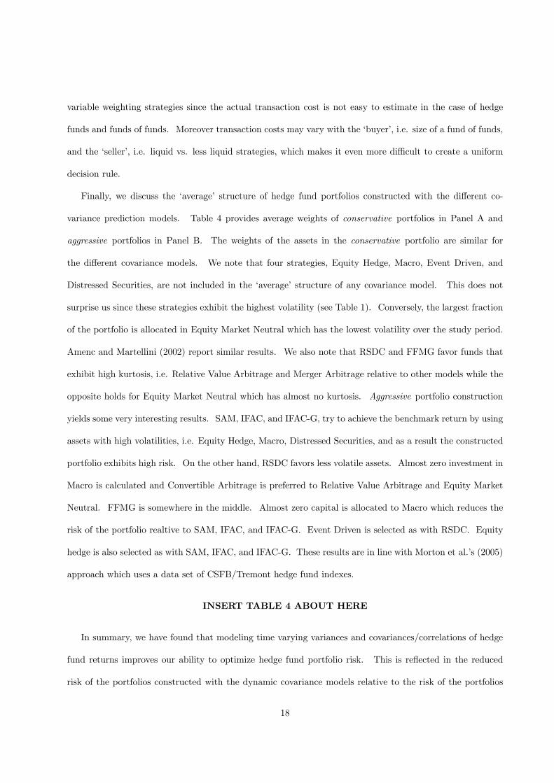
Finally, we discuss the ‘average’ structure of hedge fund portfolios constructed with the different co-

variance prediction models. Table 4 provides average weights of conservative portfolios in Panel A and

aggressive portfolios in Panel B. The weights of the assets in the conservative portfolio are similar for

the different covariance models. We note that four strategies, Equity Hedge, Macro, Event Driven, and

Distressed Securities, are not included in the ‘average’ structure of any covariance model. This does not

surprise us since these strategies exhibit the highest volatility (see Table 1). Conversely, the largest fraction

of the portfolio is allocated in Equity Market Neutral which has the lowest volatility over the study period.

Amenc and Martellini (2002) report similar results. We also note that RSDC and FFMG favor funds that

exhibit high kurtosis, i.e. Relative Value Arbitrage and Merger Arbitrage relative to other models while the

opposite holds for Equity Market Neutral which has almost no kurtosis. Aggressive portfolio construction

yields some very interesting results. SAM, IFAC, and IFAC-G, try to achieve the benchmark return by using

assets with high volatilities, i.e. Equity Hedge, Macro, Distressed Securities, and as a result the constructed

portfolio exhibits high risk. On the other hand, RSDC favors less volatile assets. Almost zero investment in

Macro is calculated and Convertible Arbitrage is preferred to Relative Value Arbitrage and Equity Market

Neutral. FFMG is somewhere in the middle. Almost zero capital is allocated to Macro which reduces the

risk of the portfolio realtive to SAM, IFAC, and IFAC-G. Event Driven is selected as with RSDC. Equity

hedge is also selected as with SAM, IFAC, and IFAC-G. These results are in line with Morton et al.’s (2005)

approach which uses a data set of CSFB/Tremont hedge fund indexes.

INSERT TABLE 4 ABOUT HERE

In summary, we have found that modeling time varying variances and covariances/correlations of hedge

fund returns improves our ability to optimize hedge fund portfolio risk. This is reflected in the reduced

risk of the portfolios constructed with the dynamic covariance models relative to the risk of the portfolios

18

constructed with the other models. It is also reflected in the portfolio ‘CSR’, which ranks RSDC first, FFMG

second, and IFAC-G, IFAC, and SAM, third, fourth, and fifth respectively. The difference in the mean and

median ‘CSR’ is almost always significant at the 5% level. In addition, we have shown that the RSDC

covariance model improves our ability in risk measurement and confirmed that this result is statistically

significant. The overall ranking of covariance models in terms of risk measurement resembles the ‘CSR’

ranking. We have found, however, that RSDC imposes a substantially more variable weighting strategy

than other models. FFMG also requires variable rebalancing but its cost is closer to that imposed by the

other covariance models. IFAC-G’s cost of rebalancing is even closer to the static models’.

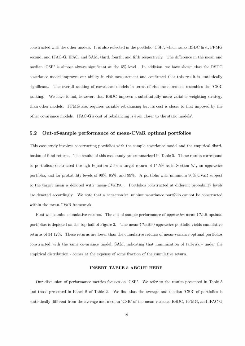
5.2 Out-of-sample performance of mean-CVaR optimal portfolios

This case study involves constructing portfolios with the sample covariance model and the empirical distri-

bution of fund returns. The results of this case study are summarized in Table 5. These results correspond

to portfolios constructed through Equation 2 for a target return of 15.5% as in Section 5.1, an aggressive

portfolio, and for probability levels of 90%, 95%, and 99%. A portfolio with minimum 90% CVaR subject

to the target mean is denoted with ‘mean-CVaR90’. Portfolios constructed at different probability levels

are denoted accordingly. We note that a conservative, minimum-variance portfolio cannot be constructed

within the mean-CVaR framework.

First we examine cumulative returns. The out-of-sample performance of aggressive mean-CVaR optimal

portfolios is depicted on the top half of Figure 2. The mean-CVaR90 aggressive portfolio yields cumulative

returns of 34.12%. These returns are lower than the cumulative returns of mean-variance optimal portfolios

constructed with the same covariance model, SAM, indicating that minimization of tail-risk - under the

empirical distribution - comes at the expense of some fraction of the cumulative return.

INSERT TABLE 5 ABOUT HERE

Our discussion of performance metrics focuses on ‘CSR’. We refer to the results presented in Table 5

and those presented in Panel B of Table 2. We find that the average and median ‘CSR’ of portfolios is

statistically different from the average and median ‘CSR’ of the mean-variance RSDC, FFMG, and IFAC-G

19

portfolios. Also, the average and median ‘CSR’ of mean-CVaR95 portfolios is statistically different from

the average and median ‘CSR’ of the mean-variance RSDC, FFMG, and IFAC-G, IFAC, and SAM portfolios

but not different from the mean and median ‘CSR’ of mean-CVaR90 portfolios. Finally, the average and

median ‘CSR’ of mean-CVaR99 portfolios is statistically different from the average and median ‘CSR’ of the

mean-variance RSDC, FFMG, and IFAC-G, IFAC, and SAM portfolios and mean-CVaR90, mean-CVaR95

portfolios.

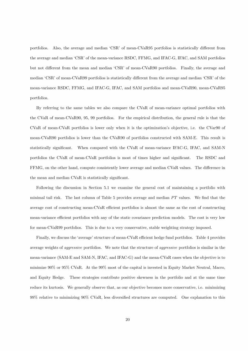
By referring to the same tables we also compare the CVaR of mean-variance optimal portfolios with

the CVaR of mean-CVaR90, 95, 99 portfolios. For the empirical distribution, the general rule is that the

CVaR of mean-CVaR portfolios is lower only when it is the optimization’s objective, i.e. the CVar90 of

mean-CVaR90 portfolios is lower than the CVaR90 of portfolios constructed with SAM-E. This result is

statistically significant. When compared with the CVaR of mean-variance IFAC-G, IFAC, and SAM-N

portfolios the CVaR of mean-CVaR portfolios is most of times higher and significant. The RSDC and

FFMG, on the other hand, compute consistently lower average and median CVaR values. The difference in

the mean and median CVaR is statistically significant.

Following the discussion in Section 5.1 we examine the general cost of maintaining a portfolio with

minimal tail risk. The last column of Table 5 provides average and median PT values. We find that the

average cost of constructing mean-CVaR efficient portfolios is almost the same as the cost of constructing

mean-variance efficient portfolios with any of the static covariance prediction models. The cost is very low

for mean-CVaR99 portfolios. This is due to a very conservative, stable weighting strategy imposed.

Finally, we discuss the ‘average’ structure of mean-CVaR efficient hedge fund portfolios. Table 4 provides

average weights of aggressive portfolios. We note that the structure of aggressive portfolios is similar in the

mean-variance (SAM-E and SAM-N, IFAC, and IFAC-G) and the mean-CVaR cases when the objective is to

minimize 90% or 95% CVaR. At the 99% most of the capital is invested in Equity Market Neutral, Macro,

and Equity Hedge. These strategies contribute positive skewness in the portfolio and at the same time

reduce its kurtosis. We generally observe that, as our objective becomes more conservative, i.e. minimizing

99% relative to minimizing 90% CVaR, less diversified structures are computed. One explanation to this

20

feature can be the following. The mean-CVaR algorithm seeks minimal tail risk portfolios or equivalently,

portfolios exhibiting minimal kurtosis. As a result, the more conservative the objective becomes, the more

likely it is that assets exhibiting high kurtosis are excluded and assets exhibiting low kurtosis are included

in the portfolio.

In summary, we have shown that the cumulative returns of mean-CVaR optimal portfolios are generally

lower than the cumulative returns of mean-variance optimal portfolios. We have also shown that mean and

median ‘CSR’ of mean-CVaR optimal portfolios are lower than mean and median ‘CSR’ of mean-variance

optimal portfolios and that this difference is most of the times statistically significant at the 5% level.

Also, the CVaR of mean-CVaR optimal portfolios is only lower than the CVaR of mean-variance portfolios

constructed with the SAM-E model. We have found that the cost of maintaining a mean-CVaR optimal

portfolio is similar on average with the cost of maintaining a mean-variance (constructed with the SAM

and IFAC covariance models) efficient portfolio with the same benchmark return. Finally, we have found

similar allocations between mean-CVaR and mean-variance (SAM, IFAC, and IFAC-G) efficient portfolios.

The portfolio structure changes significantly for more conservative structures i.e. mean-CVaR99 portfolios,

where the largest fraction of the portfolio is invested in assets exhibiting low kurtosis.

5.3 Additional results

In additional, unreported work (available from the authors upon request) we have extended our analysis to

incorporate: (a) one additional target return, 14.5%, (b) one alternative rebalancing frequency, 3 months,

(c) one shorter estimation period, 120 months, and one longer estimation period, 168 months, 2 years apart

each from the 144 months period used in the experiments reported in the previous sections, (d) returns in

the excess of the risk free rate4 as opposed to absolute returns used in the reported results. In addition we

have performed our experiments under various combinations of the latter.

The study of mean-variance and mean-CVaR optimal portfolios targeting annual expected return of 14.5%

neither offers any additional evidence nor it contradicts any of the conclusions that drawn in this analysis.

In fact, the results are veryy similar with those presented for the benchmark return 15.5%.4We use the 3-month US Treasury-bill as a proxy for the risk free rate.

21

The findings for the three months rebalancing are summarized as follows. For conservative portfolios

the cumulative return of the RSDC model is 20.46%, the FFMG model is 15.81%, the IFAC-G 13.70%, the

IFAC 13.64%, and the SAM-E and SAM-N 13.30%. These are lower than the cumulative returns achieved

with the respective models and 1-month rebalancing. The mean and median CSR of the RSDC are 1.44

and 1.06 respectively. The FFMG mean and median CSR are 1.07 and 1.10 respectively. These values are

not statistically different but they are different - and higher - from the respective figures of IFAC-G, IFAC,

and SAM portfolios. These are also the conclusions drawn in Section 5.1.

The use of longer/shorter estimation periods and/or excess returns also does not alter our conclusions.

For example, in the case that the first 120 months of excess returns are used to estimate the different

covariance models, and aggressive portfolios are constructed with monthly rebalancing. The cumulative

excess returns rank RSDC first with 38.18%, FFMG second with 36.22%, IFAC, SAM, and IFAC-G, with

35.14%, 34.94%, and 34.93% respectively. The ‘CSR’ ranks RSDC first with statistically different mean and

median with all other models.

In summary, we examined if certain preferences in our investment exercise, i.e. target returns, frequency

of rebalancing, size of the estimation period, excess returns, have an impact in the conclusions of Sections

5.1 and 5.2. We have found that the notion of our results remains unchanged.

6 Conclusion

Despite the facts that hedge funds are dynamic investments, the variance and covariance of most financial

time series - the funds’ underlying assets - are time-varying, the time series of fund returns exhibit volatility

clustering and high kurtosis, to date studies do not account for possible time-variance of the variances and

covariances/correlations of hedge fund returns.

This article addresses the issue of time-varying variances and covariances/correlations of hedge fund

returns and concentrate on the potential impacts in terms of hedge fund portfolio construction and risk

measurement. We compare the performance of different methods of forecasting variances and covari-

ances/correlations and judge which model improves our ability to construct optimal hedge fund portfolios

22

and measure tail-risk.

We find that a regime switching dynamic correlations model, RSDC, reduces portfolio risk and improves

the out-of-sample risk-adjusted realized returns. We also find that the CVaR of the portfolio constructed

with the RSDC model is the lowest among alternative covariance models. This suggests that the RSDC

covariance model represents a more accurate tool for tail-risk measurement. These results are statistically

significant. The full-factor multivariate GARCH model, FFMG ranks second with significant differences.

The implicit factor GARCH, implicit factor, and sample covariance models rank third, fourth, and fifth with

average and median metrics’ values that in most cases are not statistically different. When we study the cost

of rebalancing we find that the RSDC imposes substantially higher transaction costs than the FFMG which

is the second most variable weighting strategy. Changing various preferences in our investment exercise,

i.e. portfolio rebalancing period, estimation period, did not alter the overall verdict that the RSDC and

the FFMG models provide a superior tool for portfolio choice and risk measurement among the considered

methodologies.

Acknowledgements

The authors thank the two referees for their detailed and constructive advice. We also thank Elias

Tzavalis for his comments and advice, Anca Dimitriu, George Leledakis, Loukia Meligkotsidou, George

Skiadopoulos for their suggestions, and Dimitris Alexopoulos, George Chalamandaris, Dimitris Flamouris,

Manolis Liodakis, Vassilios Siokis, Michael Steliaros, for helpful discussions on practical issues. A previous

version of this paper was presented in 2005 at the Quant Congress USA, International Summer School in

Risk Measurement and Control, 12th Annual Conference of the Multinational Finance Society, and the 2nd

Advances in Financial Forecasting International Symposium. We thank participants at these meetings for

their comments.

23

References

[1] Ackermann, C., R. McEnally, and D. Ravenscraft, 1999, The performance of hedge funds: Risk, return,

and incentives, Journal of Finance, 54, 833-874.

[2] Agarwal, V. and N.Y. Naik, 2004, Risks and portfolio decisions involving hedge funds, Review of Financial

Studies, 17, 1, 63-98.

[3] Alexander, C., 2001, Orthogonal GARCH, in C. Alexander (ed.) Mastering Risk, 2, Financial Times-

Prentice Hall, 21-38.

[4] Alexander, C. and A. Dimitiu, 2005, Detecting switching strategies in equity hedge funds returns, Journal

of Alternative investments, 8, 1, 7-13.

[5] Alexander, C. and A. Dimitriu, 2004, The art of investing in hedge funds: Fund selection and optimal

allocation, Working paper, ICMA Centre, University of Reading.

[6] Amenc, N. and L. Martellini, 2002, Portfolio optimization and hedge fund style allocation decisions,

Journal of Alternative Investments, 5, 7-20.

[7] Amin, G. S. and H. M. Kat, 2003, Stocks, bonds, and hedge funds: Not a free lunch, Journal of Portfolio

Management, 2, 113-120.

[8] Barès, P.-A., R. Gibson, and S. Gyger, 2002, Hedge fund allocation with survival uncertainty and invest-

ment constraints, Working paper, Swiss Federal Institute of Technology.

[9] Brown, S.J., W.N. Goetzmann, and R.G. Ibbotson, 1999, Offshore hedge funds: Survival and performance

1989-1995, Journal of Business, 72, 91-118.

[10] Chambers, R. G. and J. Quiggin, 2005, Linear-risk-tolerant, invariant risk preferences, Economics Let-

ters, forthcoming.

[11] Chan, L.K.C., J. Karceski, and J. Lakonishok, 1999, On portfolio optimization: Forecasting covariances

and choosing the risk model, Review of Financial Studies, 12, 5, 937-974.

24

[12] Chan, N, M. Getmansky, S.M. Haas, and A.W. Lo, 2005, Systemic risk and hedge funds, NBER working

paper.

[13] Cvitanic, J., A. Lazrak, L. Martellini, and F. Zapatero, 2003, Optimal allocation to hedge funds: An

empirical analysis, Quantitative Finance, 3, 1-12.

[14] Davies, R.J., Kat, H. and Lu, S., 2005, Fund of hedge funds portfolio selection: A multiple-objective

approach, Working paper, SSRN.

[15] Duarte, A.M., 1999, Fast computation of efficient portfolios, Journal of Risk, 1, 71-94.

[16] Edwards, F.R. and M.O. Caglayan, 2001, Hedge fund performance and manager skill, Journal of Futures

Markets, 21, 11, 1002-1028.

[17] Engle, R. F., 2002, Dynamic conditional correlation: A simple class of multivariate GARCH models,

Journal of Business and Economic Statistics, 20, 339-350.

[18] Ferry, J., 2004, The index link, RISK, September, 20-21.

[19] Fung, W., and D. A. Hsieh, 1997, Empirical characteristics of dynamic trading strategies: The case of

hedge funds, Review of Financial Studies, 10, 275-302.

[20] Getmansky, M., A.W. Lo, and I. Makarov, 2004, An econometric model of serial correlation and illiq-

uidity in hedge fund returns, Journal of Financial Economics, 74, 529-609.

[21] Greyserman, A. D.H. Jones, and W.E. Strawderman, 2005, Portfolio selection using hierarchical

Bayesian analysis and MCMC methods, Journal of Banking and Finance, forthcoming.

[22] Hagelin, N. and B. Pramborg, 2003, Evaluating gains from diversifying into hedge funds using dynamic

investment strategies, in: B. Schachter, Intelligent hedge fund investing (Risk Waters Group, London).

[23] Kat, H.M., 2004, In search of the optimal fund of hedge funds, Journal of Wealth Management, 6, 4,

43-51.

25

[24] Krokhmal, P., S. Uryasev, and G. Zrazhevsky, 2002, Risk management for hedge fund portfolios: A

comparative analysis of linear portfolio rebalancing strategies, Journal of Alternative Investments, 5, 1,

10-29.

[25] Ledoit, O. and M. Wolf, 2003, Improved estimation of the covariance matrix of stock returns with an

application to portfolio selection, Journal of Empirical Finance, 10, 603-621.

[26] Liew, J., 2003, Hedge fund index investing examined, Journal of Portfolio Management, 29, 2, 113-123.

[27] Markowitz, H.M., 1952, Portfolio selection, Journal of Finance, 7, 77-91.

[28] McFall Lamm, R., 2003, Asymmetric returns and optimal hedge fund portfolios, Journal of Alternative

Investments, 6, 2, 9-21.

[29] Morton, D. P., E. Popova, and I. Popova, 2005, Efficient fund of hedge funds construction under

downside risk measures, Journal of Banking and Finance, forthcoming.

[30] Pelletier, D., 2005, Regime switching for dynamic correlations, Journal of Econometrics, forthcoming.

[31] Popova, I., D.P. Morton, and E. Popova, 2003, Optimal hedge fund allocation with asymmetric prefer-

ences and distributions, Working paper, University of Texas at Austin

[32] Rockafellar, R.T. and S. Uryasev, 2002, Conditional value-at-risk for general loss distributions, Journal

of Banking and Finance, 26, 1443-1471.

[33] Rockafellar, R.T. and S. Uryasev, 2000, Optimization of Conditional Value-At-Risk, Journal of Risk, 2,

3, 21-41.

[34] Rockafellar, R.T., S. Uryasev, and M. Zabarankin, 2005, Portfolio analysis with general deviation mea-

sures, Journal of Banking and Finance, forthcoming.

[35] Terhaar, K., R. Staub, and B. Singer, 2003, Appropriate policy allocation for alternative investments,

Journal of Portfolio Management, 29, 3, 101-111.

26

[36] Vrontos, I.D., P. Dellaportas, and D.N. Politis, 2003, A full-factor multivariate GARCH model, Econo-

metrics Journal, 6, 312-334.

[37] Walker, D. and J. Butcher, 2004, Passive investing gets active, RISK, September, 22-29.

[38] Zivot, E. and J. Wang, Modeling Financial Time Series with S-PLUS, Springer-Verlag, October 2002.

27

A Tables and Figures

28

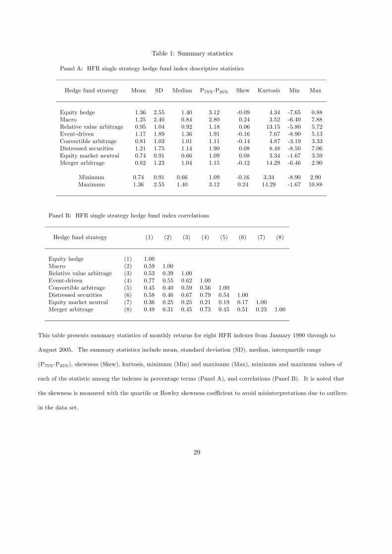
Table 1: Summary statistics

Panel A: HFR single strategy hedge fund index descriptive statistics

Hedge fund strategy Mean SD Median P75%-P25% Skew Kurtosis Min Max

Equity hedge 1.36 2.55 1.40 3.12 -0.09 4.34 -7.65 0.88Macro 1.25 2.40 0.84 2.80 0.24 3.52 -6.40 7.88Relative value arbitrage 0.95 1.04 0.92 1.18 0.06 13.15 -5.80 5.72Event-driven 1.17 1.89 1.36 1.91 -0.16 7.67 -8.90 5.13Convertible arbitrage 0.81 1.03 1.01 1.11 -0.14 4.87 -3.19 3.33Distressed securities 1.21 1.75 1.14 1.90 0.08 8.48 -8.50 7.06Equity market neutral 0.74 0.91 0.66 1.09 0.08 3.34 -1.67 3.59Merger arbitrage 0.82 1.23 1.04 1.15 -0.12 14.29 -6.46 2.90

Minimum 0.74 0.91 0.66 1.09 -0.16 3.34 -8.90 2.90Maximum 1.36 2.55 1.40 3.12 0.24 14.29 -1.67 10.88

Panel B: HFR single strategy hedge fund index correlations

Hedge fund strategy (1) (2) (3) (4) (5) (6) (7) (8)

Equity hedge (1) 1.00Macro (2) 0.59 1.00Relative value arbitrage (3) 0.53 0.39 1.00Event-driven (4) 0.77 0.55 0.62 1.00Convertible arbitrage (5) 0.45 0.40 0.59 0.56 1.00Distressed securities (6) 0.58 0.46 0.67 0.79 0.54 1.00Equity market neutral (7) 0.36 0.25 0.25 0.21 0.19 0.17 1.00Merger arbitrage (8) 0.49 0.31 0.45 0.73 0.45 0.51 0.23 1.00

This table presents summary statistics of monthly returns for eight HFR indexes from January 1990 through to

August 2005. The summary statistics include mean, standard deviation (SD), median, interquartile range

(P75%-P25%), skewness (Skew), kurtosis, minimum (Min) and maximum (Max), minimum and maximum values of

each of the statistic among the indexes in percentage terms (Panel A), and correlations (Panel B). It is noted that

the skewness is measured with the quartile or Bowley skewness coefficient to avoid misinterpretations due to outliers

in the data set.

29

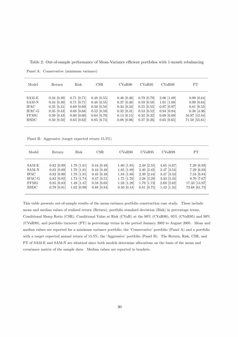
Table 2: Out-of-sample performance of Mean-Variance efficient portfolios with 1-month rebalancing

Panel A: Conservative (minimum variance)

Model Return Risk CSR CVaR90 CVaR95 CVaR99 PT

SAM-E 0.34 [0.39] 0.71 [0.71] 0.48 [0.55] 0.46 [0.46] 0.79 [0.79] 2.06 [1.89] 0.99 [0.64]SAM-N 0.34 [0.39] 0.71 [0.71] 0.48 [0.55] 0.37 [0.36] 0.59 [0.58] 1.01 [1.00] 0.99 [0.64]IFAC 0.35 [0.41] 0.69 [0.69] 0.50 [0.58] 0.34 [0.34] 0.55 [0.55] 0.97 [0.97] 0.81 [0.55]IFAC-G 0.35 [0.43] 0.68 [0.68] 0.52 [0.59] 0.32 [0.31] 0.53 [0.52] 0.94 [0.94] 6.38 [4.36]FFMG 0.39 [0.43] 0.60 [0.60] 0.64 [0.70] 0.14 [0.15] 0.32 [0.32] 0.69 [0.69] 16.97 [12.84]RSDC 0.50 [0.50] 0.63 [0.62] 0.85 [0.74] 0.08 [0.06] 0.27 [0.26] 0.65 [0.65] 71.50 [55.61]

Panel B: Aggressive (target expected return 15.5%)

Model Return Risk CSR CVaR90 CVaR95 CVaR99 PT

SAM-E 0.82 [0.89] 1.79 [1.81] 0.44 [0.48] 1.80 [1.85] 2.49 [2.55] 4.85 [4.67] 7.29 [6.93]SAM-N 0.82 [0.89] 1.79 [1.81] 0.44 [0.48] 1.85 [1.89] 2.40 [2.45] 3.47 [3.54] 7.29 [6.93]IFAC 0.82 [0.90] 1.78 [1.81] 0.45 [0.48] 1.84 [1.88] 2.39 [2.44] 3.47 [3.53] 7.34 [6.84]IFAC-G 0.82 [0.92] 1.73 [1.74] 0.47 [0.51] 1.75 [1.76] 2.28 [2.29] 3.33 [3.34] 9.70 [7.67]FFMG 0.85 [0.83] 1.49 [1.47] 0.58 [0.65] 1.33 [1.28] 1.79 [1.73] 2.69 [2.62] 17.33 [14.97]RSDC 0.79 [0.81] 1.02 [0.99] 0.88 [0.84] 0.50 [0.44] 0.81 [0.75] 1.43 [1.34] 73.68 [61.73]

This table presents out-of-sample results of the mean-variance portfolio construction case study. These include

mean and median values of realized return (Return), portfolio standard deviation (Risk) in percentage terms,

Conditional Sharp Ratio (CSR), Conditional Value at Risk (CVaR) at the 90% (CVaR90), 95% (CVaR95) and 99%

(CVaR99), and portfolio turnover (PT) in percentage terms in the period January 2002 to August 2005. Mean and

median values are reported for a minimum variance portfolio, the ‘Conservative’ portfolio (Panel A) and a portfolio

with a target expected annual return of 15.5%, the ‘Aggressive’ portfolio (Panel B). The Return, Risk, CSR, and

PT of SAM-E and SAM-N are identical since both models determine allocations on the basis of the mean and

covariance matrix of the sample data. Median values are reported in brackets.

30

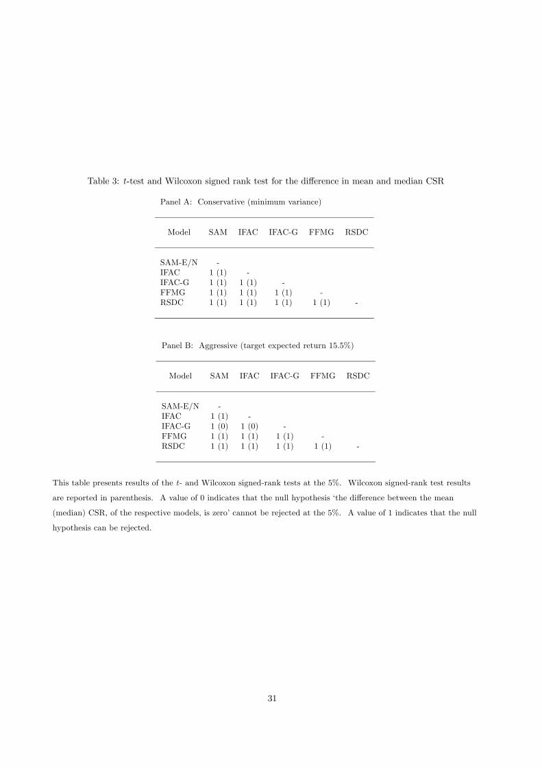
Table 3: t-test and Wilcoxon signed rank test for the difference in mean and median CSR

Panel A: Conservative (minimum variance)

Model SAM IFAC IFAC-G FFMG RSDC

SAM-E/N -IFAC 1 (1) -IFAC-G 1 (1) 1 (1) -FFMG 1 (1) 1 (1) 1 (1) -RSDC 1 (1) 1 (1) 1 (1) 1 (1) -

Panel B: Aggressive (target expected return 15.5%)

Model SAM IFAC IFAC-G FFMG RSDC

SAM-E/N -IFAC 1 (1) -IFAC-G 1 (0) 1 (0) -FFMG 1 (1) 1 (1) 1 (1) -RSDC 1 (1) 1 (1) 1 (1) 1 (1) -

This table presents results of the t- and Wilcoxon signed-rank tests at the 5%. Wilcoxon signed-rank test results

are reported in parenthesis. A value of 0 indicates that the null hypothesis ‘the difference between the mean

(median) CSR, of the respective models, is zero’ cannot be rejected at the 5%. A value of 1 indicates that the null

hypothesis can be rejected.

31

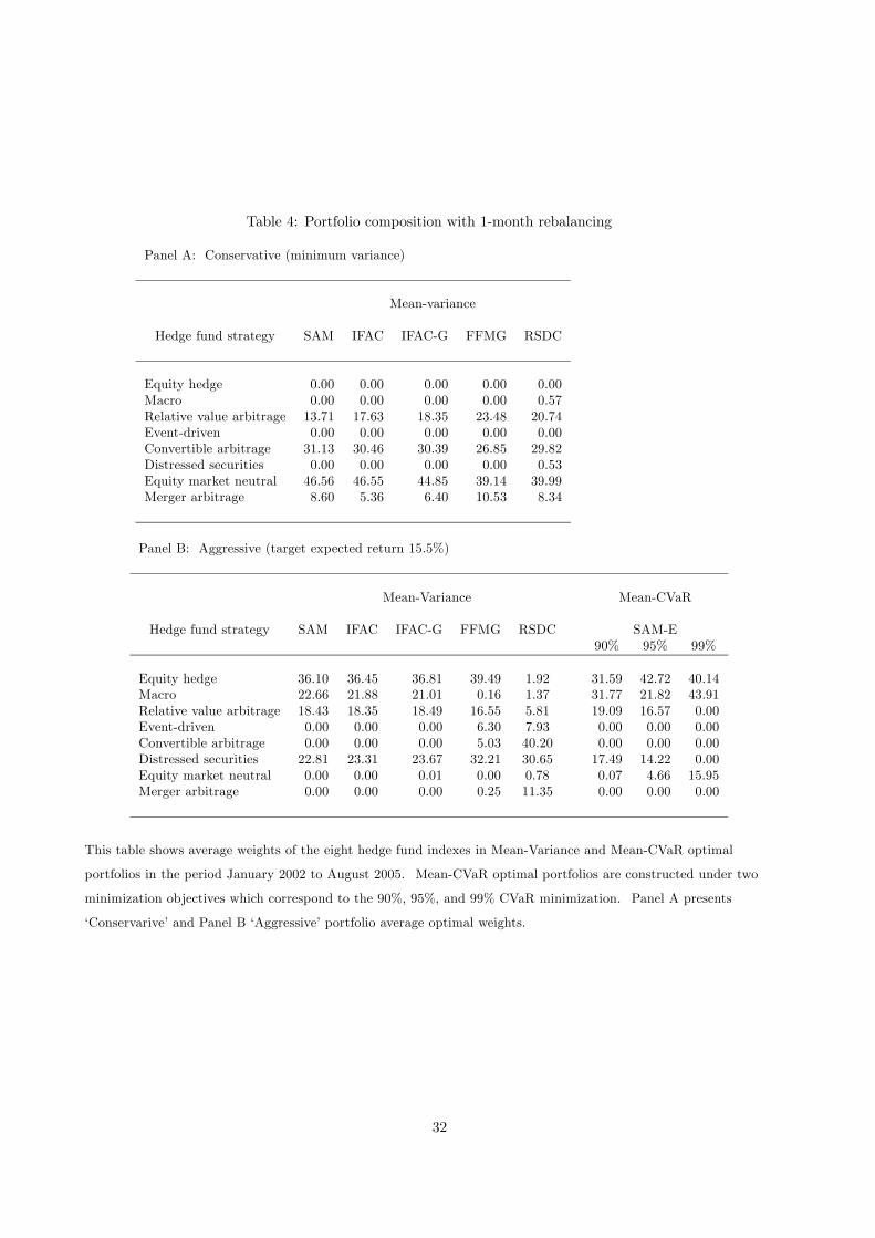
Table 4: Portfolio composition with 1-month rebalancing

Panel A: Conservative (minimum variance)

Mean-variance

Hedge fund strategy SAM IFAC IFAC-G FFMG RSDC

Equity hedge 0.00 0.00 0.00 0.00 0.00Macro 0.00 0.00 0.00 0.00 0.57Relative value arbitrage 13.71 17.63 18.35 23.48 20.74Event-driven 0.00 0.00 0.00 0.00 0.00Convertible arbitrage 31.13 30.46 30.39 26.85 29.82Distressed securities 0.00 0.00 0.00 0.00 0.53Equity market neutral 46.56 46.55 44.85 39.14 39.99Merger arbitrage 8.60 5.36 6.40 10.53 8.34

Panel B: Aggressive (target expected return 15.5%)

Mean-Variance Mean-CVaR

Hedge fund strategy SAM IFAC IFAC-G FFMG RSDC SAM-E90% 95% 99%

Equity hedge 36.10 36.45 36.81 39.49 1.92 31.59 42.72 40.14Macro 22.66 21.88 21.01 0.16 1.37 31.77 21.82 43.91Relative value arbitrage 18.43 18.35 18.49 16.55 5.81 19.09 16.57 0.00Event-driven 0.00 0.00 0.00 6.30 7.93 0.00 0.00 0.00Convertible arbitrage 0.00 0.00 0.00 5.03 40.20 0.00 0.00 0.00Distressed securities 22.81 23.31 23.67 32.21 30.65 17.49 14.22 0.00Equity market neutral 0.00 0.00 0.01 0.00 0.78 0.07 4.66 15.95Merger arbitrage 0.00 0.00 0.00 0.25 11.35 0.00 0.00 0.00

This table shows average weights of the eight hedge fund indexes in Mean-Variance and Mean-CVaR optimal

portfolios in the period January 2002 to August 2005. Mean-CVaR optimal portfolios are constructed under two

minimization objectives which correspond to the 90%, 95%, and 99% CVaR minimization. Panel A presents

‘Conservarive’ and Panel B ‘Aggressive’ portfolio average optimal weights.

32

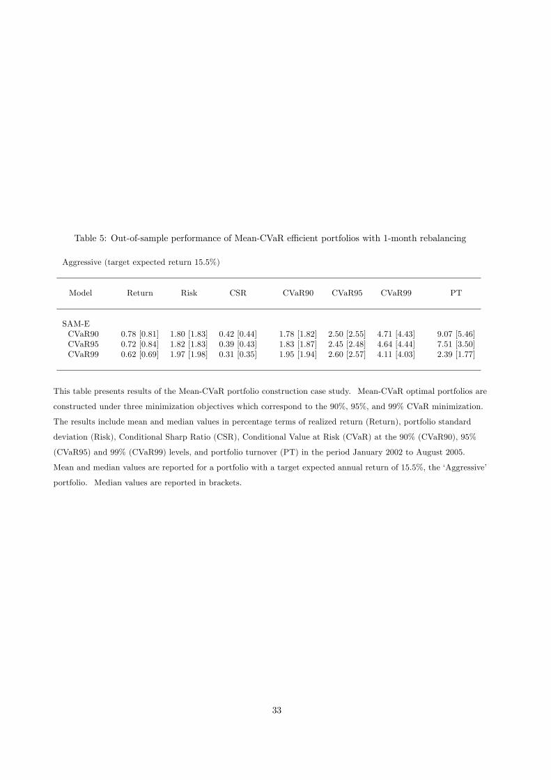
Table 5: Out-of-sample performance of Mean-CVaR efficient portfolios with 1-month rebalancing

Aggressive (target expected return 15.5%)

Model Return Risk CSR CVaR90 CVaR95 CVaR99 PT

SAM-ECVaR90 0.78 [0.81] 1.80 [1.83] 0.42 [0.44] 1.78 [1.82] 2.50 [2.55] 4.71 [4.43] 9.07 [5.46]CVaR95 0.72 [0.84] 1.82 [1.83] 0.39 [0.43] 1.83 [1.87] 2.45 [2.48] 4.64 [4.44] 7.51 [3.50]CVaR99 0.62 [0.69] 1.97 [1.98] 0.31 [0.35] 1.95 [1.94] 2.60 [2.57] 4.11 [4.03] 2.39 [1.77]

This table presents results of the Mean-CVaR portfolio construction case study. Mean-CVaR optimal portfolios are

constructed under three minimization objectives which correspond to the 90%, 95%, and 99% CVaR minimization.

The results include mean and median values in percentage terms of realized return (Return), portfolio standard

deviation (Risk), Conditional Sharp Ratio (CSR), Conditional Value at Risk (CVaR) at the 90% (CVaR90), 95%

(CVaR95) and 99% (CVaR99) levels, and portfolio turnover (PT) in the period January 2002 to August 2005.

Mean and median values are reported for a portfolio with a target expected annual return of 15.5%, the ‘Aggressive’

portfolio. Median values are reported in brackets.

33

2000 2001 2002 2003 2004 2005

0.42

0.44

0.46

0.48

0.5

0.52

0.54EH - CA

2000 2001 2002 2003 2004 20050.3

0.32

0.34

0.36

0.38

0.4

0.42

EH - EMN

2000 2001 2002 2003 2004 20050.38

0.4

0.42

0.44

0.46

0.48

0.5EH - MA

2000 2001 2002 2003 2004 20050.66

0.68

0.7

0.72

RVA - DS

2000 2001 2002 2003 2004 20050.16

0.18

0.2

0.22

0.24

0.26RVA - EMN

2000 2001 2002 2003 2004 20050.38

0.4

0.42

0.44

0.46

RVA - MA

2000 2001 2002 2003 2004 2005

0.56

0.58

0.6

0.62

0.64

0.66

0.68ED - CA

2000 2001 2002 2003 2004 20050.16

0.18

0.2

0.22

0.24

0.26ED - EMN

2000 2001 2002 2003 2004 2005

0.16

0.18

0.2

0.22

0.24DS - EMN

Figure 1: Correlation coefficients for selected pairs including the Equity hedge (EH), Relative value arbitrage

(RVA), Event driven (ED), Convertible arbitrage (CA), Distressed securities (DS), Equity market neutral

(EMN), and the Merger arbitrage (MA) hedge fund indexes. The first point of each series corresponds

to the respective correlation during January 1990 to December 1999. Subsequent points are computed by

sequentially adding index returns in the intial sample.

34

2002 2003 2004 2005

0

0.05

0.1

0.15

0.2

0.25

0.3

0.35

0.4Conservative

Cum

mul

ativ

e R

etur

ns

SAM-E/NIFACIFACGFFMGRSDC

2002 2003 2004 2005

0

0.05

0.1

0.15

0.2

0.25

0.3

0.35

0.4Aggressive

SAM-E/NIFACIFACGFFMGRSDCMCVaR90MCVAR95MCVaR99

2002 2003 2004 2005

0.005

0.01

0.015

0.02

Conservative

Sta

ndar

d D

evia

tion

2002 2003 2004 2005

0.005

0.01

0.015

0.02

Aggressive

Figure 2: Cumulative returns of ‘Conservative’ and ‘Aggressive’ portfolios in the out-of-sample period Jan-

uary 2002 to August 2005 are presented on the top half. The bottom half presents the respective portfolio

standard deviation.

35