Embed Size (px)
Citation preview
Hedging and Value-at-Risk(VaR)
Single asset VaR Delta-VaR for portfoliosDelta-Gamma VaRsimulated VaR
Finance 70520, Spring 2002Risk Management & Financial EngineeringS. MannThe Neeley School
Run
Value at Risk (VaR)
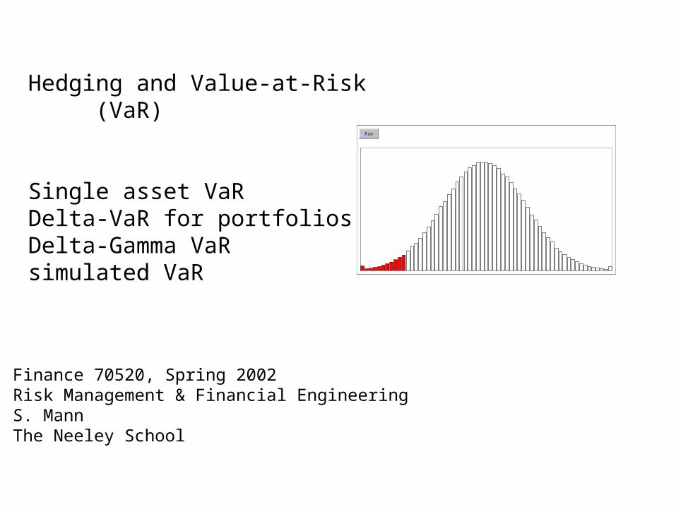
“VaR measures the worst expected loss over a given time intervalunder normal market conditions at a given confidence level.”
- Jorion (1997)
“Value at Risk is an estimate, with a given degree of confidence, of how much one can lose from one’s portfolio over a given time horizon.”
- Wilmott (1998)
“Value-at-Risk or VAR is a dollar measure of the minimum loss that would be expected over a period of time with a given probability”
- Chance(1998)
95% confidence level VaR 5% probability minimum loss (over given horizon)
max. loss with 95% confidence min.loss with 5% probability (for given time interval)
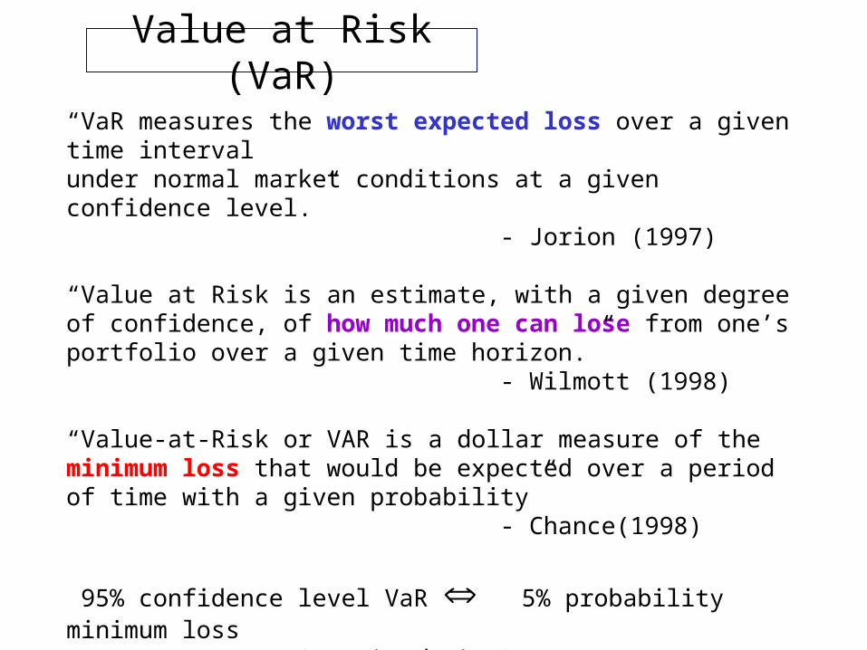
Asset price standard deviation
Assume lognormal returns: Let dS/S ~ lognormal() where is annualized return volatility (standard deviation)
The standard deviation of the asset price (S) over a period is:
S ( .5) = S For example, let
S = $ 100.00 = 40% = 1 week = 1/52
then the weekly standard deviation (s.d.) of the price is
weekly s.d. = 100 (0.40) (.192).5 = 40(0.139) = $ 5.55
similarly, daily s.d. = 100(0.40)(1/252).5 = 40(0.063) = $ 2.52
monthly s.d. = 0.40(0.40)(1/12).5 = 40(0.289) = $ 11.55
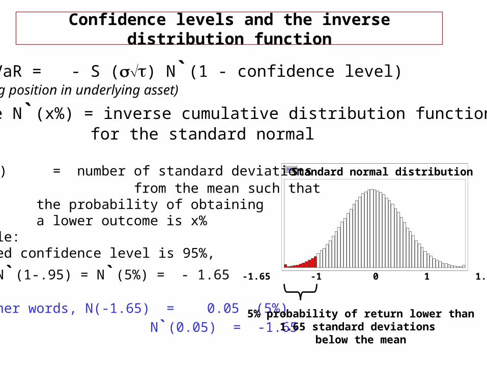
Confidence levels and the inverse distribution function
Let VaR = - S () N`(1 - confidence level)(for long position in underlying asset)
where N`(x%) = inverse cumulative distribution function for the standard normal
Run N`(x%) = number of standard deviations from the mean such that
the probability of obtaining a lower outcome is x%
example:desired confidence level is 95%,
then N`(1-.95) = N`(5%) = - 1.65
In other words, N(-1.65) = 0.05 (5%)
so N`(0.05) = -1.65 5% probability of return lower than
1.65 standard deviations below the mean
-1.65 -1 0 1 1.65
Standard normal distribution
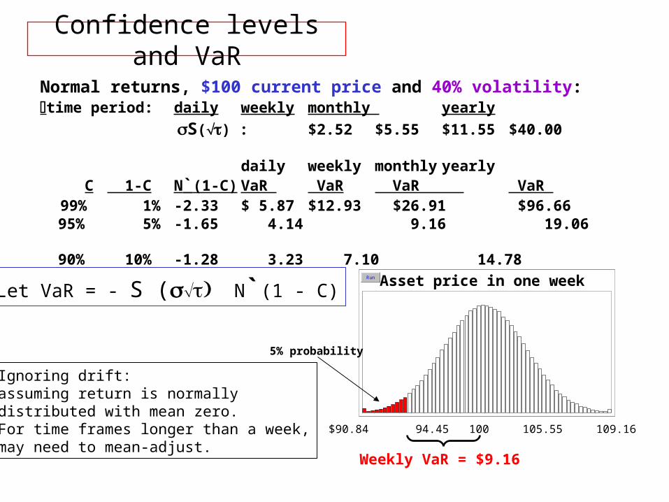
Confidence levels and VaR
Normal returns, $100 current price and 40% volatility:time period: daily weekly monthly yearly
S() : $2.52 $5.55 $11.55 $40.00
daily weekly monthly yearly C 1-C N`(1-C) VaR VaR VaR VaR 99% 1% -2.33 $ 5.87 $12.93 $26.91 $96.66 95% 5% -1.65 4.14 9.16 19.06 90% 10% -1.28 3.23 7.10 14.78
Let VaR = - S ( N`(1 - C)Run Asset price in one week
$90.84 94.45 100 105.55 109.16
Ignoring drift: assuming return is normallydistributed with mean zero.For time frames longer than a week,may need to mean-adjust.
5% probability
Weekly VaR = $9.16
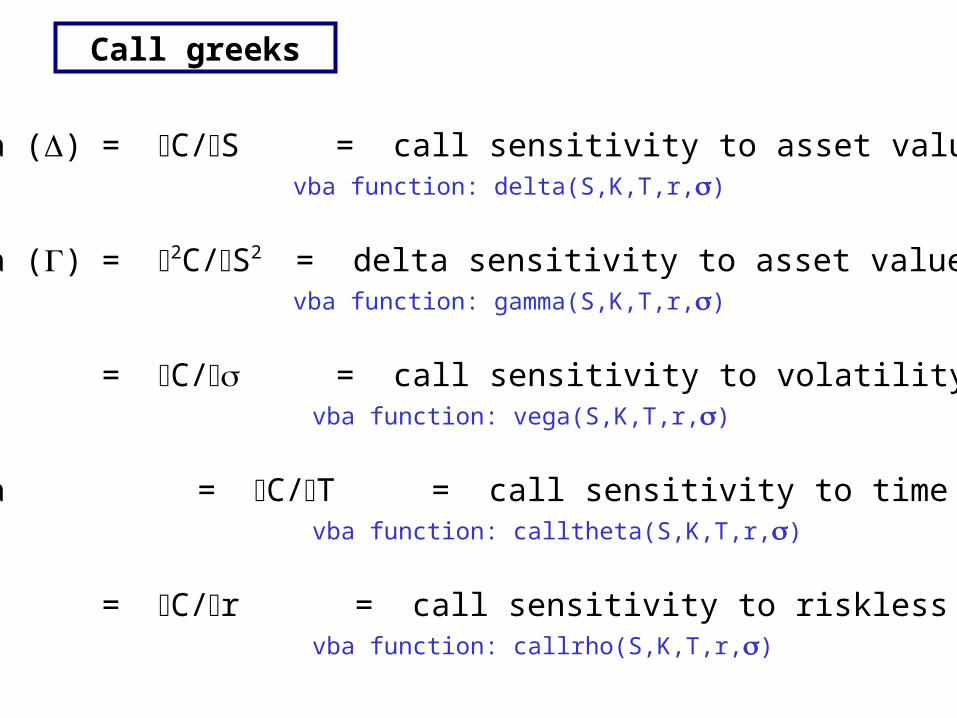
delta () = C/S = call sensitivity to asset valuevba function: delta(S,K,T,r,)
gamma () = 2C/S2 = delta sensitivity to asset value
vba function: gamma(S,K,T,r,)
vega = C/ = call sensitivity to volatility vba function: vega(S,K,T,r,)
theta = C/T = call sensitivity to time vba function: calltheta(S,K,T,r,)
rho = C/r = call sensitivity to riskless rate vba function: callrho(S,K,T,r,)
Call greeks
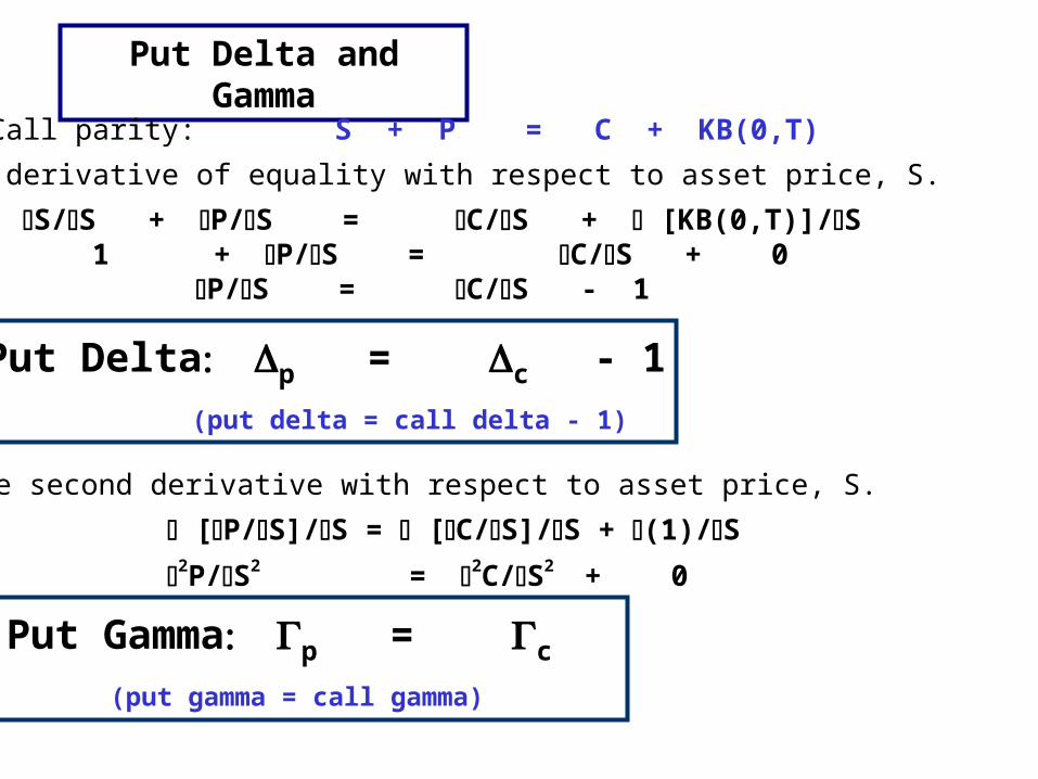
Put Delta and Gamma
Put-Call parity: S + P = C + KB(0,T)
take derivative of equality with respect to asset price, S.
S/S + P/S = C/S + [KB(0,T)]/S 1 + P/S = C/S + 0 P/S = C/S - 1
Put Deltap = c - 1
(put delta = call delta - 1)
Take second derivative with respect to asset price, S.
[P/S]/S = [C/S]/S + (1)/S
2P/S2 = 2C/S2 + 0
Put Gammap = c
(put gamma = call gamma)
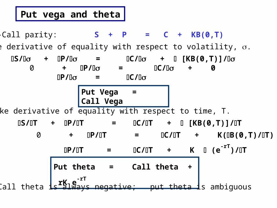
Put vega and theta
Put-Call parity: S + P = C + KB(0,T)
take derivative of equality with respect to volatility, .
S/ + P/ = C/ + [KB(0,T)]/ 0 + P/ = C/ + 0 P/ = C/
Put Vega = Call Vega
take derivative of equality with respect to time, T.
S/T + P/T = C/T + [KB(0,T)]/T
0 + P/T = C/T + K(B(0,T)/T)
P/T = C/T + K (e-rT)/T
Put theta = Call theta + rK e-rT
Call theta is always negative; put theta is ambiguous
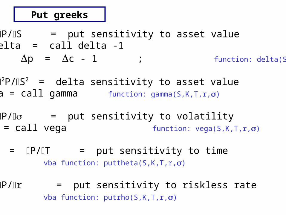
Put greeks
delta () = P/S = put sensitivity to asset value put delta = call delta -1 p = c - 1 ; function: delta(S,K,T,r,) - 1
gamma () = 2P/S2 = delta sensitivity to asset valueput gamma = call gamma function: gamma(S,K,T,r,)
vega = P/ = put sensitivity to volatilityput vega = call vega function: vega(S,K,T,r,)
theta = P/T = put sensitivity to time vba function: puttheta(S,K,T,r,)
rho = P/r = put sensitivity to riskless rate vba function: putrho(S,K,T,r,)
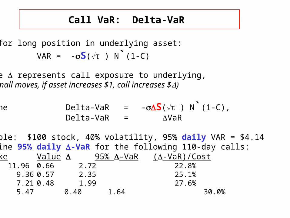
Call VaR: Delta-VaR
VaR for long position in underlying asset:
VAR = -S( ) N`(1-C)
Since represents call exposure to underlying,(for small moves, if asset increases $1, call increases $)
define Delta-VaR = -S( ) N`(1-C),e.g. Delta-VaR = VaR
example: $100 stock, 40% volatility, 95% daily VAR = $4.14Examine 95% daily -VaR for the following 110-day calls:Strike Value 95% -VaR (-VaR)/Cost 95 11.96 0.66 2.72 22.8%100 9.36 0.57 2.35 25.1%105 7.21 0.48 1.99 27.6%110 5.47 0.40 1.64 30.0%
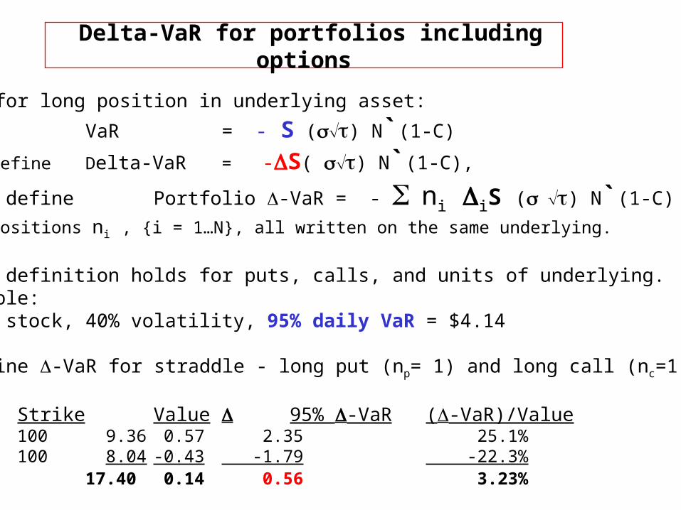
Delta-VaR for portfolios including options
VaR for long position in underlying asset:
VaR = - S () N`(1-C)
and define Delta-VaR = -S( ) N`(1-C),
then define Portfolio -VaR = - ni iS () N`(1-C)
for positions ni , {i = 1…N}, all written on the same underlying.
This definition holds for puts, calls, and units of underlying.example:$100 stock, 40% volatility, 95% daily VaR = $4.14
Examine -VaR for straddle - long put (np= 1) and long call (nc=1):
Strike Value 95% -VaR (-VaR)/Valuecall 100 9.36 0.57 2.35 25.1%put 100 8.04 -0.43 -1.79 -22.3%total 17.40 0.14 0.56 3.23%
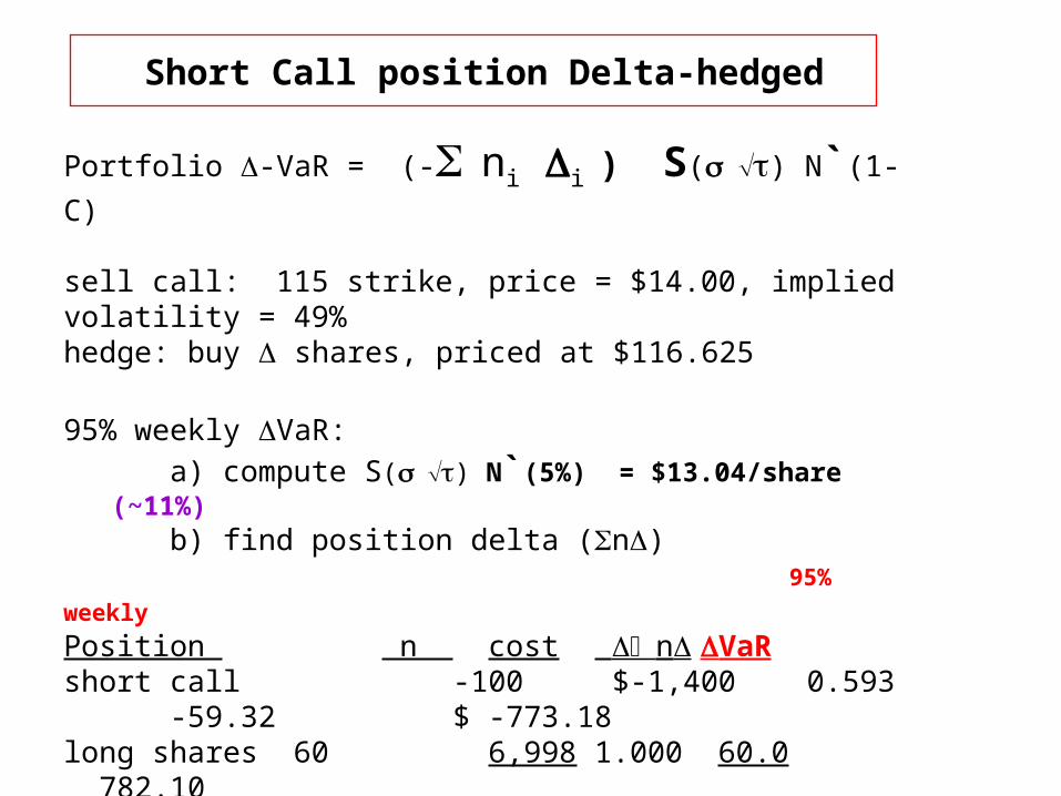
Short Call position Delta-hedged
Portfolio -VaR = (- ni i ) S() N`(1-C)
sell call: 115 strike, price = $14.00, implied volatility = 49%hedge: buy shares, priced at $116.625
95% weekly VaR:
a) compute S() N`(5%) = $13.04/share (~11%) b) find position delta (n)
95% weekly
Position n cost n VaRshort call -100 $-1,400 0.593 -59.32 $ -773.18long shares 60 6,998 1.000 60.0 782.10total $ 5,609 0.68 $ 8.92
95% weekly VaR/cost = $9/5609 = 0.16%
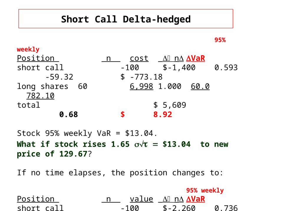
Short Call Delta-hedged
95% weekly
Position n cost n VaRshort call -100 $-1,400 0.593 -59.32 $ -773.18long shares 60 6,998 1.000 60.0 782.10total $ 5,609 0.68 $ 8.92
Stock 95% weekly VaR = $13.04.
What if stock rises 1.65 $13.04 to new price of 129.67?
If no time elapses, the position changes to: 95% weekly
Position n value n VaRshort call -100 $-2,260 0.736 -73.60 $ -1067.00long shares 60 7,780 1.000 60.0 870.00total $ 5,520 -13.60 $ -197.00
loss in value = $89.00 !
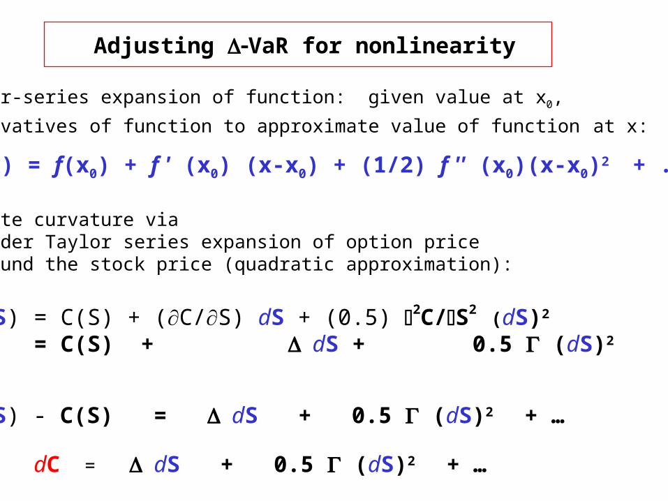
Adjusting VaR for nonlinearity
Use Taylor-series expansion of function: given value at x0,
use derivatives of function to approximate value of function at x:
f(x) = f(x0) + f ' (x0) (x-x0) + (1/2) f '' (x0)(x-x0)2 + ...
Incorporate curvature viaSecond-order Taylor series expansion of option price
around the stock price (quadratic approximation):
C(S + dS) = C(S) + (C/S) dS + (0.5) 2C/S2 (dS)2
= C(S) + dS + 0.5 (dS)2
so that
C(S + dS) - C(S) = dS + 0.5 (dS)2 + …or
dC = dS + 0.5 (dS)2 + …
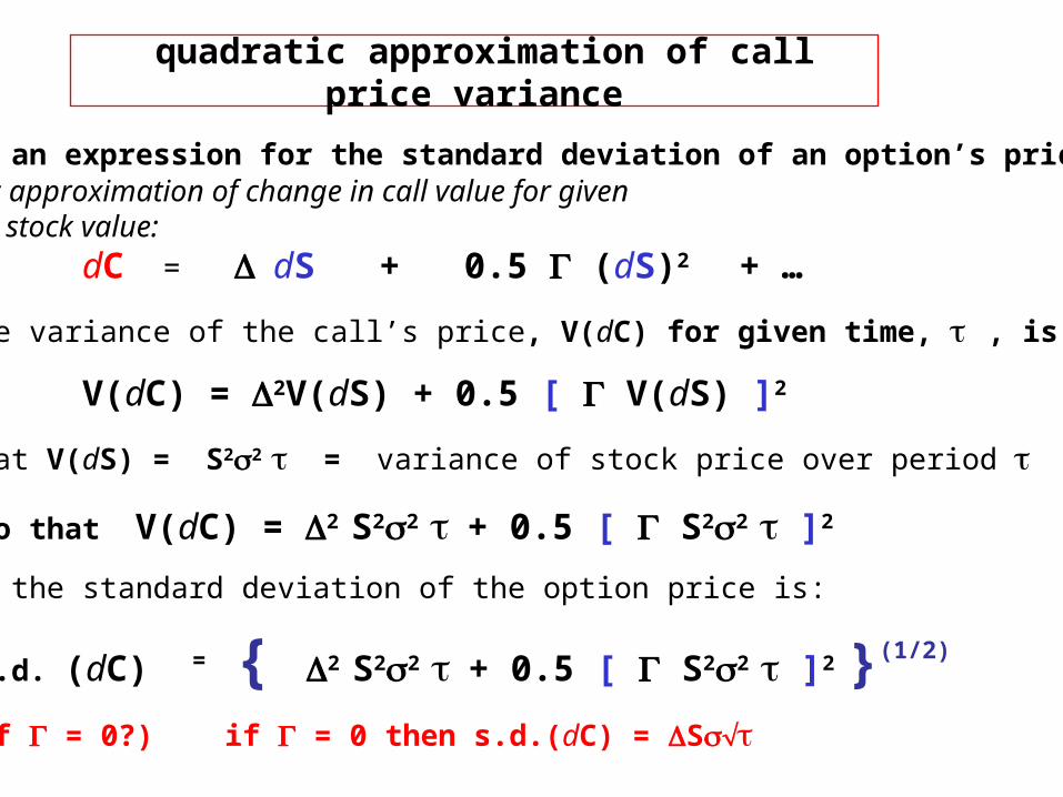
quadratic approximation of call price variance
we want an expression for the standard deviation of an option’s price Quadratic approximation of change in call value for givenchange in stock value:
dC = dS + 0.5 (dS)2 + …
then the variance of the call’s price, V(dC) for given time, , is:
V(dC) = 2V(dS) + 0.5 [ V(dS) ]2
note that V(dS) = S22 = variance of stock price over period
so that V(dC) = 2 S22 + 0.5 [ S22 ]2
thus the standard deviation of the option price is:
s.d. (dC) = { 2 S22 + 0.5 [ S22 ]2 }(1/2)
(what if = 0?) if = 0 then s.d.(dC) = S
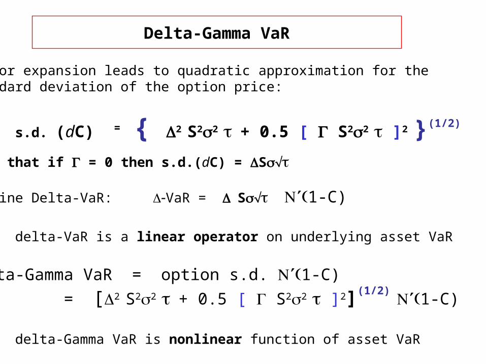
Delta-Gamma VaR
Taylor expansion leads to quadratic approximation for the standard deviation of the option price:
s.d. (dC) = { 2 S22 + 0.5 [ S22 ]2 }(1/2)
Note that if = 0 then s.d.(dC) = S
Examine Delta-VaR: VaR = S1-C)
delta-VaR is a linear operator on underlying asset VaR
Delta-Gamma VaR = option s.d. 1-C)
= [2 S22 + 0.5 [ S22 ]2](1/2) 1-C)
delta-Gamma VaR is nonlinear function of asset VaR
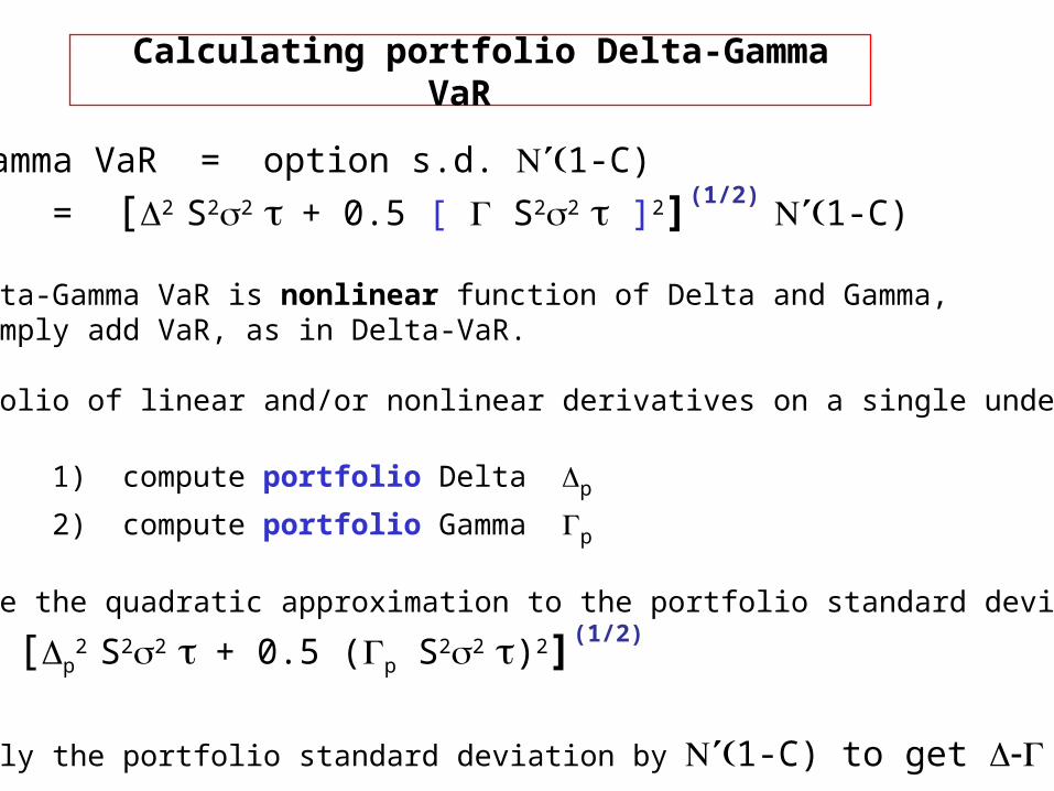
Calculating portfolio Delta-Gamma VaR
Delta-Gamma VaR = option s.d. 1-C)
= [2 S22 + 0.5 [ S22 ]2](1/2) 1-C)
Since Delta-Gamma VaR is nonlinear function of Delta and Gamma,cannot simply add VaR, as in Delta-VaR.
For portfolio of linear and/or nonlinear derivatives on a single underlying:
Solution: 1) compute portfolio Delta p
2) compute portfolio Gamma p
3) compute the quadratic approximation to the portfolio standard deviation
[p2 S22 + 0.5 (p S22 )2](1/2)
4) multiply the portfolio standard deviation by 1-C) to get VaR
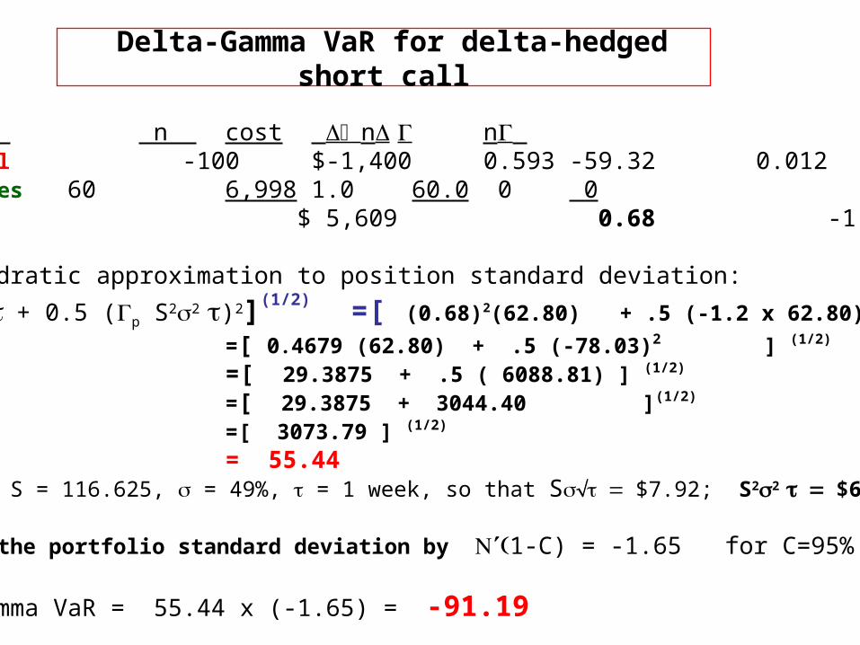
Delta-Gamma VaR for delta-hedged short call
Position n cost n n short call -100 $-1,400 0.593 -59.32 0.012 -1.2long shares 60 6,998 1.0 60.0 0 0total $ 5,609 0.68 -1.2
Find quadratic approximation to position standard deviation:
[p2 S22 + 0.5 (p S22 )2](1/2) =[
(0.68)2(62.80) + .5 (-1.2 x 62.80)2 ] (1/2)
=[ 0.4679 (62.80) + .5 (-78.03)2 ] (1/2) =[ 29.3875 + .5 ( 6088.81) ] (1/2)
=[ 29.3875 + 3044.40 ](1/2) =[ 3073.79 ] (1/2)
= 55.44 (using S = 116.625, = 49%, = 1 week, so that S$7.92; S22 $62.80)
Multiply the portfolio standard deviation by 1-C) = -1.65 for C=95%
Delta-Gamma VaR = 55.44 x (-1.65) = -91.19
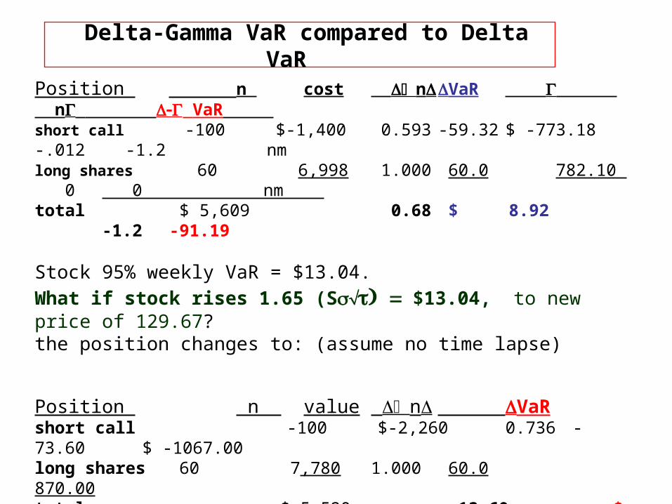
Delta-Gamma VaR compared to Delta VaR
Position n cost n VaR n VaR
short call -100 $-1,400 0.593 -59.32 $ -773.18 -.012 -1.2 nmlong shares 60 6,998 1.000 60.0 782.10 0 0 nm total $ 5,609 0.68 $ 8.92 -1.2 -91.19
Stock 95% weekly VaR = $13.04.
What if stock rises 1.65 (S$13.04, to new price of 129.67?the position changes to: (assume no time lapse)
Position n value n VaRshort call -100 $-2,260 0.736 -73.60 $ -1067.00long shares 60 7,780 1.000 60.0 870.00total $ 5,520 -13.60 $ -197.00
loss in value = $89.00 - a bit less than VaR = 91.19
If position is unchanged, moves to -0.9 and the new VaR = $214.90
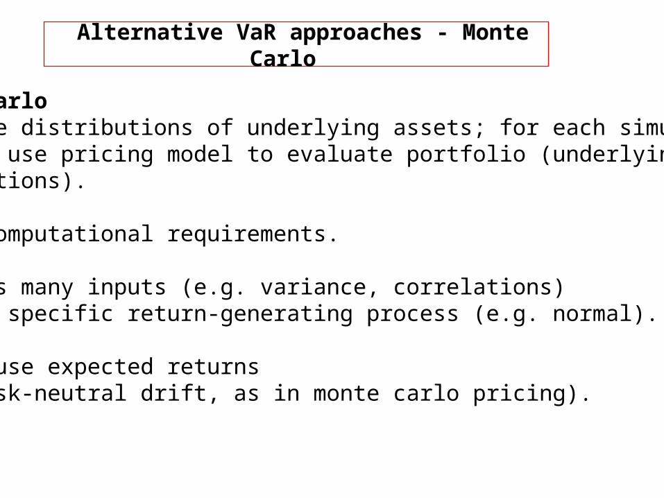
Alternative VaR approaches - Monte Carlo
Monte Carlosimulate distributions of underlying assets; for each simulatedoutcome use pricing model to evaluate portfolio (underlying and options).
Heavy computational requirements.
Requires many inputs (e.g. variance, correlations)Assumes specific return-generating process (e.g. normal).
Should use expected returns(not risk-neutral drift, as in monte carlo pricing).
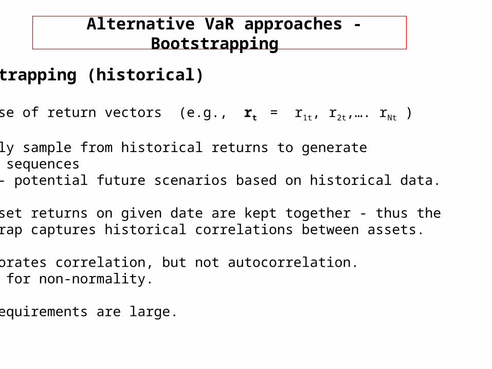
Alternative VaR approaches - Bootstrapping
Bootstrapping (historical)
database of return vectors (e.g., rt = r1t, r2t,…. rNt )
randomly sample from historical returns to generate return sequences
- potential future scenarios based on historical data.
All asset returns on given date are kept together - thus the bootstrap captures historical correlations between assets.
Incorporates correlation, but not autocorrelation.Allows for non-normality.
Data requirements are large.
references
Chance, Don, 1998. An Introduction to Derivatives. The Dryden Press.
Jorion, Phillipe, 1997. Value at Risk: The New Benchmark for controlling market risk. Irwin Professional Publishing.
Stulz, Rene, 1999. Derivatives, Financial Engineering, and Risk Management. South-Western College Publishing (in press).
Wilmott, Paul, 1998. Derivatives - The Theory and Practice of Financial Engineering. John Wiley & Sons. (www.wilmott.com)


![[XLS]options.live 4.12 - Texas Christian Universitysbufaculty.tcu.edu/mann/Fin 70520 Spring 2002... · Web viewOptions.live 6.01 provides T-bill discounts as of 11.12.2001 This version:](https://img.pdfslide.net/doc/110x75/5aef1da77f8b9a572b8da255/xls-412-texas-christian-universitysbufacultytcuedumannfin-70520-spring.jpg)