Embed Size (px)
Citation preview

It is the policy of the University of Nebraska–Lincoln not to discriminate based upon age,race, ethnicity, color, national origin, gender, sex, pregnancy, disability, sexual orientation,
genetic information, veteran’s status, marital status, religion or political affiliation.
© 2012, The Board of Regents of the University of Nebraska on behalf of theUniversity of Nebraska–Lincoln Extension. All rights reserved.
Heifer Breeding Maturity and Its Effects on Profitability: Nebraska Sandhills Beef Cattle
Matthew C. StocktonAgricultural EconomistWest Central Research and Extension
CenterUniversity NebraskaNorth Platte, NE 69101
Roger K. WilsonEconomics AnalystUniversity NebraskaLincoln, NE 68583
Rick FunstonReproductive PhysiologistWest Central Research and Extension
CenterUniversity NebraskaNorth Platte, NE 69101
Dillon FeuzAgricultural EconomistUtah State UniversityLogan, UT 84322
Aaron StalkerRuminant NutritionistWest Central Research and Extension
CenterUniversity NebraskaNorth Platte, NE 69101
RB350

Table of Contents
Abstract .......................................................................................................................................................................................... 5
Introduction .................................................................................................................................................................................. 5
Maturity Index (MI)............................................................................................................................................................ 5
The Inclusion of Economics ............................................................................................................................................... 6
Individual Animal vs. Group Data ..................................................................................................................................... 7
Literature Review (Background) .................................................................................................................................................. 8
Data ................................................................................................................................................................................................10
Procedures .....................................................................................................................................................................................11
Guided Regression Choice Methodology (GRCM) ...........................................................................................................11
Defining Pre-breeding Size — the Maturity Index ............................................................................................................11
The Modified Profit Function (MPF) ................................................................................................................................13
Revenue ................................................................................................................................................................................13
Cost ......................................................................................................................................................................................14
Pregnancy and Dystocia Rates ............................................................................................................................................14
Revenue Equation Specifics ................................................................................................................................................20
The Implementation of MPF ..............................................................................................................................................28
The MPF Array ....................................................................................................................................................................29
Results ............................................................................................................................................................................................33
Maturity Index .....................................................................................................................................................................33
The Optimal MI ..................................................................................................................................................................34
Conclusions ...................................................................................................................................................................................38
References ......................................................................................................................................................................................41
Appendix 1. Normalized Success Index of Predicting Pregnancy Using the Maturity Index, Percent of Herd Average Weight, and Percent of Dam Mature Weight .................................................................................................................42
Appendix 2. Predicted Rates/Probabilities of Dystocia Predicted by Linear, Quadratic, and Cubic Forms of the Maturity Index ........................................................................................................................................................43
Appendix 3. Normalized Success Index of Predicting Dystocia Using Linear, Quadratic, and Cubic Forms of the Maturity Index ........................................................................................................................................................44
Appendix 4. Normalized Success Rate for Predicting Pregnancy Using Actual and Predicted Dystocia .................................45
Appendix 5. List of Models ...........................................................................................................................................................46
Appendix 6. 2003, 2004, and 2005 Modified Profit Function Results ........................................................................................50

Table of Figures
Figure 1. Predicted dystocia rates as forecast by maturity index measures using three different probit specifications for I ..17
Figure 2. Estimated second pregnancy rates as a function of the maturity index .....................................................................18
Figure 3. Estimated second pregnancy rates as a function of dystocia rate ...............................................................................19
Figure 4. Maturity index as a predictor of age of heifer’s first calf at weaning ..........................................................................23
Figure 5. Sample array taken directly from a Microsoft’s Excel® workbook ..............................................................................30
Figure 6. The impact of age at weaning on weight at weaning ...................................................................................................31
Figure 7. Predicted pre-breeding weights by ration and age of dam ..........................................................................................32
Figure 8. Comparison of maturity index to percent of herd average weight .............................................................................33
Figure 9. Graph of the effects of the maturity index on the modified profit function score, total applied revenues, and total applied costs mega-analysis results ..............................................................................................................................35
Figure 10. 2003 modified profit function scores for various maturity indices for Ration 1 .....................................................36
Figure 11. 2003 modified profit function scores for various maturity indices for Ration 2 .....................................................36
Figure 12. 2003 modified profit function scores for various maturity indices for Ration 3 .....................................................37
Figure 13. 2003 modified profit function scores for various maturity indices for Ration 4 .....................................................37
Figure 14. 2003 modified profit function scores for various maturity indices for all rations ...................................................38

Table of Tables
Table 1. Comparison of independent variables in the rate of first pregnancy probit results ....................................................15
Table 2. Normalized success index (NSI) for dystocia using three different forms of MI ........................................................16
Table 3. Comparison of the methods used for estimating maturity’s effect on second pregnancy ..........................................19
Table 4. Annual adjustments from 2006 for bred cow prices......................................................................................................26
Table 5. Feed intake and ration composition on an “as fed” basis by treatment group ............................................................27
Table 6. Prices of feedstuffs used in formulating the protein supplement .................................................................................27

© The Board of Regents of the University of Nebraska. All rights reserved. 5
Heifer Breeding Maturity and Its Effects on Profitability:
Nebraska Sandhills Beef Cattle
Abstract
The question of determining the size at which to breed beef replacement heifers is not a new one. This research differs from most in the literature in three major ways. First, analysis of biological relationships is done on the basis of individual animals rather than experimental groups. Second, outcomes from biological analysis are used to simulate results that are analyzed. Finally, analyzed results are in terms of profitability rather than biological measures. The basis for identifying biological relationships used in the simulation are a series of integrated models (regression equations) derived by using the AKAIKE loss criterion to optimally select those relationships expressed as equations from individual animal data. The final simulation uses the relationships indentified in the biological subsystems and translates them through the appropriate economic condi-tions (cost and revenue) to determine a cow profitability score or Modified Profit Function (MPF). Results show optimal profitability depends on relationships among a number of factors rather than any one or two individual factors. Because results depend on relationships among factors, an index is presented as a tool for replacement heifer selection.
Introduction
While the question of determining the optimal size at which to breed beef replacement heifers has been studied in some detail, the complexity and an ever changing industry invite updating and improvement in the methodologies and study of this topic. As beef production becomes increasingly more competitive, reproductive rates, growth rates, and calf mortality rates are ever under pressure to improve. One of the key elements in maintaining a profitable operation is to use all resources economically.
A substantial cost to producers is the development or purchase of replacement females. Each year beef cattle producers in Nebraska retain as many as 21% of their calves as replacements, with the average being 17% (Clark et al. 2002). With so much of the producer’s success riding on the proper care, development, and cost of supplying replacement heifers, it is no wonder that the literature is filled with research devoted to deter-
mining the ideal maturity at which replacement females should be developed. The relationships among nutrition, growth, and sexual development are well documented. However, prior studies do not use profit as the factor that is optimized when determining time or size to breed. This research differs from most in the literature in that it examines the issue from an integrated systems approach including economics, rather than strictly a biological one. The methodology for this analysis derives biological relationships and interrelationships and associates them appropriately with the economic system.
The physical models are derived using regression techniques to analyze differences among individual animals as opposed to the commonly accepted practice of using analysis of variance statistical methods to compare treatment groups. This work is a genuine collaborative effort, where the animal scientists and economist have worked closely in the construction and development of the complete project. The animal data for this project are from research conducted by repro-ductive physiologists at University of Nebraska–Lincoln’s West Central Research and Extension Center (Funston and Deutscher 2004 and Martin et al. 2008). The appli-cation of economic and the construction of the physical portions of that model were done by the economist with input from the biological scientist.
Maturity Index (MI)
The challenges associated with defining a heifer’s size at pre-breeding immediately became apparent when analyzing individual animal data. Pre-breeding maturity is traditionally measured as a percent of the animal’s mature weight, where the heifer’s weight at the time of breeding is a percent of her mature weight (PMBW). Beef cattle are expected to reach their mature weight between 4 and 5 years of age, which generally occurs 30 months after the first breeding cycle. This fact presents several challenges. First, it is impossible to know what that mature weight is at the time of first breeding or earlier when heifers are selected as replacement animals since mature weight is not known until years after these decisions are made. For this reason, scientists and producers generally use an average mature weight to approximate the pre-breeding weight percentage. The

6 © The Board of Regents of the University of Nebraska. All rights reserved.
percent of herd average weight (PHAW) was used as a proxy by Funston and Deutscher (2004) and Martin et al. (2008) in the original heifer development study.
While using PHAW as a proxy for mature weight is widely accepted, it is problematic and serves to add noise in the analysis. The noise is increased as variation in individual animal’s weight increases within the group of animals being analyzed. The weights of mature cows in the University of Nebraska’s Gudmundsen Sandhills Laboratory (GSL) herd vary from 800 to 1,400 pounds. In this case, the average mature weight for cows is 1,151 pounds. As an example, a heifer from this herd weighing 750 pounds at pre-breeding would have a PHAW close to 65%. However, if the actual mature weight of that 750 pound heifer is 950 pounds; her true PMBW would be 79%. In the opposite case where her mature weight is 1,400 pounds, the same 750 pre-breeding weight results in a 53% PMBW. Using 65% in an analysis when 53% or 79% is the true PMBW introduces bias in the selection and performance process. This variation (noise) creates imprecision in the analysis, making the results unreliable and inapplicable.
Developing a new methodology of determining a heifer’s reproductive maturity is a major component and contribution of this research. In effect, the need to measure maturity of heifers is a forecasting problem. Economists have developed well-established techniques to build forecasting models. Through the use of these econometric techniques, a model was developed that forecasts the reproductive maturity of heifers at the time of the first breeding cycle; it is referred to here as the maturity index or MI. It turns out that forecasting repro-ductive maturity is not overly complex. Factors used in the index include the heifer’s age, nutrition, birth weight, dam’s age and dam’s mature weight. As with all good forecasting models, the factors used are easily observed prior to the event. This gives the model the advantage of being based on observable information and known relationships, rather than the traditional model which is based on an expected average size.
The Inclusion of Economics
The solutions identified in this work are based on a modified profit function (MPF) which translates physical characteristics of individual animals into a profit score. Modern animal science research commonly includes some economic components, but generally does not finely focus their results through the lens of a system and a profit function. This methodology focuses on the “bottom-line.” Basing the analysis on changes to profit-ability provides results that are directly applicable and easily understood.
A simple explanation of the difference between a physical optimum versus an economic one will illus-trate why economics is the focus for this work. Natural systems exhibit a diminishing marginal effect. As units of inputs are increased, the corresponding gains in production diminish at some point. This is commonly referred to as the law of diminishing returns (Epp and Malone Jr., 1981, p 35). A quadratic production function to represent the effect of nitrogen application to corn yield will be used to demonstrate this point. Increasing the amount nitrogen fertilizer applied to corn from 100 to 125 pounds per acre increases yield by 20.3 bushels per acre. The application of the next 25 pounds of nitrogen increases yields per acre by 14.2 bushels. And the application of the next 25 pounds increases per acre yields by 8.0 bushels. Each succeeding addition of fertilizer has a diminishing effect on yield. In this example, maximum production occurs at 196 pounds of nitrogen. The last pound of nitrogen produced .0083 bushels of corn per acre. If fertilizer costs $0.60 per pound, and corn is valued at $5.00 per bushel, profit for this last unit of fertilizer would be a negative $.56. Knowing this, a producer would be economically rational to apply fertilizer only where the return from its application were at least as much as its cost. This is known as profit maximizing behavior. In this example, the producer would limit the use of fertilizer to between 183 and 184 pounds of nitrogen applied per acre. This rate is lower than the yield maximizing amount of 196 pounds of nitrogen applied per acre.
Profit is a useful and comprehensive measure that accounts for contributions of those factors that change both costs and revenues. While profit maximizing behavior may not be the only motivator for business owners in making decisions, it is a measurable and logical indicator of behavior. That is why this method-ology is a viable basis for determining the optimal replacement heifer size at the time of first breeding.
The original vision for this work was to build a simple profit function using relationships among heifer size at breeding and pregnancy and dystocia rates, and optimize it using calculus; similar to the work done by Feuz (1991). However, in doing the analysis it was deter-mined that reproductive maturity involved multiple facets, rendering this simple approach inadequate and unsatisfactory. It became apparent that the maturity and productivity of heifers is driven by many different condi-tions.
The MI was developed by which these multiple conditions are combined into a single number. This index utilizes multiple variables, which creates the inherent problem of identification since each MI can be associated with many different combinations of

© The Board of Regents of the University of Nebraska. All rights reserved. 7
variables. For example, two heifers having the same index could have different weights, ages, birth weights, and/or dam sizes. This fact renders a calculus-derived answer impotent. This, along with the fact that the usefulness of a single-point solution is limited, leads to an alternative method of analysis.
In addition to the identification problem, the modified profit function (MPF) is more complex than anticipated due to the nature of some of the relation-ships within the system, and proper differentiation, if not impossible, requires many restrictions which decrease its value. With these observations in mind, the most promising alternative method is a numerical method-ology.
The numerical approach is a brute force method-ology that calculates profit using all of the appropriate combinations of input variables, and allows for a complete analysis of the results to account for a variable’s impact on profitability. The values of the variables used in the numerical method are constrained to the finite range of feasibility. For example, it is not feasible for a cow weighing 800 pounds at maturity to give birth to a 120-pound calf. Regression equations using ordinary least squares were applied to the observed data to derive the appropriate feasibility range for all variables in the analysis.
Profit is defined as the difference between total revenue and total cost. However, not all revenues and costs are related to heifer size at pre-breeding. For instance, cost for breeding does not change as the size of the replacement heifer varies. This is true for some other costs and revenues as well.
To simplify the profit function as much as possible, it is modified to include only those revenues and costs that change as heifer size changes. Since some costs and revenues are not included in the MPF, the function does not calculate actual profitability but instead produces a dollar profit score which is easily used to compare results and rank individual heifers. This methodology, while not providing an estimate of absolute profitability, does provide a basis for comparing the relative profitability when designated inputs are varied.
Five sources of revenue are included in the MPF: 1) The sale of replacement heifers that fail to become pregnant with their first calf, 2) The sale of heifers that fail to have a first calf or lose their calf by the time they are put on summer pasture, 3) The sale of calves produced by replacement heifers, 4) The sale of cows that are found not to be pregnant at the time their first calf is weaned, 5) The value of those cows that were diagnosed as being pregnant with their second calf at the time
their first calf is weaned. Cow productivity beyond the time of the first calf ’s weaning is not included here. This constraint eliminates the consideration of any effects a heifer’s size at pre-breeding has on cow longevity or continued productivity, and is beyond the scope of this work.
Three cost centers are included in the MPF: 1) The cost of acquiring a weaned calf as a replacement for a female culled from the herd — opportunity cost, 2) The cost of feeding these replacement females to pre-breeding weight/size/maturity, 3) The cost associated with dystocia — calving difficulty. As indicated, these variables each have a direct association with size, devel-opment, and/or productivity of the replacement heifer.
Individual Animal vs. Group Data
Typically, animal science research uses random-ization to place animals into treatment groups. Group averages for specified traits are compared statistically, usually applying an analysis of variance, or ANOVA, methodology. The use of randomization to assign animals to groups is a procedure used to eliminate the effects of factors not being studied. The statistical comparison of traits from randomized groups of animals to determine the effects of a treatment is a powerful tool and solid science. However, as with all methodologies, there are implications associated with its use.
While this methodology enables scientists to control the experiment and test for effects of single variables, it eliminates the effects of some factors that might have significant bearing on the question being asked. In the experiments by Funston and Deutscher (2004) and Martin et al. (2008), differences in heifer size because of feeding programs were analyzed, but differences in size because of genetic potential or other factors were eliminated in the randomization process. The effect that genetic potential has on heifer size at the first breeding period, or how this potential responds to nutritional requirements for reproductive success, were not included in their experimental design. Other factors hidden by randomizing animals into groups are discussed later in this work.
In contrast, economic analysis generally uses individual observations of secondary data; data that is not obtained by controlled experiments. For this reason, economists have designed tools and methods, known as econometrics, to determine the effects that multiple independent factors might have on an outcome. Econo-metrics has two primary methodologies; a structural and an atheoretical approach. Each method plays a role in this work.

8 © The Board of Regents of the University of Nebraska. All rights reserved.
The structural approach is one where external observation, logical thinking, and accepted theory guide the construction of appropriate relationships among the variables selected to be included in the model. The atheoretical approach is a data driven approach where it is assumed the relational information is inherit in the data itself. This method relies upon a loss function to determine which statistically significant relationships are to be included in the model. The loss function is designed to weight the benefits of the number of explan-atory variables versus the explanatory value of each variable. The best model is identified as having the lowest loss function score. This method follows closely with the Occam Razor principle - the simplest explanation is usually the best.
The use of econometric techniques makes it possible to include factors that exploit individual animal variation, and expand the findings of the original studies. In a regression equation, each animal becomes a unique source of information while the treatment groups used in the original studies are accounted for using dummy, control variables, or indicator variables. This approach expands the usefulness of the data and its potential to derive relationships pertinent to the economic outcome and profit function. Variables considered for inclusion in the analysis are heifer age at first breeding cycle, birth weight, mature size of subject’s dam, and the dam’s age at the time of the heifer’s birth.
Using this methodology also provides an additional advantage when studying the issue of individual heifer retention. Producers generally select animals based on individual merit, not as a group. This method relates to the belief that the individual replacement heifer’s charac-teristics relate to, or are at least partially control, the individual animal’s future performance. This approach is consistent with the development and use of the models/equations in this work. These models are designed to relate directly to observable animal characteristics which relate them in a system linked to performance and profitability. This process is consistent with the process producers are following when they select a heifer based on her estimated individual performance.
The use of an econometric type methodology is not novel and has been used in various forms in studies within the animal science discipline. This fact is illus-trated in works such as Hadley et al. (2006), Eler et al. (2002), Doyle et al. (2000), Evens , (1999), Varona et al. (1999), and Greer et al. (1983). These studies are discussed in greater detail in the Literature Review section.
One of the challenges in doing analyses on individual animals is appropriately relating maturity to
first pregnancy, dystocia, and second pregnancy; three of the primary variables contained within the revenue and cost portions of the MPF. Both pregnancies and dystocia are qualitative in that the animal is in one of two states. In the case of pregnancy, the heifer is either pregnant or not pregnant. With calving difficulty, or dystocia, the heifer is either observed as delivering her calf with or without assistance. Economists have historically used limited dependant variable regression methodologies to properly address this challenge and to derive appropriate estimates and interpretation of the estimated factors or drivers. Limited dependant variable modeling, as the name suggests, limits the value of the left-hand side, or dependant variable in this case, to being less than one and greater than zero.
Limited dependant variable models take on different forms depending on the type of probability function on which they are based. We adopt the probit regression model for both pregnancy and dystocia. The probit methodology is a limited dependant variable model that relies on the normal distribution function for interpre-tation (Griffiths, Hill, and Judge 1993, page 740-760). While this methodology may be unfamiliar to some, it has been used in studies of genetic heritability (such as Doyle et al. 2000, Eler et al. 2002, Evans et al. 1999, and Varona et al. 1999) and dairy cattle culling (Hadley ,et al. 2006).
The interpretation of the probit regression’s coefficient estimates of independent (right-hand side) variables predict the effect they have on the probability of occurrence of the dependant (left-hand-side) variable. Hadley (2006) used economic factors, farm and cow characteristics as independent or predictor variables (right-hand-side). The dependent or predicted trait (left-hand-side) was the probability that an individual cow was culled. In this case, the estimated coefficients indicate that cow age is positively related to the probability of the cow being culled. For example he showed that the older the cow, the more likely she would be culled.
Literature Review (Background)
Animal science and agricultural economics literature both contain a number of studies evaluating strategies for managing replacement beef heifers prior to breeding. Patterson’s et al. (1992) review of the literature summa-rizes the findings of some of these. Heifer weight is used as a proxy for maturity and is the focal point in many of the studies reviewed. Generally, heifers fed at a higher plain of nutrition gain more weight and tend to have higher rates of pregnancy. However, the heavier the heifer the greater their cost. Determining when increased costs exceed the gains resulting from higher conception rates is

© The Board of Regents of the University of Nebraska. All rights reserved. 9
critical (Greer et al. 1983). Greer (1983) concludes that considering differences among cattle types and breeds, the absolute weight of the animal lacks value in deter-mining breeding readiness, and thus, suggest that general weight recommendations are difficult to specify. Greer further theorizes that an “index of maturity” exists and makes an attempt to estimate that index by using weight at first estrus divided by yearling fall weight. His attempt was unsuccessful and resulted in an index that was not statistically viable.
Patterson et al. (1991) uses a target weight for beef heifers at the first breeding cycle as a measure of breeding readiness. To account for differences between cattle types and breeds, he defines target weight as PMBW (which is described above) but uses the PHAW method. Current physical stature as a percent of actual mature size is a quantifiable relative measure and can be widely applied. However, because mature body weight is not available until well after the age at which heifers are selected for retention, frame measurements were used to estimate heifers’ mature sizes. Unfortunately, they chose to average the measurements by breed group rather than individual frame scores. These averages, along with breed averages, were used to estimate the mature weight of their groups. They reported (but did not document their source) that 65 PMBW was the recommended norm but 55 PMBW reflected the industry average. Patterson et al. (1992) concludes, “Until a better rule of thumb is established, the target weight principle of developing heifers to an optimum pre-breeding weight seems to be the most feasible method of ensuring that a relatively high percentage of yearling heifers reach puberty by the breeding season.”
In this same work, Patterson et al. (1991) identified several factors that impact reproductive performance including nutrition and frame size. They conclude that the response to feed restriction tends to decrease reproductive performance more dramatically for large framed heifers, a fact borne out in this work. They also report that the incidence of calving problems increased as nutrition levels decrease and heifers are smaller at calving.
As indicated earlier, researchers at the University of Nebraska West Central Research and Extension Center conducted two consecutive studies that compare different pre-breeding target weights (Funston and Deutscher, 2004; Martin et al. 2008). These researchers hypothesize that heifers developed to the lighter pre-breeding weights may be more economically viable, which supports the observation that the industry standard is a 55 PMBW. Both Nebraska studies randomly divided heifers into two groups that were fed differently. Each group was assigned an average PMBW goal. The
first study compares feeding to a 60 and a 65 PMBW. The second study went even lower, comparing feeding to a 55 and 60 PMBW. Estimated PMBW for these two studies uses the average herd weight of 1,198 and 1,199 pounds, respectively, as a proxy for mature weight and is designated here as PHAW, percent herd average weight. The feed treatments in the Funston and Deutscher study resulted in an estimated percent herd average weight (PHAW) of 58 and 53 for the treatment groups, while the PHAW estimates for the groups in the Martin et al., study were 56 and 51.
Both the Funston and Deutscher, and Martin et al. studies include a financial analysis that includes pregnancy rates and feed cost differences between the treatment groups. The studies found no significant statis-tical differences among pregnancy rates of the groups so it was concluded that those fed less are more economical. Some cost differences among heifers of different sizes, such as the effect that heifer size has on procurement costs, were eliminated from the analysis by the random-ization process. Other cost differences that may have occurred between animals of different sizes, such as those associated with dystocia, were also missing.
The analyses of Funston and Deutscher, and Martin et al. indicate there are no statistical differences in pregnancy rates among treatment groups. This finding only applies to differences in a group’s average PHAW created as an artifact of the treatment factor; nutrition level from weaning to first bull exposure. Variations in maturity due to differences in age at the first breeding cycle, birth weight, and dam’s size and age remain outside of their analysis. These omitted factors are properly considered in this analysis using econometric techniques.
In a paper session at the 1991 Western Agricultural Economics Association annual meetings, Feuz (1991) proposed a procedure to determine optimal beef heifer breeding weight using classical economic methods. Using group average data and ordinary least square regres-sions, he created two models where “target weight” in a quadratic form is included as one of the independent variables. Similar to other research using group average data, Feuz measures target weight as PHAW. He includes first and second calf pregnancy rates and a series of mathematical relationships to incorporate these into a model that estimates profitability. This profit function is then optimized using calculus by setting the first partial derivative of the profit function relative to target weight equal to zero and solving for the optimal target weight. This procedure results in an optimal profit achieved at the target weight of 61 PHAW. This study has never been published in a professional journal due to the limited number of observations contained in the data. This

10 © The Board of Regents of the University of Nebraska. All rights reserved.
work, however, serves as a starting point and framework for basing an analysis on a profit function.
The present study is similar to Feuz’s in that the analysis is based on a profit function and uses econo-metric techniques throughout its development and for analysis. It differs in that it is more complete, identifying many more relationships between the biological perfor-mance of the animals and their respective economic components. It also differs in that the data used for analysis are from individual animals rather than group averages. When using grouped data, pregnancy and dystocia rates are expressed as percent of the group — the number of pregnant females divided by the total number of females in the group, giving a pregnancy rate. The same would be true of dystocia. The number of dystocia incidents is divided by number of heifers in the group that gave birth. In using individual animal data, a binomial result is obtained (an animal is either pregnant or not, dystoctic or not). This fact requires a different methodology in handling the data and doing the analysis. The probit model, as described in the intro-duction, is used to analyze and process these relation-ships.
The probit modeling technique, while not widely found in livestock research literature, has been used. Doyle et al. (2000), Eler et al. (2002), and Evans et al. (1999) used this technique effectively in genetic studies involving heifer pregnancy. These three studies find that the age of the dam and heifer age at pre-breeding are significant factors in the likelihood that a heifer conceives and remains pregnant. Since heritability was the focus of these studies, nutrition and other environmental factors are not included.
Hadley et al. (2006) uses the probit method to study dairy cow culling. In this study of over 7 million Dairy Herd Improvement Association records, various farm and dairy animal characteristics are used to predict the probability that an individual animal will be removed from the herd. The actual process of implementing this type of econometric method is described in the Proce-dures section.
Data
As indicated above, the data for this study were collected by researchers at the University of Nebraska Gudmundson Sandhills Laboratory (GSL) for two consecutive research projects: Funston and Deutscher (2004) and Martin et al. (2008). The earlier study
included 240 heifers that were retained as replacements for the years 1997, 1998, and 1999; the latter study included 260 heifers that were retained for the years 2000, 2001, and 2002. The fact that these two studies are consecutive, continuous, and from the same base cattle herd makes it possible to combine them into a single data set.
The combined data set includes each replacement heifer’s identification number, birth weight and date, weaning weight, pre-breeding weight, dam weight, weight at her first and second pregnancy diagnosis along with her pregnancy status, and the weaning weight of her first calf. If and when an animal left the herd, subse-quent information was recorded as null. Dummy or indicator variables are added to the data set to designate the feed treatment group to which they were assigned. This method was used to allow the regression estimates to recognize the four different levels of nutrition based on ration content and performance group. Indicator or dummy variables are used to designate pregnancy status for both pregnancies and the occurrence of dystocia with the first calf.
Three of the 500 original animals were dropped from the study prior to the first pregnancy check. Of the 497 remaining animals, 448 were diagnosed pregnant with 49 being diagnosed as not pregnant. All nonpregnant heifers were sold. Of the 448 that were diagnosed pregnant, 421 weaned a calf at the end of the calving season. The remaining 27 heifers either did not carry a calf to full term or their calf died prior to weaning. Those animals that failed to produce a calf or lost their calves prior to the end of the first measured calving season were sold, with the exception of one that was found to be pregnant at weaning time. Of the 422, 390 were diagnosed as pregnant with their second calf. Of the 390 diagnosed as pregnant, 302 weaned a third calf and have a recorded mature weight.
Price data used for valuing nonpregnant heifers and the offspring of the pregnant animals comes from the Nebraska livestock auctions as recorded by the United States Department of Agriculture’s (USDA) Agricul-tural Marketing Service (AMS). The recorded prices are available online as a custom report accessible at the Livestock and Grain Market News website (http://marketnews.usda.gov/portal/lg). Utility cow prices were obtained from the Livestock Marketing Information Center database and are the “Monthly Slaughter Cow & Bull Prices” at the Sioux Falls livestock auction market. Bred cow prices were obtained from the Nebraska livestock markets and CattleFax’s Member’s Only website.
© The Board of Regents of the University of Nebraska. All rights reserved. 11
Procedures
Guided Regression Choice Methodology (GRCM)
Animal characteristics and market information that impact profitability are simulated using models derived from regression results. The animal characteristics include the weights of the heifer at birth, weaning, time of first breeding, first pregnancy, spring, and second pregnancy along with the weight of the heifer’s first calf at weaning. Heifer size is a major component of this research; therefore, all price models incorporate weight in the simulations.
Prices for the economic analysis are simulated for heifer price at weaning, first pregnancy diagnosis, late spring cattle turnout, cull and bred cow prices at weaning, and steer and heifer calf prices at weaning. Prices paid for livestock are a function of their weights.
The construction of these regressions/models for simulation is a three-step process. The key to successful models is to include all the appropriate variables. This is accomplished by applying the following procedure, refer-enced here as a Guided Regression Choice Methodology (GRCM).
The GRCM is a combination of two econometric approaches — the structural and atheoretical method-ologies. The first, structural approach, uses current theory and understanding of a system to specify the components of the model. In this case, these compo-nents include many of the observable traits. For example, theory suggests that dam’s mature weight and age at calving impact her calf ’s birth weight. This relationship implies that these two variables— dam weight and age — be considered as independent variables to be used in the model to explain calf birth weight.
In the second atheoretical approach, a series of regression equations are specified using all possible combinations of the theoretically relevant variables and their squares and cubes. These are assembled using a Microsoft® Excel spreadsheet and programmed into Shazam, an econometric software package. Shazam is able to process all possible combinations of up to 14 variables (16,383 individual combinations expressed as regression equations). When the number of variables being considered exceeds 14, the cubed variables are excluded. However, if the coefficient for a squared variable is found to be statistically significant, further iterations are undertaken to determine if cubed values should be included.
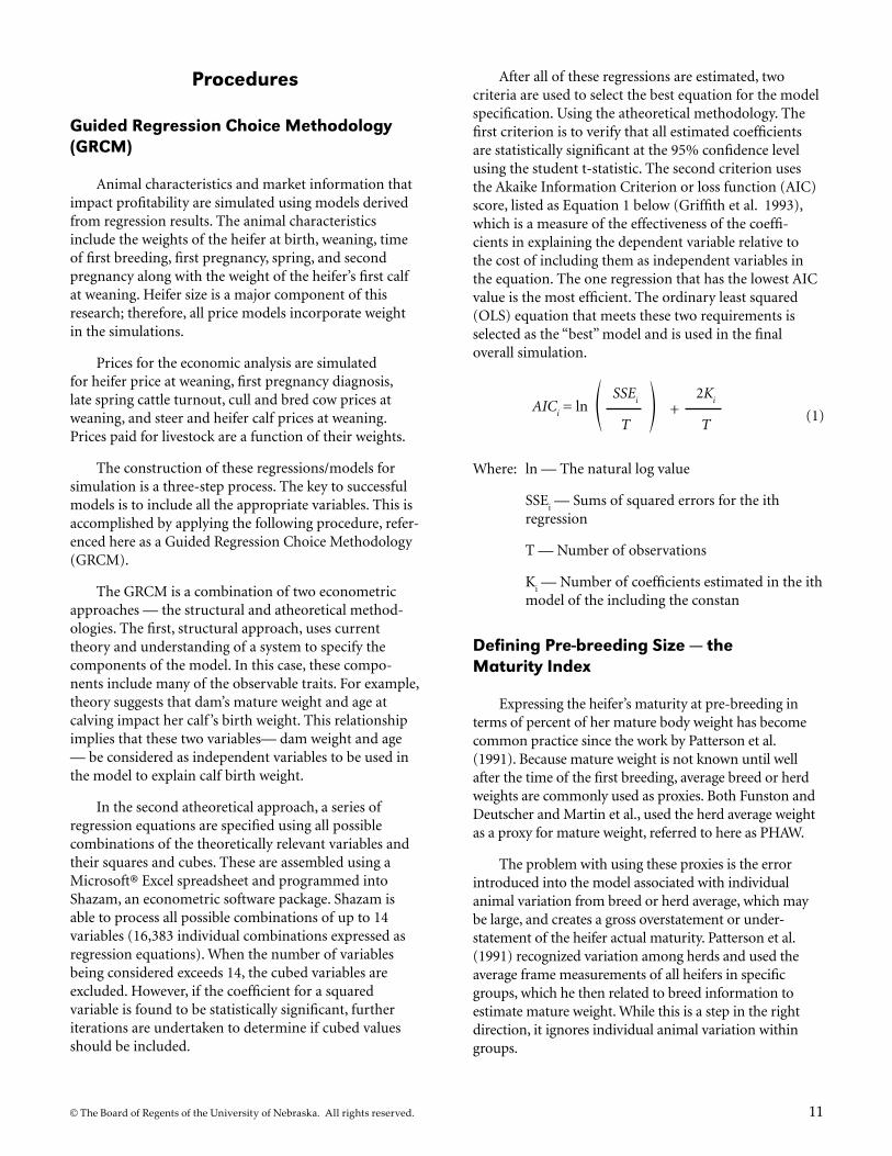
After all of these regressions are estimated, two criteria are used to select the best equation for the model specification. Using the atheoretical methodology. The first criterion is to verify that all estimated coefficients are statistically significant at the 95% confidence level using the student t-statistic. The second criterion uses the Akaike Information Criterion or loss function (AIC) score, listed as Equation 1 below (Griffith et al. 1993), which is a measure of the effectiveness of the coeffi-cients in explaining the dependent variable relative to the cost of including them as independent variables in the equation. The one regression that has the lowest AIC value is the most efficient. The ordinary least squared (OLS) equation that meets these two requirements is selected as the “best” model and is used in the final overall simulation.
AICi = ln
SSEi
T +
2Ki
T(1)
Where: ln — The natural log value
SSEi — Sums of squared errors for the ith
regression
T — Number of observations
Ki — Number of coefficients estimated in the ith
model of the including the constan
Defining Pre-breeding Size — the Maturity Index
Expressing the heifer’s maturity at pre-breeding in terms of percent of her mature body weight has become common practice since the work by Patterson et al. (1991). Because mature weight is not known until well after the time of the first breeding, average breed or herd weights are commonly used as proxies. Both Funston and Deutscher and Martin et al., used the herd average weight as a proxy for mature weight, referred to here as PHAW.
The problem with using these proxies is the error introduced into the model associated with individual animal variation from breed or herd average, which may be large, and creates a gross overstatement or under-statement of the heifer actual maturity. Patterson et al. (1991) recognized variation among herds and used the average frame measurements of all heifers in specific groups, which he then related to breed information to estimate mature weight. While this is a step in the right direction, it ignores individual animal variation within groups.

12 © The Board of Regents of the University of Nebraska. All rights reserved.
MI was developed as an alternative to estimating an individual animal’s PMBW. The MI serves as a forecasting tool, representing a real-time indication of the heifer’s percent of mature weight at the time of breeding. It has the advantage of using information specific to an individual animal that is or can be estimated at the time of heifer selection for retention.
The MI is developed using the GRCM procedure and data from the 302 heifers that reached mature weight in the Funston and Deutscher and Martin et al., studies. Each heifer’s actual PMBW is calculated using the actual weight at the time of the first breeding cycle and her recorded weight at maturity. Animals were considered mature upon the weaning of her third calf in the fall of the fourth year of life. In this case, a heifer born in March 1997 is considered mature at her calf ’s weaning in November 2001, approximately 56 months after her birth.
Independent variables used to calculate MI as deter-mined by the GRCM procedure are the heifer’s birth and weaning weights, her weight and age at the time of first breeding, her dam’s mature weight and dam’s age at the time of her birth, and the feed treatment group to which she is assigned.
The model having the lowest AIC score and with all significant variables, as indicated by the p-values in the parenthesis beneath each coefficient, is enumerated below as Equation 2. Weaning weight is not included in the final model. Those effects are most likely embodied in the characteristics of the dam, birth weight, and pre-breeding weight.
MI = 43.351 + 0.03109WtPb
– 0.1419WtBirth
+ (<0.01) (<0.01) (<0.01)
0.000089Age2Heifer
– 0.01272WtDam
+ 1.756AgeDam
– (<0.01) (<0.01) (<0.03)
0.1448Age2Dam
+ 4.888T1 + 2.645T2 + 2.588T3 (<0.03) (<0.01) (<0.01) (<0.01) (2)
Where: MI – Maturity index
WtPb
— Pre-breeding weight
WtBirth
— Birth weight
AgePb
— Pre-breeding age, (in days)
WtDam
— Mature weight of the heifer’s dam
T1 — Dummy/Indicator variable for the feed treatment group resulting in a traditional group average pre-breeding weight of 58% of herd average
T2 — Dummy/Indicator variable for the feed treatment group resulting in a traditional group average pre-breeding weight of 53% of herd average
T3 — Dummy/Indicator variable for the feed treatment group resulting in a traditional group average pre-breeding weight of 56% of herd average
The Mean Absolute Percent Error (MAPE) procedure, Equation 3, uses within sample data to compare MI forecast with two other methods of deter-mining a heifer’s percent of mature weight.
MAPE =1n Σ n
i=1
| Ai – F
i |
Ai
(3) Where: MAPE — Mean Absolute Percent Error
n — Number of animals used in the test, n = 302
Ai — Heifer’s actual percent mature body weight
at the time of pre-breeding
Fi — Heifer’s forecasted percent mature body
weight at the time of pre-breeding
The first alternative method, PHAW, is described above and is used by Funston and Deutscher (2004) and Martin et al. (2008). The second method uses a more individual approach in that the weight of the heifer’s dam is used as a proxy for a heifer’s mature weight rather than a breed or herd average. This method results in a percent of dam’s mature weight (PDMW). It is expected that PDMW will provide a more accurate measure of maturity relative to the PHAW, and a less accurate measure when compared to the MI.
The predictor with the lowest MAPE is considered the most accurate predictor of the actual percent of mature body weight. The MAPE for MI was the smallest at 5.7% compared to 8.9% for PDMW and 12.3% for PHAW.
As the superior within sample measure of a heifer’s percent of mature body weight, the MI is the measure used for all subsequent analyses.
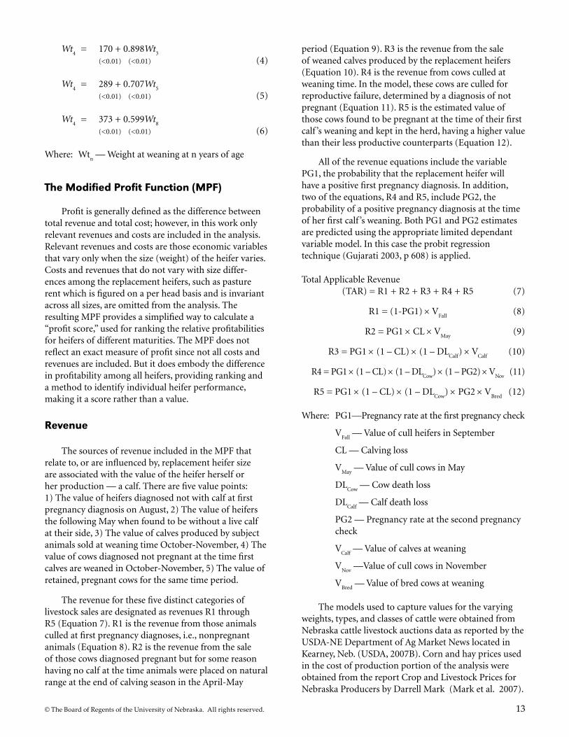
It should be noted that dam mature weight, a component in the MI model, is not available for all dams of the heifers included in this study, necessitating imputation of the missing values. Each heifer’s dam has a recorded weight for at least one of the following years of age: 3, 4, 5, or 8. Forecasting equations were constructed using only dams with known mature weights and the OLS procedure to estimate the missing weights. In each forecasting model, the mature weight at the age of approximately 54 months is the dependent variable and is predicted by weights from one of the other years. Equations 4 through 6 are the resulting equations. The number in parentheses beneath each coefficient is the p-value obtained from performing a student t-test. All are highly statistically significant.
© The Board of Regents of the University of Nebraska. All rights reserved. 13
Wt4 = 170 + 0.898Wt
3
(<0.01) (<0.01) (4)
Wt4 = 289 + 0.707Wt
5
(<0.01) (<0.01) (5)
Wt4 = 373 + 0.599Wt
8
(<0.01) (<0.01) (6)
Where: Wtn — Weight at weaning at n years of age
The Modified Profit Function (MPF)
Profit is generally defined as the difference between total revenue and total cost; however, in this work only relevant revenues and costs are included in the analysis. Relevant revenues and costs are those economic variables that vary only when the size (weight) of the heifer varies. Costs and revenues that do not vary with size differ-ences among the replacement heifers, such as pasture rent which is figured on a per head basis and is invariant across all sizes, are omitted from the analysis. The resulting MPF provides a simplified way to calculate a “profit score,” used for ranking the relative profitabilities for heifers of different maturities. The MPF does not reflect an exact measure of profit since not all costs and revenues are included. But it does embody the difference in profitability among all heifers, providing ranking and a method to identify individual heifer performance, making it a score rather than a value.
Revenue
The sources of revenue included in the MPF that relate to, or are influenced by, replacement heifer size are associated with the value of the heifer herself or her production — a calf. There are five value points: 1) The value of heifers diagnosed not with calf at first pregnancy diagnosis on August, 2) The value of heifers the following May when found to be without a live calf at their side, 3) The value of calves produced by subject animals sold at weaning time October-November, 4) The value of cows diagnosed not pregnant at the time first calves are weaned in October-November, 5) The value of retained, pregnant cows for the same time period.
The revenue for these five distinct categories of livestock sales are designated as revenues R1 through R5 (Equation 7). R1 is the revenue from those animals culled at first pregnancy diagnoses, i.e., nonpregnant animals (Equation 8). R2 is the revenue from the sale of those cows diagnosed pregnant but for some reason having no calf at the time animals were placed on natural range at the end of calving season in the April-May
period (Equation 9). R3 is the revenue from the sale of weaned calves produced by the replacement heifers (Equation 10). R4 is the revenue from cows culled at weaning time. In the model, these cows are culled for reproductive failure, determined by a diagnosis of not pregnant (Equation 11). R5 is the estimated value of those cows found to be pregnant at the time of their first calf ’s weaning and kept in the herd, having a higher value than their less productive counterparts (Equation 12).
All of the revenue equations include the variable PG1, the probability that the replacement heifer will have a positive first pregnancy diagnosis. In addition, two of the equations, R4 and R5, include PG2, the probability of a positive pregnancy diagnosis at the time of her first calf ’s weaning. Both PG1 and PG2 estimates are predicted using the appropriate limited dependant variable model. In this case the probit regression technique (Gujarati 2003, p 608) is applied.
Total Applicable Revenue (TAR) = R1 + R2 + R3 + R4 + R5 (7)
R1 = (1-PG1) × VFall
(8)
R2 = PG1 × CL × VMay
(9)
R3 = PG1 × (1 – CL) × (1 – DLCalf
) × VCalf
(10)
R4 = PG1 × (1 – CL) × (1 – DLCow
) × (1 – PG2) × VNov
(11)
R5 = PG1 × (1 – CL) × (1 – DLCow
) × PG2 × VBred
(12)
Where: PG1—Pregnancy rate at the first pregnancy check
VFall
— Value of cull heifers in September
CL — Calving loss
VMay
— Value of cull cows in May
DLCow
— Cow death loss
DLCalf
— Calf death loss
PG2 — Pregnancy rate at the second pregnancy check
VCalf
— Value of calves at weaning
VNov
—Value of cull cows in November
VBred
— Value of bred cows at weaning
The models used to capture values for the varying weights, types, and classes of cattle were obtained from Nebraska cattle livestock auctions data as reported by the USDA-NE Department of Ag Market News located in Kearney, Neb. (USDA, 2007B). Corn and hay prices used in the cost of production portion of the analysis were obtained from the report Crop and Livestock Prices for Nebraska Producers by Darrell Mark (Mark et al. 2007).

14 © The Board of Regents of the University of Nebraska. All rights reserved.
Cattle values and costs for the value and costs points are associated with a base period. For instance, given the year 2003 as the base period: 1) Acquisition cost of the heifers, C1, and the feed cost prior to breeding, C2, are calculated using the November 2002 values and prices, 2) Value of nonpregnant heifers sold as culls, R1, incor-porates the model for fall values using the 2003 infor-mation, 3) R2, the value of heifers that did not have a calf at the end of the calving season, use May 2004 values. 4) R3, weaned calves, R4, nonpregnant cows sold when the first calf crop is weaned, and R5, the value of bred cows that are retained, are all based on the appropriate 2004 information. Each cohort of heifers requires a complete set of prices spanning three years. Only three base years are considered, 2003 through 2005.
Death loss for both calves and cows is assumed to be 2%. The calving loss rate, which includes missed diagnosis, abortions, fetal death, and calf death up to May following parturition, is an estimate made from GSL information. This rate was estimated at 7.4%. The rate is reflective of first-calf heifers and is different for older cows. Calving loss is statistically related to MI, and is held constant across all maturities and sizes.
Cost
Costs that do not vary by heifer size or treatment group are not included in the model to determine relative profitability since to do so would only complicate the math and provide no benefit in the ranking of the various animals. The three costs identified as being associated with maturity differences are purchase cost or value at weaning (C1), individual feeding costs during the development period for the different nutritional groups (C2), and costs associated with dystocia (C3). Other costs attrib-utable to maturity differences are intrinsically included in the pregnancy rates, cull values, and death losses of the animals on the revenue side of the MPF.
Total Applicable Cost (TAC) = C1 + C2 + C3 (13)
C1 = WtWean
× V Wean
(14)
C2 = FeedConsumed
× Cost Feed
(15)
C3 = PG1 × CDRate
× DCalving
(16)
Where: WtWean
— Replacement heifer’s weight at wean-ing
Vwean
— Value of heifer at weaning
FeedConsumed
— Pounds of feed consumed from weaning to first breeding
CostFeed
— Cost per pound of feed fed between weaning and first breeding
PG1 — First pregnancy rate based on maturity (MI)
CDRate
— Estimated rate of calving difficulty, predicted from maturity (MI)
DCalving
— Average cost of a dystocia incident
Pregnancy and Dystocia Rates
Both pregnancy and dystocia results are expressed in the “I” or “z” portion of the probit specification, Equation 18. This portion of the equation looks much like a standard OLS result. The equation is the sum of a vector of coefficients multiplied by their associated independent variables illustrated in Equation 17.
I = c0 + b
1x
1 + b
2x
2 + ... + b
nx
n (17)
Where: c0 — The regression constant
b — the vector of coefficients
x — the vector of independent variables
However, unlike OLS, the probit equation is a nonlinear estimation and is estimated by the maximum likelihood method. Because of its form, the interpre-tation of probit coefficients varies from the typical OLS regression equation. The “I” is the distance in standard deviations from the mean of zero. Equation 18 shows this cumulative distribution functional form, CDF, which is integrated from negative infinity to the specific value of “I”, where “z < I” is the effect of the dependent variables on standard deviations from the normal distri-bution with a mean of 0 and a standard deviation of 1.
The coefficients estimates relate directly to their effect on standard deviations from the mean relative to the magnitude of the dependent variables and indirectly to the probability P
i. A positive coefficient indicates that
corresponding variable has a positive effect on increasing the probability P
i. The opposite is true of a negative
coefficient. An “I” that is linear in coefficients, but quadratic in variables, will have varying effects, given the sign and magnitudes of the coefficient estimates over the range of the data. It is possible to derive an optimal value for a specific x in the presence of certain conditions.
[ ] ( )∫=
∝−=
−−=≤=Iz
z
zii eIzPP 2/2
1 2
2π (18)
The area under any normal distribution is always equal to one, by definition; the use of this modeling procedure will always translate into a value that ranges

© The Board of Regents of the University of Nebraska. All rights reserved. 15
between zero and one, no matter the size of “I”. The estimation is easily accomplished in several econometric software programs using a subroutine package, in this case SHAZAM.
First pregnancy
The pregnancy rate, or probability of a heifer being pregnant at the first pregnancy diagnosis (PG1), is determined using a probit regression as described above. The coefficient estimates for this pregnancy rate is accomplished by estimating the effects of MI and its square on first pregnancy. All heifers were assigned a zero for a negative pregnancy diagnosis and a 1 for a positive pregnancy diagnosis. The squaring of the MI variable allows for the possibility of diminishing effects that maturity might have on pregnancy. Evidence and idealized facts suggest that pregnancy rates level off at some maturity point and decline as heifers become excessively heavy (Patterson et al. 1992). There is also the expectation that not all animals are capable of becoming pregnant, especially in a short window of opportunity. These facts are consistent with the notion of diminishing marginal return; at some point an added unit of input results in less output than the previous added unit of input. A common way to model this phenomenon is with a quadratic function, as applied here.
To verify the relative effectiveness of using MI and MI squared as independent variables in predicting first pregnancy rate, the results are compared to using PHAW and PDMW as independent variables in a series of six probit estimations. First pregnancy is the dependent variable in each regression. Each of the three variables is used singularly, and with their squared value. Each model is then compared using student t-statistics for the coefficient estimates and the Normalized Success Index (NSI) to evaluate their comparative effectiveness.
The NSI is described by Hensher and Johnson (1981) and is one measure of the effectiveness of a probit regression. NSI is the weighted sum of the success indices by their proportional error. In this case, two outcomes are possible: pregnancy or nonpregnancy. The success index for nonpregnancy is the number of correctly predicted nonpregnancies — those heifers whose pregnancy prediction is below the average pregnancy rate for the group (90.141%) divided by the number of heifers predicted to be nonpregnant, minus the ratio of those predicted to be pregnant as a proportion of the total number of heifers. The success index for pregnancy is calculated similarly with the appropriate measures. The higher the NSI value, the better the fit
of the regression equation. Further explanation of the NSI is available in the Shazam User’s Reference Manual (Whistler et al. 2007, pp 296-297).
Table 1 shows the results of both the student t-statistic and the NSI scores for each of the six different equation specifications.
Table 1. Comparison of independent variables in the rate of first pregnancy probit results
Independent Variable(s)
p-values
ConstantLinear Coef.
Squared Coef. NSI
PHAW .89 .14 — .032
PDMW .59 .13 — .030
MI .77 .18 — .025
PHAW and PHAW squared .11 .08 .10 .089
PDMW and PDMW squared .44 .31 .38 .090
MI and MI squared .03 .03 .04 .092
The regression using MI in the quadratic form results in the only probit with statistically significant coefficient estimates. It is also the only statistically signif-icant overall equation using the Log Likelihood Ratio Test, and an Xi square with k-1 degrees of freedom.
In a comparison of predictive performance of the quadratic models only, the MI Squared model overpre-dicts nonpregnancy fewer times than the other two competing models with PDMW, the model that uses mature dam weight and predicts the most nonpreg-nancies. In predicting pregnancy, the same pattern of performance is repeated, with the MI having the least errors followed by PHAW, the herd average model, and lastly PDMW, the mature dam weight model. All three models have less error in predicating pregnancy versus nonpregnancy, with predicted shares of MI, 71%; PHAW, 70%; and PDMW, 64% (see Appendix 1, NSI Tables for complete details).
Equation 19 shows the coefficient estimates and their associated p-values for the MI and MI squared probit model.

16 © The Board of Regents of the University of Nebraska. All rights reserved.
IPG1
= –28.372 + 0.959MI – .00756MI2
(0.03) (0.03) (0.04) (19)
Where: IPG1
— Distance from its mean, 0, in standard deviations, assuming a ~N(0,1) distribution
MI —Maturity Index, measure of maturity
Dystocia
Once a heifer is diagnosed pregnant, the next major event in her life and in the production process is partu-rition, or calving. A major cost and concern with calving heifers is whether or not they will have difficulty during the parturition process. Difficulty creates cost and may affect further productivity, fertility, and health. The technical term for calving difficulty is dystocia. Maturity or MI is expected to be inversely related to dystocia. As maturity increases, the likelihood of dystocia is thought to decrease.
Patterson et al. (1991) suggests that heifers that are smaller at calving “experienced a higher incidence of calving problems. ” To test this hypothesis, a series of probit regression equations were estimated using the results of the pregnancy diagnoses at the time of the first calf ’s weaning as the dependent variable, and the absence or presence of dystocia as the independent variable being assigned a value of zero or one respectively. Dystocia is present if a heifer required any aid in giving birth.
Seven probit models are compared using the student t-statistic and the NSI. Of the seven, only three have statistically significant coefficients: linear, quadratic, and cubic variable specifications. The results of the estimation process for these three are documented in Equations 20-22. The quadratic and cubic forms are introduced with the expectation that they provide diminishing marginal return effects.
ID1
= 3.559 – 0.0689 MI (<0.01) (<0.01) (20)
ID2
= 1.504 – 0.000575 MI2
(<0.01) (<0.01) (21)
ID3
= .816 – 0.00000636 MI3
(<0.04) (0.01) (22)
Where: I
Di , i = {1, 2, 3} — Distance the value is from its
mean, assuming a ~N(0,1) distribution
MI — Maturity Index, measure of maturity
Each of the coefficient estimates is statistically significant for each of the three forms. The ranking of the three models using NSI is described in Table 2. The linear form has the largest NSI value, giving it a superior rank over the other two models; thus, it is the model of choice. Please note that these models are only valid over the range of the data from which they are created. Caution should always be practiced when predictions lie outside the practical limits of the data.
Table 2. Normalized Success Index (NSI) for Dystocia Using Three Different Forms of MI
Form of MI Normalized Success Index
Linear 0.0592
Quadratic 0.0588
Cubic 0.0533
Equations 20-22 in combination with Equation 18 are used to calculate the dystocia rates for MI scores that range from 50 to 73, the range of MI scores observed in the data. The results of these calculations are graphed in Figure 1. This provides insight into the effect of the different model forms and makes a good visual comparison. The predicted probabilities of dystocia as predicated by the three different functions are listed in Appendix 2.
Surprisingly the linear form of the dystocia probit shows the most curvature. This, at first, may seem counterintuitive — a linear model generally reflects a straight line. In this case, the curvature is not related to the linear nature of the I, but is the result of the trans-lation of the linear I into P
i by the exponential equation
of the normal CDF. This linear form of the probit model shows a dystocia rate of more than 50% for heifers with an MI of 50, and less than 10% for the more mature heifers with MI scores above 70. The shallowing slope of the linear probit curve indicates that maturity is having a diminished effect on dystocia with increasing MI scores. This outcome is consistent with expectations. Logically, dystocia is likely to occur at some rate regardless of the level of maturity.
Second pregnancy
Each specific MI is translated into a first pregnancy rate, PG1, and a dystocia rate D, using the appropriate estimated equations. Each specific heifer’s rate of dystocia and first pregnancy are expressed as a probability based on her maturity. The estimated

© The Board of Regents of the University of Nebraska. All rights reserved. 17
relationships predict heifers with an MI score of 60 to have a 97.5% chance of being diagnosed pregnant with their first pregnancy diagnosis and, if diagnosed pregnant, a 28% chance of having dystocia. This compares to a heifer with a MI score of 50 having a 75.1% chance of being diagnosed pregnant and a 54.5% chance of having dystocia.
The next logical step is to determine the factors that affect second pregnancy. The model for estimating second pregnancy rate, PG2, is derived using the probit specification. However, unlike first pregnancy rates, dystocia, not MI, is found to be the statistically signif-icant driver. None of the models created using MI as a dependent variable have statistical significance at the 95% level of confidence.
The probit regression shows the relationship between dystocia at first calving and successful rebreeding to be negative and statistically significant (Equation 23). The results expressed in Equation 23, I
PG2,
must be translated through Equation 18 to be interpreted as the second pregnancy rate, PG2. This translation
shows the rate of a second pregnancy for a cow that exhibits dystocia during first parturition to be 84.31% versus 94.98% if she does not, a decrease in fertility of about 10%.
IPG2
= 1.645 – 0.637 D (<0.01) (<0.01) (23)
Where: IPG2
– Distance the value is from its mean, assuming a ~N(0,1) distribution
D – Variable indicating the presence of dystocia
Unlike the previous two probit models, the right-hand side variable is a condition or choice variable, represented by a zero or one. This choice variable is interpreted as a single occurrence with a discrete one-time effect on the second pregnancy rate. Unfortu-nately, this fact makes this equation an unusable input into the profit function since it forecasts the effects of dystocia only with actual knowledge. Operationally, what is needed is a method of estimating second pregnancy rate based on continuous probabilities of dystocia.
Figure 1. Predicted dystocia rates as forecast by maturity index measures using three different probit specifications for I
Pro
ba
bili
ty o
f D
ysto
cia
0.50
0.40
0.30
0.20
0.10
0.00
50 55 60 65 70
Maturity Index
CubedLinear Squared

18 © The Board of Regents of the University of Nebraska. All rights reserved.
Two methods are considered here to accomplish this purpose. The first method is to use the parameter estimates from Equation 23, with the predicted dystocia values from Equation 20 to estimate rates for second pregnancy. Remember that these predicted values for dystocia are the result of using the MIs in Equation 20, translated through Equation 18, a normal CDF. This method results in small variation in expected second pregnancy rates, with a range from 94.31% to 90.78%, (Figure 2), which is not consistent with the range in probabilities of second pregnancy observed in the data.
The second method re-estimates Equation 23 using predicted dystocia from Equation 20 and 18, creating the continuous variable needed to make a continuous forecast from the MI prior to the event occurring. This methodology yields Equation 24, with coefficient estimates results not unlike Equation 23 above.
ˆIPG2
= 1.8531 – 0.0165 Dc
(<0.01) (<0.01) (24)
Where: IPG2
– Distance the value is from its mean, assuming a ~N(0,1) distribution
Dc– A continuous variable for dystocia,
predicte d by MI using Equation 20 and 18
The range of predictions for second pregnancy using Equation 24 is more consistent with the observed range of 84.95% to 95.49%. Both the first and second method outcomes are illustrated in Figures 2 and 3. Figure 2 shows the relationships between MI and second pregnancy using both methods, while Figure 3 shows the relationships between Dystocia and second pregnancy.
Pro
ba
bili
ty o
f S
eco
nd
Pre
gn
an
cy
98%
96%
94%
92%
90%
88%
86%
84%
50 55 60 65 70
Maturity Index
Method 1: Predicted Second Pregnancy Using Actual Probit and Predicted Dystocia RatesMethod 2: Predicted Second Pregnancy Using Probit From Predicted Dystocia Rates
Figure 2. Estimated second pregnancy rates as a function of the maturity index

© The Board of Regents of the University of Nebraska. All rights reserved. 19
In addition to this visual comparison, an NSI is used to compare the difference in the two methods’ overall accuracy of predicting second pregnancy correctly. The raw NSI tables are found in Appendix 3, with a summary in Table 3.
Table 3 shows some interesting differences between the two methods. Both methods have statistical signifi-cance for all parameters at the 95% level; however, Method 2 loses statistical significance for its slope term if significance is set above the 96% confidence level. Method 2 has a higher NSI score (see Appendix 4 for the raw tables and details of the scoring). Method 2 has two advantages for use in this study. First, the stream of information flows in a continuous flow, and second, the range of outcomes more closely matches that of the
existing data. For these reasons, Method 2 is used to create the final MPF.
Table 3. Comparison of the methods used for estimating maturity’s effect on second pregnancy
Statistically Significant NSI Scores
Method 1 yes 0.046
Method 2 yes 0.066
Figure 3. Estimated second pregnancy rates as a function of dystocia rate
Pro
ba
bili
ty o
f S
eco
nd
Pre
gn
an
cy
98%
96%
94%
92%
90%
88%
86%
84% 0% 10% 20% 30% 40% 50% 60%
Probability of Dystocia
Method 1: Predicted Second Pregnancy Using Binary Data Probit and Predicted Dystocia RatesMethod 2: Predicted Second Pregnancy Using Probit Created From Predicted Dystocia Rates

20 © The Board of Regents of the University of Nebraska. All rights reserved.
Revenue Equation Specifics
Revenue 1 (R1)
In addition to PG1, the R1 revenue equation includes the value of heifers diagnosed as nonpregnant at first pregnancy diagnosis in the fall (V
Fall). Culled,
nonpregnant heifers are sold as feeder cattle, so their values are calculated using feeder calf prices for the month of September.
Feeder calf value is a product of weight and price, where price per pound is on a “slide,” per pound prices diminishing as weight increases. Other factors that alter price include gender and seasonal fluctuations. Heifer calves are generally sold at a discount relative to steer calves, and winter and spring calves sell at a premium relative to fall calves. All of these relationships are intrinsically imbedded in the price information used to estimate value.
As in real life, the sale weight must be known before the value can be determined. Equation 25 is the model identified by the GRCM procedure used to predict the weights of nonpregnant heifers. The student t p-values of each coefficient are in parentheses below each estimate.
WtFall
= 388.8 – 2.47 × 10⁻⁵ Wt3Birth
+ 2.05 × 10⁻⁷ Wt3Wean
+ (<0.01) (0.03) (0.02)
1.98×10⁻³ Wt2Pb
– 1.48 × 10⁻⁶ Wt3Pb
– 23.26T1 – (<0.01) (<0.01) (<0.01)
16.33T2 – 27.17T3 (<0.01) (<0.01) (25)
Where: Wt
Fall — Predicted weight at first pregnancy
diagnosis (dependent variable)
WtBirth
— Birth weight
WtWean
— Weaning weight
WtPb
— Pre-breeding weight
T1 — Dummy variable for feeding treatment group resulting in a pre-breeding weight of 58% of mature body weight
T2 — Dummy variable for feeding treatment group resulting in a pre-breeding weight of 53% of mature body weight
T3 — Dummy variable for feeding treatment group resulting in a pre-breeding weight of 56% of mature body weight
The signs and magnitudes of the estimated coefficients are consistent with expectations. Pre-breeding weight, Wt
Pb, birth weight, Wt
Birth, and
weaning weight, WtWean
, each have a positive association with fall weight, Wt
Fall. Larger animals tend to stay
larger from birth to fall sale. At first glance the indicator variables accounting for pre-breeding nutrition seem to conflict with expectations, but they are easily understood using the premise of compensatory gains. Compensatory gain is the commonly observed phenomenon where growing animals that have received a lower nutritional level during one phase of growth tend to make up for the difference if given adequate nutrition during a later phase of growth. The higher plane of nutrition makes for a heavier animal at pre-breeding, but other genetically similar animals grow compensatorily when put on good pasture during the breeding period, making heifers in a treatment group with higher levels of nutrition and a corresponding higher level of pre-breeding weight, gain about 16 to 27 pounds less between pre-breeding and fall sale.
The price data used to predict fall sale value, VFall
, are provided by the Nebraska livestock auction markets recorded by the USDA AMS (Agricultural Marketing Service), and are listed as average weights and prices by week for groups of cattle. Heifer prices for the last two weeks in September and the first two weeks in August for years 2000 through 2007 are the actual series used.
An OLS regression is used to determine the relationship between value per head and weight at the first pregnancy diagnosis (Wt
Fall). Value per head
(VFall
) is the dependent variable; forecast weight at first
pregnancy diagnosis (WtFall
) and eight indicator variables that account for yearly differences are the independent variables. The coefficient estimates with their respective p-values in parentheses are below in Equation 26.
VFall
= 253.56 + 0.67WtFall
+ 5.51Yr2001
– 89.13Yr2002
+ (<0.01) (<0.01) (0.20) (<0.01)
67.44Yr2003
+ 174.67Yr2004
+ 118.87Yr2005
+ (<0.01) (<0.01) (<0.01)
108.83Yr2006
+ 93.50Yr2007
(<0.01) (<0.01) (26)
Where: VFall
= Cull heifer’s per head value
WtFall
— Weight at first pregnancy check
Yrn — Dummy variable for year n

© The Board of Regents of the University of Nebraska. All rights reserved. 21
This relationship estimates individual heifer’s value as $253.56 plus 67% of the fall weight (Wt
Fall) in pounds,
plus an annual market correction factor by year. The year 2000 is the base year, so it adjusts the fall value by zero dollars. Years other than 2000 have a correction value. The year 2002 has a negative correction value of nearly $90.00 per head, while the year 2004 has a positive correction of over $174 per head. The year 2001 is not statistically different from the base year, using a 95% confidence level. These results are indicative of how the cattle market fluctuates from year to year.
Revenue 2 (R2)
The R2 revenue (Equation 8) estimates the value of those replacement females culled after the calving season and prior to release onto native range. As with R1, this equation includes PG1, with the addition of calving loss (CL), and cull cow values in May (V
May).
The CL rate was not found to be statistically affected by the MI or other cow characteristics at the 95% confi-dence level. CL is estimated from GSL records as the average calf loss for all heifers between the years 2002 and 2007 at 7.4%. This estimate is obtained by taking the number of heifers without calves at the end of the calving period divided by the total number of heifers diagnosed as pregnant in the previous fall, multiplied by 100. The resulting 7.4% is an arithmetic average of the annual CL rates.
Spring birthing cows at GSL calve before the end of April and are put out on native range in May. Calving season is officially over with the move to native range. Heifers culled at this stage of production are not sellable as feeder cattle, since they are too old and are larger than what is considered ideal for feeder animals. It is conceivable that these cows could receive some type of premium at sale, but for purposes of this work, we have ignored this possibility and leave it for future investi-gation. These animals are sold as utility grade cull cows. Prices for all cull cows in this study were obtained from the Livestock Market Information Center (LMIC) and are from numerous reports from the USDA-AMS for the Sioux Falls, S.D., auction market (Livestock Market Information Service 2010). Unlike feeder animals, there is no price slide for utility grade animals. May utility cow prices are used to calculate V
May and need no adjustment
since cows have no slide or other adjustment. The value of the cull animals, V
May,, is the product of the average
May utility cow price for the appropriate year, times their estimated weight in May (Wt
May).
The GRCM procedure was used to create the model for predicting May weights, Equation 27.
WtMay
= –371.73 + 0.0453WtDam
+ 0.687WtBirth
+ (0.05) (<0.01) (<0.01)
0.000325Wt2Pb
+ 1.879WtPG1
– 0.000785Wt2PG1
– 28.646T1 (<0.01) (<0.01) (<0.01) (<0.01)
– 13.231T2 – 9.987T3 (<0.01) (0.01) (27)
Where: WtMay
— Weight at the end of the calving season
WtDam
— Dam’s mature weight
WtBirth
— Heifer birth weight
WtPb
— Pre-breeding weight
WtPG1
— Weight at first pregnancy diagnosis
T1 — Dummy variable for feeding treatment group resulting in a pre-breeding weight of 58% of mature body weight
T2 — Dummy variable for feeding treatment group resulting in a pre-breeding weight of 53% of mature body weight
T3 — Dummy variable for feeding treatment group resulting in a pre-breeding weight of 56% of mature body weight
The dependent variable, May weight (WtMay
), was unmeasured in the GSL records so a proxy weight is imputed. Since the May weight time period is about halfway between the time when fall weight and second pregnancy weights are recorded, these two events are arithmetically averaged shown in Equation 28.
Wt May
= Wt
Fall + Wt
PG2
2 (28)
Where: WtMay
— Weight at the end of the calving season
WtFall
— Weight at first pregnancy diagnoses
WtPG2
— Weight at second pregnancy diagnoses
Equation 27 forecasts weights based on five factors: dam’s weight, birth weight, pre-breeding weight, weight at first pregnancy diagnosis, and nutrition level. For every 100 pounds of dam weight, the May weight increases by 4½ pounds. Every pound of birth weight increases May weight by .687 pounds. Pre-breeding weight has an effect that increases at an increasing rate, with an average increase of 1.625 pounds for every 50 pounds of pre-breeding weight over the weight range of the breeding weights considered here. Fall weight at first pregnancy diagnosis has a quadratic relationship to May weight. First pregnancy weights up to 1196.82 pounds increase May weight, and those greater than that
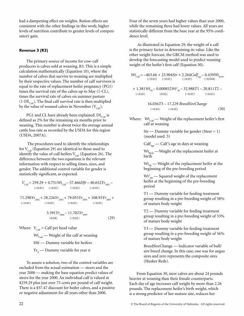
22 © The Board of Regents of the University of Nebraska. All rights reserved.
had a dampening effect on weights. Ration effects are consistent with the other findings in this work; higher levels of nutrition contribute to greater levels of compen-satory gain.
Revenue 3 (R3)
The primary source of income for cow-calf producers is calves sold at weaning, R3. This is a simple calculation mathematically (Equation 10), where the number of calves that survive to weaning are multiplied by their respective values. The number of calf survivors is equal to the rate of replacement heifer pregnancy (PG1) times the survival rate of the calves up to May (1-CL), times the survival rate of calves on summer pasture (1-DL
Calf). The final calf survival rate is then multiplied
by the value of weaned calves in November (VCalf
).
PG1 and CL have already been explained. DLCalf
is defined as 2% for the remaining six months prior to weaning. This number is about twice the average annual cattle loss rate as recorded by the USDA for this region (USDA, 2007A).
The procedures used to identify the relationships for V
Calf (Equation 29) are identical to those used to
identify the value of cull heifers VFall
(Equation 26). The difference between the two equations is the relevant information with respect to selling times, sizes, and gender. The additional control variable for gender is statistically significant, as expected.
VCalf
= 259.29 + 0.751WtCalf
– 57.466Hfr – 40.652Yr2001
– (<0.01) (<0.01) (<0.01) (<0.01)
71.298Yr2002
+ 28.226Yr2003
+ 79.055Yr2004
+ 108.93Yr2005
+ (<0.01) (<0.01) (<0.01) (<0.01)
5.591Yr2006
– 11.702Yr2007
(0.04) (<0.01) (29) Where: V
Calf = Calf per head value
WtCalf
— Weight of the calf at weaning
Hfr — Dummy variable for heifers
Yrn — Dummy variable for year n
To assure a solution, two of the control variables are excluded from the actual estimation — steers and the year 2000 — making the base equation predict values of steers for the year 2000. An individual calf is valued at $259.29 plus just over 75 cents per pound of calf weight. There is a $57.47 discount for heifer calves, and a positive or negative adjustment for all years other than 2000.
Four of the seven years had higher values than year 2000, while the remaining three had lower values. All years are statistically different from the base year at the 95% confi-dence level.
As illustrated in Equation 29, the weight of a calf is the primary factor in determining its value. Like the other weight forecast, the GRCM method was used to develop the forecasting model used to predict weaning weight of the heifer’s first calf (Equation 30).
WtCalf
= –463.66 + 23.904Str + 2.264CalfAge
– 0.439WtBirth
(<0.01) (<0.01) (<0.01) (<0.044)
+ 1.381WtPb
– 0.000852Wt2Pb
– 32.988T1 – 20.811T2 – (<0.01) (0.02) (<0.01) (<0.01)
16.036T3 – 17.229 BreedSireChange (<0.01) (<0.01) (30)
Where: WtCalf
— Weight of the replacement heifer’s first calf at weaning
Str — Dummy variable for gender (Steer = 1) (model used .5)
CalfAge
— Calf ’s age in days at weaning
WtBirth
—Weight of the replacement heifer at birth
WtPB
— Weight of the replacement heifer at the beginning of the pre-breeding period
Wt2PB
— Squared weight of the replacement heifer at the beginning of the pre-breeding period
T1 — Dummy variable for feeding treatment group resulting in a pre-breeding weight of 58% of mature body weight
T2 — Dummy variable for feeding treatment group resulting in a pre-breeding weight of 53% of mature body weight
T3 — Dummy variable for feeding treatment group resulting in a pre-breeding weight of 56% of mature body weight
BreedSireChange — Indicator variable of bull/sire breed change. In this case, one was for angus sires and zero represents the composite sires (Husker Reds).
From Equation 30, steer calves are about 24 pounds
heavier at weaning than their female counterparts. Each day of age increases calf weight by more than 2.26 pounds. The replacement heifer’s birth weight, which is a strong predictor of her mature size, reduces her

© The Board of Regents of the University of Nebraska. All rights reserved. 23
offspring’s weaning weight by nearly 0.44 pounds. This decrease in a heifer offspring’s weaning weight is partially offset by the calf ’s gain from her pre-breeding weight. Heifers that are heavier at birth are generally heavier at pre-breeding (Equation 39). Replacement heifers in this study ranged from 420 to 854 pounds at pre-breeding. Higher levels of heifer nutrition directly decrease first calf ’s weaning weight for animals of the same size at pre-breeding but may not for animals that are genetically larger. These negative numbers in effect compenstate for animal growth. The nutrition effect ranges from just over 16 to over a 33-pound reduction in calf weaning weight. The breed sire change variable (BreedSireChange) reflects a change in offspring genetics that occurred in the operation at GSL during the time of the studies. Heifers were bred to Angus bulls through the 2002 breeding season. Beginning in the 2003 breeding season, heifers were bred to Husker Red bulls. This variable is used to control for any differences this practice created. The magnitude of this coefficient estimate indicate that calves born to the Black Angus sires are 17 pounds lighter at weaning than those born to the Husker Red sires.
Several facts about Equation 30 are worthy of note. Each added day of calf age increases weaning weight by ~ 2.26 pounds. However, through the use of an AIC method, calf age is found to have a second order polynomial relationship with the dam’s maturity at breeding (Equation 31).
CalfAge
= 147.1+9.958 MI – .076193 MI2
(0.25) (0.025) (0.017) (31)
Where: CalfAge
— Calf ’s age in days at weaning
MI — Maturity Index, measure of maturity
MI2 — Squared maturity index
This equation predicts that a replacement female with an MI score of 50 at pre-breeding is expected to wean a calf of about 160.4 days of age. This is 18 days younger than the expected age at weaning of 178.4 days for a calf born to a heifer with a MI score of 65.34, the optimal score to produce the oldest weaned offspring; forecast.
Figure 4. Maturity index as a predictor of age of heifer’s first calf at weaning
Ag
e in
Da
ys o
f Fi
rst
Ca
lf a
t W
ean
ing
208
198
188
178
168
158
148
13851 56 61 66 71
Maturity Index
Actual Age of CalfPredict Age of Calf

24 © The Board of Regents of the University of Nebraska. All rights reserved.
Actual ages and those predicted by the quadratic MI equation for the replacement heifers are illustrated in Figure 4.
With the number of positive and negative effects of the various factors that contribute to the replacement heifer calf ’s weaning weight, it is difficult to identify the overall outcome without considerable calculation. The following example is provided to help clarify the individual effects on the final outcome.
Consider two replacement heifers born the same date (416 days prior to pre-breeding), having the same birth weight (83 pounds) and weaning weight (473 pounds), from dam’s with the identical characteristics of a 1,200 pound mature weight and 4 years of age. Using Equations 39 and 40, if one of these heifers is fed at a higher rate of nutrition relative to the other — in this case T1 (high) versus T4 (low)— the estimated difference in weight between the two animals at pre-breeding is approximately 108 pounds (from Equaiton 41) (685 pounds for the animal receiving the T1 ration compared to 577 pounds for the animal receiving the T4 ration). The MI of the heavier animal would be 62.59, while that of the smaller animal would be 54.36 (Equation 2). Using the relationships from Equations 30 and 31, the heifer’s added pre-breeding weight from the higher energy diet results in her first calf being just over 19 pounds heavier at weaning than the first calf from the heifer developed on the lower energy ration.
Equation 30 calculates that the T1-developed heifer’s heavier pre-breeding weight adds an additional 32.83 pounds of weaning weight, but this apparent gain is offset by a negative 32.98 pound adjustment for the higher nutritional rate prior to pre-breeding. With the inclusion of the Equation 31 information, the higher MI, created by the higher plain of nutrition, results in an older calf at weaning (8.62 days), adding an additional 19.52 pounds to the weaning weight of her calf. These interactions result in a 19.3 pound weight advantage for the calf born to the heifer fed the higher nutrient ration, T1.
In the application of the model, it is expected that half the animals are male and the other half female. Effectually, this is accomplished using one-half of the coefficient’s value for gender, the variable titled Strs in Equation 30, for every calf.
Revenue 4 (R4)
Revenue R4 (Equation 11) is used to estimate the revenue from the sale of cows that are not pregnant at the time of their second pregnancy diagnoses. It includes: 1) PG1, first pregnancy rate; 2) CL calf loss and unborn
rate, making 1-CL the percent of live calves at cows’ side just prior to spring range turnout; 3) DL
Cow, death loss
for cows, and 1- DLCow
, percent of live cows; 4) PG2, pregnancy rate determined by the second pregnancy diagnoses at first calf weaning, with 1- PG2 percent of cows found not to be pregnant; and 5) V
Nov, value of
nonpregnant cows for the month of November. The DL
Cow information obtained was held at an annual rate
of 2%, consistent with the data from the USDA report (USDA, 2007A).
The relationships between MI and second pregnancy diagnosis are incorporated into R4 indirectly through the dystocia and second pregnancy relationship. Equation 20 captures the statistical relationship between MI and dystocia, and Equation 24 describes the relationship between the probability of dystocia and second pregnancy, with the probability of dystocia expressed as a decimal between zero and one. Equation 24 provides the means to apply the information gained from Equation 20, where MI is used to predict dystocia rates. Without Equation 24, predictions regarding second pregnancy rates could not be made, since second pregnancy is not directly a function of the MI.
The model for predicting November weight, at the first calf ’s weaning, is created using the GRCM method and is represented in Equation 32.
WtNov
= –743.46+0.0906WtDam
+ 1.373WtBirth
+ (0.05) (<0.01) (<0.01)
0.000650Wt2Pb
+ 2.759WtPG1
– 0.00157Wt2PG1
– 57.291T1 – (<0.01) (<0.01) (<0.01) (<0.01)
26.461T2 – 19.973T3 (<0.01) (<0.01) (32)
Where: WtNov
— Cows Weight at first calf ’s weaning
WtDam
— Dam’s mature weight
WtBirth
— Replacement heifer birth weight
WtPb
— Replacement heifer pre-breeding weight
WtPG1
— Weight at first pregnancy diagnosis, ap-proximately one year previous
T1 — Dummy variable for feeding treatment group resulting in a pre-breeding weight of 58% of mature body weight
T2 —Dummy variable for feeding treatment group resulting in a pre-breeding weight of 53% of mature body weight
T3 — Dummy variable for feeding treatment group resulting in a pre-breeding weight of 56% of mature body weight

© The Board of Regents of the University of Nebraska. All rights reserved. 25
The product of WtNov
and the November cull cow price equals V
Nov. Unlike some of the other classes of
livestock, such as feeder cattle where price is a function of weight and gender, the cull cow classification has no distinction among sizes or gender. Given this simpler relationship, prices are assigned without a slide or gender adjustment factor.
Revenue 5 (R5)
Equation 12, R5, is the final revenue source, the value of 3-year-old pregnant cows. These are the animals that are to be retained in the herd for continued production. Since these cows are pregnant and have a high probability of continued productivity, they are valued at a premium relative to those animals that are culled. The factors for estimating the rate of cows diagnosed pregnant, PG2, is equal to the inverse of 1-PG2, the forecast rate of replacement cows diagnosed as nonpregnant (Equations 18, 20, and 24). The pregnant cows are valued on a per head basis using a model derived from the analysis of data reported by USDA for the Nebraska Livestock Market Auction (USDA, 2007B) and CattleFax, an organization based in Centennial, Colo., that collects and analyzes data relating to the cattle industry. Data collected from the Nebraska auction markets contained information about bred-cow sales for years 2006 and 2007 only.
The model identified by GRCM, using this infor-mation, is encapsulated in Equation 33. This model includes variables for cow weight and two age classes. This model was selected from seven possible models.
VBred (ij)
= 394.49 – 518.25 AgedGroup(i)
– 357.11 MAgedGroup(i)
+ (<0.01) (<0.01) (<0.01)
.68546 AvgWtGroup (i)
(<0.01) (33)
Where: VBred(ij)
— The average value of the (ith) group of cows with no adjustment for year
AgedGroup(i)
— Control variable for the (ith) cow group over 8 years of age
MAgedGroup(i)
— Control variable for the (ith) cow groups more than 3 and less than 9 years of age
AvgWtbGroup(i)
— Average cow group weight, for the ith group of cows
Under normal conditions, Equation 33 would be the model selected to predict the value of bred cows. However, the second best model included coefficient estimates for the 2006 and 2007 market years that were
not statistically different. The expectation, however, is that price differences between 2006 and other years will be different. For this reason, Equation 34 is the model of choice.
Equation 34 includes variables: 1) A control for aged cows (older than 8 years of age), 2) A control variable for middle-aged cows (5 through 8 years of age), 3) Cow weights, and 4) A control variable for 2007. The base equation assumes that cows are young (3 or 4 years of age) with 2006 sale value.
VBred(ij)
= 417.05 – 507.47 AgedGroup(i)
– 344.18 MAgedGroup(i)
+ (<0.01) (<0.01) (<0.01)
.64761 AvgWtGroup(i)
+ 29.70 Year
ij
(<0.01) (0.23) (34)
Where: VBred(ij)
— The average value of the (ith) group of cows in the (jth) year
AgedGroup(i)
— Control variable for the (ith) cow group over 8 years of age
MAgedGroup(i)
— Control variable for the (ith) cow groups more than 3 and less than 9 years of age
AvgWtbGroup(i)
— Average cow group weight, for the ith group of cows
Yearij – Control variable for the (ith) group and
the (jth) year
Cows older than 8 years of age, AgedGroup(i)
, on average receive a $507.47 discount per head relative to 3 and 4 year old cows. Middle-aged cows (MAged
Group(i)), 5 to 8 years of
age, are discounted by $344.18 per head. For any given age classification, a cow’s average value per head increases by nearly $0.65 per pound of body weight. Average cow value increased by $29.70 from 2006 to 2007.
The Nebraska livestock auction markets only contain cow price data for 2006 and 2007 market years. CattleFax monthly average prices for bred cow data are available that provide the information to calculate the four month average price differences for the months of August, September, October, and November by year, Year
(j), for
multiple years including the years of 2000 through 2007. These data were used to derive a model for making annual bred cow price adjustments (Table 4). The base year, 2006, is omitted from the table.
Notice that the CattleFax data estimate the price difference between 2006 and 2007 as $29.69, nearly identical to that estimated by the Nebraska livestock auction market data. With this fact, the assumption is made that price differences from the CattleFax data for

26 © The Board of Regents of the University of Nebraska. All rights reserved.
any of the other years may be substituted for the coeffi-cient estimate of Year
j in Equation 34. This provides a
method to adjust annual differences in bred cow values annually for the missing years of the USDA data.
Cost 1 (C1)
C1, Equation 14, predicts the heifer’s value at the time of her weaning (V
Wean) and represents the cost of
acquiring her as a replacement. For those heifers that are retained as replacements from the productive herd, there is an opportunity cost — the forgone revenue resulting from retaining them rather than selling them at market. This value, like the sales value of calves in R3, depends on the heifer’s size/weight. Smaller heifers are worth more per pound, but the added weight of larger animals usually more than offsets the price. This again is the price slide effect.
Identifying heifer value, VWean
, is a two stage process: 1) Determining a weaning weight and 2) Arriving at a price for heifers of that weight. The function used to predict weight at weaning (Wt
wean) is developed using
GRCM methodology and is found to be a function of the heifer’s birth weight and age cubed, and her dam’s age and age squared (Equation 35).
WtWean
= 235.23 + 1.44WtBirth
+ 1.07 × 10⁻⁵ Age3Wean
+ (<0.01) (<0.01) (<0.01)
1.30 Age2Dam
– 0.0993 Age3Dam
(<0.01) (<0.01) (35)
Where: WtWean
— Weaning weight of replacement heifer
WtBirth
— Birth weight of replacement heifer is predicted with Equation 39
AgeWean
— Age in days of replacement heifer at weaning
AgeDam
— Age of dam at calving
Weaning weight is increased by 1.44 pounds for every pound of birth weight, resulting in a 10 pound difference at birth becoming an additional 14.4 pounds at weaning. The interesting effect due to the cubic variable specifi-cation for heifer age in Equation 35 is increasing age of the heifer at weaning results in increased weaning weight at an increasing rate. At 164 days, the predicted additional weight at weaning due to heifer age is about 0.86 pounds for every day of age. This increases to 1.13 pounds for each day of age at 188 days. A heifer’s dam’s age is expressed as a second-order polynomial, where weaning weight of the calf is maximized when the dam is between 8 and 9 years. The difference between having a 3- year-old dam versus a 7-year-old dam is an increase of 21 pounds of weaning weight, an increase in excess of 4 pounds of weaning weight for every year of dam age. From dam age 7 to 9, the total increase in calf weaning weight is three pounds, or about one pound increase in calf weaning weight for each year increase in dam age. A calf ’s weaning weight decreases as the age of its dam increases beyond 9 years of age.
Once a calf ’s weaning weight is established, Vwean
is then estimated using Equation 29, the same model used for calculating calf values for R3 with two exceptions. First, the control variable for gender is set at one, indicating all calves are female. Second, the control variable used for year is two years earlier than that used to calculate her calf ’s value, which provides a coordination of prices along the designated time line. This adjustment makes the MPF representative of a specific production period. Heifers retained in 2000 would be priced using the 2000 market year; feed cost and fall or PG1 values are calculated using 2001 market year adjustments, and the value of cull cows in May and at weaning, and weaned calves, are calculated using 2002 market year adjustments.
Cost 2 (C2)
C2, Equation 15, is the equation where the different feed regimens’ direct effect on costs are injected into the
Table 4. Annual adjustments from 2006 for bred cow prices
Year 2007 2005* 2004 2003 2002 2001 2000
Four Month Sum of the Monthly Averages for the Year
$4,262.55 $4,656.25 $4,263.05 $3,474.90 $2,700.70 $3,015.80 $2,978.80
Four Month Sum of the Monthly Averages for the Base Year (2006)
$4,143.80 $4,143.80 $4,143.80 $4,143.80 $4,143.80 $4,143.80 $4,143.80
Average Per Animal Price Difference for the Four Months
$ 29.69 $ 128.11 $ 29.81 $ (167.23) $ (360.78) $ (282.00) $ (291.25)
*2006 was omitted since the difference would be zero. **Four months (August - November) were include to reflect the average fall price differences

© The Board of Regents of the University of Nebraska. All rights reserved. 27
bio-economic system. These feeding regimes, or treat-ments, are used to achieve the four different pre-breeding weight groups of the original heifer studies. The costs between these rations vary, as does their impact on pre-breeding weight, which in turn impacts the MI scores. This first effect is direct. The secondary effects are the result of the changes to pre-breeding weight and MI score that carry forward to pregnancy rates — dystocia rates, weaned calf size, and cow weights — all of which impact revenues.
Homogeneous rations are not used for each of the different nutrition regimens across all years of the experiments. To assure unbiased economic comparisons, rations vary only by quantity of ingredients, not type or costs of per unit of ingredient used. To illustrate: If one ration is fed at a rate of five pounds per day and contains three pounds of corn and two pounds of dried distillers grain (DDG), and corn is priced at $0.10 per pound and DDG at $0.11 per pound, the cost of the ration would be $0.52 per head per day. The second ration is fed at five pounds per head per day and contains one pound of corn and four pounds of DDG, and costs $0.54 per head per day. This methodology removes the effect of any feed cost disparities and makes them economically comparable. It should be noted that while ingredient cost and types do not vary, quantity portions do. The rations are formulated with information from the National Research Council’s Nutrient Requirements of Beef Cattle publication (2000) and made consistent with the observed results. The rations are composed of corn, hay, and a supplement. The supplement consist of 45% wheat middlings, 20% cottonseed meal, 5% dried distillers grains, and 30% soybean hulls each on a dry matter basis. Consistent with expectations, the cost of feeding higher levels of nutrition results in higher feed cost.
Table 5 enumerates the feed consumption and ration composition for the four different feed treatments/nutrition levels.
Table 5. Feed intake and ration composition on an as fed basis by treatment group
Treatment
Feed IntakeCompared toBody Weight
Feed Ration
Hay Supplement Corn
Percent
T1 3.73 64.69 22.97 12.34
T2 3.55 76.92 20.20 2.88
T3 2.71 69.15 20.19 10.66
T4 2.70 91.96 8.04 0.00
*T1 Highest Level of Nutrition; T4 Lowest Level of Nutrition
The cost for hay and corn are taken from the University of Nebraska–Lincoln Extension Circular 883, Crop and Livestock Prices for Nebraska Producers (Mark 2007) for the month of November. Prices for the other feedstuffs in the supplement are from the USDA Agricul-tural Marketing Services website. The prices applied in this analysis are listed in Table 6.
Table 6. Prices of feedstuffs used in formulating the protein supplement
Year CS Meal SB Hulls DDGWheat Mids
2003 152.50 70.75 80.88 64.25
2004 156.20 78.20 87.50 71.60
2005 172.82 85.40 70.11 22.90
2006 163.17 89.40 77.50 59.24
2007 170.61 91.75 112.50 55.52
Cost 3 (C3)
The final cost function (C3), Equation 16, in the MPF equation relates to the direct cost of dystocia (calving difficulty). Equation 20 is the selected model that describes the relationship between MI and dystocia. Dystocia’s direct contributions to cost include adding labor and veterinary expenses during the calving season. Dystocia’s indirect costs, such as higher cull rates and death loss, are included in the MPF via its impacts on rebreeding rates and second pregnancy.
Equation 20 accounts for frequency of dystocia; it says nothing of its severity. Because of the nature and limited number of observations, it is not appropriate to estimate anything but frequency of the event. Deter-mining how dystocia intensity impacts subsequent fertility is left for further study with a greater number of observations. Estimating the average cost of dystocia is not difficult but requires some simplifying assumptions, due to the variations in the severity and expertise level available among cattle producing operations. In mild cases, it may be a simple pull on the calf ’s leg while in others a surgical procedure such as a C-section must be employed.
Dystocia costs are developed from calving diffi-culty records of heifers kept at GSL. GSL records calving difficulty by one of four categories. No help is needed for Category 1, so there is no extra labor or medicine cost. Category 2 is an easy pull requiring an estimated additional 1½ hours of labor. Category 3, a hard pull, requires about three hours of additional labor. The fourth

28 © The Board of Regents of the University of Nebraska. All rights reserved.
category is a C-section which requires an estimated six hours of additional labor. Ranch records also designate when the event requires the use of a veterinarian. A weighted average was used to calculate the hours needed for an “average” dystocia event. Labor is valued at $20 per hour. This rate exceeds standard ranch labor rates because cows that are calving require the attention of an individual with some skill, and often dystocia events occur at incon-venient times. The average cost of an incidence of dystocia is estimated to be $36.32 for all years.
The Implementation of MPF
Feuz’s (1991) estimated revenue and cost functions combined them into a profit function, and then used calculus to obtain partial derivatives with respect to a target weight variable, thus deriving a profit maximizing heifer target weight. This was the intent of this work upon its initiation. However, as the work proceeded, it became evident that this methodology is not functional nor does it adequately answer the underlying question. Due to the complexity of the heifer development and selection decisions, both economic and biologic, a different approach is applied.
The hope to discover a general, single solution that fits all producers and markets, or at least a small, simple set of relationships that makes identification of the optimal heifer identifiable, evaporated as work proceeded. While key sets of driving variables and their relationships have been identified, all of which have mixed effects at various stages of production, the numerous relationships and interrelationships dashed any hope of developing a simplified application where a rule of thumb could apply to all cases. It is recognized that the application of the information set forth here is well suited to the creation of an electronic decision tool capable of tracking the many relationships and inter-actions found in the bio-economic system of heifer development. The resolution of this work is to provide the methodological underpinnings and to suggest relevant relationships that can be later verified or refuted.
With these outcomes in mind, a profit function approach was initiated that combines all of the forgoing economic and biological relationships and information. This approach is a systems model. The system repre-sented is developing replacement heifers for a spring calving herd in the Sandhills of Nebraska. The scope of this system starts at birth and continues to second pregnancy diagnosis. The system model incorporates all of the pertinent biological and economic relation-ships. Since this profit function only addresses relevant costs and revenues — those that vary with development
differences in heifers — it is dubbed a Modified Profit Function (MPF).
The MPF is equal to Total Applicable Revenue minus Total Applicable Cost, Equation 36.
MPF = TAR – TAC (36)
By substituting in the appropriate and previously described TAR and TAC variables, Equation 36 yields Equation 37.
MPF = (R1 + R2 + R3 + R4 + R5) – (C1 + C2 + C3) (37)
By further substituting in the related variables for each revenue and cost equation, a parameterized MPF is written as Equation 38.
MPF = [((1-PG1) × VFall
)+(PG1 × CL × VMay
) + (PG1 ×
(1 – CL) × (1 – DLCalf
) × Vcalf
) + (PG1 × (1 – CL) ×
(1 – DLCow
) × (1 – PG2) × VNov
) + (PG1 × (1 – CL) ×
(1 – DLCow
) × PG2 × VBred
)] – [(WtWean
× V Wean
) +
(FeedConsumed
× Cost Feed
) + (PG1 × CDRate
× DCalving
) (38)
When all of the appropriate values and variables, which have been derived from the bio- economic system, are appropriately substituted into Equation 38, it becomes an operationally viable model to compare individual heifer profitability. The final equation is not represented here as it fills several pages and provides little, if any, additional value to this document. For appli-cation, the operational MPF and all of the mathematical relationships are enumerated in an Excel workbook. Interested parties are encouraged to recreate this model by using the discussion provided in this paper and the specified equations in proper order, or asking for a copy from the authors. Appendix 5 has a listing of all the equations as they are applied with their corresponding variables from Equation 35. It is hoped that others who have access to data such as that applied here would verify or refute the estimated relationships.
The nature of the MPF makes it difficult to solve using calculus. Even if a solution were accomplished, the results are of limited value to the end users. There are many assumptions necessary to obtain a derivative, making the end result of limited and nonspecific use. Therefore, given the availability of computational power, a numerical method of evaluating the results is under-taken. The numerical method explicitly solves for all the possible or feasible outcomes.

© The Board of Regents of the University of Nebraska. All rights reserved. 29
In this process the MPF is predicted for each of the variables within their feasible ranges. Technically, the number of possible values for the variables is infinite, so bounds are employed to ensure that those outside the realm of reality (i.e., an 800-pound cow having a calf weighing 120 pounds at birth) are not considered. Bounds are developed using the raw data and the interre-lationships of the variables within it. Additionally, rather than using a continuous set of variables, discrete steps in magnitude for each base variable are assigned, i.e., dam’s age in single years, heifer pre-breeding age in days, and dam weight in 20-pound increments.
Once the bounds are established, an array (Figure 5) is developed within the Excel format, which processes each possible alternative to its conclusion, the MPF score.
The MPF Array
The MPF array includes columns of variables repre-senting animal traits, and rows representing individual animals. Each column in the array accounts for a variable of the model. The array has 46 unique columns. Some of these columns represent intermediate results of the base variables and the mathematical relationships described in the previous sections. There are three exogenous traits or base variables used in discrete combinations: dam weight, dam age, and pre-breeding age of the heifer. These exogenous variables are highlighted in gray in Figure 5. All of the other traits/characteristics used in the MPF prediction, such as weaning weight, birth weight, pre-breeding weight and so on, were predicted mathe-matically from relationships established from the study data or GSL ranch records using the base variables.
The only other exogenous information used in the model are prices for both costs and revenues. In most cases, the mathematical relationships, whether biological or economic, are extracted from the raw data using GRCM, which employs ordinary least squares (OLS) or probit regressions in the estimation procedures.
GSL data from 1998 through 2007 was used to establish the range for mature cow weights. The ranges for heifer and dam ages are determined by the study data of Funston and Deutscher (2004) and Martin et al. (2008).
During the study period, mature cow weights at GSL ranged from 792 to 1,410 pounds. The MPF array includes dam weights at maturity from 800 to 1,420 pounds in 20-pound increments, providing 32 possible dam weights. Dam age ranges from 3 to 11 years, which corresponds closely to the productive life of beef cattle in a commercial operation. Cow or dam ages are counted by year, with no fractional portions, making nine possible dam ages. Heifer ages in the study at pre-breeding ranged between 390 to 456 days, consistent with the industry norm for the region. Heifer age is varied in the MPF array by an increment of two days, making 34 possible heifer ages. These three base variables provide the basis for imputing, or predicting, all the other animal characteristics in the MPF, such as those used to calculate MI. These ranges and increments yield an array of 9,792 unique combinations of dam size and age, and heifer age. These 9,792 combinations do not include the four rations or experimental treatments, which, when considered, increase the total combinations to 39,168 distinct, feasible outcomes. The number of feasible outcomes increases threefold, to 117,504 feasible outcomes, by considering the effects of three different years, 2003, 2004, and 2005.
Animal characteristics used in the MPF — birth weight, weaning weight, pre-breeding weight, fall weight at first pregnancy diagnosis, May cull weight, and final weight at second pregnancy diagnosis — are estimated via statistical models using the 500 observations from the study data. This methodology provides feasibility control and represents an averaging of the outcomes over an infinite number of draws. What this method does not do is account for variation from the norm. It is a statistically based outcome, making the results no better than the degree that the sample is representative of the population, and is interpreted as an average outcome.

30 © The Board of Regents of the University of Nebraska. All rights reserved.
The model initiates with the given “exogenous” dam weights and calculates the replacement heifers’ birth weights. These estimations are made using the GRCM-defined relationship Equation 39. As with all the previous GRCM, the OLS estimates of the coefficients have acceptable p-values, less than .05, with the model ranked best having the lowest AIC score when compared to competing models.
WtBirth
= 57.895+0.0211WtDam
(<0.01) (<0.01) (39)
Where: WtBirth
— Birth weight of calf
WtDam
— Mature weight of dam
The GRCM Equation 39 indicates that the best predictor of a heifer’s birth weight is the mature weight of her mother. The relationship between a heifer’s birth
Figure 5. Sample array taken directly from a Microsoft® Excel workbook
# Dam’s Weight
Dam’s Age
Heifer’s Birth
Weight
Heifer’sPre-
Breeding Age
Heifer’s Weaning Weight
MPF Score
Heifer’s MI
TotalApplicable Revenue
TotalApplicable
Cost
1 800 3 74.8 390 413.5 970.27 64.7 1696.23 725.96
2 820 3 75.2 390 414.2 970.00 64.5 1696.73 726.73
3 840 3 75.6 390 414.8 969.63 64.2 1697.12 727.50
4 860 3 76.1 390 415.4 969.14 63.9 1697.41 728.27
5 880 3 76.5 390 416.0 968.54 63.6 1697.59 729.05
6 900 3 76.9 390 416.6 967.84 63.3 1697.66 729.82
7 920 3 77.3 390 417.2 967.02 63.0 1697.63 730.61
8 940 3 77.8 390 417.8 966.10 62.7 1697.49 731.39
9 960 3 78.2 390 418.4 965.07 62.4 1697.24 732.17
10 980 3 78.6 390 419.0 963.92 62.1 1696.88 732.96
11 1000 3 79.0 390 419.6 962.66 61.9 1696.42 733.75
12 1020 3 79.4 390 420.2 961.29 61.6 1695.83 734.54
13 1040 3 79.9 390 420.8 959.79 61.3 1695.13 735.34
14 1060 3 80.3 390 421.5 958.17 61.0 1694.31 736.14
15 1080 3 80.7 390 422.1 956.42 60.7 1693.35 736.93
7767 1240 11 84.1 442 514.5 883.28 62.5 1704.99 821.71
7768 1260 11 84.5 442 515.1 882.05 62.2 1704.55 822.49
7769 1280 11 84.9 442 515.7 880.71 61.9 1704.00 823.28
7770 1300 11 85.4 442 516.3 879.27 61.6 1703.34 824.07
7771 1320 11 85.8 442 516.9 877.71 61.4 1702.57 824.87
7772 1340 11 86.2 442 517.5 876.03 61.1 1701.69 825.66
7773 1360 11 86.6 442 518.1 874.23 60.8 1700.69 826.46
7774 1380 11 87.1 442 518.7 872.30 60.5 1699.56 827.26
7775 1400 11 87.5 442 519.3 870.23 60.2 1698.29 828.06
7776 1420 11 87.9 442 519.9 868.02 59.9 1696.89 828.86

© The Board of Regents of the University of Nebraska. All rights reserved. 31
weight and her dam’s mature weight is linear with just over two pounds added to a base weight of 58 pounds for every 100 pounds of mature dam weight. A calf from a dam with a mature weight of 1,200 pounds has a predicted birth weight more than four pounds heavier than for a calf born to a dam with a 1,000 pound mature weight. These birth weights are subsequently used in the calculations of those dependant variables that occur later in the table, i.e., weaning weight, pre-breeding weight, MI, weight at first pregnancy diagnosis, weight after first calving, weight of the cow when the first calf is weaned, and the weight of the first calf at weaning. It is recog-nized that this model does not include sire information, which is not available for this data set and may also contribute significantly to birth weight.
Proceeding sequentially through the calculation of the MPF array, weaning weight is the next variable to be calculated. This variable is basic to determining C1 directly and has significant impact on other variables throughout the system. The GRCM methodology identified the OLS Equation 40 as the appropriate predictor of heifer weaning weights. The factors used to predict weaning weights are Dam’s age and heifer’s birth weight and age.
WtWean
= 235.23 + 1.44WtBirth
+ 1.07 × 10⁻⁵ Age3Wean
+ (<0.01) (<0.01) (<0.01)
1.30 Age2Dam
– 0.0993 Age3Dam
(<0.01) (0.03) (40)
Where: WtWean
— Weaning weight of replacement heifer
WtBirth
— Birth weight of replacement heifer as calculated with Equation 27
AgeWean
— Age in days of replacement heifer at weaning
AgeDam
— Age of dam at calving
This equation indicates that a heavier birth weight trans-lates into a heavier weaning weight. Even though this model shows the relationship between heifer’s age and her weaning weight to be cubic in nature, it behaves very similar to a linear relationship over the effective range of the data (Figure 6). The average daily gain for an in-dividual heifer is approximately 1½ pounds when dam’s age is controlled for. The solid line in Figure 6 represents animal weaning weight in relationship to age in days. The dotted line is the linear model of the data plotted on the graph to illustrate how closely the cubic function resembles the linear function. This figure was drawn assuming the dam is 6 years of age and weighs 1,100 pounds at maturity.
Equation 41 describes the model that is used to predict replacement heifers’ pre-breeding weight. As with the previous two predictive models, the GRCM method-ology is applied to identify the best model.
Figure 6. The impact of age at weaning on weight at weaning
Wea
nin
g W
eig
ht
540
520
500
480
460
440
420
400
175 185 195 205 215 225 235 245
Days of Age

32 © The Board of Regents of the University of Nebraska. All rights reserved.
WtPre-Breed
= 110.86 + 0.622WtBirth
+ 0.900WtWean
+ (<0.01) (<0.01) (<0.01)
107.46T1 + 54.56T2 + 64.11T3 (<0.01) (<0.01) (<0.01) (41)
Where: WtPre-Breed
— Pre-breeding weight of replacement heifer
WtBirth
— Birth weight of replacement heifer as calculated with Equation 27
WtWean
— Weaning weight of replacement heifer as calculated with Equation 28
T1 —Dummy variable for feeding treatment group resulting in a pre-breeding weight of 58% of mature body weight
T2 — Dummy variable for feeding treatment group resulting in a pre-breeding weight of 53% of mature body weight
T3 — Dummy variable for feeding treatment group resulting in a pre-breeding weight of 56% of mature body weight
Pre-breeding weight is estimated to be 110.86 pounds plus the sum of 90% of weaning weight, plus 62.2% of the birth weight at the lowest level of nutrition. As expected, increasing nutrition levels from the lowest level of nutrition increases expected pre-breeding weight
by an additional 107.46 pounds for the studies highest level of nutrition (T1), 64.11 pounds for second highest level (T3), and 54.56 pounds for the second to lowest nutrition level (T2).
The pre-breeding weight equation is linear in both birth and weaning weights (Equation 41). However, the model predicting weaning weight using dam age is not linear (Equation 39). This intermediate nonlinear relationship makes the relationship between dam ages and pre-breeding weights behave nonlinearly.
Figure 7 illustrates the effects of the four different levels of nutrition and dam age on pre-breeding weights. The weaning weights for the pre-breeding prediction model are derived from Equation 40 using a fixed birth weight of 80 pounds, which corresponds to a dam’s weight of 1,040 pounds at maturity, with calf ’s weaning age held constant at 210 days.
The values for the replacement heifer’s birth weight, weaning weight, age and weight at pre-breeding, and her dam’s mature weight provide the information for calculating MI, which in turn predicts first pregnancy and dystocia rates. These are used to predict second pregnancy rates. These biological variables are combined with value and cost variables for a specific time period to calculate costs and revenues used to predict the MPF scores.
Figure 7. Predicted Pre-Breeding Weights by Ration and Age of Dam
Pre
-Bre
edin
g W
eig
ht
710
690
670
650
630
610
590
570
T1
T2
T3
T4
3 5 7 9 11
Dam Age

© The Board of Regents of the University of Nebraska. All rights reserved. 33
Results
Maturity Index
The introduction explained why using individual heifer characteristics is a more appropriate method for selecting female herd replacements than using breed or herd average data, currently the standard method. The section titled Guided Regression Choice Methodology (GRCM) describes how the factors included in the MI regression are selected and why this equation is superior in performance to alterative specifications. Equation 2 is the resulting model used as the forecaster of MI developed from the GRCM.
MI is an alternative to using percent of mature body weight (PMBW) for selecting and managing replacement heifers. It is a better predictor of breeding maturity than using pre-breeding weight divided by herd or breed average (PHAW), as demonstrated by the mean absolute percent error (MAPE) comparisons. It is a superior method due to the nature and source if its compo-nents. The MI equation is made up of variables that are
measurable characteristics and observable at or before the replacement heifer selection decision is made. Figure 8 maps MI, and PHAW for the 500 study animals used by Funston and Deutscher (2004) and Martin et al. (2008).
The ranges and means for these two measures are quite different (see Figure 8). MI has the same mean as the actual mean — the heifers’ pre-breeding weights divided by their actual mature weights. This condition results from the methodology used to create the MI.
The MI is found to be a better predictor of pregnancy and dystocia than either the PHAW or PDAW when using the NSI method of comparison. Pre-breeding weight has an effect on MI of ~ 0.032 points per pound, indicating MI increases 3.2 points for every 100 pounds of pre-breeding weight. Each day of age increases the MI score, on average, by ~ 0.076 points, resulting in a 5.7 point difference between the oldest and youngest calves, assuming a 75-day calving period with the youngest heifer being 390 days of age.
Given the interrelationships found in MI, cattle from different sized dams require different management
Figure 8. Comparison of maturity index to percent of herd average weight
MI PHAW
35 40 45 50 55 60 65 70 75
Percent of Herd Average Weight

34 © The Board of Regents of the University of Nebraska. All rights reserved.
and development schemes for optimal performance. Increased mature size of the dam has a negative effect on MI, with the inverse being true for smaller dams. Larger dams have larger birth weight calves which also negatively impacts MI. This valuable information can be directly applied to selecting heifers for replacements and choosing the method of development as it reflects directly on the profit results or MPF score. Heifers from larger dams need a higher plain of nutrition to ensure they reach an adequate maturity in time to breed. Though the coefficient estimate of a dam’s mature weight on maturity is small (0.013), it is important since cattle can range in mature size by several hundreds of pounds. A 600-pound difference in dam weights results in an estimated MI score difference of 7.8 points, with the heifer born to the smaller dam having the higher score.
Birth weight is negatively associated with MI. The MI of a calf that weighs 70 pounds at birth is 4.38 points higher than one that weighs 100 pounds at birth. This effect may be related to sire effects, which, as mentioned earlier, are unmeasured here and left for future study. Birth weight is found to be a strong predictor of mature size. Larger calves are more likely to mature at a heavier weight, and, therefore, are likely to need a larger pre-breeding weight to achieve the same maturity as those with a smaller birth weight.
Nutrition level is found to have profound effects on maturity. There is a 4.8 point difference in MI, between the high nutrition level used in the Funston and Deutcher (2004) study and low nutritional level used in the Martin et al. (2008) study.
The Optimal MI
The objective of prior studies has been to determine the one optimal target weight for replacement heifers at the time of breeding. This, however, has been shown to be problematic and impractical. In the process of devel-oping the MI, it is apparent that pre-breeding weight is only one factor for predicting maturity and that weight in relation to other factors warrant consideration. The traditional question has been, “What is my target weight for this group of heifers?” Perhaps the question to consider is, “What characteristics of individual heifers within the group need to be considered when designing a development program?”
Since the MI is calculated from multiple variables with multiple relationships, this creates an identification problem in the optimization process since a single given MI may be obtained using more than one combination of variables (heifer characteristics). Multiple combina-tions of contributing factors used to arrive at a single MI create a range of MPF scores. For example there are a
total of 945 trait combinations with an MI score between 61.25 to 61.35 points. For these 945 combinations, the MPF scores range from 735.24 to 901.02, a spread of 165.78 profit points. In this group, dam size ranges from 800 to 1,420 pounds, and pre-breeding age from 390 to 456 days. Twenty-two percent of these 945 animals are heifers fed Ration 1, 31% are fed Ration 2, 32% are fed Ration 3, and 15% are fed Ration 4.
Determining an optimal MI using the numerical approach is very straightforward. The animal that has the largest profit score is ranked the best. Of all the 117,504 possible outcomes, the optimal MI is a heifer with a 61.3 MI score born in 2003. In this case the heifer’s dam is a 1,420 pound five-year-old. The heifer is predicted to weigh 88 pounds at birth, fed Ration 3, weigh 540 pounds at weaning at 456 days of age and 714 pounds at pre-breeding. However, knowing this is of little practical value since most producers would have only a few, if any, heifers that fit this description. Accumulating a like group of heifers with these exact characteristics would be prohibitively time consuming and costly, if even possible.
A simple meta-analysis was done to clarify the information and look for trends in the results. In this case MPF, TAR, and TAC are treated as the dependant variable with MI and MI2 as the explanatory variables in three OLS regression estimations. The resulting equations are listed below as Equation 42, 43, and 44 respectively.
MPFi = –3975.90 + 153.89 MI
i – 1.24 MI2
i (42)
(<0.01) (<0.01) (<0.01)
Where: MPFi — Is the modified profit function score
for the (ith) observation
MI — Is the maturity index score for the (ith) observation
TAR
i = –3356.30 + 152.74 MI
i – 1.20 MI2
i (43)
(<0.01) (<0.01) (<0.01)
Where: TARi — Is the total applicable revenue for the
(ith) observation
MI — Is the maturity index score for the (ith) observation
TACi = 619.61–1.20 MI
i + .039 MI2
i
(<0.01) (0.12) (<0.01) (44)
Where: TACi — Is the total applicable cost for the (ith)
observation
MI — Is the maturity index score for the (ith) observation

© The Board of Regents of the University of Nebraska. All rights reserved. 35
Using MI ranges from 50 to 75 as the independent variable listed on the x axis, the equation predictions are graphed in Figure 9. This graphic illustrates how each of them — MPF, TAR, and TAC — interact with each other and MI, giving an overall effect that MI has on them. Two of the equations, 42 and 44, are easily differentiated with respect to MI. The first derivative set equal to zero shows that the average optimal MI for MPF and TAR is 62.29 and 63.80, respectively. These are identified as global maximums by the fact their second derivatives are each negative constants. The third equation (43) is shown to be an ever increasing function over the feasible range of the MIs, indicating that costs are continually increasing over this portion of the graph. This equation is globally minimized at an MI of 15.64, completely outside the range of feasibility.
Figure 10 graphs the 29,376 MPF scores derived from the feasible heifer combinations for Ration 1. The highest MPF score occurs at an MI of 61.2. The shape of the plots shows the effect that a high level of nutrition had on the profitability of various MIs. This higher level of nutrition increases pre-breeding weight, directly increasing the MI score. This increased MI for
older heifers from smaller dams tends to result in lower MPF scores as shown by the right tail of the graph. The two animals with the lowest MPF score both come from 800-pound dams and are 456 days of age at pre-breeding, giving them both high MI scores.
The shape of this graph showing some of the highest MI scores associated with low MPF scores indicate that some animals with higher MI scores could have performed better at a lower level of nutrition. Animals from smaller dams that were older at pre-breeding are more negatively affected by high levels of nutrition and its associated cost. The above figure uses prices from the 2003 base year; Appendix 6 shows some of the results for other years with their respective rations.
The MPF results for rations 2 and 3, Figures 11 and 12 respectively, have a similar shape to each other with the exception that ration 3 has overall higher MPFs for the same MI scores. This difference relates directly to the effect of the cost of the ration relative to cattle performance. Ration 3 has a similar nutrition level as ration 2 but less was fed, possibly because associated grazing resources were better. In both Figures 12 and 13,
Figure 9. Graph of the effects of the maturity index on the modified profit function score, total applied revenues, and total applied costs mega-analysis results
1580
1380
1180
980
780
580
38044 49 54 59 64 69 74 79
Maturity Index
Modified Profit Total Applied Cost Total Applied Revenues

36 © The Board of Regents of the University of Nebraska. All rights reserved.
Figure 10. 2003 modified profit function scores for various maturity indices for Ration 1
Mo
difi
ed P
rofi
tab
ility
Sco
re
950
850
750
650
550
450
35045 50 55 60 65 70 75
Maturity Index
Figure 11. 2003 modified profit function scores for various maturity indices for Ration 2
Mo
difi
ed P
rofi
t Fu
nct
ion
Sco
re
950
850
750
650
550
450
35045 50 55 60 65 70 75
Maturity Index

© The Board of Regents of the University of Nebraska. All rights reserved. 37
Figure 12. 2003 modified profit function scores for various maturity indices for Ration 3
Mo
difi
ed P
rofi
tab
ility
Sco
re
950
850
750
650
550
450
35045 50 55 60 65 70 75
Maturity Index
Figure 13. 2003 modified profit function scores for various maturity indices for Ration 4
Mo
difi
ed P
rofi
t Fu
nct
ion
Sco
re
950
850
750
650
550
450
35045 50 55 60 65 70 75
Maturity Index

38 © The Board of Regents of the University of Nebraska. All rights reserved.
the lowest MPF scores are associated with smaller MIs. Heifers with lower scores in these two treatments will likely be younger and have larger dams. The animals fed Ration 3 have the highest MPF for any year and ration.
Figure 13 illustrates the results of the lowest level of nutrition, Ration 4. This graph has the largest difference in MPF from a high score of 871.52 to a low of 351.32, a difference of 520.20 dollar points. This graph illus-trates the negative effect a lower level of nutrition has on heifers born late in the calving season to larger dams. These larger animals’ performance really suffers from the lower levels of nutrition.
Figure 14 combines the results of all rations for the 2003 year. This figure illustrates the range of the effect of ration on MI and MPF scores. The wide range in the results demonstrates that different physical character-istics of heifers, variations in levels of nutrition, cost and value of production not only affect MI but also the characteristic of the heifers with similar MIs. If a producer arbitrarily assumes that no heifer with a MPF score of less than 820 is acceptable, there are 32,894 qualifying heifers. Of this number, 26.6% are from
Ration 1, 26.7% from Ration 2, 28.9% from Ration 3, and the remaining 17.6% from Ration 4.
Conclusions
There are many, different and powerful conclusions that can be drawn from this work. The most important may be the importance of considering the impact that significant differences among individuals in a population have on systems decisions. While the pioneering work by Funston and others demonstrates that differences in pregnancy rates of randomized groups are difficult to identify with small changes in nutrition, the data indicates that differences among the individuals within the groups are significant. The MPF shows that many factors work together to determine the biological and economic outcome, and those interactions are not constant. When the effects of individual characteristics such as dam size and age, and heifer age and weight are integrated into a system along with nutrition level and all of the corresponding economic factors, individual regimes become identified as more or less profitable.
Figure 14. 2003 modified profit function scores for various maturity indices for all rations
Mo
difi
ed P
rofi
t Fu
nct
ion
Sco
re
950
850
750
650
550
450
35045 50 55 60 65 70 75
Maturity Index
Ration 1
Ration 2
Ration 3
Ration 4

© The Board of Regents of the University of Nebraska. All rights reserved. 39
Strikingly, the original work was to determine differences in nutrition on reproduction, which results indicate no statistical difference. While accurate, the results lack the specificity to base individual heifer selections. By accounting for differences within the experimental samples, a clearer picture of individual differences materializes, making it possible to match the answer to the question, “Which particular type of animal is most optimal?”
The development of MI shows that maturity relates more to an individual animal’s potential, rather than to a breed or herd average. Animals with genetics for smaller size require fewer inputs, such as higher levels of nutrition. Animals with the potential to be larger require more inputs to reach the same level of maturity. While it is true that less feed is needed by smaller animals, the current market and production cost structure favors larger animals, as reflected by the results. Note that for all three years, the results for Ration 4 show optimal heifers are older, 456 days of age at pre-breeding, and are from dams that weigh from 1,160 to 1,200 pounds that are six years of age. Ration 4 nutrition levels restrict the devel-opment of heifers from larger dams. Except for Ration 2, maximum MPF scores were higher for all other rations than Ration 4 for all years considered. For all other rations, maximum MPF scores were obtained by heifers from dams weighing 1,420 pounds that were five years of age. Optimal heifer age at pre-breeding varied from 424 to 456 days.
The effects of breeding maturity impacts other parts of the production process. This analysis shows that MI is a good predictor of dystocia, which in turn is a good predictor of second pregnancy.
Unfortunately what is also evident about the maturity index is that it is not a perfect predictor of profit. Since MI relies on six other factors, their inter-relationships metaphorically muddies the waters and results in various levels of profitability for the same MI, the identity problem. However, recognizing this, there is still value in understanding the relationships between MI and other traits. There are some useful general guide-lines for the replacement selection/development process. Larger cattle need higher levels of nutrition while smaller require less.
Currently, cattle are managed in groups or lots, which help to reduce costs and increase the productivity of limited resources. Future technology changes may allow a more intensive individual management process at a lower resource cost, making the information presented here more valuable. In the meantime, the information here can provide some profit gains. Such is the case in
identifying individual animals that are best suited to the method by which the group is managed, increasing the potential to increase profitability. Figures 10-14 demon-strate this fact very clearly.
The least profitable animal in one group, such as the heifer with an 11-year-old, 1,420 pound dam and a pre-breeding age of 390 days, has an MPF score of 389.86 when fed Ration 4, but has a 747.32 MPF score when fed Ration 1. This simple change in management creates a difference of 357.46 dollars points. On the other hand, a heifer with a seven–year-old, 800 pound dam and a pre-breeding age of 456 days has a MPF score of 660.88 dollar points when fed Ration 1, but a 784.50 MPF score when fed Ration 4, which is an increase of 123.62 dollars points.
Several points can be made: 1) Specific combina-tions of heifer age and potential size change the nutri-tional regimes needed to optimize their profitability, 2) The more homogeneous the group of heifers with respect to the critical variables identified here, the more that group of heifers benefits from the appropriate management regime, 3) The potential for loss is greater for large heifers not fed enough than for small heifers fed too much, 4) Large heifers require more days of age and higher levels of nutrition to develop in order to optimize profit, and 5) Managed correctly, larger heifers are more profitable than smaller heifers.
These outcomes are a result of the basic premises of the model. The MPF indicates no other added costs allocated to animal size other than those identified, i.e., feed fed between weaning and pre-breeding and initial cost of the replacement animal, which may not be the case for some producers.
In this analysis, pasture cost and all other feed and medical costs are assumed to be on a per head basis. There is no doubt that differences would emerge if costs were measured on a per pound basis. Larger females would cost more to maintain, and cow efficiency would play a role in the outcome. The question of whether that cost change would be enough to alter the results is unknown and left for further study. In addition to cost differences there are market differences for cattle of different sizes. The Nebraska markets pay more per head for larger pregnant animals than for smaller ones. Whether this amount is equal to the salvage value difference is not known. It also is possible this value is relative to expected returns of calves sold. In many cases, rangeland is leased based on a per head basis, making it desirable to get maximum output without considering efficiency. This is the case for BLM land and many acres rented in Nebraska.

40 © The Board of Regents of the University of Nebraska. All rights reserved.
It is evident from this work that more questions are raised than answered — questions about how sire information may alter the effect of MI and the resulting MPF scores. Are the biological relationships established here robust in magnitude and sign? How much variation in results is there for the other beef cattle breeds or composites? Are there additional effects in results on MPF scores if production beyond the second pregnancy is considered? What are the costs associated with larger or smaller cattle? Are there risk differences in MPF scores according to management regimes? The list goes on.
Animal variation is shown conclusively to be an important consideration in selecting herd replace-ments. Wide variation in animal characteristics has large impacts on profit. When managing in groups, either animals should be selected that match the management regime or management regimes need to be adjusted to match the animals selected. This last point appears to be obvious, and yet it may be difficult to apply since managers may have difficulty changing their management regime or their preference of cattle.

© The Board of Regents of the University of Nebraska. All rights reserved. 41
References
Clark, R.T., R.K. Wilson, D.C. Adams, J.D. Volesky, and R.E. Sandberg. 2002. Breeding and Feeding Man-agement: Practices Used by Cow-Calf Producers in Western and North Central Nebraska. Research Bul-letin 346. Agricultural Research Division. University of Nebraska.
Doyle, S.P., B.L. Golden, R.D. Green, and J.S. Brinks. 2000. “Additive genetic parameter estimates for heif-er pregnancy and subsequent reproduction in Angus females.” Journal of Animal Science. 78:2091-2098.
Eler, J.P., J.A. Silva, J.B. Ferraz, F. Dias, H.N. Oliveira, J.L. Evans, and B.L. Golden. 2002. “Genetic evaluation of the probability of pregnancy at 14 months for Nel-lore heifers.” Journal of Animal Science. 80:951-954.
Epp D. J. and J. W. Malone Jr., 1981. Introduction to Ag-ricultural Economics. Macmillian Publishing Co., Inc.
Evans, J.L., B.L. Golden, R.M. Bourdon, and K.L. Long. 1999. “Additive genetic relationships between heifer pregnancy and scrotal circumference in Hereford cattle.” Journal of Animal Science. 77:2621-2628.
Feuz, D.M. 1991. “The optimal pre-breeding target weight for replacement beef heifers.” Selected paper proceedings, Western Agricultural Economics Asso-ciation, Portland, OR. p 518-524.
Funston, R.N. and G.H. Deutscher. 2004. “Comparison of target breeding weight and breeding date for re-placement beef heifers and effects on subsequent reproduction and calf performance.” Journal of Ani-mal Science. 82:3094-3099.
Greer, R.C., R.W. Whitman, R.B. Staigmiller, and D.C. Anderson. 1983. “Estimating the impact of manage-ment decisions on the occurrence of puberty in beef heifers.” Journal of Animal Science. 56:30-39.
Griffiths, W. E., R.C. Hill, and G.G. Judge. 1993. Learning and Practicing Econometrics. John Wiley & Sons, Inc. New York, NY.
Gujarati, D. N. 2003. Basic Econometrics (Fourth Addi-tion). McGraw-Hill Irwin Publishing Company Inc. New York, NY.
Hadley, G.L., C.A. Wolf, and S.B. Harsh. 2006. “Dairy cat-tle culling patterns, explanations, and implications.” Journal of Dairy Science. 89: 2286-2296.
Hensher, D.A., and L.W. Johnson. 1981. Applied Discrete Choice Modeling. Halsted Press. New York.
Livestock Market Information Service. 2010. “WkCow&Bull.xls” Original data from USDA-AMS, SD Market Reports.
Mark, D. R. and S. Malchow. 2007. Crop and Livestock Prices for Nebraska Producers. Extension Circular 883. University of Nebraska–Lincoln Extension. Lin-coln, NE.
Martin, J.L., K.W. Creighton, J.A. Musgrave, T.J. Klop-fenstein, R.T. Clark, D.C. Adams, and R.N. Funston. 2008. “Effect of pre-breeding weight or progestin ex-posure before breeding on beef heifer performance through the second breeding season.” Journal of Ani-mal Science. 86:451-459.
National Research Council. 2000. Nutrient Requirements of Beef Cattle (Update 2000). National Academy Press. Washington, D.C.
Patterson, D.J., L.R. Corah, J.R. Brethour,M.F. Spire, J.J. Higgins, G.H. Kiracofe, J.S. Stevenson, and D.D. Simms. 1991. “Evaluation of reproductive traits in Bos Taurus and Bos indicus crossbred heifers: effects of postweaning energy manipulation.” Journal of Animal Science. 69:2349-2361.
Patterson, D.J., R.C. Perry, G.H. Kiracofe, R.A. Bellows, R.B. Straigmiller, and L.R. Corah. 1992. “Manage-ment considerations in heifer development and pu-berty.” Journal of Animal Science. 70:4018-4035.
USDA. 2007. “Cattle and Calves Nonpredator Death Loss in the United States, 2005.” Animal and Plant Health Inspection Service. Veterinary Services. National Health Monitoring System. May 2007.
USDA. 2007. “LGMN Instruction No. 933-5.” LGMN Reporter Handbook, Version 1.0. Agricultural Mar-keting Service. Livestock and Seed Program. http://www.ams.usda.gov/AMSv1.0/getfile?dDocName=STELPRDC5079694. April 1, 2011.
Varona, L., I. Misztal, and J.K. Bertrand. 1999. “Thresh-old-linear versus linear-linear analysis of birth weight and calving ease using an animal model: I. Variance component estimation.” Journal of Animal Science. 77:1994-2002.
Whistler, D., K.J. White, and D. Bates. 2007. Shazam Econometrics Software Version 10: User’s Reference Manual. Northwest Econometrics, LTD. Vancouver.
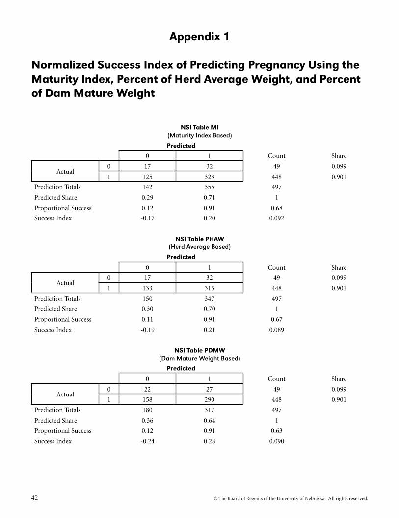
42 © The Board of Regents of the University of Nebraska. All rights reserved.
Appendix 1
Normalized Success Index of Predicting Pregnancy Using the Maturity Index, Percent of Herd Average Weight, and Percent of Dam Mature Weight
NSI Table MI(Maturity Index Based)
Predicted
0 1 Count Share
Actual0 17 32 49 0.099
1 125 323 448 0.901
Prediction Totals 142 355 497
Predicted Share 0.29 0.71 1
Proportional Success 0.12 0.91 0.68
Success Index -0.17 0.20 0.092
NSI Table PHAW(Herd Average Based)
Predicted
0 1 Count Share
Actual0 17 32 49 0.099
1 133 315 448 0.901
Prediction Totals 150 347 497
Predicted Share 0.30 0.70 1
Proportional Success 0.11 0.91 0.67
Success Index -0.19 0.21 0.089
NSI Table PDMW(Dam Mature Weight Based)
Predicted
0 1 Count Share
Actual0 22 27 49 0.099
1 158 290 448 0.901
Prediction Totals 180 317 497
Predicted Share 0.36 0.64 1
Proportional Success 0.12 0.91 0.63
Success Index -0.24 0.28 0.090

© The Board of Regents of the University of Nebraska. All rights reserved. 43
Appendix 2
Predicted Dystocia Rates/Probabilities of Dystocia Predicted by the Linear, Quadratic , and Cubic Forms of the Probit Model Using Various Maturity Index Values
Given MI Linear Quadratic Cubic
50.0 0.55 0.53 0.51
50.8 0.52 0.51 0.49
51.6 0.50 0.49 0.48
52.4 0.48 0.47 0.46
53.2 0.46 0.45 0.44
54.0 0.44 0.43 0.43
54.8 0.41 0.41 0.41
55.6 0.39 0.39 0.39
56.4 0.37 0.37 0.37
57.2 0.35 0.35 0.35
58.0 0.33 0.33 0.34
58.8 0.31 0.31 0.32
59.6 0.29 0.30 0.30
60.4 0.27 0.28 0.28
61.2 0.26 0.26 0.26
62.0 0.24 0.24 0.24
62.8 0.22 0.22 0.22
63.6 0.21 0.21 0.21
64.4 0.19 0.19 0.19
65.2 0.18 0.17 0.17
66.0 0.16 0.16 0.16
66.8 0.15 0.14 0.14
67.6 0.14 0.13 0.13
68.4 0.12 0.12 0.11
69.2 0.11 0.11 0.10
70.0 0.10 0.09 0.09
70.8 0.09 0.08 0.07
71.6 0.08 0.07 0.06
72.4 0.08 0.07 0.06
73.2 0.07 0.06 0.05

44 © The Board of Regents of the University of Nebraska. All rights reserved.
Appendix 3
Normalized Success Index of Predicting Dystocia Using Linear, Quadratic, and Cubic Forms of the Maturity Index
NSI Table For Dystocia Using The Linear MI
Predicted
0 1 Count Share
Actual0 183 145 328 0.751
1 47 62 109 0.249
Prediction Totals 230 207 437
Predicted Share 0.53 0.47 1
Proportional Success 0.80 0.30 0.56
Success Index 0.27 -0.17 0.059
NSI Table For Dystocia Using The Quadratic MI
Predicted
0 1 Count Share
Actual0 179 149 328 0.751
1 46 63 109 0.249
Prediction Totals 225 212 437
Predicted Share 0.51 0.49 1
Proportional Success 0.80 0.30 0.55
Success Index 0.28 -0.19 0.053
NSI Table For Dystocia Using The Cubic MI
Predicted
0 1 Count Share
Actual0 180 148 328 0.751
1 45 64 109 0.249
Prediction Totals 225 212 437
Predicted Share 0.51 0.49 1
Proportional Success 0.80 0.30 0.56
Success Index 0.29 -0.18 0.058

© The Board of Regents of the University of Nebraska. All rights reserved. 45
Appendix 4
Normalized Success Rate for Predicting Pregnancy Using Actual and Predicted Dystocia
NSI Table Probit Based On Actual Data With Predicted Dystocia Rates
Predicted
0 1 Count Share
Actual0 5 27 32 0.076
1 52 336 388 0.924
Prediction Totals 57 363 420
Predicted Share 0.14 0.86 1
Proportional Success 0.09 0.93 0.81
Success Index -0.05 0.06 0.046
NSI Table Probit And Pregnancy Rates Based on Predicted Dystocia Rates
Predicted
0 1 Count Share
Actual0 18 14 32 0.076
1 165 223 388 0.924
Prediction Totals 183 237 420
Predicted Share 0.44 0.56 1
Proportional Success 0.10 0.94 0.57
Success Index -0.34 0.38 0.066

46 © The Board of Regents of the University of Nebraska. All rights reserved.
Appendix 5
List of Models
AICi = ln
SSEi
T +
2Ki
T(1)
MI = 43.351 + 0.03109WtPb
– 0.1419WtBirth
+ 0.000089Age2Heifer
– 0.01272WtDam
+ 1.756AgeDam
– (<0.01) (<0.01) (<0.01) (<0.01) (<0.01) (<0.03)
0.1448Age2Dam
+ 4.888T1 + 2.645T2 + 2.588T3 (<0.03) (<0.01) (<0.01) (<0.01) (2)
MAPE =1n Σ n
i=1
| Ai – F
i |
Ai
(3)
Wt4 = 170 + 0.898Wt
3
(<0.01) (<0.01) (4)
Wt4 = 289 + 0.707Wt
5
(<0.01) (<0.01) (5)
Wt4 = 373 + 0.599Wt
8
(<0.01) (<0.01) (6)
Total Applicable Revenue (TAR) = R1 + R2 + R3 + R4 + R5 (7)
R1 = (1-PG1) × VFall
(8)
R2 = PG1 × CL × VMay
(9)
R3 = PG1 × (1 – CL) × (1 – DLCalf
) × VCalf
(10)
R4 = PG1 × (1 – CL) × (1 – DLCow
) × (1 – PG2) × VNov
(11)

© The Board of Regents of the University of Nebraska. All rights reserved. 47
R5 = PG1 × (1 – CL) × (1 – DLCow
) × PG2 × VBred
(12)
Total Applicable Cost (TAC) = C1 + C2 + C3 (13)
C1 = WtWean
× V Wean
(14)
C2 = FeedConsumed
× Cost Feed
(15)
C3 = PG1 × CDRate
× DCalving
(16)
I = c0 + b
1x
1 + b
2x
2 + ... + b
nx
n (17)
[ ] ( )∫=
∝−=
−−=≤=Iz
z
zii eIzPP 2/2
1 2
2π (18)
IPG1
= –28.372 + 0.959MI – .00756MI2
(0.03) (0.03) (0.04) (19)
ID1
= 3.559 – 0.0689 MI (<0.01) (<0.01) (20)
ID2
= 1.504 – 0.000575 MI2
(<0.01) (<0.01) (21)
ID3
= .816 – 0.00000636 MI3
(<0.04) (0.01) (22)
IPG2
= 1.645 – 0.637 D (<0.01) (<0.01) (23)
ˆIPG2
= 1.8531 – 0.0165 Dc
(<0.01) (<0.01) (24)

48 © The Board of Regents of the University of Nebraska. All rights reserved.
WtFall
= 388.8 – 2.47 × 10⁻⁵ Wt3Birth
+ 2.05 × 10⁻⁷ Wt3Wean
+ 1.98×10⁻³ Wt2Pb
– 1.48 × 10⁻⁶ Wt3Pb
– 23.26T1 – 16.33T2 – 27.17T3 (<0.01) (0.03) (0.02) (<0.01) (<0.01) (<0.01) (<0.01) (<0.01) (25)
VFall
= 253.56 + 0.67WtFall
+ 5.51Yr2001
– 89.13Yr2002
+ 67.44Yr2003
+ 174.67Yr2004
+ 118.87Yr2005
+ 108.83Yr2006
+ 93.50Yr2007
(<0.01) (<0.01) (0.20) (<0.01) (<0.01) (<0.01) (<0.01) (<0.01) (<0.01) (26)
WtMay
= –371.73 + 0.0453WtDam
+ 0.687WtBirth
+ 0.000325Wt2Pb
+ 1.879WtPG1
– 0.000785Wt2PG1
(0.05) (<0.01) (<0.01) (<0.01) (<0.01) (<0.01)
– 28.646T1 – 13.231T2 – 9.987T3 (<0.01) (<0.01) (0.01) (27)
Wt May
= Wt
Fall + Wt
PG2
2 (28)
VCalf
= 259.29 + 0.751WtCalf
– 57.466Hfr – 40.652Yr2001
– 71.298Yr2002
+ 28.226Yr2003
– 79.055Yr2004
+ 108.93Yr2005
+ (<0.01) (<0.01) (<0.01) (<0.01) (<0.01) (<0.01) (<0.01) (<0.01)
5.591Yr2006
– 11.702Yr2007
(0.04) (<0.01) (29)
WtCalf
= –463.66 + 23.904Str + 2.264CalfAge
– 0.439WtBirth
+ 1.381WtPb
– 0.000852Wt2Pb
– 32.988T1 – 20.811T2 – (<0.01) (<0.01) (<0.01) (<0.044) (<0.01) (0.02) (<0.01) (<0.01)
16.036T3 – 17.229 BreedSireChange (<0.01) (<0.01) (30)
CalfAge
= 147.1+9.958 MI – .076193 MI2
(0.25) (0.025) (0.017) (31)
WtNov
= –743.46+0.0906WtDam
+ 1.373WtBirth
+ 0.000650Wt2Pb
+ 2.759WtPG1
– 0.00157Wt2PG1
– 57.291T1 – (0.05) (<0.01) (<0.01) (<0.01) (<0.01) (<0.01) (<0.01)
26.461T2 – 19.973T3 (<0.01) (<0.01) (32)

© The Board of Regents of the University of Nebraska. All rights reserved. 49
VBred (ij)
= 394.49 – 518.25 AgedGroup(i)
– 357.11 MAgedGroup(i)
+ .68546 AvgWtGroup (i)
(<0.01) (<0.01) (<0.01) (<0.01) (33)
VBred(ij)
= 417.05 – 507.47 AgedGroup(i)
– 344.18 MAgedGroup(i)
+ .64761 AvgWtGroup(i)
+ 29.70 Year
ij
(<0.01) (<0.01) (<0.01) (<0.01) (0.23) (34)
WtWean
= 235.23 + 1.44WtBirth
+ 1.07 × 10⁻⁵ Age3Wean
+ 1.30 Age2Dam
– 0.0993 Age3Dam
(<0.01) (<0.01) (<0.01) (<0.01) (<0.01) (35)
MPF = TAR – TAC (36)
MPF = (R1 + R2 + R3 + R4 + R5) – (C1 + C2 + C3) (37)
MPF = [((1-PG1) × VFall
) + (PG1 × CL × VMay
) + (PG1 × (1 – CL) × (1 – DLCalf
) × VCalf
) + (PG1 × (1 – CL) × (1 – DLCow
) ×
(1 – PG2) × VNov
) + (PG1 × (1 – CL) × (1 – DLCow
) × PG2 · VBred
)] – [(WtWean
× V Wean
) + (FeedConsumed
× Cost Feed
) +
(PG1 × CDRate
× DCalving
) (38)
WtBirth
= 57.895+0.0211WtDam
(<0.01) (<0.01) (39)
WtWean
= 235.23 + 1.44WtBirth
+ 1.07 × 10⁻⁵ Age3Wean
+ 1.30 Age2Dam
– 0.0993 Age3Dam
(<0.01) (<0.01) (<0.01) (<0.01) (0.03) (40)
WtPre-Breed
= 110.86+0.622WtBirth
+ 0.900WtWean
+ 107.46T1 + 54.56T2 + 64.11T3 (<0.01) (<0.01) (<0.01) (<0.01) (<0.01) (<0.01) (41)
MPFi = –3975.90 + 153.89 MI
i – 1.24MI2
i
(<0.01) (<0.01) (<0.01) (42)
TAR
i = –3356.30 + 152.74 MI
i – 1.20 MI2
i
(<0.01) (<0.01) (<0.01) (43)
TACi = 619.61–1.20 MI
i + .039 MI2
i
(<0.01) (0.12) (<0.01) (44)

50 © The Board of Regents of the University of Nebraska. All rights reserved.
Appendix 6
2003, 2004, and 2005 Modified Profit Function Results
Ration # YearCow Line
ID #Dam
WeightDamAge
BirthWt
Pre-Breeding Age (Days)
Weaning Weight
Pre-Breeding Weight MI Score
Highest Ranked Heifers Using the MPF
1 2003 5280 1420 5 87.9 426 488.7 711.8 61.2
1 2004 4992 1420 5 87.9 424 485.8 709.2 60.9
1 2005 5280 1420 5 87.9 426 488.7 711.8 61.2
2 2003 9312 1420 5 87.9 454 536.1 701.5 60.8
2 2004 9312 1420 5 87.9 454 536.1 701.5 60.8
2 2005 9600 1420 5 87.9 456 539.9 704.9 61.1
3 2003 9600 1420 5 87.9 456 539.9 714.5 61.3
3 2004 9312 1420 5 87.9 454 536.1 711.0 61.0
3 2005 9600 1420 5 87.9 456 539.9 714.5 61.3
4 2003 9621 1200 6 83.2 456 538.6 646.2 60.2
4 2004 9620 1180 6 82.8 456 537.9 645.4 60.5
4 2005 9619 1160 6 82.4 456 537.3 644.6 60.8
Ration # Year Cow Line ID #
Dam Weight
Dam Age
Birth Wt
Pre-Breeding Age (Days)
Weaning Weight
Pre-Breeding Weight
MI Score
Lowest Ranked Heifers Using the MPF
1 2003 9633 800 7 74.8 456 530.8 741.4 74.2
1 2004 9633 800 7 74.8 456 530.8 741.4 74.2
1 2005 9633 800 7 74.8 456 530.8 741.4 74.2
2 2003 288 1420 11 87.9 390 449.1 623.4 50.2
2 2004 288 1420 11 87.9 390 449.1 623.4 50.2
2 2005 288 1420 11 87.9 390 449.1 623.4 50.2
3 2003 288 1420 11 87.9 390 449.1 632.9 50.4
3 2004 288 1420 11 87.9 390 449.1 632.9 50.4
3 2005 288 1420 11 87.9 390 449.1 632.9 50.4
4 2003 288 1420 11 87.9 390 449.1 568.8 45.9
4 2004 288 1420 11 87.9 390 449.1 568.8 45.9
4 2005 288 1420 11 87.9 390 449.1 568.8 45.9