JOURNAL OF AIRCRAFTVol. 33, No. 1, January-February 1996

Helicopter Rotor Blade Computation in Unsteady FlowsUsing Moving Overset Grids

Jasim Ahmad*Sterling Software, Moffett Field, California 94035-1000

andEarl P. N. Duquet

U.S. Army Aeroflightdynamics Directorate, Moffett Field, California 94035-1000

An overset grid thin-layer Navier-Stokes code has been extended to include dynamic motion of helicopterrotor blades through relative grid motion. The unsteady flowfield and airloads on an AH-IG rotor in forwardflight were computed to verify the methodology and to demonstrate the method's potential usefulness towardscomprehensive helicopter codes. In addition, the method uses the blade's first harmonics measured in the flighttest to prescribe the blade motion. The solution was impulsively started and became periodic in less than threerotor revolutions. Detailed unsteady numerical flow visualization techniques were applied to the entire unsteadydata set of five rotor revolutions and exhibited flowfield features such as blade vortex interaction and wake roll-up. The unsteady blade loads and surface pressures compare well against those from flight measurements.Details of the method, a discussion of the resulting predicted flowfield, and requirements for future work arepresented. Overall, given the proper blade dynamics, this method can compute the unsteady flowfield of ageneral helicopter rotor in forward flight.

Introduction

T HE accurate computation of a helicopter flowfield is es-sential for proper and efficient airload predictions in for-

ward flight and hover. The constantly changing aerodynamicenvironment and loads are important features of rotorcraftaerodynamics. Strong tip vortices in the rotor wakes dominatethe flowfield to produce a highly unsteady and nonuniforminduced velocity field at the rotor disk. Recent emphasis onnumerical simulation procedures for complex flows have madeit possible to accurately obtain rotor blade aerodynamic char-acteristics by solving the governing differential equations.

Descriptions of various computational fluid dynamics (CFD)methods for rotorcraft problems based on the solution of full-potential, Euler, and Navier-Stokes equations can be foundin the literature. Notable among them is the introduction ofembedded or overset grid scheme to the existing single gridscheme by Duque and Srinivasan.1 Also, Srinivasan et al.2-3

used a thin-layer Navier-Stokes method for forward-flightsimulation of a nonlifting rotor blade as well as rotor in hover.Chen et al.4 and Agarwal and Deese5 solved the Euler equa-tions.

Unlike fixed wing aircraft, the helicopter airloads dependgreatly upon the unsteady dynamic motion of the blades. Tomodel the blade motion, comprehensive helicopter analysismethods have been developed that use aerodynamic and wakemodels coupled to structural dynamic models. The aerody-namics are typically based upon lifting-line theory and dependupon either linear methods or two-dimensional experimentalairfoil data with corrections for unsteady and three-dimen-sional effects.

Presented as Paper 94-1922 at the AIAA 12th Applied Aerody-namics Conference, Colorado Springs, CO, June 20-22, 1994; re-ceived Sept. 23, 1994; revision received May 10, 1995; accepted forpublication June 24, 1995. This paper is declared a work of the U.S.Government and is not subject to copyright protection in the UnitedStates.

* Research Scientist, NASA Ames Research Center, MS 258-1.Member AIAA.

tResearch Scientist, NASA Ames Research Center, Aviation andTroop Command. Member AIAA.

Notable among the comprehensive helicopter analysis codesis CAMRAD/JA by Johnson.6 To account for compressibility,three-dimensional effects, and arbitrary blade geometries,Strawn and Tung7 coupled CAMRAD to the full potentialrotor (FPR) code. Strawn et al.8 demonstrated the capabilityto model rotors in forward flight using the coupled CAMRADand FPR by computing the airloads of the Puma rotor.

Hernandez and Johnson9 used the coupled CAMRAD/JA-FPR method to compute the AH-IG rotor in forward flight.They were able to compare well against flight test data. Inaddition, they found that tip core size specifications have alarge effect upon the predicted rotor loads.

Ramachandran et al.10 developed a method based upon thevorticity-embedding technique. This method solves the un-steady full potential equation on a Eulerian grid with an over-set Lagrangian vortical velocity field. He also applied his methodto the forward flight of the AH-IG rotor system with favorablecomparisons to flight tests.

All of the above methods use single-structured grids. Singlegrids have limited use. For example, it would be very difficultto use a single-structured grid to investigate the aerodynamicinterference between either a rotor and fuselage or the aero-dynamic interference between a rotor and the rotor hub. Inaddition, almost all of the above methods use wake modelsto include the influence of the wake. Wake models limit themethod's generality and require considerable adjustments totheir approximations to obtain accurate solutions.

The work summarized herein uses an alternative gridingmethod known as overset grids or the Chimera method11 toallow for blade motions and to accurately compute the vorticalwake from first principles. The overset-grid scheme greatlysimplifies arbitrary blade motions, which is important inachieving trimmed flight conditions, as well as in predictingairloads accurately in an effort to develop a comprehensivehelicopter analysis method. Also, with overset grids one canmore easily discretize the domain with simple well-definedgrids that accurately compute the rotor wake.

Until recently, few methods were able to solve the transientflow about multiple bodies moving relative to one another.Meakin12 computed the unsteady flowfield of the V-22 tiltro-tor aircraft, including the rotor rotation, by solving the un-

54

Dow

nloa

ded

by R

OK

ET

SAN

MIS

SLE

S IN

C. o

n N

ovem

ber

2, 2

014

| http

://ar

c.ai

aa.o

rg |

DO

I: 1

0.25

14/3

.469

02

AHMAD AND DUQUE 55

steady thin-layer Navier-Stokes equations on moving oversetgrids. To accomplish this calculation, he developed a methodthat determines the interpolation coefficients between theoverset grids. His domain connectivity algorithm (DCF) wasverified in detail in his work. But the set of flight conditionshe considered were hypothetical and did not include the dy-namic pitch, flap, or lag motions of the rotor blades. Themethod presented here accounts for the blade motion by ap-propriately moving the overset grid system according to theblade harmonics measured in a flight test.

In summary, a numerical method that computes the un-steady flowfield of a helicopter rotor in forward-flight or hoveris presented. The method solves the thin-layer Navier-Stokesequations on a system of moving overset grids and uses theblade harmonics measured in flight to prescribe the blademotions. Comparisons between computed and flight-test un-steady blade loads and surface pressures of the AH-1G heli-copter are presented. Numerical flow visualizations exhibitflowfield features such as blade-vortex interaction and wakeroll-up. This article provides details of the method, a discus-sion of the resulting predicted flowfield, and demonstratesthe capability to model the unsteady flowfield of an arbitraryhelicopter rotor in forward flight.

MethodologyAlgorithm

The single-grid flow solver developed by Srinivasan et al.2with overset-grid modifications implemented by Duque andSrinivasan1 was employed in the study. Calculations by Sri-nivasan and Ahmad13 have demonstrated the method's ver-satility by computing the hovering flowfield of a rotor andwhirl stand. The method solves the thin-layer Navier-Stokesequations shown in Eq. (1):

(1)

where Q = J~l(p,p^,pv,po), e) is the vector of the conservedvariables, density, momentum^ and ^energy^ scaled by thetransformation Jacobian, and E, F, G, and S are the scaledinviscid and viscous flux vectors.

With overset grids a sequence of grids are placed such thatthey lie arbitrarily within a primary grid. For example, Fig.1 provides an example where an airfoil curvilinear grid lieswithin a background Cartesian grid. The airfoil grid capturesfeatures such as the boundary layers, tip vortices, and shocks,etc. The background grid surrounds the airfoil grid and carriesthe solution to the far field. The background grid was gen-erated with some knowledge of the airfoil's surface and outerboundary locations. Consequently, some of the backgroundgrid points lie within the airfoil's solid body regions and mustbe removed from the solution. Once removed, hole regionsremain within the interior of the larger background grid andcreate a set of boundary points known as hole-fringe points.The airfoil grid interpolates data to the background grid atthe background's hole-fringe points. Conversely, the back-ground grid interpolates data to the airfoil grid at the airfoilouter boundary points.

Within each separate overset grid, different flow solvermethods may be used to solve the governing equations ofmotion. The current method uses an implicit upwind methodfor all of the individual grids. The method advances the so-lution in time using the lower-upper symmetric Gauss-Siedel(LU-SGS) implicit scheme by Yoon and Jameson14 shownin Eqs. (2). The scheme is third-order accurate in space andfirst-order accurate in time:

Background Grid

G* = -- -7BAf&-^S> <2** = Z)Q*

AQ = U~1Q*

Airfoil Grid

Hole Fringe Points

Airfoil Outer Boundary Points

Fig. 1 Schematic of overset grid system.

The matrices L and U are formed by performing eitherbackward or forward differences on the appropriate flux Ja-cobians A, B, or C as shown in Eqs. (3). In Eqs. (3), Af isthe time step, A^ and V^ represent forward and backwarddifferences, respectively, / is the identity matrix, and or is thespectral radius. The matrix D is a diagonal matrix that com-pletes the back-solve process. This decomposition scheme re-duces the required floating point operations in comparison toblock tridiagonal methods:

D = / + - + C~ 4-(3)

where A± = A ± ax.With overset grids, the additional array IB marks the hole

regions within the grid interior by taking on the value of 0.Outside of the hole and in the valid regions of the flowfieldthe IB array equals 1. The IB array removes the hole regionsfrom the solution set as shown in Eqs. (2).

The flux terms use a Roe upwind-biased scheme for allthree coordinate directions with higher-order MUSCL-typelimiting to model the shocks accurately.15 The resulting fluxdifferences are shown in Eq. (4):

(4)

At the hole fringe points the flux evaluations reduce tosecond order at the resulting interior boundaries by modifyingthe primitive variable evaluations with the IB array. Equation(5) shows the ^-coordinate flux evaluations:

E(QL, QK) E(QL) - \A(QL, QR)\(QK -(5)

The primitive variable quantities Q are obtained by first-order extrapolation functions at boundaries or third orderaway from boundaries. As shown in Eqs. (6), these quantitiesdrop to first order through the use of the IB array:

QL = [KG, -- Gy)

(6)

(2)

Finally, the flow solver assumes fully turbulent flow for theblades and inviscid flow in background grids. The simple al-gebraic turbulence model of Baldwin and Lomax16 is used toestimate the eddy viscosity.

Dow

nloa

ded

by R

OK

ET

SAN

MIS

SLE

S IN

C. o

n N

ovem

ber

2, 2

014

| http

://ar

c.ai

aa.o

rg |

DO

I: 1

0.25

14/3

.469

02

56 AHMAD AND DUQUE

Fig. 2 Moving overset grid schematic.

In overset grids, the quality of the solution interpolation atthe boundaries depends on the relative grid cell ARs, skew-ness, and clustering, etc. It also depends on the boundary'sproximity to high flow gradient regions. While forming thegrids, one must ensure that the boundaries have adequateoverlap, nearly equal cell ARs, and low skewness. Boundariesshould also avoid high flow gradients.

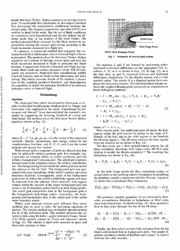
With moving overset grids, individual grids move with theirappropriate grid motion. As the grids move, the holes andhole boundaries change with time. Figure 2 provides a sche-matic for a helicopter blade in rotation, with one blade gridomitted for clarity. As the blades rotate from some time stateT0 to another time Tn, the grid attached to the blades rotatealong with them. Subsequently, the holes change with theblade rotation as shown.

To determine the grid's changing connectivity and hole points,the code known as domain connectivity functions in threedimensions (DCF3D) by Meakin12 was employed. DCF3Duses inverse mapping of the computational space to limit thesearch time and to compute hole and outer-boundary inter-polation stencils. The major expense in DCF3D is the creationof the inverse maps. However, the maps are independent ofthe relative orientation of the grids and so it repeatedly usesthe maps during the grid movement.

During the flowfield solution process, intergrid boundariesare constantly created due to the grid movement. After eachflow solution time step, grid connectivity data has to be de-termined. Currently, the flow solver (Chi-TURNS) and theconnectivity algorithm (DCF3D) are separate Fortran codes.A UNIX C-Shell script is used to join the two methods.

With each time step, DCF3D obtains the latest connectivitydata and hole points. Relevant intergrid boundary data arewritten to disk. The hole-fringe points are then checked toensure that they are introduced to the solution gradually. Theflow solver then begins the solution process by reading in theDCF3D files from disk, solving the equations of motion, andthen moving the grids to the next time step. Once complete,the solution and grids are written to disk and the whole processcontinues until the desired number of time steps have beencompleted.

Blade MotionThe method assumes rigid blade motions in flap and pitch.

The periodic blade motion for pitch and flap as a function ofblade azimuth can be described by a Fourier series10'17 asshown in Eqs. (7) and (8):

Pitch

6 = 0Q + 0U. cos ^ + 0l5 sin \fj + 62c cos '.

02, sin 2s +

Flap

ft, + j8lc cos <jS^ sin 2s + •

sin cos

(7)

(8)

Using only the mean and first blade harmonics, Eulerianangles prescribe the blade motion to the flow solver. Eulerparameters or Eulerian angles18 are useful and convenientways to express motion of rotating bodies in terms of the fixedinertial frame.

In this method, the blade rotates about its spin axis at somegiven rotational rate. At each time step, the blade rotatesthrough by an increment of ty that results in a change in pitchand flap. The incremental change in the blade position is thenimposed by transforming the position vector through succes-sive matrix multiplications as shown in Eq. (9):

T = (9)

The transformation matrix T consists of the rotation ma-trices A, B, and C. The matrices A, B, and C represent thevarious coordinate rotations. See Amirouche18 for details ofthe transformation matrices.

Grid SystemThe grid system consists of five overset grids; one for each

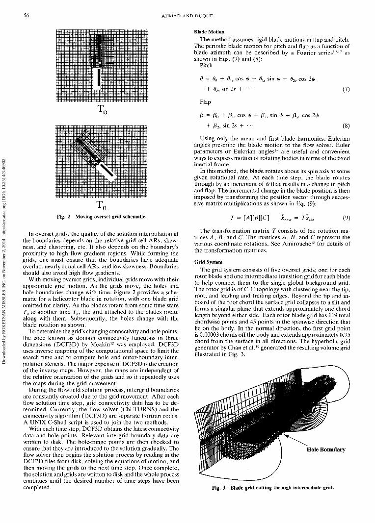
rotor blade and one intermediate transition grid for each bladeto help connect them to the single global background grid.The rotor grid is of C-H topology with clustering near the tip,root, and leading and trailing edges. Beyond the tip and in-board of the root chord the surface grid collapses to a slit andforms a singular plane that extends approximately one chordlength beyond either side. Each rotor blade grid has 119 totalchordwise points and 45 points in the span wise direction thatlie on the body. In the normal direction, the first grid pointis 0.00003 chords off the body and extends approximately 0.75chord from the surface in all directions. The hyperbolic gridgenerator by Chan et al.19 generated the resulting volume gridillustrated in Fig. 3.

Hole Boundary

Fig. 3 Blade grid cutting through intermediate grid.

Dow

nloa

ded

by R

OK

ET

SAN

MIS

SLE

S IN

C. o

n N

ovem

ber

2, 2

014

| http

://ar

c.ai

aa.o

rg |

DO

I: 1

0.25

14/3

.469

02

AHMAD AND DUQUE 57

Fig. 4 Blade grid with intergrid hole boundary.

Fig. 5 Global background grid with blade system.

To improve interpolation, each blade grid lies within anintermediate grid. The intermediate grids are Cartesian withpoints concentrated at the blade's vicinity as shown in Fig. 4.The grids extend from the hub rotation axis to approximatelyfive blade chords from the upper surface, seven chords fromthe lower, four chords in front, seven chords behind, and fivechords from the tip. Each grid contains 75 points span wise,75 points chord, and 41 points from bottom to top. Figure 4illustrates boundary planes within an intermediate grid withthe blade grid cutting through it.

The global background grid shown in Fig. 5 completes theoverset grid system. The global grid extends to four bladeradii from the hub center upstream, downstream, and to thesides. The grid also extends two blade radii above the bladeand two and one-half radii below. The grid consists of a totalof 95 x 95 x 51 points with points clustered vertically in therotor disk vicinity.

The entire moving overset system totals 1.62 million gridpoints. During the grid motions, the background grid remainsstationary as the blade and intermediate grids rotate togetherthrough it. Figure 5 highlights the relative positions of theintermediate and blade grids with respect to the backgroundgrid. The intermediate grids move only in rotation about thespin axis and subsequently create hole regions within the back-ground grid. The blade grids also rotate about the spin axis,but then also pitch and flap about those respective axes. Dur-

ing their pitch and flap motions the blade grids create holeswithin the intermediate grid as shown in Figs. 3 and 4.

Flight Test ConditionsThe flight conditions chosen as a validation case comes from

the flight tests documented by Cross and Watts20 and Crossand Tu.21 This test was chosen because of its extensive loadsurvey, acoustic measurements, and detailed blade harmonicsdata. In addition, select flight conditions have been computedby two other numerical methods.9'10 Both methods showedgood correlations with the flight test data.

The flight tests were performed with the AH-1G helicopterat NASA Ames Research Center. The rotor is a two-bladedrectangular-planform teetering rotor with the operational loadssurvey (OLS) symmetrical airfoil section, and a linear twistof -10 deg from root to tip. Each blade has an AR of 9.8.

The forward-flight case chosen is test point no. 2157 re-ported in Cross and Watts.20 This flight condition has an ad-vance ratio of 0.19, hover tip Mach number of 0.65, flightReynolds number of 9.73 x 108, and a rotor thrust coefficientequal to 0.00464. These conditions correspond to a forwardspeed of 82 kn at a rotor rotation rate of 315.9 rpm.

The first blade harmonics reported by the flight test wereused to prescribe the rotor blade motions. Table 1 lists theblade harmonics.

Results and DiscussionThe results were computed on the Numerical Aerodynamic

Simulation Facility's Cray C-90 computer located at NASAAmes Research Center. The time-accurate calculation im-pulsively starts from freestream conditions with the viscousno-slip boundary condition applied at the blade surfaces. Thetime steps for this rotor blade system correspond to approx-imately 0.3125 deg of rotation or a nondimensional time stepof 0.082. Each rotor revolution requires about 1152 time steps.The complete unsteady computation required a total of 45 hof single processor CPU time for five complete rotor revo-lutions producing approximately 40 Gbytes of flowfield data.

As noted in the previous section, the computed results usedthe first blade harmonics as measured by the flight test. How-ever, the blade collective was corrected to the value recom-mended by Ramachandran et al.,10 which allowed them tomatch the measured value of thrust. No further trim of therotor was attempted in the present investigation with the resultthat the computed thrust was about 1.8% too low. In addition,the rotor was approximately balanced in rolling (lateral) hub

Table 1 Blade first harmonics,test point 2157

0o,deg6.0

0,.v,

deg-5.5

ol(,deg1.7

Pis,deg

-0.15

Pic,deg2.13

M = 0.19, MT = 0.65, Re = 9.73 x 106, andCT = 0.00464.

—— Computation- - - • Experiment

360 720 1080 1440 1800Azimuth (degrees)

Fig. 6 Time history of normal force coefficient.

Dow

nloa

ded

by R

OK

ET

SAN

MIS

SLE

S IN

C. o

n N

ovem

ber

2, 2

014

| http

://ar

c.ai

aa.o

rg |

DO

I: 1

0.25

14/3

.469

02

58 AHMAD AND DUQUE

a) %,̂ <c..,,̂ ;, vug;'*-^. --^m

b)

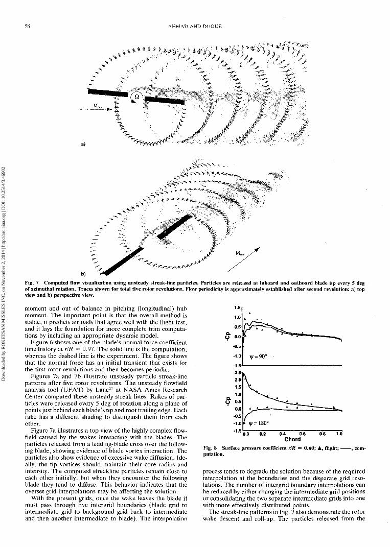
Fig. 7 Computed flow visualization using unsteady streak-line particles. Particles are released at inboard and outboard blade tip every 5 degof azimuthal rotation. Traces shown for total five rotor revolutions. Flow periodicity is approximately established after second revolution: a) topview and b) perspective view.

moment and out of balance in pitching (longitudinal) hubmoment. The important point is that the overall method isstable, it predicts airloads that agree well with the flight test,and it lays the foundation for more complete trim computa-tions by including an appropriate dynamic model.

Figure 6 shows one of the blade's normal force coefficienttime history at r/R = 0.97. The solid line is the computation,whereas the dashed line is the experiment. The figure showsthat the normal force has an initial transient that exists forthe first rotor revolutions and then becomes periodic.

Figures 7a and 7b illustrate unsteady particle streak-linepatterns after five rotor revolutions. The unsteady flowfieldanalysis tool (UFAT) by Lane22 at NASA Ames ResearchCenter computed these unsteady streak lines. Rakes of par-ticles were released every 5 deg of rotation along a plane ofpoints just behind each blade's tip and root trailing edge. Eachrake has a different shading to distinguish them from eachother.

Figure 7a illustrates a top view of the highly complex flow-field caused by the wakes interacting with the blades. Theparticles released from a leading-blade cross over the follow-ing blade, showing evidence of blade vortex interaction. Theparticles also show evidence of excessive wake diffusion. Ide-ally, the tip vortices should maintain their core radius andintensity. The computed streakline particles remain close toeach other initially, but when they encounter the followingblade they tend to diffuse. This behavior indicates that theoverset grid interpolations may be affecting the solution.

With the present grids, once the wake leaves the blade itmust pass through five intergrid boundaries (blade grid tointermediate grid to background grid back to intermediateand then another intermediate to blade). The interpolation

1.5

1.0

0.5

O 0.0

-0.5

-1.0

-1.52.52.01.51.0

5" 0.50.0

-0.5-1.0-1.5

\|/=180°

0.0 0.2 0.4 0.6Chord

0.8 1.0

Fig. 8 Surface pressure coefficient r/R = 0.60; A, flight; ——, com-putation.

process tends to degrade the solution because of the requiredinterpolation at the boundaries and the disparate grid reso-lutions. The number of intergrid boundary interpolations canbe reduced by either changing the intermediate grid positionsor consolidating the two separate intermediate grids into onewith more effectively distributed points.

The streak-line patterns in Fig. 7 also demonstrate the rotorwake descent and roll-up. The particles released from the

Dow

nloa

ded

by R

OK

ET

SAN

MIS

SLE

S IN

C. o

n N

ovem

ber

2, 2

014

| http

://ar

c.ai

aa.o

rg |

DO

I: 1

0.25

14/3

.469

02

AHMAD AND DUQUE 59

1.5!

1.0

0.5

o" 0.0-0.5

-1.0

a) -1.5

1.5

1.0

0.5

5" 0.0

-0.5

-1.0

b) -1.5

3.0!

2.0

1.0

0.0

-1.0

C) -2.0

0.9

Q.

9

3.0

2.0

1.0

0.0

-1.0

-2.0 0.0 0.2d)

0.4 0.6Chord

0.8 1.0

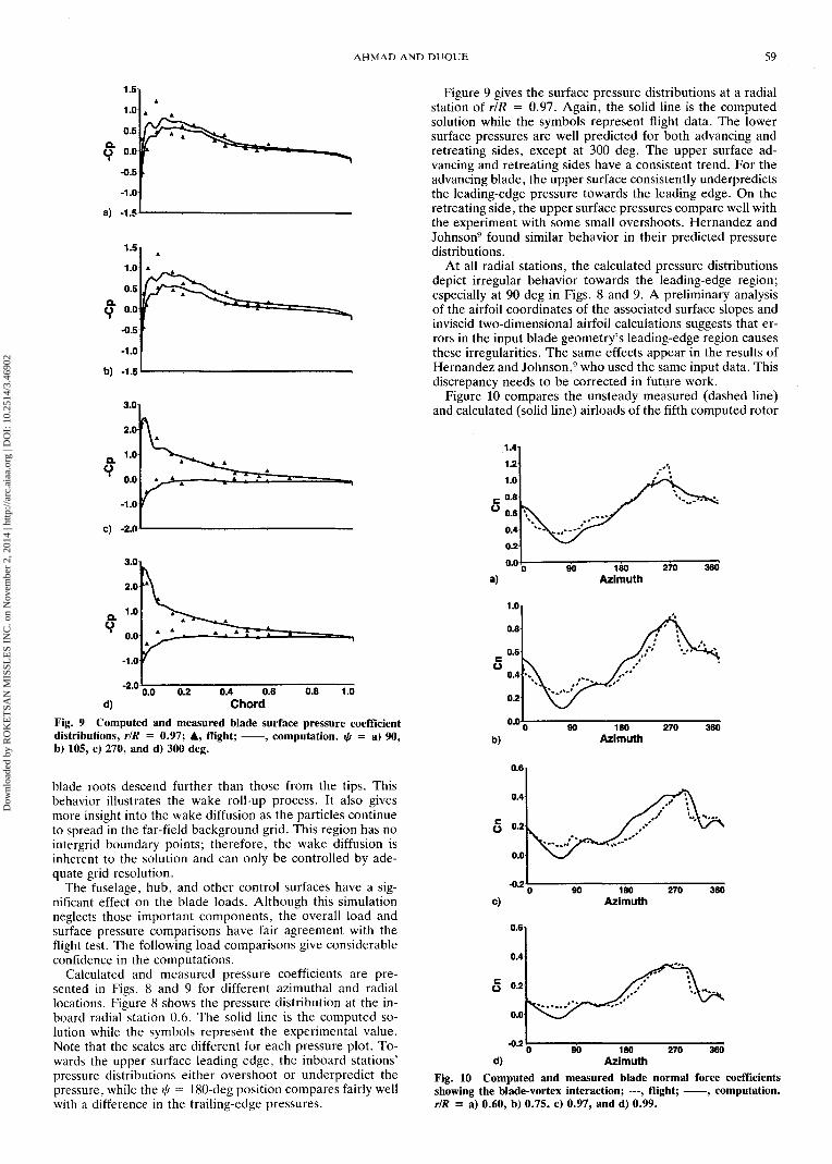
Fig. 9 Computed and measured blade surface pressure coefficientdistributions, rlR = 0.97; A, flight; ——, computation, if/ = a) 90,b) 105, c) 270, and d) 300 deg.

blade roots descend further than those from the tips. Thisbehavior illustrates the wake roll-up process. It also givesmore insight into the wake diffusion as the particles continueto spread in the far-field background grid. This region has nointergrid boundary points; therefore, the wake diffusion isinherent to the solution and can only be controlled by ade-quate grid resolution.

The fuselage, hub, and other control surfaces have a sig-nificant effect on the blade loads. Although this simulationneglects those important components, the overall load andsurface pressure comparisons have fair agreement with theflight test. The following load comparisons give considerableconfidence in the computations.

Calculated and measured pressure coefficients are pre-sented in Figs. 8 and 9 for different azimuthal and radiallocations. Figure 8 shows the pressure distribution at the in-board radial station 0.6. The solid line is the computed so-lution while the symbols represent the experimental value.Note that the scales are different for each pressure plot. To-wards the upper surface leading edge, the inboard stations'pressure distributions either overshoot or underpredict thepressure, while the i/> = 180-deg position compares fairly wellwith a difference in the trailing-edge pressures.

Figure 9 gives the surface pressure distributions at a radialstation of r/R = 0.97. Again, the solid line is the computedsolution while the symbols represent flight data. The lowersurface pressures are well predicted for both advancing andretreating sides, except at 300 deg. The upper surface ad-vancing and retreating sides have a consistent trend. For theadvancing blade, the upper surface consistently underpredictsthe leading-edge pressure towards the leading edge. On theretreating side, the upper surface pressures compare well withthe experiment with some small overshoots. Hernandez andJohnson9 found similar behavior in their predicted pressuredistributions.

At all radial stations, the calculated pressure distributionsdepict irregular behavior towards the leading-edge region;especially at 90 deg in Figs. 8 and 9. A preliminary analysisof the airfoil coordinates of the associated surface slopes andinviscid two-dimensional airfoil calculations suggests that er-rors in the input blade geometry's leading-edge region causesthese irregularities. The same effects appear in the results ofHernandez and Johnson,9 who used the same input data. Thisdiscrepancy needs to be corrected in future work.

Figure 10 compares the unsteady measured (dashed line)and calculated (solid line) airloads of the fifth computed rotor

1.4

1.2

1.0

C0.8

"0.6

0.4

0.2

0.0

a)

1.0

0.8

0.4

0.2

0.0

90 180 270 360Azimuth

b)

0.6

0.4

O 0.2

0.0

-0.2

90 180 270Azimuth

C)90 180 270 360

Azimuth

0.6

0.4

0.0

-0.2

d)90 180 270

Azimuth360

Fig. 10 Computed and measured blade normal force coefficientsshowing the blade-vortex interaction; —, flight; ——, computation.r/R = a) 0.60, b) 0.75, c) 0.97, and d) 0.99.

Dow

nloa

ded

by R

OK

ET

SAN

MIS

SLE

S IN

C. o

n N

ovem

ber

2, 2

014

| http

://ar

c.ai

aa.o

rg |

DO

I: 1

0.25

14/3

.469

02

60 AHMAD AND DUQUE

Table 2 Computed and flight test rotor forceand moment coefficients

ComputedFlight

C7,thrust

0.004550.00464

CQ,torque

0.0002270.0002196

C.»*\longitudinal-0.00022

0.0

CMy,lateral

0.0000080.0

\L = 0.19, Mr = 0.65, Re = 9.73 x 106, and a = 0.0651.

0.00?!

0.006

0.005

0.004

0.003

0.002

Integrated CT = 0.00455

180Azimuth

Fig. 11 Time history of rotor thrust.

revolution at various radial locations. The figures show strongblade vortex interaction for the advancing blade around azi-muthal locations of 70-90 deg and on the retreating sidearound 270 deg. The loads are underpredicted for the ad-vancing side. At the retreating side, loads are slightly under-predicted for the cases presented here. Blade-vortex inter-actions at outboard stations seem stronger as indicated by thenegative lift.

Table 2 lists the computed rotor force and moment coef-ficients. As shown, the rotor is not trimmed in pitch, butessentially trimmed in roll. The power is overpredicted byapproximately 15%.

Figure 11 illustrates the time variation of the integratedrotor thrust for the fifth rotor revolution. The solid line pre-sents the predicted azimuthal variation while the dashed linerepresents the time averaged or gross rotor thrust. The grossthrust agrees within 1.8% of the gross weight of the aircraftin flight.

Conclusions and Future WorkThe unsteady forward-flight flowfield of the AH-1G heli-

copter's two-bladed rotor system was computed by solvingthe thin-layer Navier-Stokes equations on moving oversetgrids. The resulting flowfield visualizations and airload com-parisons verify the method's versatility for rotorcraft prob-lems. The method efficiently obtained periodic solutions withinthree rotor revolutions. Unsteady streak lines showed thesignificant blade vortex interactions and wake roll-up. In ad-dition, the streak-line patterns showed that grid resolutionneeds improvement in the rotor wake to reduce diffusion inthe wake. Blade surface pressures compared well with theflight test data, especially at the retreating side. This com-parison was somehow surprisingly better in the inboard sec-tion. Leading-edge surface pressure irregularities point to er-rors in the original airfoil coordinate definitions. The spanwiseand integrated load data also correlates fairly well with theflight airload data and previous computations.

Although the rotor was only partially trimmed, these resultsdemonstrate the method's capabilities. To trim the rotor prop-erly, one would need to include blade dynamics by tightlycoupling the unsteady load prediction to a suitable dynamicsmodel, which is a straightforward extension to the presentformulation. This coupling would also allow for aeroelasticeffects such as torsion and bending. The inclusion of a fuselagethrough additional overset grids would further improve thesolutions.

AcknowledgmentsThe authors would like to thank K. Ramachandran for

providing the blade surface geometry and all of his subsequenthelp in this work. We would also like to thank Jeffry L. Crossfor providing valuable information regarding the flight test.Finally, the authors wish to express their appreciation to W.J. McCroskey for his help and encouragement.

References'Duque, E. P. N., and Srinivasan, G. R., "Numerical Simulation

of a Hovering Rotor Using Embedded Grids," Proceedings of the48th AHS Annual Forum and Technology Display (Washington, DC),American Helicopter Society, 1992.

2Srinivasan, G. R., Baeder, J. D., Obayashi, S., and McCroskey,W. J., "Flowfield of a Lifting Rotor in Hover: Navier-Stokes Sim-ulation," AIAA Journal, Vol. 30, No. 10, 1992, pp. 2371-2378.

'Srinivasan, G. R., and Baeder, J. D., "TURNS: A Free-WakeEuler/Navier-Stokes Numerical Method for Helicopter Rotors," AIAAJournal, Vol. 31, No. 5, 1993, pp. 959-962.

4Chen, C. L., and McCroskey, W. J., "Numerical Solutions ofForward Flight Rotor Flow Using an Upwind Method," AIAA Paper89-1846, June 1989.

sAgarwal, R. K., and Deese, J. E., "A Euler Solver for Calculatingthe Flowfield of a Helicopter Rotor in Hover and Forward Flight,"AIAA Paper 87-1427, June 1987.

Mohnson, W., CAMRAD/JA ; A Comprehensive Analytical Modelof Rotorcraft Aerodynamics and Dynamics, Vol. I, Johnson Aero-nautics, Palo Alto, CA, 1988.

7Strawn, R., and Tung, C., "The Prediction of Transonic Loadingon Advancing Helicopter Rotors," NASA TM-88238, United StatesArmy Aviation Systems Command, USAVSCOM TM 86-A-l, April1986.

<sStrawn, R., Desopper, A., Miller, J., and Jones, A., "Correlationof PUMA Airloads-Evaluation of CFD Prediction Methods," Fif-teenth European Rotorcraft Forum, Amsterdam, Sept. 1989.

l)Hernandez, F., and Johnson, W., "Correlation of Airloads on aTwo-Bladed Helicopter Rotor," International Specialist Meeting onRotorcraft Acoustics and Rotor Fluid Dynamics, PA, Oct. 1991.

"'Ramachandran, K., Schlechtriem, S., Caradonna, F. X., andSteinhoff, J. S., "Free-Wake Computation of Helicopter Rotor Flow-field in Forward Flight," AIAA Paper 93-3079, July 1993.

"Steger, J. L., Dougherty, F. C., and Benek, J. A., "A ChimeraGrid Scheme," Advances in Grid Generation, edited by K. N. Ghiaand U. Chia, American Society of Mechanical Engineers FED-5,1983, pp. 59-69.

12Meakin, R., "Moving Body Overset Grid Methods for CompleteAircraft Tiltrotor Simulations," AIAA Paper 93-3350, July 1993.

"Srinivasan, G. R., and Ahmad, J. U., "Navier-Stokes Simulationof Rotor-Body Flowfield in Hover Using Overset Grids," NineteenthEuropean Forum, Cernobbio, (Como) Italy, 1993.

l4Yoon, S., and Jameson, A., "An LU-SSOR Scheme for the Eulerand Navier-Stokes Equations," AIAA Paper 87-0600, Jan. 1987.

"Van Leer, B., Thomas, J. L., Roe, P. L., and Newsome, R. W.,"A Comparison of Numerical Flux Formulas for the Euler and Na-vier-Stokes Equations," AIAA Paper 87-1104, June 1987.

l6Baldwin, B. S., and Lomax, H., "Thin-Layer Approximation andAlgebraic Model for Separated Turbulent Flow," AIAA Paper 78-0257, Jan. 1978.

l7Johnson, W., Helicopter Theory, Princeton Univ. Press, Prince-ton, NJ, 1980.

lsAmirouche, F. M. L., Computational Methods in Multibody Dy-namics, Prentice-Hall, Englewood Cliffs, NJ, 1992.

|l)Chan, W. M., Chiu, I. T., and Buning, P. G., "User's Manualfor the Hyperbolic Grid Generator and the HGUI Graphical UserInterface," NASA TM 108791, Oct. 1993.

20Cross, J. F., and Watts, M. E., "Tip Aerodynamics and AcousticsTest," NASA Ref. Pub. 1179, Dec. 1988.

2lCross, J. F., and Tu, W., "Tabulation of Data from the TipAerodynamics and Acoustics Test," NASA TM 102280, Nov. 1990.

22Lane, D. A., "UFAT—A Particle Tracer for Time-DependentFlow Fields," Proceedings of IEEE Visualization '94 (Washington,DC), 1994, pp. 257-264.

Dow

nloa

ded

by R

OK

ET

SAN

MIS

SLE

S IN

C. o

n N

ovem

ber

2, 2

014

| http

://ar

c.ai

aa.o

rg |

DO

I: 1

0.25

14/3

.469

02