Embed Size (px)
Citation preview

Helsinki University of Technology Laboratory of Biomedical Engineering
Department of Engineering Physics and Mathematics
Teknillinen korkeakoulu Laaketieteellisen tekniikan laboratorio
Teknillisen fysiikan ja matematiikan osasto
Espoo 2002
CONTEXTUAL DETECTION OF
FMRI ACTIVATIONS AND MULTIMODAL
ASPECTS OF BRAIN IMAGING
Eero Salli
Dissertation for the degree of Doctor of Science in Technology to be presented with due permis-sion of the Department of Engineering Physics and Mathematics for public examination anddebate in Auditorium F1 at Helsinki University of Technology (Espoo, Finland) on the 8th ofAugust, 2002, at 12 noon.

ISBN (printed) 951-22-6029-8ISBN (pdf) 951-22-6030-1
Picaset OyHelsinki 2002
Abstract
Functional magnetic resonance imaging (fMRI) is a non-invasive method which can be usedto indirectly localize neuronal activations in the human brain. Functional MRI is based onchanges in the blood oxygenation level near the activated tissue. In an fMRI experiment,a stimulus is given to a subject or the subject is asked to conduct a physical or cognitivetask. During the experiment, a nuclear magnetic resonance signal is measured outside thehead, and time series of three-dimensional image volumes are constructed. The object of thisthesis is to study the localization of activation regions from the constructed time series aswell as multimodal aspects of brain imaging. The localization of activation regions typicallyconsists of the following phases: preprocessing of the four-dimensional spatiotemporal data,computation of a statistic image, and detection of statistically significantly activated regionsfrom the statistic image. The statistic image is a three-dimensional map, which shows thestatistical significance of the measured experimental effect at voxel level. The detection andlocalization of the activated regions can be carried out by segmenting the statistic image intoactivated and non-activated regions. The segmentation is difficult because the statistic imagesare often noisy and high specificity requirements are set for the activation localization. In thisthesis, a computationally efficient segmentation method has been developed. The method isbased on the utilization of contextual information from the 3-D neighborhood of each voxelby using a Markov random field model. The method does not require assumptions aboutthe intensity distribution of the activated voxels. The method has been tested using bothsimulated and measured fMRI data. The use of contextual information increased the detectionrate of weakly activated regions. In the simulation experiments, spatial autocorrelations in thenoise term altered overall false-positive rates only little. It was also demonstrated that thedeveloped method preserved spatial resolution better than the commonly used linear spatialfiltering. In repeated fMRI experiments, variation in the activated regions obtained by thedeveloped method was about the same as or less than with other widely used methods. Inaddition to the activation localization, the use of multimodal data, including the comparisonof fMRI and magnetoencephalographic (MEG) data, is discussed in this thesis. This thesisalso includes multimodal visualization examples created from MEG, single photon emissioncomputed tomography, fMRI and structural magnetic resonance imaging data.
Keywords: fMRI, activation localization, segmentation, contextual information, multimodal-ity, visualization
i
Contents
List of publications ii
List of abbreviations and symbols iii
1 Introduction 1
2 Medical imaging modalities 4
2.1 Magnetic resonance imaging . . . . . . . . . . . . . . . . . . . . . . . . . . . . . 4
2.2 Functional magnetic resonance imaging . . . . . . . . . . . . . . . . . . . . . . . 4
2.3 Other functional imaging or measurement techniques . . . . . . . . . . . . . . . 7
3 Segmentation methods related to this work 9
3.1 Markov random field-based segmentation . . . . . . . . . . . . . . . . . . . . . . 9
3.2 Goals of segmentation . . . . . . . . . . . . . . . . . . . . . . . . . . . . . . . . 11
3.3 Minimization of energy function . . . . . . . . . . . . . . . . . . . . . . . . . . . 12
3.4 Approach used in this thesis . . . . . . . . . . . . . . . . . . . . . . . . . . . . . 15
Box: Contextual clustering algorithm . . . . . . . . . . . . . . . . . . . . . . 16
4 Data analysis 18
4.1 Acquisition of data and goals of fMRI data analysis . . . . . . . . . . . . . . . . 18
4.2 Preprocessing of fMRI data . . . . . . . . . . . . . . . . . . . . . . . . . . . . . 19
4.3 Computation of statistic images . . . . . . . . . . . . . . . . . . . . . . . . . . . 21
4.4 Detection of activations from statistic images . . . . . . . . . . . . . . . . . . . . 23
4.5 Approach used in this thesis . . . . . . . . . . . . . . . . . . . . . . . . . . . . . 28
4.6 Testing or modelling activations? . . . . . . . . . . . . . . . . . . . . . . . . . . 35
5 Multimodal imaging 36
5.1 Registration . . . . . . . . . . . . . . . . . . . . . . . . . . . . . . . . . . . . . . 36
5.2 Comparing and combining fMRI and MEG . . . . . . . . . . . . . . . . . . . . . 36
5.3 Segmentation and multimodal visualization . . . . . . . . . . . . . . . . . . . . . 38
6 Concluding remarks 41
7 Summary of publications 42
References 45
ii
List of publications
This thesis consists of an overview and of the following six publications:
I E. Salli, H. J. Aronen, S. Savolainen, A. Korvenoja and A. Visa (2001). Contextual
clustering for analysis of functional MRI data. IEEE Trans. Med. Imaging 20:403–414.
II E. Salli, A. Visa, H. J. Aronen, A. Korvenoja and T. Katila (1999). Statistical segmenta-
tion of fMRI activations using contextual clustering. In Proc. of the 2nd International con-
ference on Medical Image Computing and Computer Assisted Intervention (MICCAI’99).
C. Taylor, A. Colchester (Eds.). Springer. Lect. Notes Comput. Sci. 1679:481–488.
III E. Salli, A. Korvenoja, A. Visa, T. Katila and H. J. Aronen (2001). Reproducibility of
fMRI: Effect of the use of contextual information. NeuroImage 13:459–471.
IV A. Korvenoja, J. Huttunen, E. Salli, H. Pohjonen, S. Martinkauppi, J. M. Palva, L. Lauro-
nen, J. Virtanen, R. J. Ilmoniemi and H. J. Aronen (1999). Activation of multiple cortical
areas in response to somatosensory stimulation: Combined magnetoencephalographic and
functional magnetic resonance imaging. Hum. Brain Mapp. 8:13–27.
V H. Pohjonen, O. Sipila, V.-P. Poutanen, S. Bondestam, K. Somer, E. Salli, A. Korvenoja,
P. Nikkinen, H. J. Aronen, R. J. Ilmoniemi, T. Katila, K. Liewendahl and C.-G. Standert-
skjold-Nordenstam (1996). Hospital-wide PACS: multimodal image analysis using ATM
network. In Computer Assisted Radiology: Proc. of the International Symposium on Com-
puter and Communication Systems for Image Guided Diagnosis and Therapy (CAR’96).
H. U. Lemke, M. W. Vannier, K. Inamura, A. G. Farman (Eds.). Elsevier. Pages 399–404.
VI H. Pohjonen, P. Nikkinen, O. Sipila, J. Launes, E. Salli, O. Salonen, P. Karp, J. Yla-
Jaaski, T. Katila and K. Liewendahl (1996). Registration and display of brain SPECT
and MRI using external markers. Neuroradiology 38:108–114.
iii
List of abbreviations and symbols
BOLD blood oxygenation level-dependentCNR contrast-to-noise ratioCSF cerebral spinal fluidECD equivalent current dipoleEPI echo-planar imagingFIR finite impulse responsefMRI functional magnetic resonance imagingFPQ fundamental power quotientFPR false-positive rateFWHM full width at half maximumGLM general linear modelGM gray matterHRF hemodynamic response functionICM iterated conditional modesKS Kolmogorov-SmirnovMAP maximum a posterioriMEG magnetoencephalographyML maximum likelihoodMMP maximum marginal probabilityMR magnetic resonanceMRF Markov random fieldMRI magnetic resonance imagingN(µ, σ2) Normal distribution with mean µ and variance σ2
NIR Near-infraredPET positron emission tomographyRF radio frequencyROC receiver operator characteristicSA simulated annealingSI statistic imageSMA supplementary motor areaSMI primary sensorimotor cortexSNR signal-to-noise ratioSPE(C)T single photon emission (computed) tomographySPM statistical parametric mappingSVD singular value decompositionWM white mattern-D n-dimensional

1
1 Introduction
Our understanding of the human brain and its function at macroscopic, microscopic and molec-
ular levels has greatly increased during the last decades. Remarkable advances have been made
in molecular and cellular level research and in gene technology including the identification
of genes responsible for various diseases and results of single-neuron recordings (Kandel and
Squire, 2000). The development of functional brain imaging methods producing time series of
volumetric data, like positron emission tomography (PET) and functional magnetic resonance
imaging (fMRI), has provided an ability to monitor neural activity in the whole brain area.
The functional imaging methods produce huge amount of data, which has created a need for
efficient data analysis, processing and visualization methods.
Magnetic resonance imaging (MRI) is nowadays the ultimate method in obtaining images
of human brain structure non-invasively. At the beginning of the 90s it was noted that the
principles of MRI can also be used to image the function of the brain (Ogawa et al., 1990,
1992; Belliveau et al., 1991; Kwong et al., 1992). In most fMRI experiments, blood serves
as an endogenous contrast agent to image hemodynamics accompanying neuronal activation.
It is said that fMRI has revolutionized cognitive neuroscience and neurofunctional imaging
(Menon, 2001; Lai et al., 2000). Functional MRI, together with other brain mapping methods
like PET, electroencephalography (EEG) and magnetoencephalography (MEG), has increased
knowledge of the human brain function. For example, new information has been obtained
about motor function, perception, face recognition, learning and memory (Rosen et al., 1998;
Rowe and Frackowiak, 1999; Moonen and Bandettini, 2000). As a non-invasive method fMRI
can also be used on children and the studies can be repeated several times on a same subject.
This allows the monitoring of changes in cortical organization during learning and development.
Potential clinical applications of fMRI include pre-surgical localization of functionally important
brain areas, detection of functional abnormalities in developmental disorders, monitoring of
brain damage and recovery of function, monitoring of effectiveness of therapeutic interventions
(e.g. drugs and different rehabilitation strategies) and investigation of cerebral correlates of
mental illness (Moonen and Bandettini, 2000; Turner and Ordidge, 2000).
While fMRI measures the relatively slow hemodynamic changes associated with neural ac-
tivity, EEG and MEG measure the electric or magnetic fields generated by neuronal activity.
The temporal and spatial characteristics of the methods complement each other. Single photon
emission computed tomography (SPECT) provides information about physiological function
and can be used to diagnose various abnormalities like cerebral infarcts, brain tumors, in-
flammatory diseases and epilepsy, among many other applications. Anatomical localization of
the abnormalities is sometimes difficult but can be improved by adding structural information
from MR images. These examples illustrate that different imaging modalities provide comple-
mentary information, and fusing the data from different imaging modalities is often beneficial.
Some related multimodal aspects, like comparison of different modalities and visualization, are
presented in this work.
A frequent goal of fMRI data analysis is to recognize activated brain areas, i.e. image
regions whose intensity changes are induced by the stimulus given to a subject. The analysis
of fMRI data is complicated for several reasons. Task- or stimulus-induced signal-change-to-
signal-noise ratio (contrast-to-noise ratio, CNR) is often low. Noise sources include thermal
2 1 INTRODUCTION
noise, physiological fluctuations, effects caused by movements of the subject and instrumental
instabilities. In many cases (e.g. with visual stimulus), the voxels1 of the strongest “activations”
may show signal changes of tens of percents, especially when small voxels are used to reduce
partial volume effects [e.g. Oja et al. (1999a)]. However, the histogram of activation-related
signal changes may be broad and include small changes. Large signal changes often arise
from relatively large venous vessels (Kim et al., 2000) rather than from the smaller venules
and capillaries closer to the activated neuronal tissue. Typical magnitudes of signal changes in
tasks involving primary sensory or primary motor areas are of the order of a few percent, and in
cognitive tasks of the order of one percent or so. To detect these subtle changes from the noise,
the measurements are usually repeated several times over a long period of time, which, in turn,
may lead to problems associated with subject motion and scanner instabilities. The second
complication of fMRI data analysis is the large size of datasets, typically tens of megabytes
in size. Analysis of these data sets requires a great deal of storage space, powerful computers
and efficient data analysis methods. In addition, autocorrelated noise makes it more difficult
to draw statistical inferences.
In this work, the localization of the activated regions has been studied as a segmentation
problem: how to divide an image into activated and non-activated areas. The term “segmenta-
tion” implicitly includes not only the detection and localization, but also the delineation of the
activated regions. Usually a 3-D statistic image (SI), also called a statistical map, is computed
from the four-dimensional spatiotemporal fMRI data after preprocessing steps. The effects of
signal variations originating from physiology or scanner instabilities are minimized by means
of study design and data preprocessing and during the computation of the SI. The intensities
of non-activated voxels of the SI are assumed to follow a known distribution, e.g. the standard
normal distribution N(0, 1), and activated voxels unknown distributions. The segmentation
of the SI represents a special type of segmentation problem in which the distribution of the
background (null distribution) voxels is known but the distributions of the object (activated
regions) voxels are not. A traditional approach is to threshold the computed SI. Together the
computation of the SI and its thresholding consist of a large number of hypothesis tests, one
for each voxel. A voxel is considered to be activated if the test rejects a null hypothesis that
the voxel is not activated. It is important to note that in addition to the task-induced signal
change, the intensities of the activated voxels in the SI depend on the noise level and on the
number of data points in the measured time series. Hence, even if the task-induced MR signal
change is several percent, the signal-to-noise ratio (SNR) of the SI may be low.
Segmentation of noisy images is improved in many applications by utilizing spatial con-
textual information. Especially Markov random field (MRF) models are widely used. The
main assumption behind most contextual segmentation methods is that the intensity distri-
butions of different classes (e.g. the classes of the activated/non-activated voxels) are known
a priori, or that the distributions can be estimated from the data. The goal is to find the
most probable segmentation given the measured data and prior information. In this work,
contextual segmentation is used in a different and new way. It is studied how the contextual
segmentation and hypothesis testing can be combined so that the distributions of the activated
voxels are not needed. A contextual clustering method based on the MRF model and iterated
1A voxel is the 3-D counterpart to a pixel, i.e. any of the small discrete volume elements that togetherconstitute a 3-D image.
3
conditional modes algorithm (Besag, 1986) is developed and tested using simulated data and
measured fMRI data. During an initialization step, the voxels are classified into activated and
non-activated voxels by thresholding the SI. After the non-contextual initialization, the voxels
are re-classified by using simultaneously both the SI values and classification information from
the adjacent voxels. Information from larger neighborhoods is incorporated by iterating the
classification. Although the algorithm is used for fMRI statistic images, it should be possible
to use the methodology in other similar applications, too.
In summary, the goals of the present work are:
• to develop a computationally efficient fMRI activation localization and delineation algo-
rithm, which utilizes information from the spatial neighborhood of each voxel but does
not require the modelling of the activations,
• to evaluate the algorithm,
• to present some methodology and tools for comparing, combining and visualizing multi-
modal data.
This thesis is organized as follows. Imaging modalities related to this work are introduced in
section 2. Contextual segmentation, MRF models and energy minimization in segmentation are
discussed in section 3. The developed contextual clustering algorithm is introduced. In section
4, the frequently used fMRI analysis methods are reviewed and the main results from the use
of contextual clustering in fMRI data analysis are presented. Multimodal and visualization
aspects are discussed in section 5. Some concluding remarks are given in section 6. Section 7
contains short summaries of the publications of this thesis.
4 2 MEDICAL IMAGING MODALITIES
2 Medical imaging modalities
2.1 Magnetic resonance imaging
Magnetic resonance imaging (MRI) (Lauterbur, 1973; Wolbarst, 1993) is based on the nuclear
magnetic resonance (NMR) phenomenon and, in turn, on the absorption and emission of energy
in the radio frequency (RF) range of the electromagnetic spectrum. The discussion below is
restricted to the imaging of protons, which are the most relevant nuclei in medical imaging.
When placed in a magnetic field of strength B0, protons will be aligned with their magnetic
moments either parallel (lower-energy spin state) or antiparallel (higher-energy spin state) to
the field. However, slightly more than half of the nuclei will be aligned in the lower-energy
spin state creating a net magnetization for a population of protons. A proton with a net
spin can absorb a photon of angular frequency ω0. The Larmor frequency ω0 depends on the
gyromagnetic ratio γ of the given nucleus and B0:
ω0 = γ ·B0. (1)
For hydrogen protons, γ/2π = 42.58 MHz / T. The protons are excited with an RF pulse. Soon
after the photon absorption, the nuclei will re-emit some of the absorbed energy in the form of
radio signals at Larmor frequency. In MRI, the emitted signal is spatially encoded by spatially
varying magnetic fields created by gradient coils. Hence, different frequency components of
the detected signal correspond to different locations of the source signal and spatial images
are obtained by performing an inverse Fourier transformation. The original frequency domain
signal space is called k-space. In practice, only a thin slice of the object under imaging is
excited at a time using a slice selection gradient in the presence of a frequency-selective RF
pulse. A volumetric image is constructed by combining the slice images.
In the classical view of nuclear magnetic resonance phenomenon, the net magnetization
moment vector of the population of protons makes an angle with the direction of the external
magnetic field (z-axis) after the RF excitation pulse. Immediately after the RF excitation pulse,
the protons are in phase and give rise to the precessing transverse net magnetization. The time
constant that describes how the z-component of the net magnetization vector returns to thermal
equilibrium is called the spin-lattice or longitudinal relaxation time, T1. Longitudinal relaxation
is caused by a fluctuating magnetic field and exchange of energy between the spins and the
lattice. The time constant that would describe the return to the equilibrium of transverse
magnetization, Mxy, in the absence of magnetic field inhomogeneities, is called spin-spin or
transverse relaxation time, T2. The transverse relaxation is caused by longitudinal relaxation
and spin-spin interactions leading to spin dephasing in the population of protons. Relaxation
time T ∗2 includes the effect of magnetic field inhomogeneities to the transverse relaxation time.
By varying the sequence of the RF pulse applied and collected, different types of images, e.g.
T1-, T2- or T ∗2 -weighted, can be obtained. The clinical usefulness of MRI is based on the fact
that relaxation times are tissue-type-sensitive. The contrast in gradient echo sequences arises
from T ∗2 effects, whereas spin echo sequences reflect T2 effects (Kennan, 2000).
2.2 Functional magnetic resonance imaging
In the broad sense, the term functional MRI (fMRI) may mean any MR imaging technique
used to study function in a human or an animal. In this work, fMRI refers to the detection of
5
hemodynamic changes associated with neural activity. The activation studies based on regional
differences in oxygenated blood (BOLD contrast) (Kwong et al., 1992; Ogawa et al., 1990,
1992), are likely to be the most common fMRI technique. BOLD fMRI is discussed in more
detail below. Perfusion MRI, which is the other main type of functional MRI, is based on the
intravenous injection of a magnetic compound (Belliveau et al., 1990, 1991; Rosen et al., 1991)
or arterial spin-labelling (Williams et al., 1992). Perfusion MRI provides extensive information
on the capillary level tissue hemodynamics ranging from cerebral blood volume (Belliveau et al.,
1990) and cerebral blood flow (Østergaard et al., 1996b,a) to the intravoxel distribution of flows
(Østergaard et al., 1999). In the rest of this thesis, the term “fMRI” refers to activation studies
based on BOLD.
Biophysics and physiology of BOLD-based fMRI
BOLD (blood oxygenation level-dependent) fMRI (Ogawa et al., 1990) is based on the difference
in magnetic properties of deoxyhemoglobin and oxyhemoglobin (Thulborn et al., 1982), and on
the local changes in the blood deoxyhemoglobin concentration during electrical neuronal acti-
vation. The paramagnetic deoxyhemoglobin, unlike the diamagnetic oxygenated hemoglobin,
distorts the local magnetic field on a microscopic scale. Blood T2 is predominantly determined
by the oxygenation state of hemoglobin (Thulborn et al., 1982). The T2 effect is caused by local
magnetic field variations around the erythrocytes and water diffusion in these fields. T ∗2 effects
include T2 effects but also the time-reversible dephasing of spins that is caused by the spatial
distribution of the magnetic field within a voxel.
All relationships between neuronal activity, blood flow and oxygenation are not fully un-
derstood, but the process can be outlined as follows (Turner and Ordidge, 2000). First, some
specific areas of the brain start to perform a task. Neuronal and metabolic activity, and the
rates of oxygen and glucose usage increase in the activated areas. At this stage, the blood
oxygenation decreases in the capillaries supplying the tissue and it may be possible to detect a
small drop (early negative response) in the MR signal. Vasodilatory compounds are released at
an increased rate and moved to the capillaries and resistance arterioles as long as the electrical
activity persists. The resistance arterioles are dilated and blood flow increases in the resistance
arterioles and in the capillary bed supplied by the arterioles. Also the capillaries dilate and
oxygen supply to active tissue exceeds the demand. Blood oxygenation increases in capillaries
and venules draining them, leading to the decreased concentration of deoxyhemoglobin. Blood
volume increases in the venous bed. If the enhanced neuronal activity continues, vascular and
metabolic changes reach equilibrium in 1–3 min. When the neuronal activity returns to baseline
the blood flow also returns to baseline, but the blood volume in the draining venules remains
elevated for 30–60 s.
It is worth noting that although the activation localization in the BOLD fMRI is based on the
detection of relative signal changes, the measurements of the BOLD signal allow quantification
of various parameters. These include the change in transverse relaxation rates during activation
(Constable et al., 1993), the size of the blood vessels (Ogawa et al., 1993) and determination
of the oxygen extraction ratio of a tissue (Oja et al., 1999b).
6 2 MEDICAL IMAGING MODALITIES
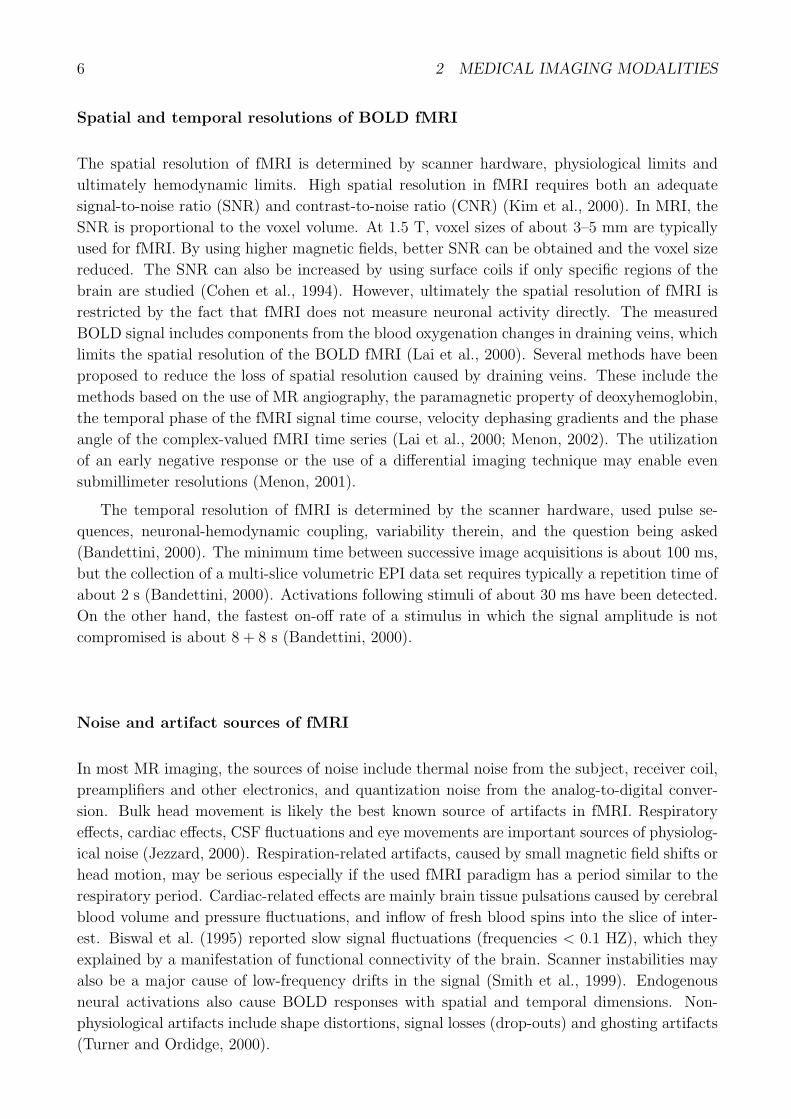
Spatial and temporal resolutions of BOLD fMRI
The spatial resolution of fMRI is determined by scanner hardware, physiological limits and
ultimately hemodynamic limits. High spatial resolution in fMRI requires both an adequate
signal-to-noise ratio (SNR) and contrast-to-noise ratio (CNR) (Kim et al., 2000). In MRI, the
SNR is proportional to the voxel volume. At 1.5 T, voxel sizes of about 3–5 mm are typically
used for fMRI. By using higher magnetic fields, better SNR can be obtained and the voxel size
reduced. The SNR can also be increased by using surface coils if only specific regions of the
brain are studied (Cohen et al., 1994). However, ultimately the spatial resolution of fMRI is
restricted by the fact that fMRI does not measure neuronal activity directly. The measured
BOLD signal includes components from the blood oxygenation changes in draining veins, which
limits the spatial resolution of the BOLD fMRI (Lai et al., 2000). Several methods have been
proposed to reduce the loss of spatial resolution caused by draining veins. These include the
methods based on the use of MR angiography, the paramagnetic property of deoxyhemoglobin,
the temporal phase of the fMRI signal time course, velocity dephasing gradients and the phase
angle of the complex-valued fMRI time series (Lai et al., 2000; Menon, 2002). The utilization
of an early negative response or the use of a differential imaging technique may enable even
submillimeter resolutions (Menon, 2001).
The temporal resolution of fMRI is determined by the scanner hardware, used pulse se-
quences, neuronal-hemodynamic coupling, variability therein, and the question being asked
(Bandettini, 2000). The minimum time between successive image acquisitions is about 100 ms,
but the collection of a multi-slice volumetric EPI data set requires typically a repetition time of
about 2 s (Bandettini, 2000). Activations following stimuli of about 30 ms have been detected.
On the other hand, the fastest on-off rate of a stimulus in which the signal amplitude is not
compromised is about 8 + 8 s (Bandettini, 2000).
Noise and artifact sources of fMRI
In most MR imaging, the sources of noise include thermal noise from the subject, receiver coil,
preamplifiers and other electronics, and quantization noise from the analog-to-digital conver-
sion. Bulk head movement is likely the best known source of artifacts in fMRI. Respiratory
effects, cardiac effects, CSF fluctuations and eye movements are important sources of physiolog-
ical noise (Jezzard, 2000). Respiration-related artifacts, caused by small magnetic field shifts or
head motion, may be serious especially if the used fMRI paradigm has a period similar to the
respiratory period. Cardiac-related effects are mainly brain tissue pulsations caused by cerebral
blood volume and pressure fluctuations, and inflow of fresh blood spins into the slice of inter-
est. Biswal et al. (1995) reported slow signal fluctuations (frequencies < 0.1 HZ), which they
explained by a manifestation of functional connectivity of the brain. Scanner instabilities may
also be a major cause of low-frequency drifts in the signal (Smith et al., 1999). Endogenous
neural activations also cause BOLD responses with spatial and temporal dimensions. Non-
physiological artifacts include shape distortions, signal losses (drop-outs) and ghosting artifacts
(Turner and Ordidge, 2000).
7
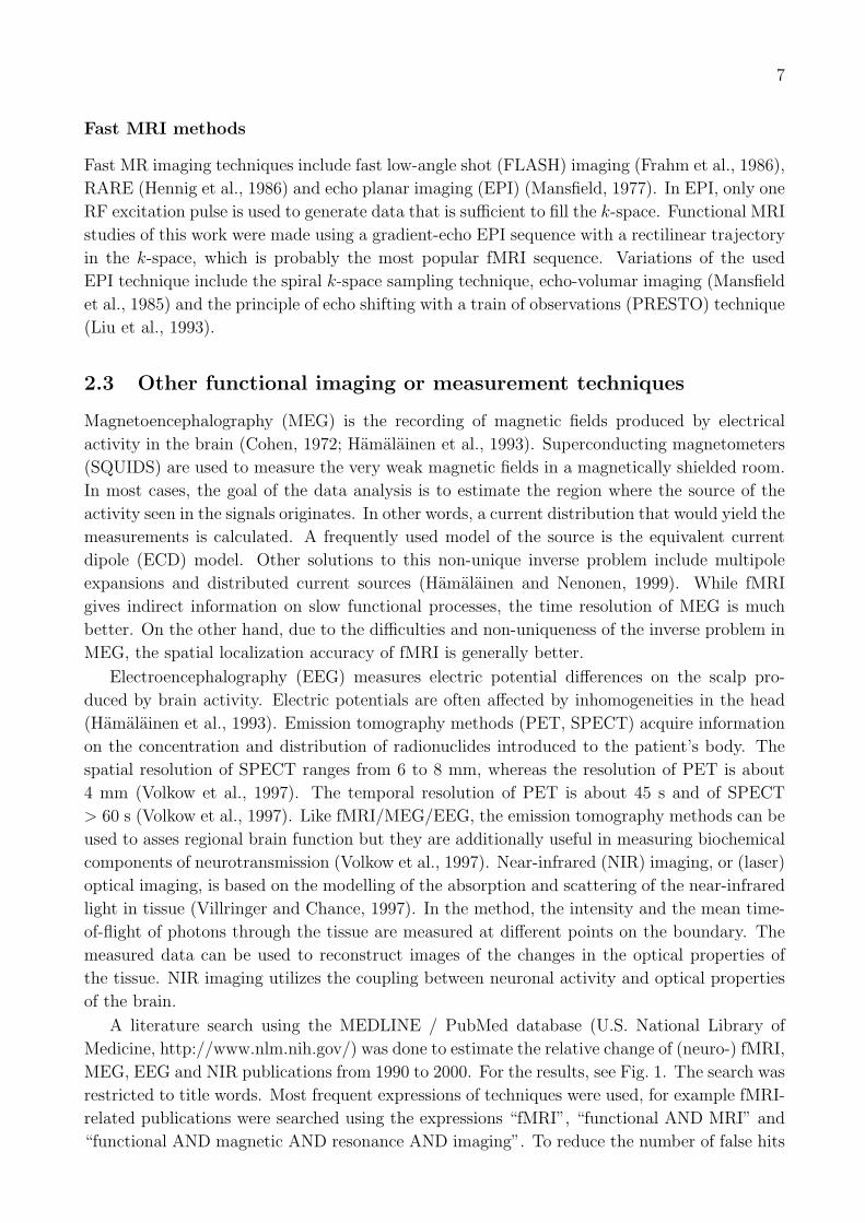
Fast MRI methods
Fast MR imaging techniques include fast low-angle shot (FLASH) imaging (Frahm et al., 1986),
RARE (Hennig et al., 1986) and echo planar imaging (EPI) (Mansfield, 1977). In EPI, only one
RF excitation pulse is used to generate data that is sufficient to fill the k-space. Functional MRI
studies of this work were made using a gradient-echo EPI sequence with a rectilinear trajectory
in the k-space, which is probably the most popular fMRI sequence. Variations of the used
EPI technique include the spiral k-space sampling technique, echo-volumar imaging (Mansfield
et al., 1985) and the principle of echo shifting with a train of observations (PRESTO) technique
(Liu et al., 1993).
2.3 Other functional imaging or measurement techniques
Magnetoencephalography (MEG) is the recording of magnetic fields produced by electrical
activity in the brain (Cohen, 1972; Hamalainen et al., 1993). Superconducting magnetometers
(SQUIDS) are used to measure the very weak magnetic fields in a magnetically shielded room.
In most cases, the goal of the data analysis is to estimate the region where the source of the
activity seen in the signals originates. In other words, a current distribution that would yield the
measurements is calculated. A frequently used model of the source is the equivalent current
dipole (ECD) model. Other solutions to this non-unique inverse problem include multipole
expansions and distributed current sources (Hamalainen and Nenonen, 1999). While fMRI
gives indirect information on slow functional processes, the time resolution of MEG is much
better. On the other hand, due to the difficulties and non-uniqueness of the inverse problem in
MEG, the spatial localization accuracy of fMRI is generally better.
Electroencephalography (EEG) measures electric potential differences on the scalp pro-
duced by brain activity. Electric potentials are often affected by inhomogeneities in the head
(Hamalainen et al., 1993). Emission tomography methods (PET, SPECT) acquire information
on the concentration and distribution of radionuclides introduced to the patient’s body. The
spatial resolution of SPECT ranges from 6 to 8 mm, whereas the resolution of PET is about
4 mm (Volkow et al., 1997). The temporal resolution of PET is about 45 s and of SPECT
> 60 s (Volkow et al., 1997). Like fMRI/MEG/EEG, the emission tomography methods can be
used to asses regional brain function but they are additionally useful in measuring biochemical
components of neurotransmission (Volkow et al., 1997). Near-infrared (NIR) imaging, or (laser)
optical imaging, is based on the modelling of the absorption and scattering of the near-infrared
light in tissue (Villringer and Chance, 1997). In the method, the intensity and the mean time-
of-flight of photons through the tissue are measured at different points on the boundary. The
measured data can be used to reconstruct images of the changes in the optical properties of
the tissue. NIR imaging utilizes the coupling between neuronal activity and optical properties
of the brain.
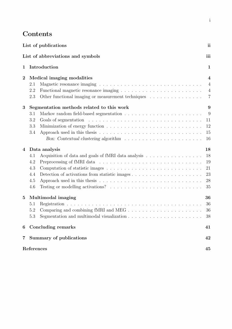
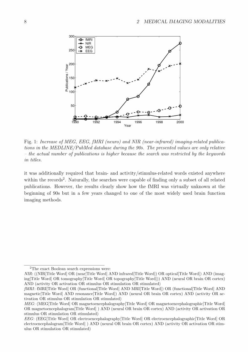
A literature search using the MEDLINE / PubMed database (U.S. National Library of
Medicine, http://www.nlm.nih.gov/) was done to estimate the relative change of (neuro-) fMRI,
MEG, EEG and NIR publications from 1990 to 2000. For the results, see Fig. 1. The search was
restricted to title words. Most frequent expressions of techniques were used, for example fMRI-
related publications were searched using the expressions “fMRI”, “functional AND MRI” and
“functional AND magnetic AND resonance AND imaging”. To reduce the number of false hits
8 2 MEDICAL IMAGING MODALITIES
1990 1992 1994 1996 1998 20000
50
100
150
200
250
300
Year
Pub
licat
ions
/ Y
ear
fMRINIRMEGEEG
Fig. 1: Increase of MEG, EEG, fMRI (neuro) and NIR (near-infrared) imaging-related publica-tions in the MEDLINE/PubMed database during the 90s. The presented values are only relative– the actual number of publications is higher because the search was restricted by the keywordsin titles.
it was additionally required that brain- and activity/stimulus-related words existed anywhere
within the records2. Naturally, the searches were capable of finding only a subset of all related
publications. However, the results clearly show how the fMRI was virtually unknown at the
beginning of 90s but in a few years changed to one of the most widely used brain function
imaging methods.
2The exact Boolean search expressions were:NIR: ((NIR[Title Word] OR (near[Title Word] AND infrared[Title Word]) OR optical[Title Word]) AND (imag-ing[Title Word] OR tomography[Title Word] OR topography[Title Word])) AND (neural OR brain OR cortex)AND (activity OR activation OR stimulus OR stimulation OR stimulated)fMRI : fMRI[Title Word] OR (functional[Title Word] AND MRI[Title Word]) OR (functional[Title Word] ANDmagnetic[Title Word] AND resonance[Title Word]) AND (neural OR brain OR cortex) AND (activity OR ac-tivation OR stimulus OR stimulation OR stimulated)MEG : (MEG[Title Word] OR magnetoencephalography[Title Word] OR magnetoencephalographic[Title Word]OR magnetoencephalogram[Title Word] ) AND (neural OR brain OR cortex) AND (activity OR activation ORstimulus OR stimulation OR stimulated)EEG : (EEG[Title Word] OR electroencephalography[Title Word] OR electroencephalographic[Title Word] ORelectroencephalogram[Title Word] ) AND (neural OR brain OR cortex) AND (activity OR activation OR stim-ulus OR stimulation OR stimulated)
9
3 Segmentation methods related to this work
By definition, segmentation means that an image is divided into non-overlapping (disjoint)
objects in a meaningful way. Classification of each pixel or voxel of an image to one of the
possible classes results in a segmented image. The number of different segmentation methods
developed for medical images is huge. Some of the methods used in medical imaging were
reviewed by Clarke et al. (1995) and by Acharya and Menon (1998). There are also several
ways to classify the methods. One way is to divide the methods into non-contextual and
contextual methods. In non-contextual methods, the voxel’s classification does not depend on
the measurement values of other voxels. A voxel is classified using only the measurement vector
of the voxel under consideration. In the case of one-channel data, this is called one-level or
multi-level thresholding. Contextual methods utilize information from other voxels, especially
from the adjacent voxels. Another criterion divides segmentation methods into those that
use an a priori model about the expected segmentation and those which do not. Geometry-
driven methods use an a priori geometric model, which is deformed using edge information and
elasticity constraints [for a review see e.g. Acharya and Menon (1998) and for an application
see Lotjonen et al. (1999)]. The Markov random field models (MRF) are another approach to
incorporate a contextual a priori model to the segmentation. The idea behind MRF models is
outlined in the next subsection.
3.1 Markov random field-based segmentation
It is usually reasonable to assume that the distribution of class labelling at a voxel is conditioned
on the class labels in the other voxels. Especially, it is likely that the true classification of nearby
voxels is strongly correlated. This prior assumption can be modelled by Markov random fields
(MRFs) (Besag, 1974; Geman and Geman, 1984), which are widely used in segmentation and
noise reduction tasks. Besag (1986) introduced the iterated conditional modes (ICM) algorithm
that is a computationally efficient method to carry out MRF-based segmentation. A similar
algorithm was used by Kittler and Pairman (1985) to identify clouds. What is important to
note is that these algorithms use both the measurement value of a voxel and classification
information from the neighborhood simultaneously. Information from larger neighborhoods is
incorporated by iterating the classification. The method developed in this thesis follows these
ideas and is closely related to the ICM algorithm. Pappas (1992) presented a general MRF-
based segmentation algorithm that took into account local intensity variations by an iterative
procedure involving averaging over a sliding window whose size decreased as the algorithm
progressed. Liang et al. (1994) segmented brain images using a Markov random field prior and 3-
channel data including T1-, T2- and PD-weighted 2-D MR images. Unlike in many other papers,
the number of classes was estimated from the data. Park and Kurz (1996) developed a general
MRF-based image enhancement algorithm and found that it outperformed e.g. the median
filter. Held et al. (1997) described a fully automatic 3-D segmentation technique for brain MR
images. Implementations based on simulated annealing and ICM were presented. Difference to
the method by Liang et al. (1994) was that also intensity inhomogeneities and non-parametric
intensity distributions were taken into account, but the classes were pre-determined. Rajapakse
et al. utilized a 3-D MRF model in the segmentation of single-channel magnetic resonance (MR)
cerebral images (Rajapakse et al., 1997; Rajapakse and Kruggel, 1998). Their method was also
10 3 SEGMENTATION METHODS RELATED TO THIS WORK
adaptive to intensity inhomogeneities, but in addition MRF-parameters were estimated from
the data. Also Kim and Paik (1998) presented an unsupervised segmentation method for MR
images. Their method was based on an adaptive version of the ICM algorithm, and even the
size of the window for parameter estimation was chosen using the data. Descombes et al.
(1998b,a) proposed reduction of noise from fMRI datasets using an MRF model. Van Leemput
et al. (1999) described a fully automatic brain tissue classification method. In their approach,
initialization is done using a digital brain atlas containing prior expectations about the spatial
location of tissue classes. Thereafter, tissue classification including correction for MR signal
inhomogeneities and parameter estimation is done in an interleaved manner by maximizing
tissue likelihood in the presence of MRF-prior.
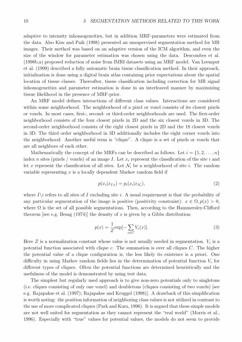
An MRF model defines interactions of different class values. Interactions are considered
within some neighborhood. The neighborhood of a pixel or voxel consists of its closest pixels
or voxels. In most cases, first-, second- or third-order neighborhoods are used. The first-order
neighborhood consists of the four closest pixels in 2D and the six closest voxels in 3D. The
second-order neighborhood consists of the eight closest pixels in 2D and the 18 closest voxels
in 3D. The third order neighborhood in 3D additionally includes the eight corner voxels into
the neighborhood. Another useful term is “clique”. A clique is a set of pixels or voxels that
are all neighbors of each other.
Mathematically the concept of the MRFs can be described as follows. Let i = 1, 2, . . . , nindex n sites (pixels / voxels) of an image I. Let xi represent the classification of the site i and
let x represent the classification of all sites. Let Ni be a neighborhood of site i. The random
variable representing x is a locally dependent Markov random field if
p(xi|xI\i) = pi(xi|xNi), (2)
where I\i refers to all sites of I excluding site i. A usual requirement is that the probability of
any particular segmentation of the image is positive (positivity constraint): x ∈ Ω, p(x) > 0,
where Ω is the set of all possible segmentations. Then, according to the Hammersley-Clifford
theorem [see e.g. Besag (1974)] the density of x is given by a Gibbs distribution:
p(x) =1
Zexp[−
∑c∈C
Vc(x)]. (3)
Here Z is a normalization constant whose value is not usually needed in segmentation. Vc is a
potential function associated with clique c. The summation is over all cliques C. The higher
the potential value of a clique configuration is, the less likely its existence is a priori. One
difficulty in using Markov random fields lies in the determination of potential function Vc for
different types of cliques. Often the potential functions are determined heuristically and the
usefulness of the model is demonstrated by using test data.
The simplest but regularly used approach is to give non-zero potentials only to singletons
(i.e. cliques consisting of only one voxel) and doubletons (cliques consisting of two voxels) [see
e.g. Rajapakse et al. (1997); Rajapakse and Kruggel (1998)]. A drawback of this simplification
is worth noting: the position information of neighboring class values is not utilized in contrast to
the use of more complicated cliques (Park and Kurz, 1996). It is argued that these simple models
are not well suited for segmentation as they cannot represent the “real world” (Morris et al.,
1996). Especially with “true” values for potential values, the models do not seem to provide
11
enough “smoothing”, but may delete fine structures. On the other hand, these models have
been used successfully in many applications. The problems can be avoided at least partially by
defining additional restrictions for the potential functions. The use of more complicated models
[e.g. the line and fine structures preserving chien model with 3× 3 cliques by Descombes et al.
(1995)] in segmentation is rare, possibly due to the computational difficulties, which may be
severe in 3D.
The potentials of the singletons (often expressed using α) reflect the a priori knowledge of
the relative likelihood of the different classes. If the a priori likelihood of different classes is
not used (e.g. the classes are assumed to be equally likely), the potentials of the singletons
are set to zero. The potentials of the doubletons (β) are used to adjust the likelihood that
neighboring voxels belong to different classes. One method is to set the potential to β if
the voxels belong to different classes and otherwise to 0 or −β [e.g. Besag (1986); Pappas
(1992)]. Sometimes different potentials (β1, β2, . . .) are defined to the first-order, second-order
etc. neighbors [e.g. Rajapakse et al. (1997); Rajapakse and Kruggel (1998); Liang et al. (1994)].
Also possible different voxel dimensions in x−, y−, and z−directions can be taken into account
by defining different interactions for different directions. Sometimes it is useful to order the
classes and define the potentials to utilize this order information. For example, a larger potential
could be given for cliques consisting of white matter (WM) and cerebral spinal fluid (CSF)
voxels than for cliques consisting of gray matter (GM) voxels in place of CSF voxels. This
would reflect prior knowledge that GM voxels are often located between WM and CSF voxels.
Another example is noise reduction using an MRF model. In this case, the potential function
can be defined to be a function of difference of intensity values inside a clique (Park and Kurz,
1996). It is worth noting that an MRF model is often not expected to be an accurate model
of the true image itself but a tool to utilize contextual information. Hence, even if the Markov
a priori model is not accurately determined, its use may significantly improve segmentation
results.
3.2 Goals of segmentation
A frequent goal of segmentation is to choose the most probable segmentation x (maximizing
a posteriori probability, MAP segmentation) given the measurement data and the available a
priori information. Let vector z contain the measurement values, or some other features, of
voxels. Thus, by Bayes’ theorem x maximizes the probability
P (x|z) ∝ p(z|x)p(x). (4)
Another goal of segmentation might be to maximize the marginal posterior probability (MMP)
at each voxel i. That is, to maximize
P (xi|z) ∝∑xI\i
p(z|x)p(x). (5)
This is equivalent to the minimization of the expected number of erroneously classified voxels
and can be seen as an approximation to MAP. The xi’s can be estimated using the Gibbs
sampler (Geman and Geman, 1984).
It is worth noting that the MAP (or MMP) segmentation requires realistic models about
the data and the estimation of the model parameters. For example, the models used for the
12 3 SEGMENTATION METHODS RELATED TO THIS WORK
segmentation of brain MR images include the non-contextual finite Gaussian mixture model
and the contextual Gaussian hidden MRF model (Zhang et al., 2001). Typically, the unknown
parameters are the means and variances of the Gaussian distributions and MRF parameters like
singleton and doubleton interaction parameters. The inclusion of bias field and partial volume
models introduces additional unknown parameters. The determination of the parameters using
either training data or the actual data is the central issue of many publications. Several meth-
ods like the expectation-maximization algorithm (Dempster et al., 1977; Van Leemput et al.,
1999; Zhang et al., 2001) have been proposed to estimate the parameters. Estimation of the
model parameters is often carried out in an iteratively manner simultaneously with the energy
minimization (see the next subsection) algorithm. We have adopted an alternative approach,
namely the classification by hypothesis testing, not requiring the estimation of parameters.
When the voxels of an image are classified into two classes, ω0 and ω1, there are two basic
types of errors:
• a voxel of class ω0 is erroneously classified to class ω1 and
• a voxel of class ω1 is erroneously classified to class ω0.
Segmentation by hypothesis testing means classification of the voxels into two classes so that
one of the classes is defined as a null class. A voxel is classified to the alternative, or rejection,
class if the null hypothesis is rejected. The null hypothesis is rejected if the probability for
the test statistic, or a higher one, to occur by chance assuming that the null hypothesis is true
is smaller than a predefined α-level. Segmentation by hypothesis testing can be used if the
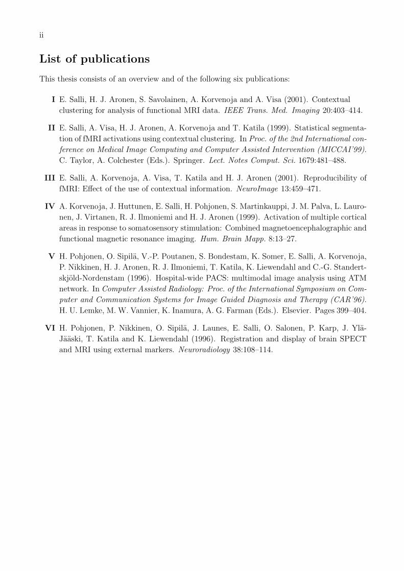
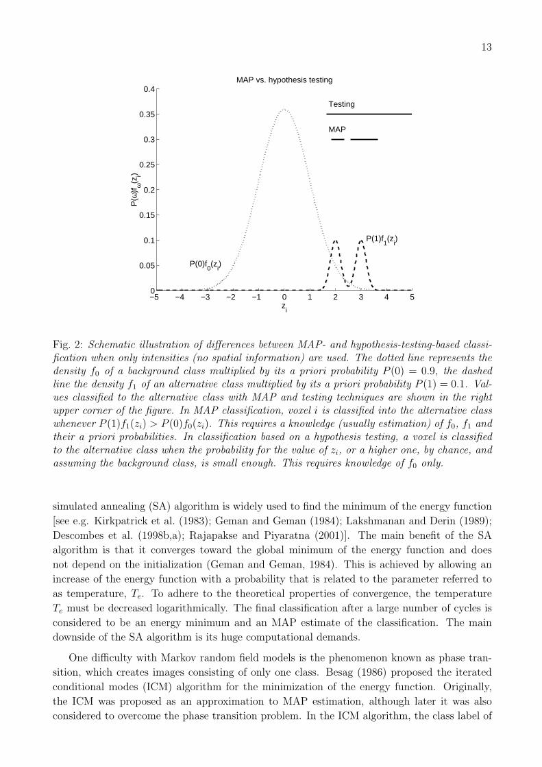
intensity distribution of the null class is known. The difference between MAP- and testing-
based classification is illustrated in Fig. 2. Voxel classification based on hypothesis testing is
widely used in fMRI data analysis because
• the distribution of non-activated voxels can be approximately characterized but the dis-
tribution of activated voxels is unknown,
• the classification of a non-activated voxel to the activation class is considered a more
serious error than the classification of an activated voxel to the non-activation class, and
• the significance (p-) values of the found activated regions are often needed to report the
significance of the findings.
Hypothesis testing is often performed on each voxel separately. Segmentation methodology
and contextual information are seldom used in testing approaches. Generally speaking, the use
of information from other voxels prevents accurate statistical voxel-specific inferences. However,
by properly choosing the segmentation algorithm the advantages may be more important than
the drawbacks.
3.3 Minimization of energy function
The a posteriori probability of segmentation x can be written as P (x|z) ∝ exp− U(x), where
U(x) is called the energy function. Maximization of the a posteriori probability is then equiv-
alent to the minimization of energy function U(x). In practice, the minimization algorithm
determines the labelling of the voxels and is occasionally called the labelling algorithm. A
13
−5 −4 −3 −2 −1 0 1 2 3 4 50
0.05
0.1
0.15
0.2
0.25
0.3
0.35
0.4
MAP
Testing
zi
P(ω
)fω(z
i)
MAP vs. hypothesis testing
P(0)f0(z
i)
P(1)f1(z
i)
Fig. 2: Schematic illustration of differences between MAP- and hypothesis-testing-based classi-fication when only intensities (no spatial information) are used. The dotted line represents thedensity f0 of a background class multiplied by its a priori probability P (0) = 0.9, the dashedline the density f1 of an alternative class multiplied by its a priori probability P (1) = 0.1. Val-ues classified to the alternative class with MAP and testing techniques are shown in the rightupper corner of the figure. In MAP classification, voxel i is classified into the alternative classwhenever P (1)f1(zi) > P (0)f0(zi). This requires a knowledge (usually estimation) of f0, f1 andtheir a priori probabilities. In classification based on a hypothesis testing, a voxel is classifiedto the alternative class when the probability for the value of zi, or a higher one, by chance, andassuming the background class, is small enough. This requires knowledge of f0 only.
simulated annealing (SA) algorithm is widely used to find the minimum of the energy function
[see e.g. Kirkpatrick et al. (1983); Geman and Geman (1984); Lakshmanan and Derin (1989);
Descombes et al. (1998b,a); Rajapakse and Piyaratna (2001)]. The main benefit of the SA
algorithm is that it converges toward the global minimum of the energy function and does
not depend on the initialization (Geman and Geman, 1984). This is achieved by allowing an
increase of the energy function with a probability that is related to the parameter referred to
as temperature, Te. To adhere to the theoretical properties of convergence, the temperature
Te must be decreased logarithmically. The final classification after a large number of cycles is
considered to be an energy minimum and an MAP estimate of the classification. The main
downside of the SA algorithm is its huge computational demands.
One difficulty with Markov random field models is the phenomenon known as phase tran-
sition, which creates images consisting of only one class. Besag (1986) proposed the iterated
conditional modes (ICM) algorithm for the minimization of the energy function. Originally,
the ICM was proposed as an approximation to MAP estimation, although later it was also
considered to overcome the phase transition problem. In the ICM algorithm, the class label of
14 3 SEGMENTATION METHODS RELATED TO THIS WORK
Slice 9 Slice 10 Slice 11 Slice 12 Slice 13
Slice 14 Slice 15 Slice 16 Slice 17 Slice 18
Slice 19 Slice 20 Slice 21 Slice 22 Slice 23
(a)
(b) (c) (d) (e) (f) (g)
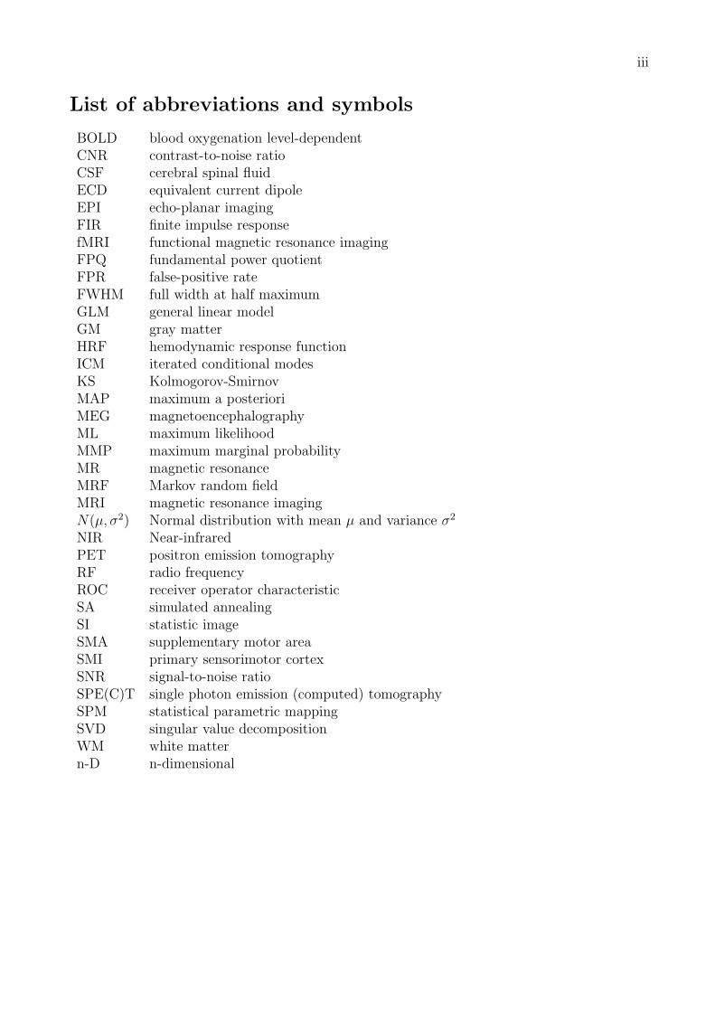
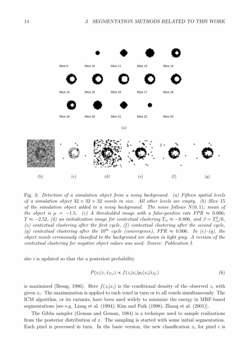
Fig. 3: Detection of a simulation object from a noisy background. (a) Fifteen spatial levelsof a simulation object 32 × 32 × 32 voxels in size. All other levels are empty. (b) Slice 15of the simulation object added to a noisy background. The noise follows N(0, 1); mean ofthe object is µ = −1.5. (c) A thresholded image with a false-positive rate FPR ≈ 0.006;T ≈ −2.52, (d) an initialization image for contextual clustering Tcc ≈ −0.806, and β = T 2
cc/6,(e) contextual clustering after the first cycle, (f) contextual clustering after the second cycle,(g) contextual clustering after the 10th cycle (convergence), FPR ≈ 0.006. In (c)–(g), theobject voxels erroneously classified to the background are shown in light gray. A version of thecontextual clustering for negative object values was used. Source: Publication I.
site i is updated so that the a posteriori probability
P (xi|z, xI\i) ∝ f(zi|xi)pi(xi|xNi) (6)
is maximized (Besag, 1986). Here f(zi|xi) is the conditional density of the observed zi with
given xi. The maximization is applied to each voxel in turn or to all voxels simultaneously. The
ICM algorithm, or its variants, have been used widely to minimize the energy in MRF-based
segmentations [see e.g. Liang et al. (1994); Kim and Paik (1998); Zhang et al. (2001)].
The Gibbs sampler (Geman and Geman, 1984) is a technique used to sample realizations
from the posterior distribution of x. The sampling is started with some initial segmentation.
Each pixel is processed in turn. In the basic version, the new classification xi for pixel i is
15
−10
−8
−6
−4
−2
0
2
4
6
8
10
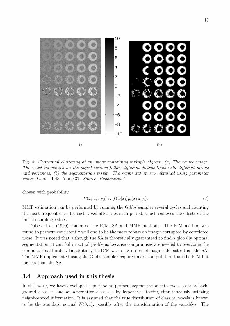
(a) (b)
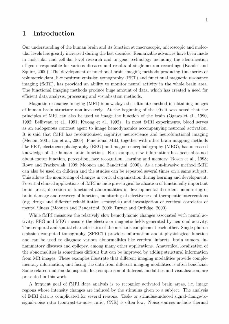
Fig. 4: Contextual clustering of an image containing multiple objects. (a) The source image.The voxel intensities on the object regions follow different distributions with different meansand variances, (b) the segmentation result. The segmentation was obtained using parametervalues Tcc ≈ −1.48, β ≈ 0.37. Source: Publication I.
chosen with probability
P (xi|z, xI\i) ∝ f(zi|xi)pi(xi|xNi). (7)
MMP estimation can be performed by running the Gibbs sampler several cycles and counting
the most frequent class for each voxel after a burn-in period, which removes the effects of the
initial sampling values.
Dubes et al. (1990) compared the ICM, SA and MMP methods. The ICM method was
found to perform consistently well and to be the most robust on images corrupted by correlated
noise. It was noted that although the SA is theoretically guaranteed to find a globally optimal
segmentation, it can fail in actual problems because compromises are needed to overcome the
computational burden. In addition, the ICM was a few orders of magnitude faster than the SA.
The MMP implemented using the Gibbs sampler required more computation than the ICM but
far less than the SA.
3.4 Approach used in this thesis
In this work, we have developed a method to perform segmentation into two classes, a back-
ground class ω0 and an alternative class ω1, by hypothesis testing simultaneously utilizing
neighborhood information. It is assumed that the true distribution of class ω0 voxels is known
to be the standard normal N(0, 1), possibly after the transformation of the variables. The
16 3 SEGMENTATION METHODS RELATED TO THIS WORK
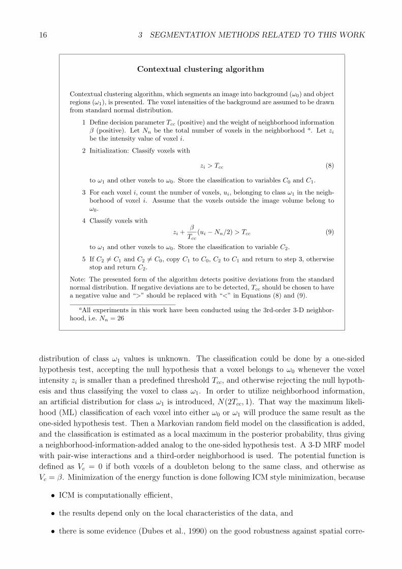
Contextual clustering algorithm
Contextual clustering algorithm, which segments an image into background (ω0) and objectregions (ω1), is presented. The voxel intensities of the background are assumed to be drawnfrom standard normal distribution.
1 Define decision parameter Tcc (positive) and the weight of neighborhood informationβ (positive). Let Nn be the total number of voxels in the neighborhood a. Let zi
be the intensity value of voxel i.
2 Initialization: Classify voxels with
zi > Tcc (8)
to ω1 and other voxels to ω0. Store the classification to variables C0 and C1.
3 For each voxel i, count the number of voxels, ui, belonging to class ω1 in the neigh-borhood of voxel i. Assume that the voxels outside the image volume belong toω0.
4 Classify voxels with
zi +β
Tcc(ui −Nn/2) > Tcc (9)
to ω1 and other voxels to ω0. Store the classification to variable C2.
5 If C2 6= C1 and C2 6= C0, copy C1 to C0, C2 to C1 and return to step 3, otherwisestop and return C2.
Note: The presented form of the algorithm detects positive deviations from the standardnormal distribution. If negative deviations are to be detected, Tcc should be chosen to havea negative value and “>” should be replaced with “<” in Equations (8) and (9).
aAll experiments in this work have been conducted using the 3rd-order 3-D neighbor-hood, i.e. Nn = 26
distribution of class ω1 values is unknown. The classification could be done by a one-sided
hypothesis test, accepting the null hypothesis that a voxel belongs to ω0 whenever the voxel
intensity zi is smaller than a predefined threshold Tcc, and otherwise rejecting the null hypoth-
esis and thus classifying the voxel to class ω1. In order to utilize neighborhood information,
an artificial distribution for class ω1 is introduced, N(2Tcc, 1). That way the maximum likeli-
hood (ML) classification of each voxel into either ω0 or ω1 will produce the same result as the
one-sided hypothesis test. Then a Markovian random field model on the classification is added,
and the classification is estimated as a local maximum in the posterior probability, thus giving
a neighborhood-information-added analog to the one-sided hypothesis test. A 3-D MRF model
with pair-wise interactions and a third-order neighborhood is used. The potential function is
defined as Vc = 0 if both voxels of a doubleton belong to the same class, and otherwise as
Vc = β. Minimization of the energy function is done following ICM style minimization, because
• ICM is computationally efficient,
• the results depend only on the local characteristics of the data, and
• there is some evidence (Dubes et al., 1990) on the good robustness against spatial corre-
17
lations in the noise term.
We will call the segmentation carried out using the ideas presented a “contextual clustering”.
Its steps are summarized in the box, for details of the derivation see Publication I. Segmentation
of a single object from random noise is illustrated in Fig. 3. Segmentation of several objects
following different distributions is shown in Fig. 4. It is worth noting that the algorithm
measures deviation from the background only (i.e. no information about object distributions
is used). In addition, apart from the immediate neighborhood of object voxels, type I error
probabilities are determined by the parameters of the algorithm (Tcc and β) only.
The essential difference between the ICM algorithm (or MAP estimation) and the proposed
algorithm is worth noting. In the ICM, relative a posteriori probabilities for a voxel belonging
to classes ω0 and ω1 should be estimated. A voxel is classified to a class whose a posteriori
probability is the highest. This requires a priori information about the statistical properties
of both classes and parameter estimation. In our approach, only the statistical properties of
background class ω0 are used. Loosely speaking, a voxel is classified to ω1 if the values of the
voxel and the “surrounding” voxels differ enough from the distribution of class ω0. For this
reason, the need for the modelling of activation distributions is avoided. In the derivation from
the ICM, the “real” activation class was replaced with an artificial test class. The mean of the
test class and the interaction between neighboring voxels are set so that a desired overall or
voxel-level type I error rate is achieved, i.e. the mean and MRF parameters no longer represent
the characteristics of the true image. We emphasize that the replacement is a heuristic step.
Hence, relatively extensive tests were conducted in Publications I–III. Main results of the tests
are presented in section 4.
18 4 DATA ANALYSIS
4 Data analysis
4.1 Acquisition of data and goals of fMRI data analysis
In fMRI activation studies a stimulus is given to a subject or the subject is asked to perform
a task. Time series of MR images are recorded and analyzed. In epoch-based, or block-based
fMRI, blocks of different states (e.g. control and stimulus) are alternated and the images of
different states are compared. Each block typically consists of several images. Too short blocks
are inefficient due to the slowness of the hemodynamic response. On the other hand, too long
blocks should be avoided due to baseline fluctuations, subject’s movements and discomfort.
Optimal block length and other parameters of the study designs are debated questions and out
of the scope of this thesis.
In addition to epoch-type studies, fMRI can be used to study event-related activations
(Buckner et al., 1996; Rosen et al., 1998). Event-related fMRI is used to study responses to short
stimuli, e.g. to single words. Event-related task paradigms can be used to map hemodynamic
changes lasting in the order of seconds or several hundreds of milliseconds. Event-related fMRI
provides the ability to study the same paradigms in both fMRI and MEG (or EEG) sessions.
The number of articles related to the fMRI data analysis is large [see e.g. Lange (2000)].
Perhaps the most common goal of fMRI data analysis is to localize the brain areas responsible
for the processing of the stimulus. In many approaches, the localization of fMRI activations
consists of three phases:
1) Preprocessing of the data, possibly including motion correction and smoothing or noise
reduction,
2) voxel-by-voxel computation of the statistic image (SI), also called a statistical (paramet-
ric) map, and
3) segmentation of the SI into activated and non-activated regions.
Phase 2) essentially reduces the 4-D spatio-temporal fMRI data into a 3-D spatial image by
considering all time series separately. The values of the SI follow a known null distribution in
non-activated voxels. Phase 3) is usually called a testing phase aiming to detect statistically
significant activations from the 3-D SI. As will be later discussed, this phase is usually carried
out so that the probabilities of false activation detection (“false-positive rates (FPR)”) are
controlled either at the voxel level or the overall (volume) level. The term “segmentation”
is used here to emphasize that, at least implicitly, the ultimate goal is not only to obtain
information about the location of activation centers but also to obtain other information like
the shapes or sizes of the activations. The simplest approach to segment SI is to threshold it
in a voxel-by-voxel manner. However, it is generally accepted that the truly activated voxels
tend to form clusters, and methods to incorporate spatial information during step 3) have been
developed. We shall describe later in this overview how the contextual clustering procedure
described in section 3 can be used to perform phase 3).
This thesis will concentrate on the localization and delineation of activations. However,
several other questions may be posed than just where the activation happened. Bayesian
models with Markov Chain Monte Carlo posterior sampling seem useful in estimating many
hemodynamic parameters, for example signal rise times or the impact of changing task demands
19
(Genovese, 2000; Gossl et al., 2001). Path analysis is used to quantify relationships between
multiple brain regions (Bullmore et al., 1996b, 2000). The goal of time series clustering [see e.g.
Baumgartner et al. (1997); Golay et al. (1998); Baune et al. (1999); Goutte et al. (1999); Ngan
and Hu (1999)] is to partition the time series into clusters of similar time courses. Typically,
time series clustering does not require prior assumptions about the shape of the expected time
course.
Multivariate analysis, like singular value decomposition (SVD) and independent components
analysis (ICA) (McKeown et al., 1998), take place on all voxels’ time courses at the same time.
SVD, or related principal component analysis (PCA), may be used to explore fMRI-signal
structures without any a priori knowledge about the activation signal [e.g. Bullmore et al.
(1996b); Lange (2000)]. As an example, Friston et al. (1994a) used SVD to extract a global
representation of the hemodynamic response function.
4.2 Preprocessing of fMRI data
Reliable activation detection and the controlling of false-positive rates (FPRs) in fMRI activa-
tion detection requires modelling of noise. Noise can be divided into systematic and random
noise. Optimal detection of activations requires a correct model for the hemodynamic response.
Both the noise and hemodynamic response have temporal and spatial aspects.
The simplest approximation for the time courses of a non-activated voxel is that the intensity
values are independently drawn from a Gaussian distribution with some mean µ and variance
σ2, constant over the experiment. In an approximation, the time courses are also spatially
independent if the means are not considered. This white Gaussian noise model is often implicitly
assumed in the widely used t-test methods. In practice, the intensity values of fMRI data are
correlated in time and space. The amount of correlation may depend, e.g., on the size of voxels
and the time of repetition. The number of false-positive detections may differ from the expected
number of false positives if the correlations are not taken into account properly. In addition, the
changes in the baseline level cause substantial difficulties in the data analysis. Spatial aspects
are closely related to the activation detection phase and are hence deferred to subsection 4.4.
The primary reason for low-pass filtering in statistical analysis is to set the degrees of
freedom of the data to a known level. In addition, running a filter whose width corresponds to
the width of the signal increases detection sensitivity. Kruggel et al. (1999) compared a moving
average filter, an FIR low-pass filter, an autoregressive filter and a Kalman filter with event-
related data. The best sensitivity was determined for the moving average filter, closely followed
by the temporal low-pass filter. However, the low-pass filter revealed a higher independence
of the results in relation to the filter parameters. Zarahn et al. (1997) reported that temporal
autocorrelation in spatially unsmoothed data is described well by a 1/f relationship, where f
is frequency. In addition, they found that temporal smoothing of the noise data with low-pass
filters in conjunction with the use of a general linear model (GLM) (Worsley and Friston, 1995)
was advantageous in controlling FPRs.
Systematic noise, like drifts and fluctuations, may be caused, e.g., by scanner instabilities,
scanner noise, motion artifacts, variations in blood pressure and respiratory or cardiac effects
(Bandettini et al., 1998; Smith et al., 1999). A standard approach is to high-pass filter the time
series or simply remove a linear trend. The high-pass filtering can be performed as a separate
pre-processing step or it can incorporated to the linear model discussed later. Biswal et al.
20 4 DATA ANALYSIS
(1996) described the use of finite impulse response (FIR) band reject digital filters in removing
physiological fluctuations. Buonocore and Maddock (1997) developed an adaptive Wiener filter
to suppress cardiac and respiratory structure noise in fMRI images. Skudlarski et al. (1999)
found that removal of intensity drifts using high-pass filtering is beneficial to the efficacy of the
analysis. Marchini and Ripley (2000) removed non-linear trends by using a simple running-lines
smoother, which they found to be a reliable method.
A global nuisance signal can be partially taken into account by scaling the images, so that
they all have the same global mean value. However, it is possible that much of the brain truly
responds neurally to the experimental paradigm and that adjustment for the global signal leads
to inferences about brain function based on artifact (Aguirre et al., 1998b). The global signal
can also be included as a nuisance covariate into the GLM (Zarahn et al., 1997).
In order to optimize the sensitivity of activation detection, the hemodynamic response
function (HRF) should be modelled accurately. It is generally known that the hemodynamic
response is slow. After the onset of neural activation, it increases to a peak value during several
seconds. Return to the baseline is even slower. Several models have been used for the HRF.
In using the Fourier transform technique, only the frequency of the activation needs to
be known (Bandettini et al., 1993). The same is true when a linear combination of sine and
cosine terms at the fundamental frequency of simulation is fitted (Bullmore et al., 1996a) to the
data. These approaches are naturally limited to the periodic stimulus functions. A widely used
approach is to use a model of a linear and time-invariant system, although it is generally known
that the model is not precisely correct. For example Dale and Buckner (1997) demonstrated that
the fMRI signal summated approximately linearly in visual stimulation experiments although
subtle departures from linearity were observed. In the epoch-based experiments, the linearity
is not as important issue as it is when short stimuli are repeated rapidly. In the linear model
the response to an arbitrary input (stimulus) function is equal to the convolution of that input
with the system’s impulse response. Then, the observed fMRI signal x(t) (without baseline) at
time t in a discrete-time domain is given by
x(t) = α∑s
h(t− s)p(s) + ε(t), (10)
where α is the gain of the fMRI imaging process, p(s) is the stimulus function, h(t) is the
impulse response function and ε(t) represents additive noise. Assuming that the effects of
stimuli summate linearly, this equation can be applied not only to a single stimulus but also to
cases where many stimuli are presented rapidly. The simplest model for the impulse response
function is the delta function. Then x(t) is modelled to be α + ε(t) during a stimulus and ε(t)
otherwise. A slightly more realistic approach is to add a delay of few seconds to the system.
These models are implicitly used in the two-sample t-test. In more advanced approaches, the
impulse response function is modelled by a gamma or Poisson density function (Friston et al.,
1994b; Boynton et al., 1996; Cohen, 1997), a difference between two gamma density functions
(Friston et al., 1998), a Gaussian function (Rajapakse et al., 1998), or an empirically derived
function. Variation in the impulse response (e.g. variation in lag and and dispersion) can be
modelled by a combination of basis functions or by a finite-impulse response (FIR) set. Choices
for the basis function include a canonical response function and its derivatives (Friston et al.,
1998), a Fourier set (Josephs et al., 1997) and gamma density functions (Dale and Buckner,
1997). The FIR sets do not assume any shape for the hemodynamic response, although it is
21
possible to include knowledge about the responses using restriction matrices (Burock and Dale,
2000). In the linear model, it is also possible to define different impulse response functions to
different types of stimuli.
Movement correction and other geometrical transformations
Movement of a subject is considered to be one of the most serious problems in fMRI experiments.
Movement may lead to decreased detection sensitivity or movement artifacts. Often the head of
the patient or volunteer is fixed with a vacuum pillow during scanning. Also bite bars are used.
However, small movements cannot be avoided. To remove the effect of head movements, several
motion correction algorithms based on the internal properties of the data and either rigid or
non-rigid models have been developed and used. The movement correction, as registration in
general, encompasses several separate problems. These include the selection of a cost function,
optimization of the cost function and interpolation of the data after the determination of the
transformation parameters (Woods et al., 1992; Friston et al., 1996b; Eddy et al., 1996; Kim
et al., 1999; Cox and Jesmanowicz, 1999; Jenkinson and Smith, 2001a).
Movement correction is an example of within modality, within subject registration proce-
dure. Several other registration and transformation procedures are also needed in the analysis
of functional data [see e.g. Jenkinson and Smith (2001b)]. In order to show activation maps
on the top of high-resolution structural MR images, a between modalities within subject reg-
istration is widely used. In this case raw functional MR data (e.g. EPI) is registered with the
structural images because the computed activation maps are not suitable for registration. In
some cases, slice position and orientation information from the headers of image files can be
used and registration can be avoided. There is also often a need to combine between modalities
within subject, and between subjects within modality transformations in order to show the
activation maps of different subjects on the top of one common reference image. Difficulty lies
in the fact that substantial variation between anatomies exists. Generally, one of the subjects
is chosen as a reference. Structural images of other subjects are elastically registered with the
reference subject. Then the functional images of each subject are registered with the corre-
sponding structural images of the subject. Finally, the two transformations are combined and
activation maps are transformed to the coordinates of the reference structural image. Alter-
natively, some standard atlas, like the coordinate system of Talairach and Tournoux (1984),
can be used as a reference coordinate system. This has the advantages that the results can
be reported in standard generally known coordinates and compared easily with other studies.
Additional references concerning the geometrical transformations include Pelizzari et al. (1989);
Thompson and Toga (1996); Christensen et al. (1997); Ashburner et al. (1999).
4.3 Computation of statistic images
In the most basic fMRI analysis technique, the mean of images acquired during one condition is
subtracted from the mean of images acquired during an alternative condition. Images obtained
at the beginning of each epoch are generally discarded due to the delay in the hemodynamic
response. However, the subtraction technique alone does not give information about the sta-
tistical significance of the difference. Instead of direct subtraction, statistic images (SIs) are
preferred. In the SI, non-activated voxels follow a known null distribution. There are several
22 4 DATA ANALYSIS
ways to compute such images.
The SI of t-statistic can be obtained from a subtraction image by normalizing it with the
standard error estimate, i.e. using the methodology of standard Student’s t-tests. The t-statistic
has been used from the early days of fMRI (Constable et al., 1993). In the correlation analysis
(Bandettini et al., 1993), correlation coefficients are calculated between the measured signal
and an expected response function (reference signal) at each voxel. Thereafter, the calculated
correlation coefficients are compared with the theoretical null distribution coefficients. Several
variations exist. Kleinschmidt et al. (1995) used correlation coefficient maps with noise distri-
bution reconstructed from the actual data. Kuppusamy et al. (1997) used a combination of
cross-correlation and t-test images. An example of spectral density estimation methods is a
non-parametric technique described by Marchini and Ripley (2000). The method was found to
be more resistant to high-frequency artifacts than the usual time-domain approaches.
The t-test and the correlation test are special cases of the general linear model (GLM)
(Friston et al., 1995). Usually, the GLM is written in matrix form:
xi = Gbi + εi (11)
Here xi includes measured data for voxel i, G is called a design matrix, bi is a vector of
unknown model parameters, and εi is a vector of residuals drawn from a Gaussian distribution.
The design matrix G models the experiment, e.g. the hemodynamic response (see section 4.2),
baseline, and nuisance effects, like low-frequency components. The columns of G represent
different parts of the model and each row represents one scan (3-D volume). If G is full rank,
the least squares and simultaneously the maximum likelihood (ML) estimates of b are given by
bi = (GT G)−1GT xi, (12)
where T indicates the transpose and −1 the inverse of a matrix. In the case that the data are
convolved (smoothed) using a convolution kernel K, the GLM is written as
Kxi = KGbi + Kei. (13)
Unbiased estimators for bi, its variance and statistical significance were given by Worsley and
Friston (1995). For example,
bi = (GT KT KG)−1GT KT Kxi. (14)
The primary goal of smoothing is to set the temporal autocorrelations to a known level so
that SIs can be computed properly. An alternative approach to the temporal smoothing is to
estimate and remove the actual autocorrelations (pre-whiten the data) (Bullmore et al., 1996a;
Burock and Dale, 2000; Woolrich et al., 2001). Woolrich et al. (2001) found their pre-whitening
approach to give valid statistics at the voxel level and to maximize estimation efficiency.
In order to test a specific effect at voxel i (e.g., is b1,i significantly larger than zero?), a t-
statistic value is calculated. The t-statistic value is calculated by dividing a contrast (i.e. linear
compound of the parameter estimates) by the estimated standard error at the voxel [for details,
see Friston et al. (1995); Worsley and Friston (1995)]. When there is no specific effect at the
voxel, the t-value is drawn from a null distribution, which is, in theory, a t-distribution. All
t-statistic values displayed together form a t-statistic image. The t-statistic images can be
23
transformed to standard z-statistic images using the transformation Φ(t) = Ψ(z), where Φ(·)is the t-distribution function and Ψ(·) is the cumulative standard Gaussian function. The
knowledge about the null distribution enables the determination of voxels in which the specific
effect is statistically significant. The next subsection covers this issue in greater detail. In
addition to t-statistic, also an F -statistic is widely used with the GLM. An F -test can be used
to assess the significance of a subset of basis functions. The F -test allows comparison of the
different factors to the model.
Other statistics are used, too. For example, Bullmore et al. (1996a) presented a test statistic
called a fundamental power quotient (FPQ). In the approach, an fMRI signal is modelled by
the sum of a fitted sine wave and a cosine wave. The FPQ at a voxel is given by
FPQ =1
2
( γ
σ
)2
+
(δ
σ
)2 , (15)
where γ and δ are estimates of the amplitude of a sine wave and a cosine wave, respectively,
and σ is an estimate of the assumed common standard error of γ and δ. In theory, 2 × FPQ
has approximately the chi-squared null distribution with two degrees of freedom.
Ardekani et al. (1999) proposed the use of subspace modelling and maximum likelihood
estimation in the detection of fMRI activations. This method identifies both the dimension
and the basis vectors of the nuisance subspace (confounds) using an ML estimation method.
The Kolmogorov-Smirnov (KS) statistic is widely used in the analysis of fMRI data, [for
a list of publications see Aguirre et al. (1998a)]. The KS-statistic is based on the maximum
distance between the cumulative probability distributions of the different conditions. It does
not assume that the noise in the fMRI time series follows a Gaussian distribution. However,
independence of the samples is assumed. Indeed, experiments indicate that FPRs, yielded by
the KS-test, may excess the tabular values (Aguirre et al., 1998a).
4.4 Detection of activations from statistic images
The ultimate goal of fMRI data analysis is often the detection, localization and delineation
of activation regions from SIs. The approaches can be roughly divided into two groups:
hypothesis-testing-based methods and modelling-based methods. The hypothesis-testing-based
methods control FPRs and detect statistically significantly activated regions. In modelling- or
estimation-based methods, activation distributions are estimated and voxels are classified by
maximizing the a posteriori probabilities.
Spatial smoothness and smoothing
Spatial smoothness, or coherency, i.e. the presence of cross-correlations of voxel time series is
an important issue due to the need for multiple comparison correction. One type of smoothness
can be modelled by a continuously differentiable spatial autocovariance function (Zarahn et al.,
1997). Filtering the data with a Gaussian kernel creates this type of smoothness. The width
of the filter kernel is often expressed with the term of full width at half maximum (FWHM).
An alternative expression is the standard deviation of the filter, λ. For a Gaussian filter, these
24 4 DATA ANALYSIS
two are related according to formula
λ =FWHM√
8ln2. (16)
Spatial smoothing of data with a Gaussian filter is a debated issue. It is argued that the best
smoothing filter is one that matches the objects to be identified (Worsley and Friston, 1995).
However, it should be noted that only the detection of objects is considered then. If other as-
pects, like the localization of the edges of objects, are considered, the issue is more complex. It is
generally known that spatial smoothing may dislocate edges and fuse neighboring objects. The
second reason for spatial smoothing is that statistical inferences and multiple comparison correc-
tion utilizing the theory of Gaussian random fields, implemented as SPM’99 software (Wellcome
Department of Cognitive Neurology, London, UK, http://www.fil.ion.ucl.ac.uk/spm/), assume
that the data are spatially smooth (Worsley and Friston, 1995). A Gaussian random field is
one that has a Gaussian distribution at every point and at every collection of points. To fulfill
the smooth Gaussian random field requirement, the fMRI data are smoothed using a Gaus-
sian filter. Several methods for the estimation of the level of smoothness have been developed
(Worsley et al., 1992; Kiebel et al., 1999; Forman et al., 1995). Typically, the methods are
based on the variance of the gradients in statistic or residual images. In multi-subject analysis,
smoothing is used to ensure that effects between subjects are assessed on a reasonable spatial
scale with respect to functional anatomy.
Generally, SIs calculated from heavily smoothed data are able to find large areas of weak
activation, while SIs calculated from unsmoothed or lightly smoothed data are sensitive to
small but strong foci and also to noise. Multifiltering approaches are proposed to find both
types of activations. Poline and Mazoyer (1994) proposed a multiscale method in which the
(PET) image is filtered successively with Gaussian filters of increasing widths. Skudlarski et al.
(1999) studied a modification in which SIs obtained from smoothed data were added to the
SI obtained from unsmoothed data. Also this simpler approach was found to be powerful in
practice.
Descombes et al. (1998a) replaced the Gaussian filtering with an spatio-temporal edge pre-
serving MRF-based noise reduction in order to avoid blurring and to preserve the resolution
of data. Kruggel et al. (1999) compared a finite impulse response temporal low-pass filter, a
temporal Gaussian filter, an autoregressive filter, a spatial Gaussian filter and a spatio-temporal
MRF-based noise reduction. The best shape recovery and sensitivity were obtained using an
MRF filter while the temporal low-pass filter and temporal Gaussian filters provided better
linearity. However, the consequences of MRF data restoration to the statistics of the following
ordinary voxel-by-voxel data analysis remain unclear. Descombes et al. (1998b) extended the
model. A hemodynamic function was estimated for each voxel. A voxel was considered active
if the norm of the hemodynamic function was high enough. MRF potentials were used to reg-
ularize the activation maps, using potentials between the activation map and parameter maps
that characterize the hemodynamic functions.
Hypothesis testing
In the hypothesis-testing-based approaches, it is tested whether the null hypothesis can be
rejected with some statistical significance level (called false-positive rate (FPR), α-level of test
25
or probability of type I error). When a statistical test is applied separately for each voxel,
the total number of tests for typical fMRI data is thousands. Hence, the overall probability of
finding at least one statistically significant voxel is considerably larger than the level chosen for
conducting each individual test. This is called a multiple comparison problem. One method to
control overall (family-wise) FPRs is Bonferroni correction. Specifically, to do k tests, one for
each voxel, the overall α-level is divided by k to obtain the required voxel-level α-level. The
drawback of the Bonferroni correction is that the smoothness of the data may lead to the too
conservative thresholds.
Different procedures are different in sensitivity, localization power and delineation accuracy.
Omnibus tests (Friston et al., 1991) have no localization power at all. If an omnibus test rejects
the null hypothesis, no information about the location of activations is obtained. The procedure
is said to control the overall FPR in the weak sense (Friston et al., 1996a). For example, a
test that is based on the total number of voxels above some threshold is an omnibus test.
High localization power and strong control is obtained by making statistical inferences for each
voxel separately. Then, the voxels above some intensity threshold are considered activated. A
procedure is said to control the FPR in the strong sense if the probability of a false positive
over any set of voxels for which the null hypothesis is true is less than α regardless of the truth
of the null hypothesis elsewhere.
Various post-processing operations can be used after the thresholding. By using spatial
extent thresholds, the intensity threshold can be lowered, still maintaining a low overall FPR
(Friston et al., 1994b). Simple median filtering can be used to eliminate spurious small activa-
tions. In a modification called neighborhood filtering (Skudlarski et al., 1999), only the voxels
that have a sufficient number of activated neighbors are left to the activation map. However,
Skudlarski et al. found that spatial smoothing of images is more efficient than extent thresh-
olding or neighborhood filtering of the SI. Kleinschmidt et al. (1995) heuristically combined
spatial information to the correlation coefficient analysis. The spatial extent of activations was
delineated by adding neighboring pixels with lower correlation coefficient values.
The approaches to control FPRs and to make multiple comparison correction can be di-
vided into theoretical parametric approaches, non-parametric approaches and simulation-based
approaches (Petersson, 1998).
Theoretical parametric approaches. Theoretical parametric approaches are based on
Gaussian field approximation. To hold the assumptions, the fMRI data are smoothed before
the analysis. Used approximations are only asymptotically true, in the limit of high thresholds.
The results exist for voxel-level, cluster-level and set-level inferences. A basic voxel-level test
gives the probability that the observed voxel value, or a higher one, could have occurred by
chance in the data volume. This probability is commonly called a corrected p-value of the test.
Cluster-level tests give a probability that a connected activation region observed could have
occurred by chance (Worsley et al., 1992; Poline et al., 1997). Friston et al. (1996a) introduced
an analysis to make set-level inferences, i.e. to calculate the probability of getting the observed
number of clusters, or more, in the volume analyzed. Together the voxel-level, cluster-level and
set-level inferences form a hierarchy of tests that have different regional specificity and power.
Non-parametric approaches. The permutation test theory can be used to detect activa-
tions and to handle multiple comparison problem (Holmes et al., 1996; Belmonte and Yurgelun-
Todd, 2001; Nichols and Holmes, 2002). An advantage of the randomization or permutation
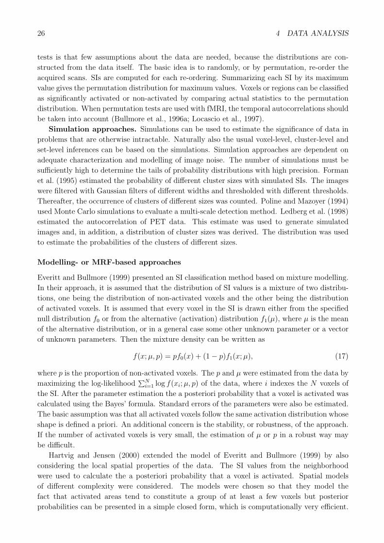
26 4 DATA ANALYSIS
tests is that few assumptions about the data are needed, because the distributions are con-
structed from the data itself. The basic idea is to randomly, or by permutation, re-order the
acquired scans. SIs are computed for each re-ordering. Summarizing each SI by its maximum
value gives the permutation distribution for maximum values. Voxels or regions can be classified
as significantly activated or non-activated by comparing actual statistics to the permutation
distribution. When permutation tests are used with fMRI, the temporal autocorrelations should
be taken into account (Bullmore et al., 1996a; Locascio et al., 1997).
Simulation approaches. Simulations can be used to estimate the significance of data in
problems that are otherwise intractable. Naturally also the usual voxel-level, cluster-level and
set-level inferences can be based on the simulations. Simulation approaches are dependent on
adequate characterization and modelling of image noise. The number of simulations must be
sufficiently high to determine the tails of probability distributions with high precision. Forman
et al. (1995) estimated the probability of different cluster sizes with simulated SIs. The images
were filtered with Gaussian filters of different widths and thresholded with different thresholds.
Thereafter, the occurrence of clusters of different sizes was counted. Poline and Mazoyer (1994)
used Monte Carlo simulations to evaluate a multi-scale detection method. Ledberg et al. (1998)
estimated the autocorrelation of PET data. This estimate was used to generate simulated
images and, in addition, a distribution of cluster sizes was derived. The distribution was used
to estimate the probabilities of the clusters of different sizes.
Modelling- or MRF-based approaches
Everitt and Bullmore (1999) presented an SI classification method based on mixture modelling.
In their approach, it is assumed that the distribution of SI values is a mixture of two distribu-
tions, one being the distribution of non-activated voxels and the other being the distribution
of activated voxels. It is assumed that every voxel in the SI is drawn either from the specified
null distribution f0 or from the alternative (activation) distribution f1(µ), where µ is the mean
of the alternative distribution, or in a general case some other unknown parameter or a vector
of unknown parameters. Then the mixture density can be written as
f(x; µ, p) = pf0(x) + (1− p)f1(x; µ), (17)
where p is the proportion of non-activated voxels. The p and µ were estimated from the data by
maximizing the log-likelihood∑N
i=1 log f(xi; µ, p) of the data, where i indexes the N voxels of
the SI. After the parameter estimation the a posteriori probability that a voxel is activated was
calculated using the Bayes’ formula. Standard errors of the parameters were also be estimated.
The basic assumption was that all activated voxels follow the same activation distribution whose
shape is defined a priori. An additional concern is the stability, or robustness, of the approach.
If the number of activated voxels is very small, the estimation of µ or p in a robust way may
be difficult.
Hartvig and Jensen (2000) extended the model of Everitt and Bullmore (1999) by also
considering the local spatial properties of the data. The SI values from the neighborhood
were used to calculate the a posteriori probability that a voxel is activated. Spatial models
of different complexity were considered. The models were chosen so that they model the
fact that activated areas tend to constitute a group of at least a few voxels but posterior
probabilities can be presented in a simple closed form, which is computationally very efficient.
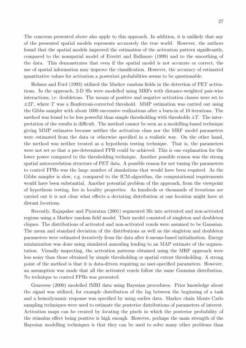
27
The concerns presented above also apply to this approach. In addition, it is unlikely that any
of the presented spatial models represents accurately the true world. However, the authors
found that the spatial models improved the estimation of the activation pattern significantly,
compared to the nonspatial model of Everitt and Bullmore (1999) and to the smoothing of
the data. This demonstrates that even if the spatial model is not accurate or correct, the
use of spatial information may improve the classification. However, the accuracy of estimated
quantitative values for activation a posteriori probabilities seems to be questionable.
Holmes and Ford (1993) utilized the Markov random fields in the detection of PET activa-
tions. In the approach, 2-D SIs were modelled using MRFs with distance-weighted pair-wise
interactions, i.e. doubletons. The means of positive and negative activation classes were set to
±2T , where T was a Bonferroni-corrected threshold. MMP estimation was carried out using
the Gibbs sampler with about 1000 successive realizations after a burn-in of 10 iterations. The
method was found to be less powerful than simple thresholding with thresholds ±T . The inter-
pretation of the results is difficult. The method cannot be seen as a modelling-based technique
giving MMP estimates because neither the activation class nor the MRF model parameters
were estimated from the data or otherwise specified in a realistic way. On the other hand,
the method was neither treated as a hypothesis testing technique. That is, the parameters
were not set so that a pre-determined FPR could be achieved. This is one explanation for the
lower power compared to the thresholding technique. Another possible reason was the strong
spatial autocorrelation structure of PET data. A possible reason for not tuning the parameters
to control FPRs was the large number of simulations that would have been required. As the
Gibbs sampler is slow, e.g. compared to the ICM-algorithm, the computational requirements
would have been substantial. Another potential problem of the approach, from the viewpoint
of hypothesis testing, lies in locality properties. As hundreds or thousands of iterations are
carried out it is not clear what effects a deviating distribution at one location might have at
distant locations.
Recently, Rajapakse and Piyaratna (2001) segmented SIs into activated and non-activated
regions using a Markov random field model. Their model consisted of singleton and doubleton
cliques. The distributions of activated and non-activated voxels were assumed to be Gaussian.
The mean and standard deviation of the distributions as well as the singleton and doubleton
parameters were estimated iteratively from the data after k-means-based initialization. Energy
minimization was done using simulated annealing leading to an MAP estimate of the segmen-
tation. Visually inspecting, the activation patterns obtained using the MRF approach were
less noisy than those obtained by simple thresholding or spatial extent thresholding. A strong
point of the method is that it is data-driven requiring no user-specified parameters. However,
an assumption was made that all the activated voxels follow the same Gaussian distribution.
No technique to control FPRs was presented.
Genovese (2000) modelled fMRI data using Bayesian procedures. Prior knowledge about
the signal was utilized, for example distribution of the lag between the beginning of a task
and a hemodynamic response was specified by using earlier data. Markov chain Monte Carlo
sampling techniques were used to estimate the posterior distributions of parameters of interest.
Activation maps can be created by locating the pixels in which the posterior probability of
the stimulus effect being positive is high enough. However, perhaps the main strength of the
Bayesian modelling techniques is that they can be used to solve many other problems than
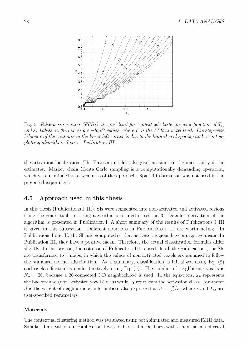
28 4 DATA ANALYSIS
0.1 0.5 1.0 1.5 20.5
11.5
22.5
33.5
44.5
55.5
66.5
77.5
88.5
9
Tcc
s
1
1
1
1.5
1.5
1.5
2
2
22.5
2.5
2.5
3
3
3
3
3.5
3.5
3.5
3.5
4
4
4
4
4.5
4.5
4.5
4.5
5
5
5
5
5.5
5.5
5.5
5.5
6
6
6
6
6
6.5
6.5
6.5
6.5
7
7
7
7
7
Fig. 5: False-positive rates (FPRs) at voxel level for contextual clustering as a function of Tcc
and s. Labels on the curves are −logP values, where P is the FPR at voxel level. The step-wisebehavior of the contours in the lower left corner is due to the limited grid spacing and a contourplotting algorithm. Source: Publication III.
the activation localization. The Bayesian models also give measures to the uncertainty in the
estimates. Markov chain Monte Carlo sampling is a computationally demanding operation,
which was mentioned as a weakness of the approach. Spatial information was not used in the
presented experiments.
4.5 Approach used in this thesis
In this thesis (Publications I–III), SIs were segmented into non-activated and activated regions
using the contextual clustering algorithm presented in section 3. Detailed derivation of the
algorithm is presented in Publication I. A short summary of the results of Publications I–III
is given in this subsection. Different notations in Publications I–III are worth noting. In
Publications I and II, the SIs are computed so that activated regions have a negative mean. In
Publication III, they have a positive mean. Therefore, the actual classification formulas differ
slightly. In this section, the notation of Publication III is used. In all the Publications, the SIs
are transformed to z-maps, in which the values of non-activated voxels are assumed to follow
the standard normal distribution. As a summary, classification is initialized using Eq. (8)
and re-classification is made iteratively using Eq. (9). The number of neighboring voxels is
Nn = 26, because a 26-connected 3-D neighborhood is used. In the equations, ω0 represents
the background (non-activated voxels) class while ω1 represents the activation class. Parameter
β is the weight of neighborhood information, also expressed as β = T 2cc/s, where s and Tcc are
user-specified parameters.
Materials
The contextual clustering method was evaluated using both simulated and measured fMRI data.
Simulated activations in Publication I were spheres of a fixed size with a noncentral spherical
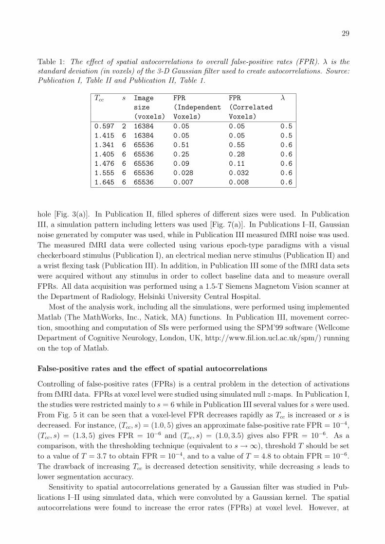
29
Table 1: The effect of spatial autocorrelations to overall false-positive rates (FPR). λ is thestandard deviation (in voxels) of the 3-D Gaussian filter used to create autocorrelations. Source:Publication I, Table II and Publication II, Table 1.
Tcc s Image FPR FPR λsize (Independent (Correlated
(voxels) Voxels) Voxels)
0.597 2 16384 0.05 0.05 0.5
1.415 6 16384 0.05 0.05 0.5
1.341 6 65536 0.51 0.55 0.6
1.405 6 65536 0.25 0.28 0.6
1.476 6 65536 0.09 0.11 0.6
1.555 6 65536 0.028 0.032 0.6
1.645 6 65536 0.007 0.008 0.6
hole [Fig. 3(a)]. In Publication II, filled spheres of different sizes were used. In Publication
III, a simulation pattern including letters was used [Fig. 7(a)]. In Publications I–II, Gaussian
noise generated by computer was used, while in Publication III measured fMRI noise was used.
The measured fMRI data were collected using various epoch-type paradigms with a visual
checkerboard stimulus (Publication I), an electrical median nerve stimulus (Publication II) and
a wrist flexing task (Publication III). In addition, in Publication III some of the fMRI data sets
were acquired without any stimulus in order to collect baseline data and to measure overall
FPRs. All data acquisition was performed using a 1.5-T Siemens Magnetom Vision scanner at
the Department of Radiology, Helsinki University Central Hospital.
Most of the analysis work, including all the simulations, were performed using implemented
Matlab (The MathWorks, Inc., Natick, MA) functions. In Publication III, movement correc-
tion, smoothing and computation of SIs were performed using the SPM’99 software (Wellcome
Department of Cognitive Neurology, London, UK, http://www.fil.ion.ucl.ac.uk/spm/) running
on the top of Matlab.
False-positive rates and the effect of spatial autocorrelations
Controlling of false-positive rates (FPRs) is a central problem in the detection of activations
from fMRI data. FPRs at voxel level were studied using simulated null z-maps. In Publication I,
the studies were restricted mainly to s = 6 while in Publication III several values for s were used.
From Fig. 5 it can be seen that a voxel-level FPR decreases rapidly as Tcc is increased or s is
decreased. For instance, (Tcc, s) = (1.0, 5) gives an approximate false-positive rate FPR = 10−4,
(Tcc, s) = (1.3, 5) gives FPR = 10−6 and (Tcc, s) = (1.0, 3.5) gives also FPR = 10−6. As a
comparison, with the thresholding technique (equivalent to s →∞), threshold T should be set
to a value of T = 3.7 to obtain FPR = 10−4, and to a value of T = 4.8 to obtain FPR = 10−6.
The drawback of increasing Tcc is decreased detection sensitivity, while decreasing s leads to
lower segmentation accuracy.
Sensitivity to spatial autocorrelations generated by a Gaussian filter was studied in Pub-
lications I–II using simulated data, which were convoluted by a Gaussian kernel. The spatial
autocorrelations were found to increase the error rates (FPRs) at voxel level. However, at
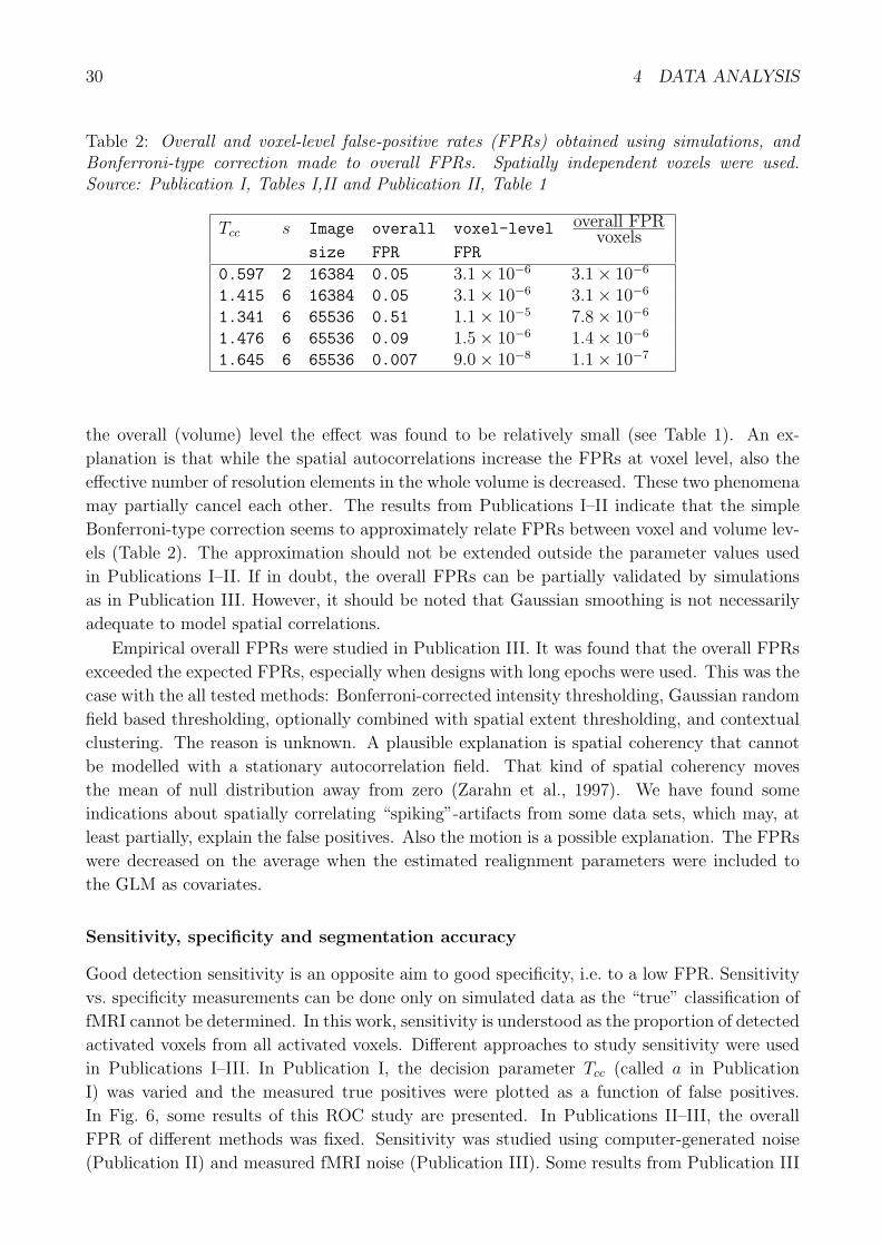
30 4 DATA ANALYSIS
Table 2: Overall and voxel-level false-positive rates (FPRs) obtained using simulations, andBonferroni-type correction made to overall FPRs. Spatially independent voxels were used.Source: Publication I, Tables I,II and Publication II, Table 1
Tcc s Image overall voxel-level overall FPRvoxels
size FPR FPR
0.597 2 16384 0.05 3.1× 10⁻⁶ 3.1× 10⁻⁶
1.415 6 16384 0.05 3.1× 10⁻⁶ 3.1× 10⁻⁶
1.341 6 65536 0.51 1.1× 10⁻⁵ 7.8× 10⁻⁶
1.476 6 65536 0.09 1.5× 10⁻⁶ 1.4× 10⁻⁶
1.645 6 65536 0.007 9.0× 10⁻⁸ 1.1× 10⁻⁷
the overall (volume) level the effect was found to be relatively small (see Table 1). An ex-
planation is that while the spatial autocorrelations increase the FPRs at voxel level, also the
effective number of resolution elements in the whole volume is decreased. These two phenomena
may partially cancel each other. The results from Publications I–II indicate that the simple
Bonferroni-type correction seems to approximately relate FPRs between voxel and volume lev-
els (Table 2). The approximation should not be extended outside the parameter values used
in Publications I–II. If in doubt, the overall FPRs can be partially validated by simulations
as in Publication III. However, it should be noted that Gaussian smoothing is not necessarily
adequate to model spatial correlations.
Empirical overall FPRs were studied in Publication III. It was found that the overall FPRs
exceeded the expected FPRs, especially when designs with long epochs were used. This was the
case with the all tested methods: Bonferroni-corrected intensity thresholding, Gaussian random
field based thresholding, optionally combined with spatial extent thresholding, and contextual
clustering. The reason is unknown. A plausible explanation is spatial coherency that cannot
be modelled with a stationary autocorrelation field. That kind of spatial coherency moves
the mean of null distribution away from zero (Zarahn et al., 1997). We have found some
indications about spatially correlating “spiking”-artifacts from some data sets, which may, at
least partially, explain the false positives. Also the motion is a possible explanation. The FPRs
were decreased on the average when the estimated realignment parameters were included to
the GLM as covariates.
Sensitivity, specificity and segmentation accuracy
Good detection sensitivity is an opposite aim to good specificity, i.e. to a low FPR. Sensitivity
vs. specificity measurements can be done only on simulated data as the “true” classification of
fMRI cannot be determined. In this work, sensitivity is understood as the proportion of detected
activated voxels from all activated voxels. Different approaches to study sensitivity were used
in Publications I–III. In Publication I, the decision parameter Tcc (called a in Publication
I) was varied and the measured true positives were plotted as a function of false positives.
In Fig. 6, some results of this ROC study are presented. In Publications II–III, the overall
FPR of different methods was fixed. Sensitivity was studied using computer-generated noise
(Publication II) and measured fMRI noise (Publication III). Some results from Publication III
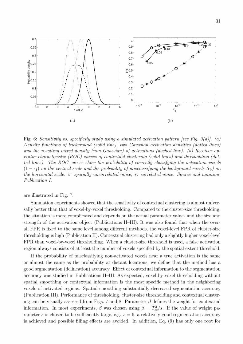
31
−10 −8 −6 −4 −2 0 2 4 60
0.05
0.1
0.15
0.2
0.25
0.3
0.35
0.4
z value
Pro
babi
lity
dens
ity
(a)
10−4
10−3
10−2
10−1
100
0
0.1
0.2
0.3
0.4
0.5
0.6
0.7
0.8
0.9
1
ε0
1−ε 1
0.05
0.090.13
0.21 0.29 0.37
(b)
Fig. 6: Sensitivity vs. specificity study using a simulated activation pattern [see Fig. 3(a)]. (a)Density functions of background (solid line), two Gaussian activation densities (dotted lines)and the resulting mixed density (non-Gaussian) of activations (dashed line). (b) Receiver op-erator characteristic (ROC) curves of contextual clustering (solid lines) and thresholding (dot-ted lines). The ROC curves show the probability of correctly classifying the activation voxels(1− ε1) on the vertical scale and the probability of misclassifying the background voxels (ε0) onthe horizontal scale. : spatially uncorrelated noise; ∗: correlated noise. Source and notation:Publication I.
are illustrated in Fig. 7.
Simulation experiments showed that the sensitivity of contextual clustering is almost univer-
sally better than that of voxel-by-voxel thresholding. Compared to the cluster-size thresholding,
the situation is more complicated and depends on the actual parameter values and the size and
strength of the activation object (Publications II–III). It was also found that when the over-
all FPR is fixed to the same level among different methods, the voxel-level FPR of cluster-size
thresholding is high (Publication II). Contextual clustering had only a slightly higher voxel-level
FPR than voxel-by-voxel thresholding. When a cluster-size threshold is used, a false activation
region always consists of at least the number of voxels specified by the spatial extent threshold.
If the probability of misclassifying non-activated voxels near a true activation is the same
or almost the same as the probability at distant locations, we define that the method has a
good segmentation (delineation) accuracy. Effect of contextual information to the segmentation
accuracy was studied in Publications II–III. As expected, voxel-by-voxel thresholding without
spatial smoothing or contextual information is the most specific method in the neighboring
voxels of activated regions. Spatial smoothing substantially decreased segmentation accuracy
(Publication III). Performance of thresholding, cluster-size thresholding and contextual cluster-
ing can be visually assessed from Figs. 7 and 8. Parameter β defines the weight for contextual
information. In most experiments, β was chosen using β = T 2cc/s. If the value of weight pa-
rameter s is chosen to be sufficiently large, e.g. s = 6, a relatively good segmentation accuracy
is achieved and possible filling effects are avoided. In addition, Eq. (9) has only one root for
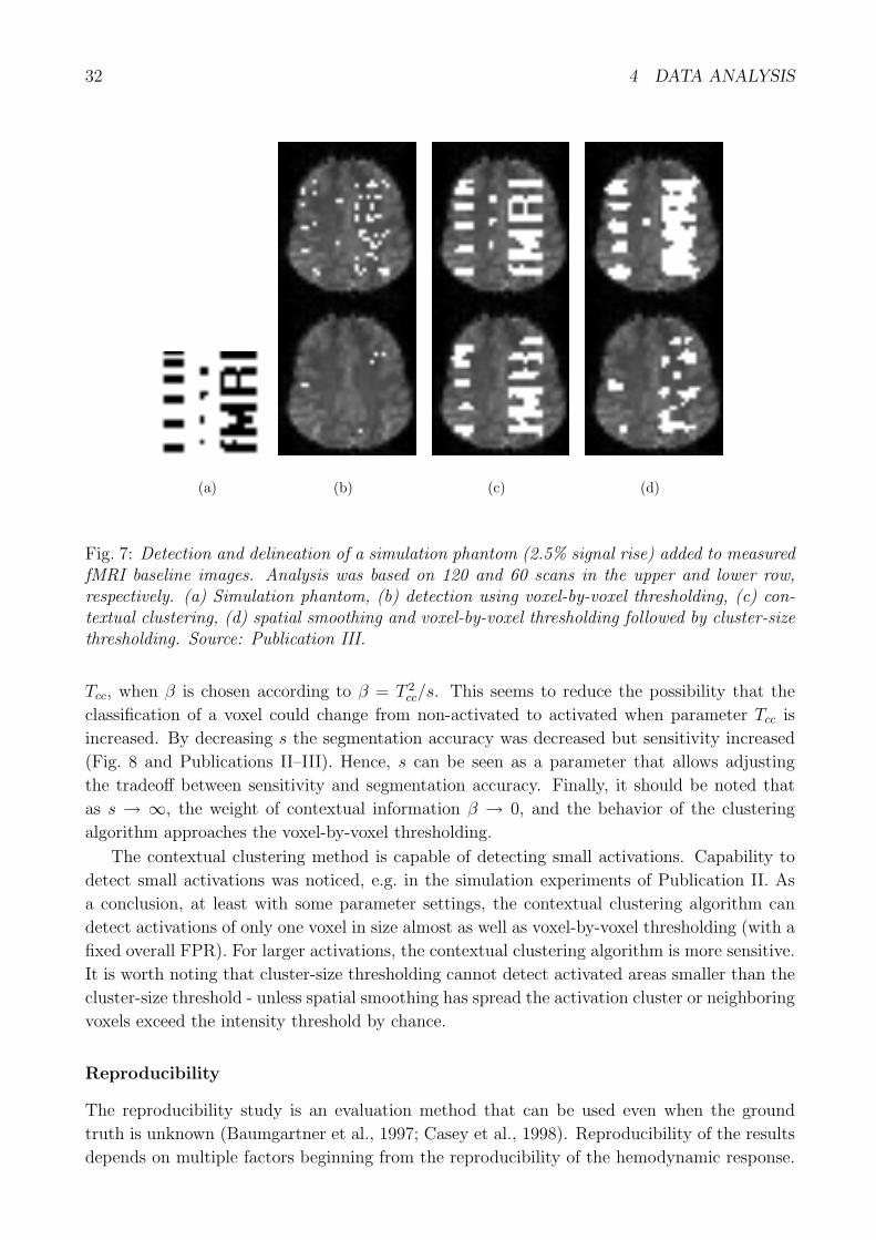
32 4 DATA ANALYSIS
(a) (b) (c) (d)
Fig. 7: Detection and delineation of a simulation phantom (2.5% signal rise) added to measuredfMRI baseline images. Analysis was based on 120 and 60 scans in the upper and lower row,respectively. (a) Simulation phantom, (b) detection using voxel-by-voxel thresholding, (c) con-textual clustering, (d) spatial smoothing and voxel-by-voxel thresholding followed by cluster-sizethresholding. Source: Publication III.
Tcc, when β is chosen according to β = T 2cc/s. This seems to reduce the possibility that the
classification of a voxel could change from non-activated to activated when parameter Tcc is
increased. By decreasing s the segmentation accuracy was decreased but sensitivity increased
(Fig. 8 and Publications II–III). Hence, s can be seen as a parameter that allows adjusting
the tradeoff between sensitivity and segmentation accuracy. Finally, it should be noted that
as s → ∞, the weight of contextual information β → 0, and the behavior of the clustering
algorithm approaches the voxel-by-voxel thresholding.
The contextual clustering method is capable of detecting small activations. Capability to
detect small activations was noticed, e.g. in the simulation experiments of Publication II. As
a conclusion, at least with some parameter settings, the contextual clustering algorithm can
detect activations of only one voxel in size almost as well as voxel-by-voxel thresholding (with a
fixed overall FPR). For larger activations, the contextual clustering algorithm is more sensitive.
It is worth noting that cluster-size thresholding cannot detect activated areas smaller than the
cluster-size threshold - unless spatial smoothing has spread the activation cluster or neighboring
voxels exceed the intensity threshold by chance.
Reproducibility
The reproducibility study is an evaluation method that can be used even when the ground
truth is unknown (Baumgartner et al., 1997; Casey et al., 1998). Reproducibility of the results
depends on multiple factors beginning from the reproducibility of the hemodynamic response.
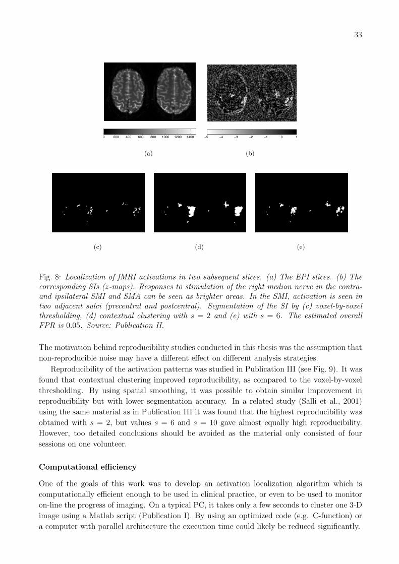
33
0 200 400 600 800 1000 1200 1400
(a)
−5 −4 −3 −2 −1 0 1
(b)
(c) (d) (e)
Fig. 8: Localization of fMRI activations in two subsequent slices. (a) The EPI slices. (b) Thecorresponding SIs (z-maps). Responses to stimulation of the right median nerve in the contra-and ipsilateral SMI and SMA can be seen as brighter areas. In the SMI, activation is seen intwo adjacent sulci (precentral and postcentral). Segmentation of the SI by (c) voxel-by-voxelthresholding, (d) contextual clustering with s = 2 and (e) with s = 6. The estimated overallFPR is 0.05. Source: Publication II.
The motivation behind reproducibility studies conducted in this thesis was the assumption that
non-reproducible noise may have a different effect on different analysis strategies.
Reproducibility of the activation patterns was studied in Publication III (see Fig. 9). It was
found that contextual clustering improved reproducibility, as compared to the voxel-by-voxel
thresholding. By using spatial smoothing, it was possible to obtain similar improvement in
reproducibility but with lower segmentation accuracy. In a related study (Salli et al., 2001)
using the same material as in Publication III it was found that the highest reproducibility was
obtained with s = 2, but values s = 6 and s = 10 gave almost equally high reproducibility.
However, too detailed conclusions should be avoided as the material only consisted of four
sessions on one volunteer.
Computational efficiency
One of the goals of this work was to develop an activation localization algorithm which is
computationally efficient enough to be used in clinical practice, or even to be used to monitor
on-line the progress of imaging. On a typical PC, it takes only a few seconds to cluster one 3-D
image using a Matlab script (Publication I). By using an optimized code (e.g. C-function) or
a computer with parallel architecture the execution time could likely be reduced significantly.
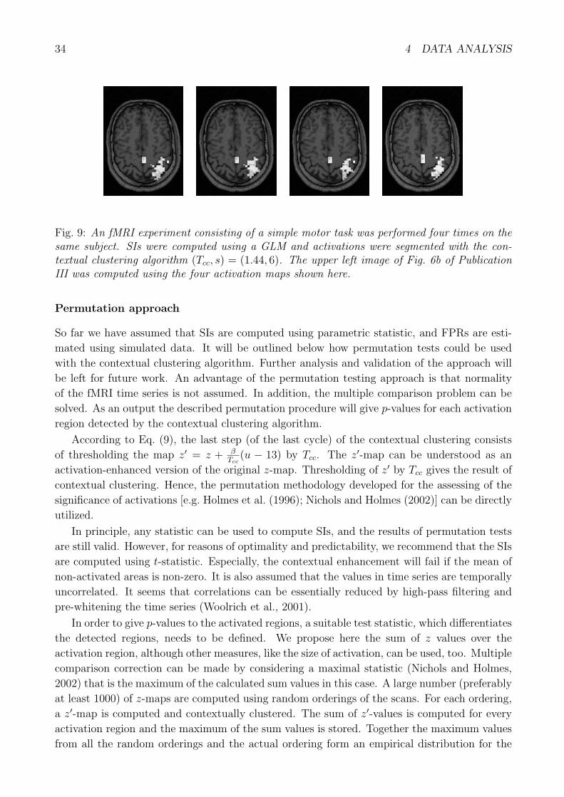
34 4 DATA ANALYSIS
Fig. 9: An fMRI experiment consisting of a simple motor task was performed four times on thesame subject. SIs were computed using a GLM and activations were segmented with the con-textual clustering algorithm (Tcc, s) = (1.44, 6). The upper left image of Fig. 6b of PublicationIII was computed using the four activation maps shown here.
Permutation approach
So far we have assumed that SIs are computed using parametric statistic, and FPRs are esti-
mated using simulated data. It will be outlined below how permutation tests could be used
with the contextual clustering algorithm. Further analysis and validation of the approach will
be left for future work. An advantage of the permutation testing approach is that normality
of the fMRI time series is not assumed. In addition, the multiple comparison problem can be
solved. As an output the described permutation procedure will give p-values for each activation
region detected by the contextual clustering algorithm.
According to Eq. (9), the last step (of the last cycle) of the contextual clustering consists
of thresholding the map z′ = z + βTcc
(u − 13) by Tcc. The z′-map can be understood as an
activation-enhanced version of the original z-map. Thresholding of z′ by Tcc gives the result of
contextual clustering. Hence, the permutation methodology developed for the assessing of the
significance of activations [e.g. Holmes et al. (1996); Nichols and Holmes (2002)] can be directly
utilized.
In principle, any statistic can be used to compute SIs, and the results of permutation tests
are still valid. However, for reasons of optimality and predictability, we recommend that the SIs
are computed using t-statistic. Especially, the contextual enhancement will fail if the mean of
non-activated areas is non-zero. It is also assumed that the values in time series are temporally
uncorrelated. It seems that correlations can be essentially reduced by high-pass filtering and
pre-whitening the time series (Woolrich et al., 2001).
In order to give p-values to the activated regions, a suitable test statistic, which differentiates
the detected regions, needs to be defined. We propose here the sum of z values over the
activation region, although other measures, like the size of activation, can be used, too. Multiple
comparison correction can be made by considering a maximal statistic (Nichols and Holmes,
2002) that is the maximum of the calculated sum values in this case. A large number (preferably
at least 1000) of z-maps are computed using random orderings of the scans. For each ordering,
a z′-map is computed and contextually clustered. The sum of z′-values is computed for every
activation region and the maximum of the sum values is stored. Together the maximum values
from all the random orderings and the actual ordering form an empirical distribution for the
35
maximal statistic. The multiple comparison corrected p-value for each detected activation
region is the proportion of the permutation distribution for the maximal statistic that is greater
than or equal to the sum of z′-values obtained using the actual ordering.
Parameters Tcc and β must be chosen properly to enhance the activation regions. If too
large Tcc is chosen, the activation regions are not enhanced. Similarly, if Tcc is chosen to be too
small, almost all voxels are enhanced, resulting in no actual enhancement for activation regions.
In both cases the results are still statistically valid but it is unlikely that any activations are
detected. The problem here is that Tcc and β need to be chosen before the analysis is performed.
If the t-statistic is used to compute the SIs, the results from the Publications I and III can be
used to set the parameters so that only a small proportion of the voxels is initially classified
as activated. Thereafter, the results from the permutation testing can be used to reject the
activation regions whose p-value is larger than 0.05, for example.
4.6 Testing or modelling activations?
As already discussed, the two fundamentally different ways to classify voxels of fMRI statistic
images into activated and non-activated voxels are
1) by controlling the FPRs (either voxel-level or overall), and
2) by finding a posteriori the most probable segmentation, or by minimizing the total num-
ber of false classifications - both false positives and false negatives. A variation of this
approach would be to minimize the weighted sum of false positives and negatives.
Naturally the goals are loosely defined because the concept “activation” cannot be defined
easily. Traditionally, mostly way 1) has been used in the fMRI activation detection while type
2) classification is widely used i.e. in the brain tissue classification. In this thesis, the way 1)
has been adopted. The primary reason is that the way 1) requires information only about the
distribution of non-activated voxels while the way 2) requires the modelling of the activation
distributions.
Potentially, the modelling of activation distributions could provide a posteriori probabilities
for a voxel being activated or non-activated voxel. However, the modelling of fMRI activation
distributions seems to be a much more complicated issue than e.g. the modelling of different
tissue classes in the segmentation of structural brain MR images. In general, any parametric
forms (e.g. Gaussian or Poisson) for intensity distributions of activations in SIs can hardly be
realistic. It is well possible that fMRI data consist of multiple activation spots. Each of the
spots may have its own distribution. In addition, the distribution of statistic values most likely
vary spatially within each activation spot. Realistic modelling of all these factors would be
important but difficult, considering that the proportion of activated voxels may be very small.
In approach 1) only the distribution of non-activated voxels is required. This information
is provided by the definition of the used statistic. Voxels whose statistic value is high enough
to occur by chance are considered activated. In this section and in Publications I–III it was
demonstrated that spatial context can be used to decrease the effect of random noise and to
increase the probability of detecting weak activations. In addition, the shapes of activations
could be reconstructed relatively accurately in the simulation experiments.
36 5 MULTIMODAL IMAGING
5 Multimodal imaging
Different imaging modalities provide complementary information. The combination of data
acquired using different methods is useful but not straightforward. In this section, some case
studies about combining and comparing structural and functional brain imaging or measure-
ment data are presented. Especially, methods for segmentation, registration, visualization and
comparison of fMRI and MEG localization results are discussed.
5.1 Registration
A basic requirement for multimodal imaging is the registration of different image modalities.
The co-registration between MEG and MRI is not straightforward because MEG does not
provide any anatomic landmarks. In Publications IV–V, a standard procedure based on the
anatomical landmarks (preauricular points and the nasion) was used. These, as well as three
head position indicator coils attached to the skin, were located with a three-dimensional dig-
itizer (Polhemus, Inc., Colchester, VT, USA). The head position within the measurement de-
war was determined using current fed into the indicator coils (Ahlfors and Ilmoniemi, 1989).
Co-registration between MEG and MRI was determined by locating the preauricular points
and nasion from the MR images. The transformation between structural high-resolution MRI
and fMRI activation maps (Publications III–V) was implemented by utilizing slice-positioning
information included into the header files of structural high-resolution MR and functional echo-
planar images. In this approach, it is assumed that the subject has not moved between the
structural MRI and fMRI sessions. It is also assumed that geometrical distortions are not
significantly different between the fMRI and MRI data sets. This is an issue that should be
studied in the future and, if necessary, a distortion correction method may be used. The reg-
istration algorithm used for the MRI and SPECT data (Publication VI) follows a noniterative
least-squares method using a singular value decomposition of a 3× 3 covariance matrix (Arun
et al., 1987). The used approach is based on external skin markers or anatomical markers
defined interactively on the screen using a mouse. After the registration the data sets are in
the same coordinate system and thus comparable.
5.2 Comparing and combining fMRI and MEG
Although MEG is sensitive to millisecond-scale changes in mental activity, its ability to resolve
source localization is limited by the ill-posed inverse problem. PET and especially fMRI have a
higher spatial resolution than MEG but worse temporal resolution. In the context of functional
brain imaging, first attempts to restrict the electromagnetic inverse problem with PET data
were done by Heinze et al. (1994). However, fMRI provides even better spatial resolution
than PET, event-related fMRI techniques providing the possibility to use stimulus setups that
are identical to or slightly modified compared to those used in MEG. There have been several
studies on the regularization of the MEG inverse problem using the physiological and structural
information available from MRI and fMRI [see e.g. George et al. (1995); Liu et al. (1998); Dale
et al. (2000) and Publication IV]. The use of structural MRI can be based on the findings that
the majority of the magnetic signals observed arise from the gray matter. Additionally, the
neurons are preferentially oriented perpendicular to the cortex. This information can be used
37
to constrain the orientation of sources. The usefulness of fMRI arises from the assumption
that at many activations, sources contributing to the MEG signal can be detected with fMRI.
However, it is possible that areas classified as active by fMRI produce no MEG signal (extra
fMRI sources). Conversely, it is possible that some electromagnetically active sources are not
detected by fMRI (invisible fMRI sources). Therefore, the MEG solution space should not be
overconstrained by fMRI data (Liu et al., 1998). Despite some mismatches, combined fMRI,
MRI and MEG data have been successfully used to obtain accurate spatiotemporal maps of
human brain activity, including information about statistical reliability and spatial accuracy at
different locations (Ahlfors et al., 1999; Dale et al., 2000).
In MEG, a common approach to the inverse problem is the modelling of the activation
sources with equivalent current dipoles (ECD). An ECD is the simplest electrical current ele-
ment that could explain the measured magnetic field. In Publication IV, the fMRI data were
used to specify the locations of the ECDs while the time-varying intensity and orientation in-
formation was obtained from MEG. Another approach is to define the locations of all possible
sources a priori and to determine the components of each dipole. As the number of possible
source locations is generally larger than the number of sensors, minimum-norm solutions have
been used. Additionally, fMRI data can be used to weight the possible locations of sources. Liu
et al. (1998) conducted Monte Carlo simulations, studied the usefulness of the approach and
quantified the effects of extra and invisible fMRI sources. Information from the MRI was found
to give an improved solution for the MEG inverse problem with high spatial and temporal
resolution.
In Publication IV, an eight-dipole model fitted to MEG data was constrained with fMRI
data. The MEG data were obtained with the Neuromag-122 magnetometer at the BioMag
Laboratory, Helsinki University Central Hospital. The objectives of the study were
• to compare the localizations obtained with MRI and fMRI separately, and
• to study the time course of activation at different cortical sites.
Related to present thesis, image processing tools for the comparison of the locations of fMRI
and MEG activations were designed and implemented.
To compare the source locations deduced from fMRI and MEG data, the Euclidean distance
between the center points of activations detected by MEG and fMRI was measured. The
location of a fitted current dipole was used directly as a center point of activation in MEG.
In fMRI, an activation region typically consists of a number of voxels. The centroid (i.e. the
center of mass) of an activation area was used to specify the location of the fMRI activation.
This required a method to cluster the activated voxels from the fMRI into separate activation
areas.
The active voxels of thresholded fMRI statistic images were grouped into 6–8 clusters using
the k-means clustering (Bow, 1984). The objective function to be minimized is the sum of
squared distances between each voxel and its cluster center:
S =∑∀i
[i− C(i)]2, (18)
where C(i) is the mean of the cluster that voxel i is assigned to. The initialization was done
manually.
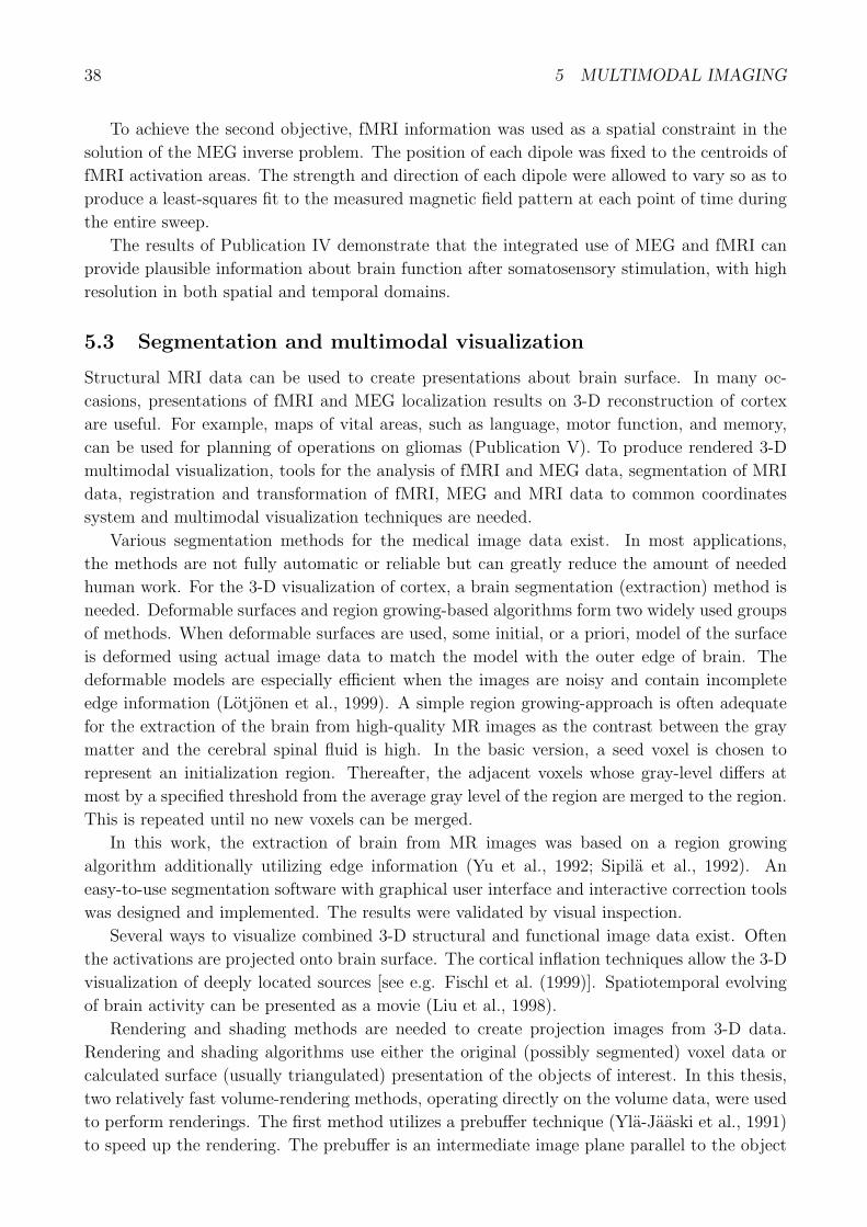
38 5 MULTIMODAL IMAGING
To achieve the second objective, fMRI information was used as a spatial constraint in the
solution of the MEG inverse problem. The position of each dipole was fixed to the centroids of
fMRI activation areas. The strength and direction of each dipole were allowed to vary so as to
produce a least-squares fit to the measured magnetic field pattern at each point of time during
the entire sweep.
The results of Publication IV demonstrate that the integrated use of MEG and fMRI can
provide plausible information about brain function after somatosensory stimulation, with high
resolution in both spatial and temporal domains.
5.3 Segmentation and multimodal visualization
Structural MRI data can be used to create presentations about brain surface. In many oc-
casions, presentations of fMRI and MEG localization results on 3-D reconstruction of cortex
are useful. For example, maps of vital areas, such as language, motor function, and memory,
can be used for planning of operations on gliomas (Publication V). To produce rendered 3-D
multimodal visualization, tools for the analysis of fMRI and MEG data, segmentation of MRI
data, registration and transformation of fMRI, MEG and MRI data to common coordinates
system and multimodal visualization techniques are needed.
Various segmentation methods for the medical image data exist. In most applications,
the methods are not fully automatic or reliable but can greatly reduce the amount of needed
human work. For the 3-D visualization of cortex, a brain segmentation (extraction) method is
needed. Deformable surfaces and region growing-based algorithms form two widely used groups
of methods. When deformable surfaces are used, some initial, or a priori, model of the surface
is deformed using actual image data to match the model with the outer edge of brain. The
deformable models are especially efficient when the images are noisy and contain incomplete
edge information (Lotjonen et al., 1999). A simple region growing-approach is often adequate
for the extraction of the brain from high-quality MR images as the contrast between the gray
matter and the cerebral spinal fluid is high. In the basic version, a seed voxel is chosen to
represent an initialization region. Thereafter, the adjacent voxels whose gray-level differs at
most by a specified threshold from the average gray level of the region are merged to the region.
This is repeated until no new voxels can be merged.
In this work, the extraction of brain from MR images was based on a region growing
algorithm additionally utilizing edge information (Yu et al., 1992; Sipila et al., 1992). An
easy-to-use segmentation software with graphical user interface and interactive correction tools
was designed and implemented. The results were validated by visual inspection.
Several ways to visualize combined 3-D structural and functional image data exist. Often
the activations are projected onto brain surface. The cortical inflation techniques allow the 3-D
visualization of deeply located sources [see e.g. Fischl et al. (1999)]. Spatiotemporal evolving
of brain activity can be presented as a movie (Liu et al., 1998).
Rendering and shading methods are needed to create projection images from 3-D data.
Rendering and shading algorithms use either the original (possibly segmented) voxel data or
calculated surface (usually triangulated) presentation of the objects of interest. In this thesis,
two relatively fast volume-rendering methods, operating directly on the volume data, were used
to perform renderings. The first method utilizes a prebuffer technique (Yla-Jaaski et al., 1991)
to speed up the rendering. The prebuffer is an intermediate image plane parallel to the object
39
Fig. 10: Examples of 3-D multimodal visualizations. (a) Surface-shaded image constructed usingMRI combined with SPECT data on a cut plane in a man with a cerebral infarct (PublicationVI). (b) The location of an MEG current dipole source representing an evoked response forelectric stimulation of the right median nerve (red dipole) and the center of activation shownby fMRI (blue dot) (Publication V). The MEG localizations in (c) and (d) were obtained byrecording the neuromagnetic field in response to an auditory stimulus and by determining thelocation of a current dipole source. In (c) the original MRI data at the depth of an MEGresponse are shown using gray values inside a circle. The center of the circle indicates thelocalization result at the opposite side of the brain in order to visualize cerebral asymmetry.Source: Tiihonen et al. (1998). In (d) a cut plane is used to visualize an MEG localizationresult. Published e.g. in Kaplan-Solms and Solms (2000). In (e) fMRI activations detectedusing contextual clustering [Tcc = 1.3 (red), Tcc = 1.7, Tcc = 2.1, Tcc = 2.5 and Tcc = 2.9(yellow) (s = 6 in all cases)] are visualized on two slice levels.
slices. This technique was used with a gradient shading method based on the surface normal
vectors estimated from a calculated distance map. This approach was used in Publication VI
and Fig. 10(a) of this overview. The second method uses the Stanford VolPack volume renderer
(Lacroute and Levoy, 1994). The Stanford VolPack renderer uses a similar prebuffer technique
as the first method but also includes additional optimization techniques based on pre-computed
data structures. The shading model of the VolPack is based on the surface orientation estimated
from the original 3-D data. Also the partial transparency of the voxels is modelled. This shading
approach was found to give cortex renderings of good quality [Fig. 10(b)-(e)]. In addition to
the used pre-buffer techniques, several other volume rendering acceleration techniques exist,
e.g. the use of “probe” rays (Pyokkimies et al., 2001) can speed-up rendering.
40 5 MULTIMODAL IMAGING
In a neurosurgery application, MRI, fMRI and MEG data are fused for planning of opera-
tions on gliomas, for example. A “brain map” combining the information from these modalities
is produced for a neurosurgeon, aiding the identification of important functional areas of the
brain during the operation. The map consists of surface-shaded 3-D brain images, constructed
from the anatomical MRI. The MEG and/or fMRI localization results are visualized on the
brain surface. On the other hand, combined MRI and SPECT studies may be useful in the
diagnosis of many diseases (Publication VI). Various multimodal 3-D visualization modes are
shown and explained in Fig. 10. While the clinical value of 3-D renderings has been some-
what unclear so far, they will most likely have an important role e.g. in surgery (Shahidi et al.,
1998). In addition, 3-D renderings have proven to be useful in visualizing research results e.g. in
scientific journals.
41
6 Concluding remarks
Aspects related to the analysis of fMRI data and multimodal brain imaging were presented and
discussed in this work. Especially, a new fMRI activation detection and delineation method
utilizing spatial neighborhood information was developed and studied. It was shown how
weak and therefore statistically insignificant activations changed to significant when spatial
information was used. This was achieved without using models for the distribution of activated
voxels or estimating any segmentation parameters.
Many interesting topics were restricted outside this thesis. These include the usefulness
of more complicated potential functions or larger neighborhoods or utilization of anatomical
or topological information. An interesting possibility would be to confine the analysis to the
cortex and to use a surface-based coordinate system [e.g. Fischl et al. (1999); Andrade et al.
(2001)]. Problems specific to multi-subject studies were not discussed either.
A question not addressed is how stimulus-related activation should be defined. Any stimulus
will cause changes in the neural activity (and hemodynamic response) at different locations of
the brain and potentially in very large areas. As the sensitivity of imaging and analysis methods
improve, the volume of statistically significantly activated regions will likely grow. Therefore,
the activation voxels and/or regions detected must be classified to more and less relevant.
Commonly this is done by assigning statistical significance values to the voxels and clusters.
Another approach would be to use, for example, an estimated magnitude of a hemodynamic
response.
The ultimate goal of data analysis should be kept in mind. For example, a neurosurgeon
might be interested in the most likely location of primary motor cortex, or in the list of possible
locations. Both are different problems than the detection and delineation of statistically signifi-
cant activation areas. More research is needed so the that the optimal data analysis procedures
can be found out.
A possible strength of fMRI compared to MEG is the fMRI’s capability to separate activation
regions which are located close to each other. This separation information may be beneficial
when used as prior information in the MEG inverse problem. In this context, it is important
to avoid data smoothing, which may fuse the activated regions together. Hence, the fMRI
activation detection method developed in this thesis may also be useful when fMRI and MEG
information are combined.
42 7 SUMMARY OF PUBLICATIONS
7 Summary of publications
I Contextual clustering for analysis of functional MRI data (IEEE Trans. Med.
Imaging 20:403–414, 2001).
A contextual clustering algorithm was derived and its relation to the Markov random
fields, ICM algorithm and hypothesis testing was explained. By using receiver operator
characteristics (ROC) analysis, voxel-level sensitivity and specificity of the contextual
clustering was studied. Computer-generated noise with and without spatial correlations
was used in the ROC analyses. The behavior of the algorithm in the case of multiple
activation regions following different distributions was also studied. Voxel-level and overall
false-positive rates were estimated and tabulated using simulated, optionally filtered, data.
A real fMRI experiment using a visual stimulus was carried out. The contextual clustering
algorithm was compared to intensity thresholding.
II Statistical segmentation of fMRI activations using contextual clustering (Proc.
of the 2nd International conference on Medical Image Computing and Computer Assisted
Intervention (MICCAI’99). Lect. Notes Comput. Sci. 1679:481–488, 1999).
Contextual clustering, intensity thresholding and spatial extent thresholding techniques
were compared. Segmentation accuracy, i.e. the false-positive rate in the immediate neigh-
borhood of a strong activation, was studied using simulated data. Sensitivity was tested
using activations of different sizes and intensities. Robustness against spatial correlations
in the noise term was studied. An fMRI experiment with electrical median nerve stimula-
tion was used as a real data example to illustrate the performance of the various methods.
The different techniques were compared by using a fixed overall false-positive rate.
III Reproducibility of fMRI: Effect of the use of contextual information (NeuroIm-
age 13:459–471, 2001).
A typical fMRI study was repeated four times with the same volunteer. Statistic im-
ages were computed and the images were segmented into activated and non-activated
regions. Thereafter, the locations of the activated voxels were compared by computing
reliability maps. Sensitivity and segmentation accuracy of different activation detec-
tion approaches were studied using a simulated activation pattern but measured noise.
False-positive rates were measured by analyzing measured control state data with various
design matrices. The statistic image segmentation methods used in this publication were:
Bonferroni-corrected thresholding, contextual clustering using parameters determined by
simulations, intensity thresholding using thresholds determined by the Gaussian random
field theory and intensity thresholding followed by spatial extent thresholding using in-
tensity thresholds determined by the Gaussian random field theory. Spatial smoothing of
the data was used in the last two strategies while unsmoothed data were used with the
Bonferroni-corrected thresholding and contextual clustering. Excluding the smoothing,
the preprocessing and generation of the statistic images were done in the same way in all
cases.
43
IV Activation of multiple cortical areas in response to somatosensory stimula-
tion: Combined magnetoencephalographic and functional magnetic resonance
imaging (Hum. Brain Mapp. 8:13–27, 1999).
Information from fMRI and MEG was combined. Methodology to compare the localiza-
tion results of fMRI and MEG was developed. The activation sites from fMRI were used
to constrain the solution of the inverse problem of MEG.
V Hospital-wide PACS: multimodal image analysis using ATM network (Com-
puter Assisted Radiology: Proc. of the International Symposium on Computer and Com-
munication Systems for Image Guided Diagnosis and Therapy (CAR’96). 399–404, 1996).
Experiments on implementing a hospital-wide picture archiving and communication sys-
tem (PACS) were described. Multimodal clinical applications utilizing the PACS network
and the developed scientific software were presented. Related to the present thesis, visu-
alization techniques and segmentation software were introduced.
VI Registration and display of brain SPECT and MRI using external markers
(Neuroradiology 38:108–114, 1996).
A registration and display system for brain SPECT and MRI was developed. The useful-
ness of the the multimodal approach was shown with images from patients suffering from
different illnesses. From the viewpoint of the present thesis, visualization techniques for
multimodal data were introduced.
Errata
Publication I: In Section III.C, “The 3-D noise correlation was created in a similar way, but a
128 × 128 × 64 image was filtered...” should be “The 3-D noise correlation was created in a
similar way, but a 128× 128× 32 image was filtered...”
Publication IV: In Table I, “SII contralateral N20m” should be “SI contralateral N20m” and
“SI contralateral P30m” should be “SI contralateral P35m”
Publication VI: Theoretically three markers are adequate for the registration, if they are not
colinear.
Author’s contribution
All publications included in this thesis are a result of group effort. Majority of the method-
ological work concerning the developed contextual clustering algorithm in Publications I–III
was carried out by the author of this thesis. Especially, the author developed and implemented
the different variations of the contextual clustering algorithm, designed, implemented and per-
formed computer simulations and tests. Additionally in Publication III, the author contributed
to the design of fMRI experiments and carried out the data analyses. In Publication IV, the
author contributed to the development of the methods and tools needed in the comparison of
fMRI and MEG localization results including the transformation of fMRI activation maps to
MEG coordinates and determination of fMRI activation centroids. The author was the main

44 7 SUMMARY OF PUBLICATIONS
responsible for designing and implementing the scientific segmentation and visualization tools
used in Publication V. However, the author did not develop or implement the kernel routines of
the volume rendering or region growing algorithms. In Publication VI, the author contributed
to the multimodal visualizations, but not to the registration or imaging. Especially, Figures 4,
5 and 7 of Publication VI were created by the author. In addition, the author of this thesis
has been the main responsible for creating all 3-D visualizations presented in this overview.
Publications I–III were mostly written by the author of this thesis.
REFERENCES 45
References
Acharya, R. and Menon, R. P. (1998). A review of biomedical image segmentation techniques. InSingh, A., Goldgof, D., and Terzopoulos, D., editors, Deformable Models in Medical Image Analysis,pages 140–161. IEEE Computer Society Press.
Aguirre, G. K., Zarahn, E., and D’Esposito, M. (1998a). A critique of the use of the Kolmogorov-Smirnov (KS) statistic for the analysis of BOLD fMRI data. Magn. Reson. Med., 39:500–505.
Aguirre, G. K., Zarahn, E., and D’Esposito, M. (1998b). The inferential impact of global signalcovariates in functional neuroimaging analyses. NeuroImage, 8:302–306.
Ahlfors, S. and Ilmoniemi, R. J. (1989). Magnetometer position indicator for multichannel MEG. InWilliamson, S. J., editor, Advances in Biomagnetism, pages 698–696. Plenum Press.
Ahlfors, S. P., Simpson, G. V., Dale, A. M., Belliveau, J. W., Liu, A. K., Korvenoja, A., Virtanen,J., Huotilainen, M., Tootell, R. B. H., Aronen, H. J., and Ilmoniemi, R. J. (1999). Spatiotem-poral activity of a cortical network for processing visual motion revealed by MEG and fMRI. J.Neurophysiol., 82:2545–2555.
Andrade, A., Kherif, F., Mangin, J. F., Worsley, K. J., Paradis, A. L., Simon, O., Dehaene, S.,Le Bihan, D., and Poline, J. B. (2001). Detection of fMRI activation using cortical surface mapping.Hum. Brain Mapp., 12:79–93.
Ardekani, B. A., Kershaw, J., Kashikura, K., and Kanno, I. (1999). Activation detection in functionalMRI using subspace modeling and maximum likelihood estimation. IEEE Trans. Med. Imaging,18:101–114.
Arun, K. S., Huang, T. S., and Blostein, S. D. (1987). Least-squares fitting of two 3-D points sets.IEEE Trans. Pattern Anal. Mach. Intell., 9:698–700.
Ashburner, J., Andersson, J. L., and Friston, K. J. (1999). High-dimensional image registration usingsymmetric priors. NeuroImage, 9:619–628.
Bandettini, P. A. (2000). The temporal resolution of functional MRI. In Moonen, C. T. W. andBandettini, P. A., editors, Functional MRI, pages 205–220. Springer.
Bandettini, P. A., Jesmanowicz, A., Van Kylen, J., Birn, R. M., and Hyde, J. S. (1998). FunctionalMRI of brain activation induced by scanner acoustic noise. Magn. Reson. Med., 39:410–416.
Bandettini, P. A., Jesmanowicz, A., Wong, E. C., and Hyde, J. S. (1993). Processing strategies fortime-course data sets in functional MRI of the human brain. Magn. Reson. Med., 30:161–173.
Baumgartner, R., Scarth, G., Teichtmeister, C., Somorjai, R., and Moser, E. (1997). Fuzzy clusteringof gradient-echo functional MRI in the human visual cortex. Part I: Reproducibility. J. Magn.Reson. Imag., 7:1094–1101.
Baune, A., Sommer, F. T., Erb, M., Wildgruber, D., Kardatzki, B., Palm, G., and Grodd, W. (1999).Dynamical cluster analysis of cortical fMRI activation. NeuroImage, 9:477–489.
Belliveau, J. W., Kennedy, D. N., McKinstry, R. C., Buchbinder, B. R., Weisskoff, R. M., Cohen,M. S., Vevea, J. M., Brady, T. J., and Rosen, B. R. (1991). Functional mapping of the humanvisual cortex by magnetic resonance imaging. Science, 254:716–719.
Belliveau, J. W., Rosen, B. R., Kantor, H. L., Rzedzian, R. R., Kennedy, D. N., McKinstry, R. C.,Vevea, J. M., Cohen, M. S., Pykett, I. L., and Brady, T. J. (1990). Functional cerebral imaging bysusceptibility-contrast NMR. Magn. Reson. Med., 14:538–546.
46 REFERENCES
Belmonte, M. and Yurgelun-Todd, D. (2001). Permutation testing made practical for functionalmagnetic resonance image analysis. IEEE Trans. Med. Imaging, 20:243–248.
Besag, J. (1974). Spatial interaction and the statistical analysis of lattice systems (with discussion).J. R. Stat. Soc. Ser. B, 36:192–236.
Besag, J. (1986). On the statistical analysis of dirty pictures (with discussion). J. R. Stat. Soc. Ser.B, 48:259–302.
Biswal, B., DeYoe, E. A., and Hyde, J. S. (1996). Reduction of physiological fluctuations in fMRIusing digital filters. Magn. Res. Med., 35:107–113.
Biswal, B., Yetkin, F. Z., Haughton, V. M., and Hyde, J. S. (1995). Functional connectivity in themotor cortex of resting human brain using echo-planar MRI. Magn. Res. Med., 34:537–541.
Bow, S.-T. (1984). Pattern recognition: Applications to large data-set problems. New York. MarcelDekker, Inc.
Boynton, G. M., Engel, S. A., Glover, G. H., and Heeger, D. (1996). Linear systems analysis offunctional magnetic resonance imaging in human V1. J. Neurosci., 16:4207–4221.
Buckner, R. L., Bandettini, P. A., O’Craven, K. M., Savoy, R. L., Petersen, S. E., Raichle, M. E., andRosen, B. R. (1996). Detection of cortical activation during averaged single trials of a cognitivetask using functional magnetic resonance imaging. Proc. Natl. Acad. Sci. U.S.A., 93:14878–14883.
Bullmore, E., Brammer, M., Williams, S. C. R., Rabe-Hesketh, S., Janot, N., David, A., Mellers, J.,Howard, R., and Sham, P. (1996a). Statistical methods of estimation and inference for functionalMR image analysis. Magn. Reson. Med., 35:261–277.
Bullmore, E., Horwitz, B., Honey, G., Brammer, M., Williams, S., and Sharma, T. (2000). How goodis good enough in path analysis of fMRI data? NeuroImage, 11:289–301.
Bullmore, E. T., Rabe-Hasketh, S., Morris, R. G., Williams, S. C. R., Gregory, L., Gray, J. A., andBrammer, M. J. (1996b). Functional magnetic resonance image analysis of a large-scale neurocog-nitive network. NeuroImage, 4:16–33.
Buonocore, M. H. and Maddock, R. J. (1997). Noise suppression digital filter for functional magneticresonance imaging based on image reference data. Magn. Reson. Med., 38:456–469.
Burock, M. A. and Dale, A. M. (2000). Estimation and detection of event-related fmri signals withtemporally correlated noise: A statistically efficient and unbiased approach. Hum. Brain Mapp.,11:249–260.
Casey, B. J., Cohen, J. D., O’Craven, K., Davidson, R. J., Irwin, W., Nelson, C. A., Noll, D. C., Hu,X., Lowe, M. J., Rosen, B. R., Truwitt, C. L., and Turski, P. A. (1998). Reproducibility of fMRIresults across four institutions using a spatial working memory task. NeuroImage, 8:249–261.
Christensen, G. E., Joshi, S. C., and Miller, M. I. (1997). Volumetric transformation of brain anatomy.IEEE Trans. Med. Imaging, 16:864–877.
Clarke, L. P., Velthuizen, R. P., Camacho, M. A., Heine, J. J., Vaidyanathan, M., Hall, L. O., Thatcher,R. W., and Silbiger, M. L. (1995). MRI segmentation: Methods and applications. Magn. Reson.Imaging, 13:343–368.
Cohen, D. (1972). Magnetoencephalography: Detection of the brain’s electrical activity with a super-conducting magnetometer. Science, 175:664–666.
REFERENCES 47
Cohen, J. D., Forman, S. D., Braver, T. S., Casey, B. J., Servan-Screiber, D., and Noll, D. C. (1994).Activation of prefrontal cortex in a nonspatial working memory task with functional MRI. Hum.Brain Mapp., 1:293–304.
Cohen, M. S. (1997). Parametric analysis of fMRI using linear systems methods. NeuroImage, 6:93–103.
Constable, R. T., McCarthy, G., Allison, T., Anderson, A. W., and Gore, J. C. (1993). Functionalbrain imaging at 1.5 T using conventional gradient echo MR imaging techniques. Magn. Reson.Imaging, 11:451–459.
Cox, R. W. and Jesmanowicz, A. (1999). Real-time 3D image registration for functional MRI. Magn.Reson. Med., 42:1014–1018.
Dale, A. M. and Buckner, R. L. (1997). Selective averaging of rapidly presented individual trials usingfMRI. Hum. Brain Mapp., 5:329–340.
Dale, A. M., Liu, A. K., Fischl, B. R., Buckner, R. L., Belliveau, J. W., Lewine, J. D., and Halgren,E. (2000). Dynamic statistical parametric mapping: combining fMRI and MEG for high-resolutionimaging of cortical activity. Neuron, 26:55–67.
Dempster, A. P., Laird, N. M., and Rubin, D. B. (1977). Maximum likelihood from incomplete datavia the EM algorithm (with discussion). J. R. Stat. Soc. Ser. B, 39:1–38.
Descombes, X., Kruggel, F., and von Cramon, D. Y. (1998a). fMRI signal restoration using a spatio-temporal Markov random field preserving transitions. NeuroImage, 8:340–349.
Descombes, X., Kruggel, F., and von Cramon, D. Y. (1998b). Spatio-temporal fMRI analysis usingMarkov random fields. IEEE Trans. Med. Imaging, 17:1028–1039.
Descombes, X., Mangin, J.-F., Pechersky, E., and Sigelle, M. (1995). Fine structures preserving Markovmodel for image processing. In Proc. of the 9th Scandinavian Conference on Image Analysis - SCIA95, pages 349–356.
Dubes, R. C., Jain, A. K., Nadabar, S. G., and Chen, C. C. (1990). MRF model-based algorithmsfor image segmentation. In Proc. of the 10th International Conf. on Pattern Recognition, pages808–814.
Eddy, W. F., Fitzgerald, M., and Noll, D. C. (1996). Improved image registration by using Fourierinterpolation. Magn. Reson. Med., 36:923–931.
Everitt, B. S. and Bullmore, E. T. (1999). Mixture model mapping of the brain activation in functionalmagnetic resonance images. Hum. Brain Mapp., 7:1–14.
Fischl, B., Sereno, M. I., and Dale, A. M. (1999). Cortical surface-based analysis II: Inflation, flatten-ing, and a surface-based coordinate system. NeuroImage, 99:195–207.
Forman, S. D., Cohen, J. D., Fitzgerald, M., Eddy, W. F., Mintun, M. A., and Noll, D. C. (1995).Improved assessment of significant activation in functional magnetic resonance imaging (fMRI): Useof a cluster-size threshold. Magn. Reson. Med., 33:636–647.
Frahm, J., Haase, A., and Matthaei, D. (1986). Rapid NMR imaging of dynamic processes using theFLASH technique. Magn. Reson. Med., 3:321–327.
Friston, K. J., Fletcher, P., Josephs, O., Holmes, A., Rugg, M. D., and Turner, R. (1998). Event-relatedfMRI: characterizing differential responses. NeuroImage, 7:30–40.
48 REFERENCES
Friston, K. J., Frith, C. D., Liddle, P. F., and Frackowiak, R. S. (1991). Comparing functional (PET)images: the assessment of significant change. J. Cereb. Blood Flow Metab., 11:690–699.
Friston, K. J., Holmes, A., Poline, J.-B., Price, C. J., and Frith, C. D. (1996a). Detecting activationsin PET and fMRI: levels of inference and power. NeuroImage, 4:223–235.
Friston, K. J., Holmes, A. P., Worsley, K. J., Poline, J.-B., Frith, C. D., and Frackowiak, R. S. J.(1995). Statistical parametric maps in functional imaging: a general linear approach. Hum. BrainMapp., 2:189–210.
Friston, K. J., Jezzard, P., and Turner, R. (1994a). Analysis of functional MRI time-series. Hum.Brain Mapp., 1:153–171.
Friston, K. J., Williams, S., Howard, R., Frackowiak, R. S., and Turner, R. (1996b). Movement-relatedeffects in fMRI time-series. Magn. Reson. Med., 35:346–355.
Friston, K. J., Worsley, K. J., Frackowiak, R. S. J., Mazziotta, J. C., and Evans, A. C. (1994b).Assessing the significance of focal activations using their spatial extent. Hum. Brain Mapp., 1:214–220.
Geman, S. and Geman, D. (1984). Stochastic relaxation, Gibbs distributions, and the Bayesianrestoration of images. IEEE Trans. Pattern Anal. Mach. Intell., PAMI-6:721–741.
Genovese, C. R. (2000). A Bayesian time-course model for functional magnetic resonance imagingdata (with discussion). J. Am. Stat. Assoc., 95:691–719.
George, J. S., Aine, C. J., Mosher, J. C., Schmidt, D. M., Ranken, D. M., Schlitt, H. A., Wood, C. C.,Lewine, J. D., Sanders, J. A., and Belliveau, J. W. (1995). Mapping function in the human brainwith magnetoencephalography, anatomical magnetic resonance imaging, and functional magneticresonance imaging. J. Clin. Neurophysiol., 12:406–431.
Golay, X., Kollias, S., Stoll, G., Meier, D., Valavanis, A., and Boesiger, P. (1998). A new correlation-based fuzzy logic clustering algorithm for fMRI. Magn. Reson. Med., 40:249–260.
Gossl, C., Fahrmeir, L., and Auer, D. P. (2001). Bayesian modeling of the hemodynamic responsefunction in BOLD fMRI. NeuroImage, 14:140–148.
Goutte, C., Toft, P., Rostrup, E., Nielsen, F. A., and Hansen, L. K. (1999). On clustering fMRI timeseries. NeuroImage, 9:298–310.
Hamalainen, M., Hari, R., Ilmoniemi, R., Knuutila, J., and Lounasmaa, O. V. (1993). Magnetoen-cephalography - theory, instrumentation, and applications to noninvasive studies of the workinghuman brain. Rev. Mod. Phys., 65:413–497.
Hamalainen, M. and Nenonen, J. (1999). Magnetic source imaging. In Encyclopedia of ElectricalEngineering, volume 12. Wiley & Sons, New York.
Hartvig, N. V. and Jensen, J. L. (2000). Spatial mixture modeling of fMRI data. Hum. Brain Mapp.,11:233–248.
Heinze, H. J., Mangun, G. R., Burchert, W., Hinrichs, H., Scholz, M., Munte, T. F., Gos, A., Scherg,M., Johannes, S., Hundeshagen, H., Gazzaniga, M. S., and Hillyard, S. A. (1994). Combinedspatial and temporal imaging of brain activity during visual selective attention in humans. Nature,372:543–546.
Held, K., Kops, E. R., Krause, B. J., Wells, W. M., III, Kikinis, R., and Muller-Gartner, H.-W. (1997).Markov random field segmentation of brain MR images. IEEE Trans. Med. Imaging, 16:878–886.
REFERENCES 49
Hennig, J., Nauerth, A., and Friedburg, H. (1986). RARE imaging: a fast imaging method for clinicalMR. Magn. Reson. Med., 3:823–833.
Holmes, A. and Ford, I. (1993). A Bayesian approach to significance testing for statistic images fromPET. In Uemura, K., Lassen, N. A., Jones, T., and Kanno, I., editors, Quantification of BrainFunction. Tracer Kinetics and Image Analysis in Brain PET, pages 521–531. Excerpta Medica.
Holmes, A. P., Blair, R. C., Watson, J. D., and Ford, I. (1996). Nonparametric analysis of statisticimages from functional mapping experiments. J. Cereb. Blood Flow Metab., 16:7–22.
Jenkinson, M. and Smith, S. (2001a). A global optimisation method for robust affine registration ofbrain images. Medical Image Analysis, 5:143–156.
Jenkinson, M. and Smith, S. (2001b). The role of registration in functional magnetic resonanceimaging. In Hajnal, J., Hill, D. L. G., and Hawkes, D. J., editors, Medical Image Registration, pages183–198. CRC Press.
Jezzard, P. (2000). Physiological noise: strategies for correction. In Moonen, C. T. W. and Bandettini,P. A., editors, Functional MRI, pages 173–181. Springer.
Josephs, O., Turner, R., and Friston, K. (1997). Event-related fMRI. Hum. Brain Mapp., 5:243–248.
Kandel, E. R. and Squire, L. R. (2000). Neuroscience: breaking down scientific barriers to the studyof brain and mind. Science, 290:1113–1120.
Kaplan-Solms, K. and Solms, M. (2000). Clinical Studies in Neuro-Psychoanalysis: Introduction to aDepth Neuropsychology. Karnac Books.
Kennan, R. P. (2000). Gradient echo and spin echo methods for functional MRI. In Moonen, C. T. W.and Bandettini, P. A., editors, Functional MRI, pages 127–136. Springer.
Kiebel, S. J., Poline, J.-B., Friston, K. J., Holmes, A. P., and Worsley, K. J. (1999). Robust smoothnessestimation in statistical parametric maps using standardized residuals from the general linear model.NeuroImage, 10:756–766.
Kim, B., Boes, J. L., Bland, P. H., Chenevert, T. L., and Meyer, C. R. (1999). Motion correction infMRI via registration of individual slices into an anatomical volume. Magn. Reson. Med., 31:964–972.
Kim, S.-G., Lee, S. P., Goodyear, B., and Silva, A. C. (2000). Spatial resolution of BOLD and otherfMRI techniques. In Moonen, C. T. W. and Bandettini, P. A., editors, Functional MRI, pages195–203. Springer.
Kim, T. W. and Paik, C. H. (1998). Unsupervised statistical adaptive segmentation of brain MRimages using the MDL principle. In Proc. of the 20th Annual International Conf. of the IEEEEngineering in Medicine and Biology Society, volume 20, pages 617–620.
Kirkpatrick, S., Gelatt, C. D., and Vecchi, M. P. (1983). Optimization by simulated annealing. Science,220:671–680.
Kittler, J. and Pairman, D. (1985). Contextual pattern recognition applied to cloud detection andidentification. IEEE Trans. Geosci. Remote Sensing, GE-23:855–863.
Kleinschmidt, A., Requardt, M., Merboldt, K.-D., and Frahm, J. (1995). On the use of temporalcorrelation coefficients for magnetic resonance mapping of functional brain activation: individualizedthresholds and spatial response delineation. Int. J. Imag. Syst. Technol., 6:238–244.
50 REFERENCES
Kruggel, F., von Cramon, D. Y., and Descombes, X. (1999). Comparison of filtering methods for fMRIdatasets. Magn. Reson. Imaging, 10:530–543.
Kuppusamy, K., Lin, W., and Haacke, E. M. (1997). Statistical assessment of crosscorrelation andvariance methods and the importance of electrocardiogram gating in functional magnetic resonanceimaging. Magn. Reson. Imaging, 15:169–181.
Kwong, K. K., Belliveau, J. W., Chesler, D., Goldberg, I. E., Weisskoff, R. M., Poncelet, B. P.,Kennedy, D. N., Hoppel, B. E., Cohen, M. S., Turner, R., Cheng, H.-M., Brady, T. J., and Rosen,B. R. (1992). Dynamic magnetic resonance imaging of human brain activity during primary sensorystimulation. Proc. Natl. Acad. Sci. U.S.A., 89:5675–5679.
Lacroute, P. and Levoy, M. (1994). Fast volume rendering using a shear-warp factorization of theviewing transformation. In Proc. SIGGRAPH’94, pages 451–458, Orlando. Florida.
Lai, S., Glover, G. H., and Haacke, E. M. (2000). Spatial selectivity of BOLD contrast: effects in andaround draining veins. In Moonen, C. T. W. and Bandettini, P. A., editors, Functional MRI, pages221–231. Springer.
Lakshmanan, S. and Derin, H. (1989). Simultaneous parameter estimation and segmentation of Gibbsrandom fields using simulated annealing. IEEE Trans. Pattern Anal. Mach. Intell., 11:799–813.
Lange, N. (2000). Statistical procedures for functional MRI. In Moonen, C. T. W. and Bandettini,P. A., editors, Functional MRI, pages 285–300. Springer.
Lauterbur, P. C. (1973). Image formation by induced local interactions: Examples employing nuclearmagnetic resonance. Nature, 242:190–191.
Ledberg, A., kerman, S., and Roland, P. E. (1998). Estimation of the probabilities of 3D clusters infunctional brain images. NeuroImage, 8:113–128.
Liang, Z., MacFall, J. R., and Harrington, D. P. (1994). Parameter estimation and tissue segmentationfrom multispectral MR images. IEEE Trans. Med. Imaging, 13:441–449.
Liu, A. K., Belliveau, J. W., and Dale, A. M. (1998). Spatiotemporal imaging of human brain activityusing functional MRI constrained magnetoencephalography data: Monte Carlo simulations. Proc.Natl. Acad. Sci. U.S.A., 95:8945–8950.
Liu, G., Sobering, G., Duyn, J., and Moonen, C. T. (1993). A functional MRI technique combiningprinciples of echo-shifting with a train of observations (PRESTO). Magn. Reson. Med., 30:764–768.
Locascio, J. J., Jennings, P. J., Moore, C. I., and Corkin, S. (1997). Time series analysis in the timedomain and resampling methods for studies of functional magnetic resonance brain imaging. Hum.Brain Mapp., 5(3):168–193.
Lotjonen, J., Reissman, P.-J., Mangin, I. E., and Katila, T. (1999). Model extraction from magneticresonance volume data using deformable pyramid. Medical Image Analysis, 3:387–406.
Mansfield, P. (1977). Multi-planar image formation using NMR spin echoes. J. Phys. C, 10:L55–L58.
Mansfield, P., Coxon, R., and Hykin, J. (1985). Echo-volumar imaging (EVI) of the brain at 3.0 T:First normal volunteer and functional imaging results. J. Comput. Assist. Tomogr., 19:847–852.
Marchini, J. L. and Ripley, B. D. (2000). A new statistical approach to detecting significant activationin functional MRI. NeuroImage, 12:366–380.
REFERENCES 51
McKeown, M. J., Makeig, S., Brown, G. G., Jung, T. P., Kindermann, S. S., Bell, A. J., and Sejnowski,T. J. (1998). Analysis of fMRI data by blind separation into independent spatial components. Hum.Brain Mapp., 6:160–188.
Menon, R. S. (2001). Imaging function in the working brain with fMRI. Curr. Opin. Neurobiol.,11:630–636.
Menon, R. S. (2002). Postacquisition suppression of large-vessel BOLD signals in high-resolutionfMRI. Magn. Reson. Med., 47:1–9.
Moonen, C. T. W. and Bandettini, P. A., editors (2000). Functional MRI. Springer.
Morris, R. D., Descombes, X., and Zerubia, J. (1996). The Ising/Potts model is not well suited tosegmentation tasks. In Lervik, J. M. and Waldemar, P., editors, Digital Signal Processing WorkshopProceedings, pages 263–266.
Ngan, S.-C. and Hu, X. (1999). Analysis of functional magnetic resonance imaging data using self-organizing mapping with spatial connectivity. Magn. Reson. Med., 41:939–946.
Nichols, T. E. and Holmes, A. P. (2002). Nonparametric permutation tests for functional neuroimaging:A primer with examples. Hum. Brain Mapp., 15:1–25.
Ogawa, S., Lee, T. M., Kay, A. R., and Tank, D. W. (1990). Brain magnetic resonance imaging withcontrast dependent on blood oxygenation. Proc. Natl. Acad. Sci. U.S.A., 87:9868–9872.
Ogawa, S., Menon, R. S., Tank, D. W., Kim, S. G., Merkle, H., Ellermann, J. M., and Ugurbil,K. (1993). Functional brain mapping by blood oxygenation level-dependent contrast magneticresonance imaging. A comparison of signal characteristics with a biophysical model. Biophys. J.,64:803–812.
Ogawa, S., Tank, D. W., Menon, R. S., Ellerman, J. M., Kim, S. G., Merkle, H., and Ugurbil, K.(1992). Intrinsic signal changes accompanying sensory stimulation: functional brain mapping usingMRI. Proc. Natl. Acad. Sci. U.S.A., 89:5951–5955.
Oja, J. M. E., Gillen, J., Kauppinen, R. A., Kraut, M., and van Zijl, P. C. M. (1999a). Venous bloodeffects in spin-echo fMRI of human brain. Magn. Reson. Med., 42:617–626.
Oja, J. M. E., Gillen, J. S., Kauppinen, R. A., Kraut, M., and van Zijl, P. C. M. (1999b). Determinationof oxygen extraction ratios by magnetic resonance imaging. J. Cereb. Blood Flow Metab., 19:1289–1295.
Østergaard, L., Chesler, D., Weisskoff, R. M., Sorensen, A. G., and Rosen, B. R. (1999). Modelingcerebral blood flow and flow heterogeneity from magnetic resonance residue data. J. Cereb. BloodFlow Metab., 19:690–699.
Østergaard, L., Sorensen, A. G., Kwong, K. K., Weisskoff, R. M., Gyldensted, C., and Rosen, B. R.(1996a). High resolution measurement of cerebral blood flow using intravascular tracer bolus pas-sages. Part II:Experimental comparison and preliminary results. Magn. Reson. Med., 36:726–736.
Østergaard, L., Weisskoff, R. M., Chesler, D. A., Gyldensted, C., and Rosen, B. R. (1996b). Highresolution measurement of cerebral blood flow using intravascular tracer bolus passages. PartI:Mathematical approach and statistical analysis. Magn. Reson. Med., 36:715–725.
Pappas, T. N. (1992). An adaptive clustering algorithm for image segmentation. IEEE Trans. SignalProcess., 40:901–914.
52 REFERENCES
Park, J. and Kurz, L. (1996). Image enhancement using the modified ICM method. IEEE Trans.Image Process., 5:765–771.
Pelizzari, C. A., Ghen, G. T. Y., Spelbring, D. R., Weichselbaum, R. R., and Chen, C. T. (1989).Accurate three-dimensional registration of CT, PET and/or MR images of the brain. J. Comput.Assist. Tomogr., 13:20–26.
Petersson, K. M. (1998). Comments on a Monte Carlo approach to the analysis of functional neu-roimaging data. NeuroImage, 8:108–112.
Poline, J.-B. and Mazoyer, B. M. (1994). Analysis of individual brain activation maps using hierarchicaldescription and multiscale detection. IEEE Trans. Med. Imaging, 13:702–710.
Poline, J.-B., Worsley, K. J., Evans, A. C., and Friston, K. J. (1997). Combining spatial extent andpeak intensity to test for activations in functional imaging. NeuroImage, 5:83–96.
Pyokkimies, E.-P., Salli, E., and Katila, T. (2001). Fast image order volume rendering algorithm formultimodal image visualization. In Biomag2000, Proc. 12th Int. Conf. on Biomagnetism, pages1043–1045. Helsinki Univ. of Technology, Espoo, Finland.
Rajapakse, J. C., Giedd, J. N., and Rapoport, J. L. (1997). Statistical approach to segmentation ofsingle-channel cerebral MR images. IEEE Trans. Med. Imaging, 16:176–186.
Rajapakse, J. C. and Kruggel, F. (1998). Segmentation of MR images with intensity inhomogeneities.Image Vis. Comput., 16:165–180.
Rajapakse, J. C., Kruggel, F., Maisog, J. M., and von Cramon, D. Y. (1998). Modeling hemodynamicresponse for analysis of functional MRI time-series. Hum. Brain Mapp., 6:283–300.
Rajapakse, J. C. and Piyaratna, J. (2001). Bayesian approach to segmentation of statistical parametricmaps. IEEE Trans. Biomed. Eng., 48:1186–1194.
Rosen, B. R., Belliweau, J. W., Aronen, H. J., Kennedy, D., Buchbinder, B. R., Fischman, A., Gruber,M., Glas, J., Weisskoff, R. M., Cohen, M. S., Hochberg, F. H., and Brady, T. J. (1991). Susceptibilitycontrast imaging of cerebral blood volume: human experience. Magn. Reson. Med., 22:293–299.
Rosen, B. R., Buckner, R. L., and Dale, A. M. (1998). Event-related functional MRI: past, present,and future. Proc. Natl. Acad. Sci. U.S.A., 95:773–780.
Rowe, J. B. and Frackowiak, R. S. (1999). The impact of brain imaging technology on our under-standing of motor function and dysfunction. Curr. Opin. Neurobiol., 9:728–734.
Salli, E., Aronen, H. J., Korvenoja, A., Visa, A., and Katila, T. (2001). Effect of analysis strategyon reproducibility of detected fMRI activations. In Biomag2000, Proc. 12th Int. Conf. on Biomag-netism, pages 1046–1049. Helsinki Univ. of Technology, Espoo, Finland.
Shahidi, R., Tombropoulos, R., and Grzeszczuk, R. P. (1998). Clinical applications of three-dimensional rendering of medical data sets. Proc. IEEE, 86:555–568.
Sipila, O., Vehkomaki, T., Salli, E., Katila, T., Yu, X., and Yla-Jaaski, J. (1992). General tools forsegmentation. In Proc. of the IEEE EMBS Satellite Symposium on 3D Advanced Image Processingin Medicine, pages 197–199, Rennes, France.
Skudlarski, P., Constable, R. T., and Gore, J. C. (1999). ROC analysis of statistical methods used infunctional MRI: individual subjects. NeuroImage, 9:311–329.
REFERENCES 53
Smith, A. M., Lewis, B. K., Ruttimann, U. E., Ye, F. Q., Sinnwell, T. M., Yang, Y., Duyn, J. H., andFrank, J. A. (1999). Investigation of low frequency drift in fMRI signal. NeuroImage, 9:526–533.
Talairach, J. and Tournoux, P. (1984). Co-planar stereotaxic atlas of the human brain.Stuttgart:Thieme.
Thompson, P. and Toga, A. W. (1996). A surface-based technique for warping three-dimensionalimages of the brain. IEEE Trans. Med. Imaging, 15:402–417.
Thulborn, K. R., Waterton, J. C., Matthews, P. M., and Radda, G. K. (1982). Oxygenation dependenceof the transverse relaxation time of water protons in whole blood at high field. Biochimica etBiophysica Acta, 714:265–270.
Tiihonen, J., Katila, H., Pekkonen, E., Jaaskelainen, I. P., Huotilainen, M., Aronen, H. J., Ilmoniemi,R. J., Rasanen, P., Virtanen, J., Salli, E., and Karhu, J. (1998). Reversal of cerebral asymmetry inschizophrenia measured with magnetoencephalography. Schizophr. Res., 30:209–219.
Turner, R. and Ordidge, R. J. (2000). Technical challenges of functional magnetic resonance imaging:The biophysics and technology behind a reliable neuroscientific tool for mapping the human brain.IEEE Eng. Med. Biol. Mag., 19:42–54.
Van Leemput, K., Maes, F., Vandermeulen, D., and Suetens, P. (1999). Automated model-basedtissue classification of MR images of the brain. IEEE Trans. Med. Imaging, 18:897–908.
Villringer, A. and Chance, B. (1997). Non-invasive optical spectroscopy and imaging of human brainfunction. Trends Neurosci., 20(10):435–442.
Volkow, N. D., Rosen, B., and Farde, L. (1997). Imaging the living human brain: Magnetic resonanceimaging and positron emission tomography. Proc. Natl. Acad. Sci. U.S.A., 94:2787–2788.
Williams, D. S., Detre, J. A., Leigh, J. S., and Koretsky, A. P. (1992). Magnetic resonance imagingof perfusion using spin inversion of arterial water. Proc. Natl. Acad. Sci. U.S.A., 89:212–216.
Wolbarst, A. B. (1993). Physics of radiology. Prentice Hall International.
Woods, R. P., Cherry, S. R., and Mazziotta, J. C. (1992). Rapid automated algorithm for aligningand reslicing PET images. J. Comput. Assist. Tomogr., 16:620–633.
Woolrich, M. W., Ripley, B. D., Brady, J. M., and Smith, S. M. (2001). Temporal autocorrelation inunivariate linear modelling of FMRI data. NeuroImage, 14:1370–1386.
Worsley, K. J., Evans, A. C., Marrett, S., and Neelin, P. (1992). A three-dimensional statisticalanalysis for CBF activation studies in human brain. J. Cereb. Blood Flow Metab., 12:900–918.
Worsley, K. J. and Friston, K. J. (1995). Analysis of fMRI time-series revisited – again. NeuroImage,2:173–181.
Yla-Jaaski, J., Klein, F., and Kubler, O. (1991). Fast direct display of volume data for medicaldiagnosis. Comput. Vision, Graphics Image Process.: Graph. Mod. Image Process., 53:7–18.
Yu, X., Yla-Jaaski, J., Huttunen, O., Vehkomaki, T., Sipila, O., and Katila, T. (1992). Image seg-mentation combining region growing and edge detection. In Proc. of the 11th IAPR InternationalConf. on Pattern Recognition, pages 481–484, The Hague, The Netherlands.
Zarahn, E., Aguirre, G. K., and D’Esposito, M. (1997). Empirical analyses of BOLD fMRI statistics:spatially unsmoothed data collected under null-hypothesis conditions. NeuroImage, 5:179–197.

54 REFERENCES
Zhang, Y., Brady, M., and Smith, S. (2001). Segmentation of brain MR images through a hiddenMarkov random field model and the expectation-maximization algorithm. IEEE Trans. Med. Imag-ing, 20:45–57.