HC

Va

b

a

ARRAA

KHAHCH

1

iwsptlcftsicao

j

0d

Fluid Phase Equilibria 272 (2008) 65–74

Contents lists available at ScienceDirect

Fluid Phase Equilibria

journa l homepage: www.e lsev ier .com/ locate / f lu id

enry’s law constant and related coefficients for aqueous hydrocarbons,O2 and H2S over a wide range of temperature and pressure

ladimir Majera,∗, Josef Sedlbauerb,∗∗, Gaetan Bergina

Laboratoire de Thermodynamique des Solutions et des Polymères, Université Blaise Pascal Clermont-Ferrand/CNRS, 63177 Aubière, FranceDepartment of Chemistry, Technical University of Liberec, 46117 Liberec, Czech Republic

r t i c l e i n f o

rticle history:eceived 7 April 2008eceived in revised form 14 July 2008ccepted 29 July 2008vailable online 6 August 2008

eywords:enry’s law constantqueous

a b s t r a c t

This article presents three interrelated topics. First, the Henry’s law constant (HLC) and its use are reviewedin a broader thermodynamic context reaching beyond the restricted image of HLC as a coefficient reflectingpartitioning between liquid and vapor phases. The relationships of HLC to the vapor–liquid distribu-tion coefficient and the air–water partition coefficient are discussed as well as the interrelation betweenexpressions of HLC in terms of different concentration scales. Second, the previously published groupcontribution method for estimation of HLC of hydrocarbons [J. Sedlbauer, G. Bergin, V. Majer, AIChE J. 48(2002) 2936] is extended by adding the newly determined parameters for CH4, CO2 and H2S. Inclusion ofthese three major constituents of the natural gas makes the method more versatile in application to sys-

ydrocarbonsO2

2S

tems where oil and/or natural gas coexist with an aqueous phase. When establishing the parameters of themodel the representative HLCs from literature were combined with the data on the derivative propertiesavailable over a wide range of conditions from the calorimetric and volumetric experiments. An attentionis paid particularly to the effect of pressure on the HLC. Third, a convenient user-friendly software packageis described allowing calculation of HLC and of other related coefficients over a wide range of temperatureand pressure on the basis of the presented model. This package is available on request in an executable

for n

acpaerc

iiltc

form on a shareware basis

. Introduction

The Henry’s law constant KH is a quantity frequently appliedn the thermodynamic description of dilute aqueous solutions. Itas originally proposed more than 200 years ago [1] as a mea-

ure of gas solubility in a liquid, and expressed as a ratio of theartial pressure of a gaseous solute to its equilibrium concentra-ion in the liquid phase. The perception and use of the Henry’saw constant today is, however, much broader; from the physico-hemical point of view KH is basically a coefficient relating theugacity of a dissolved nonelectrolyte to its concentration in a solu-ion. The solute can be in the pure state gaseous, liquid or solid andolvent is often water. The Henry’s law constant is namely used

n environmental chemistry and atmospheric physics as a majorriterion for describing air–water partitioning of solutes at near-mbient conditions. It plays a major role in evaluating the transportf pollutants between atmosphere and aquatic systems, rain water

∗ Corresponding author. Tel.: +33 4 73 40 71 88; fax: +33 4 73 40 71 85.∗∗ Corresponding author. Tel.: +420 48 535 3375; fax: +420 48 510 5882.

E-mail addresses: vladimir.majer@univ-bpclermont.fr (V. Majer),osef.sedlbauer@tul.cz (J. Sedlbauer).

muosa

c

378-3812/$ – see front matter © 2008 Elsevier B.V. All rights reserved.oi:10.1016/j.fluid.2008.07.013

on-commercial users.© 2008 Elsevier B.V. All rights reserved.

nd aerosols. The Henry’s law constant is also used extensively inhemical engineering and geochemistry for designing or describingrocesses where dilute aqueous systems are involved, often overwide range of temperature and pressure. In this case it is nec-

ssary to adopt some theoretically founded concepts allowing aealistic calculation of the Henry’s law constant at superambientonditions.

The use of the Henry’s law constant by different communitiess reflected by the establishment of multiple and alternative def-nitions of this quantity, leading to a considerable confusion initerature. Thus, the Henry’s law constant is certainly a coefficienthe most frequently applied in phase equilibrium calculations con-erning dilute solutions, but its thermodynamic essence is oftenisunderstood or misinterpreted. For that reason we have found

seful to present in the first part of this paper a concise reviewf the thermodynamics regarding the Henry’s law constant and to

how how the different versions of KH and other related coefficientsre interconnected.

An effort has been made over the past years to use the QSPR1

oncepts for building up linear prediction schemes for the Henry’s

1 QSPR quantitative structure–property relationship.

6 e Equ

lthdcumuttdapstgeph

spiIe(rwtteoueu

dsrocfmftm

2

tgtto

tap

K

Fps

ca

Gtp

G

Tcos

R

wts

sm(o

x

wopv

G

ScfttHh

K

Taasis not strictly rigorous in the light of the above relationships, thissimplified convention allows to distinguish immediately what con-centration scale was selected and is therefore generally used inapplications.

2 The definition of the Henry’s law constant introduced here is of course moregeneral than that resulting from the “historical understanding” of KH exclusively as

6 V. Majer et al. / Fluid Phas

aw constant, covering a variety of organic solutes in water. Afterhe pioneering work of Hine and Mookerjee [2] this approachas become namely popular in environmental chemistry whereifferent methods using fragmentary contributions [3], topologi-al descriptors [4,5] or solvochromic parameters [6–8] have beensed for estimations at 298 K. In addition, more sophisticated, yetainly empirical, computational models were introduced recently

sing quantum mechanical descriptors [9–11] and advanced sta-istical techniques based on neural networks [12–14]. While allhese schemes are designed for predictions at near-ambient con-itions, the methods for estimation of the Henry’s law constant asfunction of temperature are limited. Sedlbauer et al. [15] have

ublished a model allowing calculation of the Henry’s law con-tant for aqueous C2 to C12 hydrocarbons over a wide range ofemperature (273 < T < 573 K) and pressure (0.1 < p < 100 MPa). Theroup contribution approach was used for calculating the param-ters of a thermodynamically sound model for infinite dilutionroperties [16] allowing to obtain KH via the Gibbs energy ofydration.

Besides clarifying various concepts of the Henry’s law con-tant this article has basically two objectives. First, the previouslyublished estimation method of Sedlbauer and collaborators

s extended by adding the parameters for CH4, CO2 and H2S.nclusion of these three major constituents of the natural gasncountered frequently in the presence of other hydrocarbonsNC > 2) makes the method more versatile for phase equilib-ium calculations in systems where oil and/or natural gas coexistith an aqueous phase. When establishing the parameters for

hese three gaseous solutes we have combined the representa-ive Henry’s law constants selected recently by Fernandez-Prinit al. [17] with the data on the derivative properties availablever a wide range of conditions from the calorimetric and vol-metric experiments. An attention is paid particularly to theffect of pressure on the Henry’s law constant of gases and liq-ids.

Second, a convenient user-friendly software package isescribed allowing calculation of the Henry’s law constant andeveral related coefficients characterizing vapor–liquid equilib-ia over a wide range of conditions. This package is availablen request in an executable form on a shareware basis for non-ommercial users. Availability of such a software tool is importantor implementation of the method. The reprogramming of the

odel would be complex, requiring, e.g. the use of the sameundamental EOS for water as that applied when establishinghe group contributions for calculating the parameters of the

odel.

. Thermodynamic background

The aim of the following outline of basic equations is to presenthe Henry’s law constant in a broader thermodynamic contextoing beyond its restrictive viewing as a coefficient reflecting parti-ioning between the liquid and vapor phases, as well as to elucidatehe interrelation between the related coefficients defined in termsf different concentration scales.

The Henry’s law constant KH is defined in modern chemicalhermodynamics as the limiting fugacity/molar fraction ratio ofsolute in a solution [18,19] and has therefore the dimension of

ressure (f)

H[T, p] = limxs→0

s

xs(1)

ugacity of the solute fs and its molar fraction xs relate to the samehase, thus this is a one-phase definition of the Henry’s law con-tant without assumption of any kind of the phase equilibrium

aec

is

ilibria 272 (2008) 65–74

ondition. For that reason it is a function of two independent vari-bles, temperature and pressure.2

The chemical potential of a solute in a solution (the partial molaribbs energy, Gs) can be expressed depending on the choice of

he standard state (Gigs [T, pref] for ideal gas at a reference pressure

ref = 0.1 MPa, or G◦s [T, p] for infinitely dilute solution3) as

¯ s[T, p] = Gigs [T, pref] + RT ln

(fs

pref

)= G◦

s [T, p] + RT ln(xs�Hs ) (2)

he symbol �Hs stands for the dimensionless activity coefficient

ompatible with the Henry’s law, i.e. limxs→0�Hs = 1 Combination

f Eqs. (1) and (2) in the limit of infinite dilution leads to the expres-ion

T ln(

KH[T, p]pref

)= G◦

s [T, p] − Gigs [T, pref] = �G◦

hyd[T, p] (3)

here �G◦hyd is the Gibbs energy of hydration corresponding to the

ransfer of a solute from an ideal gas state to an infinitely diluteolution.

For description of solutions, other concentration variables areometimes preferred to the molar fraction xs. These are namelyolality ms (mol/kg) popular with geochemists or molarity cs

mol/m3) used often in environmental science. It holds in the limitf infinite dilution

lims→0

ms = xs

Mwand lim

xs→0cs = xs�w

Mw(4)

here Mw (kg/mol) and �w (kg/m3) are the molar mass and densityf water, respectively. The values of the standard state chemicalotentials are therefore affected by the choice of the concentrationariable as follows

◦sm = G◦

sx + RT ln(Mwmo) and G◦sc = G◦

sx + RT ln(

Mwco

�w

)(5)

ince activity coefficients are always dimensionless, the standardoncentrations mo = 1 mol/kg and co = 1 mol/m3 must be introducedor converting molality and molarity to dimensionless concentra-ion variables. Introduction of Eq. (5) into Eq. (3) then leads tohe relationship between KH and the alternative definitions of theenry’s law constant in terms of molality KHm and molarity KHc. Itolds:

Hm = limms→0

(fs

ms/mo

)= KHxMwmo and

KHc = limcs→0

(fs

cs/co

)= KHxMw

co

�w(6)

his means that both KHm and KHc have also dimension of pressurend are thus consistent with Eqs. (3) and (5). In practical use, thelternative Henry’s law constants are, however, usually expressedimply as a ratio of pressure to molality or molarity. While this

parameter reflecting the gas solubility. When the Henry’s law constant is obtainedxperimentally from the vapor–liquid equilibrium measurements it is related logi-ally to the vapor pressure of the solvent due to the limit of infinite dilution.

3 This standard state adopted for aqueous species is unit activity in a hypothet-cal solution of unit concentration referenced to infinite dilution (denoted withuperscript ‘◦ ’).

e Equ

dd

R

(

R

Tii(c(safgfltfastfiba

cvsmiaHioKli

Kdc

vpa

p

Tcwlmat

Htaoqsvtvso(nxttp

w

p

wpwndaasai

wesTodb

K

wo

flfi˛

K

Io

K

wI

V. Majer et al. / Fluid Phas

The derivatives of Eq. (3) allow establishing the exact thermo-ynamic relationships describing the temperature and pressureependence of the Henry’s law constant. It holds:

T2

(∂lnKH

∂T

)p

= −(H◦s [T, p] − Hig

s [T, pref]) = −�H◦hyd (7)

∂

∂T

[RT2 ∂lnKH

∂T

])p

= − (C◦p,s[T, p] − C ig

p,s[T, pref]) = −�C◦p,hyd (8)

T

(∂ ln KH

∂p

)T

= V ◦s [T, p]. (9)

he standard thermodynamic properties (enthalpy, heat capac-ty and volume) of solute relate to an ideal gas (Hig

s , C igp,s) or an

nfinitely dilute solution (H◦s , C◦

p,s, V ◦s ). It follows from Eqs. (7) and

8) that the temperature dependence of the Henry’s law constantan be calculated by integrating the derivative hydration properties�H◦

hyd, �C◦p,hyd) that are accessible from calorimetric and spectro-

copic measurements. Enthalpy of hydration �H◦hyd is calculated as

combination of heat of solution and the residual enthalpy (dif-erence between the enthalpy of pure solute and that of an idealas) that is in absolute value close to the enthalpy of vaporizationor liquid solutes. The heat capacity of hydration �C◦

p,hyd, calcu-ated as a difference of solute heat capacity at infinite dilution andhat of an ideal gas, is positive and increasing with temperatureor volatile nonelectrolytes [20]. �H◦

hyd values, generally negativet near-ambient conditions, become positive at high temperatures,caling with water expansivity and diverging when approachinghe critical point of water. The Henry’s law constant is therefore atrst increasing with temperature, exhibiting a maximum typicallyetween 373 and 473 K, and decreasing with temperature whenpproaching the critical point of water.

Similarly the change of the Henry’s law constant with pressurean be calculated by integrating Eq. (9) where the partial molarolume at infinite dilution of a solute V ◦

s is accessible from den-itometric measurements. Its value is proportional to the molarass of solute at room temperature and scales with compressibil-

ty of water at conditions remote from ambient, diverging positivelyt the critical point of water for volatile nonelectrolytes [20]. Theenry’s law constant is therefore generally increasing with increas-

ng pressure. The integral of Eq. (9) between saturation pressuref the solvent and pressure of the system is identical with therichevski–Kasarnovsky equation used in the chemical engineering

iterature for calculating the so-called Poynting correction express-ng the change of fugacity with pressure.

It is apparent from the combination of Eqs. (6)–(9) that KHm andH have identical temperature and pressure slopes while a minorifference is observed in the case of KHc where the mechanicaloefficients of water (expansivity and compressibility) play a role.

The Henry’s law constant is used mainly for the description ofapor (or gas)–liquid equilibria and the compositions of coexistinghases (ys and xs) obtained from experiments are at the same timelso the major data source for determining KH of volatile solutes:

ysϕs = KH[T, psatw ] exp

(∫ p

psatw

V ◦s [T, p]RT

dp

)xs�H

s . (10)

he symbols p, ϕs and psatw denote the overall pressure, the fugacity

oefficient of a solute in the vapor and the saturation pressure of

ater, respectively. Since the Henry’s law constant is defined in the

imit of infinite dilution (Eq. (1)), it can be obtained from experi-ental vapor–liquid equilibrium data when p → psat

s . Then in thebove relationship both the exponential term (the Poynting correc-ion) and �H

s approach unity. The temperature dependence of the

lvd

a

ilibria 272 (2008) 65–74 67

enry’s law constant is therefore mostly presented in the litera-ure along the saturation line of water and for that reason someuthors maintain that KH is a function of one independent variablenly—temperature (e.g. [21–23]). This statement is, however, notuite correct considering the direct link of the Henry’s law con-tant with the Gibbs energy of hydration and implying a generalalidity of Eq. (9). It is in principle always possible to constructhe thermodynamic surface of KH[T, p] with two independent stateariables. The limited amount of the volumetric data for aqueousolutes, especially at superambient conditions, is, however, a majorbstacle. Without this information it is difficult to separate in Eq.10) the effect of pressure on the Henry’s law constant from theonideality of aqueous solution since the concentration of solutes is increasing due to increasing pressure and the solution cannothen be considered as ideal (�H

s /= 1). This interconnection betweenhe Poynting and nonideality corrections hampers the use of high-ressure vapor–liquid equilibrium data for KH determination [65].

The Henry’s law constant of sparingly soluble liquids or solids inater is determined from their solubilities xsol

s in water as follows:

sats ϕsat

s exp

(Vs

•(p − psats )

RT

)∼= KH[T, p]xsol

s (11)

here psats and Vs

• are the vapor pressure and molar volume ofure solute, respectively. This equation is valid for low solubilitieshere �H

s ≈ 1 and in the cases where the solubility of water in theonaqueous phase can be neglected. Since the volume of a con-ensed solute changes little with pressure, this equation is a goodpproximation that allows to calculate the Henry’s law constant asfunction of both temperature and pressure. At low pressures it

imply holds that KH ∼= psats /xsol

s , this relationship being the mainvenue used for calculating the Henry’s law constant of low volatil-ty solutes that are sparingly soluble in water.

The symmetrical limiting activity coefficients �R∞s complying

ith the Raoult’s law (limxs→1�Rs = 1) are extensively used in

ngineering thermodynamics for describing nonideality of diluteolutions at temperatures up to 373 K and at ambient pressure.heir determination from the phase equilibrium data is carriedut typically via the Henry’s law constant or related coefficientsefined below. Since the fugacity of a solute in the liquid phase cane expressed as fs = f

•ls xs�R

s , the combination with Eq. (1) gives

H = f•ls �R∞

s = psat,ls �R∞

s (12)

here f•ls and psat,l

s are the fugacity and saturation vapor pressuref a real or hypothetical liquid solute.

Several other coefficients closely related to KH were introducedor describing the partitioning of solutes between the vapor andiquid phases. This is the case of the vapor–liquid distribution coef-cient Kd (denoted sometimes also as the limiting relative volatility) that is defined as

d = limxs→0

(ys

xs

)(13)

t follows immediately from Eq. (10) for a binary system consistingf a solute and water

d = KH[T, psatw ]

psatw ϕsat

w(14)

here ϕsatw is the fugacity coefficient of saturated water vapor.

t means that Kd corresponds simply to the ratio of the Henry’s

aw constant and saturation vapor pressure at conditions whereapor phase nonideality can be neglected. Coefficient Kd is logicallyefined exclusively along the saturation line of solvent.

The Henry’s law constant is often considered in geochemistrynd atmospheric physics as a thermodynamic reaction constant

6 e Equilibria 272 (2008) 65–74

cfst

K

ase

rp

K

wiiscbtp

K

Tia(

weTK

3

ae

R

wte

�

utswc

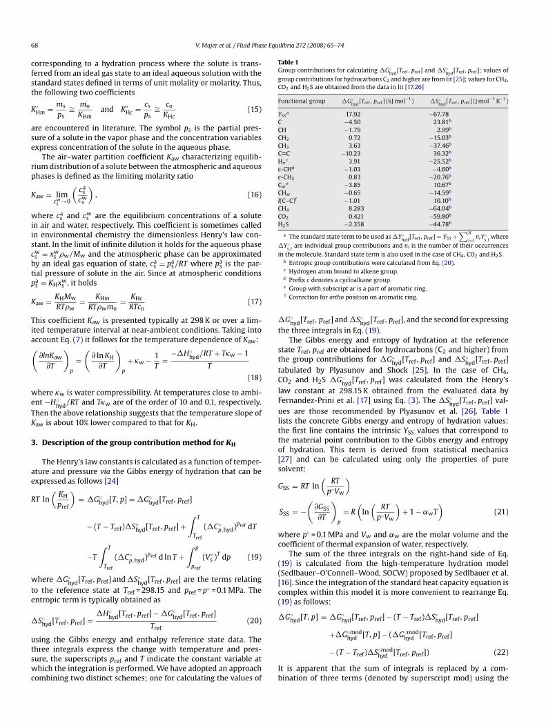
Table 1Group contributions for calculating �G◦

hyd[Tref, pref] and �S◦

hyd[Tref, pref]; values of

group contributions for hydrocarbons C2 and higher are from lit [25]; values for CH4,CO2 and H2S are obtained from the data in lit [17,26]

Functional group �G◦hyd

[Tref, pref] (kJ mol−1) �S◦hyd

[Tref, pref] (J mol−1 K−1)

YSSa 17.92 −67.78

C −4.50 23.81b

CH −1.79 2.99b

CH2 0.72 −15.03b

CH3 3.63 −37.46b

C C −10.23 36.32b

H�c 3.91 −25.52b

c-CHd −1.03 −4.60b

c-CH2 0.83 −20.76b

Care −3.85 10.67b

CHar −0.65 −14.59b

I(C–C)f −1.01 10.10b

CH4 8.283 −64.04b

CO2 0.421 −59.80b

H2S −2.358 −44.78b

a The standard state term to be used as �Y ◦hyd

[Tref, pref] = YSS +∑N

i=1niY ◦

s,iwhere

�Y ◦s,i

are individual group contributions and ni is the number of their occurrencesin the molecule. Standard state term is also used in the case of CH4, CO2 and H2S.

b Entropic group contributions were calculated from Eq. (20).c

�

t

sttClFultto[s

G

wc

(([c(

�

8 V. Majer et al. / Fluid Phas

orresponding to a hydration process where the solute is trans-erred from an ideal gas state to an ideal aqueous solution with thetandard states defined in terms of unit molality or molarity. Thus,he following two coefficients

′Hm = ms

ps∼= mo

KHmand K ′

Hc = cs

ps∼= co

KHc(15)

re encountered in literature. The symbol ps is the partial pres-ure of a solute in the vapor phase and the concentration variablesxpress concentration of the solute in the aqueous phase.

The air–water partition coefficient Kaw characterizing equilib-ium distribution of a solute between the atmospheric and aqueoushases is defined as the limiting molarity ratio

aw = limcw

s →0

(ca

scw

s

), (16)

here cas and cw

s are the equilibrium concentrations of a soluten air and water, respectively. This coefficient is sometimes calledn environmental chemistry the dimensionless Henry’s law con-tant. In the limit of infinite dilution it holds for the aqueous phasews = xw

s �w/Mw and the atmospheric phase can be approximatedy an ideal gas equation of state, ca

s = pas/RT where pa

s is the par-ial pressure of solute in the air. Since at atmospheric conditionsas = KHxw

s , it holds

aw = KHMw

RT�w= KHm

RT�wmo= KHc

RTco(17)

his coefficient Kaw is presented typically at 298 K or over a lim-ted temperature interval at near-ambient conditions. Taking intoccount Eq. (7) it follows for the temperature dependence of Kaw:

∂lnKaw

∂T

)p

=(

∂ ln KH

∂T

)p

+ �w − 1T

=−�H◦

hyd/RT + T�w − 1

T

(18)

here �w is water compressibility. At temperatures close to ambi-nt −H◦

hyd/RT and T�w are of the order of 10 and 0.1, respectively.hen the above relationship suggests that the temperature slope ofaw is about 10% lower compared to that for KH.

. Description of the group contribution method for KH

The Henry’s law constants is calculated as a function of temper-ture and pressure via the Gibbs energy of hydration that can bexpressed as follows [24]

T ln(

KH

pref

)= �G◦

hyd[T, p] = �G◦hyd[Tref, pref]

− (T − Tref)�S◦hyd[Tref, pref] +

∫ T

Tref

(�C◦p,hyd)pref dT

−T

∫ T

Tref

(�C◦p,hyd)pref d ln T +

∫ p

pref

(V ◦s )T dp (19)

here �G◦hyd[Tref, pref] and �S◦

hyd[Tref, pref] are the terms relatingo the reference state at Tref = 298.15 and pref = p◦ = 0.1 MPa. Thentropic term is typically obtained as

S◦hyd[Tref, pref] =

�H◦hyd[Tref, pref] − �G◦

hyd[Tref, pref]

Tref(20)

sing the Gibbs energy and enthalpy reference state data. Thehree integrals express the change with temperature and pres-ure, the superscripts pref and T indicate the constant variable athich the integration is performed. We have adopted an approach

ombining two distinct schemes; one for calculating the values ofIb

Hydrogen atom bound to alkene group.d Prefix c denotes a cycloalkane group.e Group with subscript ar is a part of aromatic ring.f Correction for ortho position on aromatic ring.

G◦hyd[Tref, pref] and �S◦

hyd[Tref, pref], and the second for expressinghe three integrals in Eq. (19).

The Gibbs energy and entropy of hydration at the referencetate Tref, pref are obtained for hydrocarbons (C2 and higher) fromhe group contributions for �G◦

hyd[Tref, pref] and �S◦hyd[Tref, pref]

abulated by Plyasunov and Shock [25]. In the case of CH4,O2 and H2S �G◦

hyd[Tref, pref] was calculated from the Henry’saw constant at 298.15 K obtained from the evaluated data byernandez-Prini et al. [17] using Eq. (3). The �S◦

hyd[Tref, pref] val-es are those recommended by Plyasunov et al. [26]. Table 1

ists the concrete Gibbs energy and entropy of hydration values:he first line contains the intrinsic YSS values that correspond tohe material point contribution to the Gibbs energy and entropyf hydration. This term is derived from statistical mechanics27] and can be calculated using only the properties of pureolvent:

SS = RT ln(

RT

p◦Vw

)

SSS = −(

∂GSS

∂T

)p

= R(

ln(

RT

p◦Vw

)+ 1 − ˛wT

)(21)

here p◦ = 0.1 MPa and Vw and ˛w are the molar volume and theoefficient of thermal expansion of water, respectively.

The sum of the three integrals on the right-hand side of Eq.19) is calculated from the high-temperature hydration modelSedlbauer–O’Connell–Wood, SOCW) proposed by Sedlbauer et al.16]. Since the integration of the standard heat capacity equation isomplex within this model it is more convenient to rearrange Eq.19) as follows:

G◦hyd[T, p] = �G◦

hyd[Tref, pref] − (T − Tref)�S◦hyd[Tref, pref]

+�G◦mod[T, p] − (�G◦mod[Tref, pref]

hyd hyd

− (T − Tref)�S◦modhyd [Tref, pref]) (22)

t is apparent that the sum of integrals is replaced by a com-ination of three terms (denoted by superscript mod) using the

V. Majer et al. / Fluid Phase Equilibria 272 (2008) 65–74 69

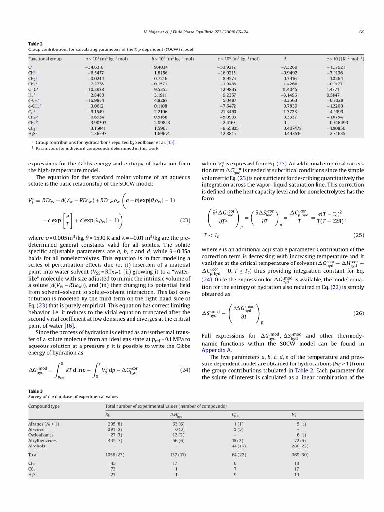
Table 2Group contributions for calculating parameters of the T, p dependent (SOCW) model

Functional group a × 103 (m3 kg−1 mol) b × 104 (m3 kg−1 mol) c × 106 (m3 kg−1 mol) d e × 10 (J K−2 mol−1)

Ca −34.6310 9.4034 −53.9212 −7.3260 −13.7921CHa −6.5437 1.8156 −16.9215 −0.9492 −3.9136CH2

a −0.0244 0.7216 −8.9576 0.3416 −1.8264CH3

a 7.2778 −0.1571 −1.9499 1.4268 −0.0177C Ca −10.2988 −9.5352 −12.9835 11.4045 1.4871H�

a 2.8400 3.1911 9.2357 −3.1496 0.5847c-CHa −16.9864 4.8289 5.0487 −3.3563 −0.9028c-CH2

a 3.0612 0.1108 −7.6472 0.7839 −1.2200Car

a −9.1549 2.2106 −21.3460 −1.3723 −4.9993CHar

a 0.6924 0.5168 −5.0903 0.3337 −1.0754CH4

b 3.90203 2.09843 −2.4163 0 −0.746493CO2

b 3.15041 1.5963 −9.65805 0.407478 −1.90856H

et

s

V

wdshsplaftEbsp

fae

�

wtviif

wcv�

(to

�

Fn

TS

C

AACAA

T

CCH

2Sb 1.36697 1.69674

a Group contributions for hydrocarbons reported by Sedlbauer et al. [15].b Parameters for individual compounds determined in this work.

xpressions for the Gibbs energy and entropy of hydration fromhe high-temperature model.

The equation for the standard molar volume of an aqueousolute is the basic relationship of the SOCW model:

◦s = RT�w + d(Vw − RT�w) + RT�w�w

(a + b(exp[ϑ�w] − 1)

+ c exp

[

T

]+ ı(exp[��w] − 1)

)(23)

here � = 0.005 m3/kg, = 1500 K and � = −0.01 m3/kg are the pre-etermined general constants valid for all solutes. The solutepecific adjustable parameters are a, b, c and d, while ı = 0.35aolds for all nonelectrolytes. This equation is in fact modeling aeries of perturbation effects due to: (i) insertion of a materialoint into water solvent (VSS = RT�w), (ii) growing it to a “water-

ike” molecule with size adjusted to mimic the intrinsic volume ofsolute (d(Vw − RT�w)), and (iii) then changing its potential field

rom solvent–solvent to solute–solvent interaction. This last con-ribution is modeled by the third term on the right-hand side ofq. (23) that is purely empirical. This equation has correct limitingehavior, i.e. it reduces to the virial equation truncated after theecond virial coefficient at low densities and diverges at the criticaloint of water [16].

Since the process of hydration is defined as an isothermal trans-er of a solute molecule from an ideal gas state at pref = 0.1 MPa toqueous solution at a pressure p it is possible to write the Gibbs

nergy of hydration as

G◦modhyd =

∫ 0

pref

RT d ln p +∫ p

0

V ◦s dp + �G◦cor

hyd (24)

A

stt

able 3urvey of the database of experimental values

ompound type Total number of experimental values (number of c

KH �H◦hyd

lkanes (NC > 1) 295 (8) 63 (6)lkenes 291 (5) 6 (3)ycloalkanes 27 (3) 12 (2)lkylbenzenes 445 (7) 56 (6)lcohols – –

otal 1058 (23) 137 (17)

H4 45 17O2 73 12S 27 1

−12.8815 0.443516 −2.81635

here V ◦s is expressed from Eq. (23). An additional empirical correc-

ion term �G◦corhyd is needed at subcritical conditions since the simple

olumetric Eq. (23) is not sufficient for describing quantitatively thentegration across the vapor–liquid saturation line. This corrections defined on the heat capacity level and for nonelectrolytes has theorm

−(

∂2�G◦corhyd

∂T2

)p

=(

∂�S◦corhyd

∂T

)p

=�C◦cor

p,hyd

T= e(T − Tc)2

T(T − 228),

T < Tc (25)

here e is an additional adjustable parameter. Contribution of theorrection term is decreasing with increasing temperature and itanishes at the critical temperature of solvent (�G◦cor

hyd = �H◦corhyd =

C◦corp,hyd = 0, T ≥ Tc) thus providing integration constant for Eq.

24). Once the expression for �G◦modhyd is available, the model equa-

ion for the entropy of hydration also required in Eq. (22) is simplybtained as

S◦modhyd =

(∂�G◦mod

hyd

∂T

)p

(26)

ull expressions for �G◦modhyd , �S◦mod

hyd and other thermody-amic functions within the SOCW model can be found in

ppendix A.

The five parameters a, b, c, d, e of the temperature and pres-ure dependent model are obtained for hydrocarbons (NC > 1) fromhe group contributions tabulated in Table 2. Each parameter forhe solute of interest is calculated as a linear combination of the

ompounds)

C◦p,s V ◦

s

1 (1) 5 (1)3 (3) –– 6 (1)

16 (2) 72 (6)44 (16) 286 (22)

64 (22) 369 (30)

6 187 179 19

7 e Equilibria 272 (2008) 65–74

a

a

wsaTgdr((tancbsdttm

hCtcieHmswePswcTttOCnTit

sdsmatd3itm

O

Table 4Survey of data sources to determine the parameters of the SOCW model

Literature sources in chronologicalorder

Prop. Npoints T (K) p (MPa)

CH4

Michels et al. [28] KH 4 323–423 satCulberson and McKetta [29] KH 6 298–444 satSultanov et al. [30] KH 5 423–633 satRettich et al. [31] KH 16 275–328 satCramer [32] KH 7 297–518 satCrovetto et al. [33] KH 7 334–554 satDec and Gill [34] H 1 298 0.1Dec and Gill [35] H 2 288–308 0.1Oloffson et al. [36] H 3 288–308 0.1Naghibi et al. [37] H 11 273–323 0.1Hnedkovsky and Wood [38] Cp 6 303–623 28Tiepel and Gubbins [39] V 1 298 0.1Moore et al. [41] V 1 298 0.1Hnedkovsky et al. [42] V 16 298–623 28–35

CO2

Wiebe and Gaddy [43] KH 3 323–373 satWiebe and Gaddy [44] KH 3 304–313 satMorrison and Billet [45] KH 19 286–347 satMalinin [46] KH 4 473–603 satEllis and Golding [47] KH 9 450–582 satTakenouchi and Kennedy [48] KH 9 423–623 satMurray and Riley [49] KH 8 274–308 satCramer [32] KH 3 306–405 satShagiakhmetov and Tarzimanov

[50]KH 2 323–373 sat

Müller et al. [51] KH 6 373–473 satNishswander et al. [52] KH 2 353–471 satCrovetto and Wood [53] KH 3 623–643 satBamberger et al. [54] KH 2 333–353 satBerg and Vanderzee [55] H 1 298 0.1Barbero et al. [56] Cp 1 298 0.1Hnedkovsky and Wood [38] Cp 6 304–623 28Moore et al. [41] V 1 298 0.1Hnedkovsky et al. [42] V 16 298–623 20–35

H2SSelleck et al. [57] KH 3 377–444 satLee and Mather [58] KH 11 283–453 satGillespie and Wilson [59] KH 3 422–533 satCarroll and Mather [60] KH 10 273–333 satCox et al. [61] H 1 298 0.1Barbero et al. [62] Cp 3 283–313 0.1Hnedkovsky and Wood [38] Cp 6 304–623 28

wrprmpahtttlmos

0 V. Majer et al. / Fluid Phas

ppropriate parameters of constituting groups, e.g.

=N∑

i=1

niai (27)

here N is the total number of structural groups present in the givenolute, ni is the number of occurrences of each specific group, andi stands for the a parameter of the ith group taken from Table 2.he molecular fragments are defined in an identical way as theroup contributions used for the calculation at the reference con-itions Tref, pref (Table 1), the proximity effect I(C–C) on aromaticing is not, however, considered. The material point contributionEq. (21)) that is temperature dependent appears explicitly in Eq.24) and therefore it is not listed in Table 2. The group contribu-ions for C2 and higher hydrocarbons were taken over from therticle by Sedlbauer et al. [15]. For illustration Table 3 gives theumber of data points and compounds that were considered perlass of hydrocarbons when determining the group contributionsy simultaneous correlation of the experimental Henry’s law con-tants and their derivative properties. A certain amount of data onerivative properties (�C◦

p,hyd, V ◦s ) for alcohols were also included

hat was helpful for increasing numerical stability of the group con-ribution determination for the less frequent functional groups (for

ore information see reference [15]).Using analogous simultaneous correlation procedure like for

ydrocarbons, the parameters were newly determined for CH4,O2 and H2S. These three aqueous solutes belong to experimen-ally well-studied systems with data available for most propertiesharacterizing hydration at elevated temperatures and extendingn the case of V ◦

s and �C◦p,hyd to supercritical conditions. When

stablishing the parameters of the SOCW model we have used theenry’s law constants along the saturation line of water deter-ined from the gas solubility data reported in a variety of literature

ources listed in Table 4. Major sources of derivative propertiesere the papers by Hnedkovsky and Wood [38] and by Hnedkovsky

t al. [42], reporting the standard heat capacities obtained by theicker-type flow calorimetry and the standard volumes from mea-urements by vibrating tube densimetry, respectively. These dataere included for the three gases up to 623 K and 35 MPa in the

ase of volumes and at one isobar (28 MPa) for the heat capacities.he enthalpies of hydration are available for CH4 at temperatureso 323 K, originating from the unique measurements carried out byhe groups of Gill et al. [34,35,37] and Wadsö and co-workers [36].nly one enthalpic data point at 298 K is, however, reported forO2 and H2S. The properties of the solutes in the ideal gas phase,eeded for converting C◦

p,s to �C◦p,hyd, were taken from the JANAF

hermochemical Tables [40]. Overall numbers of data points relat-ng to individual thermodynamic properties are presented for thehree gases in Table 3 and a detailed survey is given in Table 4.

The parameters of the SOCW model were obtained by theimultaneous correlation of the Henry’s law constants and theata on the three derivative properties using the weighted leastquares procedure with weights reflecting the expected experi-ental uncertainties. They were estimated at 2% for KH of CH4 and

t 3% for CO2 and H2S, based on the root-mean-square deviations ofhe data from the correlation of Fernandez-Prini et al. [17]. For theerivative properties the expected errors were set between 1% and% for �H◦

hyd and V ◦s , and between 3% and 5% for �C◦

p,hyd, accord-ng to the error estimates in the original data sources and the facthat the relative error increases with the temperature. The objective

inimized function O was defined as

=4∑

j=1

nj∑i=1

[Xmod,j

i− Xexp,j

i

Xji

]2

(28)

t

t6f

Barbero et al. [56] V 3 283–313 0.1Hnedkovsky et al. [42] V 16 304–623 20–35

here Xj and Xj stand for KH, �H◦hyd, �C◦

p,hyd, V ◦s and their errors,

espectively, and nj are the numbers of data points for the fourroperties. Explicit equations for the thermodynamic functionsesulting from the SOCW model (denoted with the upper indexod in Eqs. (24)–(26)) are presented in Appendix A. The adjustable

arameters of the SOCW model obtained for aqueous CH4, CO2nd H2S are summarized in Table 2 along with parameters for theydrocarbon functional groups evaluated earlier [15]. A quantita-ive comparison is made in Table 5 between the data calculated forhe three gases from the SOCW model and the values resulting fromhe other two recently published models valid along the saturationine of water [17,63]. It is apparent that the agreement among the

odels at psatw is quantitative for CH4 and CO2. Some differences are

bserved for H2S due to higher uncertainty in the Henry’s law con-tants that are not quite consistent at elevated temperatures withhe �C◦

p,hyd and V ◦s data.

Figs. 1–4 illustrate the changes in the Henry’s law constant withhe structure of the solute and with temperature and pressure up to23 K and 80 MPa for hydrocarbons having eight carbon atoms andor the three gases. First the results of the calculation for KH from

V. Majer et al. / Fluid Phase Equilibria 272 (2008) 65–74 71

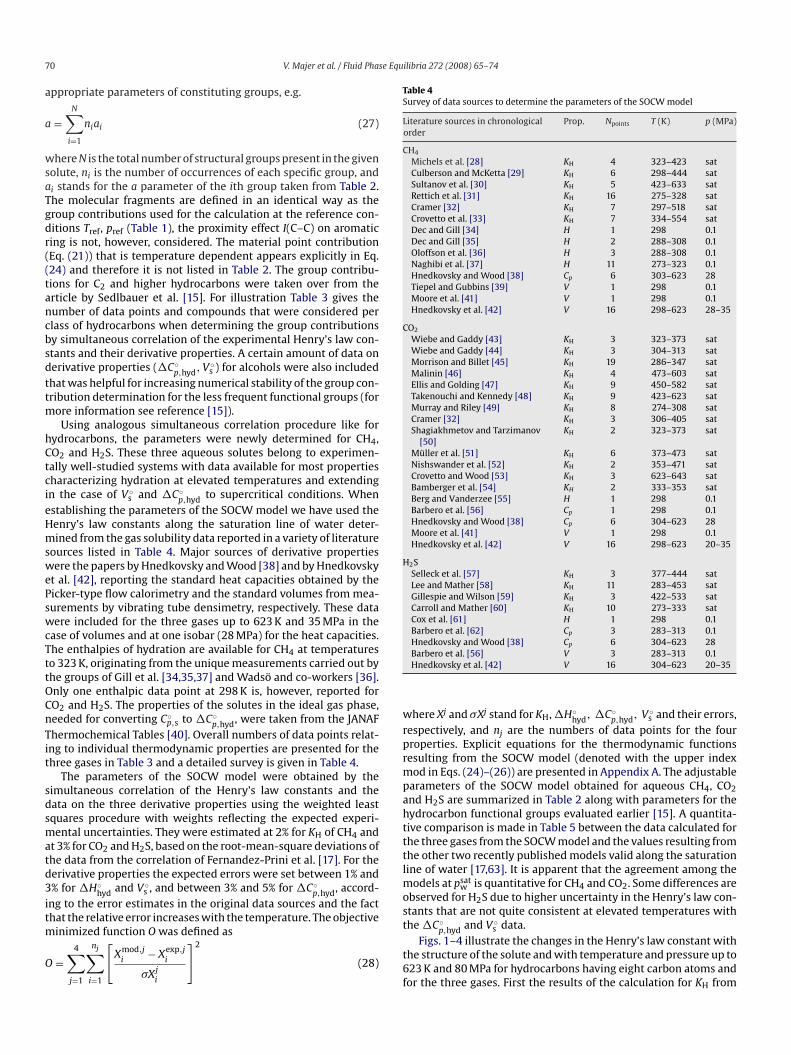
Fig. 1. The Henry’s law constants calculated along the saturation line of water fromthe group contribution model [15] for C8 hydrocarbons: n-octane (full), 1-octene(long-dashed), ethylcyclohexane (short-dashed) and ethylbenzene (dashed-dotline).

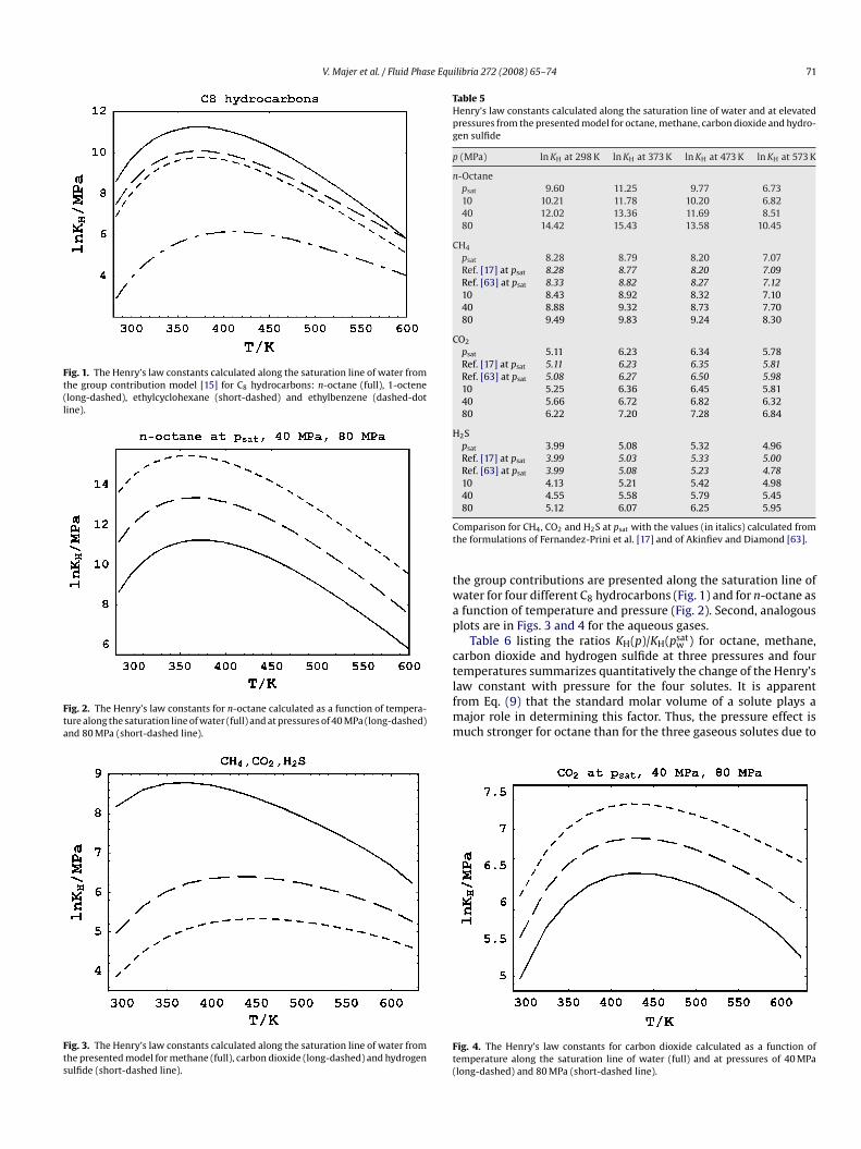
Fig. 2. The Henry’s law constants for n-octane calculated as a function of tempera-ture along the saturation line of water (full) and at pressures of 40 MPa (long-dashed)and 80 MPa (short-dashed line).

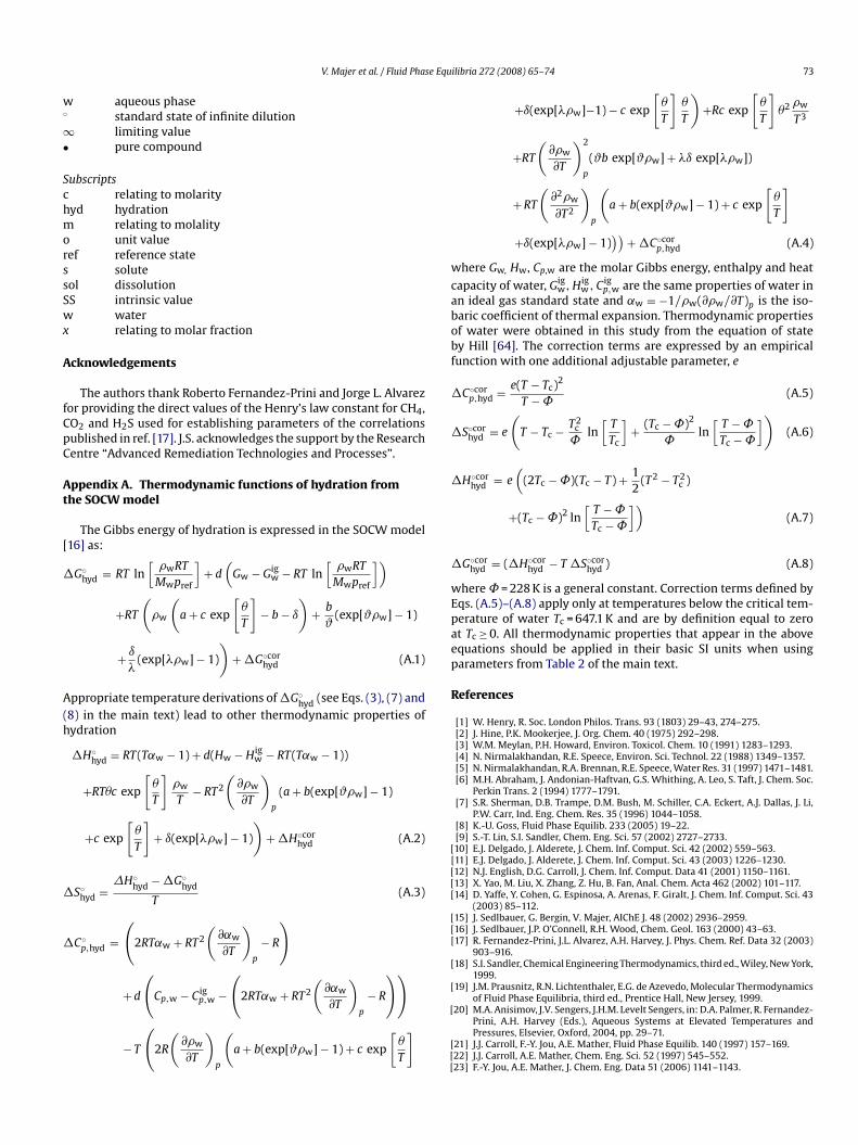
Fig. 3. The Henry’s law constants calculated along the saturation line of water fromthe presented model for methane (full), carbon dioxide (long-dashed) and hydrogensulfide (short-dashed line).

Table 5Henry’s law constants calculated along the saturation line of water and at elevatedpressures from the presented model for octane, methane, carbon dioxide and hydro-gen sulfide

p (MPa) ln KH at 298 K ln KH at 373 K ln KH at 473 K ln KH at 573 K

n-Octanepsat 9.60 11.25 9.77 6.7310 10.21 11.78 10.20 6.8240 12.02 13.36 11.69 8.5180 14.42 15.43 13.58 10.45

CH4

psat 8.28 8.79 8.20 7.07Ref. [17] at psat 8.28 8.77 8.20 7.09Ref. [63] at psat 8.33 8.82 8.27 7.1210 8.43 8.92 8.32 7.1040 8.88 9.32 8.73 7.7080 9.49 9.83 9.24 8.30

CO2

psat 5.11 6.23 6.34 5.78Ref. [17] at psat 5.11 6.23 6.35 5.81Ref. [63] at psat 5.08 6.27 6.50 5.9810 5.25 6.36 6.45 5.8140 5.66 6.72 6.82 6.3280 6.22 7.20 7.28 6.84

H2Spsat 3.99 5.08 5.32 4.96Ref. [17] at psat 3.99 5.03 5.33 5.00Ref. [63] at psat 3.99 5.08 5.23 4.7810 4.13 5.21 5.42 4.9840 4.55 5.58 5.79 5.45

Ct

twap

ctlfmm

Ft(

80 5.12 6.07 6.25 5.95

omparison for CH4, CO2 and H2S at psat with the values (in italics) calculated fromhe formulations of Fernandez-Prini et al. [17] and of Akinfiev and Diamond [63].

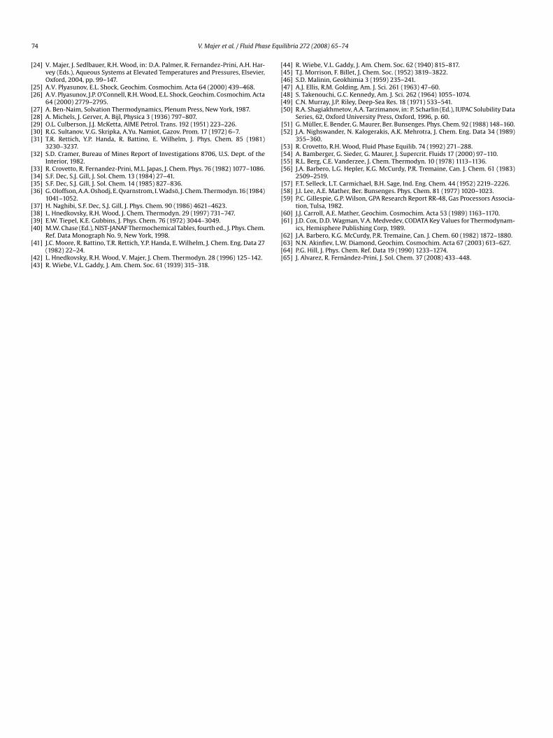
he group contributions are presented along the saturation line ofater for four different C8 hydrocarbons (Fig. 1) and for n-octane asfunction of temperature and pressure (Fig. 2). Second, analogouslots are in Figs. 3 and 4 for the aqueous gases.

Table 6 listing the ratios KH(p)/KH(psatw ) for octane, methane,

arbon dioxide and hydrogen sulfide at three pressures and fouremperatures summarizes quantitatively the change of the Henry’s

aw constant with pressure for the four solutes. It is apparentrom Eq. (9) that the standard molar volume of a solute plays a

ajor role in determining this factor. Thus, the pressure effect isuch stronger for octane than for the three gaseous solutes due to

ig. 4. The Henry’s law constants for carbon dioxide calculated as a function ofemperature along the saturation line of water (full) and at pressures of 40 MPalong-dashed) and 80 MPa (short-dashed line).

72 V. Majer et al. / Fluid Phase Equilibria 272 (2008) 65–74

Table 6Ratios KH(p)/KH(psat

w ) for octane, methane, carbon dioxide and hydrogen sulfide

KH(p)/KH(psatw ) 323 K (psat

w ≈ 0.1 MPa) 373 K (psatw ≈ 0.1 MPa) 473 K (psat

w ≈ 1.6 MPa) 573 K (psatw ≈ 8.7 MPa)

10 MPa 50 MPa 100 MPa 10 MPa 50 MPa 100 MPa 10 MPa 50 MPa 100 MPa 10 MPa 50 MPa 100 MPa

O 181C 3.6C 3.3H 3.4

tcewatKctp

4c

meeurtopHaorlacctaupntcimpccamdstf

K

wEs

ibic

cbfitt

LcCfGHKKKmMNOpRSSTVxXy

G˛�ϕ��

SaccegHi

ctane 1.8 17 289 1.7 14H4 1.2 2.0 4.0 1.1 1.9O2 1.1 1.9 3.7 1.1 1.82S 1.1 1.9 3.8 1.1 1.8

he difference in the V ◦s values (about 100 cm3/mol for C8H18 and

lose to 35 cm3/mol for the three gases at 298.15 K). At superambi-nt conditions, the standard molar volume increases substantiallyith increasing temperature and decreases with pressure, it scales

pproximately with the compressibility of water and diverges athe critical point of the solvent. For the pressures dependence ofH the increase in volume at high temperatures is, however, partlyompensated by dividing with temperature in Eq. (9). Therefore,he relative pressure effect on KH does not change much with tem-erature at conditions remote from the critical point of water.

. Software package for calculating the Henry’s lawonstant and related distribution coefficients

As apparent from the equations listed in Appendix A, the appliedodel is rather complex and requires the use of a fundamental

quation of state allowing calculation of the thermodynamic prop-rties of water. A programming effort would be necessary beforesing the method. In addition, the Henry’s law constant or anotherelated coefficients are required in varying pressure and concen-ration units depending on the users and erroneous conversionsften lead to confusion. For that reason we have prepared a com-uter code with a user-friendly interface allowing generation of theenry’s law constants from the model as a function of temperaturend pressure in several types of units as well as the calculation ofther two coefficients defined by Eqs. (13) and (16) that are closelyelated to the Henry’s law constant. Using the group contributionsisted in Tables 1 and 2 the estimations can be performed for normalnd branched alkanes and alkenes C2 to C12 and for the mono-yclic saturated or aromatic hydrocarbons (typically for C6 ringompounds) with one or several alkyl groups up to C8. In addition,he software uses specific parameters for methane, carbon dioxidend hydrogen sulfide. The calculations can be made at temperaturesp to 623 K either along the saturation line of water or at distinctairs of temperature and pressure (psat

w < p < 100 MPa). When run-ing the program the user chooses from several options allowinghe calculation of one of the following parameters: the Henry’s lawonstant KH defined in terms of the mol fraction (Eq. (1)), its mod-fications KHm and KHc (Eq. (6)) using as concentration variables

olality (mol/kg) or molarity (mol/m3), respectively, the air–waterartition coefficient Kaw (Eq. (16)) and the vapor–liquid distributiononstant (relative volatility) Kd (Eq. (13)). The air–water partitionoefficient is used for expressing the partition of a solute betweenir and water at near-ambient conditions and the calculation isade therefore only at pressures below 0.5 MPa. Similarly due to its

efinition the vapor–liquid distribution constant can be calculatedolely along the saturation line of water. The five coefficients are inhe code interconnected by the limiting conversion expressions asollows

KHm KHc�w KawRT�w Kd

H =

moMw=

coMw=

Mw=

psat,w(29)

here the meaning of individual symbols was explained above (seeqs. (6), (14) and (17)). Compared to Eq. (14) it is apparent that theaturation pressure of water is used in the conversion (Eq. (29))

lmRss

1.5 11 114 1.1 10 1011.1 1.9 3.6 1.0 2.2 4.51.1 1.8 3.2 1.0 2.0 3.61.1 1.8 3.2 1.0 1.9 3.4

nstead of fugacity. This simplifying assumption of an ideal gasehavior of the vapor phase can lead to an increase of uncertainty

n Kd at high temperatures where the fugacity coefficient of wateran differ significantly from unity.

The code is available on request as shareware for non-ommercial users from academia (contacts: vladimir.majer@univ-pclermont.fr and josef.sedlbauer@tul.cz). The preparation of inputles, the operation of the code and a few illustrative examples ofhe input and output files are described in the README documenthat is distributed along with the software.

ist of symbolsmolarityheat capacityfugacityGibbs energyenthalpy

aw air–water partition coefficientd vapor–liquid distribution coefficientH Henry’s law constant

molalitymolar masstotal number of functional groups in a moleculeminimized objective functionpressureuniversal gas constantentropy

S intrinsic valuethermodynamic temperaturevolumemolar fraction liquid phase

¯ partial molar property (X = G, H, S, V, C)molar fraction gaseous phase

reek lettersexpansivityactivity coefficient changefugacity coefficientcompressibilitydensityabsolute error

uperscriptsair phase

alc calculatedor correction termxp experimental

gas phaseproperty compatible with the Henry’s law

g ideal gas

liquid phase

od high-temperature modelproperty compatible with the Raoult’s law

at saturationol solubility

e Equ

w◦

∞•

SchmorssSwx

A

fCpC

At

[

�

A(h

�

�

w

cabobf

�

�

�

�

wEpaep

R

[[[[[

[[[

[

[

[20] M.A. Anisimov, J.V. Sengers, J.H.M. Levelt Sengers, in: D.A. Palmer, R. Fernandez-Prini, A.H. Harvey (Eds.), Aqueous Systems at Elevated Temperatures andPressures, Elsevier, Oxford, 2004, pp. 29–71.

V. Majer et al. / Fluid Phas

aqueous phasestandard state of infinite dilutionlimiting valuepure compound

ubscriptsrelating to molarity

yd hydrationrelating to molalityunit value

ef reference statesolute

ol dissolutionS intrinsic value

waterrelating to molar fraction

cknowledgements

The authors thank Roberto Fernandez-Prini and Jorge L. Alvarezor providing the direct values of the Henry’s law constant for CH4,O2 and H2S used for establishing parameters of the correlationsublished in ref. [17]. J.S. acknowledges the support by the Researchentre “Advanced Remediation Technologies and Processes”.

ppendix A. Thermodynamic functions of hydration fromhe SOCW model

The Gibbs energy of hydration is expressed in the SOCW model16] as:

G◦hyd = RT ln

[�wRT

Mwpref

]+ d(

Gw − Gigw − RT ln

[�wRT

Mwpref

])

+RT

(�w

(a + c exp

[

T

]− b − ı

)+ b

ϑ(exp[ϑ�w] − 1)

+ ı

�(exp[��w] − 1)

)+ �G◦cor

hyd (A.1)

ppropriate temperature derivations of �G◦hyd (see Eqs. (3), (7) and

8) in the main text) lead to other thermodynamic properties ofydration

�H◦hyd = RT(T˛w − 1) + d(Hw − Hig

w − RT(T˛w − 1))

+RTc exp

[

T

]�w

T− RT2

(∂�w

∂T

)p

(a + b(exp[ϑ�w] − 1)

+c exp

[

T

]+ ı(exp[��w] − 1)

)+ �H◦cor

hyd (A.2)

S◦hyd =

�H◦hyd − �G◦

hyd

T(A.3)

C◦p,hyd =

(2RT˛w + RT2

(∂˛w

∂T

)p

− R

)

+ d

(Cp,w − C ig

p,w −(

2RT˛w + RT2

(∂˛w

∂T

)p

− R

))( ( ) ( [ ]

− T 2R∂�w

∂Tp

a + b(exp[ϑ�w] − 1) + c exp

T[[[

ilibria 272 (2008) 65–74 73

+ı(exp[��w]−1) − c exp

[

T

]

T

)+Rc exp

[

T

]2 �w

T3

+RT

(∂�w

∂T

)2

p

(ϑb exp[ϑ�w] + �ı exp[��w])

+ RT

(∂2�w

∂T2

)p

(a + b(exp[ϑ�w] − 1) + c exp

[

T

]

+ı(exp[��w] − 1)))

+ �C◦corp,hyd (A.4)

here Gw, Hw, Cp,w are the molar Gibbs energy, enthalpy and heat

apacity of water, Gigw, Hig

w, C igp,w are the same properties of water in

n ideal gas standard state and ˛w = −1/�w(∂�w/∂T)p is the iso-aric coefficient of thermal expansion. Thermodynamic propertiesf water were obtained in this study from the equation of statey Hill [64]. The correction terms are expressed by an empiricalunction with one additional adjustable parameter, e

C◦corp,hyd = e(T − Tc)2

T − ˚(A.5)

S◦corhyd = e

(T − Tc − T2

c˚

ln[

T

Tc

]+ (Tc − ˚)2

˚ln[

T − ˚

Tc − ˚

])(A.6)

H◦corhyd = e

((2Tc − ˚)(Tc − T) + 1

2(T2 − T2

c )

+(Tc − ˚)2 ln[

T − ˚

Tc − ˚

])(A.7)

G◦corhyd = (�H◦cor

hyd − T �S◦corhyd ) (A.8)

here ˚ = 228 K is a general constant. Correction terms defined byqs. (A.5)–(A.8) apply only at temperatures below the critical tem-erature of water Tc = 647.1 K and are by definition equal to zerot Tc ≥ 0. All thermodynamic properties that appear in the abovequations should be applied in their basic SI units when usingarameters from Table 2 of the main text.

eferences

[1] W. Henry, R. Soc. London Philos. Trans. 93 (1803) 29–43, 274–275.[2] J. Hine, P.K. Mookerjee, J. Org. Chem. 40 (1975) 292–298.[3] W.M. Meylan, P.H. Howard, Environ. Toxicol. Chem. 10 (1991) 1283–1293.[4] N. Nirmalakhandan, R.E. Speece, Environ. Sci. Technol. 22 (1988) 1349–1357.[5] N. Nirmalakhandan, R.A. Brennan, R.E. Speece, Water Res. 31 (1997) 1471–1481.[6] M.H. Abraham, J. Andonian-Haftvan, G.S. Whithing, A. Leo, S. Taft, J. Chem. Soc.

Perkin Trans. 2 (1994) 1777–1791.[7] S.R. Sherman, D.B. Trampe, D.M. Bush, M. Schiller, C.A. Eckert, A.J. Dallas, J. Li,

P.W. Carr, Ind. Eng. Chem. Res. 35 (1996) 1044–1058.[8] K.-U. Goss, Fluid Phase Equilib. 233 (2005) 19–22.[9] S.-T. Lin, S.I. Sandler, Chem. Eng. Sci. 57 (2002) 2727–2733.10] E.J. Delgado, J. Alderete, J. Chem. Inf. Comput. Sci. 42 (2002) 559–563.11] E.J. Delgado, J. Alderete, J. Chem. Inf. Comput. Sci. 43 (2003) 1226–1230.12] N.J. English, D.G. Carroll, J. Chem. Inf. Comput. Data 41 (2001) 1150–1161.13] X. Yao, M. Liu, X. Zhang, Z. Hu, B. Fan, Anal. Chem. Acta 462 (2002) 101–117.14] D. Yaffe, Y. Cohen, G. Espinosa, A. Arenas, F. Giralt, J. Chem. Inf. Comput. Sci. 43

(2003) 85–112.15] J. Sedlbauer, G. Bergin, V. Majer, AIChE J. 48 (2002) 2936–2959.16] J. Sedlbauer, J.P. O’Connell, R.H. Wood, Chem. Geol. 163 (2000) 43–63.17] R. Fernandez-Prini, J.L. Alvarez, A.H. Harvey, J. Phys. Chem. Ref. Data 32 (2003)

903–916.18] S.I. Sandler, Chemical Engineering Thermodynamics, third ed., Wiley, New York,

1999.19] J.M. Prausnitz, R.N. Lichtenthaler, E.G. de Azevedo, Molecular Thermodynamics

of Fluid Phase Equilibria, third ed., Prentice Hall, New Jersey, 1999.

21] J.J. Carroll, F.-Y. Jou, A.E. Mather, Fluid Phase Equilib. 140 (1997) 157–169.22] J.J. Carroll, A.E. Mather, Chem. Eng. Sci. 52 (1997) 545–552.23] F.-Y. Jou, A.E. Mather, J. Chem. Eng. Data 51 (2006) 1141–1143.

7 e Equ

[

[[

[[[[[

[

[[[[

[[[[

[

[[

[[[[[[[

[[

[[[[

[[[

[[61] J.D. Cox, D.D. Wagman, V.A. Medvedev, CODATA Key Values for Thermodynam-

4 V. Majer et al. / Fluid Phas

24] V. Majer, J. Sedlbauer, R.H. Wood, in: D.A. Palmer, R. Fernandez-Prini, A.H. Har-vey (Eds.), Aqueous Systems at Elevated Temperatures and Pressures, Elsevier,Oxford, 2004, pp. 99–147.

25] A.V. Plyasunov, E.L. Shock, Geochim. Cosmochim. Acta 64 (2000) 439–468.26] A.V. Plyasunov, J.P. O’Connell, R.H. Wood, E.L. Shock, Geochim. Cosmochim. Acta

64 (2000) 2779–2795.27] A. Ben-Naim, Solvation Thermodynamics, Plenum Press, New York, 1987.28] A. Michels, J. Gerver, A. Bijl, Physica 3 (1936) 797–807.29] O.L. Culberson, J.J. McKetta, AIME Petrol. Trans. 192 (1951) 223–226.30] R.G. Sultanov, V.G. Skripka, A.Yu. Namiot, Gazov. Prom. 17 (1972) 6–7.31] T.R. Rettich, Y.P. Handa, R. Battino, E. Wilhelm, J. Phys. Chem. 85 (1981)

3230–3237.32] S.D. Cramer, Bureau of Mines Report of Investigations 8706, U.S. Dept. of the

Interior, 1982.33] R. Crovetto, R. Fernandez-Prini, M.L. Japas, J. Chem. Phys. 76 (1982) 1077–1086.34] S.F. Dec, S.J. Gill, J. Sol. Chem. 13 (1984) 27–41.35] S.F. Dec, S.J. Gill, J. Sol. Chem. 14 (1985) 827–836.36] G. Oloffson, A.A. Oshodj, E. Qvarnstrom, I. Wadsö, J. Chem. Thermodyn. 16 (1984)

1041–1052.37] H. Naghibi, S.F. Dec, S.J. Gill, J. Phys. Chem. 90 (1986) 4621–4623.38] L. Hnedkovsky, R.H. Wood, J. Chem. Thermodyn. 29 (1997) 731–747.39] E.W. Tiepel, K.E. Gubbins, J. Phys. Chem. 76 (1972) 3044–3049.

40] M.W. Chase (Ed.), NIST-JANAF Thermochemical Tables, fourth ed., J. Phys. Chem.

Ref. Data Monograph No. 9, New York, 1998.41] J.C. Moore, R. Battino, T.R. Rettich, Y.P. Handa, E. Wilhelm, J. Chem. Eng. Data 27

(1982) 22–24.42] L. Hnedkovsky, R.H. Wood, V. Majer, J. Chem. Thermodyn. 28 (1996) 125–142.43] R. Wiebe, V.L. Gaddy, J. Am. Chem. Soc. 61 (1939) 315–318.

[[[[

ilibria 272 (2008) 65–74

44] R. Wiebe, V.L. Gaddy, J. Am. Chem. Soc. 62 (1940) 815–817.45] T.J. Morrison, F. Billet, J. Chem. Soc. (1952) 3819–3822.46] S.D. Malinin, Geokhimia 3 (1959) 235–241.47] A.J. Ellis, R.M. Golding, Am. J. Sci. 261 (1963) 47–60.48] S. Takenouchi, G.C. Kennedy, Am. J. Sci. 262 (1964) 1055–1074.49] C.N. Murray, J.P. Riley, Deep-Sea Res. 18 (1971) 533–541.50] R.A. Shagiakhmetov, A.A. Tarzimanov, in: P. Scharlin (Ed.), IUPAC Solubility Data

Series, 62, Oxford University Press, Oxford, 1996, p. 60.51] G. Müller, E. Bender, G. Maurer, Ber. Bunsenges. Phys. Chem. 92 (1988) 148–160.52] J.A. Nighswander, N. Kalogerakis, A.K. Mehrotra, J. Chem. Eng. Data 34 (1989)

355–360.53] R. Crovetto, R.H. Wood, Fluid Phase Equilib. 74 (1992) 271–288.54] A. Bamberger, G. Sieder, G. Maurer, J. Supercrit. Fluids 17 (2000) 97–110.55] R.L. Berg, C.E. Vanderzee, J. Chem. Thermodyn. 10 (1978) 1113–1136.56] J.A. Barbero, L.G. Hepler, K.G. McCurdy, P.R. Tremaine, Can. J. Chem. 61 (1983)

2509–2519.57] F.T. Selleck, L.T. Carmichael, B.H. Sage, Ind. Eng. Chem. 44 (1952) 2219–2226.58] J.I. Lee, A.E. Mather, Ber. Bunsenges. Phys. Chem. 81 (1977) 1020–1023.59] P.C. Gillespie, G.P. Wilson, GPA Research Report RR-48, Gas Processors Associa-

tion, Tulsa, 1982.60] J.J. Carroll, A.E. Mather, Geochim. Cosmochim. Acta 53 (1989) 1163–1170.

ics, Hemisphere Publishing Corp, 1989.62] J.A. Barbero, K.G. McCurdy, P.R. Tremaine, Can. J. Chem. 60 (1982) 1872–1880.63] N.N. Akinfiev, L.W. Diamond, Geochim. Cosmochim. Acta 67 (2003) 613–627.64] P.G. Hill, J. Phys. Chem. Ref. Data 19 (1990) 1233–1274.65] J. Alvarez, R. Fernández-Prini, J. Sol. Chem. 37 (2008) 433–448.