Here is a plot of Integral(sin(x)). The data was generated byMathematica, with

Table[{x,N[SinIntegral[x]]},{x,0,20}]

and then copied to this document.

\psset{xunit=.2cm,yunit=1.5cm}

\savedata{\mydata}[

{{0, 0}, {1., 0.946083}, {2., 1.60541}, {3., 1.84865}, {4., 1.7582},

{5., 1.54993}, {6., 1.42469}, {7., 1.4546}, {8., 1.57419},

{9., 1.66504}, {10., 1.65835}, {11., 1.57831}, {12., 1.50497},

{13., 1.49936}, {14., 1.55621}, {15., 1.61819}, {16., 1.6313},

{17., 1.59014}, {18., 1.53661}, {19., 1.51863}, {20., 1.54824}}]

\dataplot[plotstyle=curve,showpoints=true,

dotstyle=triangle]{\mydata}

\psline{<->}(0,2)(0,0)(20,0)

\listplot*[par]{list}

\listplot is yet another way of plotting lists of data. This time,list should be a list of data (coordinate pairs), delimited only bywhite space. list is first expanded by TEX and then by PostScript.This means that list might be a PostScript program that leaveson the stack a list of data, but you can also include data thathas been retrieved with \readdata and \dataplot. However, whenusing the line, polygon or dots plotstyles with showpoints=false,linearc=0pt and no arrows, \dataplot is much less likely than\listplot to exceed PostScript’s memory or stack limits. In thepreceding example, these restrictions were not satisfied, and sothe example is equivalent to when \listplot is used:

...

\listplot[plotstyle=curve,showpoints=true,

dotstyle=triangle]{\mydata}

...

\psplot*[par]{xmin}{xmax}{function}

\psplot can be used to plot a function f (x), if you know a littlePostScript. function should be the PostScript code for calculat-ing f (x). Note that you must use x as the dependent variable.PostScript is not designed for scientific computation, but \psplotis good for graphing simple functions right from within TEX. E.g.,

\psplot[plotpoints=200]{0}{720}{x sin}

Plots 21

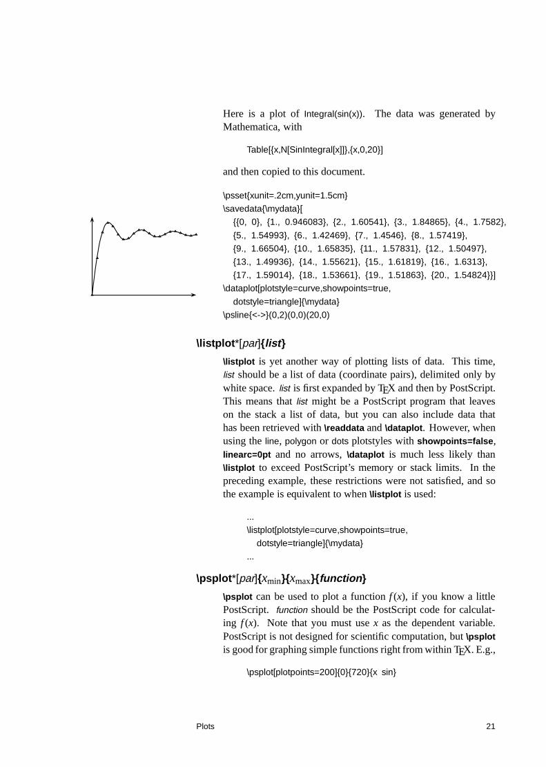
plots sin(x) from 0 to 720 degrees, by calculating sin(x) roughlyevery 3.6 degrees and then connecting the points with \psline.Here are plots of sin(x) cos((x=2)2) and sin2(x):

\psset{xunit=1.2pt}

\psplot[linecolor=gray,linewidth=1.5pt,plotstyle=curve]%

{0}{90}{x sin dup mul}

\psplot[plotpoints=100]{0}{90}{x sin x 2 div 2 exp cos mul}

\psline{<->}(0,-1)(0,1)

\psline{->}(100,0)

\parametricplot*[par]{tmin}{tmax}{function}

This is for a parametric plot of (x(t); y(t)). function is the PostScriptcode for calculating the pair x(t) y(t).

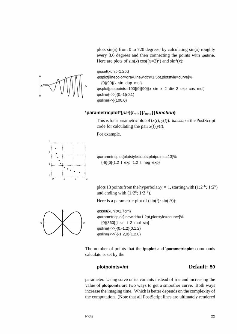
For example,

0 1 2 30

1

2

3

\parametricplot[plotstyle=dots,plotpoints=13]%

{-6}{6}{1.2 t exp 1.2 t neg exp}

plots 13 points from the hyperbola xy = 1, starting with (1:2–6; 1:26)and ending with (1:26; 1:2–6).

Here is a parametric plot of (sin(t); sin(2t)):

\psset{xunit=1.7cm}

\parametricplot[linewidth=1.2pt,plotstyle=ccurve]%

{0}{360}{t sin t 2 mul sin}

\psline{<->}(0,-1.2)(0,1.2)

\psline{<->}(-1.2,0)(1.2,0)

The number of points that the \psplot and \parametricplot commandscalculate is set by the

plotpoints=int Default: 50

parameter. Using curve or its variants instead of line and increasing thevalue of plotpoints are two ways to get a smoother curve. Both waysincrease the imaging time. Which is better depends on the complexity ofthe computation. (Note that all PostScript lines are ultimately rendered

Plots 22

as a series (perhaps short) line segments.) Mathematica generally useslineto to connect the points in its plots. The default minimum number ofplot points for Mathematica is 25, but unlike \psplot and \parametricplot,Mathematica increases the sampling frequency on sections of the curvewith greater fluctuation.

Plots 23

III More graphics parameters

The graphics parameters described in this part are common to all ormost of the graphics objects.

12 Coordinate systems

The following manipulations of the coordinate system apply only topure graphics objects.

A simple way to move the origin of the coordinate system to (x,y) iswith the

origin={coor} Default: 0pt,0pt

This is the one time that coordinates must be enclosed in curly brackets{} rather than parentheses ().

A simple way to switch swap the axes is with the

swapaxes=true Default: false

parameter. E.g., you might change your mind on the orientation of aplot after generating the data.

13 Line styles

The following graphics parameters (in addition to linewidth and line-color) determine how the lines are drawn, whether they be open orclosed curves.

linestyle=style Default: solid

Valid styles are none, solid, dashed and dotted.

More graphics parameters 24

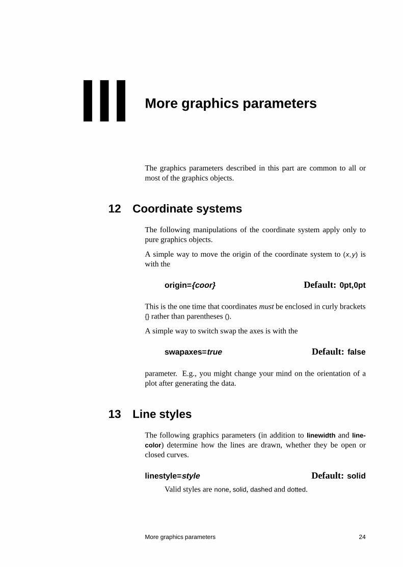
dash=dim1 dim2 Default: 5pt 3pt

The black-white dash pattern for the dashed line style. Forexample:

\psellipse[linestyle=dashed,dash=3pt 2pt](2,1)(2,1)

dotsep=dim Default: 3pt

The distance between dots in the dotted line style. For example

\psline[linestyle=dotted,dotsep=2pt]{|->>}(4,1)

border=dim Default: 0pt

A positive value draws a border of width dim and colorbordercolor on each side of the curve. This is useful for givingthe impression that one line passes on top of another. The valueis saved in the dimension register \psborder.

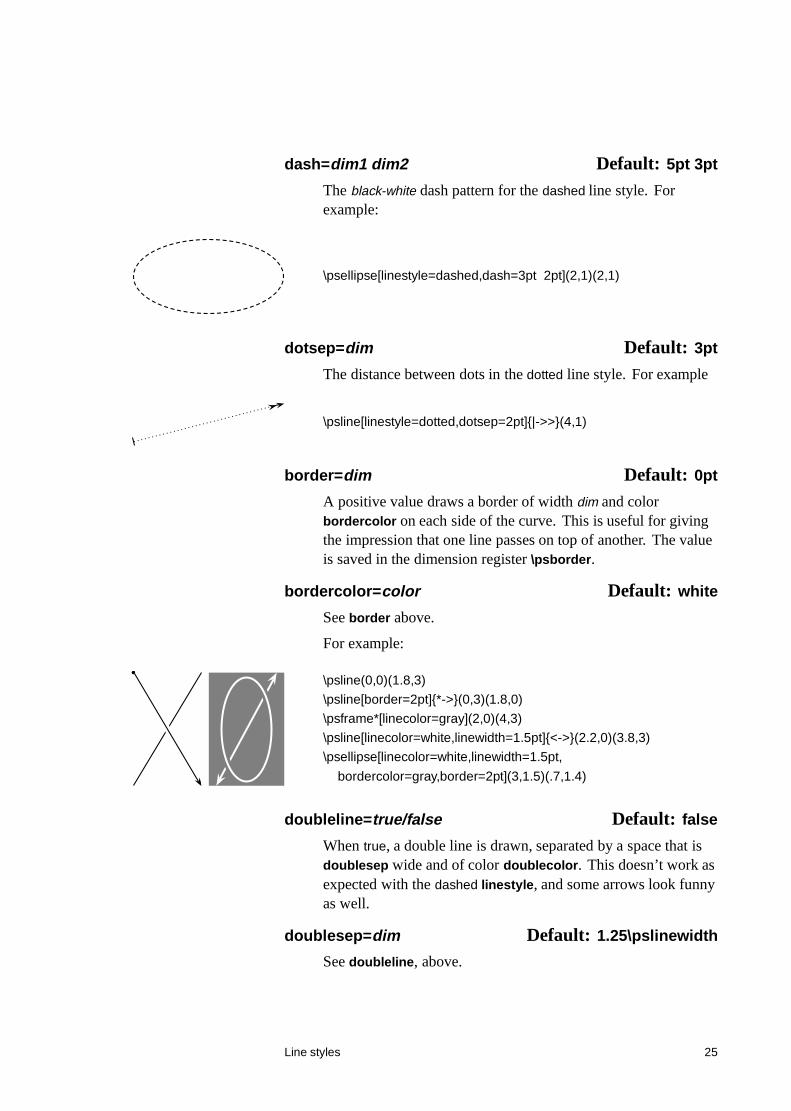
bordercolor=color Default: white

See border above.

For example:

\psline(0,0)(1.8,3)

\psline[border=2pt]{*->}(0,3)(1.8,0)

\psframe*[linecolor=gray](2,0)(4,3)

\psline[linecolor=white,linewidth=1.5pt]{<->}(2.2,0)(3.8,3)

\psellipse[linecolor=white,linewidth=1.5pt,

bordercolor=gray,border=2pt](3,1.5)(.7,1.4)

doubleline=true/false Default: false

When true, a double line is drawn, separated by a space that isdoublesep wide and of color doublecolor. This doesn’t work asexpected with the dashed linestyle, and some arrows look funnyas well.

doublesep=dim Default: 1.25\pslinewidth

See doubleline, above.

Line styles 25

doublecolor=color Default: white

See doubleline, above.

Here is an example of double lines:

\psline[doubleline=true,linearc=.5,

doublesep=1.5pt]{->}(0,0)(3,1)(4,0)

shadow=true/false Default: false

When true, a shadow is drawn, at a distance shadowsize fromthe original curve, in the direction shadowangle, and of colorshadowcolor.

shadowsize=dim Default: 3pt

See shadow, above.

shadowangle=angle Default: -45

See shadow, above.

shadowcolor=color Default: darkgray

See shadow, above.

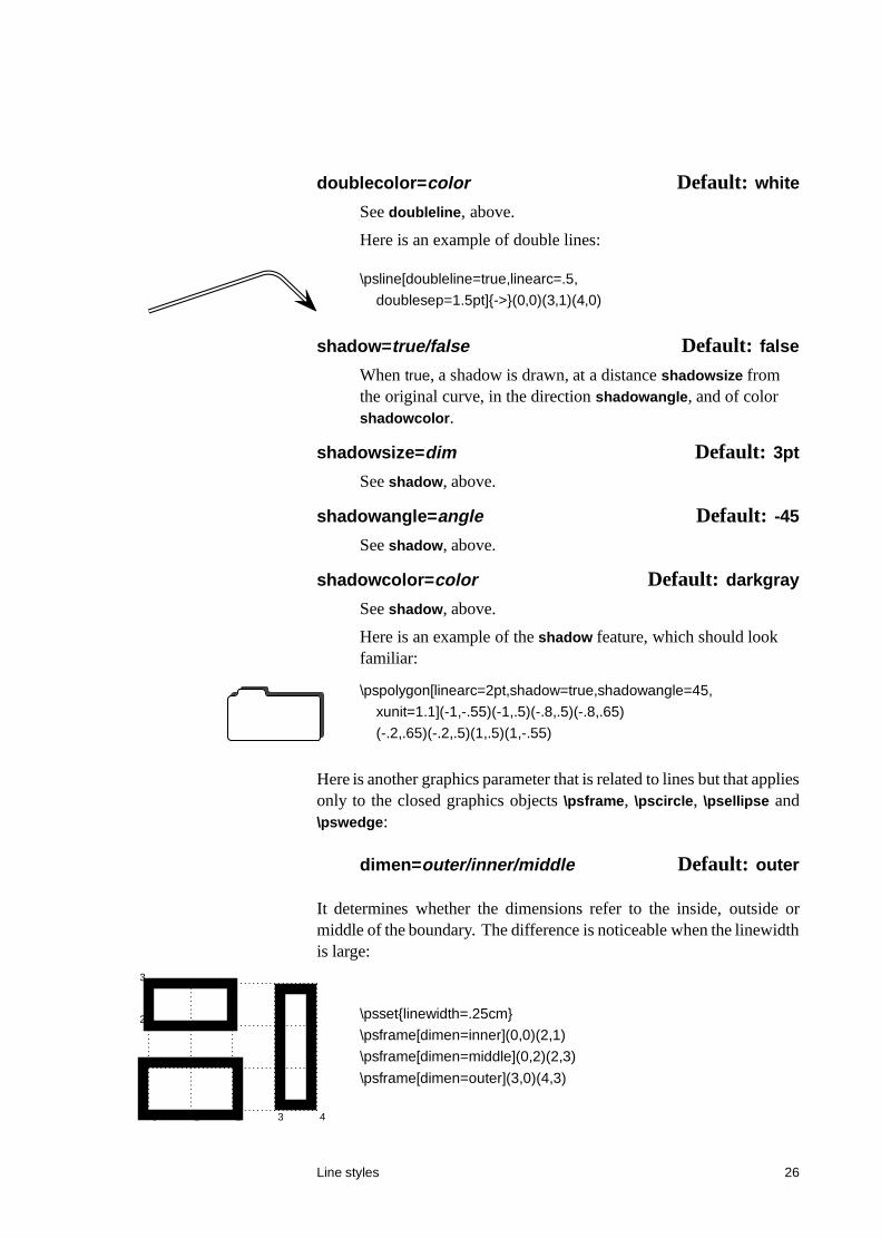
Here is an example of the shadow feature, which should lookfamiliar:

\pspolygon[linearc=2pt,shadow=true,shadowangle=45,

xunit=1.1](-1,-.55)(-1,.5)(-.8,.5)(-.8,.65)

(-.2,.65)(-.2,.5)(1,.5)(1,-.55)

Here is another graphics parameter that is related to lines but that appliesonly to the closed graphics objects \psframe, \pscircle, \psellipse and\pswedge:

dimen=outer/inner/middle Default: outer

It determines whether the dimensions refer to the inside, outside ormiddle of the boundary. The difference is noticeable when the linewidthis large:

0 1 2 3 40

1

2

3

\psset{linewidth=.25cm}

\psframe[dimen=inner](0,0)(2,1)

\psframe[dimen=middle](0,2)(2,3)

\psframe[dimen=outer](3,0)(4,3)

Line styles 26

With \pswedge, this only affects the radius; the origin always lies in themiddle the boundary. The right setting of this parameter depends onhow you want to align other objects.

14 Fill styles

The next group of graphics parameters determine how closed regionsare filled. Even open curves can be filled; this does not affect how thecurve is painted.

fillstyle=style Default: none

Valid styles are

none, solid, vlines, vlines*, hlines, hlines*, crosshatch

and crosshatch*.

vlines, hlines and crosshatch draw a pattern of lines, according tothe four parameters list below that are prefixed with hatch. The *

versions also fill the background, as in the solid style.

fillcolor=color Default: white

The background color in the solid, vlines*, hlines* and crosshatch*

styles.

hatchwidth=dim Default: .8pt

Width of lines.

hatchsep=dim Default: 4pt

Width of space between the lines.

hatchcolor=color Default: black

Color of lines. Saved in \pshatchcolor.

hatchangle=rot Default: 45

Rotation of the lines, in degrees. For example, if hatchangle isset to 45, the vlines style draws lines that run NW-SE, and thehlines style draws lines that run SW-NE, and the crosshatch styledraws both.

Here is an example of the vlines and related fill styles:

Fill styles 27

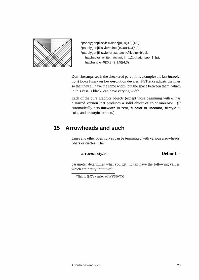
\pspolygon[fillstyle=vlines](0,0)(0,3)(4,0)

\pspolygon[fillstyle=hlines](0,0)(4,3)(4,0)

\pspolygon[fillstyle=crosshatch*,fillcolor=black,

hatchcolor=white,hatchwidth=1.2pt,hatchsep=1.8pt,

hatchangle=0](0,3)(2,1.5)(4,3)

Don’t be surprised if the checkered part of this example (the last \pspoly-gon) looks funny on low-resolution devices. PSTricks adjusts the linesso that they all have the same width, but the space between them, whichin this case is black, can have varying width.

Each of the pure graphics objects (except those beginning with q) hasa starred version that produces a solid object of color linecolor. (Itautomatically sets linewidth to zero, fillcolor to linecolor, fillstyle tosolid, and linestyle to none.)

15 Arrowheads and such

Lines and other open curves can be terminated with various arrowheads,t-bars or circles. The

arrows=style Default: -

parameter determines what you get. It can have the following values,which are pretty intuitive:5

5This is TEX’s version of WYSIWYG.

Arrowheads and such 28

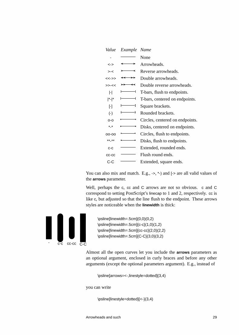
Value Example Name

- None

<-> Arrowheads.

>-< Reverse arrowheads.

<<->> Double arrowheads.

>>-<< Double reverse arrowheads.

|-| T-bars, flush to endpoints.

|*-|* T-bars, centered on endpoints.

[-] Square brackets.

(-) Rounded brackets.

o-o Circles, centered on endpoints.

*-* Disks, centered on endpoints.

oo-oo Circles, flush to endpoints.

**-** Disks, flush to endpoints.

c-c Extended, rounded ends.

cc-cc Flush round ends.

C-C Extended, square ends.

You can also mix and match. E.g., ->, *-) and [-> are all valid values ofthe arrows parameter.

Well, perhaps the c, cc and C arrows are not so obvious. c and C

correspond to setting PostScript’s linecap to 1 and 2, respectively. cc islike c, but adjusted so that the line flush to the endpoint. These arrowsstyles are noticeable when the linewidth is thick:

- c-c cc-cc C-C

\psline[linewidth=.5cm](0,0)(0,2)

\psline[linewidth=.5cm]{c-c}(1,0)(1,2)

\psline[linewidth=.5cm]{cc-cc}(2,0)(2,2)

\psline[linewidth=.5cm]{C-C}(3,0)(3,2)

Almost all the open curves let you include the arrows parameters asan optional argument, enclosed in curly braces and before any otherarguments (except the optional parameters argument). E.g., instead of

\psline[arrows=<-,linestyle=dotted](3,4)

you can write

\psline[linestyle=dotted]{<-}(3,4)

Arrowheads and such 29

The exceptions are a few streamlined macros that do not support the useof arrows (these all begin with q).

The size of these line terminators is controlled by the following parame-ters. In the description of the parameters, the width always refers to thedimension perpendicular to the line, and length refers to a dimension inthe direction of the line.

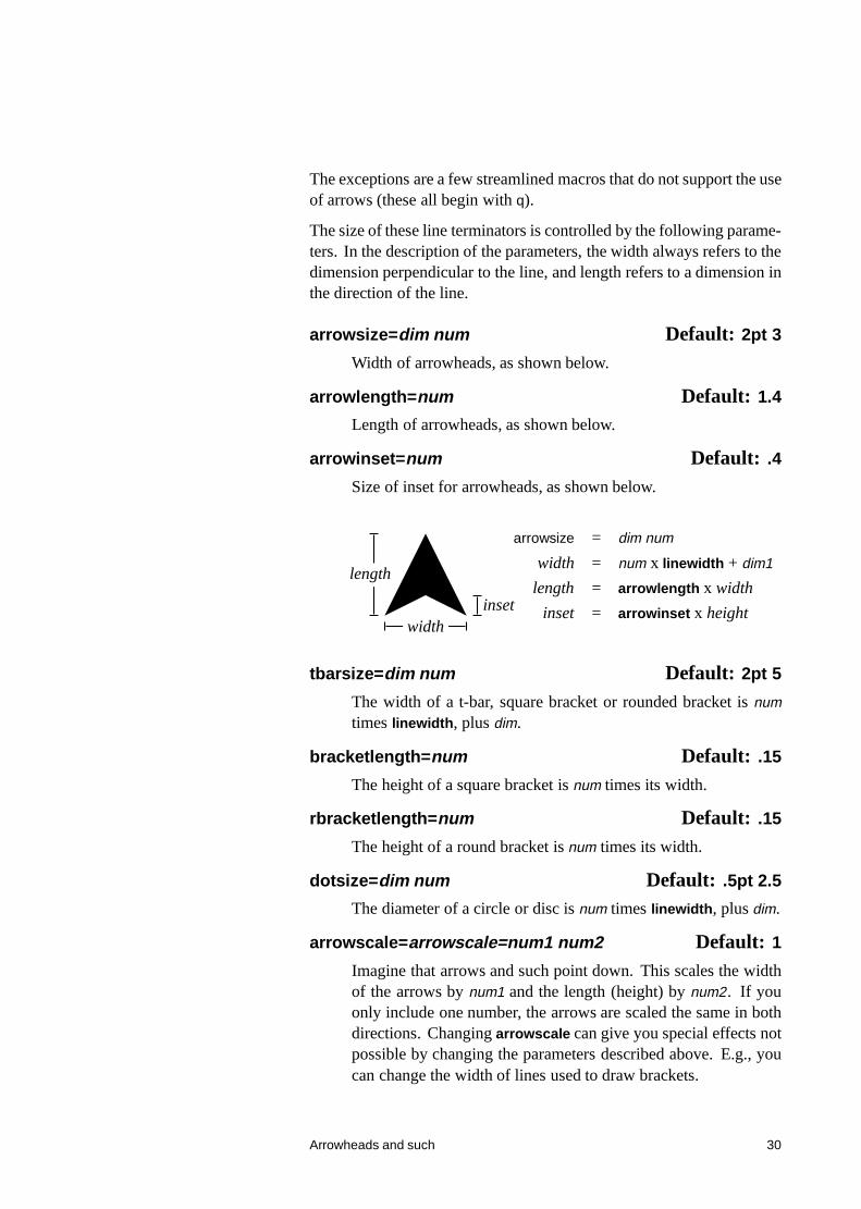
arrowsize=dim num Default: 2pt 3

Width of arrowheads, as shown below.

arrowlength=num Default: 1.4

Length of arrowheads, as shown below.

arrowinset=num Default: .4

Size of inset for arrowheads, as shown below.

length

widthinset

arrowsize = dim num

width = num x linewidth + dim1

length = arrowlength x width

inset = arrowinset x height

tbarsize=dim num Default: 2pt 5

The width of a t-bar, square bracket or rounded bracket is numtimes linewidth, plus dim.

bracketlength=num Default: .15

The height of a square bracket is num times its width.

rbracketlength=num Default: .15

The height of a round bracket is num times its width.

dotsize=dim num Default: .5pt 2.5

The diameter of a circle or disc is num times linewidth, plus dim.

arrowscale=arrowscale=num1 num2 Default: 1

Imagine that arrows and such point down. This scales the widthof the arrows by num1 and the length (height) by num2. If youonly include one number, the arrows are scaled the same in bothdirections. Changing arrowscale can give you special effects notpossible by changing the parameters described above. E.g., youcan change the width of lines used to draw brackets.

Arrowheads and such 30

16 Custom styles

You can define customized versions of any macro that has parameterchanges as an optional first argument using the \newpsobject command:

\newpsobject{name}{object}{par1=value1,…}

as in

\newpsobject{myline}{psline}{linecolor=green,linestyle=dotted}

\newpsobject{\mygrid}{psgrid}{subgriddiv=1,griddots=10,

gridlabels=7pt}

The first argument is the name of the new command you want to define.The second argument is the name of the graphics object. Note that bothof these arguments are given without the backslash. The third argumentis the special parameter values that you want to set.

With the above examples, the commands \myline and \mygrid work justlike the graphics object \psline it is based on, and you can even reset theparameters that you set when defining \myline, as in:

\myline[linecolor=gray,dotsep=2pt](5,6)

Another way to define custom graphics parameter configurations is withthe

\newpsstyle{name}{par1=value1,…}

command. You can then set the style graphics parameter to name, ratherthan setting the parameters given in the second argument of \newpsstyle.For example,

\newpsstyle{mystyle}{linecolor=green,linestyle=dotted}

\psline[style=mystyle](5,6)

Custom styles 31

IV Custom graphics

17 The basics

PSTricks contains a large palette of graphics objects, but sometimesyou need something special. For example, you might want to shade theregion between two curves. The

\pscustom*[par]{commands}

command lets you “roll you own” graphics object.

Let’s review how PostScript handles graphics. A path is a line, inthe mathematical sense rather than the visual sense. A path can haveseveral disconnected segments, and it can be open or closed. PostScripthas various operators for making paths. The end of the path is calledthe current point, but if there is no path then there is no current point.To turn the path into something visual, PostScript can fill the regionenclosed by the path (that is what fillstyle and such are about), andstroke the path (that is what linestyle and such are about).

At the beginning of \pscustom, there is no path. There are variouscommands that you can use in \pscustom for drawing paths. Someof these (the open curves) can also draw arrows. \pscustom fills andstrokes the path at the end, and for special effects, you can fill and strokethe path along the way using \psfill and \pstroke (see below).

Driver notes: \pscustom uses \pstverb and \pstunit. There are system-dependent limits on how long the argument of \special can be. You may runinto this limit using \pscustom because all the PostScript code accumulated by\pscustom is the argument of a single \special command.

18 Parameters

You need to keep the separation between drawing, stroking and fillingpaths in mind when setting graphics parameters. The linewidth andlinecolor parameters affect the drawing of arrows, but since the path

Custom graphics 32

commands do not stroke or fill the paths, these parameters, and thelinestyle, fillstyle and related parameters, do not have any other effect(except that in some cases linewidth is used in some calculations whendrawing the path). \pscustom and \fill make use of fillstyle and re-lated parameters, and \pscustom and \stroke make use of plinestyle andrelated parameters.

For example, if you include

\psline[linewidth=2pt,linecolor=blue,fillstyle=vlines]{<-}(3,3)(4,0)

in \pscustom, then the changes to linewidth and linecolor will affect thesize and color of the arrow but not of the line when it is stroked, and thechange to fillstyle will have no effect at all.

The shadow, border, doubleline and showpoints parameters are dis-abled in \pscustom, and the origin and swapaxes parameters only affect\pscustom itself, but there are commands (described below) that let youachieve these special effects.

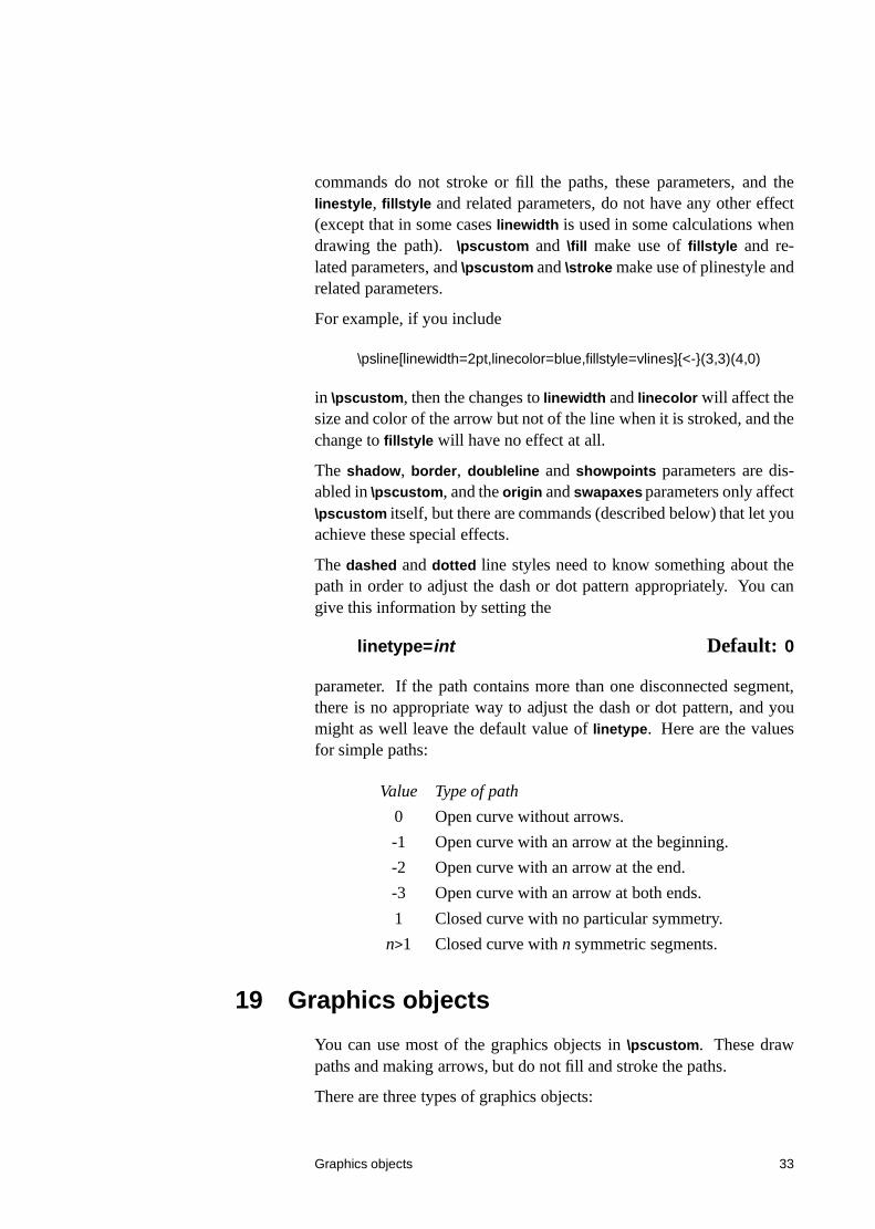
The dashed and dotted line styles need to know something about thepath in order to adjust the dash or dot pattern appropriately. You cangive this information by setting the

linetype=int Default: 0

parameter. If the path contains more than one disconnected segment,there is no appropriate way to adjust the dash or dot pattern, and youmight as well leave the default value of linetype. Here are the valuesfor simple paths:

Value Type of path

0 Open curve without arrows.

-1 Open curve with an arrow at the beginning.

-2 Open curve with an arrow at the end.

-3 Open curve with an arrow at both ends.

1 Closed curve with no particular symmetry.

n>1 Closed curve with n symmetric segments.

19 Graphics objects

You can use most of the graphics objects in \pscustom. These drawpaths and making arrows, but do not fill and stroke the paths.

There are three types of graphics objects:

Graphics objects 33

Special Special graphics objects include \psgrid, \psdots, \qline and\qdisk. You cannot use special graphics objects in \pscustom.

Closed You are allowed to use closed graphics objects in \pscustom,but their effect is unpredictable.6 Usually you would use the opencurves plus \closepath (see below) to draw closed curves.

Open The open graphics objects are the most useful commands fordrawing paths with \pscustom. By piecing together several opencurves, you can draw arbitrary paths. The rest of this sectionpertains to the open graphics objects.

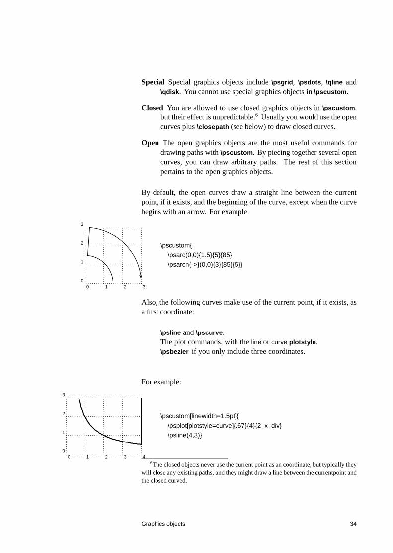
By default, the open curves draw a straight line between the currentpoint, if it exists, and the beginning of the curve, except when the curvebegins with an arrow. For example

0 1 2 30

1

2

3

\pscustom{

\psarc(0,0){1.5}{5}{85}

\psarcn{->}(0,0){3}{85}{5}}

Also, the following curves make use of the current point, if it exists, asa first coordinate:

\psline and \pscurve.The plot commands, with the line or curve plotstyle.\psbezier if you only include three coordinates.

For example:

0 1 2 3 40

1

2

3

\pscustom[linewidth=1.5pt]{

\psplot[plotstyle=curve]{.67}{4}{2 x div}

\psline(4,3)}

6The closed objects never use the current point as an coordinate, but typically theywill close any existing paths, and they might draw a line between the currentpoint andthe closed curved.

Graphics objects 34

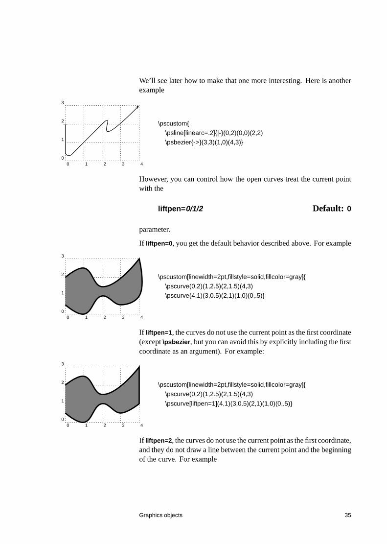
We’ll see later how to make that one more interesting. Here is anotherexample

0 1 2 3 40

1

2

3

\pscustom{

\psline[linearc=.2]{|-}(0,2)(0,0)(2,2)

\psbezier{->}(3,3)(1,0)(4,3)}

However, you can control how the open curves treat the current pointwith the

liftpen=0/1/2 Default: 0

parameter.

If liftpen=0, you get the default behavior described above. For example

0 1 2 3 40

1

2

3

\pscustom[linewidth=2pt,fillstyle=solid,fillcolor=gray]{

\pscurve(0,2)(1,2.5)(2,1.5)(4,3)

\pscurve(4,1)(3,0.5)(2,1)(1,0)(0,.5)}

If liftpen=1, the curves do not use the current point as the first coordinate(except \psbezier, but you can avoid this by explicitly including the firstcoordinate as an argument). For example:

0 1 2 3 40

1

2

3

\pscustom[linewidth=2pt,fillstyle=solid,fillcolor=gray]{

\pscurve(0,2)(1,2.5)(2,1.5)(4,3)

\pscurve[liftpen=1](4,1)(3,0.5)(2,1)(1,0)(0,.5)}

If liftpen=2, the curves do not use the current point as the first coordinate,and they do not draw a line between the current point and the beginningof the curve. For example

Graphics objects 35

0 1 2 3 40

1

2

3

\pscustom[linewidth=2pt,fillstyle=solid,fillcolor=gray]{

\pscurve(0,2)(1,2.5)(2,1.5)(4,3)

\pscurve[liftpen=2](4,1)(3,0.5)(2,1)(1,0)(0,.5)}

Later we will use the second example to fill the region between the twocurves, and then draw the curves.

20 Safe tricks

The commands described under this heading, which can only be usedin \pscustom, do not run a risk of PostScript errors (assuming yourdocument compiles without TEX errors).

Let’s start with some path, fill and stroke commands:

\newpath

Clear the path and the current point.

\moveto(coor)

This moves the current point to (x,y).

\closepath

This closes the path, joining the beginning and end of each piece(there may be more than one piece if you use \moveto).7

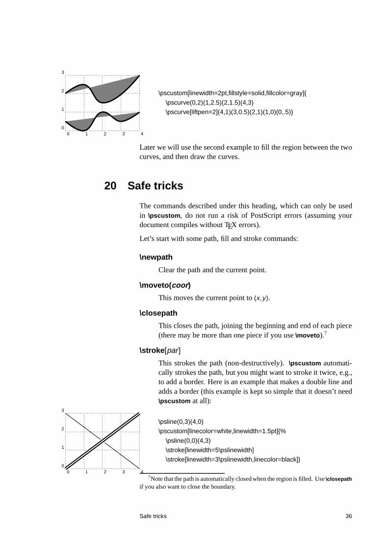
\stroke[par]

This strokes the path (non-destructively). \pscustom automati-cally strokes the path, but you might want to stroke it twice, e.g.,to add a border. Here is an example that makes a double line andadds a border (this example is kept so simple that it doesn’t need\pscustom at all):

0 1 2 3 40

1

2

3

\psline(0,3)(4,0)

\pscustom[linecolor=white,linewidth=1.5pt]{%

\psline(0,0)(4,3)

\stroke[linewidth=5\pslinewidth]

\stroke[linewidth=3\pslinewidth,linecolor=black]}

7Note that the path is automatically closed when the region is filled. Use \closepathif you also want to close the boundary.

Safe tricks 36

\fill[par]

This fills the region (non-destructively). \pscustom automaticallyfills the region as well.

\gsave

This saves the current graphics state (i.e., the path, color, linewidth, coordinate system, etc.) \grestore restores the graphicsstate. \gsave and \grestore must be used in pairs, properly nestedwith respect to TEX groups. You can have have nested \gsave-\grestore pairs.

\grestore

See above.

Here is an example that fixes an earlier example, using \gsaveand \grestore:

\psline{<->}(0,3)(0,0)(4,0)

\pscustom[linewidth=1.5pt]{

\psplot[plotstyle=curve]{.67}{4}{2 x div}

\gsave

\psline(4,3)

\fill[fillstyle=solid,fillcolor=gray]

\grestore}

Observe how the line added by \psline(4,3) is never stroked, be-cause it is nested in \gsave and \grestore.

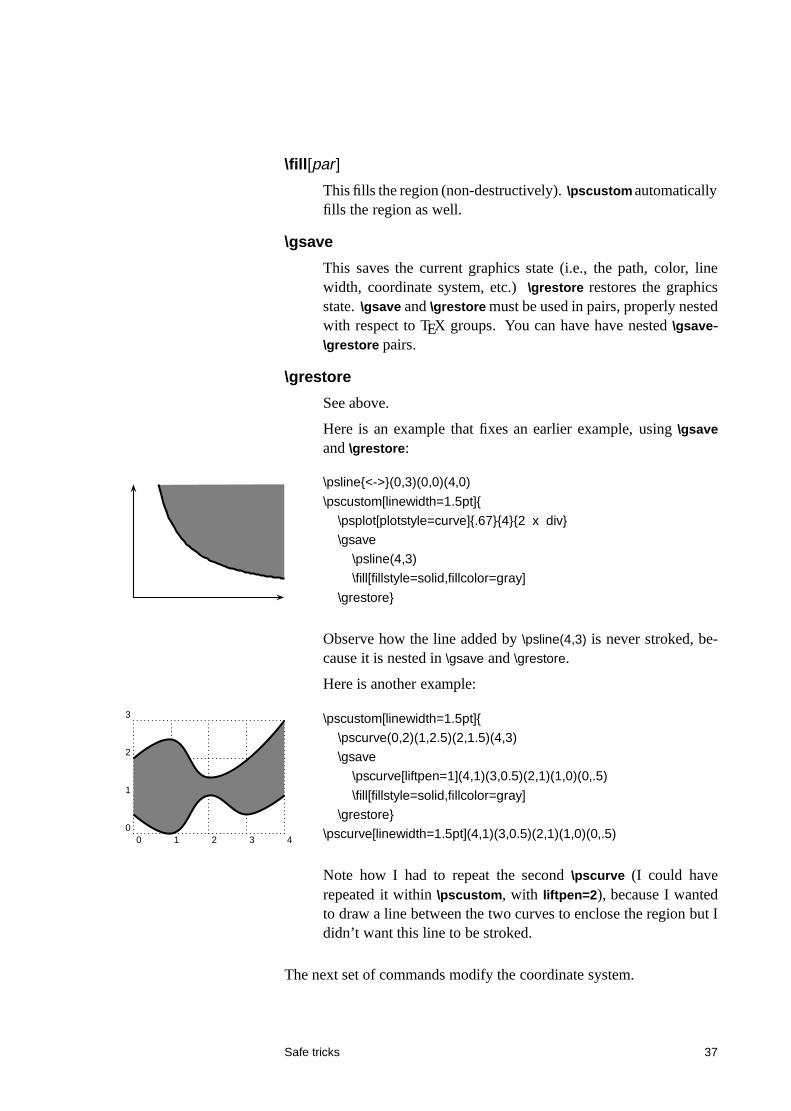
Here is another example:

0 1 2 3 40

1

2

3 \pscustom[linewidth=1.5pt]{

\pscurve(0,2)(1,2.5)(2,1.5)(4,3)

\gsave

\pscurve[liftpen=1](4,1)(3,0.5)(2,1)(1,0)(0,.5)

\fill[fillstyle=solid,fillcolor=gray]

\grestore}

\pscurve[linewidth=1.5pt](4,1)(3,0.5)(2,1)(1,0)(0,.5)

Note how I had to repeat the second \pscurve (I could haverepeated it within \pscustom, with liftpen=2), because I wantedto draw a line between the two curves to enclose the region but Ididn’t want this line to be stroked.

The next set of commands modify the coordinate system.

Safe tricks 37

\translate(coor)

Translate coordinate system by (x,y). This shifts everything thatcomes later by (x,y), but doesn’t affect what has already beendrawn.

\scale{num1 num2}

Scale the coordinate system in both directions by num1, or hori-zontally by num1 and vertically by num2.

\rotate{angle}

Rotate the coordinate system by angle.

\swapaxes

Switch the x and y coordinates. This is equivalent to

\rotate{-90}

\scale{-1 1 scale}

\msave

Save the current coordinate system. You can then restore it with\mrestore. You can have nested \msave-\mrestore pairs. \msaveand \mrestore do not have to be properly nested with respect toTEX groups or \gsave and \grestore. However, remember that\gsave and \grestorealso affect the coordinate system. \msave-\mrestore lets you change the coordinate system while drawingpart of a path, and then restore the old coordinate system withoutdestroying the path. \gsave-\grestore, on the other hand, affectthe path and all other componments of the graphics state.

\mrestore

See above.

And now here are a few shadow tricks:

\openshadow[par]

Strokes a replica of the current path, using the various shadowparameters.

\closedshadow[par]

Makes a shadow of the region enclosed by the current path as ifit were opaque regions.

\movepath(coor)

Moves the path by (x,y). Use \gsave-\grestore if you don’t wantto lose the original path.

Safe tricks 38

21 Pretty safe tricks

The next group of commands are safe, as long as there is a currentpoint!

\lineto(coor)

This is a quick version of \psline(coor).

\rlineto(coor)

This is like \lineto, but (x,y) is interpreted relative to the currentpoint.

\curveto(x1,y1)(x2,y2)(x3,y3)

This is a quick version of \psbezier(x1,y1)(x2,y2)(x3,y3).

\rcurveto(x1,y1)(x2,y2)(x3,y3)

This is like \curveto, but (x1,y1), (x2,y2) and (x3,y3) are inter-preted relative to the current point.

22 For hackers only

For PostScript hackers, there are a few more commands. Be sure toread Appendix C before using these. Needless to say:

PS Warning: Misuse of the commands in this section cancause PostScript errors.

The PostScript environment in effect with \pscustom has one unit equalto one TEX pt.

\code{code}

Insert the raw PostScript code.

\dim{dim}

Convert the PSTricks dimension to the number of pt’s, and insertsit in the PostScript code.

\coor(x1,y1)(x2,y2)...(xn,yn)

Convert one or more PSTricks coordinates to a pair of numbers(using pt units), and insert them in the PostScript code.

Pretty safe tricks 39

\rcoor(x1,y1)(x2,y2)...(xn,yn)

Like \coor, but insert the coordinates in reverse order.

\file{file}

This is like \code, but the raw PostScript is copied verbatim(except comments delimited by %) from file.

\arrows{arrows}

This defines the PostScript operators ArrowA and ArrowB so that

x2 y2 x1 y1 ArrowA

x2 y2 x1 y1 ArrowB

each draws an arrow(head) with the tip at (x1,y1) and pointingfrom (x2,y2). ArrowA leaves the current point at end of the arrow-head, where a connect line should start, and leaves (x2,y2) on thestack. ArrowB does not change the current point, but leaves

x2 y2 x1’ y1’

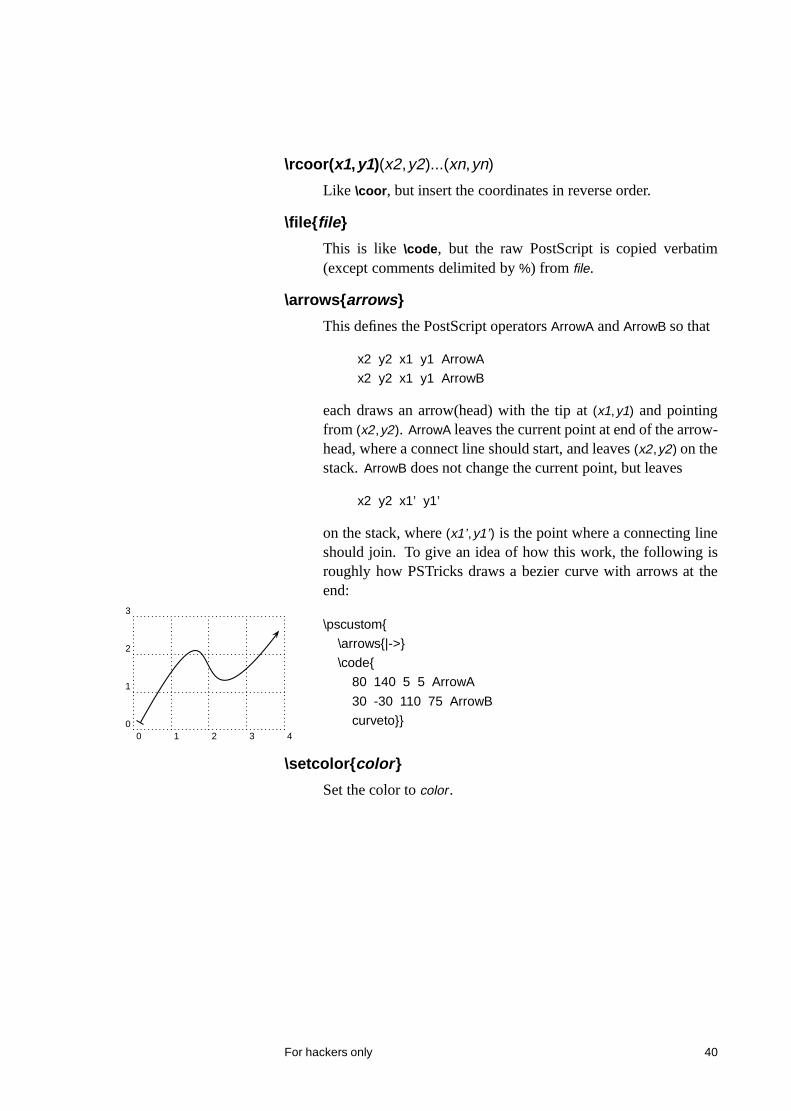
on the stack, where (x1’,y1’) is the point where a connecting lineshould join. To give an idea of how this work, the following isroughly how PSTricks draws a bezier curve with arrows at theend:

0 1 2 3 40

1

2

3

\pscustom{

\arrows{|->}

\code{

80 140 5 5 ArrowA

30 -30 110 75 ArrowB

curveto}}

\setcolor{color}

Set the color to color .

For hackers only 40

V Picture Tools

23 Pictures

The graphics objects and \rput and its variants do not change TEX’scurrent point (i.e., they create a 0-dimensional box). If you stringseveral of these together (and any other 0-dimensional objects), theyshare the same coordinate system, and so you can create a picture. Forthis reason, these macros are called picture objects.

If you create a picture this way, you will probably want to give the wholepicture a certain size. You can do this by putting the picture objects ina pspicture environment, as in:

\pspicture*[baseline](x0,y0)(x1,y1)

picture objects \endpspicture

The picture objects are put in a box whose lower left-hand corner isat (x0,y0) (by default, (0,0)) and whose upper right-hand corner is at(x1,y1).

By default, the baseline is set at the bottom of the box, but the optionalargument [baseline] sets the baseline fraction baseline from the bottom.Thus, baseline is a number, generally but not necessarily between 0 and1. If you include this argument but leave it empty ([ ]), then the baselinepasses through the origin.

Normally, the picture objects can extend outside the boundaries of thebox. However, if you include the *, anything outside the boundaries isclipped.

Besides picture objects, you can put anything in a \pspicture that doesnot take up space. E.g., you can put in font declarations and use \psset,and you can put in braces for grouping. PSTricks will alert you if youinclude something that does take up space.8

LaTEX users can type

8When PSTricks picture objects are included in a \pspicture environment, theygobble up any spaces that follow, and any preceding spaces as well, making it lesslikely that extraneous space gets inserted. (PSTricks objects always ignore spaces

Picture Tools 41

\begin{pspicture} … \end{pspicture}

You can use PSTricks picture objects in a LaTEX picture environment, andyou can use LaTEX picture objects in a PSTricks pspicture environment.However, the pspicture environment makes LaTEX’s picture environmentobsolete, and has a few small advantages over the latter. Note thatthe arguments of the pspicture environment work differently from thearguments of LaTEX’s picture environment (i.e., the right way versus thewrong way).

Driver notes: The clipping option (*) uses \pstVerb and \pstverbscale.

24 Placing and rotating whatever

PSTricks contains several commands for positioning and rotating anHR-mode argument. All of these commands end in put, and bear somesimilarity to LaTEX’s \putcommand, but with additional capabilities. LikeLaTEX’s \put and unlike the box rotation macros described in Section 29,these commands do not take up any space. They can be used inside andoutside \pspicture environments.

Most of the PSTricks put commands are of the form:

\put*arg{rotation}(coor){stuff }

With the optional * argument, stuff is first put in a

\psframebox*[boxsep=false]{<stuff>}

thereby blotting out whatever is behind stuff . This is useful for posi-tioning text on top of something else.

arg refers to other arguments that vary from one put command to another,The optional rotation is the angle by which stuff should be rotated; thisarguments works pretty much the same for all put commands and isdescribed further below. The (coor) argument is the coordinate forpositioning stuff , but what this really means is different for each put

command. The (coor) argument is shown to be obligatory, but you canactually omit it if you include the rotation argument.

that follow. If you also want them to try to neutralize preceding space when usedoutside the \pspicture environment (e.g., in a LaTEX picture environment), then use thecommand \KillGlue. The command \DontKillGlue turns this behavior backoff.)

Placing and rotating whatever 42

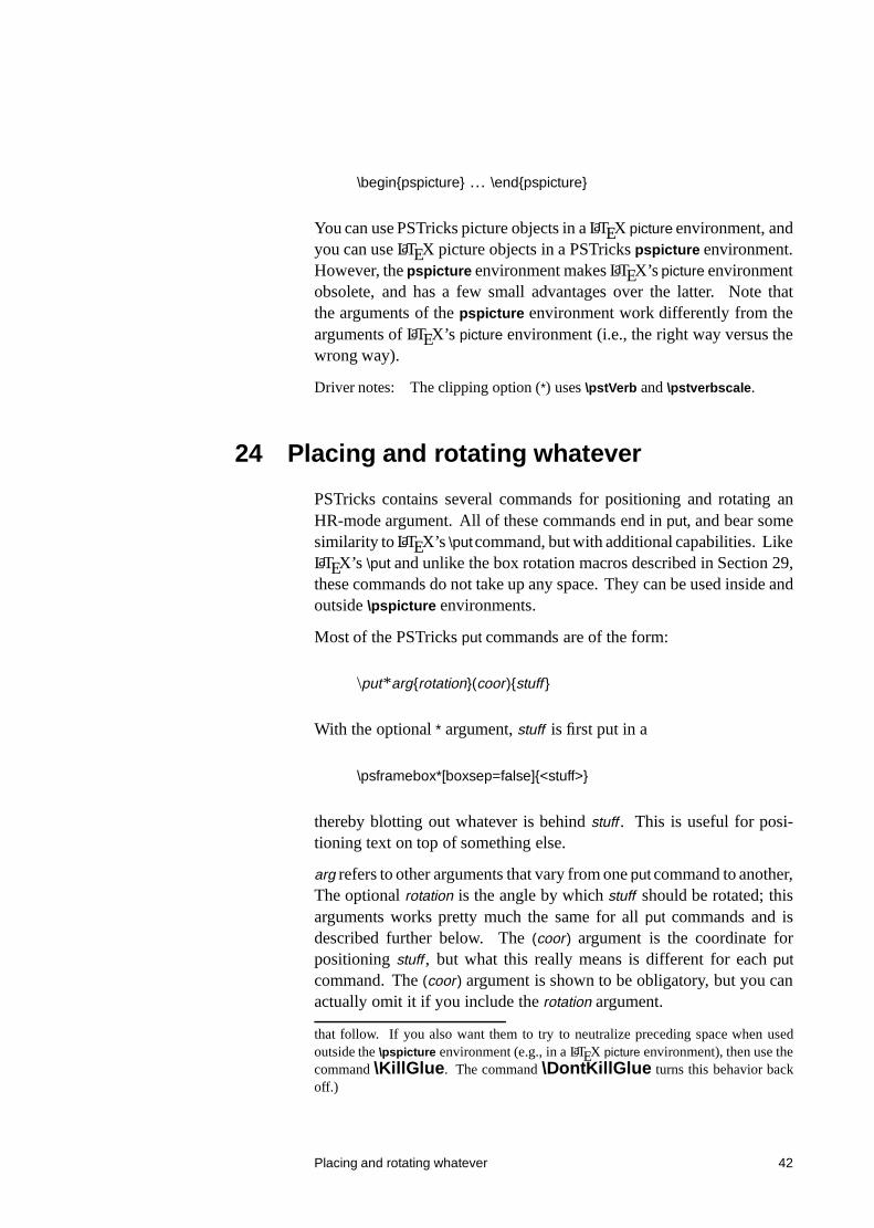
The rotation argument should be an angle, as described in Section 4,but the angle can be preceded by an *. This causes all the rotations(except the box rotations described in Section 29) within which the\rput command is be nested to be undone before setting the angle ofrotation. This is mainly useful for getting a piece of text right side upwhen it is nested inside rotations. For example,

stuff

\rput{34}{%

\psframe(-1,0)(2,1)

\rput[br]{*0}(2,1){\em stuff}}

There are also some letter abbreviations for the command angles. Theseindicate which way is up:

Letter Short for Equiv. to

U Up 0

L Left 90

D Down 180

R Right 270

Letter Short for Equiv. to

N North *0

W West *90

S South *180

E East *270

This section describes just a two of the PSTricks put commands. Themost basic one command is

\rput*[refpoint]{rotation}(x,y){stuff }

refpoint determines the reference point of stuff , and this reference pointis translated to (x,y).

By default, the reference point is the center of the box. This can bechanged by including one or two of the following in the optional refpointargument:

Horizontal Vertical

l Left t Top

r Right b Bottom

B Baseline

Visually, here is where the reference point is set of the various combi-nations (the dashed line is the baseline):

Placing and rotating whatever 43

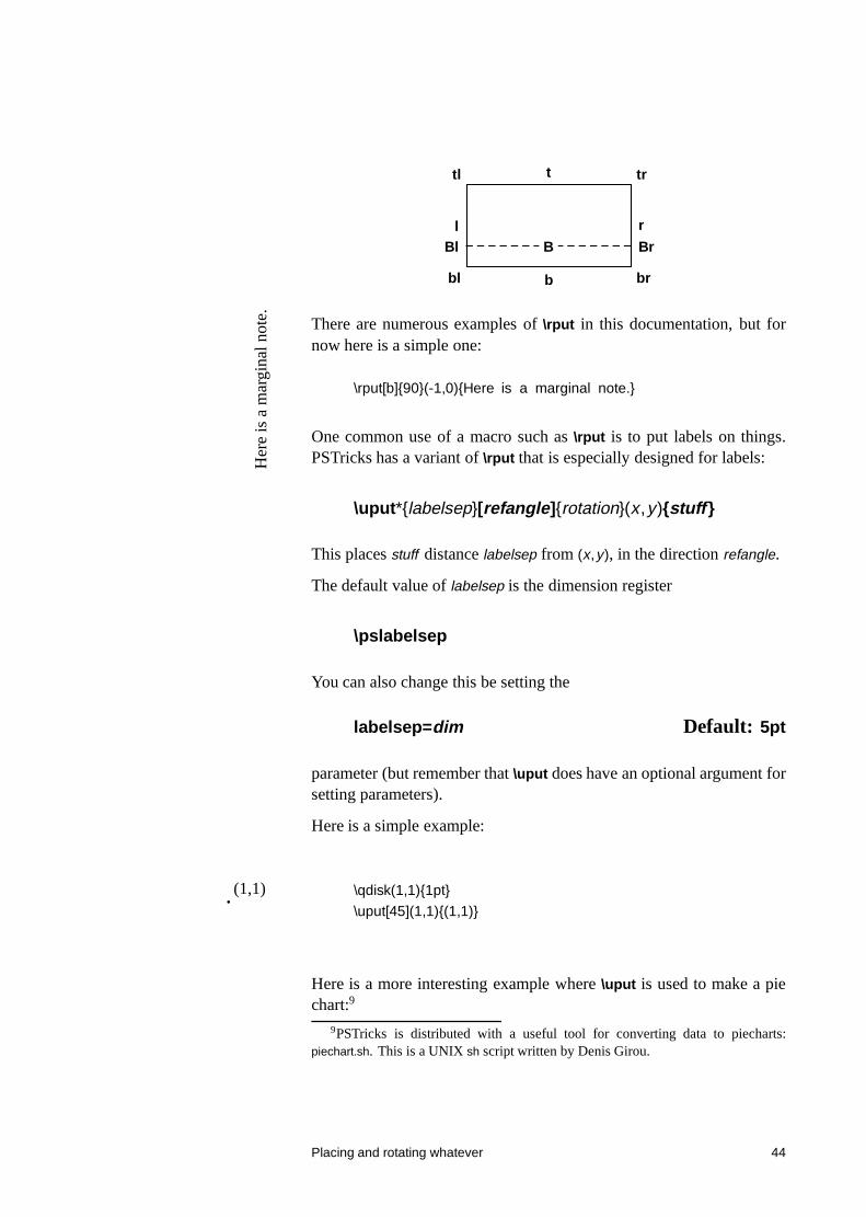
t

b

Bl

Bl

bl

tl

r

Br

br

tr

There are numerous examples of \rput in this documentation, but fornow here is a simple one:

Her

eis

am

argi

naln

ote.

\rput[b]{90}(-1,0){Here is a marginal note.}

One common use of a macro such as \rput is to put labels on things.PSTricks has a variant of \rput that is especially designed for labels:

\uput*{labelsep}[refangle]{rotation}(x,y){stuff }

This places stuff distance labelsep from (x,y), in the direction refangle.

The default value of labelsep is the dimension register

\pslabelsep

You can also change this be setting the

labelsep=dim Default: 5pt

parameter (but remember that \uput does have an optional argument forsetting parameters).

Here is a simple example:

(1,1) \qdisk(1,1){1pt}

\uput[45](1,1){(1,1)}

Here is a more interesting example where \uput is used to make a piechart:9

9PSTricks is distributed with a useful tool for converting data to piecharts:piechart.sh. This is a UNIX sh script written by Denis Girou.

Placing and rotating whatever 44

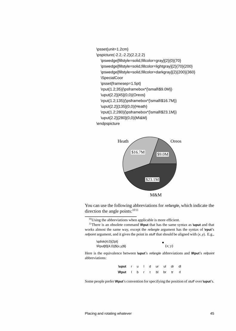
\psset{unit=1.2cm}

\pspicture(-2.2,-2.2)(2.2,2.2)

\pswedge[fillstyle=solid,fillcolor=gray]{2}{0}{70}

\pswedge[fillstyle=solid,fillcolor=lightgray]{2}{70}{200}

\pswedge[fillstyle=solid,fillcolor=darkgray]{2}{200}{360}

\SpecialCoor

\psset{framesep=1.5pt}

\rput(1.2;35){\psframebox*{\small\$9.0M}}

\uput{2.2}[45](0,0){Oreos}

\rput(1.2;135){\psframebox*{\small\$16.7M}}

\uput{2.2}[135](0,0){Heath}

\rput(1.2;280){\psframebox*{\small\$23.1M}}

\uput{2.2}[280](0,0){M\&M}

\endpspicture

$9.0M

Oreos

$16.7M

Heath

$23.1M

M&M

You can use the following abbreviations for refangle, which indicate thedirection the angle points:1011

10Using the abbreviations when applicable is more efficient.11There is an obsolete command \Rput that has the same syntax as \uput and that

works almost the same way, except the refangle argument has the syntax of \rput’srefpoint argument, and it gives the point in stuff that should be aligned with (x,y). E.g.,

\qdisk(4,0){2pt}(x; y)\Rput[tl](4,0){$(x,y)$}

Here is the equivalence between \uput’s refangle abbreviations and \Rput’s refpointabbreviations:

\uput r u l d ur ul dr dl

\Rput l b r t bl br tr rl

Some people prefer \Rput’s convention for specifying the position of stuff over \uput’s.

Placing and rotating whatever 45

Letter Short for Equiv. to

r right 0

u up 90

l left 180

d down 270

Letter Short for Equiv. to

ur up-right 45

ul up-left 135

dl down-left 225

dr down-right 315

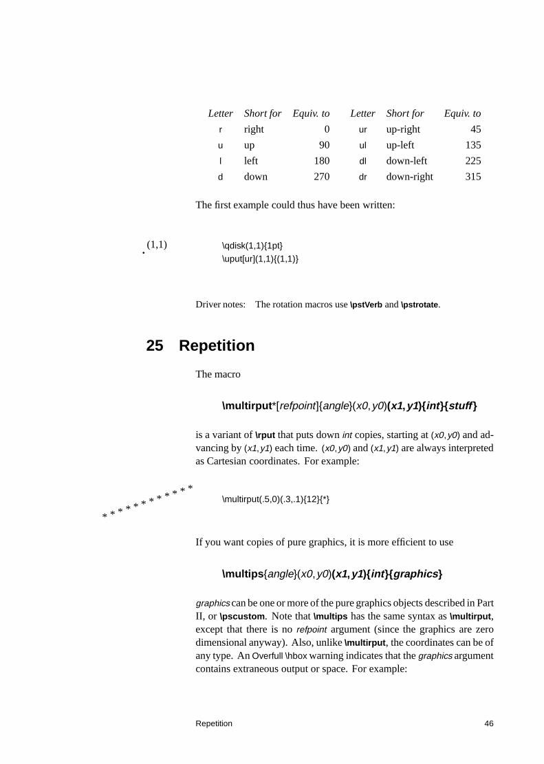
The first example could thus have been written:

(1,1) \qdisk(1,1){1pt}

\uput[ur](1,1){(1,1)}

Driver notes: The rotation macros use \pstVerb and \pstrotate.

25 Repetition

The macro

\multirput*[refpoint]{angle}(x0,y0)(x1,y1){int}{stuff }

is a variant of \rput that puts down int copies, starting at (x0,y0) and ad-vancing by (x1,y1) each time. (x0,y0) and (x1,y1) are always interpretedas Cartesian coordinates. For example:

* * * * * * * * * * * *\multirput(.5,0)(.3,.1){12}{*}

If you want copies of pure graphics, it is more efficient to use

\multips{angle}(x0,y0)(x1,y1){int}{graphics}

graphics can be one or more of the pure graphics objects described in PartII, or \pscustom. Note that \multips has the same syntax as \multirput,except that there is no refpoint argument (since the graphics are zerodimensional anyway). Also, unlike \multirput, the coordinates can be ofany type. An Overfull \hbox warning indicates that the graphics argumentcontains extraneous output or space. For example:

Repetition 46