Embed Size (px)
Citation preview
1
1BWSA-Tutorial-NLO-1
1BW
SA
Ba
rcel
on
a J
un
e 20
02
Tutorial
Nonlinear OptimizationF. Javier Heredia
Dept. of Statistics and Operational Research
Technical University of Catalonia
1BW
SA
Bar
celo
na
Jun
e 20
02
Tu
tori
al o
n N
on
linea
r O
pti
miz
atio
n
1BWSA-Tutorial-NLO-2
Motivation :Nonlinear Optimization in Statistics (I)
“All statistical procedures are, in the ultimate analysis,solutions to suitably formulated optimization problems.Whether it is designing a scientific experiment, or planning alarge-scale survey for collection of data, or choosing a stochasticmodel to characterize observed data, or drawing inference fromavailable data, such as estimation, testing of hypotheses, anddecision making, one has to choose an objective function andminimize or maximize it subject to given constraints onunknown parameters and inputs such as the costs involved.”
C.R. Rao, in “Mathematical Programming in Statistics”,
Arthanary and Dodge 1993
2
1BW
SA
Bar
celo
na
Jun
e 20
02
Tu
tori
al o
n N
on
linea
r O
pti
miz
atio
n
1BWSA-Tutorial-NLO-3
Motivation :Nonlinear Optimization in Statistics (II)
• This tutorial will be restricted to NonlinearOptimization techniques, useful for:– Maximization of a likelihood function.
– Nonlinear regression.
– ...
• We will not cover other optimization techniques as:– Combinatorial optimization.
– Global optimization.
– Nondifferentiable optimization.
– Heuristics.
• Let’s go now to the contents of this tutorial...
1BW
SA
Bar
celo
na
Jun
e 20
02
Tu
tori
al o
n N
on
linea
r O
pti
miz
atio
n
1BWSA-Tutorial-NLO-4
Decision variables
Decision variables
Constraints
Constraints[ ] 0,
),(~|),0(~
,,;
3
22
≥ℜ∈=
+⇒
ℜ∈ℜ∈ℜ∈++=
σσσσσσσσββββαααα
σσσσββββαααασσσσεεεεεεεεεεεεββββαααα
T
nn
nn
IZNZYIN
ZYZY
è
Maximization of the likelihood function
• Current status Covariates in a simple linear model (Langohr, Gómez)
– Model :
– Z is the Current Status Covariate with cumulativedistribution W(z): the only observation is whether Z exceedsthe observed value zi or not; δi is the corresponding indicatorvariable: δi = 1Z≤zi
[ ] nizy iii ,,2,1, K=δδδδ– Observations :
– Covariate : Z is supposed to be discrete with possible(ordered) values s1, s2, ..., sm and correspondingprobabilities ωj=P(Z=sj) , j=1,...,m :
[ ] ∑=
=≥=m
jjj
Tm
11 1,0,,, ωωωωωωωωωωωωωωωω Kù
3
1BW
SA
Bar
celo
na
Jun
e 20
02
Tu
tori
al o
n N
on
linea
r O
pti
miz
atio
n
1BWSA-Tutorial-NLO-5
Objective function f(x)
( )
[ ] ===
=
==
∈
−−−
= =
= =
∏∑
∏∑
otherwise],(
1 if,,1
2
1
);|(),(
1
2
1
1 1
1 1
2
2
mi
iiiIsij
j
syn
i
m
jij
n
i
m
jjjiijn
sz
zsI
e
syfL
ij
ji
δδδδγγγγ
ωωωωππππσσσσ
γγγγ
ωωωωγγγγ
σσσσββββαααα
èèù
Maximization of the likelihood function
• Maximum likelihood function :
• The problem above corresponds to a LinearlyConstrained Nonlinear Optimization Problem (LCNOP):
uxlbAxxXXxxf n
x≤≤=ℜ∈=∈ , ; )(max (LCNOP)
1BW
SA
Bar
celo
na
Jun
e 20
02
Tu
tori
al o
n N
on
linea
r O
pti
miz
atio
n
1BWSA-Tutorial-NLO-6
Decision variables x
365,,2,1
5,4,3,2,1
365
2cos),,(
K==
+
−=
j
i
cbjacbat iiiiiiij
ππππ
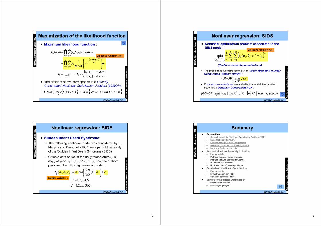
– Given a data series of the daily temperature tij inday j of year i (j=1,2,...,365 , i=1,2,...,5), the authorsproposed the following harmonic model:
Nonlinear regression: SIDS
• Sudden Infant Death Syndrome:– The following nonlinear model was considered by
Murphy and Campbell (1987) as a part of their studyof the Sudden Infant Death Syndrome (SIDS).
4
1BW
SA
Bar
celo
na
Jun
e 20
02
Tu
tori
al o
n N
on
linea
r O
pti
miz
atio
n
1BWSA-Tutorial-NLO-7
Objective function f(x)
Nonlinear regression: SIDS
• Nonlinear optimization problem associated to theSIDS model:
[ ]∑∑= ==
−5
1
365
1
2
5,,2,1,,
),,(2
1min
i jijiiiij
icba
tcbatiiiK
(Nonlinear Least-Squares Problem)
• The problem above corresponds to an Unconstrained NonlinearOptimization Problem (UNOP) :
)(min xfnx ℜ∈
(UNOP)
• If smoothness conditions are added to the model, the problembecomes a Generally Constrained NOP :
00 ≤=ℜ∈=∈ g(x)h(x)xXXxxf n
x , ; )(min (GCNOP)
1BW
SA
Bar
celo
na
Jun
e 20
02
Tu
tori
al o
n N
on
linea
r O
pti
miz
atio
n
1BWSA-Tutorial-NLO-8
Summary• Generalities
– General form of the Nonlinear Optimization Problem (NOP)– Classification of the NOP .– General strategy of the NO algorithms– Desirable properties of the NO algorithms– Local and Global optimization
• Unconstrained Nonlinear Optimization– Fundamentals– Methods that use first derivatives.– Methods that use second derivatives.– Nonderivatives methods.– Nonlinear Least-Squares problems.
• Constrained Nonlinear Optimization.– Fundamentals– Linearly constrained NOP– Generally constrained NOP
• Solvers for Nonlinear Optimization– Optimization libraries.– Modeling languages
5
1BW
SA
Bar
celo
na
Jun
e 20
02
Tu
tori
al o
n N
on
linea
r O
pti
miz
atio
n
1BWSA-Tutorial-NLO-9
Nonlinear Optimization Problem (NOP)
• The general (standard) form of the NOP is :
≤=
ℜ∈
sconstraint Inequality
sconstraint Equality
function Objective
0
0
)(
:subject to
min
)NOP(
xg
h(x)
f(x)nx
where x∈∈∈∈ℜ n are the decision variables, or simply,variables, and
lnmnn :g :h f: ℜ→ℜℜ→ℜℜ→ℜ
• Of course, max f(x) ≡≡≡≡ min –f(x)
• Usually, f, h and g are required to be differentiable and“smooth” (Lipschitz continuous, or so) to guaranteegood properties of the algorithms.
1BW
SA
Bar
celo
na
Jun
e 20
02
Tu
tori
al o
n N
on
linea
r O
pti
miz
atio
n
1BWSA-Tutorial-NLO-10
)(min 22
21 0≥+= xxxxf
x
Classification of the NOPaccordingly with the solution
• Consider the NOP expressed in the following way:
(X is known as the feasible set)
, ; )(min (NOP) 00 ≤=ℜ∈=∈ g(x)h(x)xXXxxf n
x
• NOP with optimal solution: The set f(x)|x∈X is bounded below
• Infeasible problem : the feasible set X is empty:
,1 x )(min 2122
21 0≥−≤++= xxxxxf
x
• Unbounded problem: The set f(x)|x∈X is unbounded below
)(min 22
21 0≥−−= xxxxf
x
• Existence of at least one global minimum: guaranteed if f iscontinuous and X⊆ℜn compact (Weierstrass Theorem)
6
1BW
SA
Bar
celo
na
Jun
e 20
02
Tu
tori
al o
n N
on
linea
r O
pti
miz
atio
n
1BWSA-Tutorial-NLO-11
Classification of the NOPaccordingly with the formulation
• Unconstrained NOP:
)(min xfnx ℜ∈
(UNOP)
• NOP with Simple Bounds:
)(min uxlxfx
≤≤(SBNOP)
• Linearly Constrained NOP:
uxlbAxxXXxxf n
x≤≤=ℜ∈=∈ , ; )(min (LCNOP)
• Generally Constrained NOP:
00 ≤=ℜ∈=∈ g(x)h(x)xXXxxf n
x , ; )(min (GCNOP)
1BW
SA
Bar
celo
na
Jun
e 20
02
Tu
tori
al o
n N
on
linea
r O
pti
miz
atio
n
1BWSA-Tutorial-NLO-12
• Given the feasible bounded NOP:
the general strategy followed by most of the NO alg. is:
1. Find a first feasible solution x∈X (current solution).
2. If the current solution x satisfies the optimality conditions, then
STOP: x*:=x
3. If the current solution x does not satisfies the optimality conditions,
find, using the local information available on x, a new feasible iterate
x∈X that improves the value of some merit function related with the
objective function f(x), or the objective function itself. Go to 2 with the
new current iterate.
General strategy of the NO algorithms
00 ≤=ℜ∈=∈ g(x)h(x)xXXxxf n
x , ; )(min (NOP)
7
1BW
SA
Bar
celo
na
Jun
e 20
02
Tu
tori
al o
n N
on
linea
r O
pti
miz
atio
n
1BWSA-Tutorial-NLO-13
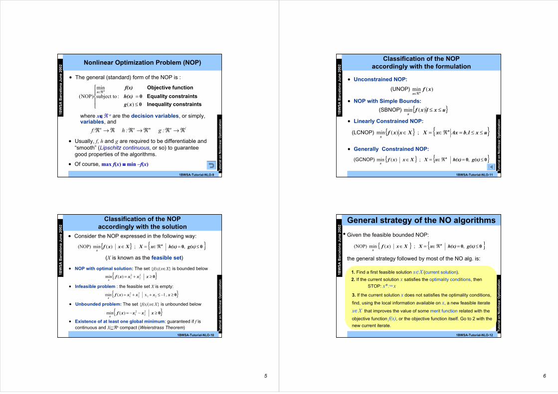
X
g(x1, x2) ≤ 0
x1
x2
Contours of f
d0 = -∇∇∇∇f(x0)’
d1 = -∇∇∇∇f(x1)’
-∇∇∇∇f(x2)’
-∇∇∇∇f(x3)’
≡≡≡≡ x*
x1= x0 + αααα0 d0
x2= x1 + αααα1 d1
x3= x2 + αααα2 d2
General strategy of the NO algorithms
x0 (initial point)
min f (x1, x2)
1BW
SA
Bar
celo
na
Jun
e 20
02
Tu
tori
al o
n N
on
linea
r O
pti
miz
atio
n
1BWSA-Tutorial-NLO-14
Desirable properties of the NOalgorithms
• Robustness: they should perform well...… on a wide variety of problems in their class
… for all reasonable choices of the initial variables
…without the need of “tuning”.
• Efficiency: low execution time and memoryrequirements
• Accuracy: they should be able to identify thesolution with precision without being affectedby errors in the data or arithmetic roundingerrors.
8
1BW
SA
Bar
celo
na
Jun
e 20
02
Tu
tori
al o
n N
on
linea
r O
pti
miz
atio
n
1BWSA-Tutorial-NLO-15
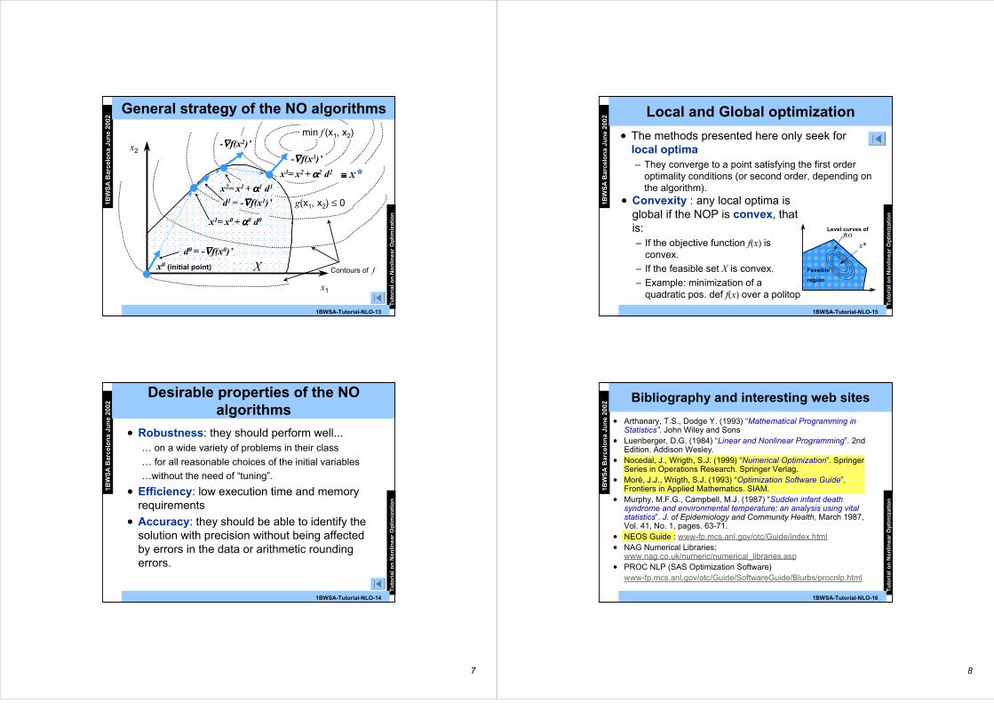
Local and Global optimization
• The methods presented here only seek forlocal optima– They converge to a point satisfying the first order
optimality conditions (or second order, depending onthe algorithm).
Level curves off(x)
x*
Feasible
region
• Convexity : any local optima isglobal if the NOP is convex, thatis:– If the objective function f(x) is
convex.
– If the feasible set X is convex.
– Example: minimization of aquadratic pos. def f(x) over a politop
1BW
SA
Bar
celo
na
Jun
e 20
02
Tu
tori
al o
n N
on
linea
r O
pti
miz
atio
n
1BWSA-Tutorial-NLO-16
• Arthanary, T.S., Dodge Y. (1993) “Mathematical Programming inStatistics”. John Wiley and Sons
• Luenberger, D.G. (1984) “Linear and Nonlinear Programming”. 2ndEdition. Addison Wesley.
• Nocedal, J., Wrigth, S.J. (1999) “Numerical Optimization”. SpringerSeries in Operations Research. Springer Verlag.
• Moré, J.J., Wrigth, S.J. (1993) “Optimization Software Guide”.Frontiers in Applied Mathematics. SIAM.
• Murphy, M.F.G., Campbell, M.J. (1987) “Sudden infant deathsyndrome and environmental temperature: an analysis using vitalstatistics”. J. of Epidemiology and Community Health, March 1987,Vol. 41, No. 1, pages. 63-71.
• NEOS Guide : www-fp.mcs.anl.gov/otc/Guide/index.html• NAG Numerical Libraries:
www.nag.co.uk/numeric/numerical_libraries.asp• PROC NLP (SAS Optimization Software)
www-fp.mcs.anl.gov/otc/Guide/SoftwareGuide/Blurbs/procnlp.html
Bibliography and interesting web sites

9
1BW
SA
Bar
celo
na
Jun
e 20
02
Tu
tori
al o
n N
on
linea
r O
pti
miz
atio
n
1BWSA-Tutorial-NLO-17

1
1BWSA-Tutorial-UNO-1
1BW
SA
Ba
rcel
on
a J
un
e 20
02
Algorithms for Unconstrained
Nonlinear Optimization
1BW
SA
Bar
celo
na
Jun
e 20
02
Un
con
stra
ined
No
nlin
ear
Op
tim
izat
ion
1BWSA-Tutorial-UNO-2
Unconstrained Nonlinear Optimization
• Fundamentals– General framework: optimality conditions; descent directions;
linesearch
– Measures of performance of the algorithms: global convergence; localconvergence.
• Methods that use first derivatives– Steepest Descent method (SD)
– Conjugate Gradient method (CG)
– Quasi-Newton method (QN)
• Methods that use second derivatives– Newton and Modified Newton methods (N, MN)
• Nonderivative methods– Finite differences, coordinate descent and direct search.
• Nonlinear Least-squares problems:– Gauss-Newton method (GN).
2
1BW
SA
Bar
celo
na
Jun
e 20
02
Un
con
stra
ined
No
nlin
ear
Op
tim
izat
ion
1BWSA-Tutorial-UNO-3
Fundamentals:
General Framework
1. Initialize xk ∈ X ≡ ℜ n (current solution). k:=02. If the current solution xk satisfies the stopping criterium, then
x*:=xk. STOP:
3. If xk is not the optimal solution, find a new iterate that improves
enough the value of the objective function, and take it as the
new iterate. This is performed through the following steps:
3.1. Computation of a descent direction d k
3.2. Computation of a steplength ααααk
3.3. Update: xk+1:= xk + ααααk d k, k:=k+1. Go to 2
Given , generate a sequence
that converges to the optimal solution x*
)(min (UNOP) xfnx ℜ∈
∞=0kk x
1BW
SA
Bar
celo
na
Jun
e 20
02
Un
con
stra
ined
No
nlin
ear
Op
tim
izat
ion
1BWSA-Tutorial-UNO-4
Usual stopping criterium
Fundamentals:
Stopping criterium: optimality conditions
• First-Order Necessary Conditions“If x* is a local minimizer and f is continuously differentiable in anopen neighbourhood of x* , then ∇f(x*)=0”
• Second-Order Necessary Conditions“If x* is a local minimizer and f and ∇ 2f is continuous in an openneighbourhood of x* , then ∇f(x*)=0 and ∇ 2f(x*) is positivesemidefinite”
• Second-Order Sufficient Conditions.“Suppose that ∇ 2f is continuous in an open neighbourhood of x*and that ∇f(x*)=0 and ∇ 2f(x*) is positive definite. Then x* is astrict local minimizer and f ”
• The role of convexity.“When f is convex, any local minimizer x* is a global minimizerof f . If, in addition, f is differentiable, then any stationarypoint x* is a global minimizer of f ”
3
1BW
SA
Bar
celo
na
Jun
e 20
02
Un
con
stra
ined
No
nlin
ear
Op
tim
izat
ion
1BWSA-Tutorial-UNO-5
Fundamentals:
Practical stopping criterium
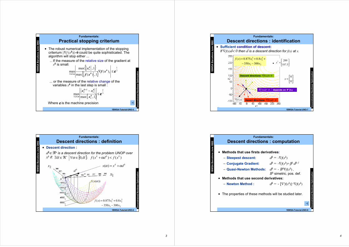
• The robust numerical implementation of the stoppingcriterium ||∇f (xk)||≈0 could be quite sophisticated. Thealgorithm will stop either ...... If the measure of the relative size of the gradient at
xk is small: 3
1
1)(
1,)(max
1,maxmax εεεε≤∇≤≤ i
k
k
ki
nixf
xf
x
Where εεεε is the machine precision
... or the measure of the relative change of thevariables xk in the last step is small :
3
21
1 1,maxmax εεεε≤
−+
≤≤ ki
ki
ki
ni x
xx
1BW
SA
Bar
celo
na
Jun
e 20
02
Un
con
stra
ined
No
nlin
ear
Op
tim
izat
ion
1BWSA-Tutorial-UNO-6
Fundamentals:
Descent directions : definition
1x
2x
kx
21
22
21
300350
8.0875.0)(
xx
xxxf
−−+=
kk dxx αα +=)(
))(( αxf
• Descent direction :
dk∈ℜn is a descent direction for the problem UNOP overxk if: [ ] )()( :,0 kkk xfdxf <+∈∀ℜ∈∃ + αααα
kd
4
1BW
SA
Bar
celo
na
Jun
e 20
02
Un
con
stra
ined
No
nlin
ear
Op
tim
izat
ion
1BWSA-Tutorial-UNO-7
=
5.187
200*x21
22
21
300350
8.0875.0)(
xx
xxxf
−−++=
Fundamentals:
Descent directions : identification
Ascent directions: ∇f(x)d> 0
Descent directions: ∇f(x)d< 0
∇f (x)d= 0 : depends on ∇∇∇∇ 2f(x)
• Sufficient condition of descent:If ∇f(x)d< 0 then d is a descent direction for f(x) at x.
)(xf∇
=
0
0x
x
1BW
SA
Bar
celo
na
Jun
e 20
02
Un
con
stra
ined
No
nlin
ear
Op
tim
izat
ion
1BWSA-Tutorial-UNO-8
Fundamentals:
Descent directions : computation
• Methods that use firsts derivatives:
– Steepest descent: dk = -∇f(xk)
– Conjugate Gradient: dk = -∇f(xk)+βk dk-1
– Quasi-Newton Methods: dk = - Bk∇f(xk) ,Bk simetric, pos. def.
• Methods that use second derivatives:
– Newton Method : dk = - [∇2f(xk)]-1∇f(xk)
• The properties of these methods will be studied later.
5
1BW
SA
Bar
celo
na
Jun
e 20
02
Un
con
stra
ined
No
nlin
ear
Op
tim
izat
ion
1BWSA-Tutorial-UNO-9
Fundamentals:
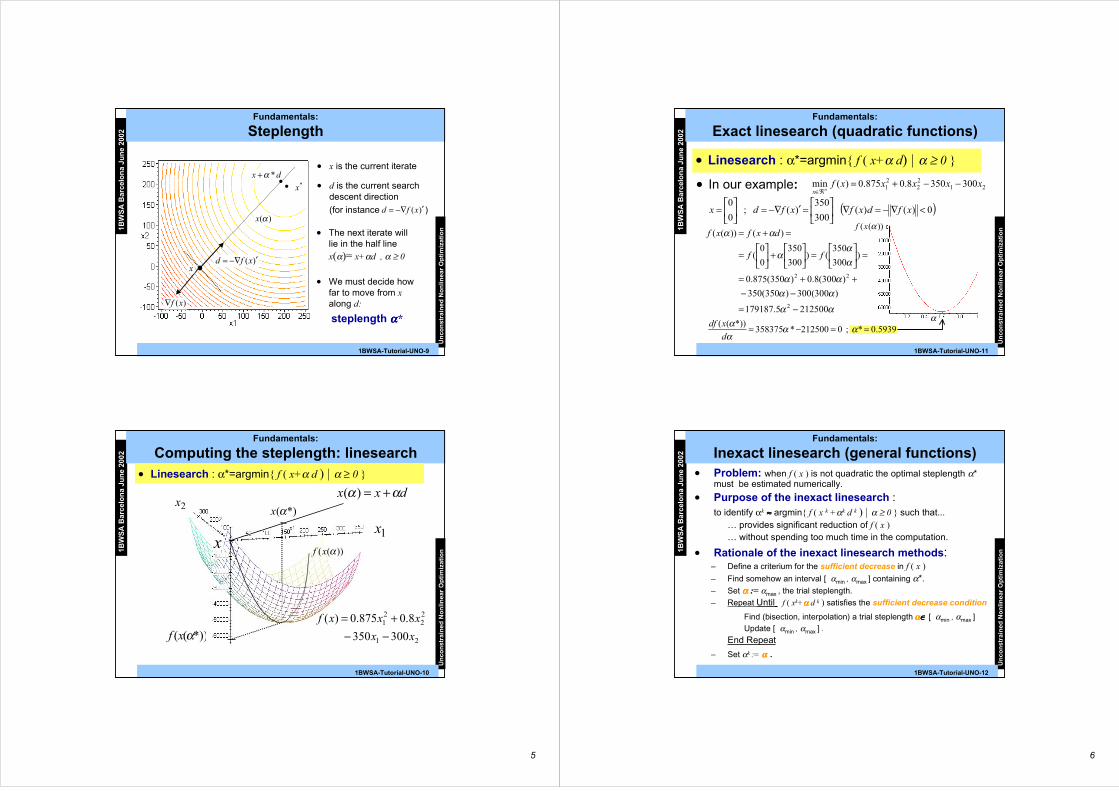
Steplength
)(xf∇
• x is the current iterate
*x
x
dx *α+
• We must decide howfar to move from xalong d:
steplength αααα*
)(αx
• The next iterate willlie in the half line
x(α)= x+αd , α ≥ 0)( ′−∇= xfd
• d is the current searchdescent direction
(for instance ))( ′−∇= xfd
1BW
SA
Bar
celo
na
Jun
e 20
02
Un
con
stra
ined
No
nlin
ear
Op
tim
izat
ion
1BWSA-Tutorial-UNO-10
1x
2x
x
21
22
21
300350
8.0875.0)(
xx
xxxf
−−+=
*)(αx
*))(( αxf
Fundamentals:
Computing the steplength: linesearch• Linesearch : α*=argmin f ( x+α d ) | α ≥ 0
dxx αα +=)(
))(( αxf
6
1BW
SA
Bar
celo
na
Jun
e 20
02
Un
con
stra
ined
No
nlin
ear
Op
tim
izat
ion
1BWSA-Tutorial-UNO-11
Fundamentals:
Exact linesearch (quadratic functions)
• Linesearch : α*=argmin f ( x+α d) | α ≥ 0
αα
αααα
αα
α
αα
2125005.179187
)300(300)350(350
)300(8.0)350(875.0
)300
350()
300
350
0
0(
)())((
2
22
−=
−−++=
=
=
+
=
=+=
ff
dxfxf
α
))(( αxf
( )0)()( 300
350)( ;
0
0<∇−=∇
=′−∇=
= xfdxfxfdx
2122
21 3003508.0875.0)( min xxxxxf
nx−−+=
ℜ∈• In our example:
5939.0* ; 0212500*358375*))(( ==−= αα
αα
d
xdf
1BW
SA
Bar
celo
na
Jun
e 20
02
Un
con
stra
ined
No
nlin
ear
Op
tim
izat
ion
1BWSA-Tutorial-UNO-12
Fundamentals:
Inexact linesearch (general functions)• Problem: when f ( x ) is not quadratic the optimal steplength α*
must be estimated numerically.
• Purpose of the inexact linesearch :to identify αk ≈≈≈≈ argmin f ( x k +αk d k ) | α ≥ 0 such that...
… provides significant reduction of f ( x )… without spending too much time in the computation.
• Rationale of the inexact linesearch methods:– Define a criterium for the sufficient decrease in f ( x )– Find somehow an interval [ αmin , αmax ] containing α*.– Set αααα := αmax , the trial steplength.
– Repeat Until f ( xk+αααα d k ) satisfies the sufficient decrease condition
Find (bisection, interpolation) a trial steplength αααα∈∈∈∈ [ αmin , αmax ]
Update [ αmin , αmax ] .
End Repeat
– Set αk := αααα .

7
1BW
SA
Bar
celo
na
Jun
e 20
02
Un
con
stra
ined
No
nlin
ear
Op
tim
izat
ion
1BWSA-Tutorial-UNO-13
• Sufficient decrease condition: (Wolfe conditions)
Fundamentals:
Inexact linesearch (general functions)
)()( kk dxf αα +=Φ
α
[ ] α⋅∇+ kkk dxfcxf )()( 1
( )W1])([)()( 1 αα ⋅∇+≤+ kkkkk dxfcxfdxf
kk dxfc )(2∇
( )10
W2)()(
21
2
<<<∇≥+∇cc
dxfcddxf kkkkk α
αααα acceptable αααα acceptable
1BW
SA
Bar
celo
na
Jun
e 20
02
Un
con
stra
ined
No
nlin
ear
Op
tim
izat
ion
1BWSA-Tutorial-UNO-14
Fundamentals:
Measures of performance of an algorithm
• Global convergence: an algorithm is said to be“globally convergent” if
that is, if we can assure that the method converges toa stationary point.
– Introducing second order information, we can strengthen theresult to include convergence to a local minimum.
• Local convergence: how fast the sequence xkapproaches to the optimal solution x* .
0)(lim =∇∞→
k
kxf
8
1BW
SA
Bar
celo
na
Jun
e 20
02
Un
con
stra
ined
No
nlin
ear
Op
tim
izat
ion
1BWSA-Tutorial-UNO-15
• To ensure “global” convergence, several assumptionsmust be imposed to the objective function, the searchdirection and the steplength. Roughly speaking:
– The objective f must be bounded below andcontinuously differentiable.
– The gradient ∇∇∇∇f must be smooth (Lipschitz continuous).
– The search direction d k must be a descent direction.
– The steplengths ααααk must satisfy the Wolfe conditions.
– The angle θθθθk between the search directions d k and thesteepest descent direction -∇∇∇∇f (xk ) must be boundedaway from 90°
Fundamentals:
Global convergence
kk
kkk
dxf
dxf
)(
)(cos
∇∇−=θθθθ
xk
-∇∇∇∇f (xk )
dkθθθθk
1BW
SA
Bar
celo
na
Jun
e 20
02
Un
con
stra
ined
No
nlin
ear
Op
tim
izat
ion
1BWSA-Tutorial-UNO-16
• Zoutendijk’s theorem:Consider any iteration of the form xk+1:= xk + αk dk where dk is adescent direction and ααααk satisfies the Wolfe conditions.Suppose that f is bounded below in ℜ n and that f iscontinuously differentiable in an open set N containing the levelset
where x0 is the starting point of the iteration. Assume also that thegradient is Lipschitz continuous in N, that is, there exists aconstant L > 0 such that:
Then
Fundamentals:
Conditions for “global” convergence
)()(: 0xfxfxL ≤=
)( )(cos2
0
2 condition Zoutendijkxfk
kk ∞<∇∑≥
θθθθ
NxxxxLxfxf ∈−≤∇−∇ ~, allfor ,~)~()(

9
1BW
SA
Bar
celo
na
Jun
e 20
02
Un
con
stra
ined
No
nlin
ear
Op
tim
izat
ion
1BWSA-Tutorial-UNO-17
Fundamentals:
Interpretation of the Zoutendijk condition
• The Zoutendijk condition implies:
0)(cos22 →∇ kk xfθθθθ
• If the method for choosing the search directiond k ensures that the angle θθθθ k is bounded awayfrom 90°, then there is a positive constant δsuch that:
kk ∀>≥ 0cos δδδδθθθθ
then, it follows from (1) that:
0)(lim =∇∞→
k
kxf
(1)
1BW
SA
Bar
celo
na
Jun
e 20
02
Un
con
stra
ined
No
nlin
ear
Op
tim
izat
ion
1BWSA-Tutorial-UNO-18
Fundamentals:
Linear and superlinear order of convergence
• Linear convergence:
let xk be a sequence in ℜ n that converges tox* . We say that the convergence is Q-linear (orsimply linear) if there is a constant r∈(0,1) (ratioof convergence) such that
large lysufficient all for , krxx
xx
k
k
*
*1
≤−
−+
• The convergence is said to be Q-superlinear if
0*
*lim
1
=−
−+
∞→ xx
xx
k
k
k
10
1BW
SA
Bar
celo
na
Jun
e 20
02
Un
con
stra
ined
No
nlin
ear
Op
tim
izat
ion
1BWSA-Tutorial-UNO-19
Fundamentals:
Quadratic order of convergence
• Quadratic convergence:
let xk be a sequence in ℜ n that converges tox*. We say that the convergence is Q-quadratic(or simply quadratic) if there is a constant M>0such that :
large lysufficient all for , kMxx
xxk
k
*
*
2
1
≤−
−+
1BW
SA
Bar
celo
na
Jun
e 20
02
Un
con
stra
ined
No
nlin
ear
Op
tim
izat
ion
1BWSA-Tutorial-UNO-20
xk
x*
Fundamentals:
Order of convergence: example
......
0,0009765610
0,00000001270,0000000028
xk= 1+2-2k-1
(Quadratic)
xk= 1+k-k
(Superlinear)
xk=1+2-k
(Linear)k
0,000000000,001953139
0,000000060,003906258
0,000001210,007812507
0,000000000,000021430,015625006
0,000015260,000320000,031250005
0,003906250,003906250,062500004
0,062500000,037037040,125000003
0,250000000,250000000,250000002
0,500000001,000000000,500000001
*xxk −
11
1BW
SA
Bar
celo
na
Jun
e 20
02
Un
con
stra
ined
No
nlin
ear
Op
tim
izat
ion
1BWSA-Tutorial-UNO-21
Fundamentals
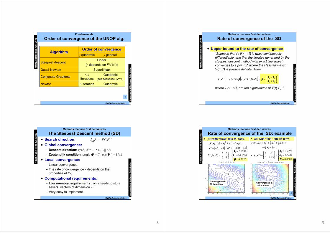
Order of convergence of the UNOP alg.
Quadratic(sub-sequence xk+n)
≤ niterations
Conjugate Gradients
Order of convergenceAlgorithm
1 iteration
f quadratic
Quadratic
Superlinear
Linear
(r depends on ∇2f (x*))
f general
Newton
Quasi-Newton
Steepest descent
1BW
SA
Bar
celo
na
Jun
e 20
02
Un
con
stra
ined
No
nlin
ear
Op
tim
izat
ion
1BWSA-Tutorial-UNO-22
Methods that use first derivatives
The Steepest Descent method (SD)• Search direction: dSD
k = -∇f (xk)’
• Global convergence:– Descent direction: ∇f (xk) dk = -|| ∇f (xk) || < 0
– Zoutendijk condition: angle θθθθk = 0°, cos(θθθθk ) = 1 ∀k
• Local convergence:– Linear convergence.
– The rate of convergence r depends on theproperties of f(x)
• Computational requirements:– Low memory requirements : only needs to store
several vectors of dimension n
– Very easy to implement.
12
1BW
SA
Bar
celo
na
Jun
e 20
02
Un
con
stra
ined
No
nlin
ear
Op
tim
izat
ion
1BWSA-Tutorial-UNO-23
Methods that use first derivatives
Rate of convergence of the SD
• Upper bound to the rate of convergence“Suppose that f : ℜ n → ℜ is twice continuouslydifferentiable, and that the iterates generated by thesteepest descent method with exact line searchconverges to a point x* where the Hessian matrix∇2f( x*) is positive definite. Then:
where λ1≤... ≤ λn are the eigenvalues of ∇2f( x*) “
[ ] ; *)()(*)()(
2
1
11
+−=−≤−+
λλλλλλλλλλλλλλλλββββββββ
n
nkk xfxfxfxf
1BW
SA
Bar
celo
na
Jun
e 20
02
Un
con
stra
ined
No
nlin
ear
Op
tim
izat
ion
1BWSA-Tutorial-UNO-24
===
=∇
7025.0
1098.10
8902.0
; 93
32*)( 2
12
ββββλλλλλλλλ
xf
Methods that use first derivatives
Rate of convergence of the SD: example• f(x) with “slow” rate of conv.
213
22
121 3),( xxxxxxf ++=
[ ]′−−= 130x
• f(x) with “fast” rate of conv.
2169
1415
21213
2432
121 ),(
xx
xxxxxxf
−+
+++=
===
=∇
0588.0
6404.2
6096.1
; 25.25.
5.2*)( 2
12
ββββλλλλλλλλ
xf
-4 -3.5 -3 -2.5 -2 -1.5 -1 -0.5 0-1
-0.5
0
0.5
1
1.5
2
2.5
f ( x1, x2 ) = x12 + x2
3 + 3*x1*x2
x1
LOCAL MINIMA
x 2
Convergence in55 iterations
-4 -3.5 -3 -2.5 -2 -1.5 -1 -0.5 0-1
-0.5
0
0.5
1
1.5
2
2.5
f ( x1, x
2 ) = x
12 + .75*x
23 + .5x
1x
2 + (15/4)x
1 - (9/16)*x
2
x1
LOCAL MINIMA
x 2
Convergence in18 iterations
[ ]′−= 5.125.2*x
13
1BW
SA
Bar
celo
na
Jun
e 20
02
Un
con
stra
ined
No
nlin
ear
Op
tim
izat
ion
1BWSA-Tutorial-UNO-25
Methods that use first derivatives
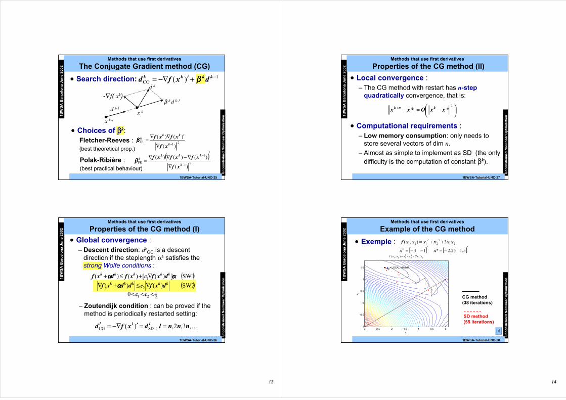
The Conjugate Gradient method (CG)
21FR
)(
)()(−∇
′∇∇=k
kkk
xf
xfxfββββ• Choices of ββββk:
Fletcher-Reeves :(best theoretical prop.)
( )21
1
PR
)(
)()()(−
−
∇
′∇−∇∇=
k
kkkk
xf
xfxfxfββββPolak-Ribière :(best practical behaviour)
• Search direction: 1CG )( −+′−∇= kkkk dxfd ββββ
x k
x k-1
d k-1
β k d k-1-∇f( xk)
d k
1BW
SA
Bar
celo
na
Jun
e 20
02
Un
con
stra
ined
No
nlin
ear
Op
tim
izat
ion
1BWSA-Tutorial-UNO-26
Methods that use first derivatives
Properties of the CG method (I)
– Zoutendijk condition : can be proved if themethod is periodically restarted setting:
K,3,2,,)( SDCG nnnldxfd lll ==′−∇=
( )( )
21
21
2
1
0SW2)()(
SW1])([)()(
<<<∇≤+∇∇+≤+
ccdxfcddxf
dxfcxfdxfkkkkk
kkkkk
αααααααααααα
• Global convergence :– Descent direction: dk
GC is a descentdirection if the steplength αk satisfies thestrong Wolfe conditions :
14
1BW
SA
Bar
celo
na
Jun
e 20
02
Un
con
stra
ined
No
nlin
ear
Op
tim
izat
ion
1BWSA-Tutorial-UNO-27
Methods that use first derivatives
Properties of the CG method (II)
• Local convergence :– The CG method with restart has n-step
quadratically convergence, that is:
−=−+ 2** xxOxx knk
• Computational requirements :– Low memory consumption: only needs to
store several vectors of dim n.
– Almost as simple to implement as SD (the onlydifficulty is the computation of constant βk).
1BW
SA
Bar
celo
na
Jun
e 20
02
Un
con
stra
ined
No
nlin
ear
Op
tim
izat
ion
1BWSA-Tutorial-UNO-28
Methods that use first derivatives
Example of the CG method
213
22
121 3),( xxxxxxf ++=
[ ]′−−= 130x [ ]′−= 5.125.2*x
• Exemple :
-3 -2.5 -2 -1.5 -1 -0.5 0-1
-0.5
0
0.5
1
1.5
f ( x1, x
2 ) = x
12 + x
23 + 3*x
1*x
2
x1
LOCAL MINIMA
x2
CG method(38 iterations)
SD method(55 iterations)
15
1BW
SA
Bar
celo
na
Jun
e 20
02
Un
con
stra
ined
No
nlin
ear
Op
tim
izat
ion
1BWSA-Tutorial-UNO-29
Methods that use first derivatives
Quasi-Newton methods (QN)
• Rationale of the Newton method:
To find the next iterate xk+1 as the minimizer of thequadratic model mk(p) of f (x) around the current iterate xk:
)()(2
1)()()( 2 pmpxfppxfxfpxf kkkkk ≡∇′+∇+≈+
)(argmin pmp kk ←
• Quasi-Newton method: Applies a Newton strategy avoiding the need ofsecond derivatives by substituiting the Hessian matrix∇2f(xk) by an approximation Bk
kkk pxx +=+1
)()()()()( 122 ′∇−∇=→=′∇+∇=∇ − kkkkkkkk xfxfpxfpxfpm 0
1BW
SA
Bar
celo
na
Jun
e 20
02
Un
con
stra
ined
No
nlin
ear
Op
tim
izat
ion
1BWSA-Tutorial-UNO-30
Methods that use first derivatives
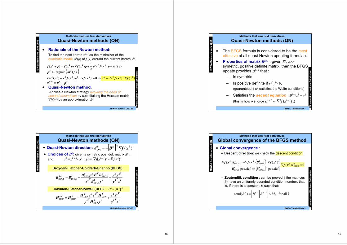
Quasi-Newton methods (QN)
• Quasi-Newton direction: [ ] )(1
QN ′∇−=− kkk xfBd
• Choices of Bk: given a symetric pos. def. matrix B0 ,
and: sk =xk +1- xk ; yk = ∇f(xk+1)’ - ∇f(xk)’
kTk
Tkk
kkTk
kTkkkkk
sy
yy
sBs
BssBBB +−=+
BFGS
BFGSBFGSBFGS
1BFGS
Broyden-Fletcher-Goldfarb-Shanno (BFGS) :
Davidon-Fletcher-Powell (DFP) : Hk =[B k]-1
kTk
Tkk
kkTk
kTkkkkk
sy
ss
yHy
HyyHHH +−=+
DFP
DFPDFPDFP
1DFP
16
1BW
SA
Bar
celo
na
Jun
e 20
02
Un
con
stra
ined
No
nlin
ear
Op
tim
izat
ion
1BWSA-Tutorial-UNO-31
Methods that use first derivatives
Quasi-Newton methods (QN)
• The BFGS formula is considered to be the mosteffective of all quasi-Newton updating formulae.
• Properties of matrix Bk+1 : given Bk, n×nsymetric, positive definite matrix, then the BFGSupdate provides Bk+1 that :
– Is symetric
– Is positive definite if sk’ yk>0.(guaranteed if αk satisfies the Wolfe conditions)
– Satisfies the secant equation : Bk+1sk = yk
(this is how we force Bk+1 ≈ ∇2f (xk+1) .)
1BW
SA
Bar
celo
na
Jun
e 20
02
Un
con
stra
ined
No
nlin
ear
Op
tim
izat
ion
1BWSA-Tutorial-UNO-32
[ ][ ] 0)(
def pos. def. pos.
)()()(BFGS1
BFGSBFGS
1
BFGSBFGS <∇
⇒
′∇−∇=∇−
−kk
kk
kkkkk
dxfBB
xfBxfdxf
• Global convergence :– Descent direction: we check the descent condition:
Methods that use first derivatives
Global convergence of the BFGS method
– Zoutendijk condition : can be proved if the matricesBk have an uniformly bounded condition number, thatis, if there is a constant M such that:
kMBBB kkk allfor ,)(cond1≤=
−
17
1BW
SA
Bar
celo
na
Jun
e 20
02
Un
con
stra
ined
No
nlin
ear
Op
tim
izat
ion
1BWSA-Tutorial-UNO-33
Methods that use first derivatives
Local convergence of the BFGS method
• Local convergence : under the followingassumptions:• The objective function f is twice continuously
differentiable
• The level set Ω= x∈ℜn : f (x) ≤ f (x0) is convex
• The objective function f has a unique minimizer x*in Ω
• The Hessian matrix ∇2f (xk+1) is Lipschitz continuousat x* and positive definite on Ω.
It can be shown that the iterates generated bythe BFGS algorithm converges superlinearlyto the minimizer x*
1BW
SA
Bar
celo
na
Jun
e 20
02
Un
con
stra
ined
No
nlin
ear
Op
tim
izat
ion
1BWSA-Tutorial-UNO-34
Methods that use first derivatives
Local convergence of the BFGS method
• Computational issues :– The efficient implementation of the BFGS method does
not store Bk explicitily, but the Cholesky factorization:
Bk = Lk Dk Lk’
– Memory consumption: n(n+1)/2 = O(n2 ) elements ofthe Cholesky factors.
– Computational cost per iteration : O(n2 ) operationsnecessary to ...
... update the Cholesky factors .
... find the solution of the linear system Bk dk= -∇f(xk ) .
– The development of an efficient implementation of theBFGS method is quite difficult.
18
1BW
SA
Bar
celo
na
Jun
e 20
02
Un
con
stra
ined
No
nlin
ear
Op
tim
izat
ion
1BWSA-Tutorial-UNO-35
Methods that use first derivatives
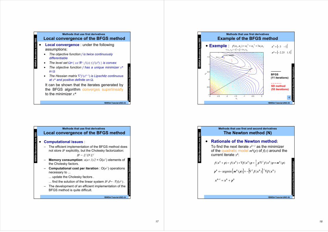
Example of the BFGS method
213
22
121 3),( xxxxxxf ++= [ ]′−−= 130x
[ ]′−= 5.125.2*x
• Exemple :
BFGS(11 iterations)
SD method(55 iterations)
-3 -2.5 -2 -1.5 -1 -0.5 0-1
-0.5
0
0.5
1
1.5
f ( x1, x2 ) = x12 + x2
3 + 3*x1*x2
x1
LOCAL MINIMA
x 2
1BW
SA
Bar
celo
na
Jun
e 20
02
Un
con
stra
ined
No
nlin
ear
Op
tim
izat
ion
1BWSA-Tutorial-UNO-36
Methods that use first and second derivatives
The Newton method (N)
• Rationale of the Newton method:To find the next iterate xk+1 as the minimizerof the quadratic model mk(p) of f(x) around thecurrent iterate xk:
)()(2
1)()()( 2 pmpxfppxfxfpxf kkkkk ≡∇′+∇+≈+
[ ] )()()( argmin12 kkkk xfxfpmp ∇∇−=←−
kkk pxx +=+1
19
1BW
SA
Bar
celo
na
Jun
e 20
02
Un
con
stra
ined
No
nlin
ear
Op
tim
izat
ion
1BWSA-Tutorial-UNO-37
-3.2 -3 -2.8 -2.6 -2.4 -2.2 -2 -1.8 -1.61
1.2
1.4
1.6
1.8
2
2.2
x1
x 2
) of (minimizer
5.1
25.2*
f
x
−=
*x
[ ]′−= 23kx
kx
211236),( 2212
22
121 +−++= xxxxxxxmk21
32
2121 3),( xxxxxxf ++=
Methods that use first and second derivatives
The Newton method (N)
• Exemple :
) of (minimizer
6.1
4.21
k
kkk
m
pxx
−=+=+
[ ]
−
=
=∇∇−=−
4.0
6.0
)()(12 kkk xfxfp
1+kx
kp
1BW
SA
Bar
celo
na
Jun
e 20
02
Un
con
stra
ined
No
nlin
ear
Op
tim
izat
ion
1BWSA-Tutorial-UNO-38
Methods that use first and second derivatives
The Newton method (N)
• Search direction: Tkkk xfxfd )()( 12N ∇−∇= −
• Global convergence :– Descent direction: the descent nature of dk
N
can only be guaranteed if the Hessianmatrix ∇∇∇∇2f(xk) is positive definite:
0)()()()(
then def. pos. )( If12
N
2
<∇∇−∇=∇
∇− Tkkkkk
k
xfxfxfdxf
xf
otherwise, the global convergence of theNewton method cannot be guaranteed.
20
1BW
SA
Bar
celo
na
Jun
e 20
02
Un
con
stra
ined
No
nlin
ear
Op
tim
izat
ion
1BWSA-Tutorial-UNO-39
Methods that use first and second derivatives
Losing of the global convergence
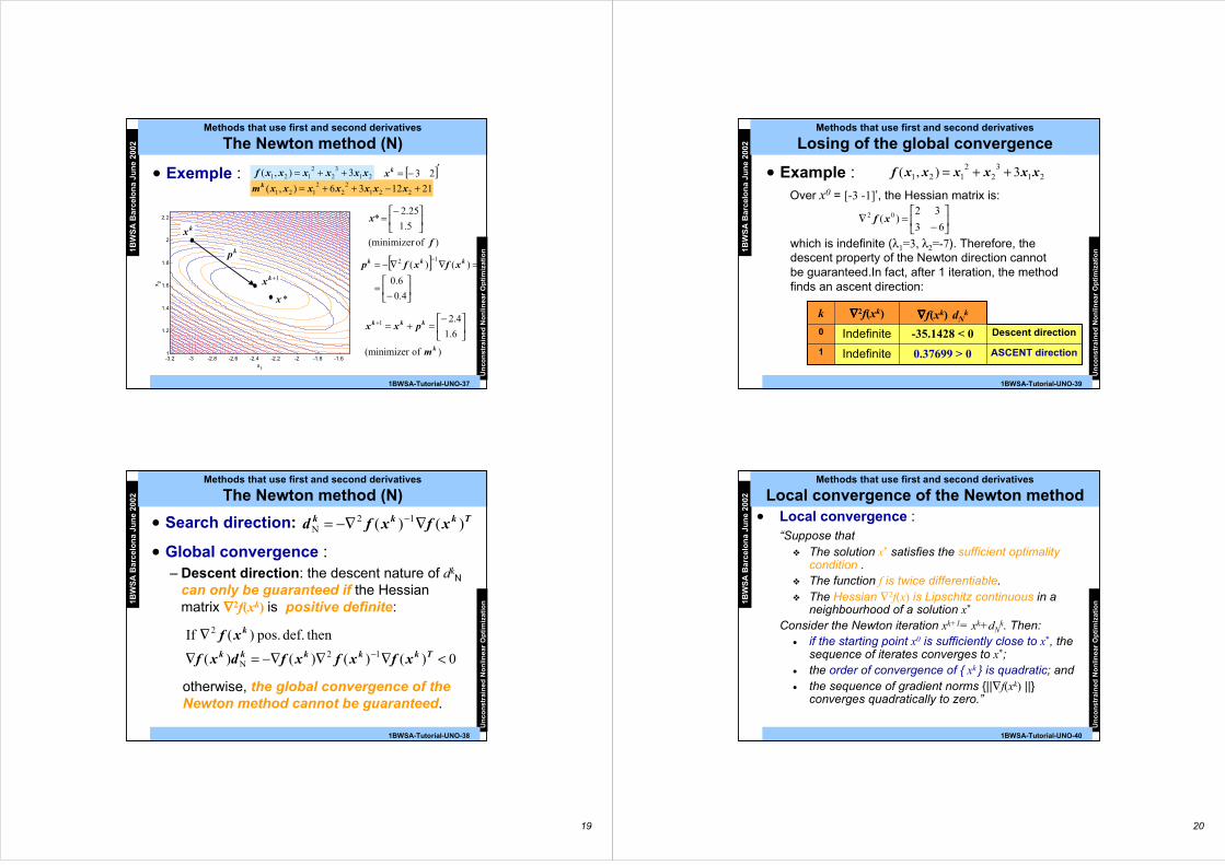
213
22
121 3),( xxxxxxf ++=• Example :Over x0 = [-3 -1]’, the Hessian matrix is:
−
=∇63
32)( 02 xf
which is indefinite (λ1=3, λ2=-7). Therefore, thedescent property of the Newton direction cannotbe guaranteed.In fact, after 1 iteration, the methodfinds an ascent direction:
0.37699 > 0
-35.1428 < 0
∇∇∇∇f(xk) dNk
ASCENT direction
Descent direction
Indefinite1
Indefinite0
∇∇∇∇2f(xk)k
1BW
SA
Bar
celo
na
Jun
e 20
02
Un
con
stra
ined
No
nlin
ear
Op
tim
izat
ion
1BWSA-Tutorial-UNO-40
Methods that use first and second derivatives
Local convergence of the Newton method• Local convergence :
“Suppose that The solution x* satisfies the sufficient optimality
condition . The function f is twice differentiable. The Hessian ∇2f(x) is Lipschitz continuous in a
neighbourhood of a solution x*
Consider the Newton iteration xk+1= xk+dNk. Then:
• if the starting point x0 is sufficiently close to x*, thesequence of iterates converges to x*;
• the order of convergence of xk is quadratic; and• the sequence of gradient norms ||∇f(xk) ||
converges quadratically to zero.”

21
1BW
SA
Bar
celo
na
Jun
e 20
02
Un
con
stra
ined
No
nlin
ear
Op
tim
izat
ion
1BWSA-Tutorial-UNO-41
Methods that use first and second derivatives
Quadratic order of convergence
≤≤≤≤≤≤≤≤≤≤≤≤≤≤≤≤
≤≤≤≤
1.702 ××××10-9
1.124 ××××10-4
3.250 ××××10-2
8.125 ××××10-1
||xk-1-x*||2
1.571××××10-9
1.029××××10-4
2.657××××10-2
4.8 ××××10-1
3.0
|| ∇∇∇∇f(xk) ||
6.296 ××××10-10
4.126 ××××10-5
1.060 ××××10-2
1.803 ××××10-1
9.013 ××××10-1
||xk-x*||
4
3
2
1
0
k
213
22
121 3),( xxxxxxf ++=• Example :
The newton method converges from x0 = [-3 2]’to x*=[-2.25 1.5]T in 4 iterations, reducing theerror ||xk-x*|| quadratically at each step :
1BW
SA
Bar
celo
na
Jun
e 20
02
Un
con
stra
ined
No
nlin
ear
Op
tim
izat
ion
1BWSA-Tutorial-UNO-42
Methods that use first and second derivatives
Modified Newton methods (MN)
• Search direction:Tkkk xfBd )(
1
MNMN ∇−=−
where BkMN=∇2f(xk)+ Ek , with
– Ek =0 if ∇2f(xk) is sufficiently positive definite;
– otherwise Ek is chosen to ensure that BkMN is
sufficiently positive definite.• Methods to compute Bk
MN : based on themodification of
– The spectral decomposition of ∇2f(xk)=QΛQT.
– The Cholesky factorization of ∇2f(xk)=LDLT.
22
1BW
SA
Bar
celo
na
Jun
e 20
02
Un
con
stra
ined
No
nlin
ear
Op
tim
izat
ion
1BWSA-Tutorial-UNO-43
• Global convergence :– Descent direction: as Bk
MN is alwayspositive definite,therefore, dk
MN is a descentsearch direction.
Methods that use first and second derivatives
Global convergence of the MN method
– Zoutendijk condition : can be proved if thematrices Bk
MN have an uniformly boundedcondition number, that is, if there is aconstant M such that :
kMBBB kkk allfor ,)(cond1
MNMNMN ≤=−
1BW
SA
Bar
celo
na
Jun
e 20
02
Un
con
stra
ined
No
nlin
ear
Op
tim
izat
ion
1BWSA-Tutorial-UNO-44
Methods that use first and second derivatives
Local convergence of the MN method
• Local convergence :
– If the sequence of iterates xk converges toa point x* where ∇2f(x*) is sufficientlypositive definite (i.e. Ek =0 for k largeenough), then the MN method reduces tothe Newton methods, and the convergenceis quadratic.
– If ∇2f(x*) is close to singular (that is, there isnot guarantee that Ek=0) the convergencerate may only be linear.
23
1BW
SA
Bar
celo
na
Jun
e 20
02
Un
con
stra
ined
No
nlin
ear
Op
tim
izat
ion
1BWSA-Tutorial-UNO-45
Methods that use first and second derivatives
Other aspects of the MN methods
• Computational issues :– The efficient implementation of the MN methods
computes and store the modified Cholesky factorizationof Bk
MN.
– Memory consumption: n(n+1)/2 = O(n2) elements ofthe Cholesky factors.
– Computational cost per iteration : O(n3) operationsnecessary to ...
... compute the modified Cholesky factors of ∇2f(x*) .
... find the solution of the linear system BkMN
dkMN= -∇f(xk )
plus the effort of computing the second derivatives
– The efficient implementation of the MN method is quitedifficult.
1BW
SA
Bar
celo
na
Jun
e 20
02
Un
con
stra
ined
No
nlin
ear
Op
tim
izat
ion
1BWSA-Tutorial-UNO-46
Methods that use first and second derivatives
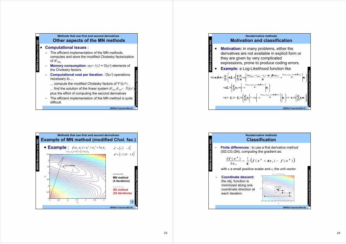
Example of MN method (modified Chol. fac.)
213
22
121 3),( xxxxxxf ++= [ ]′−−= 130x
[ ]′−= 5.125.2*x
• Example :
MN method(4 iterations)
SD method(55 iterations)
-3 -2.5 -2 -1.5 -1 -0.5 0-1
-0.5
0
0.5
1
1.5
2
2.5
f ( x1, x2 ) = x12 + x2
3 + 3*x1*x2
x1
LOCAL MINIMA
x 2
24
1BW
SA
Bar
celo
na
Jun
e 20
02
Un
con
stra
ined
No
nlin
ear
Op
tim
izat
ion
1BWSA-Tutorial-UNO-47
Nonderivative methods
Motivation and classification
• Motivation: in many problems, either thederivatives are not available in explicit form orthey are given by very complicatedexpressions, prone to produce coding errors.
• Example: a Log-Likelihood function like
−+
−−−−+
−+
−
−−−+=
∑∑
∑
∑∑
==
−−−+
=
−−−+
=
−−−+
=
m
jjiji
m
jj
sszy
ijiii
m
jj
sszy
ijii
m
jj
sszyjjiobsiobsij
ii
n
i
jjiobsiobs
jjiobsiobs
jjiobsiobs
e
e
esszy
l
11
)ln()ln(
21
1
)ln()ln(
2
1
)ln()ln(,,
11
ln)1(exp1ln)1)(1(
expln
)ln()ln(expln),,,(
,,
,,
,,
ωωωωγγγγεεεεωωωωγγγγξξξξξξξξεεεε
ωωωωγγγγξξξξεεεε
ωωωωσσσσ
ββββαααασσσσγγγγ
ξξξξεεεεσσσσββββαααα
σσσσββββαααα
σσσσββββαααα
σσσσββββαααα
ù
1BW
SA
Bar
celo
na
Jun
e 20
02
Un
con
stra
ined
No
nlin
ear
Op
tim
izat
ion
1BWSA-Tutorial-UNO-48
-3 -2.8 -2.6 -2.4 -2.2 -2 -1.8 -1.6 -1.4 -1.2 -10.5
1
1.5
2
2.5
LOCAL MINIMA
x1
x2
f ( x1, x2 ) = x12 + x2
3 + 3*x1*x2
x0
Nonderivative methods
Classification
– Finite differences : to use a first derivative method(SD,CG,QN), computing the gradient as:
– Coordinate descent:the obj. function isminimized along onecoordinate direction ateach iteration.
( ))()(1)( k
ik
i
k
xfexfx
xf −+≈∂
∂ εεεεεεεε
with ε a small positive scalar and ei the unit vector
x1
x2
x3
x4
x5
x6
x7

25
1BW
SA
Bar
celo
na
Jun
e 20
02
Un
con
stra
ined
No
nlin
ear
Op
tim
izat
ion
1BWSA-Tutorial-UNO-49
-3 -2.8 -2.6 -2.4 -2.2 -2 -1.8 -1.6 -1.4 -1.2 -10.5
1
1.5
2
LOCAL MINIMA
x1
x 2
Nonderivative methods
Classification
– Nelder & Mead simplex method :– Not to be confused with the simplex method for linear
programming.
• Start with an initialsimplex (convex hull ofn+1 points).
• Select a new point thatimproves the worst pointof the current simplex.
• Update de currentsimplex.
1BW
SA
Bar
celo
na
Jun
e 20
02
Un
con
stra
ined
No
nlin
ear
Op
tim
izat
ion
1BWSA-Tutorial-UNO-50
Nonderivative methods
Nelder & Mead method
213
22
121 3),( xxxxxxf ++= [ ]′−= 5.125.2*x• Exemple :
-3 -2.5 -2 -1.5 -1
0
0.2
0.4
0.6
0.8
1
1.2
1.4
1.6
1.8
f ( x1, x
2 ) = x
12 + x
23 + 3*x
1*x
2
x1
LOCAL MINIMA
x2
NM method(11 iterations)
26
1BW
SA
Bar
celo
na
Jun
e 20
02
Un
con
stra
ined
No
nlin
ear
Op
tim
izat
ion
1BWSA-Tutorial-UNO-51
Methods for Unconstrained Nonlinear Optimization
Computational comparison
2.506 ×10-123.344 ×10-260.2214ModifiedNewton
8.828 ×10-54.586 ×10-123.84222Nelder & Mead
0.16
0.33
1.43
120.34
Executiontime
(seconds)
2.506 ×10-123.344 ×10-2614Newton
2.793 ×10-74.980 ×10-1727Quasi-Newton
7.820 ×10-77.513 ×10-1342ConjugateGradient
9.222 ×10-61.038 ×10-114760SteepestDescent
|| ∇∇∇∇f(x*) ||f(x*)Iter.Rosenbrock
function(n=4)
1BW
SA
Bar
celo
na
Jun
e 20
02
Un
con
stra
ined
No
nlin
ear
Op
tim
izat
ion
1BWSA-Tutorial-UNO-52
The extended Rosenbrock function
The contours lines for n=2:
( ) ( )[ ]∑=
−− −+−=2/
1
212
22122 110)(
n
iiii xxxxf
-3 -2 -1 0 1 2 3-0.5
0
0.5
1
1.5
• It is considereda difficultfunction tominimize.
• Unique globalminimizer atx*=[ 1 1 ]T
27
1BW
SA
Bar
celo
na
Jun
e 20
02
Un
con
stra
ined
No
nlin
ear
Op
tim
izat
ion
1BWSA-Tutorial-UNO-53
Nonlinear Least-squares problems
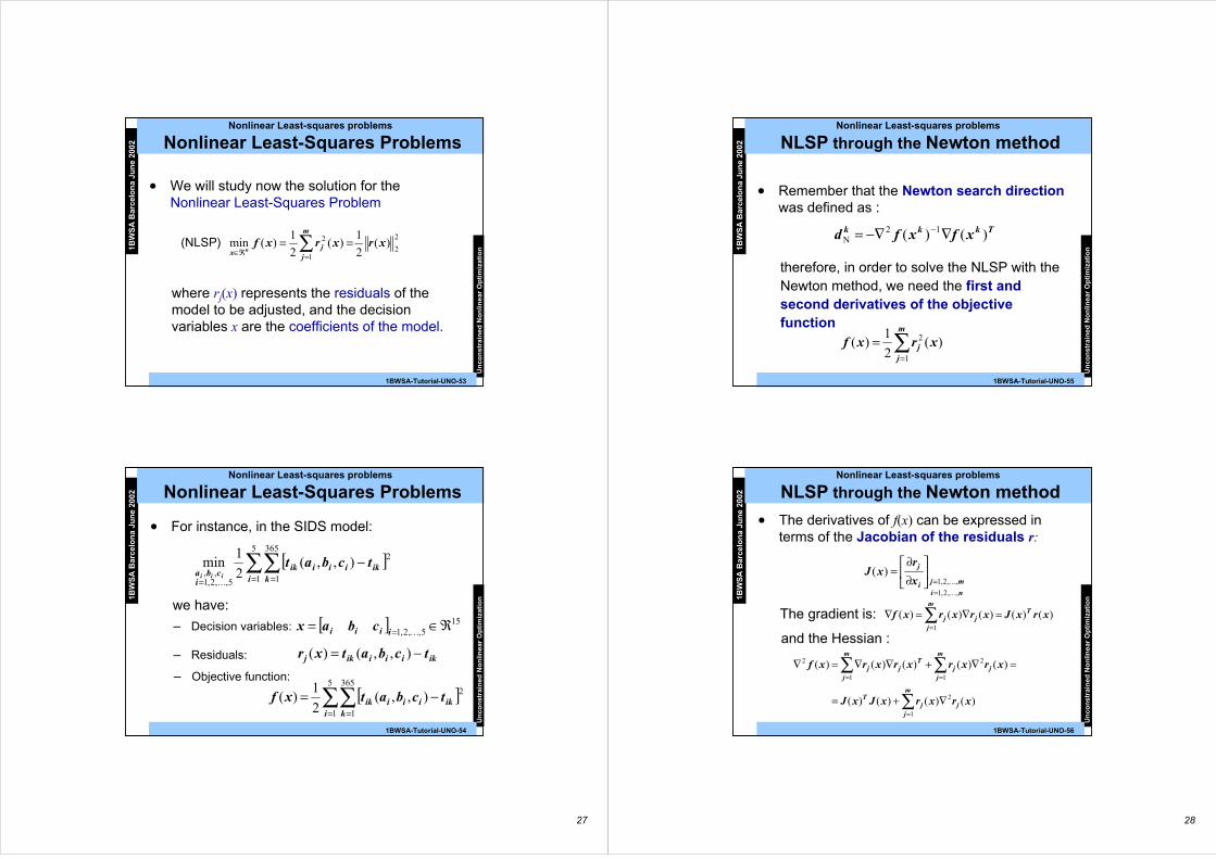
Nonlinear Least-Squares Problems
• We will study now the solution for theNonlinear Least-Squares Problem
2
21
2 )(2
1)(
2
1)(min xrxrxf
m
jj
x n ∑=ℜ∈
==(NLSP)
where rj(x) represents the residuals of themodel to be adjusted, and the decisionvariables x are the coefficients of the model.
1BW
SA
Bar
celo
na
Jun
e 20
02
Un
con
stra
ined
No
nlin
ear
Op
tim
izat
ion
1BWSA-Tutorial-UNO-54
Nonlinear Least-squares problems
Nonlinear Least-Squares Problems
• For instance, in the SIDS model:
[ ]∑∑= ==
−5
1
365
1
2
5,,2,1,,
),,(2
1min
i kikiiiik
icba
tcbatiiiK
we have:
[ ] 155,,2,1 ℜ∈= = Kiiii cbax– Decision variables:
ikiiiikj tcbatxr −= ),,()(– Residuals:
[ ]∑∑= =
−=5
1
365
1
2),,(2
1)(
i kikiiiik tcbatxf
– Objective function:
28
1BW
SA
Bar
celo
na
Jun
e 20
02
Un
con
stra
ined
No
nlin
ear
Op
tim
izat
ion
1BWSA-Tutorial-UNO-55
therefore, in order to solve the NLSP with theNewton method, we need the first andsecond derivatives of the objectivefunction
Nonlinear Least-squares problems
NLSP through the Newton method
Tkkk xfxfd )()( 12N ∇−∇= −
• Remember that the Newton search directionwas defined as :
∑=
=m
jj xrxf
1
2 )(2
1)(
1BW
SA
Bar
celo
na
Jun
e 20
02
Un
con
stra
ined
No
nlin
ear
Op
tim
izat
ion
1BWSA-Tutorial-UNO-56
Nonlinear Least-squares problems
NLSP through the Newton method
• The derivatives of f(x) can be expressed interms of the Jacobian of the residuals r:
ni
mji
j
x
rxJ
,,2,1
,,2,1)(
K
K
==
∂∂
=
∑=
=∇=∇m
j
Tjj xrxJxrxrxf
1
)()()()()(The gradient is:
∑
∑∑
=
==
∇+=
=∇+∇∇=∇
m
jjj
T
m
jjj
m
j
Tjj
xrxrxJxJ
xrxrxrxrxf
1
2
1
2
1
2
)()()()(
)()()()()(
and the Hessian :
29
1BW
SA
Bar
celo
na
Jun
e 20
02
Un
con
stra
ined
No
nlin
ear
Op
tim
izat
ion
1BWSA-Tutorial-UNO-57
A
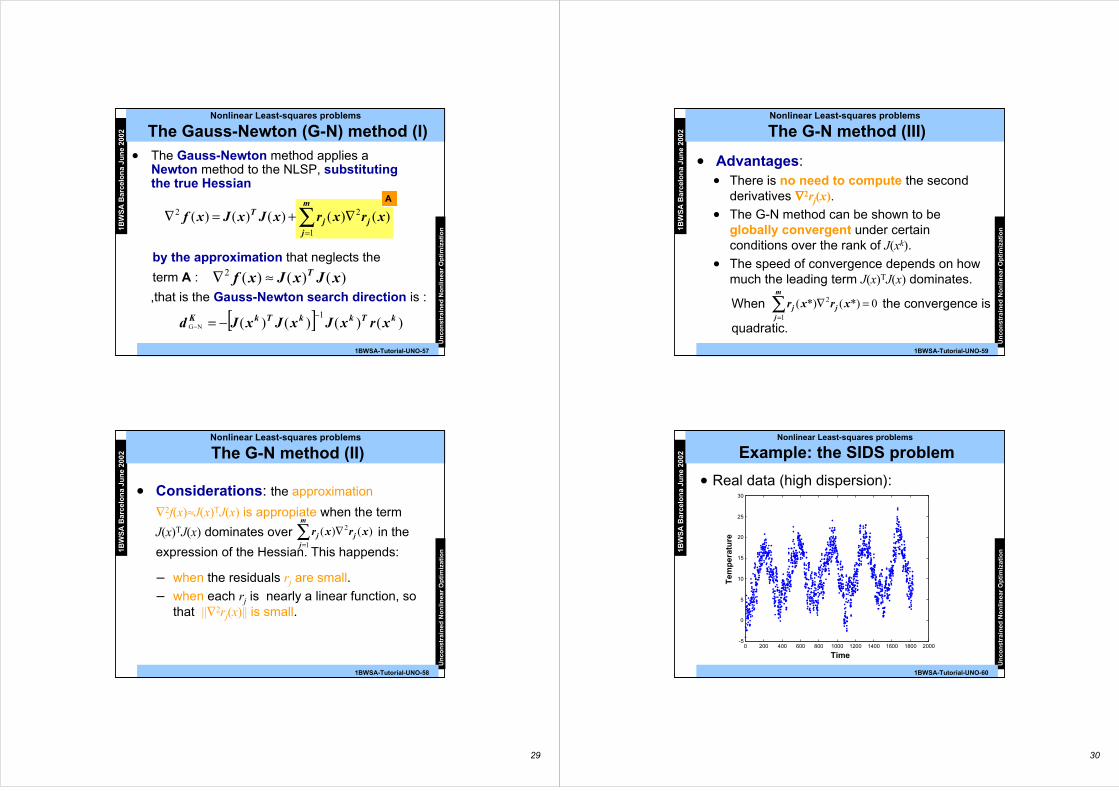
by the approximation that neglects the
term A : )()()(2 xJxJxf T≈∇
∑=
∇+=∇m
jjj
T xrxrxJxJxf1
22 )()()()()(
Nonlinear Least-squares problems
The Gauss-Newton (G-N) method (I)
• The Gauss-Newton method applies aNewton method to the NLSP, substitutingthe true Hessian
,that is the Gauss-Newton search direction is :
[ ] )()()()(1
NGkTkkTkK xrxJxJxJd
−−=−
1BW
SA
Bar
celo
na
Jun
e 20
02
Un
con
stra
ined
No
nlin
ear
Op
tim
izat
ion
1BWSA-Tutorial-UNO-58
Nonlinear Least-squares problems
The G-N method (II)
– when the residuals rj are small.
– when each rj is nearly a linear function, sothat ||∇2rj(x)|| is small.
• Considerations: the approximation
∇2f(x)≈J(x)TJ(x) is appropiate when the term
J(x)TJ(x) dominates over in the
expression of the Hessian. This happends:
∑=
∇m
jjj xrxr
1
2 )()(
30
1BW
SA
Bar
celo
na
Jun
e 20
02
Un
con
stra
ined
No
nlin
ear
Op
tim
izat
ion
1BWSA-Tutorial-UNO-59
Nonlinear Least-squares problems
The G-N method (III)
• Advantages:• There is no need to compute the second
derivatives ∇∇∇∇2rj(x).
• The G-N method can be shown to beglobally convergent under certainconditions over the rank of J(xk).
• The speed of convergence depends on howmuch the leading term J(x)TJ(x) dominates.
When the convergence is
quadratic.
∑=
=∇m
jjj xrxr
1
2 0*)(*)(
1BW
SA
Bar
celo
na
Jun
e 20
02
Un
con
stra
ined
No
nlin
ear
Op
tim
izat
ion
1BWSA-Tutorial-UNO-60
0 200 400 600 800 1000 1200 1400 1600 1800 2000-5
0
5
10
15
20
25
30
Time
Tem
pe
ratu
re
Nonlinear Least-squares problems
Example: the SIDS problem
• Real data (high dispersion):
31
1BW
SA
Bar
celo
na
Jun
e 20
02
Un
con
stra
ined
No
nlin
ear
Op
tim
izat
ion
1BWSA-Tutorial-UNO-61
Nonlinear Least-squares problems
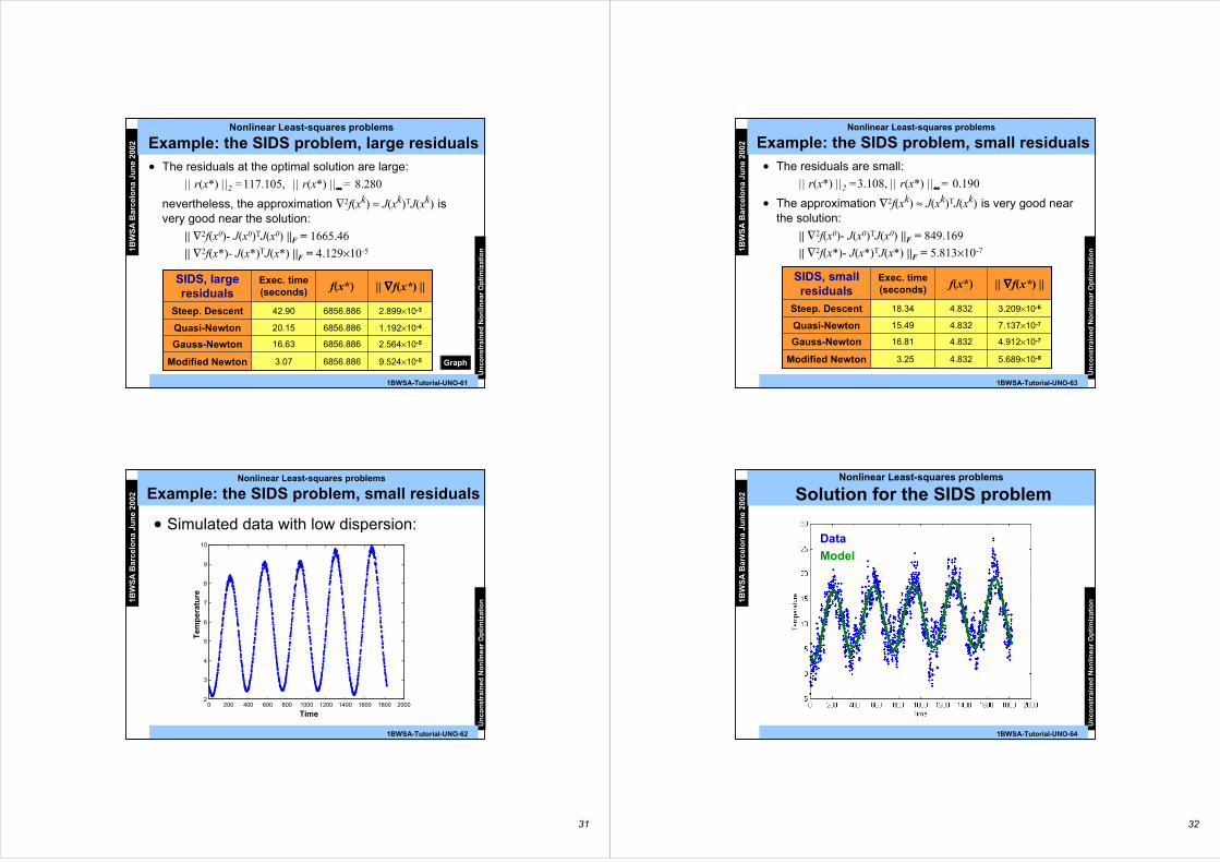
Example: the SIDS problem, large residuals
1.192×10-46856.88620.15Quasi-Newton
2.899×10-36856.88642.90Steep. Descent
2.564×10-56856.88616.63Gauss-Newton
9.524×10-56856.8863.07Modified Newton
|| ∇∇∇∇f(x*) ||Exec. time(seconds) f(x*)
SIDS, largeresiduals
• The residuals at the optimal solution are large:
|| r(x*) ||2 =117.105, || r(x*) ||∞∞∞∞ = 8.280
nevertheless, the approximation ∇2f(xk) ≈ J(xk)TJ(xk) isvery good near the solution:
|| ∇2f(x0)- J(x0)TJ(x0) ||F = 1665.46
|| ∇2f(x*)- J(x*)TJ(x*) ||F = 4.129×10⁻⁵
Graph
1BW
SA
Bar
celo
na
Jun
e 20
02
Un
con
stra
ined
No
nlin
ear
Op
tim
izat
ion
1BWSA-Tutorial-UNO-62
Nonlinear Least-squares problems
Example: the SIDS problem, small residuals
0 200 400 600 800 1000 1200 1400 1600 1800 20002
3
4
5
6
7
8
9
10
Time
Tem
per
atu
re
• Simulated data with low dispersion:
32
1BW
SA
Bar
celo
na
Jun
e 20
02
Un
con
stra
ined
No
nlin
ear
Op
tim
izat
ion
1BWSA-Tutorial-UNO-63
Nonlinear Least-squares problems
Example: the SIDS problem, small residuals
7.137×10-74.83215.49Quasi-Newton
3.209×10-64.83218.34Steep. Descent
4.912×10-74.83216.81Gauss-Newton
5.689×10-94.832 3.25Modified Newton
|| ∇∇∇∇f(x*) ||Exec. time(seconds) f(x*)
SIDS, smallresiduals
• The residuals are small:
|| r(x*) ||2 =3.108, || r(x*) ||∞∞∞∞ = 0.190
• The approximation ∇2f(xk) ≈ J(xk)TJ(xk) is very good nearthe solution:
|| ∇2f(x0)- J(x0)TJ(x0) ||F = 849.169
|| ∇2f(x*)- J(x*)TJ(x*) ||F = 5.813×10⁻⁷
1BW
SA
Bar
celo
na
Jun
e 20
02
Un
con
stra
ined
No
nlin
ear
Op
tim
izat
ion
1BWSA-Tutorial-UNO-64
Nonlinear Least-squares problems
Solution for the SIDS problem
Data
Model

33
1BW
SA
Bar
celo
na
Jun
e 20
02
Un
con
stra
ined
No
nlin
ear
Op
tim
izat
ion
1BWSA-Tutorial-UNO-65
0 200 400 600 800 1000 1200 1400 1600 1800 20002
4
6
8
10
12
14
16
18
20
Time d
Tem
pe
ratu
re t
(a,b
,c;
d )
Nonlinear Least-squares problems
Adjusted model for temperature
• This problemcan be avoidedby introducingconstraints onthe SIDSproblem
• The adjustedmodel for thetemperaturepresentsdiscontinuities inthe connectingpoints betweendifferent years.
1
1BWSA-Tutorial-CNO-1
1BW
SA
Ba
rcel
on
a J
un
e 20
02
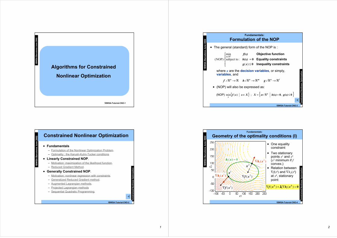
Algorithms for Constrained
Nonlinear Optimization
1BW
SA
Bar
celo
na
Jun
e 20
02
Co
nst
rain
ed
No
nlin
ear
Op
tim
izat
ion
1BWSA-Tutorial-CNO-2
Constrained Nonlinear Optimization
• Fundamentals– Formulation of the Nonlinear Optimization Problem.
– Optimality : the Karush-Kuhn-Tucker conditions
• Linearly Constrained NOP.– Motivation: maximization of the likelihood function.
– Reduced Gradient Method.
• Generally Constrained NOP.– Motivation: nonlinear regression with constraints.
– Generalized Reduced Gradient method.
– Augmented Lagrangian methods.
– Projected Lagrangian methods
– Sequential Quadratic Programming.
2
1BW
SA
Bar
celo
na
Jun
e 20
02
Co
nst
rain
ed
No
nlin
ear
Op
tim
izat
ion
1BWSA-Tutorial-CNO-3
Fundamentals:
Formulation of the NOP
• The general (standard) form of the NOP is :
≤=
ℜ∈
sconstraint Inequality
sconstraint Equality
function Objective
0
0
)(
:subject to
min
)NOP(
xg
h(x)
f(x)nx
where x are the decision variables, or simply,variables, and
lnmnn :g :h :f ℜ→ℜℜ→ℜℜ→ℜ
• (NOP) will also be expressed as:
, ; )(min 00 ≤=ℜ∈=∈ g(x)h(x)xXXxxf n
x(NOP)
1BW
SA
Bar
celo
na
Jun
e 20
02
Co
nst
rain
ed
No
nlin
ear
Op
tim
izat
ion
1BWSA-Tutorial-CNO-4
Fundamentals:
Geometry of the optimality conditions (I)
• Two stationarypoints x1 and x2
(x2 minimum if fconvex.)
)( 1xf∇
)( 21 xh∇
)( 2xf∇)( 11 xh∇
0)(1 =xh
• One equalityconstraint
1x
2x • Relation between∇f(xk) and ∇h1(xk)at xk, stationarypoint:
0=∇+∇ )()( 11kk xhxf λλλλ
3
1BW
SA
Bar
celo
na
Jun
e 20
02
Co
nst
rain
ed
No
nlin
ear
Op
tim
izat
ion
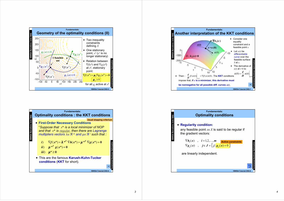
1BWSA-Tutorial-CNO-5
Fundamentals:
Geometry of the optimality conditions (II)
• One stationarypoint, x2 (x1 is nolonger stationary)
)( 1xf∇
)( 21 xg∇
)( 2xf∇)( 12 xg∇
• Relation between∇f(xk) and ∇gj(xk)at xk, stationarypoint:
0)(1 ≤xg
• Two inequalityconstraintsdefining X
0)(2 ≤xg
X feasibleset
0
)()(
≥
=∇+∇
j
kjj
k xgxf
µµµµµµµµ 0
for all gj active at xk
1x
2x
1BW
SA
Bar
celo
na
Jun
e 20
02
Co
nst
rain
ed
No
nlin
ear
Op
tim
izat
ion
1BWSA-Tutorial-CNO-6
Usual stopping criterium
Fundamentals:
Optimality conditions : the KKT conditions
• First-Order Necessary Conditions“Suppose that x* is a local minimizer of NOPand that x* is regular, then there are Lagrangemultipliers vectors λ∈ℜ m and µ∈ℜ l such that :
0
0
0
≥=
=∇+∇+∇
*)
*)(*)
*)(**)(**)()
µµµµµµµµ
µµµµλλλλ
iii
xgii
xgxhxfiT
TT
• This are the famous Karush-Kuhn-Tuckerconditions (KKT for short).
4
1BW
SA
Bar
celo
na
Jun
e 20
02
Co
nst
rain
ed
No
nlin
ear
Op
tim
izat
ion
1BWSA-Tutorial-CNO-7
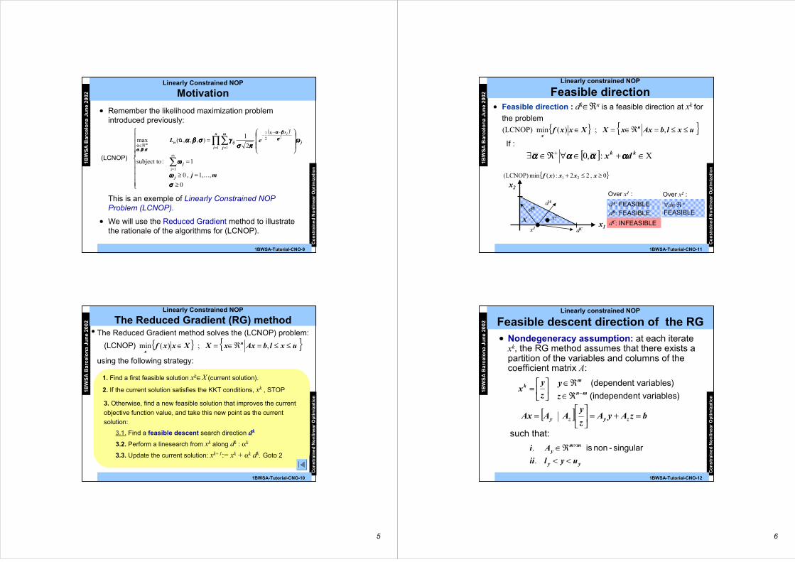
Fundamentals:
Another interpretation of the KKT conditions
x
∇∇∇∇h1(x )
S : h1(x)=0)0(x&
0
)()0(=
=t
txdt
dx&
• The derivative ofx(t) at t=0 is:
x(t)
• Let x(t) bedifferentiablecurve over thefeasible surfaceS at x.
=x (0)
• Consider oneequalityconstraint and afeasible point x
• Then : . The KKT conditions
impose that, if x is a minimizer, this derivative must
be nonnegative for all possible diff. curves x(t).
)0()())((0
xxftxfdt
d
t
&∇==
1BW
SA
Bar
celo
na
Jun
e 20
02
Co
nst
rain
ed
No
nlin
ear
Op
tim
izat
ion
1BWSA-Tutorial-CNO-8
Active constraints
0)(|,)(
,,2,1,)(
==∈∇=∇
xgjJjxg
mixh
jj
i K
Fundamentals:
Optimality conditions
• Regularity condition:
any feasible point x∈X is said to be regular ifthe gradient vectors:
are linearly independent.
5
1BW
SA
Bar
celo
na
Jun
e 20
02
Co
nst
rain
ed
No
nlin
ear
Op
tim
izat
ion
1BWSA-Tutorial-CNO-9
Linearly Constrained NOP
Motivation
• Remember the likelihood maximization problemintroduced previously:
( )
≥=≥
=
=
∑
∏∑
=
−−−
= =ℜ∈
0
,,1,0
1: subject to
2
1),,,(max
m
1j
2
1
1 1,,
2
2
σσσσωωωω
ωωωω
ωωωωππππσσσσ
γγγγσσσσββββαααα σσσσββββαααα
σσσσββββαααα
mj
eL
j
j
j
syn
i
m
jijn
ji
m
K
ùù
(LCNOP)
• We will use the Reduced Gradient method to illustratethe rationale of the algorithms for (LCNOP).
This is an exemple of Linearly Constrained NOPProblem (LCNOP).
1BW
SA
Bar
celo
na
Jun
e 20
02
Co
nst
rain
ed
No
nlin
ear
Op
tim
izat
ion
1BWSA-Tutorial-CNO-10
1. Find a first feasible solution xk∈X (current solution).
2. If the current solution satisfies the KKT conditions, xk , STOP
3. Otherwise, find a new feasible solution that improves the current
objective function value, and take this new point as the current
solution:
3.1. Find a feasible descent search direction dk
3.2. Perform a linesearch from xk along dk : αk
3.3. Update the current solution: xk+1:= xk + αk dk. Goto 2
Linearly Constrained NOP
The Reduced Gradient (RG) method• The Reduced Gradient method solves the (LCNOP) problem:
uxlbAxxXXxxf n
x≤≤=ℜ∈=∈ , ; )(min (LCNOP)
using the following strategy:
6
1BW
SA
Bar
celo
na
Jun
e 20
02
Co
nst
rain
ed
No
nlin
ear
Op
tim
izat
ion
1BWSA-Tutorial-CNO-11
0,22:)(min (LCNOP) 21 ≥≤+ xxxxf
x1
x2
X
Linearly constrained NOP
Feasible direction• Feasible direction : dk∈ℜn is a feasible direction at xk for
the problem
dB
dC
dA dA: FEASIBLE
dB: FEASIBLE
dC: INFEASIBLEx1
Over x1 :
x2
Over x2 :
∀d∈ℜ n
FEASIBLE
uxlbAxxXXxxf n
x≤≤=ℜ∈=∈ , ; )(min (LCNOP)
[ ] X:,0 ∈+∈∀ℜ∈∃ + kk dx ααααααααααααααααIf :
1BW
SA
Bar
celo
na
Jun
e 20
02
Co
nst
rain
ed
No
nlin
ear
Op
tim
izat
ion
1BWSA-Tutorial-CNO-12
Linearly constrained NOP
Feasible descent direction of the RG• Nondegeneracy assumption: at each iterate
xk, the RG method assumes that there exists apartition of the variables and columns of thecoefficient matrix A:
variables) nt(independe
variables) (dependentmn
mk
z
y
z
yx −ℜ∈
ℜ∈
=
such that:
[ ] bzAyAz
yAAAx zyzy =+=
=
yy
mmy
uylii
Ai
<<ℜ∈ ×
.
. singular-non is
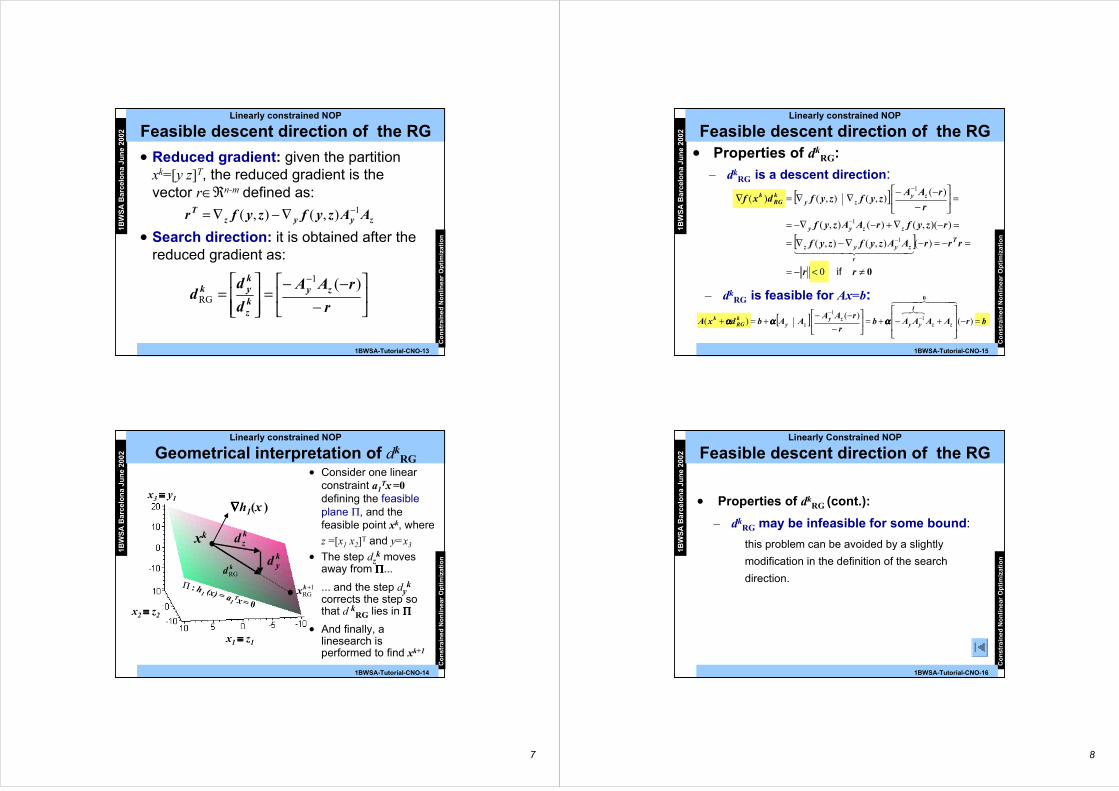
7
1BW
SA
Bar
celo
na
Jun
e 20
02
Co
nst
rain
ed
No
nlin
ear
Op
tim
izat
ion
1BWSA-Tutorial-CNO-13
Linearly constrained NOP
Feasible descent direction of the RG
• Reduced gradient: given the partitionxk=[y z]T, the reduced gradient is thevector r∈ℜn-m defined as:
zyyzT AAzyfzyfr 1),(),( −∇−∇=
• Search direction: it is obtained after thereduced gradient as:
−
−−=
=
−
r
rAA
d
dd zy
kz
kyk )(1
RG
1BW
SA
Bar
celo
na
Jun
e 20
02
Co
nst
rain
ed
No
nlin
ear
Op
tim
izat
ion
1BWSA-Tutorial-CNO-14
xk
∇∇∇∇h1(x )
x1 ≡≡≡≡ z1
x2 ≡≡≡≡ z2
x3 ≡≡≡≡ y1
Π : h1 (x) = a
1Tx = 0
Linearly constrained NOP
Geometrical interpretation of dkRG
kdRG
• Consider one linearconstraint a1
Tx =0defining the feasibleplane Π, and thefeasible point xk, where
z =[x1 x2]T and y=x3
kyd
... and the step dyk
corrects the step sothat d kRG lies in ΠΠΠΠ
1RG+kx
• And finally, alinesearch isperformed to find xk+1
kzd
• The step dzk moves
away from ΠΠΠΠ...
8
1BW
SA
Bar
celo
na
Jun
e 20
02
Co
nst
rain
ed
No
nlin
ear
Op
tim
izat
ion
1BWSA-Tutorial-CNO-15
[ ] brAAAAbr
rAAAAbdxA zz
I
yyzy
zykRG
k =−
+−+=
−
−−+=+ −−
)()(
)( 11
444 8444 76876
0
αααααααααααα
Linearly constrained NOP
Feasible descent direction of the RG• Properties of dk
RG:
– dkRG is a descent direction:
[ ]
[ ]0≠<−=
=−=−∇−∇=
=−∇+−−∇=
=
−
−−∇∇=∇
−
−
−
rr
rrrAAzyfzyf
rzyfrAAzyf
r
rAAzyfzyfdxf
T
r
zyyz
zzyy
zyzy
kRG
k
if0
)(),(),(
))(,()(),(
)(),(),()(
1
1
1
44444 344444 21
– dkRG is feasible for Ax=b:
1BW
SA
Bar
celo
na
Jun
e 20
02
Co
nst
rain
ed
No
nlin
ear
Op
tim
izat
ion
1BWSA-Tutorial-CNO-16
Linearly Constrained NOP
Feasible descent direction of the RG
• Properties of dkRG (cont.):
– dkRG may be infeasible for some bound:
this problem can be avoided by a slightly
modification in the definition of the search
direction.
9
1BW
SA
Bar
celo
na
Jun
e 20
02
Co
nst
rain
ed
No
nlin
ear
Op
tim
izat
ion
1BWSA-Tutorial-CNO-17
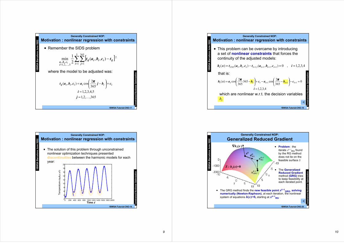
Generally Constrained NOP:
Motivation : nonlinear regression with constraints
• Remember the SIDS problem
[ ]∑∑= ==
−5
1
365
1
2
5,,2,1,,
),,(2
1min
i jijiiiij
icba
tcbatiiiK
where the model to be adjusted was:
365,,2,1
5,4,3,2,1
365
2cos),,(
K==
+
−=
j
i
cbjacbat iiiiiiij
ππππ
1BW
SA
Bar
celo
na
Jun
e 20
02
Co
nst
rain
ed
No
nlin
ear
Op
tim
izat
ion
1BWSA-Tutorial-CNO-18
Generally Constrained NOP:
Motivation : nonlinear regression with constraints
• The solution of this problem through unconstrainednonlinear optimization techniques presenteddiscontinuities between the harmonic models for eachyear:
0 200 400 600 800 1000 1200 1400 1600 1800 20002
4
6
8
10
12
14
16
18
20
Time d
Te
mpe
ratu
re t
(a,b
,c;
d )
10
1BW
SA
Bar
celo
na
Jun
e 20
02
Co
nst
rain
ed
No
nlin
ear
Op
tim
izat
ion
1BWSA-Tutorial-CNO-19
which are nonlinear w.r.t. the decision variablesbi
Generally Constrained NOP:
Motivation : nonlinear regression with constraints
• This problem can be overcame by introducinga set of nonlinear constraints that forces thecontinuity of the adjusted models:
4,3,2,1,0),,(),,()( 1111,1365 ==−= ++++ icbatcbatxh iiiiiiiii
4,3,2,1
0365
2cos365
365
2cos)( 111
=
=−
−−+
−= +++
i
cbacbaxh iiiiiii
ππππππππ
that is:
1BW
SA
Bar
celo
na
Jun
e 20
02
Co
nst
rain
ed
No
nlin
ear
Op
tim
izat
ion
1BWSA-Tutorial-CNO-20
xk
∇∇∇∇h1(x )
Generally Constrained NOP:
Generalized Reduced Gradient
S : h1(x)=0
• Problem : theiterate xk+1
RG foundby the RG methoddoes not lie on thefeasible surface S
• The GeneralizedReduced Gradientmethod (GRG) triesto keep feasibility ateach iterated point.
kdRG1
RG+kx
1GRG+kx
• The GRG method finds the new feasible point xk+1GRG, solving
numerically (Newton-Raphson), at each iteration, the nonlinearsystem of equations h(x)=0, starting at xk+1
RG .
11
1BW
SA
Bar
celo
na
Jun
e 20
02
Co
nst
rain
ed
No
nlin
ear
Op
tim
izat
ion
1BWSA-Tutorial-CNO-21
Generally Constrained NOP:
Augmented Lagrangian Methods (I)
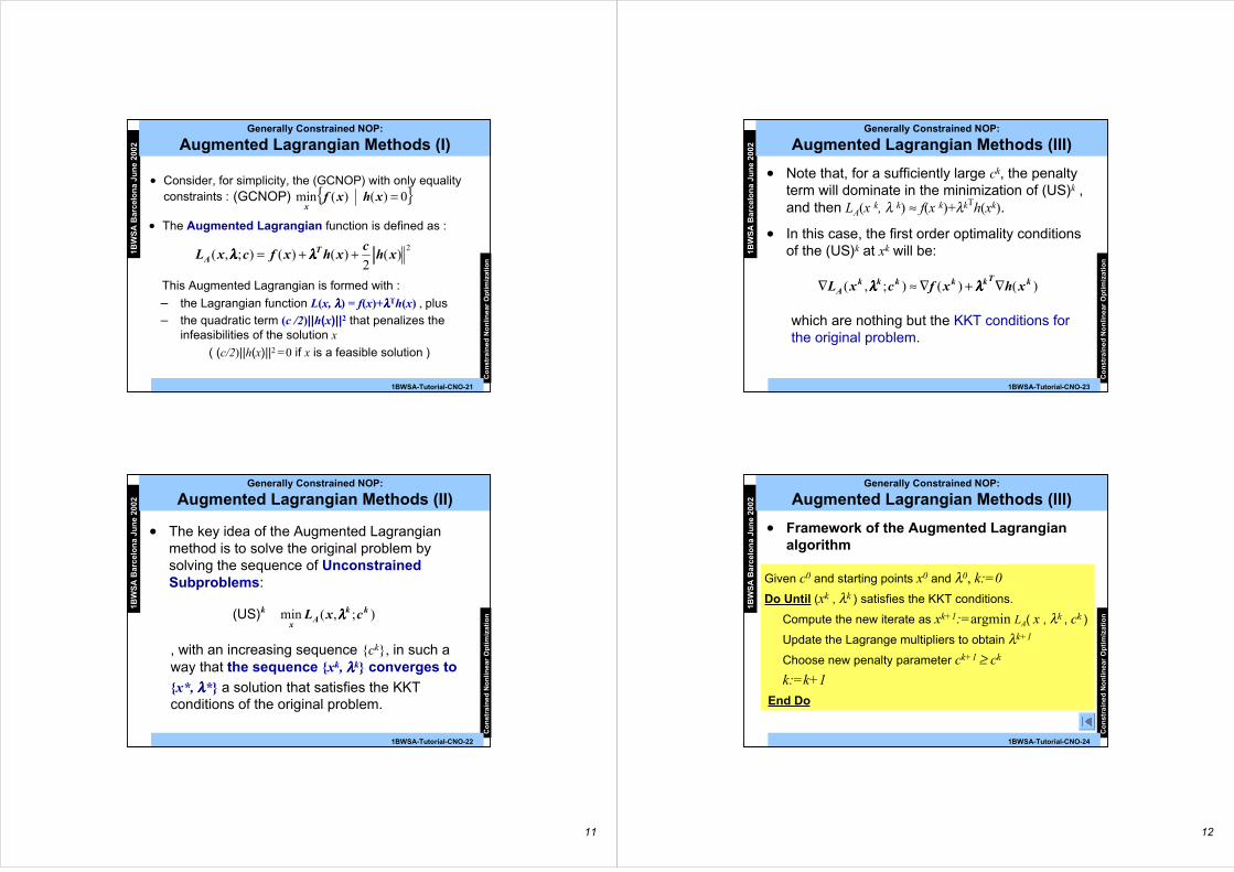
• Consider, for simplicity, the (GCNOP) with only equalityconstraints : 0)( )(min =xhxf
x(GCNOP)
• The Augmented Lagrangian function is defined as :
2)(
2)()();,( xh
cxhxfcxL T
A ++= λλλλλλλλ
This Augmented Lagrangian is formed with :
– the Lagrangian function L(x, λλλλ) = f(x)+λλλλTh(x) , plus
– the quadratic term (c /2)||h(x)||2 that penalizes theinfeasibilities of the solution x
( (c/2)||h(x)||2 =0 if x is a feasible solution )
1BW
SA
Bar
celo
na
Jun
e 20
02
Co
nst
rain
ed
No
nlin
ear
Op
tim
izat
ion
1BWSA-Tutorial-CNO-22
Generally Constrained NOP:
Augmented Lagrangian Methods (II)
• The key idea of the Augmented Lagrangianmethod is to solve the original problem bysolving the sequence of UnconstrainedSubproblems:
);,(min kkA
x
k cxL λλλλ(US)
, with an increasing sequence ck, in such away that the sequence xk, λλλλk converges to
x*, λλλλ* a solution that satisfies the KKTconditions of the original problem.
12
1BW
SA
Bar
celo
na
Jun
e 20
02
Co
nst
rain
ed
No
nlin
ear
Op
tim
izat
ion
1BWSA-Tutorial-CNO-23
Generally Constrained NOP:
Augmented Lagrangian Methods (III)
• In this case, the first order optimality conditionsof the (US)k at xk will be:
)()();,( kTkkkkkA xhxfcxL ∇+∇≈∇ λλλλλλλλ
which are nothing but the KKT conditions forthe original problem.
• Note that, for a sufficiently large ck, the penaltyterm will dominate in the minimization of (US)k ,and then LA(x k, λ k) ≈ f(x k)+λkTh(xk).
1BW
SA
Bar
celo
na
Jun
e 20
02
Co
nst
rain
ed
No
nlin
ear
Op
tim
izat
ion
1BWSA-Tutorial-CNO-24
Generally Constrained NOP:
Augmented Lagrangian Methods (III)
• Framework of the Augmented Lagrangianalgorithm
Given c0 and starting points x0 and λ0, k:=0
Do Until (xk , λk ) satisfies the KKT conditions.
Compute the new iterate as xk+1:=argmin LA( x , λk , ck )
Update the Lagrange multipliers to obtain λk+1
Choose new penalty parameter ck+1 ≥ ck
k:=k+1
End Do

13
1BW
SA
Bar
celo
na
Jun
e 20
02
Co
nst
rain
ed
No
nlin
ear
Op
tim
izat
ion
1BWSA-Tutorial-CNO-25
where the linear constraints comes from the Taylor’sseries expansion of h(x) around a given point xk.
Generally Constrained NOP:
Projected Lagrangian Methods (I)
• Consider, again, the (GCNOP) with only equality
constraints : 0=)( )(min xhxfx
(GCNOP)
• Projected Lagrangian methods solve the originalproblem by solving the sequence of LinearlyConstrained Subproblems:
=+−∇ 0)())((: tosubj.
);,(minkkk
kkP
xk
xhxxxh
cxL λλλλ(LCS)
1BW
SA
Bar
celo
na
Jun
e 20
02
Co
nst
rain
ed
No
nlin
ear
Op
tim
izat
ion
1BWSA-Tutorial-CNO-26
Generally Constrained NOP:
Projected Lagrangian Methods (II)
• The most effective expression of the objective functionof subproblems (LCS)k is the Modified AugmentedLagrangian:
2)(
2)()(),,;( xh
cxhxfcxxL kkTkkkk
P ++= λλλλλλλλ
that resembles the Augmented Lagrangian function,excepts that the expression of the nonlinearconstraints h(x) has been substituted by hk(x), definedas:
[ ]4444 34444 21
)(
)())(()()(kxxh
kkkk xhxxxhxhxh
around of ionapproximat Linear
+−∇−=
• Near the solution ( (xk , λk) ≈ (x* , λ* ) ) the methodpresents quadratic order of convergence if c=0.
14
1BW
SA
Bar
celo
na
Jun
e 20
02
Co
nst
rain
ed
No
nlin
ear
Op
tim
izat
ion
1BWSA-Tutorial-CNO-27
Generally Constrained NOP:
Projected Lagrangian Methods (III)
• Projected Lagrangian algorithm
Given c0 and starting points x0 and λ0, k:=0
Do Until (xk , λk ) satisfies the KKT conditions.
Solve (LCS) k to obtain xk+1
Take λk+1 as the Lag. mult. at the opt. sol. of (LCS) k
If (xk , λk) ≈ (x* , λ*) then set ck+1 = 0
Else choose ck+1 ≥ ck
k:=k+1
End Do
1BW
SA
Bar
celo
na
Jun
e 20
02
Co
nst
rain
ed
No
nlin
ear
Op
tim
izat
ion
1BWSA-Tutorial-CNO-28
Generally Constrained NOP:
Sequential Quadratic Programming (I)
• Consider, the problem : 0=)( )(min xhxfx
(GCNOP)
where the matrix Wk ∈ ℜn×n denotes the Hessian of
the Lagrangian function at (xk, λk ) :
∑=
∇+∇=∇=m
j
kkj
kkkxx
k xhxfxLW1
222 )()(),( λλλλλλλλ
• Sequential Quadratic Programming solves theoriginal problem by solving the sequence of QuadraticLinearly Constrained Subproblems:
( ) ( ) ( )
=+−∇
−∇+−−
0)())((: tosubj.
)(2
1min
kkk
kkkkTk
xk
xhxxxh
xxxfxxWxx(QLCS)

15
1BW
SA
Bar
celo
na
Jun
e 20
02
Co
nst
rain
ed
No
nlin
ear
Op
tim
izat
ion
1BWSA-Tutorial-CNO-29
Generally Constrained NOP:
Sequential Quadratic Programming (II)
• Framework of the Sequential QuadraticProgramming
Given starting points x0 and λ0, k:=0
Do Until (xk , λk) satisfies the KKT conditions.
Solve (QLCS) k to obtain xk+1.
Take λk+1 as the Lag. mult. at the opt. sol. of (QLCS) k
k:=k+1
End Do
1BW
SA
Bar
celo
na
Jun
e 20
02
Co
nst
rain
ed
No
nlin
ear
Op
tim
izat
ion
1BWSA-Tutorial-CNO-30
Generally Constrained NOP:
SQP and Projected Lagrangian
• The strategy of the SQP is similar to the one used in
the Projected Lagrangian methods:
– Advantages of SQP: it is easier to optimize the quadratic
subproblem (QLCS)k than the general (LCS)k, due to the
existence of specialised quadratic programming techniques.
– Disadvantages of SQP: the computation of the quadratic
objective function needs the second derivatives (or its
numerical approximation) of the objective function f(x) and
constraints h(x).
• Both methods can be proved to converge quadratically
near the solution.
1
1BWSA-Tutorial-Solvers-1
1BW
SA
Ba
rcel
on
a J
un
e 20
02
Solvers for Nonlinear
Optimization
1BW
SA
Bar
celo
na
Jun
e 20
02
So
lver
s fo
r N
on
lin
ear
Op
tim
izat
ion
1BWSA-Tutorial-Solvers-2
Solvers for nonlinear optimization
• Optimization libraries.– Solving the SIDS problem with the NAG
Library Without smoothness constraints. With smoothness constraints.
• Modeling languages.– Maximization of the constrained likelihood
function with AMPL
2
1BW
SA
Bar
celo
na
Jun
e 20
02
So
lver
s fo
r N
on
lin
ear
Op
tim
izat
ion
1BWSA-Tutorial-Solvers-3
Optimization libraries:
Description
• Optimization libraries provides subroutines that can be
called from the user’s own code (mainly in FORTRAN, C
or MATLAB).
• In order to solve a problem with an optimization library, the
user must provide:
• The data structure with the relevant information about the problem
( matrix A in the (LCNOP), lower and upper bounds, etc.)
• Subroutines that, given a vector xk, returns all the information
needed by the algorithm. This information could be:
At least f(xk) and the constraints value h(xk) and g(xk).
Usually the gradients ∇∇∇∇f(xk) and Jacobians ∇∇∇∇h(xk) and ∇∇∇∇g(xk).
Rarely, the Hessians ∇∇∇∇2f(xk), ∇∇∇∇2h(xk) and ∇∇∇∇2g(xk).
1BW
SA
Bar
celo
na
Jun
e 20
02
So
lver
s fo
r N
on
lin
ear
Op
tim
izat
ion
1BWSA-Tutorial-Solvers-4
Optimization libraries:
Optimization libraries
• Some of most outstanding optimization libraries are:
– For Unconstrained Optimization:
The optimization subroutines in the NAG and HARWELL libraries.
– For Constrained Optimization:
GRG, CONOP: Generalized Reduced Gradient.
LANCELOT : Augmented Lagrangians.
MINOS : Projected Lagrangians.
SNOPT: Sequential Quadratic Programming.
• But, if you really are interested in knowing all the
available optimization software, visit the NEOS Guide at
www-fp.mcs.anl.gov/otc/Guide/ (a really impressive site
in optimization!!)

3
1BW
SA
Bar
celo
na
Jun
e 20
02
So
lver
s fo
r N
on
lin
ear
Op
tim
izat
ion
1BWSA-Tutorial-Solvers-5
Optimization libraries:
Solving the SIDS problem with the NAG libraries
• Subroutines for the unconstrained SIDS problem :– E04JAF : Quasi-Newton, using function values only.
– E04GCF: Gauss-Newton, using function values andfirst derivatives.
• Subroutines for the constrained SIDS problem:– E04UCF: Sequential Quadratic Programming, using
function values and first derivatives.
• We will see how to solve the SIDS problem callingthese subroutines from MATLAB.
1BW
SA
Bar
celo
na
Jun
e 20
02
So
lver
s fo
r N
on
lin
ear
Op
tim
izat
ion
1BWSA-Tutorial-Solvers-6
Optimization libraries:
Subroutine E04JAF (QN method)
• Main program: file SIDS_e04jaf.m
% Solving the SIDS problem with the NAG Foundation Library
% Routine E04jaf : Quasi-Newton method using function values only
'Example program for the NAG Foundation Library Routine e04jaf'
SIDS_t; % Here the observed data t_ij is loaded
x=zeros(15,1); % Initial point
time=cputime; % To know the total execution time.
[xQN,f] = e04jaf(x); % This is the call to the subroutine
Optimal_Objective_Function=f % We print f(x*)...
At_the_Point_X=xQN % ... the optimal solution x*...
time = cputime-time % ... and the execution time
4
1BW
SA
Bar
celo
na
Jun
e 20
02
So
lver
s fo
r N
on
lin
ear
Op
tim
izat
ion
1BWSA-Tutorial-Solvers-7
Optimization libraries:
Subroutine E04JAF (QN method)• User’s subroutines: computation of f(xk) file funct1.m
% Objective function for the SIDS problemfunction [fc] = funct1(n,xc)global obs;fc=0;ww=(2*pi)/365;for i=0:4 aux = 3*i; a = xc(1+aux); b = xc(2+aux); c = xc(3+aux); aux2 = 365*i; for j=1:365 calc=a*cos(ww*j-b)+c; fc=fc+(calc-obs(j+aux2))^2; endendfc=fc/2;
1BW
SA
Bar
celo
na
Jun
e 20
02
So
lver
s fo
r N
on
lin
ear
Op
tim
izat
ion
1BWSA-Tutorial-Solvers-8
Optimization libraries:
Subroutine E04JAF (QN method)• Output:
» sids_e04jafe
ans =
Example program for the NAGFoundation Library Routine
e04jaf
Optimal_Objective_Function =
6.8569e+003
» sids_e04jafe
ans =
Example program for the NAGFoundation Library Routine
e04jaf
Optimal_Objective_Function =
6.8569e+003
At_the_Point_X =
-6.9691
0.4920 9.7255
-6.0992 6.7046
11.4230 -6.4842
0.3844 11.2986
-6.7013
-5.8949 12.0551
-6.9693 6.8088
12.0827
time = 18.8900
At_the_Point_X =
-6.9691
0.4920 9.7255
-6.0992 6.7046
11.4230 -6.4842
0.3844 11.2986
-6.7013
-5.8949 12.0551
-6.9693 6.8088
12.0827
time = 18.8900
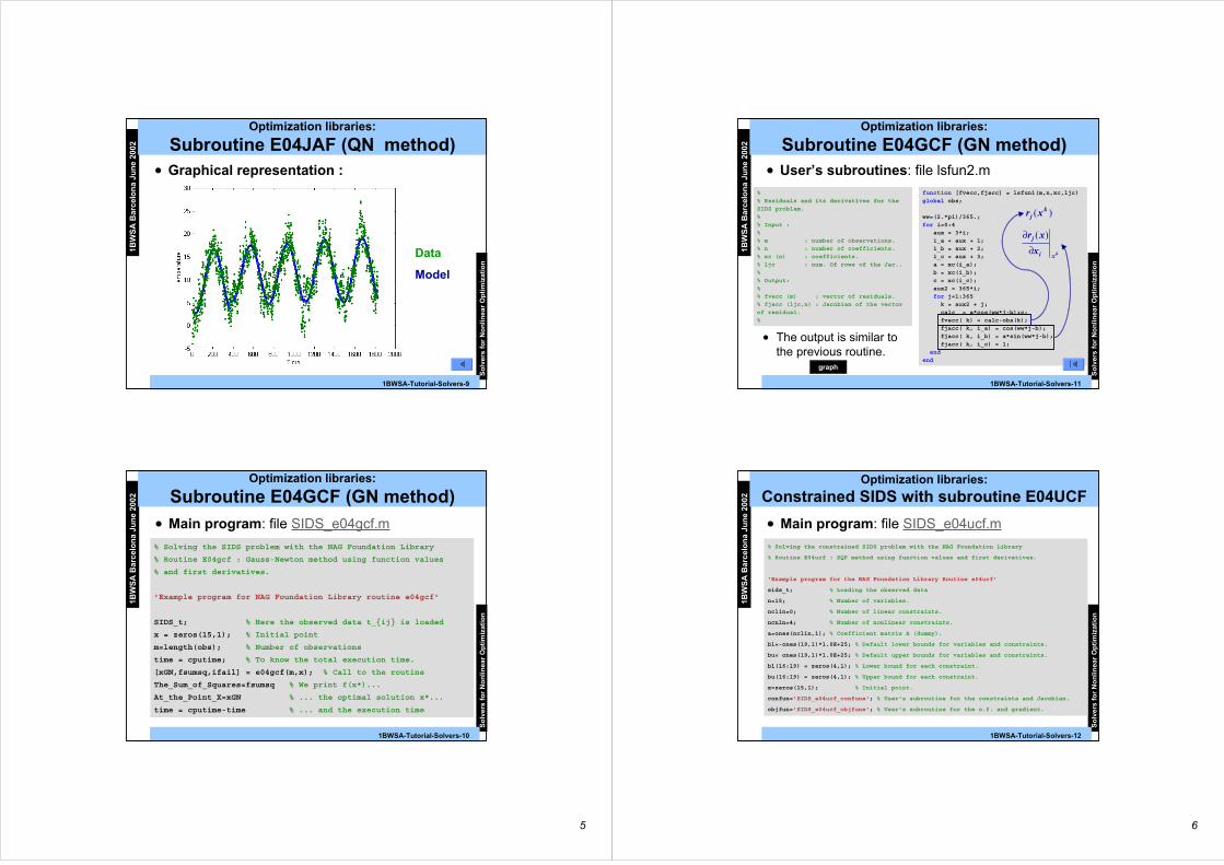
5
1BW
SA
Bar
celo
na
Jun
e 20
02
So
lver
s fo
r N
on
lin
ear
Op
tim
izat
ion
1BWSA-Tutorial-Solvers-9
Optimization libraries:
Subroutine E04JAF (QN method)
Data
Model
• Graphical representation :
1BW
SA
Bar
celo
na
Jun
e 20
02
So
lver
s fo
r N
on
lin
ear
Op
tim
izat
ion
1BWSA-Tutorial-Solvers-10
Optimization libraries:
Subroutine E04GCF (GN method)
• Main program: file SIDS_e04gcf.m
% Solving the SIDS problem with the NAG Foundation Library
% Routine E04gcf : Gauss-Newton method using function values
% and first derivatives.
'Example program for NAG Foundation Library routine e04gcf'
SIDS_t; % Here the observed data t_ij is loaded
x = zeros(15,1); % Initial point
m=length(obs); % Number of observations
time = cputime; % To know the total execution time.
[xGN,fsumsq,ifail] = e04gcf(m,x); % Call to the routine
The_Sum_of_Squares=fsumsq % We print f(x*)...
At_the_Point_X=xGN % ... the optimal solution x*...
time = cputime-time % ... and the execution time
6
1BW
SA
Bar
celo
na
Jun
e 20
02
So
lver
s fo
r N
on
lin
ear
Op
tim
izat
ion
1BWSA-Tutorial-Solvers-11
Optimization libraries:
Subroutine E04GCF (GN method)• User’s subroutines: file lsfun2.m
%
% Residuals and its derivatives for the
SIDS problem.
%
% Input :
%
% m : number of observations.
% n : number of coefficients.
% xc (n) : coefficients.
% ljc : num. Of rows of the Jac..
%
% Output:
%
% fvecc (m) : vector of residuals.
% fjacc (ljc,n) : Jacobian of the vector
of residual.
%
function [fvecc,fjacc] = lsfun1(m,n,xc,ljc)
global obs;
ww=(2.*pi)/365.;
for i=0:4
aux = 3*i;
i_a = aux + 1;
i_b = aux + 2;
i_c = aux + 3;
a = xc(i_a);
b = xc(i_b);
c = xc(i_c);
aux2 = 365*i;
for j=1:365
k = aux2 + j;
calc = a*cos(ww*j-b)+c;
fvecc( k) = calc-obs(k);
fjacc( k, i_a) = cos(ww*j-b);
fjacc( k, i_b) = a*sin(ww*j-b);
fjacc( k, i_c) = 1;
end
end
• The output is similar tothe previous routine.
)( kj xr
kxi
j
x
xr
∂∂ )(
graph
1BW
SA
Bar
celo
na
Jun
e 20
02
So
lver
s fo
r N
on
lin
ear
Op
tim
izat
ion
1BWSA-Tutorial-Solvers-12
Optimization libraries:
Constrained SIDS with subroutine E04UCF
• Main program: file SIDS_e04ucf.m
% Solving the constrained SIDS problem with the NAG Foundation Library
% Routine E04ucf : SQP method using function values and first derivatives.
'Example program for the NAG Foundation Library Routine e04ucf'
sids_t; % Loading the observed data
n=15; % Number of variables.
nclin=0; % Number of linear constraints.
ncnln=4; % Number of nonlinear constraints.
a=ones(nclin,1); % Coefficient matrix A (dummy).
bl=-ones(19,1)*1.0E+25; % Default lower bounds for variables and constraints.
bu= ones(19,1)*1.0E+25; % Default upper bounds for variables and constraints.
bl(16:19) = zeros(4,1); % Lower bound for each constraint.
bu(16:19) = zeros(4,1); % Upper bound for each constraint.
x=zeros(15,1); % Initial point.
confun='SIDS_e04ucf_confune'; % User's subroutine for the constraints and Jacobian.
objfun='SIDS_e04ucf_objfune'; % User's subroutine for the o.f. and gradient.
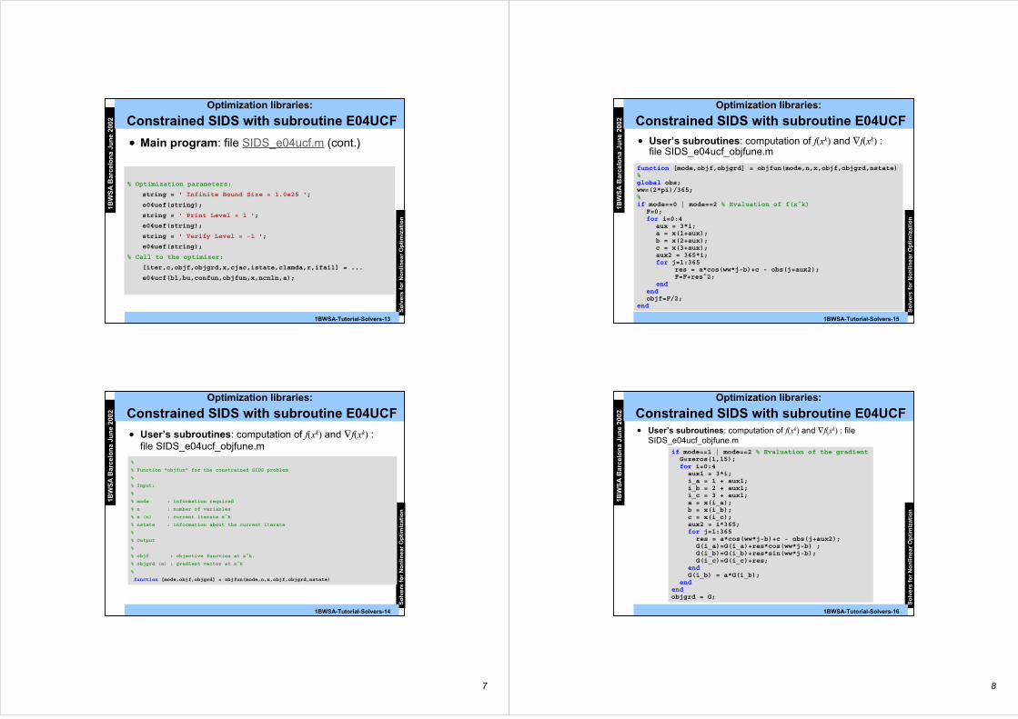
7
1BW
SA
Bar
celo
na
Jun
e 20
02
So
lver
s fo
r N
on
lin
ear
Op
tim
izat
ion
1BWSA-Tutorial-Solvers-13
Optimization libraries:
Constrained SIDS with subroutine E04UCF
• Main program: file SIDS_e04ucf.m (cont.)
% Optimization parameters:
string = ' Infinite Bound Size = 1.0e25 ';
e04uef(string);
string = ' Print Level = 1 ';
e04uef(string);
string = ' Verify Level = -1 ';
e04uef(string);
% Call to the optimizer:
[iter,c,objf,objgrd,x,cjac,istate,clamda,r,ifail] = ...
e04ucf(bl,bu,confun,objfun,x,ncnln,a);
1BW
SA
Bar
celo
na
Jun
e 20
02
So
lver
s fo
r N
on
lin
ear
Op
tim
izat
ion
1BWSA-Tutorial-Solvers-14
Optimization libraries:
Constrained SIDS with subroutine E04UCF
• User’s subroutines: computation of f(xk) and ∇f(xk) :file SIDS_e04ucf_objfune.m
%
% Function "objfun" for the constrained SIDS problem
%
% Input:
%
% mode : information required
% n : number of variables
% x (n) : current iterate x^k
% nstate : information about the current iterate
%
% Output
%
% objf : objective function at x^k.
% objgrd (n) : gradient vector at x^k
%
function [mode,objf,objgrd] = objfun(mode,n,x,objf,objgrd,nstate)
8
1BW
SA
Bar
celo
na
Jun
e 20
02
So
lver
s fo
r N
on
lin
ear
Op
tim
izat
ion
1BWSA-Tutorial-Solvers-15
Optimization libraries:
Constrained SIDS with subroutine E04UCF
• User’s subroutines: computation of f(xk) and ∇f(xk) :file SIDS_e04ucf_objfune.m
function [mode,objf,objgrd] = objfun(mode,n,x,objf,objgrd,nstate)%global obs;ww=(2*pi)/365;%if mode==0 | mode==2 % Evaluation of f(x^k)
F=0;for i=0:4
aux = 3*i; a = x(1+aux); b = x(2+aux); c = x(3+aux); aux2 = 365*i; for j=1:365 res = a*cos(ww*j-b)+c - obs(j+aux2); F=F+res^2; end
endobjf=F/2;
end
1BW
SA
Bar
celo
na
Jun
e 20
02
So
lver
s fo
r N
on
lin
ear
Op
tim
izat
ion
1BWSA-Tutorial-Solvers-16
Optimization libraries:
Constrained SIDS with subroutine E04UCF• User’s subroutines: computation of f(xk) and ∇f(xk) : file
SIDS_e04ucf_objfune.mif mode==1 | mode==2 % Evaluation of the gradient
G=zeros(1,15);for i=0:4
aux1 = 3*i; i_a = 1 + aux1; i_b = 2 + aux1; i_c = 3 + aux1; a = x(i_a); b = x(i_b); c = x(i_c); aux2 = i*365; for j=1:365 res = a*cos(ww*j-b)+c - obs(j+aux2); G(i_a)=G(i_a)+res*cos(ww*j-b) ; G(i_b)=G(i_b)+res*sin(ww*j-b); G(i_c)=G(i_c)+res; end G(i_b) = a*G(i_b);
endendobjgrd = G;
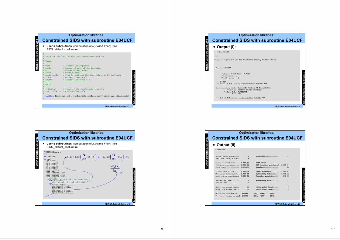
9
1BW
SA
Bar
celo
na
Jun
e 20
02
So
lver
s fo
r N
on
lin
ear
Op
tim
izat
ion
1BWSA-Tutorial-Solvers-17
Optimization libraries:
Constrained SIDS with subroutine E04UCF• User’s subroutines: computation of h(xk) and ∇h(xk) : file
SIDS_e04ucf_confune.m
%% Function "objfun" for the constrained SIDS problem%% Input:%% mode : information required% ncnln : number of rows of the Jacobian.% n : number of variables% nrows : max(1,ncnln)% needc(ncnln) : flag to indicate the constraints to be evaluated.% x (n) : current iterate x^k% nstate : information about x^k.%% Output%% c (ncnln) : value of the constraints over x^k% cjac (nrowj,n) : Jacobian over x^k% function [mode,c,cjac] = confun(mode,ncnln,n,nrowj,needc,x,c,cjac,nstate)%
1BW
SA
Bar
celo
na
Jun
e 20
02
So
lver
s fo
r N
on
lin
ear
Op
tim
izat
ion
1BWSA-Tutorial-Solvers-18
Optimization libraries:
Constrained SIDS with subroutine E04UCF• User’s subroutines: computation of h(xk) and ∇h(xk) : file
SIDS_e04ucf_confune.mif nstate==1 cjac=zeros(ncnln,n);end
ww = 2*pi/365;
for i=1:4 aux = 3*(i-1); a0 = x(aux+1); b0 = x(aux+2); c0 = x(aux+3); a1 = x(aux+4); b1 = x(aux+5); c1 = x(aux+6); aux0 = ww*365.; aux1 = ww; cos0 = cos(aux0 - b0); sin0 = sin(aux0 - b0); cos1 = cos(aux1 - b1); sin1 = sin(aux1 - b1);
if needc(i)>0 % Continuity of y(j,t) at the "i"-th connect point if mode==0 | mode==2 c(i) = a0*cos0 + c0 - ( a1*cos1 + c1); end if mode==1 | mode==2 cjac(i,aux+1) = cos0; cjac(i,aux+2) = a0*sin0; cjac(i,aux+3) = 1.; cjac(i,aux+4) = -cos1; cjac(i,aux+5) = -a1*sin1; cjac(i,aux+6) = -1.; end endend
111 365
2cos365
365
2cos)( +++ −
−−+
−= iiiiiii cbacbaxh
ππππππππ
kxj
i
x
xh
∂∂ )(
10
1BW
SA
Bar
celo
na
Jun
e 20
02
So
lver
s fo
r N
on
lin
ear
Op
tim
izat
ion
1BWSA-Tutorial-Solvers-19
Optimization libraries:
Constrained SIDS with subroutine E04UCF
• Output (I):» sids_e04ucfE
ans =
Example program for the NAG Foundation Library Routine e04ucf
Calls to E04UEF ---------------
Infinite Bound Size = 1.0e25 Print Level = 1 Verify Level = -1
*** E04UCF *** Start of NAG Library implementation details ***
Implementation title: Microsoft Windows NT Powerstation Precision: FORTRAN Double Precision Product Code: FLNTI17DI Mark: 17A
*** End of NAG Library implementation details ***
» sids_e04ucfE
ans =
Example program for the NAG Foundation Library Routine e04ucf
Calls to E04UEF ---------------
Infinite Bound Size = 1.0e25 Print Level = 1 Verify Level = -1
*** E04UCF *** Start of NAG Library implementation details ***
Implementation title: Microsoft Windows NT Powerstation Precision: FORTRAN Double Precision Product Code: FLNTI17DI Mark: 17A
*** End of NAG Library implementation details ***
1BW
SA
Bar
celo
na
Jun
e 20
02
So
lver
s fo
r N
on
lin
ear
Op
tim
izat
ion
1BWSA-Tutorial-Solvers-20
Optimization libraries:
Constrained SIDS with subroutine E04UCF
• Output (II) :Parameters
----------
Linear constraints..... 0 Variables.............. 15
Nonlinear constraints.. 4
Infinite bound size.... 1.00D+25 COLD start.............
Infinite step size..... 1.00D+25 EPS (machine precision) 1.11D-16
Step limit............. 2.00D+00 Hessian................ NO
Linear feasibility..... 1.05D-08 Crash tolerance........ 1.00D-02
Nonlinear feasibility.. 1.05D-08 Optimality tolerance... 3.26D-12
Line search tolerance.. 9.00D-01 Function precision..... 4.38D-15
Derivative level....... 3 Monitoring file........ -1
Verify level........... -1
Major iterations limit. 85 Major print level...... 1
Minor iterations limit. 57 Minor print level...... 0
Workspace provided is IWORK( 53), WORK( 954).
To solve problem we need IWORK( 53), WORK( 954).
Parameters
----------
Linear constraints..... 0 Variables.............. 15
Nonlinear constraints.. 4
Infinite bound size.... 1.00D+25 COLD start.............
Infinite step size..... 1.00D+25 EPS (machine precision) 1.11D-16
Step limit............. 2.00D+00 Hessian................ NO
Linear feasibility..... 1.05D-08 Crash tolerance........ 1.00D-02
Nonlinear feasibility.. 1.05D-08 Optimality tolerance... 3.26D-12
Line search tolerance.. 9.00D-01 Function precision..... 4.38D-15
Derivative level....... 3 Monitoring file........ -1
Verify level........... -1
Major iterations limit. 85 Major print level...... 1
Minor iterations limit. 57 Minor print level...... 0
Workspace provided is IWORK( 53), WORK( 954).
To solve problem we need IWORK( 53), WORK( 954).
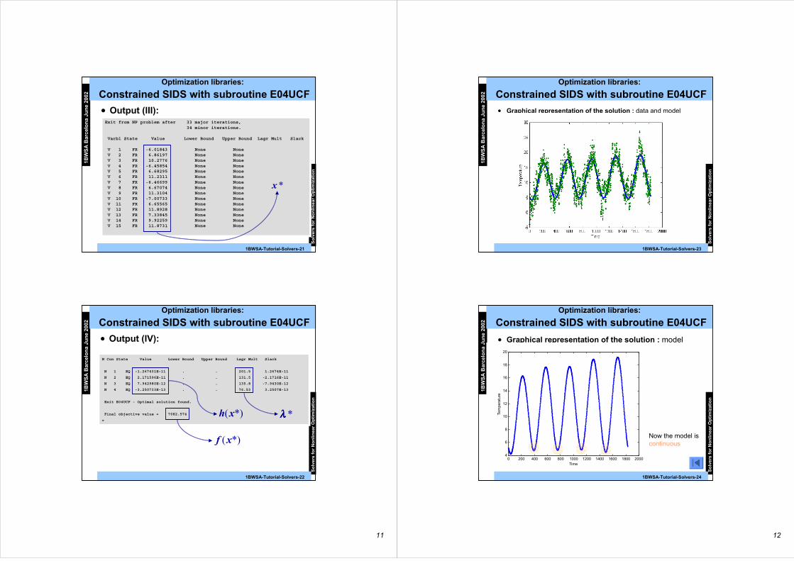
11
1BW
SA
Bar
celo
na
Jun
e 20
02
So
lver
s fo
r N
on
lin
ear
Op
tim
izat
ion
1BWSA-Tutorial-Solvers-21
Optimization libraries:
Constrained SIDS with subroutine E04UCF
• Output (III):Exit from NP problem after 33 major iterations, 34 minor iterations.
Varbl State Value Lower Bound Upper Bound Lagr Mult Slack
V 1 FR -6.01843 None None V 2 FR 6.86197 None None V 3 FR 10.2776 None None V 4 FR -6.45854 None None V 5 FR 6.68295 None None V 6 FR 11.2311 None None V 7 FR -6.46699 None None V 8 FR 6.67074 None None V 9 FR 11.3104 None None V 10 FR -7.00733 None None V 11 FR 6.65565 None None V 12 FR 11.8928 None None V 13 FR 7.33845 None None V 14 FR 9.92259 None None V 15 FR 11.8731 None None
Exit from NP problem after 33 major iterations, 34 minor iterations.
Varbl State Value Lower Bound Upper Bound Lagr Mult Slack
V 1 FR -6.01843 None None V 2 FR 6.86197 None None V 3 FR 10.2776 None None V 4 FR -6.45854 None None V 5 FR 6.68295 None None V 6 FR 11.2311 None None V 7 FR -6.46699 None None V 8 FR 6.67074 None None V 9 FR 11.3104 None None V 10 FR -7.00733 None None V 11 FR 6.65565 None None V 12 FR 11.8928 None None V 13 FR 7.33845 None None V 14 FR 9.92259 None None V 15 FR 11.8731 None None
*x
1BW
SA
Bar
celo
na
Jun
e 20
02
So
lver
s fo
r N
on
lin
ear
Op
tim
izat
ion
1BWSA-Tutorial-Solvers-22
Optimization libraries:
Constrained SIDS with subroutine E04UCF
• Output (IV):
N Con State Value Lower Bound Upper Bound Lagr Mult Slack
N 1 EQ -1.267431E-11 . . 201.5 1.2674E-11
N 2 EQ 2.171596E-11 . . 131.5 -2.1716E-11
N 3 EQ 7.942980E-12 . . 135.8 -7.9430E-12
N 4 EQ -3.250733E-13 . . 76.53 3.2507E-13
Exit E04UCF - Optimal solution found.
Final objective value = 7082.574
»
N Con State Value Lower Bound Upper Bound Lagr Mult Slack
N 1 EQ -1.267431E-11 . . 201.5 1.2674E-11
N 2 EQ 2.171596E-11 . . 131.5 -2.1716E-11
N 3 EQ 7.942980E-12 . . 135.8 -7.9430E-12
N 4 EQ -3.250733E-13 . . 76.53 3.2507E-13
Exit E04UCF - Optimal solution found.
Final objective value = 7082.574
»*)(xh *λλλλ
*)(xf
12
1BW
SA
Bar
celo
na
Jun
e 20
02
So
lver
s fo
r N
on
lin
ear
Op
tim
izat
ion
1BWSA-Tutorial-Solvers-23
Optimization libraries:
Constrained SIDS with subroutine E04UCF
• Graphical representation of the solution : data and model
1BW
SA
Bar
celo
na
Jun
e 20
02
So
lver
s fo
r N
on
lin
ear
Op
tim
izat
ion
1BWSA-Tutorial-Solvers-24
Optimization libraries:
Constrained SIDS with subroutine E04UCF
• Graphical representation of the solution : model
0 200 400 600 800 1000 1200 1400 1600 1800 20004
6
8
10
12
14
16
18
20
Time
Tem
pera
ture
Now the model iscontinuous
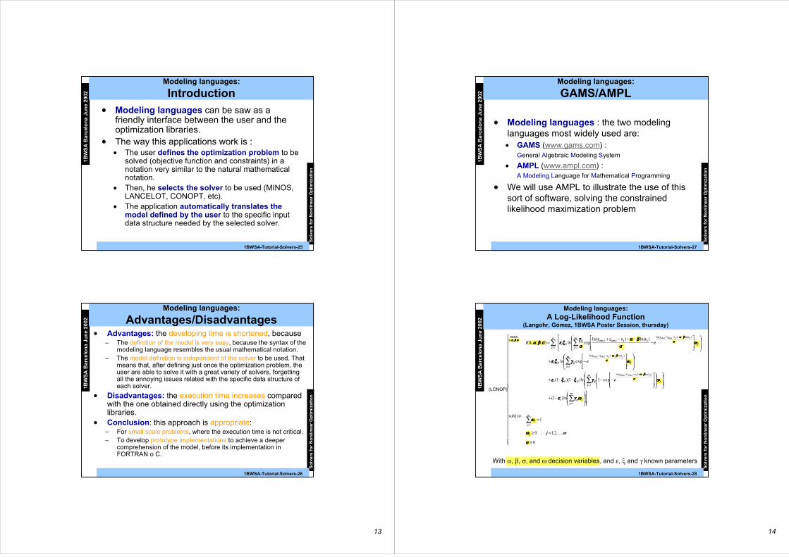
13
1BW
SA
Bar
celo
na
Jun
e 20
02
So
lver
s fo
r N
on
lin
ear
Op
tim
izat
ion
1BWSA-Tutorial-Solvers-25
Modeling languages:
Introduction• Modeling languages can be saw as a
friendly interface between the user and theoptimization libraries.
• The way this applications work is :• The user defines the optimization problem to be
solved (objective function and constraints) in anotation very similar to the natural mathematicalnotation.
• Then, he selects the solver to be used (MINOS,LANCELOT, CONOPT, etc).
• The application automatically translates themodel defined by the user to the specific inputdata structure needed by the selected solver.
1BW
SA
Bar
celo
na
Jun
e 20
02
So
lver
s fo
r N
on
lin
ear
Op
tim
izat
ion
1BWSA-Tutorial-Solvers-26
Modeling languages:
Advantages/Disadvantages• Advantages: the developing time is shortened, because
– The definition of the model is very easy, because the syntax of themodeling language resembles the usual mathematical notation.
– The model definition is independent of the solver to be used. Thatmeans that, after defining just once the optimization problem, theuser are able to solve it with a great variety of solvers, forgettingall the annoying issues related with the specific data structure ofeach solver.
• Disadvantages: the execution time increases comparedwith the one obtained directly using the optimizationlibraries.
• Conclusion: this approach is appropriate:– For small scale problems, where the execution time is not critical.– To develop prototype implementations to achieve a deeper
comprehension of the model, before its implementation inFORTRAN o C.
14
1BW
SA
Bar
celo
na
Jun
e 20
02
So
lver
s fo
r N
on
lin
ear
Op
tim
izat
ion
1BWSA-Tutorial-Solvers-27
Modeling languages:
GAMS/AMPL
• Modeling languages : the two modelinglanguages most widely used are:• GAMS (www.gams.com) :
General Algebraic Modeling System
• AMPL (www.ampl.com) :A Modeling Language for Mathematical Programming
• We will use AMPL to illustrate the use of thissort of software, solving the constrainedlikelihood maximization problem
1BW
SA
Bar
celo
na
Jun
e 20
02
So
lver
s fo
r N
on
lin
ear
Op
tim
izat
ion
1BWSA-Tutorial-Solvers-28
With α, β, σ, and ω decision variables, and ε, ξ and γ known parameters
Modeling languages:A Log-Likelihood Function
(Langohr, Gómez, 1BWSA Poster Session, thursday)
≥
=≥
=
−+
−−−−+
−+
−
−−−+=
∑
∑
∑
∑
∑∑
=
=
=
−−−+
=
−−−+
=
−−−+
=
0
,,2,1,0
1: tosubj.
ln)1(
exp1ln)1)(1(
expln
)ln()ln(expln),,,(
max
m
1j
1
1
)ln()ln(
21
1
)ln()ln(
2
1
)ln()ln(,,
11
,,,
,,
,,
,,
σσσσ
ωωωω
ωωωω
ωωωωγγγγεεεε
ωωωωγγγγξξξξξξξξεεεε
ωωωωγγγγξξξξεεεε
ωωωωσσσσ
ββββαααασσσσγγγγ
ξξξξεεεεσσσσββββαααα
σσσσββββαααα
σσσσββββαααα
σσσσββββαααα
σσσσββββαααα
mj
e
e
esszy
l
j
j
m
jjiji
m
jj
sszy
ijiii
m
jj
sszy
ijii
m
jj
sszyjjiobsiobsij
ii
n
i
jjiobsiobs
jjiobsiobs
jjiobsiobs
K
ùù
(LCNOP)
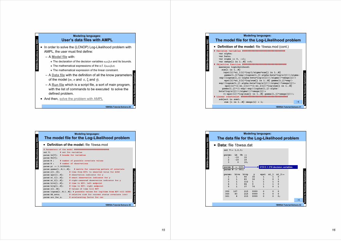
15
1BW
SA
Bar
celo
na
Jun
e 20
02
So
lver
s fo
r N
on
lin
ear
Op
tim
izat
ion
1BWSA-Tutorial-Solvers-29
Modeling languages:
User’s data files with AMPL
• In order to solve the (LCNOP) Log-Likelihood problem withAMPL, the user must first define:
– A Model file with: The declaration of the decision variables ω,α,β,σ and its bounds.
The mathematical expressions of the o.f. l(ω,α,β,σ)
The mathematical expression of the linear constraint.
– A Data file with the definition of all the know parametersof the model (m, n and ε, ξ and γ).
– A Run file which is a script file, a sort of main program,with the list of commands to be executed to solve thedefined problem.
• And then, solve the problem with AMPL
1BW
SA
Bar
celo
na
Jun
e 20
02
So
lver
s fo
r N
on
lin
ear
Op
tim
izat
ion
1BWSA-Tutorial-Solvers-30
Modeling languages:
The model file for the Log-Likelihood problem
# Parameters of the model ##############################
set V; # set for variables
param LbV; # bounds for variables
param UbV;
param M ; # number of possible covariate values
param N ; # number of observations
param pi := 3.14159265;
param gamma1..N,1..M; # matrix for censoring pattern of covariate
param y1..N; # time from HIV+ to observed value for AIDS
param epsi1..N; # observation indicator for y
param xi_11..N; # exact observation indicator for y
param xi_21..N; # right-censored observation indicator for y
param hivn1..N; # time to HIV: left endpoint
param hivp1..N; # time to HIV: right endpoint
param s1..M; # values of time till HIV
param logsum1..N,1..M; # possible values for log(time from HIV till AIDS)
param RR_zeta; # relative risk for current status covariate (csc)
param acc_fac_z; # accelerating factor for csc
• Definition of the model: file 1bwsa.mod
16
1BW
SA
Bar
celo
na
Jun
e 20
02
So
lver
s fo
r N
on
lin
ear
Op
tim
izat
ion
1BWSA-Tutorial-Solvers-31
Modeling languages:
The model file for the Log-Likelihood problem
# Decision variables ################################var alpha;var beta;var sigma >= 0, :=1;var omegaj in 1..M >=0;
# Objective function #################################maximize logLikelihood: sumi in 1..N (epsi[i]*xi_1[i]*log(1/sigma*sumj in 1..M gamma[i,j]*exp((logsum[i,j]-alpha-beta*log(s[j]))/sigma-exp((logsum[i,j]-alpha-beta*log(s[j]))/sigma))*omega[j])+ epsi[i]*xi_2[i]*log(sumj in 1..M gamma[i,j]*exp(-exp((logsum[i,j]-alpha-beta*log(s[j]))/sigma))*omega[j])+
epsi[i]*(1-xi_1[i])*(1-xi_2[i])*log(sumj in 1..M gamma[i,j]*(1-exp(-exp((logsum[i,j]-alpha-
beta*log(s[j]))/sigma)))*omega[j])+ (1-epsi[i])*log(sumj in 1..M gamma[i,j]*omega[j]));
# Linear constraint ###################################subject to sum1: sum i in 1..M omega[i] = 1;
• Definition of the model: file 1bwsa.mod (cont.)
1BW
SA
Bar
celo
na
Jun
e 20
02
So
lver
s fo
r N
on
lin
ear
Op
tim
izat
ion
1BWSA-Tutorial-Solvers-32
Modeling languages:
The data file for the Log-Likelihood problem
set V:= 1,2,3;
param: Lb Ub := 1 -15 15 2 -15 15 3 0 15;
param M := 215;param N := 361;
param: hivn hivp y epsi xi_1 xi_2:= 1 1 45 36 1 1 0 2 1 83 36 1 0 1 3 1 112 1 1 1 0 4 1 84 9 1 1 0 5 1 37 76 1 0 1 ...................................... 359 107 215 9999 0 0 0 360 83 215 9999 0 0 0 361 8 215 9999 0 0 0;
• Data: file 1bwsa.dat
215+3 = 218 decision variables
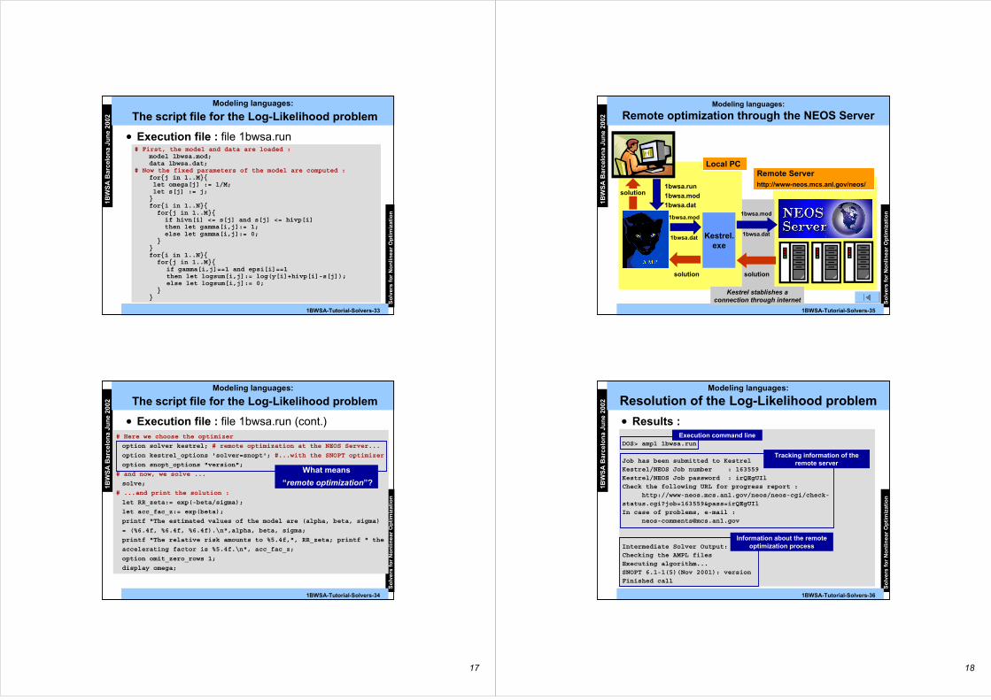
17
1BW
SA
Bar
celo
na
Jun
e 20
02
So
lver
s fo
r N
on
lin
ear
Op
tim
izat
ion
1BWSA-Tutorial-Solvers-33
Modeling languages:
The script file for the Log-Likelihood problem
# First, the model and data are loaded :model 1bwsa.mod;data 1bwsa.dat;
# Now the fixed parameters of the model are computed :forj in 1..M let omega[j] := 1/M; let s[j] := j;fori in 1..N forj in 1..M if hivn[i] <= s[j] and s[j] <= hivp[i] then let gamma[i,j]:= 1; else let gamma[i,j]:= 0; fori in 1..N forj in 1..M if gamma[i,j]==1 and epsi[i]==1 then let logsum[i,j]:= log(y[i]+hivp[i]-s[j]); else let logsum[i,j]:= 0;
• Execution file : file 1bwsa.run
1BW
SA
Bar
celo
na
Jun
e 20
02
So
lver
s fo
r N
on
lin
ear
Op
tim
izat
ion
1BWSA-Tutorial-Solvers-34
# Here we choose the optimizer
option solver kestrel; # remote optimization at the NEOS Server...
option kestrel_options 'solver=snopt'; #...with the SNOPT optimizer
option snopt_options "version";
# and now, we solve ...
solve;
# ...and print the solution :
let RR_zeta:= exp(-beta/sigma);
let acc_fac_z:= exp(beta);
printf "The estimated values of the model are (alpha, beta, sigma)
= (%6.4f, %6.4f, %6.4f).\n",alpha, beta, sigma;
printf "The relative risk amounts to %5.4f,", RR_zeta; printf " the
accelerating factor is %5.4f.\n", acc_fac_z;
option omit_zero_rows 1;
display omega;
Modeling languages:
The script file for the Log-Likelihood problem
• Execution file : file 1bwsa.run (cont.)
What means
“remote optimization”?
18
1BW
SA
Bar
celo
na
Jun
e 20
02
So
lver
s fo
r N
on
lin
ear
Op
tim
izat
ion
1BWSA-Tutorial-Solvers-35
Local PCRemote Serverhttp://www-neos.mcs.anl.gov/neos/
Kestrel stablishes aconnection through internet
Modeling languages:
Remote optimization through the NEOS Server
solution
Kestrel.exe
1bwsa.mod
1bwsa.dat
1bwsa.mod
1bwsa.dat
solution
solution1bwsa.run
1bwsa.mod
1bwsa.dat
1BW
SA
Bar
celo
na
Jun
e 20
02
So
lver
s fo
r N
on
lin
ear
Op
tim
izat
ion
1BWSA-Tutorial-Solvers-36
DOS> ampl 1bwsa.run
Job has been submitted to KestrelKestrel/NEOS Job number : 163559Kestrel/NEOS Job password : irQEgUIlCheck the following URL for progress report : http://www-neos.mcs.anl.gov/neos/neos-cgi/check-status.cgi?job=163559&pass=irQEgUIlIn case of problems, e-mail : [email protected]
Intermediate Solver Output:Checking the AMPL filesExecuting algorithm...SNOPT 6.1-1(5)(Nov 2001): versionFinished call
Modeling languages:
Resolution of the Log-Likelihood problem
• Results :
Tracking information of theremote server
Information about the remoteoptimization process
Execution command line

19
1BW
SA
Bar
celo
na
Jun
e 20
02
So
lver
s fo
r N
on
lin
ear
Op
tim
izat
ion
1BWSA-Tutorial-Solvers-37
Modeling languages:
Resolution of the Log-Likelihood problem
SNOPT 6.1-1(5)(Nov 2001):Optimal solution found.1882 iterations, objective -444.6446856Nonlin evals: obj = 201, grad = 200.
The estimated values of the model are (alpha, beta, sigma) =(4.8218, 0.1374, 0.4752).The relative risk amounts to 0.7490, the accelerating factoris 1.1472.omega [*] := 1 0.0407 6 0.156988 10 0.0827764 24 0.167377 36 0.0762982 48 0.126317 59 0.0737118 60 0.0258302 83 0.0796388 95 0.0172243119 0.073086202 0.0800525
• Results : (cont.) Information sent by the remoteoptimization server
Solution printed by thelocal 1bwsa.run file
Only the nonzero variables ωωωωj are shown