HERMITE AND BERNSTEIN STYLE BASIS FUNCTIONS FOR CUBIC SERENDIPITY

HERMITE AND BERNSTEIN STYLE BASIS FUNCTIONS FOR CUBICSERENDIPITY SPACES ON SQUARES AND CUBES

ANDREW GILLETTE

ABSTRACT. We introduce new Hermite-style and Bernstein-style geometric decompo-sitions of the cubic order serendipity finite element spaces S3(I2) and S3(I3), as definedin the recent work of Arnold and Awanou [Found. Comput. Math. 11 (2011), 337–344].The serendipity spaces are substantially smaller in dimension than the more commonlyused bicubic and tricubic Hermite tensor product spaces - 12 instead of 20 for the squareand 32 instead of 64 for the cube - yet are still guaranteed to obtain cubic order a pri-ori error estimates when used in finite element methods. The basis functions we definehave a canonical relationship both to the finite element degrees of freedom as well asto the geometry of their graphs; this makes the bases ideal for applications employingisogeometric analysis where domain geometry and functions supported on the domainare described by the same basis functions. Moreover, the basis functions are linear com-binations of the commonly used bicubic and tricubic polynomial Bernstein or Hermitebasis functions, allowing their rapid incorporation into existing finite element codes.

1. INTRODUCTION

Serendipity spaces offer a rigorous means to reduce the degrees of freedom associatedto a finite element method while still ensuring optimal order convergence. The ‘serendip-ity’ moniker came from the observation of this phenomenon among finite element prac-titioners before its mathematical justification was fully understood; see e.g. [14, 10, 11,7]. Recent work by Arnold and Awanou [1, 2] classifies serendipity spaces on cubicalmeshes in n ≥ 2 dimensions by giving a simple and precise definition of the space ofpolynomials that must be spanned, as well as a unisolvent set of degrees of freedom forthem. For degree r convergence, the serendipity space is defined as the span of m mono-mials in n variables and is denoted Sr(In).1 Since these m monomials bear no obviouscorrespondence to the m domain points of the n-dimensional unit cube In nor to the mdegrees of freedom described in the papers, alternative local bases for the serendipityspaces must be derived.

In this paper, we provide two coordinate-independent geometric decompositions forboth S3(I2) and S3(I3), the cubic serendipity spaces in two and three dimensions, re-spectively. We present sets of polynomial basis functions associated in a natural andsymmetric fashion to the cubic serendipity domain points of the square or cube andprove that they provide a basis for the corresponding cubic serendipity space. Each basisis designated as either Bernstein or Hermite style, as each function restricts to one ofthese common basis function types on each edge of the square or cube.

The Hermite style bases have the desirable property of being Lagrange-like with re-spect to vertex values and coordinate directional derivative values at vertices. More pre-cisely, if a Hermite style function is associated to a vertex, it has value 1 at that vertex,

Date: August 29, 2012.Key words and phrases. Serendipity spaces, Hermite and Bernstein functions, isogeometric analysis.Supported in part by NSF Award 0715146 and the National Biomedical Computation Resource.1The definition of Sr(In) and its dimension m is reviewed in Section 2.1.

1

2 A. GILLETTE

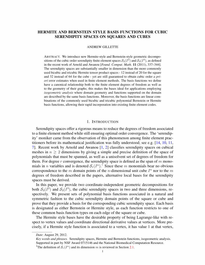
value 0 at other vertices, and coordinate directional derivatives equal to 0 at all vertices.If a Hermite style function is associated to an edge domain point, it has directional deriv-ative equal to 1 at the nearest vertex (in the direction of that domain point) with all othercoordinate directional derivative values equal to 0 (at vertices) and all vertex functionvalues equal to zero. The Bernstein style basis functions have the more simply-statedproperty of obtaining a unique maximal value at the associated domain point. Graphs ofboth types of functions over I2 are shown in Figures 4 and 5.

14(x− 1)(y − 1) −1

4

√32

(x2 − 1) (y − 1) −14

√52x (x2 − 1) (y − 1)

FIGURE 1. Cubic serendipity functions on I2 from [15]. The left functionis associated to the vertex below the peak. The middle and right functionsare associated to the edge y = −1 but do not correspond to the domainpoints (±1

3,−1) in any canonical or symmetric fashion, making them less

useful for geometric modeling or isogeometric analysis.

To the author’s knowledge, the only basis functions previously available for cubic or-der serendipity finite element purposes employ Legendre polynomials, which lack a clearrelationship to the domain points. Definitions of these basis functions can be found inSzabo and Babuska [15, Sections 6.1 and 13.3]; the two functions from [15] associated tothe edge y = −1 of I2, are shown in Figure 1 (middle and right). The restriction of thesefunctions to the edge gives an even polynomial in one case and an odd polynomial in theother, forcing an ad hoc choice of how to associate the functions to the corresponding do-main points (±1

3,−1). On the other hand, as was just described, the functions presented

in this paper do have a natural correspondence to the domain points of the geometry.Maintaining a concrete and canonical relationship between domain points and basis

functions is an essential component of the growing field of isogeometric analysis (IGA).One of the main goals of IGA is to employ basis functions that can be used both forgeometry modeling and finite element analysis, exactly as we provide here for cubicserendipity spaces. Each function is a linear combination of bicubic or tricubic Bern-stein or Hermite polynomials; the specific coefficients of the combination are given inthe proofs of the theorems. This makes the incorporation of the functions into a vari-ety of existing application contexts relatively easy. Note that tensor product bases intwo and three dimensions are commonly available in finite element software packages(e.g. deal.II [4]) and cubic order tensor products in particular are commonly used both inmodern theory (e.g. isogeometric analysis [9]) and applications (e.g. cardiac electrophys-iology models [16]). Hence, a variety of areas of computational science could directlyemploy the new cubic order serendipity basis functions presented here.

The benefit of serendipity finite element methods is a significant reduction in the com-putational effort required for optimal order (in this case, cubic) convergence. Cubic

HERMITE AND BERNSTEIN STYLE BASIS FUNCTIONS FOR CUBIC SERENDIPITY SPACES 3

serendipity methods on meshes of squares requires 12 functions per element, an im-provement over the 16 functions per element required for bicubic tensor product meth-ods. On meshes of cubes, the cubic serendipity method requires 32 functions per elementinstead of the 64 functions per element required for tricubic tensor product methods. Us-ing fewer basis functions per element reduces the size of the overall linear system thatmust be solved, thereby saving computational time and effort. An additional computa-tional advantage occurs when the functions presented here are used in an isogeometricfashion. The process of converting between computational geometry bases and finiteelement bases is a well-known computational bottleneck in engineering applications [8]but is easily avoided when basis functions suited to both purposes are employed.

The outline of the paper is as follows. In Section 2, we fix notation and summarizerelevant background on Hermite and barycentric basis functions as well as serendipityspaces. In Section 3, we present polynomial Bernstein and Hermite style basis functionsfor S3(I2) that agree with the standard bicubics on edges of I2 and provide a novel geo-metric decomposition of the space. In Section 4, we present polynomial Bernstein andHermite style basis functions for S3(I3) that agree with the standard tricubics on edgesof I3, reduce to our bases for I2 on faces of I3, and provide a novel geometric decom-position of the space. Finally, we state our conclusions and discuss future directions inSection 5.

2. BACKGROUND AND NOTATION

2.1. Serendipity Elements. We first review the definition of serendipity spaces andtheir accompanying notation from the work of Arnold and Awanou [1, 2].

Definition 2.1. The superlinear degree of a monomial in n variables, denoted sldeg(·),is given by

sldeg(xe11 xe22 · · ·xenn ) :=

(n∑

i=1

ei

)− |{ei : ei = 1}| (2.1)

In words, sldeg(q) is the ordinary degree of q, ignoring variables that enter linearly.For instance, the superlinear degree of xy2z3 is 5.

Definition 2.2. Define the following spaces of polynomials, each of which is restrictedto the domain In = [−1, 1]n ⊂ Rn:

Pr(In) := spanR {monomials in n variables with degree ≤ r}

Sr(In) := spanR {monomials in n variables with superlinear degree ≤ r}Qr(I

n) := spanR {monomials in n variables with each variable degree ≤ r}Note that Pr(I

n) ⊂ Sr(In) ⊂ Qr(In), with proper containments when r, n > 1. The

space Sr(In) is called the degree r serendipity space on the n-dimensional unit cube In.In the notation of the more recent paper by Arnold and Awanou [2], the serendipity spacesdiscussed in this work would be denoted SrΛ0(In), indicating that they are differential0-form spaces. The spaces have dimension given by the following formulas (cf. [1]).

dimPr(In) =

(n+ r

n

)dimSr(In) =

min(n,br/2c)∑d=0

2n−d(n

d

)(r − dd

)dimQr(I

n) = (r + 1)n

4 A. GILLETTE

We write out standard bases for these spaces more precisely in the cubic order cases ofconcern here.

P3(I2) = span{ 1 , x, y︸︷︷︸

linear

, x2, y2, xy︸︷︷︸quadratic

, x3, y3, x2y, xy2︸︷︷︸cubic

} (2.2)

S3(I2) = P3(I2) ∪ span{ x3y, xy3︸︷︷︸

superlinear cubic

} (2.3)

Q3(I2) = S3(I2) ∪ span{x2y2, x3y2, x2y3, x3y3} (2.4)

Observe that the dimensions of the three spaces are 10, 12, and 16, respectively.

P3(I3) = span{1, x, y, z︸︷︷︸

linear

, x2, y2, z2, xy, xz, yz︸︷︷︸quadratic

, x3, y3, z3, x2y, x2z, xy2, y2z, xz2, yz2, xyz︸︷︷︸cubic

}

(2.5)

S3(I3) = P3(I3) ∪ span{x3y, x3z, y3z, xy3, xz3, yz3, x2yz, xy2z, xyz2, x3yz, xy3z, xyz3︸︷︷︸

superlinear cubic

}

(2.6)

Q3(I3) = S3(I3) ∪ span{x3y2, . . . , x3y3z3} (2.7)

Observe that the dimensions of the three spaces are 20, 32, and 64, respectively.The serendipity spaces are associated to specific degrees of freedom in the classical

finite element sense. For a face f of In of dimension d ≥ 0, the degrees of freedomassociated to f for Sr(In) are (cf. [1])

u 7−→∫f

uq, q ∈ Pr−2d(f).

For the cases considered in this work, n = 2 or 3 and r = 3 so the only non-zero degreesof freedom are when f is a vertex (d = 0) or an edge (d = 1). Thus, the degrees offreedom for our cases are the values

u(v),

∫e

u dt, and∫e

ut dt, (2.8)

for each vertex v and each edge e of the square or cube.

0.0 0.2 0.4 0.6 0.8 1.0

0.2

0.4

0.6

0.8

1.0

0.0 0.2 0.4 0.6 0.8 1.0

0.2

0.4

0.6

0.8

1.0

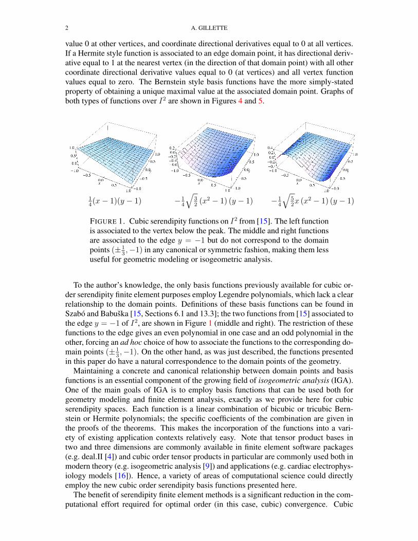
FIGURE 2. The Bernstein basis [β] and the Hermite basis [ψ] on [0, 1].

2.2. Cubic Bernstein and Hermite Bases. For cubic order approximation on square orcubical grids, tensor product bases are typically built from one of two alternative bases


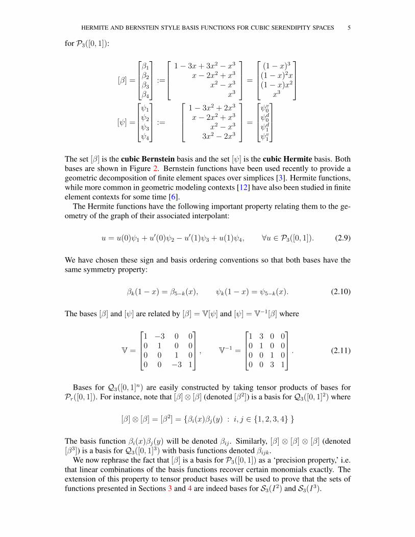
for P3([0, 1]):

[β] =

β1β2β3β4

:=

1− 3x+ 3x2 − x3

x− 2x2 + x3

x2 − x3x3

=

(1− x)3

(1− x)2x(1− x)x2

x3

[ψ] =

ψ1

ψ2

ψ3

ψ4

:=

1− 3x2 + 2x3

x− 2x2 + x3

x2 − x33x2 − 2x3

=

ψv0

ψd0

ψd1

ψv1

The set [β] is the cubic Bernstein basis and the set [ψ] is the cubic Hermite basis. Bothbases are shown in Figure 2. Bernstein functions have been used recently to provide ageometric decomposition of finite element spaces over simplices [3]. Hermite functions,while more common in geometric modeling contexts [12] have also been studied in finiteelement contexts for some time [6].

The Hermite functions have the following important property relating them to the ge-ometry of the graph of their associated interpolant:

u = u(0)ψ1 + u′(0)ψ2 − u′(1)ψ3 + u(1)ψ4, ∀u ∈ P3([0, 1]). (2.9)

We have chosen these sign and basis ordering conventions so that both bases have thesame symmetry property:

βk(1− x) = β5−k(x), ψk(1− x) = ψ5−k(x). (2.10)

The bases [β] and [ψ] are related by [β] = V[ψ] and [ψ] = V−1[β] where

V =

1 −3 0 00 1 0 00 0 1 00 0 −3 1

, V−1 =

1 3 0 00 1 0 00 0 1 00 0 3 1

. (2.11)

Bases for Q3([0, 1]n) are easily constructed by taking tensor products of bases forPr([0, 1]). For instance, note that [β]⊗ [β] (denoted [β2]) is a basis forQ3([0, 1]2) where

[β]⊗ [β] = [β2] = {βi(x)βj(y) : i, j ∈ {1, 2, 3, 4} }

The basis function βi(x)βj(y) will be denoted βij . Similarly, [β] ⊗ [β] ⊗ [β] (denoted[β3]) is a basis for Q3([0, 1]3) with basis functions denoted βijk.

We now rephrase the fact that [β] is a basis for P3([0, 1]) as a ‘precision property,’ i.e.that linear combinations of the basis functions recover certain monomials exactly. Theextension of this property to tensor product bases will be used to prove that the sets offunctions presented in Sections 3 and 4 are indeed bases for S3(I2) and S3(I3).

6 A. GILLETTE

Proposition 2.3. For 0 ≤ r, s, t ≤ 3, the precision properties of [β], [β2], and [β3] takeon the respective forms

xr =4∑

i=1

(3− r4− i

)βi, (2.12)

xrys =4∑

i=1

4∑j=1

(3− r4− i

)(3− s4− j

)βij, (2.13)

xryszt =4∑

i=1

4∑j=1

4∑k=1

(3− r4− i

)(3− s4− j

)(3− t4− k

)βijk. (2.14)

Proof. One easily confirms that x3 = β4, x2 = β4 + β3, x1 = β4 + 2β3 + β2, andx0 = β4 + 3β3 + 3β2 + β1, which is the statement of (2.12). The other two statementsfollow immediately from the first. �

We have a similar proposition for the Hermite basis [ψ] and its tensor products [ψ2] :=[ψ]⊗ [ψ] and [ψ3] := [ψ]⊗ [ψ]⊗ [ψ]. As before, ψij means ψi(x)ψj(y) and ψijk meansψi(x)ψj(y)ψk(z).

Proposition 2.4. Let

εr,i :=4∑

a=1

(3− r4− a

)vai (2.15)

where vai denotes the (a, i) entry (row, column) of V from (2.11). For 0 ≤ r, s, t ≤ 3, theprecision properties of [ψ], [ψ2], and [ψ3] take on the respective forms

xr =4∑

i=1

εr,iψi, (2.16)

xrys =4∑

i=1

4∑j=1

εr,iεs,jψij, (2.17)

xryszt =4∑

i=1

4∑j=1

4∑k=1

εr,iεs,jεt,kψijk. (2.18)

Proof. By swapping the order of summation, we see that4∑

i=1

εr,iψi =4∑

a=1

(3− r4− a

)( 4∑i=1

vaiψi

)=

4∑a=1

(3− r4− a

)βa = xr,

by (2.12), proving (2.16). The other two statements follow immediately from the first.�

Transforming the bases [β] and [ψ] to domains other than [0, 1] is straightforward. IfT : [a, b]→ [0, 1] is linear, then replacing x with T (x) in each basis function expressionfor [β] and [ψ] gives bases for P3([a, b]). Note, however, that the derivative interpolationproperty for [ψ] must be adjusted to account for the scaling:

u = u(1)ψ1(T (x)) + |b− a|u′(0)ψ2(T (x))

− |b− a|u′(1)ψ3(T (x)) + u(1)ψ4(T (x)), ∀u ∈ P3([a, b]).(2.19)


In geometric modeling applications, the coefficient |b − a| is sometimes left as an ad-justable parameter, usually denoted s for scale factor. [5, 16]. For all the Hermite andHermite style functions, we will use derivative-preserving scaling which will includescale factors on those functions related to derivatives; this will be made explicit in thevarious contexts where it is relevant.

Remark 2.5. Both [β] and [ψ] are Lagrange like at the endpoints of [0, 1], i.e. at anendpoint, the only basis function with non-zero value is the function associated to thatendpoint (β1 or ψ1 for 0, β4 or ψ4 for 1). This means the two remaining basis functions ofeach type (β2, β3 or ψ2, ψ3) are naturally associated to the two edge degrees of freedom(2.8). We will refer to these associations between basis functions and geometrical objectsas the standard geometrical decompositions of [β] and [ψ].

3. LOCAL BASES FOR S3(I2)

11 21 31 41

2212 32 42

2313 33 43

2414 34 44

11 21 31 41

12 42

13 43

2414 34 44

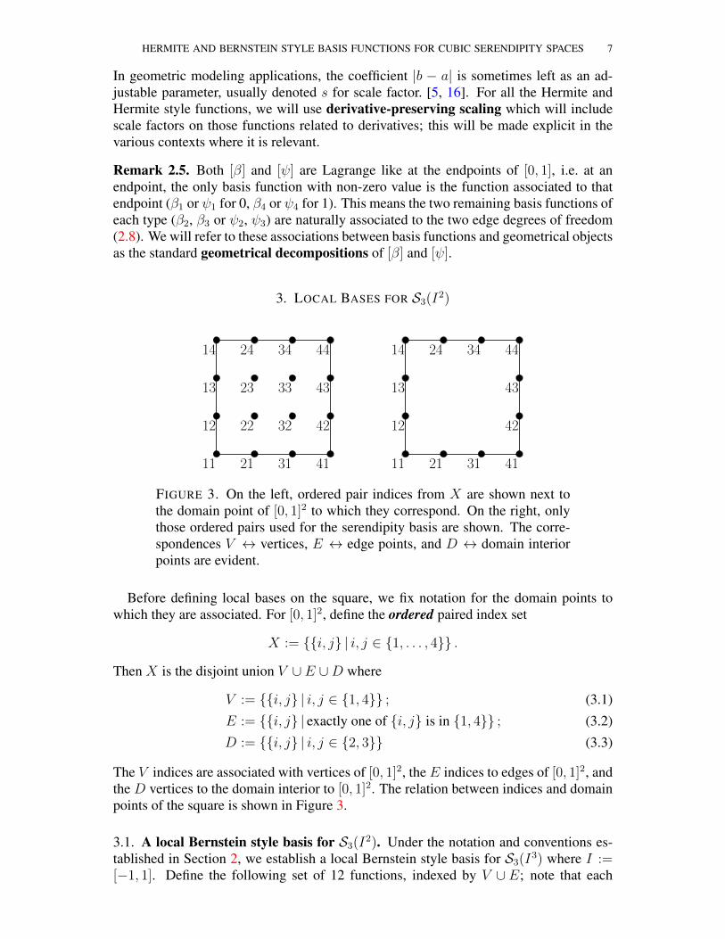
FIGURE 3. On the left, ordered pair indices from X are shown next tothe domain point of [0, 1]2 to which they correspond. On the right, onlythose ordered pairs used for the serendipity basis are shown. The corre-spondences V ↔ vertices, E ↔ edge points, and D ↔ domain interiorpoints are evident.

Before defining local bases on the square, we fix notation for the domain points towhich they are associated. For [0, 1]2, define the ordered paired index set

X := {{i, j} | i, j ∈ {1, . . . , 4}} .

Then X is the disjoint union V ∪ E ∪D where

V := {{i, j} | i, j ∈ {1, 4}} ; (3.1)

E := {{i, j} | exactly one of {i, j} is in {1, 4}} ; (3.2)

D := {{i, j} | i, j ∈ {2, 3}} (3.3)

The V indices are associated with vertices of [0, 1]2, the E indices to edges of [0, 1]2, andthe D vertices to the domain interior to [0, 1]2. The relation between indices and domainpoints of the square is shown in Figure 3.

3.1. A local Bernstein style basis for S3(I2). Under the notation and conventions es-tablished in Section 2, we establish a local Bernstein style basis for S3(I3) where I :=[−1, 1]. Define the following set of 12 functions, indexed by V ∪ E; note that each

8 A. GILLETTE

function is to be scaled by a factor of 1/16.

[ξ2] =

ξ11ξ14ξ41ξ44ξ12ξ13ξ42ξ43ξ21ξ31ξ24ξ34

=

(x− 1)(y − 1)(−2− 2x+ x2 − 2y + y2)−(x− 1)(y + 1)(−2− 2x+ x2 + 2y + y2)−(x+ 1)(y − 1)(−2 + 2x+ x2 − 2y + y2)(x+ 1)(y + 1)(−2 + 2x+ x2 + 2y + y2)

−(x− 1)(y − 1)2(y + 1)(x− 1)(y − 1)(y + 1)2

(x+ 1)(y − 1)2(y + 1)−(x+ 1)(y − 1)(y + 1)2

−(x− 1)2(x+ 1)(y − 1)(x− 1)(x+ 1)2(y − 1)(x− 1)2(x+ 1)(y + 1)−(x− 1)(x+ 1)2(y + 1)

· 1

16(3.4)

Fix the basis orderings

[ξ2] := [ ξ11, ξ14, ξ41, ξ44︸︷︷︸indices in V

, ξ12, ξ13, ξ42, ξ43, ξ21, ξ31, ξ24, ξ34︸︷︷︸indices in E

], (3.5)

[β2] := [ β11, β14, β41, β44︸︷︷︸indices in V

, β12, β13, β42, β43, β21, β31, β24, β34︸︷︷︸indices in E

, β22, β23, β32, β33︸︷︷︸indices in D

] (3.6)

βI11 βI

21 βI31

ξ11 ξ21 ξ31

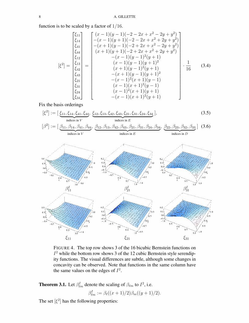
FIGURE 4. The top row shows 3 of the 16 bicubic Bernstein functions onI2 while the bottom row shows 3 of the 12 cubic Bernstein style serendip-ity functions. The visual differences are subtle, although some changes inconcavity can be observed. Note that functions in the same column havethe same values on the edges of I2.

Theorem 3.1. Let βI`m denote the scaling of β`m to I2, i.e.

βI`m := β`((x+ 1)/2)βm((y + 1)/2).

The set [ξ2] has the following properties:


(i) [ξ2] is a basis for S3(I2).(ii) For any `m ∈ V ∪ E, ξ`m is identical to βI

`m on the edges of I2.(iii) [ξ2] is a geometric decomposition of S3(I2).

Proof. For (i), we scale [ξ2] to [0, 1]2 to take advantage of a simple characterization of theprecision properties. Let [ξ2][0,1] denote the set of scaled basis functions ξ[0,1]`m (x, y) :=ξ`m(2x− 1, 2y− 1). Given the basis orderings in (3.5)-(3.6), it can be confirmed directlythat [ξ2][0,1] is related to [β2] by

[ξ2][0,1] = B[β2] (3.7)

where B is the 12× 16 matrix with the structure

B :=[I B′

], (3.8)

where I is the 12× 12 identity matrix and B′ is the 12× 4 matrix

B′ =

−4 −2 −2 −1−2 −4 −1 −2−2 −1 −4 −2−1 −2 −2 −42 0 1 00 2 0 11 0 2 00 1 0 22 1 0 00 0 2 11 2 0 00 0 1 2

. (3.9)

Using ij ∈ X to denote an index for βij and `m ∈ V ∪ E to denote an index for ξ[0,1]`m ,the entries of B can be denoted by b`mij so that

B :=

b1111 · · · b11ij · · · b1133... . . . ... . . . ...b`m11 · · · b`mij · · · b`m33

... . . . ... . . . ...b3411 · · · b34ij · · · b3433

. (3.10)

We now observe that for each ij ∈ X ,(3− r4− i

)(3− s4− j

)=

∑`m∈V ∪E

(3− r4− `

)(3− s4−m

)b`mij , (3.11)

for all (r, s) pairs such that sldeg(xrys) ≤ 3 (recall Definition 2.1). Note that this claimholds trivially for the first 12 columns of B, i.e. for those ij ∈ V ∪ E ⊂ X . Forij ∈ D ⊂ X , (3.11) defines an invertible linear system of 12 equations with 12 unknownswhose solution is the ij column of B′; the 12 (r, s) pairs correspond to the exponents of xand y in the basis ordering of S3(I2) given in (2.2)-(2.3). Substituting (3.11) into (2.13)yields:

xrys =∑ij∈X

( ∑`m∈V ∪E

(3− r4− `

)(3− s4−m

)b`mij

)βij

10 A. GILLETTE

Swapping the order of summation and regrouping yields

xrys =∑

`m∈V ∪E

(3− r4− `

)(3− s4−m

)(∑ij∈X

b`mij βij

).

The inner summation is exactly ξ[0,1]`m by (3.7), implying that

xrys =∑

`m∈V ∪E

(3− r4− `

)(3− s4−m

)ξ[0,1]`m , (3.12)

for all (r, s) pairs with sldeg(xrys) ≤ 3. Since [ξ2][0,1] has 12 elements which span the12 dimensional space S3([0, 1]2), it is a basis for S3([0, 1]2). By scaling, [ξ2] is a basisfor S3(I2).

For (ii), note that an edge of [0, 1]2 is described by an equation of the form {x or y} ={0 or 1}. Since β2(t) and β3(t) are equal to 0 at t = 0 and t = 1, βij ≡ 0 on the edges of[0, 1]2 for any ij ∈ D. By the structure of B from (3.8), we see that for any `m ∈ V ∪E,

ξ[0,1]`m = β`m +

∑ij∈D

b`mij βij. (3.13)

Thus, on the edges of [0, 1]2, ξ[0,1]`m and β`m are identical. After scaling back, we have ξ`mand βI

`m identical on the edges of I2, as desired.For (iii), the geometric decomposition is given by the indices of the basis functions,

i.e. the function ξ`m is associated to the domain point for `m ∈ V ∪ E. This followsimmediately from (ii), the fact that [β2] is a tensor product basis, and Remark 2.5.

�

Remark 3.2. It is worth noting that the basis [ξ2] was derived by essentially the reverseorder of the proof of part (i) of the theorem. More precisely, the twelve coefficients ineach column of B define an invertible linear system given by (3.11). After solving for thecoefficients, we can immediately derive the basis functions via (3.7). By the nature of thisapproach, the edge agreement property (ii) is guaranteed by the symmetry properties ofthe basis [β]. This technique was inspired by a previous work for Lagrange-like quadraticserendipity elements on convex polygons [13].

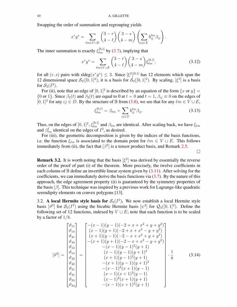
3.2. A local Hermite style basis for S3(I2). We now establish a local Hermite stylebasis [ϑ2] for S3(I2) using the bicubic Hermite basis [ψ2] for Q3([0, 1]2). Define thefollowing set of 12 functions, indexed by V ∪ E; note that each function is to be scaledby a factor of 1/8.

[ϑ2] =

ϑ11

ϑ14

ϑ41

ϑ44

ϑ12

ϑ13

ϑ42

ϑ43

ϑ21

ϑ31

ϑ24

ϑ34

=

−(x− 1)(y − 1)(−2 + x+ x2 + y + y2)(x− 1)(y + 1)(−2 + x+ x2 − y + y2)(x+ 1)(y − 1)(−2− x+ x2 + y + y2)−(x+ 1)(y + 1)(−2− x+ x2 − y + y2)

−(x− 1)(y − 1)2(y + 1)(x− 1)(y − 1)(y + 1)2

(x+ 1)(y − 1)2(y + 1)−(x+ 1)(y − 1)(y + 1)2

−(x− 1)2(x+ 1)(y − 1)(x− 1)(x+ 1)2(y − 1)(x− 1)2(x+ 1)(y + 1)−(x− 1)(x+ 1)2(y + 1)

· 1

8(3.14)


Fix the basis orderings

[ϑ2] := [ ϑ11, ϑ14, ϑ41, ϑ44︸︷︷︸indices in V

, ϑ12, ϑ13, ϑ42, ϑ43, ϑ21, ϑ31, ϑ24, ϑ34︸︷︷︸indices in E

], (3.15)

[ψ2] := [ ψ11, ψ14, ψ41, ψ44︸︷︷︸indices in V

, ψ12, ψ13, ψ42, ψ43, ψ21, ψ31, ψ24, ψ34︸︷︷︸indices in E

, ψ22, ψ23, ψ32, ψ33︸︷︷︸indices in D

]

(3.16)

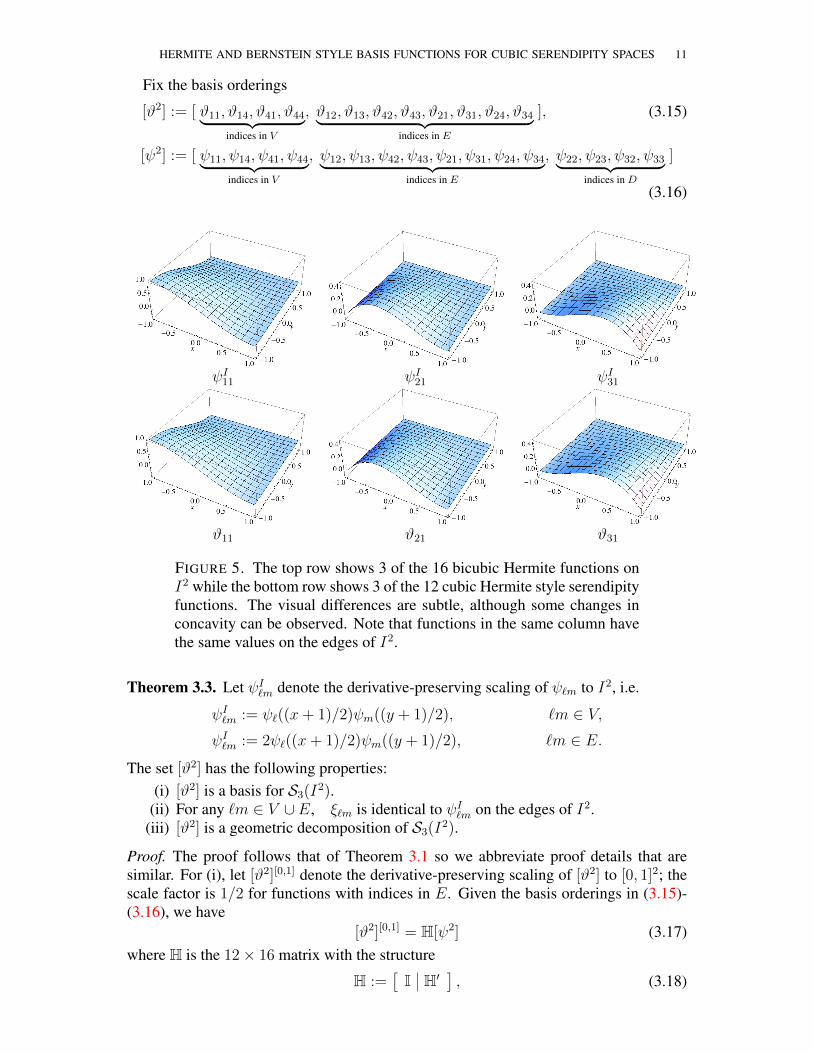
ψI11 ψI

21 ψI31

ϑ11 ϑ21 ϑ31

FIGURE 5. The top row shows 3 of the 16 bicubic Hermite functions onI2 while the bottom row shows 3 of the 12 cubic Hermite style serendipityfunctions. The visual differences are subtle, although some changes inconcavity can be observed. Note that functions in the same column havethe same values on the edges of I2.

Theorem 3.3. Let ψI`m denote the derivative-preserving scaling of ψ`m to I2, i.e.

ψI`m := ψ`((x+ 1)/2)ψm((y + 1)/2), `m ∈ V,ψI`m := 2ψ`((x+ 1)/2)ψm((y + 1)/2), `m ∈ E.

The set [ϑ2] has the following properties:(i) [ϑ2] is a basis for S3(I2).

(ii) For any `m ∈ V ∪ E, ξ`m is identical to ψI`m on the edges of I2.

(iii) [ϑ2] is a geometric decomposition of S3(I2).

Proof. The proof follows that of Theorem 3.1 so we abbreviate proof details that aresimilar. For (i), let [ϑ2][0,1] denote the derivative-preserving scaling of [ϑ2] to [0, 1]2; thescale factor is 1/2 for functions with indices in E. Given the basis orderings in (3.15)-(3.16), we have

[ϑ2][0,1] = H[ψ2] (3.17)where H is the 12× 16 matrix with the structure

H :=[I H′

], (3.18)

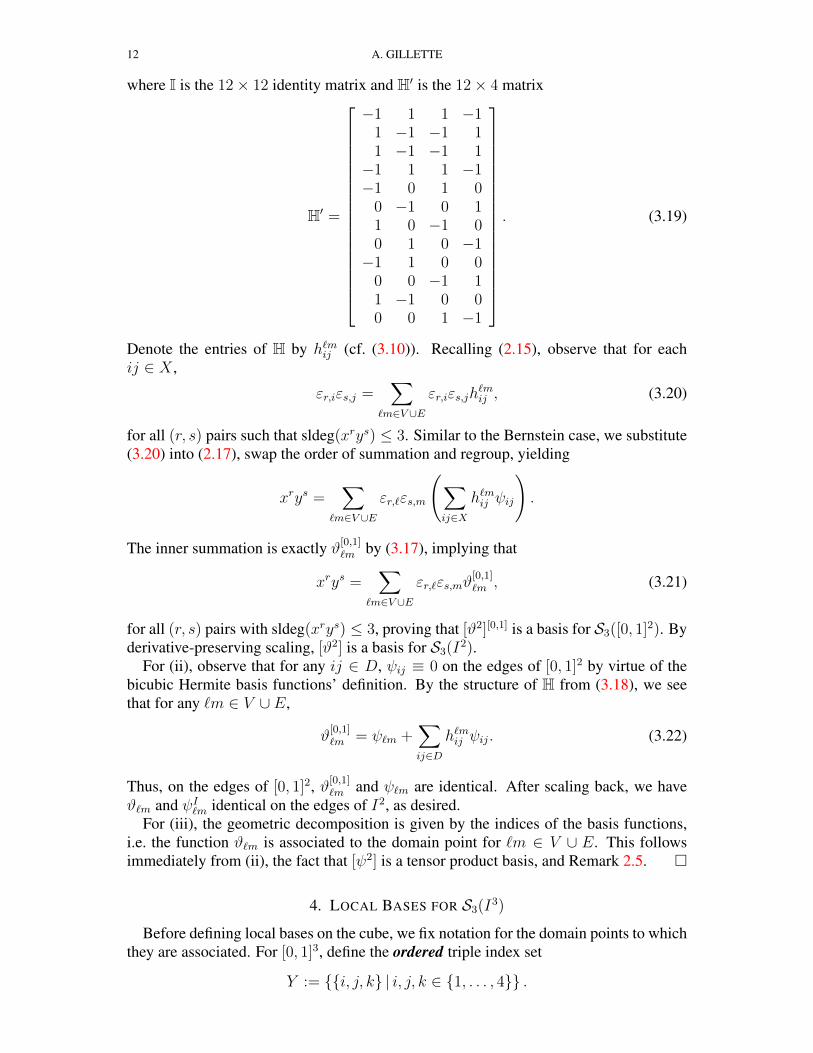
12 A. GILLETTE

where I is the 12× 12 identity matrix and H′ is the 12× 4 matrix

H′ =

−1 1 1 −11 −1 −1 11 −1 −1 1−1 1 1 −1−1 0 1 0

0 −1 0 11 0 −1 00 1 0 −1−1 1 0 0

0 0 −1 11 −1 0 00 0 1 −1

. (3.19)

Denote the entries of H by h`mij (cf. (3.10)). Recalling (2.15), observe that for eachij ∈ X ,

εr,iεs,j =∑

`m∈V ∪E

εr,iεs,jh`mij , (3.20)

for all (r, s) pairs such that sldeg(xrys) ≤ 3. Similar to the Bernstein case, we substitute(3.20) into (2.17), swap the order of summation and regroup, yielding

xrys =∑

`m∈V ∪E

εr,`εs,m

(∑ij∈X

h`mij ψij

).

The inner summation is exactly ϑ[0,1]`m by (3.17), implying that

xrys =∑

`m∈V ∪E

εr,`εs,mϑ[0,1]`m , (3.21)

for all (r, s) pairs with sldeg(xrys) ≤ 3, proving that [ϑ2][0,1] is a basis for S3([0, 1]2). Byderivative-preserving scaling, [ϑ2] is a basis for S3(I2).

For (ii), observe that for any ij ∈ D, ψij ≡ 0 on the edges of [0, 1]2 by virtue of thebicubic Hermite basis functions’ definition. By the structure of H from (3.18), we seethat for any `m ∈ V ∪ E,

ϑ[0,1]`m = ψ`m +

∑ij∈D

h`mij ψij. (3.22)

Thus, on the edges of [0, 1]2, ϑ[0,1]`m and ψ`m are identical. After scaling back, we have

ϑ`m and ψI`m identical on the edges of I2, as desired.

For (iii), the geometric decomposition is given by the indices of the basis functions,i.e. the function ϑ`m is associated to the domain point for `m ∈ V ∪ E. This followsimmediately from (ii), the fact that [ψ2] is a tensor product basis, and Remark 2.5. �

4. LOCAL BASES FOR S3(I3)

Before defining local bases on the cube, we fix notation for the domain points to whichthey are associated. For [0, 1]3, define the ordered triple index set

Y := {{i, j, k} | i, j, k ∈ {1, . . . , 4}} .


111 211

112 212

113 213

114 214

121

122

123

124

131

132

133

134

141

142

143

144

311

312

313

314

411

412

413

414

411

244 344 444

234 334 444

224 324 444

111 211

112

113

114 214

121

124

131

134

141

142

143

144

311

314

411

412

413

414

411

244 344 444

444

444

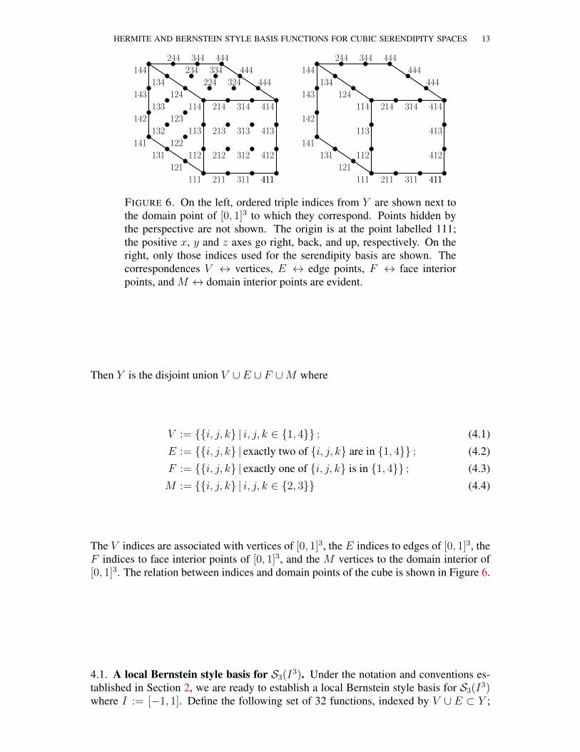
FIGURE 6. On the left, ordered triple indices from Y are shown next tothe domain point of [0, 1]3 to which they correspond. Points hidden bythe perspective are not shown. The origin is at the point labelled 111;the positive x, y and z axes go right, back, and up, respectively. On theright, only those indices used for the serendipity basis are shown. Thecorrespondences V ↔ vertices, E ↔ edge points, F ↔ face interiorpoints, and M ↔ domain interior points are evident.

Then Y is the disjoint union V ∪ E ∪ F ∪M where

V := {{i, j, k} | i, j, k ∈ {1, 4}} ; (4.1)

E := {{i, j, k} | exactly two of {i, j, k} are in {1, 4}} ; (4.2)

F := {{i, j, k} | exactly one of {i, j, k} is in {1, 4}} ; (4.3)

M := {{i, j, k} | i, j, k ∈ {2, 3}} (4.4)

The V indices are associated with vertices of [0, 1]3, the E indices to edges of [0, 1]3, theF indices to face interior points of [0, 1]3, and the M vertices to the domain interior of[0, 1]3. The relation between indices and domain points of the cube is shown in Figure 6.

4.1. A local Bernstein style basis for S3(I3). Under the notation and conventions es-tablished in Section 2, we are ready to establish a local Bernstein style basis for S3(I3)where I := [−1, 1]. Define the following set of 32 functions, indexed by V ∪ E ⊂ Y ;

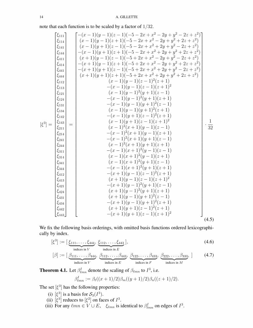
14 A. GILLETTE

note that each function is to be scaled by a factor of 1/32.

[ξ3] =

ξ111ξ114ξ141ξ144ξ411ξ414ξ441ξ444ξ112ξ113ξ121ξ124ξ131ξ134ξ142ξ143ξ211ξ214ξ241ξ244ξ311ξ314ξ341ξ344ξ412ξ413ξ421ξ424ξ431ξ434ξ442ξ443

=

−(x− 1)(y − 1)(z − 1)(−5− 2x+ x2 − 2y + y2 − 2z + z2)(x− 1)(y − 1)(z + 1)(−5− 2x+ x2 − 2y + y2 + 2z + z2)(x− 1)(y + 1)(z − 1)(−5− 2x+ x2 + 2y + y2 − 2z + z2)−(x− 1)(y + 1)(z + 1)(−5− 2x+ x2 + 2y + y2 + 2z + z2)(x+ 1)(y − 1)(z − 1)(−5 + 2x+ x2 − 2y + y2 − 2z + z2)−(x+ 1)(y − 1)(z + 1)(−5 + 2x+ x2 − 2y + y2 + 2z + z2)−(x+ 1)(y + 1)(z − 1)(−5 + 2x+ x2 + 2y + y2 − 2z + z2)(x+ 1)(y + 1)(z + 1)(−5 + 2x+ x2 + 2y + y2 + 2z + z2)

(x− 1)(y − 1)(z − 1)2(z + 1)−(x− 1)(y − 1)(z − 1)(z + 1)2

(x− 1)(y − 1)2(y + 1)(z − 1)−(x− 1)(y − 1)2(y + 1)(z + 1)−(x− 1)(y − 1)(y + 1)2(z − 1)(x− 1)(y − 1)(y + 1)2(z + 1)−(x− 1)(y + 1)(z − 1)2(z + 1)(x− 1)(y + 1)(z − 1)(z + 1)2

(x− 1)2(x+ 1)(y − 1)(z − 1)−(x− 1)2(x+ 1)(y − 1)(z + 1)−(x− 1)2(x+ 1)(y + 1)(z − 1)(x− 1)2(x+ 1)(y + 1)(z + 1)−(x− 1)(x+ 1)2(y − 1)(z − 1)(x− 1)(x+ 1)2(y − 1)(z + 1)(x− 1)(x+ 1)2(y + 1)(z − 1)−(x− 1)(x+ 1)2(y + 1)(z + 1)−(x+ 1)(y − 1)(z − 1)2(z + 1)(x+ 1)(y − 1)(z − 1)(z + 1)2

−(x+ 1)(y − 1)2(y + 1)(z − 1)(x+ 1)(y − 1)2(y + 1)(z + 1)(x+ 1)(y − 1)(y + 1)2(z − 1)−(x+ 1)(y − 1)(y + 1)2(z + 1)(x+ 1)(y + 1)(z − 1)2(z + 1)−(x+ 1)(y + 1)(z − 1)(z + 1)2

· 1

32

(4.5)

We fix the following basis orderings, with omitted basis functions ordered lexicographi-cally by index.

[ξ3] := [ ξ111, . . . , ξ444︸︷︷︸indices in V

, ξ112, . . . , ξ443︸︷︷︸indices in E

], (4.6)

[β] := [ β111, . . . , β444︸︷︷︸indices in V

, β112, . . . , β443︸︷︷︸indices in E

, β122, . . . , β433︸︷︷︸indices in F

, β222, . . . , β333︸︷︷︸indices in M

, ] (4.7)

Theorem 4.1. Let βI`mn denote the scaling of β`mn to I3, i.e.

βI`mn := β`((x+ 1)/2)βm((y + 1)/2)βn((z + 1)/2).

The set [ξ3] has the following properties:(i) [ξ3] is a basis for S3(I3).

(ii) [ξ3] reduces to [ξ2] on faces of I3.(iii) For any `mn ∈ V ∪ E, ξ`mn is identical to βI

`mn on edges of I3.


(iv) [ξ3] is a geometric decomposition of S3(I3).

Proof. The proof is similar to that of Theorem 3.1 so we abbreviate some details. For (i),let [ξ3][0,1] denote the scaling of [ξ3] to [0, 1]3. Given the basis orderings in (4.6)-(4.7),we have

[ξ3][0,1] = U[β3] (4.8)

where U is the 32× 64 matrix with the structure

U :=[I U′

], (4.9)

where I is the 32 × 32 identity matrix and U′ is a specific 32 × 32 matrix whose entriesare integers ranging from -16 to 4. Instead of writing out U′ in its entirety, we describeits properties and how it can be constructed (cf. Remark 3.2).

Using ijk ∈ Y to denote an index for βijk and `mn ∈ V ∪ E ⊂ Y to denote an indexfor ξ[0,1]`mn, the entries of U will be denoted by k`mn

ijk so that

U :=

u111111 · · · u111ijk · · · u111333

... . . . ... . . . ...u`mn111 · · · u`mn

ijk · · · u`mn333

... . . . ... . . . ...u443111 · · · u443ijk · · · u443333

. (4.10)

The columns of U satisfy the relationship(3− r4− i

)(3− s4− j

)(3− t4− k

)=

∑`mn∈V ∪E

(3− r4− `

)(3− s4−m

)(3− t4− n

)u`mnijk , (4.11)

for all (r, s, t) tuples such that sldeg(xryszt) ≤ 3. This property defines the entries of Uuniquely since for each ijk ∈ Y it gives an invertible linear system of 32 equations with32 unknowns whose solution is the ijk column of U. The (r, s, t) tuples should be takenin the order given in (2.5)-(2.6). See Remark 3.2 and the text after (3.11) for more onthis process.

As in previous proofs, regrouping and recognizing an expression for ξ[0,1]`mn gives

xryszt =∑

`mn∈V ∪E

(3− r4− `

)(3− s4−m

)(3− t4− n

)ξ`mn, (4.12)

proving, after scaling, that [ξ3] is a basis for S3(I3).For (ii), the claim can be confirmed directly by calculation, e.g. ξ111(x, y,−1) =

ξ11(x, y) or ξ142(x, 1, z) = ξ12(x, z), etc.For (iii), note that an edge of [0, 1]3 is described by two equations of the form {x, y, or z} ={0 or 1} where two distinct variables must be chosen for the two equations. Since β2(t)and β3(t) are equal to 0 at t = 0 and t = 1, βijk ≡ 0 on the edges of [0, 1]2 for anyijk ∈ M . Further, for ijk ∈ F , without loss of generality, assume that i ∈ {1, 4} sothat j, k ∈ {2, 3}. Since every edge is described by at least one equation of the form{y or z} = {0 or 1}, either βj(y) or βk(z) is identically zero on every edge. Thus, forijk ∈ F ∪M , βijk ≡ 0 on the edges of [0, 1]3.

By the structure of U from (4.9), we see that for any `mn ∈ V ∪ E,

ξ[0,1]`mn = β`mn +

∑ijk∈F∪M

u`mnijk βijk. (4.13)

16 A. GILLETTE

Thus, on the edges of [0, 1]3, ξ[0,1]`mn and β`mn are identical. After scaling back, we haveξ`mn and βI

`mn identical on the edges of I3, as desired.For (iv), the geometric decomposition is given by the indices of the basis functions,

i.e. the function ξ`mn is associated to the domain point for `mn ∈ V ∪ E. This followsimmediately from (ii) and (iii), the fact that [β3] is a tensor product basis, and Remark 2.5.

�

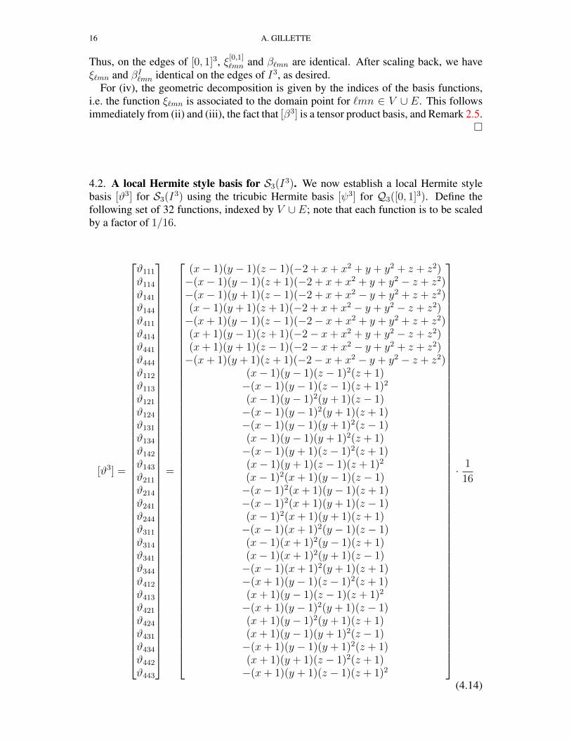
4.2. A local Hermite style basis for S3(I3). We now establish a local Hermite stylebasis [ϑ3] for S3(I3) using the tricubic Hermite basis [ψ3] for Q3([0, 1]3). Define thefollowing set of 32 functions, indexed by V ∪ E; note that each function is to be scaledby a factor of 1/16.

[ϑ3] =

ϑ111

ϑ114

ϑ141

ϑ144

ϑ411

ϑ414

ϑ441

ϑ444

ϑ112

ϑ113

ϑ121

ϑ124

ϑ131

ϑ134

ϑ142

ϑ143

ϑ211

ϑ214

ϑ241

ϑ244

ϑ311

ϑ314

ϑ341

ϑ344

ϑ412

ϑ413

ϑ421

ϑ424

ϑ431

ϑ434

ϑ442

ϑ443

=

(x− 1)(y − 1)(z − 1)(−2 + x+ x2 + y + y2 + z + z2)−(x− 1)(y − 1)(z + 1)(−2 + x+ x2 + y + y2 − z + z2)−(x− 1)(y + 1)(z − 1)(−2 + x+ x2 − y + y2 + z + z2)(x− 1)(y + 1)(z + 1)(−2 + x+ x2 − y + y2 − z + z2)−(x+ 1)(y − 1)(z − 1)(−2− x+ x2 + y + y2 + z + z2)(x+ 1)(y − 1)(z + 1)(−2− x+ x2 + y + y2 − z + z2)(x+ 1)(y + 1)(z − 1)(−2− x+ x2 − y + y2 + z + z2)−(x+ 1)(y + 1)(z + 1)(−2− x+ x2 − y + y2 − z + z2)

(x− 1)(y − 1)(z − 1)2(z + 1)−(x− 1)(y − 1)(z − 1)(z + 1)2

(x− 1)(y − 1)2(y + 1)(z − 1)−(x− 1)(y − 1)2(y + 1)(z + 1)−(x− 1)(y − 1)(y + 1)2(z − 1)(x− 1)(y − 1)(y + 1)2(z + 1)−(x− 1)(y + 1)(z − 1)2(z + 1)(x− 1)(y + 1)(z − 1)(z + 1)2

(x− 1)2(x+ 1)(y − 1)(z − 1)−(x− 1)2(x+ 1)(y − 1)(z + 1)−(x− 1)2(x+ 1)(y + 1)(z − 1)(x− 1)2(x+ 1)(y + 1)(z + 1)−(x− 1)(x+ 1)2(y − 1)(z − 1)(x− 1)(x+ 1)2(y − 1)(z + 1)(x− 1)(x+ 1)2(y + 1)(z − 1)−(x− 1)(x+ 1)2(y + 1)(z + 1)−(x+ 1)(y − 1)(z − 1)2(z + 1)(x+ 1)(y − 1)(z − 1)(z + 1)2

−(x+ 1)(y − 1)2(y + 1)(z − 1)(x+ 1)(y − 1)2(y + 1)(z + 1)(x+ 1)(y − 1)(y + 1)2(z − 1)−(x+ 1)(y − 1)(y + 1)2(z + 1)(x+ 1)(y + 1)(z − 1)2(z + 1)−(x+ 1)(y + 1)(z − 1)(z + 1)2

· 1

16

(4.14)


We fix the following basis orderings, with omitted basis functions ordered lexico-graphically by index.

[ϑ3] := [ ϑ111, . . . , ϑ444︸︷︷︸indices in V

, ϑ112, . . . , ϑ443︸︷︷︸indices in E

], (4.15)

[β] := [ ψ111, . . . , ψ444︸︷︷︸indices in V

, ψ112, . . . , ψ443︸︷︷︸indices in E

, ψ122, . . . , ψ433︸︷︷︸indices in F

, ψ222, . . . , ψ333︸︷︷︸indices in M

, ] (4.16)

Theorem 4.2. Let ψI`mn denote the derivative-preserving scaling of ψ`mn to I3, i.e.

ψI`m := ψ`((x+ 1)/2)ψm((y + 1)/2)ψn((z + 1)/2), `mn ∈ V,

ψI`mn := 2ψ`((x+ 1)/2)ψm((y + 1)/2)ψn((z + 1)/2), `mn ∈ E.

The set [ϑ3] has the following properties:(i) [ϑ3] is a basis for S3(I3).

(ii) [ϑ3] reduces to [ϑ2] on faces of I3.(iii) For any `mn ∈ V ∪ E, ϑ`mn is identical to ψI

`mn on edges of I3.(iv) [ϑ3] is a geometric decomposition of S3(I3).

Proof. The proof is similar to that of Theorem 3.3 so we abbreviate some details. For (i),let [ϑ3][0,1] denote the scaling of [ϑ3] to [0, 1]3. Given the basis orderings in (4.15)-(4.16),we have

[ϑ3][0,1] = W[ψ3] (4.17)where W is the 32× 64 matrix with the structure

W :=[I W′

], (4.18)

where I is the 32× 32 identity matrix and W′ is a specific 32× 32 matrix whose entriesare in {−1, 0, 1}. The matrix W is constructed similarly to the matrix U from the proofof Theorem 4.1; the columns of W satisfy the relationship

εr,iεs,jεt,k =∑

`mn∈V ∪E

εr,iεs,jεt,kw`mnijk , (4.19)

for all (r, s, t) tuples such that sldeg(xryszt) ≤ 3. Similar to previous proofs, this yields

xryszt =∑

`mn∈V ∪E

εr,`εs,mεt,nϑ`mn, (4.20)

proving, after derivative-preserving scaling, that [ϑ3] is a basis for S3(I3).For (ii)-(iv), the proof is similar to the corresponding parts of the proof of Theorem 4.1.

�

5. CONLUCSIONS AND FUTURE DIRECTIONS

The basis functions presented in this work are well-suited for use in both geometricmodeling and finite element applications, as discussed in the introduction. Moreover,the proof techniques used for the theorems suggest a number of promising extensions.Similar techniques should be able to produce Bernstein style bases for higher polynomialorder serendipity spaces, although the introduction of interior degrees of freedom thatoccurs when r > 3 requires some additional care to resolve. Some higher order Hermitestyle bases may also be available, although the association of directional derivative valuesto vertices is somewhat unique to the r = 3 case. Pre-conditioners for finite elementmethods employing our bases are still needed. The fact that all the functions we definedare fixed linear combinations of standard bicubic or tricubic basis functions suggests thatsuch pre-conditioners will have a straightforward construction.

18 A. GILLETTE

REFERENCES

[1] D. Arnold and G. Awanou. The serendipity family of finite elements. Foundations of ComputationalMathematics, 11(3):337–344, 2011.

[2] D. Arnold and G. Awanou. Finite element differential forms on cubical meshes. Arxiv preprintarXiv:1204.2595, 2012.

[3] D. Arnold, R. Falk, and R. Winther. Geometric decompositions and local bases for spaces of fi-nite element differential forms. Computer Methods in Applied Mechanics and Engineering, 198(21-26):1660–1672, 2009.

[4] W. Bangerth, R. Hartmann, and G. Kanschat. deal. ii—a general-purpose object-oriented finite ele-ment library. ACM Transactions on Mathematical Software (TOMS), 33(4):24–es, 2007.

[5] C. Bradley, A. Pullan, and P. Hunter. Geometric modeling of the human torso using cubic hermiteelements. Annals of Biomedical Engineering, 25:96–111, 1997.

[6] P. Ciarlet and P. Raviart. General Lagrange and Hermite interpolation in Rn with applications to finiteelement methods. Archive for Rational Mechanics and Analysis, 46(3):177–199, 1972.

[7] P. G. Ciarlet. The Finite Element Method for Elliptic Problems, volume 40 of Classics in AppliedMathematics. SIAM, Philadelphia, PA, second edition, 2002.

[8] J. Cottrell, T. Hughes, and Y. Bazilevs. Isogeometric analysis: toward integration of CAD and FEA.John Wiley & Sons Inc, 2009.

[9] J. Evans and T. Hughes. Explicit trace inequalities for isogeometric analysis and parametric hexahe-dral finite elements. Numerische Mathematik, pages 1–32, 2011.

[10] T. Hughes. The finite element method. Prentice Hall Inc., Englewood Cliffs, NJ, 1987.[11] J. Mandel. Iterative solvers by substructuring for the p-version finite element method. Computer

Methods in Applied Mechanics and Engineering, 80(1-3):117–128, 1990.[12] M. Mortenson. Geometric Modeling. John Wiley and Sons, 3rd edition, 2006.[13] A. Rand, A. Gillette, and C. Bajaj. Quadratic serendipity finite elements on polygons using general-

ized barycentric coordinates. arXiv:1109.3259, 2011.[14] G. Strang and G. J. Fix. An analysis of the finite element method. Prentice-Hall Inc., Englewood

Cliffs, N. J., 1973.[15] B. Szabo and I. Babuska. Finite element analysis. Wiley-Interscience, 1991.[16] Y. Zhang, X. Liang, J. Ma, Y. Jing, M. J. Gonzales, C. Villongco, A. Krishnamurthy, L. R. Frank,

V. Nigam, P. Stark, S. M. Narayan, and A. D. McCulloch. An atlas-based geometry pipeline forcardiac Hermite model construction and diffusion tensor reorientation. Medical Image Analysis, (inpress), 2012.

E-mail address: [email protected]

DEPARTMENT OF MATHEMATICS, UNIVERSITY OF CALIFORNIA SAN DIEGO, LA JOLLA CA 92093

Documents

HERMITE AND BERNSTEIN STYLE BASIS FUNCTIONS FOR CUBIC SERENDIPITY