Heston-Type Stochastic Volatility with a Markov Switching ... › seminars_events › fileupload › ...Heston-Type Stochastic Volatility with a Markov Switching Regime Robert J. Elliott(a)

Introduction Model Setup Characteristic Function Option Price Numerical Analysis Conclusion References

Heston-Type Stochastic Volatility with aMarkov Switching Regime

Robert J. Elliott(a) Katsumasa Nishide(b) Carlton-James U. Osakwe(c)

(a) University of Adelaide, University of South Australia, University of Calgary

(b) Yokohama National University

(c) Mount Royal University

The full paper is available at http://ssrn.com/abstract=2470975.

http://ssrn.com/abstract=2470975


Plan of Talk

Introduction

Model Setup

Characteristic Function

Option Price

Numerical Analysis

Conclusion


Introduction


Notations

In this talk, we use little letters as scalars, bold letters asn-dimensional vectors, and big letters as n× n matrices:

s price of underlying risky asset,x logarithm of s,v volatility of s,r risk-free rate,k exercise price,τ maturity of option,ei unit vector whose i-th component is one,Γ transition-rate matrix of the regime.


Stochastic Volatility Model

• Smiles and skews in implied volatility.• Local volatility,• Stochastic volatility.

• Heston (1993):Underlying dst/st = rdt+

√vtdw

st ,

Volatility dvt = κ(θ − vt)dt+ σv√vtdw

vt .

The two Brownian motions can be correlated.• Option price is written as

c = c(t, s, v).

• The obtained price formula is semi-analytic, expressedwith the inverse Fourier transform.


Previous studies

• Derman (1999) documents that the slope of volatility smirkis largely independent of the current level of volatility.

• Extensions:• Multi-factor: Christoffersen et al. (2009),• Time-dependent parameters: Benhamou et al. (2010),• Simulation based: Andersen (2008), Fuh et al. (2012).

• Negatively biased.• Numerics of PDE: Chiarella et al. (2009), Chiarella et al.

(2012).• Higher dimension.


Stylized facts• Engle and Patton (2001): Volatility model should have the

properties of• persistence (clustering),• mean reversion.

• Dueker (1997) empirically reports that a Markov switchingSV better fits actual data of the volatility index (VIX).

0

20

40

60

80

20100101 20101231 20111230 20121228 20131227

Volatility Index Japan (VXJ)


Our Model

• Apply Elliott and Osakwe (2006), Elliott et al. (2007) andElliott and Nishide (2014) to price a (plain vanilla) option.

• The mean-reverting level θ is modulated by a Markov chainwith n possible states:

θt ∈ {θ1, . . . , θn}.• θ is independent of zs and zv.• The transition-rate matrix is given by Γ = (γij)

ni,j=1:

γij∆t ≈ P{θt+∆t = θj |θt = θi}for i = j.


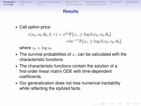
Results

• Call option price:

c(x0, v0, θ0, k, τ) = ex0P{xτ ≥ log k|x0, v0, θ0}+ke−rτP{xτ ≥ log k|x0, v0, θ0}

where xt = log st.• The survival probabilities of xτ can be calculated with the

characteristic functions.• The characteristic functions contain the solution of a

first-order linear matrix ODE with time-dependentcoefficients.

• Our generalization does not lose numerical tractabilitywhile reflecting the stylized facts.


Model Setup


Price dynamics

• The risk-free rate is assumed to be a constant r forsimplicity.

• The price of the underlying asset followsdst/st = rdt+

√vtdw

st

under the risk-neutral measure P.• Let xt = log st. From Ito’s formula, we have

dxt = (r − vt/2)dt+√vtdw

st .


Volatility structure

• The volatility followsdvt = κ(θt − vt)dt+ σv

√vtdw

vt .

under P. We assume that [ws, wv]t = ρt.• The mean-reverting level θt is driven by a Markov chain

with n possible states ϑ = (θ1, . . . , θn)′. The transition-ratematrix is given by Γ.

• If we writezt = (1{θt=θ1}, . . . , 1{θt=θn})

′ ∈ {e1, . . . , en},then θt = ⟨ϑ, zt⟩. Hereafter we call z be the regime vector.

• The dynamics of z is given bydzt = Γ′ztdt+ dmt,

with some n-dimensional vector martingale m.


The problem to solve

• Consider the price of a European call option on the riskyasset with maturity τ and strike price k.

• What we want to get isc(x, v, z, k, τ) = E[e−rτ (exτ − k)+|x0 = x, v0 = v, z0 = z]

• Easily verified that the price can be written asc(x, v, z, k, τ) = exP0{xτ ≥ log k}+ ke−rτP0{xτ ≥ log k}

where P0 is defined byP0(A) = E[e−rτ+(xτ−x)1A|x0 = x, v0 = v, z0 = z]

• Note that the two survival functions are obtained if we havethe characteristic functions of xτ under the probabilitymeasures.


Characteristic Function


Formulation

• Consider the two processes x and v whose dynamics aregiven by

dx = (r + cv)dt+√vdws

t ,dv = (qt − bv)dt+ σv

√vdwv

t ,

where b and c are constants and q(·) is a deterministicfunction.

• Let f(x, v, t) = Et[h(xτ , vτ )] for t < τ . Then, f satisfies thePDF

12vfxx + ρσvvfxv +

12σ

2vvfvv + (r + cv)fx + (qt − bv)fv + ft = 0,

where ft, fx, ... , fvv are partial derivatives. The boundarycondition is f(x, v, τ) = h(x, v).


PDF of the characteristic function

• Take h(x, v) = eiϕx, where ϕ is a constant and i =√−1.

• Following Heston (1993), we conjecturef(x, v, t) = exp{αt + βtv + iϕx},

where α(·) and β(·) are deterministic functions.• Substituting the conjectured function into the PDE, we have

−12vϕ

2f + iϕρσvvβtf + 12σ

2vvβ

2t f

+i(r + cv)ϕf + (qt − bv)βtf + (αt + βtv)f = 0.

• Since the above equation holds for any x and v, we havethe simultaneous ODE

irϕ+ qtβt + αt = 0,

−12ϕ

2 + iϕρσvβt +12σ

2vβ

2t + icϕ− bβt + βt = 0

with ατ = βτ = 0.


Solution of ODEs

• The second ODE is solved as

βt =b− iρσvϕ+ η

σ2v

(1− eη(τ−t)

1− γeη(τ−t)

)where

γ =b− iρσvϕ+ η

b− iρσvϕ− η,

η =√

(b− iρσvϕ)2 + σ2vϕ(ϕ− 2ic).

• The function α is expressed from the first ODE as

αt = irϕ(τ − t) +

∫ τ

tβuqudu.


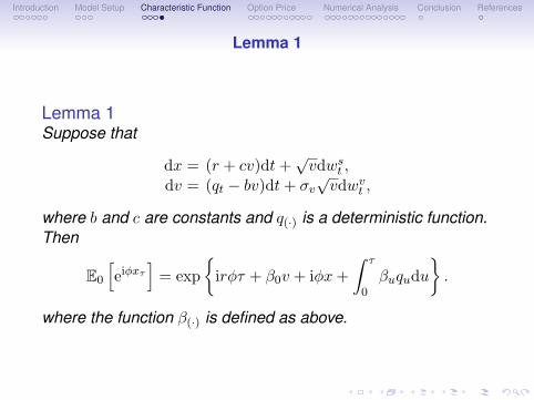
Lemma 1

Lemma 1Suppose that

dx = (r + cv)dt+√vdws

t ,dv = (qt − bv)dt+ σv

√vdwv

t ,

where b and c are constants and q(·) is a deterministic function.Then

E0

[eiϕxτ

]= exp

{irϕτ + β0v + iϕx+

∫ τ

0βuqudu

}.

where the function β(·) is defined as above.


Option Price


Calculation of the survival probability

• WriteFxt = σ{xu; 0 ≤ u ≤ t},

Fvt = σ{vu; 0 ≤ u ≤ t},

Fzt = σ{zu; 0 ≤ u ≤ t}.

• Note that given the information Fzτ , the mean-reverting

level θ = ⟨ϑ, z⟩ can be treated as a deterministic functionof time.

• Again what we want to get isc(x0, v0, z0, k, τ) = ex0P0{xτ ≥ log k}

+ke−rτP0{xτ ≥ log k}where P0 is defined by

P(A) = E[e∫ τ0

√vudzsu− 1

2

∫ τ0 vudu1A

].


Dynamics under P

• We first consider P0{xτ ≥ log k}.• The two processes x and v follow

dx = (r − v/2)dt+√vdws

t ,

dv = κ(θt − v)dt+ σv√vdwv

t ,

under P.• Note that the characteristic function of xτ satisfies

f(ϕ;x0, v0, z0) = E0

[eiϕxτ

]= E0

[E0

[eiϕxτ

∣∣∣Fzτ

]]from the tower property of conditional expectations.


Conditional CF under P

• By setting b = κ, c = −1/2 and qt = κθt = κ⟨ϑ, zt⟩ inLemma 1,

E0

[eiϕxτ

∣∣∣Fzτ

]= exp

{irϕτ + β0v0 + iϕx0 + κ

∫ τ

0βu⟨ϑ, zu⟩du

},

where

βt =κ− iρσvϕ+ η

σ2v

(1− eη(τ−t)

1− γeη(τ−t)

),

γ =κ− iρσvϕ+ η

κ− iρσvϕ− η,

η =√

(κ− iρσvϕ)2 + σ2vϕ(ϕ+ i).

• It suffices to obtain the expectation ofeκ

∫ τ0 βu⟨ϑ,zu⟩du

to derive the unconditional characteristic function.


Auxiliary process

• Consider the scalar process

gt = exp

{κ

∫ t

0βu⟨ϑ, zu⟩du

}and the vector process gt = gtzt.

• The vector process g follows

dgt = gtdzt + ztdgt

= gt(Γ′ztdt+ dmt) + κβt⟨ϑ, zt⟩gtztdt

= (Γ′ + κβtΘ)gtztdt+ gtdmt

where Θ = diag[ϑ].


Matrix ODE

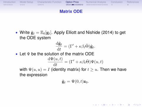
• Write gt = E0[gt]. Apply Elliott and Nishide (2014) to getthe ODE system

dgtdt

= (Γ′ + κβtΘ)gt.

• Let Ψ be the solution of the matrix ODEdΨ(u, t)

dt= (Γ′ + κβtΘ)Ψ(u, t)

with Ψ(u, u) = I (identity matrix) for t ≥ u. Then we havethe expression

gt = Ψ(0, t)z0.


Final form of the survival function

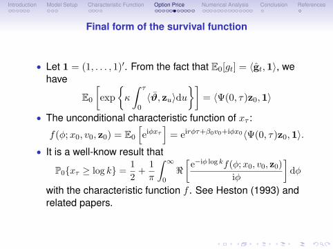
• Let 1 = (1, . . . , 1)′. From the fact that E0[gt] = ⟨gt,1⟩, wehave

E0

[exp

{κ

∫ τ

0⟨ϑ, zu⟩du

}]= ⟨Ψ(0, τ)z0,1⟩

• The unconditional characteristic function of xτ :

f(ϕ;x0, v0, z0) = E0

[eiϕxτ

]= eirϕτ+β0v0+iϕx0⟨Ψ(0, τ)z0,1⟩.

• It is a well-know result that

P0{xτ ≥ log k} =1

2+

1

π

∫ ∞

0ℜ[e−iϕ log kf(ϕ;x0, v0, z0)

iϕ

]dϕ

with the characteristic function f . See Heston (1993) andrelated papers.


Dynamics under P

• We next consider P0{xτ ≥ log k}, or

E0

[eiϕxτ

]= E0

[e∫ τ0

√vudzsu− 1

2

∫ τ0 vudu × eiϕxτ

]• From the Girsanov theorem, we have

dx = (r + v/2)dt+√vdws,

dv = (κθt − (κ− ρσv)v)dt+ σv√vdwv.

with some P-Brownian motions ws and wv. Here thecorrelation remains the same, i.e., [ws, wv]t = ρt.

• We can directly apply the lemma by settingb = κ− ρσv,c = 1/2,qt = κθt = κ⟨ϑ, zt⟩.


Lemma 2

Lemma 2

E0

[eκ

∫ τ0 βuθudu

]= E0

[eκ

∫ τ0 βuθudu

]where β is a deterministic function of time.

Proof.

E0

[eκ

∫ τ0 βuθudu

]= E0

[e∫ τ0

√vudzsu− 1

2

∫ τ0 vudu × eκ

∫ τ0 βuθudu

]= E0

[E0

[e∫ τ0

√vudzsu− 1

2

∫ τ0 vudu

∣∣∣Fzτ

]eκ

∫ τ0 βuθudu

]= E0

[eκ

∫ τ0 βuθudu

].


Option price formula

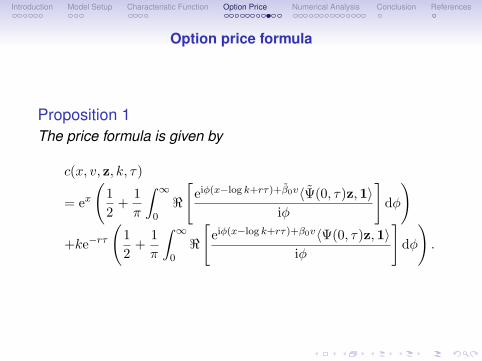
Proposition 1The price formula is given by

c(x, v, z, k, τ)

= ex

(1

2+

1

π

∫ ∞

0ℜ

[eiϕ(x−log k+rτ)+β0v⟨Ψ(0, τ)z,1⟩

iϕ

]dϕ

)

+ke−rτ

(1

2+

1

π

∫ ∞

0ℜ

[eiϕ(x−log k+rτ)+β0v⟨Ψ(0, τ)z,1⟩

iϕ

]dϕ

).


Option price formula (cont’d)

Proposition 1 (cont’d)Here β and Ψ are defined as above, and

βt =κ− ρσv − iρσvϕ+ η

σ2v

(1− eη(τ−t)

1− γeη(τ−t)

)γ =

κ− ρσv − iρσvϕ+ η

κ− ρσv − iρσvϕ− η,

η =√

(κ− ρσv − iρσvϕ)2 + σ2vϕ(ϕ− i)

and the matrix Ψ is the solution of the ODE

dΨ(u, t)

dt=(Γ′ + κβtΘ

)Ψ(u, t)

with Ψ(u, u) = I.


Unobservable regime

Remark 1Suppose that θ is unobservable but its probability is estimatedand updated by the information. Then the price of a call optionis equal to

n∑j=1

P0{θ0 = θj}c(x, v, ej , k, τ).

Thus our pricing formula is still useful in the case where theregime is unobservable.


Numerical Analysis


Numerical analysis

• We assume two-state Markov switching for simplicity.• Basecase parameters:

s0 r ρ σv κ θ1 θ2 γ12 γ21

100 .05 −.5 .2 1.5 .025 .075 .5 1.

• θ1: low regime• θ2: high regime

• Compare option prices by the analytical formula with theones generated from Monte Carlo simulations.


Case 1; low vol. and low regime

v0 = .02 < θ0 = θ1 < θ2

Maturityk 3 Months 6 Months 9 Months 12 Months

90 11.3319 13.0306 14.8427 16.6474(-.0725) (-.5192) (-.8235) (-.9728)

95 6.9447 9.0492 11.1387 13.1456(-.3561) (-.9653) (-1.2012) (-1.3623)

100 3.5131 5.8249 8.0431 10.1464(-.5809) (-1.2186) (-1.4543) (-1.6242)

105 1.7008 3.6663 5.7120 7.7363(-.2722) (-1.0579) (-1.4471) (-1.6022)

110 0.8419 2.4352 4.1305 5.9219(.0409) (-.5892) (-1.1381) (-1.4440)


Case 1: volatility surface

3

6

9

12

0.14

0.16

0.18

0.20

0.22

0.24

0.26

90

95

100

105

110

vo

lati

lity

strike price

maturity


Case 2; low vol. and high regime

v0 = .02 < θ1 < θ0 = θ2


90 11.4947 13.8235 16.0228 18.0065(.0684) (.2255) (.3488) (.3247)

95 7.4890 10.3224 12.7494 14.8714(.1918) (.2432) (.3598) (.4435)

100 4.5036 7.4961 9.9917 12.1618(.3740) (.4415) (.4238) (.3951)

105 2.7005 5.3886 7.7693 9.8884(.7026) (.6241) (.6134) (.6006)

110 1.7059 3.9083 6.0433 8.0263(.8736) (.8778) (.7829) (.6299)



3

6

9

12

0.14

0.16

0.18

0.20

0.22

0.24

0.26

90

95

100

105

110

vo

lati

lity

strike price

maturity


Case 3; intermediate vol. and low regime

θ0 = θ1 < v0 = .05 < θ2


90 11.8715 13.7797 15.5899 17.3374(-.0205) (-.4481) (-.7805) (-.8870)

95 7.9074 10.0973 12.0915 13.9854(-.1687) (-.7256) (-1.0294) (-1.2299)

100 4.7468 7.0427 9.1159 11.0762(-.3146) (-.9578) (-1.1777) (-1.3685)

105 2.5894 4.7302 6.7327 8.6596(-.3401) (-.9819) (-1.3293) (-1.4629)

110 1.3359 3.1338 4.9355 6.7321(-.2282) (-.8029) (-1.2256) (-1.4450)



3

6

9

12

0.20

0.22

0.24

0.26

0.28

90

95

100

105

110

vo

lati

lity

strike price

maturity


Case 4; intermediate vol. and high regime

θ1 < v0 = .05 < θ0 = θ2


90 12.1182 14.5487 16.6998 18.6188(.1906) (.3424) (.3157) (.3772)

95 8.3961 11.1920 13.5221 15.5562(.3051) (.3498) (.4647) (.3172)

100 5.4814 8.4089 10.8033 12.8835(.3827) (.4461) (.4065) (.4805)

105 3.4412 6.2186 8.5512 10.6027(.4767) (.5382) (.4888) (.4679)

110 2.1365 4.5712 6.7382 8.6954(.5768) (.6355) (.5923) (.5449)



3

6

9

12

0.20

0.22

0.24

0.26

0.28

90

95

100

105

110

vo

lati

lity

strike price

maturity


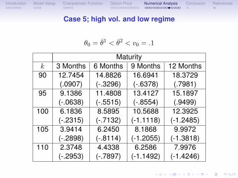
Case 5; high vol. and low regime

θ0 = θ1 < θ2 < v0 = .1


90 12.7454 14.8826 16.6941 18.3729(.0907) (-.3296) (-.6378) (.7981)

95 9.1386 11.4808 13.4127 15.1897(-.0638) (-.5515) (-.8554) (.9499)

100 6.1836 8.5895 10.5688 12.3925(-.2315) (-.7132) (-1.1118) (-1.2485)

105 3.9414 6.2450 8.1868 9.9972(-.2898) (-.8114) (-1.2055) (-1.3818)

110 2.3748 4.4338 6.2586 7.9976(-.2953) (-.7897) (-1.1492) (-1.4246)



3

6

9

12

0.24

0.26

0.28

0.30

0.32

90

95

100

105

110

vo

lati

lity

strike price

maturity


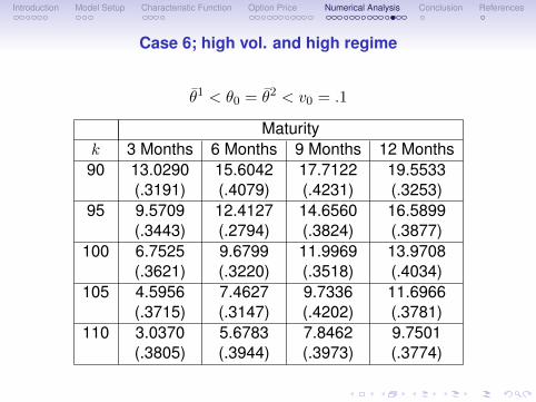
Case 6; high vol. and high regime

θ1 < θ0 = θ2 < v0 = .1


90 13.0290 15.6042 17.7122 19.5533(.3191) (.4079) (.4231) (.3253)

95 9.5709 12.4127 14.6560 16.5899(.3443) (.2794) (.3824) (.3877)

100 6.7525 9.6799 11.9969 13.9708(.3621) (.3220) (.3518) (.4034)

105 4.5956 7.4627 9.7336 11.6966(.3715) (.3147) (.4202) (.3781)

110 3.0370 5.6783 7.8462 9.7501(.3805) (.3944) (.3973) (.3774)



3

6

9

12

0.24

0.26

0.28

0.30

0.32

90

95

100

105

110

vo

lati

lity

strike price

maturity


Model Implications

• A wide variety of volatility surfaces are obtained.• Option prices calculated with analytic formula tend to be

lower (resp. higher) than those by Monte Carlo simulationsin the low (resp. high) regime.


Conclusion


Conclusion

• Introduce a Markov switching regime to the Heston-typestochastic volatility models.

• The characteristic function of the log price containssolutions of simple matrix ODEs.

• Captures stylized facts while not losing mathematicaltractability.

• Future works:• Credit products.


References I

[1] Andersen, L. (2008), "Simple and Efficient Simulation of the HestonStochastic Volatility Model", Journal of Computational Finance, 11(3),1–42.

[2] Benhamou, E., F. Gebet and M. Miri (2010), "Time Dependent HestonModel", SIAM Journal of Financial Mathematics, 1(1), 289–325.

[3] Chiarella, C., B. Kang, G.H. Meyer and A. Ziogas (2009), "TheEvaluation of American Option Prices under Stochastic Volatility andJump-Diffusion Dynamics Using the Method of Lines", InternationalJournal of Theoretical and Applied Finance, 12(3), 393–425.

[4] Chiarella, C., B. Kang and G.H. Meyer (2012), "The Evaluation of BarrierOption Prices under Stochastic Volatility", Computers and Mathematicswith Applications, 64(6), 2034–2048.

[5] Christoffersen, P., S. Heston and K. Jacobs (2009), "The Shape andTerm Structure of the Index Option Smirk: Why Multifactor StochasticVolatility Models Work So Well", Management Science, 55(12),1914–1932.

[6] Derman, E. (1999), "Regimes of Volatility", Risk Magazine, 12(4), 55–59.


References II

[7] Engle, R.F. and A.J. Patton (2001), "What Good Is a Volatility Model?",Quantative Finance, 1(2), 237–245.

[8] Elliott, R.J. and K. Nishide (2014), "Pricing of Discount Bonds with aMarkov Switching Regime", Annals of Finance, 10(3), 509–522.

[9] Elliott, R.J. and C.-J.U. Osakwe (2006), "Option Price for a Pure JumpProcesses with Markov Switching Compensators", Finance andStochastics, 10(2), 250–275.

[10] Elliott, R.J., T.K. Siu and L. Chan (2007), "Pricing Volatility Swaps underHeston’s Stochastic Volatility Model with Regime Switching", AppliedMathematical Finance, 14(1), 41–62.

[11] Fuh, C.-D., K.W.R. Ho, I. Hu and R.-H. Wang (2012), "Option Pricingwith Markov Switching", Journal of Data Science, 10(3), 483–509.

[12] Heston, S.L. (1993), "A Closed-Form Solution for Options withStochastic Volatility with Applications to Bond and Currency Options",Review of Financial Studies, 6(2), 327–343.


Thank you for your attention

Documents

Heston-Type Stochastic Volatility with a Markov Switching ... › seminars_events › fileupload › ...Heston-Type Stochastic Volatility with a Markov Switching Regime Robert J. Elliott(a)