Embed Size (px)
Citation preview

Heterogeneous Network Analysis on Academic
Collaboration Networks
A Thesis Submitted for the Degree of
Doctor of Philosophy
By
Qinxue Meng
in
School of Software
UNIVERSITY OF TECHNOLOGY, SYDNEY
AUSTRALIA
JULY 2014
c© Copyright by Qinxue Meng, 2014

UNIVERSITY OF TECHNOLOGY, SYDNEY
SCHOOL OF SOFTWARE
The undersigned hereby certify that they have read this
thesis entitled “Heterogeneous Network Analysis on Academic
Collaboration Networks” byQinxue Meng and that in their opinions
it is fully adequate, in scope and in quality, as a thesis for the degree of
Doctor of Philosophy.
Dated: July 2014
Research Supervisors:Paul J. Kennedy
ii

CERTIFICATE
Date: July 2014
Author: Qinxue Meng
Title: Heterogeneous Network Analysis on Academic
Collaboration Networks
Degree: Ph.D.
I certify that this thesis has not already been submitted for any degreeand is not being submitted as part of candidature for any other degree.
I also certify that the thesis has been written by me and that any help
that I have received in preparing this thesis, and all sources used, have been
acknowledged in this thesis.
Signature of Author
iii

Acknowledgements
I would like to express my gratitude to my supervisor, Paul J. Kennedy
for his continuous encouragement, advice, help and invaluable suggestions to
my study and my life. He is such a nice, generous, helpful and kindhearted
person. At the beginning of my study, it is he who held a series of lectures in
lab meetings covering the fundamental knowledge of research such as common
methods and tools in data mining, writing in Latex and explaining doctoral
framework. During my study at UTS, he builds a relaxing, comfortable and
active environment and I owe my research achievements to his experienced
supervision.
Many thanks go to my lab mates Ahmad Al-oqaily, Hamid Ghous, Siamak
Tafavogh, Hooman Homayoonfard and Ali Anaissi. The discussions with them
in lab meetings are extremely useful to my research and inspire my research. I
appreciate the travel support for attending the international conferences which
I received from the School of Software and QCIS Lab.
I also would like to thank my wife, Wang Wenjun, for her understanding,
assistance and company during my study in Australia. I also thank my parents
for the support of my overseas study. This thesis could not have been completed
without their supports.
Last but not least, special thanks are given to UTS Research & Innovation
Office for providing raw datasets for my research.
Wish you all every success in the future.
iv
Table of Contents
Table of Contents vii
List of Figures 1
List of Tables 4
Abstract 6
Table of Symbols 11
1 Introduction 14
1.1 What are heterogeneous networks? . . . . . . . . . . . . . . . . . . . 16
1.2 Significance of mining heterogeneous networks . . . . . . . . . . . . . 20
1.3 Why study academic collaboration? . . . . . . . . . . . . . . . . . . . 21
1.4 Research questions . . . . . . . . . . . . . . . . . . . . . . . . . . . . 23
1.5 Contributions to knowledge . . . . . . . . . . . . . . . . . . . . . . . 25
1.6 Organisation of contents . . . . . . . . . . . . . . . . . . . . . . . . . 27
2 Literature review 30
2.1 Similarity measures in networks . . . . . . . . . . . . . . . . . . . . . 33
2.1.1 Distance-based similarity measures . . . . . . . . . . . . . . . 33
2.1.2 Neighborhood-based similarity measures . . . . . . . . . . . . 35
2.1.3 Probability-based similarity measures . . . . . . . . . . . . . . 38
2.2 Community detection . . . . . . . . . . . . . . . . . . . . . . . . . . . 39
2.2.1 Similarity-based community detection . . . . . . . . . . . . . . 41
2.2.2 Hierarchical clustering . . . . . . . . . . . . . . . . . . . . . . 44
2.2.3 Spectral-based clustering algorithms . . . . . . . . . . . . . . 46
2.2.4 Modularity partitioning . . . . . . . . . . . . . . . . . . . . . 51
2.2.5 Other community detection methods on heterogeneous networks 53
v

2.2.6 Community detection validation . . . . . . . . . . . . . . . . . 54
2.3 Determining the number of clusters . . . . . . . . . . . . . . . . . . . 58
2.3.1 Clustering result-based methods . . . . . . . . . . . . . . . . . 58
2.3.2 Topological feature-based methods . . . . . . . . . . . . . . . 59
2.3.3 Support Vector Machine (SVM) . . . . . . . . . . . . . . . . . 63
2.4 Link prediction . . . . . . . . . . . . . . . . . . . . . . . . . . . . . . 64
2.5 Ranking . . . . . . . . . . . . . . . . . . . . . . . . . . . . . . . . . . 67
2.6 Research gaps . . . . . . . . . . . . . . . . . . . . . . . . . . . . . . . 69
3 Community detection on heterogeneous networks 71
3.1 Methodology . . . . . . . . . . . . . . . . . . . . . . . . . . . . . . . 72
3.1.1 Multiple semantic-path clustering . . . . . . . . . . . . . . . . 72
3.1.2 Semantic path assessment . . . . . . . . . . . . . . . . . . . . 75
3.2 Clustering evaluation . . . . . . . . . . . . . . . . . . . . . . . . . . . 76
3.2.1 Cluster comparison . . . . . . . . . . . . . . . . . . . . . . . . 76
3.2.2 Cluster validation . . . . . . . . . . . . . . . . . . . . . . . . . 78
3.3 Experimental dataset . . . . . . . . . . . . . . . . . . . . . . . . . . . 78
3.4 Experimental results . . . . . . . . . . . . . . . . . . . . . . . . . . . 81
3.4.1 Collective similarity calculation . . . . . . . . . . . . . . . . . 81
3.4.2 Path assessment . . . . . . . . . . . . . . . . . . . . . . . . . . 83
3.4.3 Community detection and validation . . . . . . . . . . . . . . 87
3.5 Contribution and discussion . . . . . . . . . . . . . . . . . . . . . . . 89
4 Determine the number of clusters by leaders 91
4.1 Leader detection and grouping clustering . . . . . . . . . . . . . . . . 93
4.1.1 Leader identification . . . . . . . . . . . . . . . . . . . . . . . 93
4.1.2 Leader group formation . . . . . . . . . . . . . . . . . . . . . 96
4.1.3 Community detection . . . . . . . . . . . . . . . . . . . . . . . 99
4.2 Clustering validation . . . . . . . . . . . . . . . . . . . . . . . . . . . 100
4.3 Experimental dataset . . . . . . . . . . . . . . . . . . . . . . . . . . . 101
4.4 Experiment . . . . . . . . . . . . . . . . . . . . . . . . . . . . . . . . 102
4.4.1 Leader identification . . . . . . . . . . . . . . . . . . . . . . . 102
4.4.2 Community detection . . . . . . . . . . . . . . . . . . . . . . . 105
4.5 Contribution and discussion . . . . . . . . . . . . . . . . . . . . . . . 107
5 Network evolution-based link prediction 110
5.1 Methodology . . . . . . . . . . . . . . . . . . . . . . . . . . . . . . . 112
5.1.1 Modeling vertex activeness . . . . . . . . . . . . . . . . . . . . 112
5.1.2 Network Evolution-based link prediction . . . . . . . . . . . . 115
vi

5.1.3 Evaluation . . . . . . . . . . . . . . . . . . . . . . . . . . . . . 117
5.2 Experimental dataset . . . . . . . . . . . . . . . . . . . . . . . . . . . 118
5.3 Experimental results . . . . . . . . . . . . . . . . . . . . . . . . . . . 119
5.3.1 Modeling vertex activeness evolution . . . . . . . . . . . . . . 119
5.3.2 Determining vertex evolving patterns . . . . . . . . . . . . . . 120
5.3.3 Link prediction . . . . . . . . . . . . . . . . . . . . . . . . . . 120
5.4 Contribution and discussion . . . . . . . . . . . . . . . . . . . . . . . 122
6 Co-ranking on complex bipartite heterogeneous networks 124
6.1 Data model . . . . . . . . . . . . . . . . . . . . . . . . . . . . . . . . 125
6.1.1 Network model . . . . . . . . . . . . . . . . . . . . . . . . . . 125
6.1.2 Matrix model . . . . . . . . . . . . . . . . . . . . . . . . . . . 126
6.2 Methodology . . . . . . . . . . . . . . . . . . . . . . . . . . . . . . . 127
6.2.1 Ranking based on rules . . . . . . . . . . . . . . . . . . . . . . 127
6.2.2 The co-ranking framework . . . . . . . . . . . . . . . . . . . . 128
6.2.3 Evaluation . . . . . . . . . . . . . . . . . . . . . . . . . . . . . 130
6.3 Experimental dataset . . . . . . . . . . . . . . . . . . . . . . . . . . . 132
6.4 Experiment . . . . . . . . . . . . . . . . . . . . . . . . . . . . . . . . 134
6.4.1 Extracting ranking rules . . . . . . . . . . . . . . . . . . . . . 134
6.4.2 Co-ranking authors and publications . . . . . . . . . . . . . . 138
6.4.3 Evaluation . . . . . . . . . . . . . . . . . . . . . . . . . . . . . 141
6.4.4 Divergence analysis . . . . . . . . . . . . . . . . . . . . . . . . 142
6.5 Contribution and discussion . . . . . . . . . . . . . . . . . . . . . . . 143
7 Conclusions 146
7.1 Future research directions . . . . . . . . . . . . . . . . . . . . . . . . 151
vii

List of Figures
1.1 An example of how to decompose complex heterogeneous networks . . 17
2.1 A simple example of community detection to show that three commu-
nities have been found. . . . . . . . . . . . . . . . . . . . . . . . . . . 40
2.2 An example of hierarchical tree. Horizontal cuts correspond to parti-
tions of a network in communities from Newman & Girvan (2004). . . 44
2.3 An example of graph partitioning. . . . . . . . . . . . . . . . . . . . 47
2.4 Scree graph . . . . . . . . . . . . . . . . . . . . . . . . . . . . . . . . 60
2.5 SVM aims to draw a boundary among objects and those objects in the
same side are classified into one cluster (Cortes & Vapnik 1995). . . . 63
3.1 Examples of semantic paths. . . . . . . . . . . . . . . . . . . . . . . . 73
3.2 The constitution of Field of Research (FoR) codes . . . . . . . . . . . 78
3.3 The schema of the network presenting the academic collaboration at
UTS . . . . . . . . . . . . . . . . . . . . . . . . . . . . . . . . . . . . 80
3.4 Semantic paths derived from the academic collaboration heterogeneous
networks. . . . . . . . . . . . . . . . . . . . . . . . . . . . . . . . . . 82
3.5 The similarity graph of researchers in Scenario I . . . . . . . . . . . . 84
3.6 The similarity graph of researchers in Scenario II . . . . . . . . . . . 85
1

2
3.7 Some laboratories are labeled in the researcher similarity network of
Scenario III. . . . . . . . . . . . . . . . . . . . . . . . . . . . . . . . . 86
4.1 An example of why leaders should be grouped . . . . . . . . . . . . . 97
4.2 The working process of community detection by Leader Detection and
Grouping Clustering. Circles are vertices and LGi refers to leader
groups. The similarity between vertices and leader groups are calcu-
lated and vertices are allocated to those leader groups with highest
similarity. . . . . . . . . . . . . . . . . . . . . . . . . . . . . . . . . . 98
4.3 The schema of the experimental heterogeneous network. . . . . . . . 102
4.4 The distribution of researcher degree centrality . . . . . . . . . . . . 103
4.5 The distribution of researcher betweenness centrality . . . . . . . . . 103
4.6 The result of leader detection by SVM in R. Triangles and circles are
data points from two clusters. Circles stand for leaders and triangles
are community members. Solid triangles and circles are support vectors
of these two clusters respectively. . . . . . . . . . . . . . . . . . . . . 104
4.7 The eigenvalues of the random-walk Laplacian matrix. . . . . . . . . 106
5.1 The schema of the heterogeneous academic collaboration network at
UTS. . . . . . . . . . . . . . . . . . . . . . . . . . . . . . . . . . . . . 118
6.1 An example of a complex bipartite heterogeneous network is used for
co-ranking. . . . . . . . . . . . . . . . . . . . . . . . . . . . . . . . . . 126
6.2 The working flow between different rules in the co-ranking method. . 129
6.3 The data sources of the experimental dataset. . . . . . . . . . . . . . 132

3
6.4 The schema of the experimental complex bipartite heterogeneous net-
work built from the DBLP website. . . . . . . . . . . . . . . . . . . 135
6.5 The academic collaboration network is represented by a matrix for
further computation. . . . . . . . . . . . . . . . . . . . . . . . . . . . 136
6.6 Mutual improvement of co–ranking publications and authors through
iterations. Each of the six pairs of graphs shows the distributions of
publication and author ranks. The x axis in each diagram is ranking
score and the y axis is the frequency of objects. . . . . . . . . . . . . 138
6.7 Convergence analysis: the rates of convergence from the proposed co–
ranking method, PageRank and HITS are illustrated: (a) describes
the process of publication ranking by co–ranking and PageRank; (b)
compares the converge rate between coranking and HITS for author
ranking. . . . . . . . . . . . . . . . . . . . . . . . . . . . . . . . . . . 143

List of Tables
2.1 Summarization of Neighborhood-based similarity measures . . . . . . 35
2.2 Laplacian matrices . . . . . . . . . . . . . . . . . . . . . . . . . . . . 48
3.1 The number of records in files from 2009 to 2011 . . . . . . . . . . . . 80
3.2 Similarity calculation of all semantic paths related to researchers. . . 82
3.3 The paths and their corresponding scalars . . . . . . . . . . . . . . . 83
3.4 Clustering validation . . . . . . . . . . . . . . . . . . . . . . . . . . . 88
3.5 Clustering quality validation . . . . . . . . . . . . . . . . . . . . . . . 89
4.1 A sample of new built dataset . . . . . . . . . . . . . . . . . . . . . . 95
4.2 The number of records in files from 2009 to 2011 . . . . . . . . . . . . 101
4.3 Clustering results by spectral clustering . . . . . . . . . . . . . . . . . 106
4.4 Clustering results by spectral clustering and LDGC . . . . . . . . . . 107
5.1 The experimental dataset from UTS . . . . . . . . . . . . . . . . . . 118
5.2 Statistics of the academic collaboration network from 2006 to 2011 . . 119
5.3 Categories of vertices . . . . . . . . . . . . . . . . . . . . . . . . . . 120
5.4 Link prediction accuracy comparison. . . . . . . . . . . . . . . . . . 121
6.1 Statistics of the academic network used to validate the proposed co-
ranking approach . . . . . . . . . . . . . . . . . . . . . . . . . . . . . 133
4

5
6.2 Top 10 authors and publications by co–ranking . . . . . . . . . . . . 140
6.3 Top 10 authors by co–ranking and their H-index scores by CiteSeer . 141
6.4 Evaluation of ranking results by co–ranking, PageRank and HITS . . 142

Abstract
Heterogeneous networks are a type of complex network model which can have multi-
type objects and relationships. Nowadays, research on heterogeneous networks has
been increasingly attracting interest because these networks are more advantageous
in modeling real-world situations than traditional networks, that is homogenous net-
works, that can only have one type of object and relationship. For example, the
network of Facebook has vertices including photographs, companies, movies, news
and messages and different relationships among these objects. Besides that, hetero-
geneous networks are especially useful for representing complex abstract concepts,
such as friendship and academic collaboration. Because these concepts are hard to
measure directly, heterogeneous networks are able to represent these abstract concepts
by concrete and measurable objects and relationships. Because of these features, het-
erogeneous networks are applied in many areas including social networks, the World
Wide Web, research publication networks and so on. This motivates the thesis to
work on network analysis in the context of heterogeneous networks.
In the past, homogeneous networks were the research focus of network analysis
and therefore many methods proposed by previous studies for social network analy-
sis were designed for homogenous networks. Although heterogeneous networks can
be considered as an extension of homogenous networks, most of these methods are
6

Abstract 7
not applicable on heterogeneous networks because these methods can only address
one type of object and relationships instead of dealing with multi-type ones. In net-
work analysis, there are three basic problems including community detection, link
prediction and object ranking. These three questions are the basis of many practical
questions, such as network structure extraction, recommendation systems and search
engines. Community detection, also called clustering, aims to find the community
structure of a network including subgroups of vertices that are closely related, which
can facilitate people to understand the structure of networks. Link prediction is a
task for finding links which are currently non-existent in networks but may appear
in the future. Object ranking can be viewed as an object evaluation task which aims
to order a set of objects based on their importance, relevance, or other user defined
criteria. In addition to these three research issues, approaches for determining the
number of clusters a priori is also important because it can improve the quality of
community detection significantly. This thesis works on heterogeneous network and
proposes a set of methods to address the four main research problems in network
analysis including community detection, determining the number of clusters, link
prediction and object ranking.
There are four contributions in this thesis. Contribution 1 proposes a Multiple
Semantic-path Clustering method which can facilitate users to achieve a desired clus-
tering in heterogeneous networks. Contribution 2 develops a Leader Detection and
Grouping Clustering method which can determine the number of clusters a priori,
thereby improving the quality of clustering. Contribution 3 introduces a Network
Evolution-based Link Prediction method which can improve link prediction accuracy
by modeling evolution patterns of objects. Contribution 4 proposes a co-ranking

Abstract 8
method which can work on complex bipartite heterogeneous networks where one type
of vertex can connect to themselves directly and indirectly.
The performance of all developed methods in the thesis in terms of clustering
quality, link prediction accuracy and ranking effectiveness, is evaluated in the con-
text of a research management dataset of University of Technology, Sydney (UTS)
and public bibliographic DBLP (DataBase systems and Logic Programming) dataset.
Moreover, all the results of the proposed methods in this thesis are compared with
state-of-the-art methods and these experimental results suggest that the proposed
methods outperform these state-of-the-art methods in quantitative and qualitative
analysis.

Publications 9
Publications
Below is the list of the journal and conference papers associated with my PhD re-
search:
1. Meng, Q., Tafavogh, S. & Kennedy, P. J. (2014), ‘Community Detection on
Heterogeneous Networks by Multiple Semantic-Path Clustering’, in ‘Proceed-
ings of the 6th International Conference on Computational Aspects of Social
Networks (CASoN)’, IEEE.
2. Tafavogh, S., Meng, Q., Catchpoole, D. R., Kennedy, P. J. (2014), ‘Automated
quantitative and qualitative analysis of the whole slide images of neuroblastoma
tumor for making a prognosis decision’, in ‘Proceedings of The 11th IASTED
International Conference on Biomedical Engineering (BioMed 2014)’, IEEE.
3. Asabere, N. Y., Xia, F., Meng, Q., Li, F. & Liua, H. (2014), ‘Scholarly pa-
per recommendation based on social awareness and folksonomy’, International
Journal of Parallel, Emergent and Distributed Systems.
4. Meng, Q. & Kennedy, P. J. (2013b), ‘Survey on spectral clustering and its appli-
cations in social networks’, Computer Engineering and Applications 49(3), 213–
221.
5. Meng, Q. & Kennedy, P. J. (2013a), ‘Discovering influential authors in het-
erogeneous academic networks by a co-ranking method’, in ‘Proceedings of the
22nd ACM International Conference on Information & Knowledge Manage-
ment’, ACM, pp. 1029–1036.

Publications 10
6. Meng, Q. & Kennedy, P. J. (2012c), ‘Using network evolution theory and sin-
gular value decomposition method to improve accuracy of link prediction in
social networks’, in ‘Proceedings of the Tenth Australasian Data Mining Con-
ference’,Volume 134, Australian Computer Society, Inc., pp. 175–181.
7. Meng, Q. & Kennedy, P. J. (2012b), ‘Using field of research codes to discover
research groups from co-authorship networks’, in ‘Proceedings of the 2012 In-
ternational Conference on Advances in Social Networks Analysis and Mining
(ASONAM 2012)’, IEEE Computer Society, pp. 289–293.
8. Meng, Q. & Kennedy, P. J. (2012a), ‘Determining the number of clusters in
co-authorship networks using social network theory’, in ‘2012 Second Inter-
national Conference on Social Computing and Its Applications (SCA 2012)’,
IEEE, pp. 337–343.

Table of Symbols
Symbols Description
G Networks or graphs
V Vertex set
|V | the number of vertices
E Edge set
|E| the number of edges
P Semantic path set
|P | the number of semantic paths
Vn The set of vertices in type n
Em The set of edges in type m
v, u vertices
euv The edge from vertex u to v
A Adjacency matrix
auv An element of adjacency matrix A.
If auv = 1, there is an edge from u and v;
If auv = 0, vertex u and v are not connected.
11

Table of Symbols 12
Symbols Description
W Weighted adjacency matrix
wuv the weight of edge euv
dv Degree of vertex v, dv =∑|V |
i=1wvi
D Degree matrix which is a diagonal matrix
with the degrees d1, . . . , d|V |
L Laplacian matrix
li ith eigenvalue of Laplacian matrix
I Identify matrix
S Similarity matrix
suv The similarity beween vertex u and v
C Cluster indicator matrix
k Number of clusters
W ViVj The weight adjacency matrix
between object type Vi and Vj
wViVjuv w
ViVjuv = wuv where u ∈ Vi and v ∈ Vj
CD Vertex degree centrality
CB Vertex betweenness centrality
LGi ith leader group

Table of Symbols 13
Symbols Description
Nuv(i) The number of paths between vertex u and v
and that belong to semantic path i
len(i) The length of semantic path i
X, Y Network partitions
T (u, v) Time of randomly moving agent from
starting vertex u to the end vertex v
Ω Network evolution
neighor(v, t) The neighborhood set of vertex v in timeslot t
rank(v, i) The ranking scores of vertex v in ith iteration
Diff(i, i+ 1) The difference of vertex ranking scores
between ith iteration and (i+ 1)th iteration

Chapter 1
Introduction
The world where we are living is interconnected and interrelated: most data such
as objects, groups or components link or interact with each other, thereby forming
numerous, large, interconnected and complex networks. As a result, the analysis of
large-scale, complex networks has gained wide attention nowadays from researchers
in computer science, social science, physics, economics, biology, and so on. This is not
only because network analysis can facilitate people to understand how current net-
works are formed but also because the research can forecast the direction of network
evolution and identify the roles networked objects play.
Recently the advent of Web 2.0 and advances in mobile technologies have acceler-
ated information publishing, sharing, interaction and collaboration across the world,
making the process of collecting, integrating and organising data much easier than
ever before. This drives the emergence and rapid growth of many successful online so-
cial, academic, and information sharing networks. Most of those real-world networks
are heterogeneous, where vertices and relations are of different types (Sun & Han
2012). For example, in academic networks, vertices can be researchers, publications,
14

Chapter 1. Introduction 15
venues, and so on. Clearly, treating all the vertices as the same type is unreason-
able as different vertices have different patterns in forming networks and in network
evolution. Thus heterogeneous network modelling is needed to capture the essential
information of those networks.
Till now the theories and methods related to network analysis have been well
researched via both theoretical and experimental studies. However, most current
network analysis research (Scott & Carrington 2011) is based on homogeneous net-
works where vertices are objects of the same entity type (e.g., authors) and links
are relationships from the same relation type (e.g., co-authorship). Most famous
and widely applied network analysis methods are based on homogeneous networks,
such as neighbourhood theory (Lu & Zhou 2011), Katz similarity (Katz 1953), ran-
dom walk (Spitzer 2001), spectral clustering (von Luxburg 2007) and the well-known
PageRank algorithm (Page et al. 1999) as well as many other community detec-
tion (Fortunato 2010) and link prediction (Liben-Nowell & Kleinberg 2007) methods.
This thesis addresses some typical questions of network analysis on heterogeneous
networks in the context of academic collaboration. This is not only because academic
collaboration is a typical social phenomenon but also because available datasets are
open, standard and well-organised thereby providing a benchmark to verify the effec-
tiveness and efficiency of the proposed methods. Those questions covers community
detection, link prediction and ranking objects. Community detection looks for cohe-
sive groups which are also called communities, clusters, cohesive subgroups or mod-
ules in different contexts. Individuals interact more frequently with members within
groups than those outside the group. Link prediction is the problem of predicting the
existence of a link between two entities, based on attributes of the objects and other

Chapter 1. Introduction 16
observed links. Examples include predicting links among actors in social networks,
such as predicting friendships, predicting the participation of actors in events and so
on. The objective of ranking objects is to find “important” objects in a given network
by exploiting the structure of the network to order or prioritize the set of objects.
1.1 What are heterogeneous networks?
Traditional networks, also called homogeneous networks, are appropriate and applica-
ble for representing an abstraction of the real world, focusing both on objects and the
interactions between objects. This model cannot only represent and store essential
information about the real world, but also provides a useful tool for mining knowledge
from it.
The concept of heterogeneous networks derives from the concept of homogeneous
networks. The major difference between these types of networks is the types of
vertices and relations. Homogeneous networks can only have one type of vertex and
one typed relation, while heterogeneous networks have no such constraint and are
allowed to have multi-typed vertices, or multi-typed relations or both. On the other
hand, heterogeneous networks inherit most characteristics of homogeneous networks.
These networks can have directed, undirected, weighted or unweighted links, and
different attributes can be attached to vertices.
However, it is challenging to understand the global structure of heterogeneous
networks, because they may have many vertices and edges of different types. In
the literature review, network schemas are often applied to denote heterogeneous
networks. The schema can specify typed constraints on the sets of objects and re-
lationships between objects. These constraints make a heterogeneous information

Chapter 1. Introduction 17
Figure 1.1: An example of how to decompose complex heterogeneous networks
network semi-structured, guiding the exploration of the semantics of networks.
Although heterogeneous network schemas are useful for presenting and under-
standing the global structure of heterogeneous, it is still hard to explore the hidden
patterns of heterogeneous networks based on them due to their complex topological
structures. As objects of different types have different importance, this thesis decom-
poses complex schemas further. For example, Figure 1.1a is the schema of a com-
plex heterogeneous network, representing academic collaboration where researchers
are connected to each other by social relations or are connected to publications and
courses by publishing and teaching relationships respectively.
The complexity of the heterogeneous network is that one type of object can be
connected directly or indirectly via other objects of different types. In the network,
for example, researchers can be connected by social relations directly and linked to
each other indirectly by teaching courses or publishing publications. For this ex-
ample, the object type, researchers, is the major study focus and then it is called

Chapter 1. Introduction 18
the target object in the thesis. Once the target object type is determined, schemas
of heterogeneous networks can be further divided into combination of multipartite
heterogeneous networks and homogeneous networks. Multipartite heterogeneous net-
works refer to networks where objects are linked if and only if they are from different
types and there is no link among the same type of objects. The complex heteroge-
neous network (Figure 1.1a) is divided into a multipartite heterogeneous network (
Figure 1.1b) and a homogeneous network (Figure 1.1c). Thus, the research focus of
this thesis lies in multipartite heterogeneous networks.
In the real world, heterogeneous networks are ubiquitous, ranging from social,
scientific, to business applications. Here are a few examples of such networks.
1. Facebook network
Currently, Facebook, as the most successful social media, can also be considered
as a heterogeneous network. This website contains many different types of ob-
jects such as users, companies/organizations, topics, messages and news. These
objects are connected by different relationships. Users can post their status and
send messages. Companies and organizations can release news and users can
share news with their friends.
2. Wikipedia network
The knowledge sharing website Wikipedia can be viewed as a heterogeneous net-
work, containing a set of object types: articles, key words, users and references,
and a set of relation types including editing between users and articles, links
between articles and key words, citations between articles, authorship between
users and articles and so on.

Chapter 1. Introduction 19
3. Bibliographic information network
Another example of heterogeneous networks is bibliographic information net-
works. These networks normally have four types of object: publications, venues (i.e.,
conference/journal), authors, and terms (key words of publications). Each pub-
lication has links to a set of authors, a venue, and a set of terms, belonging to a
set of link types. It may also contain citation information for some publications.
That is, these papers have links to cited papers as well as a set of papers citing
the paper. Examples of bibliographic information networks are DBLP 1 and
CiteSeer 2. Both of them are online public bibliography websites and have been
major dataset sources of many network analysis experiments.
Heterogeneous networks can be constructed in almost any domain, such as so-
cial networks (e.g., Twitter, Myspace), e-commerce (e.g., Amazon and eBay), online
movie databases (e.g., IMDB), and numerous database applications. Heterogeneous
networks can also be constructed from text data, such as news collections, by entity
and relationship extraction using natural language processing and other advanced
techniques. This thesis validates methods for heterogeneous networks in the domain
of academic collaboration.
Sun & Han (2012) gives a general definition of heterogeneous network: they can
be denoted as G = (V,E;α, β), where V is the vertex set, E ⊆ V × V is the link set,
α is the set of object types, and β : V �→ α is the mapping function from each vertex
to its type. Each object v (v ∈ V ) belongs to and can only belong to one type of
objects while each link e (e ∈ E) belongs to a particular relation. If two links belong
to the same relation type, the two links cannot have the same starting point and
1http://dblp.uni-trier.de/2http://citeseer.ist.psu.edu/

Chapter 1. Introduction 20
ending point simultaneously. Unlike homogeneous networks, heterogeneous networks
are presented by the network schema which describes the specified type constraints
on the sets of objects and relations between the objects.
1.2 Significance of mining heterogeneous networks
Mining heterogeneous networks is of great importance and necessity. Compared with
homogeneous networks, heterogeneous networks are better for modeling some complex
phenomena without much loss of information. Modeling entertainment activities has
to include many different types of object such as concerts, theaters, cinemas, shopping
malls, beaches and so on. In this case, homogeneous networks are insufficient to cover
all the information. Another application of heterogeneous networks is for representing
abstract concepts such as friendship and academic collaboration.
A difficulty of analyzing those concepts is how to measure relationships of objects
quantitatively. People have to face this difficulty when using homogeneous networks
to model these concepts. By contrary, heterogeneous networks are able to use con-
crete and measurable concepts to represent abstract ones. For example, friendship
is hard to measure directly, but in heterogeneous networks, friendship can be repre-
sented by easily measureable concepts such as common hobbies, classmates in pri-
mary, secondary or tertiary schools, times of meeting per week, and so on. Using
a heterogeneous network to represent friendship, thus, can reflect the real situation
better.
Many methods have been developed for the analysis of homogeneous networks,
especially on social networks, such as ranking, community detection, link prediction,
and object influence analysis. However, most of these methods cannot be directly

Chapter 1. Introduction 21
applied to mining heterogeneous networks. This is not only because heterogeneous
relations across entities of different types may carry rather different semantic meaning
but also because a heterogeneous network in general captures much richer information
than homogeneous networks.
Network analysis of homogeneous networks is a mature field and network analysis
research has transferred from homogeneous networks to heterogeneous networks in
recent years. Research of heterogeneous network analysis is becoming a hot topic in
network analysis. The methods developed in this thesis for heterogeneous network
analysis have the potential to be directly applied on homogeneous networks.
1.3 Why study academic collaboration?
Academic collaboration (Katz & Martin 1997) is a prevalent and typical social phe-
nomenon with a long history. Research interest in academic collaboration has much
significance in many aspects.
Investigation into academic collaboration focuses on practical questions. The
study of detecting communities (Xu et al. 2012) and investigating evolutionary pro-
cess of individual communities or whole networks (Lin et al. 2013) are beneficial for
understanding collaboration in academia and for predicting new research directions.
This information is a key for universities and research institutions for setting their
future strategies. Ranking (Zhou et al. 2007) in academic collaboration refers to eval-
uating researcher’ contributions quantitatively. Ranking results are often viewed as
an important index in promotion or research funding allocation.
The research and proposed methods of academic collaboration network analysis

Chapter 1. Introduction 22
and theories can easily be applied to other social networks (Sun & Han 2012). Aca-
demic collaboration networks are a type of social networks which are large-scaled,
complex, relatively sparse and change rapidly over time. As a result the experimen-
tal processes and developed techniques are easily applied on social networks in other
domains.
Another important aspect of studying academic collaboration is that datasets
of academic collaboration networks have their own advantages and are more suitable
than those of other domains. Although many famous social websites such as Facebook
and Twitter provide Application Program Interface (API) functions for researchers to
acquire data, the resulting datasets are always different because of choosing different
attributes or time period. By constrast, the data of academic collaboration networks
is public, well-organised and standardised by online bibliographic websites (e.g. DBLP
and CiteSeer) which constitutes the primary reason that so many experiments (Sun,
Yu & Han 2009, Abbasi et al. 2011, Yu et al. 2011, Lu & Feng 2009, Pilkington &
Meredith 2009) verify the effectiveness and efficiency of their proposed methodologies
and theories based on academic collaboration datasets.
Finally, in contemporary society, an increasing number of new products and
projects are the result of academic collaboration, crossing several different disciplines.
The motivation of collaborative research is that it enables humans to gain capability
in solving complex problems, especially, when facing huge and complicated projects
over multiple discipline domains. Meanwhile, academic collaboration improves the
quality of our solutions by analyzing and approaching problems from different as-
pects. The ideas and opinions from these aspects, undoubtedly, make our research

Chapter 1. Introduction 23
outputs robust. Furthermore, collaborative research boosts the development of dis-
ciplines as some methodologies generated in one discipline can be applied in others.
In addition, collaborative research provides a platform to share academic methods
and achievement, thereby avoiding repeated work and then saving labor and budgets.
Due to these advantages, academic collaboration analysis becomes an interesting topic
nowadays.
1.4 Research questions
Mining heterogeneous networks is a new emerging research field with many detailed
questions and this thesis aims to answer the following questions with validation in
the context of academic collaboration:
RQ 1: How to acquire a desired clustering when using heterogenous net-
works to model abstract concepts?
Abstract concepts, such as academic collaboration, friendship and love rela-
tionship, are hard to be measured directly which is a reason why it becomes
a hot research topic. Heterogeneous networks are advantaged to model these
concepts by decomposing them into detailed, concrete objects and relation-
ships. For example, academic collaboration can be represented by co-teaching
subjects, co-authoring publications, co-supervising students and co-working
in labs. However, a difficulty is how to combine the different contributions of
relationships for these abstract concepts.
RQ 2: How to determine the number of clusters a priori?
Chapter 1. Introduction 24
One notable difference between classification and clustering is that in clas-
sification, people have prior knowledge about the labels of clusters and how
many groups they want. By contrast, for clustering, it is often impossible to
know the number of clusters beforehand. However, the quality of clustering
highly depends on whether the chosen number of clusters is appropriate. This
needs to be investigated in both homogenous and heterogeneous networks.
RQ 3: Should objects be treated individually in link prediction so as to
improve the accuracy?
From observations and experiences, individual objects in networks, especially
humans, show different patterns of connections as networks evolve. Some
change their connections rapidly while others tend to maintain their existing
connections. This interesting phenomenon provides a new aspect to improve
the accuracy of link prediction.
RQ 4: How to rank objects in complex bipartite heterogeneous networks?
Object ranking in complex bipartite heterogeneous networks is not well-
investigated due to their complex topological features. Unlike bipartite het-
erogeneous networks where one-type of objects are connected indirectly by
the other type of objects, complex ones allow one-type of objects connected
to themselves directly or indirectly by the other type of objects. The feature
of complex bipartite heterogeneous extends their applications.

Chapter 1. Introduction 25
1.5 Contributions to knowledge
By investigating the above research questions and comparing the results of the pro-
posed methods with state-of-the-art methods, this thesis identifies four main contri-
butions to knowledge:
Contribution 1. Multiple semantic-path clustering on heterogeneous net-
works. Chapter 3 proposes a Multiple Semantic-path Clustering method to
address RQ 1 which is based on the idea that similarities between objects of
abstract concepts are collective similarities from the combination of all possible
semantic paths. The proposed multiple semantic-path clustering decomposes
relations into a set of semantic paths which are a sequence of object types
to represent a meaningful relationship. For example, schoolmate relationship
can be represented by a semantic path (People-School-People) and co-working
relationship can be represented by semantic path (People-Company-People).
Indeed, different weights and combinations of semantic paths generate different
clustering results (Sun et al. 2012). In order to generate a desired cluster-
ing, this thesis assesses the weights of semantic paths, that is, their contribu-
tions to the collective similarity by a few examples provided by users to specify
their clustering preference. Through experimental verification, this proposed
method outperforms spectral clustering with random walk (von Luxburg 2007)
and semantic-path selection clustering (Sun et al. 2013).
Contribution 2. Determining the number of clusters based on leader’s
topological features. To answer the second research question, this thesis
proposes a novel way of determining the number of clusters based on topological

Chapter 1. Introduction 26
features of the network. This method is inspired by a perspective in social theory
that a cohesive community is generally constituted by one or several leaders
and their followers (Scott 2012). Then the main idea of the proposed method
is to differentiate leaders from their followers by their topological features. As
leaders may come from the same communities, the method also combines those
nearby leaders based on their semantic paths to form leader groups. Then the
number of clusters is determined by the number of leader groups. Chapter 4
describes the algorithm for segmenting leaders and their followers and verifies
it on a real life university academic collaboration heterogeneous networks. The
performance of the proposed method is compared with another two commonly
used methods for determining the number of clusters based on the structure of
eigenvalues, and it acquires better results.
Contribution 3. Network evolution-based link prediction. The thesis an-
swers RQ 3 by developing a link prediction method based on object activeness.
Dynamic networks by definition change over time, but at a given time point,
they are stable. More specifically, the evolution of a dynamic network can be
considered as a continuous function G = f(t) where G stands for the network
and t is time. This function suggests that the network changes as time changes.
At a time point t = t0, the network is determined, G = f(t0). Then the evo-
lutionary process of a network can be represented by a sequence of networks
at different time points. The closer two time points are, the more accurate the
evolutionary process is modeled. Based on this, the proposed object active-
ness based link prediction method collects a series of snapshots of a dynamic
network at different time points to represent the evolutionary process of the

Chapter 1. Introduction 27
network. The pattern of how an object evolves is captured from differences of
their local connectivity among each two adjacent time points and these evolv-
ing patterns of evolution are considered when predicting future connections.
The proposed method achieves higher accuracy of link prediction on a real life
university academic collaboration heterogeneous networks compared with other
robust state-of-the-art link prediction methods in Chapter 5.
Contribution 4. A co–ranking method on complex bipartite heteroge-
neous networks. How to rank different objects simultaneously in a complex
bipartite heterogeneous network is the biggest motivation for proposing the co-
ranking framework in Chapter 6. This novel approach is a flexible framework
based on a set of customized rules, taking into account both directed and undi-
rected relationships. The thesis verifies the proposed method on the DBLP
bibliographic dataset. The approach ranks authors and publications iteratively
and uses the ranking scores of each round to reinforce the ranks of authors and
publications. Unlike traditional approaches for assessing publications based on
a large number of citations, the proposed approach can make a correct ranking
based on a very small set of citations. The method is validated by comparing
the ranking results with another two commonly used methods, PageRank (Fi-
ala 2012) and Hyperlink-Induced Topic Search (HITS) (Berendt et al. 2002) on
DBLP dataset.
1.6 Organisation of contents
The thesis is organised as follows:

Chapter 1. Introduction 28
Chapter 1 outlines the general context of this thesis including research aims,
problems and corresponding contributions to knowledge.
Chapter 2 surveys the recent researches of social network analysis related to the
thesis, covering studies of similarity measures, community detection, link prediction
and ranking on both homogeneous networks and heterogeneous networks because
many heterogeneous network algorithms and methods derive from those of homoge-
neous networks. It also highlights the research gaps to motivate the research in this
thesis.
Chapter 3 presents the principles and implementations of the proposed multi-
path clustering to detect communities on the University of Technology, Sydney (UTS)
academic collaboration heterogeneous networks. The experiment verifies the effec-
tiveness and efficiency of the proposed multi-path clustering by comparing it with
spectral clustering and semantic-path selection clustering. The multi-path clustering
can generate better clustering results than the other two methods.
Chapter 4 presents an experiment in the academic collaboration domain to de-
termine the number of clusters before clustering. To determine the accurate number
of clusters, this study takes both social theory and network topological structure into
consideration. The experimental results show that the proposed method is effective
and can facilitate most clustering methods such as spectral clustering to achieve better
clusters by comparing with two eigenvalue-based methods of determining the number
of clusters.
Chapter 5 describes a study to improve the accuracy of link prediction in the
context of heterogeneous networks by involving the process of network evolution.
In social theory, people have different levels of activity in developing or enhancing

Chapter 1. Introduction 29
the links over time. Compared with a single snapshot of networks, an historical
dataset is able to provide such information and helpful to capture the evolutionary
patterns of individuals. This chapter applies the proposed method to predict links on
the University of Technology, Sydney (UTS) academic collaboration heterogeneous
networks, showing that the accuracy of considering activeness is much higher than
treating objects equally.
Chapter 6 proposes a co-ranking method for ranking objects in complex bipartite
heterogeneous networks where objects can be connected to themselves directly or
connected via other types of objects indirectly. This novel ranking approach is a
potential flexible because it allows users to define their own rules which are extracted
from topological features. The method is validated by comparing the ranking results
of PageRank and HITs on DBLP and CiteSeer datasets. The co-ranking method ranks
authors and publications iteratively and uses the results of each round to reinforce
the ranking scores of authors and publications.
Chapter 7 concludes the research work presented in this thesis and provides
discussions, lists the strengths and weaknesses of the contributions, and proffers some
further research directions.

Chapter 2
Literature review
Network analysis, a class of data mining, is the analysis of objects and their rela-
tionships within networks. It views objects and their relationships based on networks
where vertices represent individual objects and edges denote relationships or interac-
tions between them, such as friendship, kinship, organizations and so on. Compared
with traditional ways of organizing data (objects attached with attributes), networks
can describe social phenomena, biological functions and information systems better.
In recent years, public and academic interest in network analysis has been growing
rapidly (Brandes & Erlebach 2005).
Network analysis has three fundamental research areas including community de-
tection (Lancichinetti & Fortunato 2009), link prediction (Zhang & Philip 2014) and
object ranking (Berendt et al. 2002) which are the basis for many practical questions,
such as network structure extraction, recommendation systems and searching engines.
Many networks of various kinds, especially social networks, demonstrate a strong
community effect in that objects tend to communicate or interact with objects in
the same community frequently while seldom communicate or interact with those in
different communities. Community detection aims to find the community structure
30

Chapter 2. Literature review 31
of a network, which can facilitate people to understand the structure of networks.
Link prediction is a task for finding links which are currently non-existent in
networks but may appear in the future. As many networks are dynamic, predicting
links is a key to understanding network evolution. In some cases, not all links in
networks are observable and they can be hidden due to personal privacy security or
be incorrect due to mistakes in data collection, integration and transmission. Link
prediction can help to fix these issues.
Object ranking can be viewed as an object evaluation task which aims to order
a set of objects based on their importance, relevance, or other user defined criteria.
The most important application of object ranking is in Internet searching engines,
such as Google which ranks webpages by the relevance with user inputs.
In addition to these three research issues, how to determine the number of clusters
beforehand is also important because it can improve the clustering quality signifi-
cantly.
However, most studies of network analysis over these issues (Lancichinetti & For-
tunato 2009, Zhang & Philip 2014, Tsai et al. 2014) focus on homogenous networks
rather than heterogeneous networks. Indeed, heterogeneous networks have a much
more flexible structure and are more appropriate in modelling real-world situations.
This constitutes the major motivation of the thesis.
The major difference between these two types of networks is that homogenous
networks can only have one type of object and relationship while heterogeneous ones
can have many types. The formal definitions (Sun & Han 2012) are given below:
Definition 1 (Homogeneous Networks): For a given network G = (V,E), where
V is the vertex set and E is the edge set. If all vertices in V are identical and all

Chapter 2. Literature review 32
links in E are of the same type, then G is defined to be a homogenous network.
Definition 2 (Heterogeneous Networks): A network is heterogeneous if it contains
multiple types of vertices and edges. Heterogeneous networks can be represented as
G = (V,E), where V = (V1 ∪V2 · · · ∪Vn) is the union of vertice sets of different types
and E = (E1 ∪ E2 . . . ∪ Em) is the union of heterogeneous edge sets. Value n and m
are the numbers of object types and relationship types respectively.
Both homogenous networks and heterogeneous networks can be directed, undi-
rected, weighted and unweighted networks. In directed networks, edges have a di-
rection associated with them while in undirected networks, edges have no directions.
For example, considering two vertices v and u, the edge from v to u is represented by
evu and the edge from u to v is represented by euv. In directed networks, evu �= euv
because edges have directions while in directed networks, evu = euv. Weighted net-
works mean edges have weights to stand for the distances between vertices and the
weights of edge evu is generally labelled as wvu.
This review of the literature will group and discuss existing work in the fields of
community detection (Section 2.2), determining the number of clusters (Section 2.3),
link prediction (Section 2.4) and object ranking (Section 2.5) in network analysis.
Before reviewing these topics, this chapter firstly reviews the similarity measures in
networks (Section 2.1) because they are the basis of network analysis research. This
literature review also covers some state-of-the-art methods and validations which are
used to test the effectiveness and efficiency of the proposed methods in this thesis.

Chapter 2. Literature review 33
2.1 Similarity measures in networks
Similarity is a very abstract and general concept with different meanings in different
domains, so that there are various similarity measures in different contexts. Tra-
ditionally, the level of object similarity is roughly determined by commonalities of
object attributes but vertex similarity represents how close two vertices are (Brandes
& Erlebach 2005).
Measuring similarities among vertices in networks plays a fundamental role in
network analysis because many methods or algorithms for community detection, link
prediction and ranking are based on it. For instance, it is natural to see that com-
munities are groups of objects which are similar to each other; in link prediction, the
more similar two objects are, the higher the possibility that those two vertices will
link to each other in the future; top ranked objects always contain the same attributes
or topological features.
This section reviews three main approaches for measuring similarity between ver-
tices in homogeneous networks: distance-based similarity measures, neighborhood-
based similarity measures and probability-based similarity measures.
2.1.1 Distance-based similarity measures
In a given network, it is intuitive to measure the similarity between vertices by dis-
tances. The most widely applied one is shortest-path which calculates a path between
two vertices such that the sum of the edge weights or the edge number of this path
is minimized. The major algorithms for calculating shortest paths are the Bellman
(1956) algorithm and Dijkstra (1959) algorithm with time complexity O(|V ||E|) andO(|V |2) respectively where |V | is the number of vertices and |E| is the number of

Chapter 2. Literature review 34
edges. A social network study on personal data privacy (Bonneau et al. 2009) applies
shortest-path to measure the similarities among users in Facebook and then detects
community structure based on user similarities to suggest that leaking personal infor-
mation enables transitive privacy loss. The study confirms that shortest-path is an
effective similarity measure and the experimental results show that if two Facebook
users have a short shortest-path, they tend to have similar profiles. If one of them
leaks his/her profile, the profile of the other user is insecure.
However, a major drawback of shortest-path is that it just focuses on one path.
In fact, for many networks, especially dense networks where the number of edges is
far more than the number of vertices, paths between vertices are often more than
one. Shortest-path just focuses on the shortest one which is sometimes hard to reflect
distances between vertices. This inspires people to consider all paths between vertices
instead of one of them. A typical similarity measure based on this idea is max-
flow (Ahuja et al. 1993) which counts the number of paths between two vertices.
But for this method, there may be a problem that if a network contains a cycle, the
total number of paths between two vertices is infinite because max-flow repeats to
count edges in the cycle. However this problem can be avoided if the weighted sum
or the length of paths is constrained (Even 2011). A study by Newman (2001) on
collaboration networks shows that there is a positive correlation between the number
of all paths and the probability that two scientists will collaborate in the future and
max-flow works better than shortest-path in predicting co-authorship.
Time complexity of distance-based similarity measures are proportionable with
the number of edges in networks which means the computational process takes a long
time in dense networks. This drawback of distance-based similarity measures gives

Chapter 2. Literature review 35
rise to the research of neighborhood-based similarity measures.
2.1.2 Neighborhood-based similarity measures
Neighborhood is another important topological feature in networks. The general
idea of these similarity measures is that vertex similarity is reflected by the levels
of their neighborhood overlap. Two vertices are considered to be similar if they
have common neighbors, even if they are not adjacent themselves. Vertices without
common neighbors are considered “far” from each other. Consider two vertices v and
u in a network, the similarity of these two vertices is determined by the overlap of
their neighborhood sets which are represented by Γ(v) and Γ(u). |Γ(v)| is the number
of neighbors of vertex v and |Γ(u)| represents the number of neighbors of vertex u. dv
is the degree of vertex v. Several most widely applied neighborhood-based similarity
measures are given below.
Table 2.1: Summarization of Neighborhood-based similarity measures
Neighborhood-based similarity measures Definition
Common Neighbours (CN) simCN(v, u) = |Γ(v) ∩ Γ(u)|Jaccard Coefficient simJaccard(v, u) =
|Γ(v)∩Γ(u)||Γ(v)∪Γ(u)|
Adamic-Adar (AA) simAA(v, u) =∑
i∈Γ(v)∩Γ(u)1
log di
Preferential Attachment (PA) simAA(v, u) =∑
i∈Γ(v)∩Γ(u)1
log di
Katz simKatz(v, u) =∑∞
l=1 βl · ∣∣pathslv,u∣∣
(1) Common Neighbours (CN) (Caplow & Forman 1950) is the simplest neighborhood-
based similarity. It simply measures the number of shared neighbors.
simCN(v, u) = |Γ(v) ∩ Γ(u)| (2.1.1)

Chapter 2. Literature review 36
(2) Jaccard Coefficient (Cheetham & Hazel 1969) emphasizes the shared neighbors
and different neighbors simultaneously. For two vertices, it calculates the pro-
portion of their shared neighbors and all their neighbors.
simJaccard(v, u) =|Γ(v) ∩ Γ(u)||Γ(v) ∪ Γ(u)| (2.1.2)
(3) Adamic-Adar (AA) (Adamic & Adar 2003) refines the simple counting of com-
mon neighbors by assigning the less-connected neighbors more weight.
simAA(v, u) =∑
i∈Γ(v)∩Γ(u)
1
log di(2.1.3)
(4) Preferential Attachment (PA) (Barabasi & Albert 1999) is commonly used in
evolving scale-free networks where the probability that a new edge is connected
to vertex v is proportional to dv. Then the probability that a new link will
connect v and u is proportional to dv × du.
simPA(v, u) =|Γ(v) ∩ Γ(u)|
dv × du(2.1.4)
(5) Katz (1953) is a very interesting similarity measure considering both neighbour-
hood and distance between vertices.
simKatz(v, u) =∞∑l=1
βl · ∣∣pathslv,u∣∣ (2.1.5)
where pathslx,y is the set of all l-length paths from v to u and β > 0 is a scale
parameter for the function. Parameter β can be regarded as a radius around
the target vertex and predictors can only fetch neighbors from inside the circle
formed by this radius. A very small β yields predictions much like common
neighbors as the long paths contribute very little to the sum. Due to the fact

Chapter 2. Literature review 37
that a network without node attributes can be represented by its adjacency
matrix A, the corresponding matrix for Katz’s similarity is defined, using the
approach in (Liben-Nowell & Kleinberg 2007), as
P = (I − βA)−1 − I (2.1.6)
where A is the adjacency matrix I is the identity matrix.
These similarity measures are effective in both community detection and link pre-
diction. For community detection, a comparative study by Fortunato (2010) inves-
tigates the effectiveness and efficiency of CN, AA, Jaccard Coefficient, PA and Katz
on two community detection benchmark datasets: GN benchmark dataset (proposed
by Girvan & Newman (2002)) and LFR benchmark dataset (proposed by Lanci-
chinetti & Fortunato (2009)). The quality of clustering is evaluated by normalized
mutual information (NMI) (Lancichinetti et al. 2008) which computes the agreement
between two given partitions or between a partition and the ground truth. The ex-
perimental results suggest that both AA and Katz good performance in community
detection followed by Jaccard Coefficient, PA and CN. Katz has the longest CPU
time. For link prediction, Liben-Nowell Liben-Nowell & Kleinberg (2007) system-
atically compared a number of neighborhood-based similarity measures on a social
collaboration network. The experimental results shows Katz and RA outperform AA
and CN in terms of link prediction accuracy, the computational complexity of Katz
is still higher than others though.
From the above studies, Katz similarity measure is effective in community de-
tection and link prediction. An important feature in this similarity measure is to
take all paths between vertices into consideration and assigns paths different weights

Chapter 2. Literature review 38
according to their length. Inspired by this idea, this thesis proposes a semantic-path
based similarity measure in Chapter 4.
2.1.3 Probability-based similarity measures
Another category of similarity measures in networks are probability-based similarity
measures. The main idea behind them is that: given a network, there is an agent
walking around on it and if two vertices are similar, the agent can travel from one to
the other in a short time.
(1) Random Walk (RW) (Pearson 1905) counts the number of edges, weighted sum
or time of randomly moving agent from the starting vertex u to the end vertex
v. This count is marked as T (u, v).
(2) Average Commute Time (ACT) (Yen et al. 2009) counts the average number of
edges, weighted sum or time of randomly moving agent from the starting vertex
u to the end vertex v and back to u.
simACT (u, v) =T (u, v) + T (v, u)
2(2.1.7)
This similarity is designed for undirected networks where the travelling time
from one vertex to the other sometimes may be quite different from the time of
the reverse trip.
Probability-based similarity measures are effective in finding clusters and predict-
ing links in directed networks compared with neighborhood-based similarity mea-
sures (Liu & Lu 2010). This feature enables probability-based similarity measures
to be applied more in heterogeneous networks because those networks often contain

Chapter 2. Literature review 39
directed and undirected edges simultaneously (Noh & Rieger 2004, Vishnumurthy &
Francis 2006, Zhou et al. 2007, Chen et al. 2012).
This thesis applies random walk to measure vertex similarity on heterogeneous
networks in Chapter 3 and Chapter 4 for validating the effectiveness of the proposed
methods.
2.2 Community detection
Many biological, social, technological and information networks are inhomogeneous,
revealing a high level of order and organization. Specifically the attributes of differ-
ent vertices may differ so that some vertices are similar while others are dissimilar.
Meanwhile the degree distribution is broad, with a tail that often follows a power law.
Therefore most vertices have low degrees while some vertices have high degrees. The
unbalanced distribution of edges of networks gives rise to a feature: high concentra-
tion of vertices and edges within some groups and low concentrations between these
groups. This inhomogeneity is named as community structure (Figure 2.1).
The aim of community detection in networks is to identify clusters and, possi-
bly, the hierarchical organization, by only using the information encoded in networks
including the attributes of vertices and topological features. Communities are also
called groups, clusters, cohesive subgroups, or modules in different contexts. Commu-
nity detection is one of the fundamental tasks in both homogeneous and heterogeneous
network analysis. Actually, many social and academic phenomena are to be found
by groups instead of individuals. Finding a community requires identifying a set of
vertices such that they interact with each other more frequently than with those ver-
tices outside the group. A simple example of detecting communities is illustrated in

Chapter 2. Literature review 40
Figure 2.1: A simple example of community detection to show that three communitieshave been found.
Figure 2.1 where there is a clear community structure with three cohesive groups.
The research on community detection has a long history and it has been well
discussed in different areas. Early research on community detection can be traced
back to the late 1950s and early 1960s. Rice (1928) identified political groups in
a small area based on their voting patterns. This starts to measure how close two
people are in a quantitative way. Although people began to focus on community
detection, without the modern technologies of computers and the Internet, most
researches (Morse & Weiss 1955, Sprott 1958) were done manually.
From the 1970s, work on community detection accelerated with the increasing
availability of computers and large-scale network datasets. Since then, many com-
munity detection methods have been proposed and developed including similarity-
based community detection (Stull 1988), hierarchical clustering (Scott & Carrington
2011), spectral clustering-based algorithms (Fiedler 1973, Donath & Hoffman 1973),
modularity partitioning (Newman 2006) and other community detection methods on
heterogeneous networks (Sun et al. 2013). Similarity-based community detection, hi-
erarchical clustering and spectral clustering-based algorithms were initially proposed

Chapter 2. Literature review 41
for homogenous networks and later are extended to heterogeneous networks. This
section reviews these methods and describes how they apply on heterogeneous net-
works.
2.2.1 Similarity-based community detection
In the early stages of community detection research for large-scale networks, most
community detection methods are based on the natural idea that vertices which are
close to each other should be allocated to the same community while those who are
far from each other should be put into different communities. Then many similar-
ity measures are proposed based on topological features for homogeneous networks,
including distance-based similarity (Bozkaya & Ozsoyoglu 1997) which measures the
closeness of two vertices by the number of paths or the sum of path weights between
them such as shortest-path, neighborhood-based similarity (Jarvis & Patrick 1973)
which measures the closeness of vertices by their shared neighbors in networks such as
common-neighborhood, and probability-based similarity (Spitzer 2001) which mea-
sure the closeness of two vertices based on how long an agent takes to travel between
them, such as random-walk. A comprehensive literature review of similarity measures
can be found in Lu & Zhou (2011).
These similarity measures are effective in dealing with different types of networks.
A recent study by Pan et al. (2010) comprehensively compared these three kinds of
similarity measures on a set of benchmark datasets, such as Zachary’s karate club net-
work (Zachary 1977), American college football network (Girvan & Newman 2002),
the dolphin association network (Lusseau 2003) and computer-generated networks
introduced by Lancichinetti et al. (2008). The study demonstrates that for sparse
Chapter 2. Literature review 42
networks where the ratio of edge number and vertex number is low, distance-based
similarity works better than neighborhood-based similarity while for dense networks
where the ratio of edge number and vertex number is high, neighborhood-based sim-
ilarity is more efficient. This is because the computational complexity of distance-
based similarity is sensitive to the number of edges and the large number of edges in
dense networks increases the computational complexity of distance-based similarity
dramatically. Probability-based similarity performs better than the other two simi-
larity measures in networks with a clear community structure and works effectively
to find large communities but is weak to find small ones because random travelling
agents are more likely to stay in large communities and seldom travel to smaller ones.
Recently, research of community detection focuses on probability-based and dist-
ance-based similarity measures. This is because as heterogeneous networks have
multi-typed objects and relations, neighborhood-based similarity measures are not
valid. Random walk, one of the famous probability-based similarity measures is ap-
plied to detection communities on heterogeneous networks (Chen et al. 2012, Li & Li
2012, Zoia et al. 2010). These studies impose no constraints when an agent is moving
from one type of vertice to the others, which means different types of vertices and
edges are treated equally. Wang et al. (2013) takes its drawback into consideration
and proposes NEIWalk in their study to overcome it. To capture the differences of
edge types, NEIWalk assigns transition probability to different types of vertices and
the cost of moving from one type of object to the other depends on how often an agent
moves between them. If the frequency is high meaning this these two types of objects
are closely related to each other (e.g. authors and publications in co-authorship), the
cost is low. The method is tested on DBLP dataset and it achieves a high accuracy

Chapter 2. Literature review 43
(0.537) in finding communities.
Based on distance-based similarity measures, Sun et al. (2011) propose a novel
similarity measure, PathSim, designed for heterogeneous networks. Given a hetero-
geneous network G, the similarity of two vertices u and v of the same type is defined
as
sim(u, v) =2path(u, v)
path(u, u) + path(v, v)(2.2.1)
where path(u, v) is the number of paths between u and v, path(u, u) is the number
of paths between u and u and path(v, v) is the number of paths between v and v.
They fully tested the effectiveness and efficiency of SimPath on Facebook dataset,
Flickr dataset, DBLP dataset and Twitter dataset in the book (Sun & Han 2012).
The experimental results demonstrate that for heterogeneous networks, SimPath per-
formances better in both community detection and link prediction than random walk
and pairwise random walk.
In fact, the major objective of similarity-based community detection methods
on heterogeneous networks is to find accurate similarities among objects. Given
a heterogeneous network, once similarities of target-type vertices are determined,
this heterogeneous network can be transferred into a homogeneous network where
vertices are connected by their similarities. As a result, for the problem of community
detection on heterogeneous networks, these methods often work with hierarchical
clustering and spectral clustering-based algorithms (von Luxburg 2007) to improve
the quality of clusters such as balancing detected communities or achieving global
optimal solutions.

Chapter 2. Literature review 44
Figure 2.2: An example of hierarchical tree. Horizontal cuts correspond to partitionsof a network in communities from Newman & Girvan (2004).
2.2.2 Hierarchical clustering
Many networks, especially social networks, display a clear hierarchical structure (Scott
& Carrington 2011). Close vertices tend to form small communities while small
communities are joined into large ones (illustrated in Figure 2.2). Compared with
similarity-based community detection, utilizing this feature is able to acquire more
balanced and globally optimal clustering.
The general process of hierarchical clustering algorithms starts with the calculation
of similarities of vertices and then groups the similar ones. These techniques can be
classified into two categories:
1. Agglomerative algorithms, where clusters are iteratively merged if their similar-
ity is sufficiently high;
2. Divisive algorithms, where clusters are iteratively split by removing edges con-
necting vertices with low similarity.

Chapter 2. Literature review 45
Both categories of algorithm are based on an iterative process but refer to opposite
directions. Agglomerative algorithms are bottom-up starting from vertices in a net-
work as separate clusters and ending one cluster. Divisive algorithms are top-down,
the opposite direction. They assume the whole network is one cluster and repetitively
splits large clusters into smaller ones until the smaller clusters are cohesive enough.
Both ways involve a stopping condition such as satisfying a special criterion like a
pre-assigned number of clusters or optimization of a quality function which is used
to measure the quality of clusters (e.g. their modularity).
Since clusters are merged or split based on their mutual similarity, it is essential
to define a measure that estimates how similar clusters are. The general idea for
comparing the similarity of two clusters is based on their distances. For example,
given two clusters C1 and C2, the similarity between two groups is defined as
sim(C1, C2) =∑
x∈C1,y∈C2
sim(x, y) (2.2.2)
where x is an element of cluster C1 and element y belongs to C2. Function sim(x, y)
is the similarity between x and y.
Hierarchical clustering has many advantages. It has a low requirement a prior
knowledge on the number and size of the clusters and it is compatible with different
similarity measures thereby increasing its feasibility in different domains. There are
many studies of applying hierarchical clustering on homogeneous networks. A typical
study of community detection by hierarchical clustering can be found in Gulbahce &
Lehmann (2008) which aims to detect communities on a set of computer-generated
datasets to verify their proposed method. The method first measures common-
neighbor similarity between vertices and then derives the hierarchical structure of
the network by a top-down approach. After every split, the proposed method checks

Chapter 2. Literature review 46
the average modularity of the partition so as to achieve an optimal clustering. Hierar-
chical clustering can also achieve good results on many real-world networks, like the
world airport network (Guimera & Amaral 2004), email exchange networks (Barrat
et al. 2004) and metabolic networks (Sales-Pardo et al. 2007).
Although hierarchical clustering for community detection on homogenous net-
works has worked well, it is seldom applied on heterogeneous networks. This is
because the results of hierarchical clustering highly depend on which similarity mea-
sures are chosen and whether networks have a clear hierarchical structure. On the one
hand, similarity measures in heterogeneous networks are not well researched and this
is a motivation of this thesis to propose a user-guided collective similarity in Chap-
ter 3. On the other hand, heterogeneous networks are complex and it is hard to know
whether it has a clear hierarchical structure beforehand. If there is no clear structure,
the clustering results are different when choosing different starting vertices. Another
problem is that vertices with just one neighbor are often classified as separate clus-
ters. These limit the application of hierarchical clustering to detect communities on
heterogeneous networks. However, spectral-based clustering algorithms do not have
these limitations.
2.2.3 Spectral-based clustering algorithms
As the research on topology of networks progressed, it was realized that community
detection on networks can be cast into a graph partitioning problem. This aims to
divide vertices in a given network into k groups of predefined size so that the number
of edges lying between the groups is minimal. Figure 2.3 presents the solution of the
problem for a graph with twelve vertices and the communities are found if those three
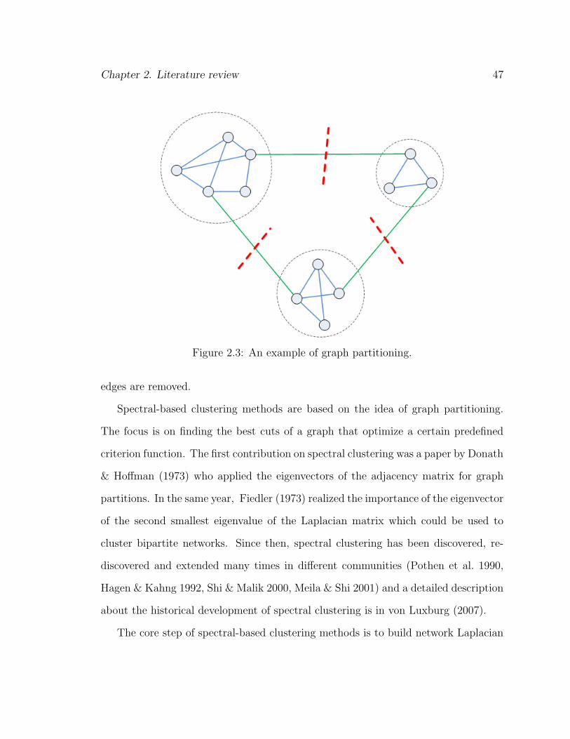
Chapter 2. Literature review 47
Figure 2.3: An example of graph partitioning.
edges are removed.
Spectral-based clustering methods are based on the idea of graph partitioning.
The focus is on finding the best cuts of a graph that optimize a certain predefined
criterion function. The first contribution on spectral clustering was a paper by Donath
& Hoffman (1973) who applied the eigenvectors of the adjacency matrix for graph
partitions. In the same year, Fiedler (1973) realized the importance of the eigenvector
of the second smallest eigenvalue of the Laplacian matrix which could be used to
cluster bipartite networks. Since then, spectral clustering has been discovered, re-
discovered and extended many times in different communities (Pothen et al. 1990,
Hagen & Kahng 1992, Shi & Malik 2000, Meila & Shi 2001) and a detailed description
about the historical development of spectral clustering is in von Luxburg (2007).
The core step of spectral-based clustering methods is to build network Laplacian
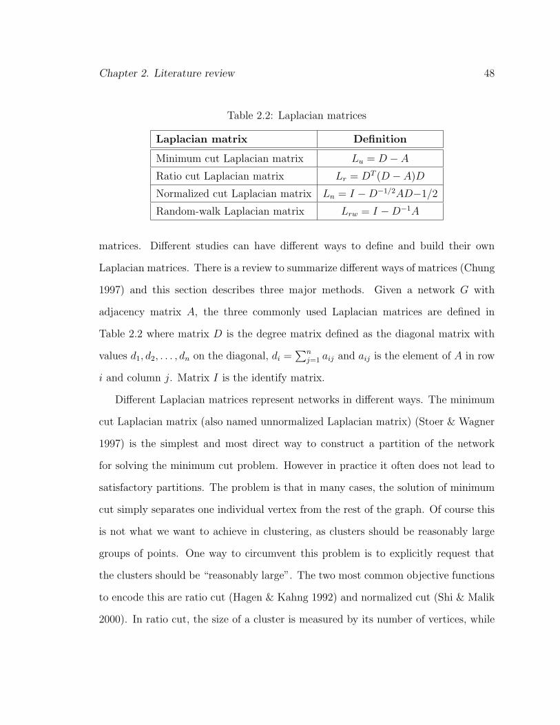
Chapter 2. Literature review 48
Table 2.2: Laplacian matrices
Laplacian matrix Definition
Minimum cut Laplacian matrix Lu = D − A
Ratio cut Laplacian matrix Lr = DT (D − A)D
Normalized cut Laplacian matrix Ln = I −D−1/2AD−1/2
Random-walk Laplacian matrix Lrw = I −D−1A
matrices. Different studies can have different ways to define and build their own
Laplacian matrices. There is a review to summarize different ways of matrices (Chung
1997) and this section describes three major methods. Given a network G with
adjacency matrix A, the three commonly used Laplacian matrices are defined in
Table 2.2 where matrix D is the degree matrix defined as the diagonal matrix with
values d1, d2, . . . , dn on the diagonal, di =∑n
j=1 aij and aij is the element of A in row
i and column j. Matrix I is the identify matrix.
Different Laplacian matrices represent networks in different ways. The minimum
cut Laplacian matrix (also named unnormalized Laplacian matrix) (Stoer & Wagner
1997) is the simplest and most direct way to construct a partition of the network
for solving the minimum cut problem. However in practice it often does not lead to
satisfactory partitions. The problem is that in many cases, the solution of minimum
cut simply separates one individual vertex from the rest of the graph. Of course this
is not what we want to achieve in clustering, as clusters should be reasonably large
groups of points. One way to circumvent this problem is to explicitly request that
the clusters should be “reasonably large”. The two most common objective functions
to encode this are ratio cut (Hagen & Kahng 1992) and normalized cut (Shi & Malik
2000). In ratio cut, the size of a cluster is measured by its number of vertices, while

Chapter 2. Literature review 49
in normalized cut the size is measured by the weights of its edges. The random walk
Laplacian matrix (Meila & Shi 2001) is based on random walks over the network.
The random walk Laplacian matrix can be interpreted as trying to find a partition
of the network such that the random walk stays for long within the same cluster and
seldomly jumps between clusters. It seems that there is no universal Laplacian matrix
and its definition can be tailored user requirements and similarity measures.
The success of spectral clustering is mainly based on the fact that it does not
make strong assumptions on the form of the clusters. As opposed to hierarchical
clustering where the resulting clusters form convex clusters, spectral clustering can
solve very general problems like intertwined spirals. Moreover, spectral clustering can
be implemented efficiently even for large data sets because the major calculation is
concentrated on a matrix calculation which is compatible with parallel computation
in distributed systems (Chen et al. 2011). This algorithm is not dependant on the
initialization and there are no issues of getting stuck in local minima or restarting
the algorithm for several times with different initializations.
Recently, spectral clustering-based studies have covered many areas in both ho-
mogeneous and heterogeneous networks. For homogeneous networks, Thurlow et al.
(2010) identified functionally related prognostic gene sets for head and neck squa-
mous cell carcinoma by applying spectral clustering on microarray data and found
gene sets highly significant for predicting patient outcome by grouping patients and
their genes into different clusters. Krzakala et al. (2013) compared spectral clustering
with different Laplacian matrices in some real world datasets and they found ran-
dom walk based spectral clustering outperformed others. Another study (van Gennip
et al. 2013) applied spectral clustering on a dataset combining social and geographical

Chapter 2. Literature review 50
data together and investigated the limitations of this method in the circumstance of
missing social data.
For heterogeneous networks, spectral clustering was firstly applied to bipartite
networks such as word-document data (Dhillon 2001, Ding et al. 2001). These algo-
rithms formulate the data matrix as a bipartite network and seek to find the opti-
mal normalized cut for networks. However, the clusters generated by these methods
contain vertices of both types. The following research aims at clustering different
types of objects into different clusters instead of mixing them. This type of spectral-
based clustering (called co-clustering or bi-clustering) is based on matrix factorization.
Studies (Dhillon et al. 2003, Long et al. 2005, Li 2005) model the co-clustering as an
optimization problem involving a triple matrix factorization. In their experiments,
they build a set of clusters for each type of object and recursively maximize the mu-
tual information between clusters with the same type of objects. A more generalized
co-clustering framework is presented by Zhong & Ghosh (2005) which can combine
with different optimization functions such as modularity and information entropy.
Later spectral-based clustering methods are extended to networks with more than
two types of data objects. Gao et al. (2005) formulated star-structured relational data
as star-structured multi-partite networks and this method allows users to define their
own optimization functions. Another important study was done by Long et al. (2006).
The study proposes a general model of clustering multi-type interrelated data object
simultaneously and the model is applicable to heterogeneous networks with various
structures. The method iteratively clusters each type of data objects and reinforces
the clustering quality of each type by the interactions among objects in different types
until convergence. This method also considers both object attributes and topological

Chapter 2. Literature review 51
features at the same time which extends its usage. However, there is no convergence
analysis, such as what kind of networks converge and how fast they will converge.
Till now, spectral-based clustering has become the major and most widely applied
community detection method for both homogenous and heterogeneous networks. A
drawback of recent spectral-based methods for heterogeneous networks which reduces
the efficiency is to cluster different types of objects simultaneously. The multiple
semantic-path clustering proposed in this thesis aims to cluster target object type
instead of all types of vertices. This improves the clustering efficiency significantly.
2.2.4 Modularity partitioning
Modularity partitioning is another class of community detection methods on net-
works. The concept of modularity is proposed by Newman (2004) and it was initially
introduced as a optimal function to define a stopping criterion for hierarchical clus-
tering. In other words, modularity is the goal of community detection. Of course
in different situations the definition of modularity can be different and modularity-
based clustering is an optimal function to maximize values of predefined modularity.
In the survey paper, Newman (2006) summarized and explained different definitions
of modularity and how they affect the clustering results.
The first algorithm developed for maximizing modularity is based on greedy al-
gorithms (Newman 2004). This algorithm is an agglomerative hierarchical clustering
method where vertices with high similarities are joined into small groups and then
small groups are connected to form large ones, thereby increasing the modularity.
The process of modularity maximization is this: it starts from |C| clusters where |V |is the number of vetices and each cluster has one vertex and edges are not added one

Chapter 2. Literature review 52
by one during the procedure. Adding the first edge to the set of disconnected vertices
reduces the number of groups from n to n− 1, so it generates a new partition of the
network. The edge is chosen such that this partition gives the maximum increase
of modularity with respect to the previous configuration. All other edges are added
based on the same principle. If the insertion of an edge does not change the partition,
i.e. the edge is internal to one of the clusters previously formed, modularity stays
the same. A later paper (Clauset et al. 2004) improves the efficiency of Newman’s
method. The previous approach involves a large number of useless operations due
to the sparse adjacency matrix and the revised method is more efficient when using
data structures for sparse matrices.
Although this approach to optimization of modularity tends to form large commu-
nities quickly, it often yields low values of maximum modularity. A study by Danon
et al. (2005) modifies the modularity to this: the merger of two communities depends
on the edge fraction of two communities so as to favor small ones. This trick leads to
a better modularity optima as compared to Newmans original approach.
Currently, modularity works mainly as an index to estimate the quality of clus-
tering in both homogeneous and heterogeneous networks instead of a community
detection method (Dhillon 2001, Dhillon et al. 2003, Long et al. 2005, 2006, Thurlow
et al. 2010, Meng & Kennedy 2012b, Wang et al. 2013). This thesis also applies New-
man’s modularity to evaluate the results of community detection in Chapter 3 and
Chapter 4.
Chapter 2. Literature review 53
2.2.5 Other community detection methods on heterogeneous
networks
As community detection on heterogeneous networks has become a topic of huge inter-
ests in network analysis, there are many new approaches developed for heterogeneous
networks.
The work starts from developing new similarity measures based on semantic paths.
Jeh & Widom (2002) proposed a similarity measure, SimRank, to calculate pairwise
similarity between objects in heterogeneous networks. This method is quite similar
to common neighbor similarity measures in homogenous networks and it counts path
numbers of each semantic path between two vertices. Although this similarity measure
treats the contribution of different semantic paths in the same way, it is still applied
by many studies (Jeh & Widom 2004, Fogaras & Racz 2005, Lin et al. 2006, Tian
et al. 2008, Li et al. 2010). A study by Lizorkin et al. (2010) combines SimRank with
optimization functions so as to improve the quality of clustering. He et al. (2010)
parallelize SimRank to improve its capability of processing large-scale datasets.
Another similarity measures, PathSim, is proposed by Sun et al. (2011). This
method involves a mechanism of semantic path selection through which this method
can choose semantic paths with high contributions. However, PathSim is not appli-
cable to asymmetric paths.
Sun & Han (2013) proposed a novel way to deal with the community detection
problem by combining clustering and ranking approaches. The method is based
on the idea that ranking and clustering can mutually enhance each other because
objects highly ranked in each cluster may contribute more towards an unambiguous
clustering. If an object is ranked high by one cluster, the object is more likely belong

Chapter 2. Literature review 54
to this cluster. Their experimental results demonstrate that the accuracy of clustering
results can be significantly enhanced. However, the scale of experimental data is too
small and covers the bibliography of only two areas (Data mining and database) in
the DBLP dataset.
Although there are many community detection methods proposed for heteroge-
neous networks, few of them consider that different users may have different purposes
for clustering. This thesis proposes a multiple semantic-path clustering in Chapter 3
which can select and estimate semantic paths with user guidance in order to achieve
user-desired clustering results.
2.2.6 Community detection validation
As reviewed in the previous sections, there are many algorithms to detect communi-
ties in networks and this requires a comprehensive set of ways to compare or evaluate
them. This section briefly reviews some state-of-the-art approaches for evaluating
community detection methods covering statistical indices, modularity and informa-
tion theoretic-based agreement measures. In this thesis, these approaches are applied
to assess the clustering results in Chapter 3 and Chapter 4.
In community detection, a community is roughly defined as “densely connected”
objects that are “loosely connected” to others. Whether a clustering is “good” or not
is determined by whether the detected communities follow this rule and how closely.
Many evaluation methods are proposed in accordance to this idea but with different
explanations of “internal density” and “external looseness”. For example, “density”
can either be the number of edges, the number of n-cliques or even the total number
of shared neighbors.

Chapter 2. Literature review 55
The most straightforward approach to validation is statistical analysis. The qual-
ity of clustering is evaluated by one or several indices. In this way, two independent
functions f and g are introduced, where f is used to measure the “density” inside the
clusters while g indicates the “looseness” among clusters. Till now, many different
indices are proposed based on different definitions of “internal density” and “external
looseness”. Among them, coverage and performance (Scott & Carrington 2011) are
two widely applied indices for evaluating the quality of community detection results.
This thesis applies them to evaluate the community detection results in Chapter 3
and Chapter 4.
1. Coverage is a common index in evaluating quality of clustering and the func-
tion f refers to the proportion of numbers of intra-cluster edges to all edges.
After clustering, every vertice must be allocated into clusters but edges may
exist among clusters. In order to achieve the purpose that edges are dense in
clusters and sparse among clusters, this proportion should be large. In weighted
graphs, this proportion represents the ratio of the sum of edge weights in clus-
ters to the sum of all edge weights. In unweighted graphs, it is the number of
edges. The function g is always zero in this approach.
2. Performance first defines a “correct” and “incorrect” clustering which refers
to the connectivity of vertices. If two vertices are in the same cluster and there
is an edge between them or they are in different clusters and there is no edge
between them, they are labeled as a “correct” clustering. Otherwise, they are
“incorrect”. Based on this, function f is defined as counting the number of
edges in clusters whereas g counts the number of nonexistent edges between
clusters.

Chapter 2. Literature review 56
However, the values of these indices are influenced by the number and the size of
communities. A slight difference in the number of communities and sizes may give rise
to a huge differences in indice values. For example, a good division of a network into
communities is not merely one in which there are few edges between communities;
it is one in which there are fewer than expected edges between communities. If
the number of edges between two groups is significantly less than expected, this
means that the division is effective as it shows meaningful community structure. This
idea, that the true community structure in a network corresponds to a statistically
surprising arrangement of edges, can be quantified by using the measure known as
modularity (Newman & Girvan 2004) which is roughly the number of edges within
communities minus the expected number in an equivalent network with edges placed
at random. Indeed, modularity has multiple usages: it was initially proposed to
be a clustering method (Clauset et al. 2004); later it also served as an optimization
approach to improve clustering results by other methods (Newman 2006); and recently
it is often adopted as a evaluation of clustering quality (Shen et al. 2009).
The approach for calculating modularity follows Newman’s formula which was
proposed to work on unweighted networks. Consider a network G = (V,E), the
modularity of this network is
Q =1
4|E|CTBC (2.2.3)
where matrix C is a cluster indicator matrix of the network and Ci,j = 1 denotes that
the ith vertex belongs to the jth community. Matrix B is the modularity matrix and
it is defined as
Buv = Auv − dudv2|E| (2.2.4)
where A is the association matrix and du and dv are the degrees of vertex u and v

Chapter 2. Literature review 57
respectively.
The modularity can be either positive or negative, with positive values indicating
the possible presence of community structure. Thus, one can search for community
structure precisely by looking for the divisions of a network that have positive and
preferably large, values of the modularity.
Another way to evaluate clusters involved in this thesis is the information theoretic
agreement measure, Normalized Mutual Information (NMI) (Batina et al. 2011) which
computes the agreement between two given partitions or between a partition and the
ground truth. This evaluation is applied in Chapter 3 for verifying how to acquire a
desired clustering.
Given a network with n vertices, there are two partitions X and Y with x and y
clusters respectively. For partition X, the clusters are labeled as 1, 2, . . . , x while for
partition Y the clusters are labeled as 1, 2, . . . , y. In NMI, partitions are regarded as
the different distributions of vertices. As a result, the normalized mutual information
Inorm(X, Y ) is defined as
Inorm(X, Y ) =2I(X, Y )
H(X) +H(Y )(2.2.5)
I(X, Y ) =x∑
i=1
y∑j=1
PXY (i, j) logPX(i, j)
PY (i)P (j)
H(X) = −x∑
i=1
PX(i) logPY (i)
H(Y ) = −y∑
j=1
PY (j) logPY (j)
where PX(i) stands for the probability of objects belonging to Cluster i in partition X
and PY (j) stands for the probability of objects belonging to cluster j in partition Y .

Chapter 2. Literature review 58
PXY (i, j) is a joint probability, denoting the probability of objects belonging to both
cluster i in partition X and cluster j in partition Y . The measure I(X, Y ) tells how
similar partition X and Y are. The value of NMI is zero when two distributions are
independent and one when they are identical.
Normalized Mutual Information, which is derived from probability theory and in-
formation theory, is a reliable method for measuring the mutual dependence of two
random variables (Paninski 2003). It is applied in many papers (Lancichinetti et al.
2008, Lancichinetti & Fortunato 2009, Blondel et al. 2008) for comparing clustering
quality among different community detection algorithms because of its sound theo-
retical basis and easy implementation.
2.3 Determining the number of clusters
In networks, choosing the number of clusters k in advance is a general problem for
nearly all clustering algorithms and the choice of “right” number of clusters can
improve the quality of clustering substantially because the number of clusters is a
mandatory input parameter of many state-of-the-art and widely applied clustering
methods such as K-means and spectral clustering. There are two main families of
approaches: clustering result-based methods and topological feature-based methods.
2.3.1 Clustering result-based methods
In a real dataset, the number of clusters is often unknown. The simplest method
of choosing the number of clusters is to try different values, and cluster valida-
tion techniques are used to measure the clustering results and determine the best

Chapter 2. Literature review 59
value of k (Calinski & Harabasz 1974, Hartigan 1975). These approaches where
the clustering algorithms are repeatedly executed are computationally expensive and
time-consuming. To extend the availability of this idea, Kryszczuk & Hurley (2010)
integrate the process of multiple execution of clustering algorithms and clustering
comparison into a standard, general framework where the framework is compatible
with different clustering validity indices (Maulik & Bandyopadhyay 2002) including
modularity, performance and coverage. These are a group of functions measuring
the clustering quality. Although this proposed method is very effective in finding the
correct number of clusters in benchmark datasets, it is still confined to small datasets.
2.3.2 Topological feature-based methods
Recently with the emergence and rapid expansion of social, biological and biblio-
graphic networks, the problem of determining the number of clusters becomes more
challenging because the traditional approach to repeatedly execute the clustering al-
gorithms is impractical with these large-scale datasets. Then the problem has been re-
considered from the aspect of the clustering algorithms based on topological features.
As presented in the previous section, topological features and community structures of
networks can be understood to some extent through the analysis of their correspond-
ing matrices such as adjacency or Laplacian matrices. From this idea, the number of
clusters is determined by how many eigenvalues are chosen and therefore the methods
in this area are usually based on the eigenvalue structure (Fraley & Raftery 2002).
Cumulative percentage variance (Abdi &Williams 2010) is an accurate method
for determining the number of clusters based on matrices built from networks. As
different eigenvalues contribute differently to the network partition, an intuitive idea

Chapter 2. Literature review 60
Figure 2.4: Scree graph
is to choose those important eigenvalues. In spectral-based clustering, smaller eigen-
values are more important than larger ones in terms of network partitioning. Assume
that there are m eigenvalues and the first k smallest eigenvalues are chosen. The
cumulative percentage variance is defined as
C = 1−∑k
i=1 li∑mj=1 lj
(2.3.1)
where li is the ith smallest eigenvalue of the Laplacian matrix. However, this method
does not solve the problem completely but transfers it to a new question on how to
choose C.
Another better way to choose k is with a scree graph (Jolliffe 2005). A scree
graph, shown in Figure 2.4, is a plot of eigenvalues associated with vertex indices. In
general, the “elbow point” is the separation and the eigenvalues which are less than
it are chosen. For example, in Figure 2.4, eigenvalues with index 2 should be chosen.
One way to find the “elbow point” is to compare the slope between both sides of

Chapter 2. Literature review 61
eigenvalues with the “elbow point” having the maximum value. The slope value is
defined as
S(k) = (lk−1 − lk)− (lk − lk+1) (2.3.2)
where lk is the kth smallest eigenvalue of the Laplacian matrix.
There are many similar methods and examples include ad hoc measures such as
the ratio of within-cluster and between-cluster similarities (Chiang & Mirkin 2010),
information-theoretic criteria (Still & Bialek 2004), the gap statistic (Tibshirani et al.
2001) and stability approaches (Lange et al. 2004).
Although many methods are proposed, it is still hard to give a general answer
to the question of how many eigenvalues to choose as different methods have their
own advantages in different types of networks. For example, the methods based on
the ratio of within-cluster to between-cluster similarities perform better on networks
with a clear community structure. Lange et al. (2004) comprehensively describes the
above methods and explains the different usages of them. The study applies K-means
on 20 randomly generated datasets with different numbers of clusters determined
by different approaches. The performances of the different methods vary when the
generated networks show different topological features like density.
Indeed, choosing which approach is suitable for determining the number of clusters
requires a deep understanding of networks and indeed this information is hard to
retrieve before clustering. However the current researches confirm that determining
the number of clusters from topological features is feasible.
This thesis is inspired to continue to address the problem by considering network
topology and finds that social network theory proposes a completely new idea. In
social science, the reason why social networks tend to have a community structure

Chapter 2. Literature review 62
is because different individuals play different roles and roles are reflected through
their topological features (Scott & Carrington 2011). More specifically, some objects
are considered to be more important in terms of topological features than others as
they are the core of groups and the regular members are linked to each other via
them. Those objects with high ranks in significance are defined as “group leaders”
and the number of clusters is highly related to the number of those leaders. The
early research (Sparrowe et al. 2001, Mehra et al. 2006) attempted to detect leaders
via degree centrality as they believed that leaders should have more links with oth-
ers. However, they ignored an important fact that in the real world, core members
sometimes have a high degree-centrality (Abbasi et al. 2011) as well. As a result, the
number of detected leaders is often more than the real number of leaders.
This thesis (Chapter 4), therefore, involves betweenness-centrality (Baglioni et al.
2012) to remedy the methods for searching for leaders because leaders not only have
more connections in clusters but they also often relate with individuals in other clus-
ters and betweenness centrality, that quantifies the number of times a vertex acts as a
bridge along the shortest path between two other vertices, can reflect this character-
istic. Meanwhile, considering the case that sometimes there are two or more leaders
in one potential group, this thesis devises an algorithm to combine leaders when they
are close enough. Beside “group leaders”, this thesis defines “group coordinators”
who mainly take responsibility to connect groups together. For example, in academic
collaboration network, directors of research centers are the coordinators of research
labs. Removing the edges between “group coordinators” in advance may make the
work of community detection much easier. Finally a novel community detection ap-
proach based on the concept of “roles” is proposed. Because leaders are detected

Chapter 2. Literature review 63
Figure 2.5: SVM aims to draw a boundary among objects and those objects in thesame side are classified into one cluster (Cortes & Vapnik 1995).
by Support Vector Machine (SVM) based on training datasets, next section briefly
reviews SVM methods.
2.3.3 Support Vector Machine (SVM)
Support Vector Machine (SVM) is a kind of binary classification method (Moya &
Hush 1996). This classification method tries to identify objects belonging to two
classes amongst all objects, by learning from a training set containing positive and
negative examples of objects. According to the problem of determining the number
of clusters, this thesis applies SVM to find leaders from all objects.
In binary classification methods, Support Vector Machine (Cortes & Vapnik 1995)
of them outperform others in terms of generalization. This method was initially
proposed in 1995 but the concept could be traced back to 1979 (Cortes & Vapnik
1995).
Chapter 2. Literature review 64
Support Vector Machine aims to find the optimal boundaries between two groups
of objects and these optimal boundaries are decided by involving different kernel func-
tions. Unlike traditional methods which minimize the empirical training error, Sup-
port Vector Machine minimizes an upper bound of the generalization error through
maximizing the margin between the separating hyperplane and the data. Another at-
tractive aspect is that it can be compatible with different kinds of kernel functions (a
distance measure between objects). Therefore it can be linear or non-linear.
In the thesis, Support Vector Machine with Gaussian kernel function is applied to
find leaders in a heterogeneous co-authorship network and the followed procedure of
non-linear SVM refers to Burges (1998).
2.4 Link prediction
The link-prediction problem for social networks can be described from the point of
view of data mining in the following way: given a snapshot of a social network at
time t, the goal is to predict new links that will be added to the network during the
interval from time t to a given future time t′.
This problem can be viewed as a simple binary classification problem. That is,
for any two potentially linked objects oi and oj, predict whether lij is 1 or 0. Current
research aims to measure the degree of similarity and closeness between two target
nodes. In network terms this means not only that they should be similar to each other,
but also that they must also be reachable through the network. In other words, the
closer and more similar are they, the higher possibility they have to be connected in
the future. Generally, approaches to address this problem come from two aspects:
the attribute information of nodes and the structural properties of social networks.

Chapter 2. Literature review 65
In the first of these kinds of approach, attribute information is used for link
prediction. Popescul & Ungar (2003) introduces a structured logistic regression model
that can make use of relational features to predict the existence of links on citation
datasets from CiteSeer. In that experiment, link prediction on citation networks is
cast into a citation recommendation system by gauging similarities between target
publications and existing publications. However, those methods have limitations in
that the attributes of nodes can only reveal similarity with others, but fail to take
the concept of “distance” into consideration. For instance, two people may be quite
similar to each other in terms of habits, interests and backgrounds. However, they
cannot be friends if they are located far from each other in geography as they have
no chance to meet.
Links are predicted on the basis of different graph proximity measures. Among the
selection of proximity measures, nearest neighbourhood algorithms are quite famous
and have been widely applied. In the experiment of Murata & Moriyasu (2008),
they introduced a weighted common neighbour approach and compared its prediction
results with common neighbour and Jaccard’s coefficient method. Unfortunately,
their experimental results have accuracies that are all lower than 50%.
The reason for this is because neighbourhood algorithms can make correct predic-
tion when two nodes are quite close to each other. In fact, some relationships such
as friendship, co-authorship and citation relationships are transitive: nodes may be
connected in the future if there is a path among them, but those methods may ignore
this situation.
The second approach takes into account the structural properties of social net-
works, namely “distance” between nodes, when devising measures of closeness. One

Chapter 2. Literature review 66
famous approach is the Katz measure (Katz et al. 1997) which defines a measure that
directly sums over the collection of paths, exponentially damped by their length so
as to count short paths more heavily. Another approach uses random walk (Rud-
nick & Gaspari 2004), to calculate the moving time or number of steps of an agent
from a start point s to the end point e. Because the time to arrive is not in general
symmetric, a common way to detect closeness from this probabilistic approach is to
consider the commute time Cs,e = Ts,e + Te,s, where Ts,e and Te,s are times to move
from start to end and end to start respectively. Liben-Nowell & Kleinberg (2007)
present an experiment comparing predictors on large co-authorship networks. Their
work suggests that information about future interactions can be extracted from the
network topology alone and that subtle measures for detecting node proximity can
outperform more direct measures. However, the results show that among all predic-
tors, Katz, the method combining neighbourhood and distance concepts, is the best.
However, the accuracy they found of 16% is still quite low.
The above research confirms that current methods of link prediction have a large
room for improvement. In this thesis, information concerning the evolution of a co-
authorship network is collected so as to treat vertices differently. Through observing
their past actions, vertices are labeled by their activities and those vertices with
high values in activity have a high possibility to connect with others. In order to
improve the accuracy further, matrix theory is applied to detect the main patterns
of predicting results.

Chapter 2. Literature review 67
2.5 Ranking
Early stages of ranking objects in networks focused on object connectivity. The
initial research on ranking vertices in networks is inspired by the voting mechanism
that highly ranked objects are those who get more votes from others. Based on this
idea, highly ranked vertices in networks should have more connections from others.
For this reason, Brin & Page (1998) proposed the famous PageRank algorithm to rank
web pages based on keywords that user input and webpage connectivity. Till now this
idea is still the core algorithm of Google search engine. Since then, many studies have
been devoted to this area and have proposed many customized PageRank algorithms
(a comprehensive review about PageRank algorithms and their applications can be
found in Berkhin (2005)).
Kleinberg (1999) first extended the ranking work from homogeneous networks
to heterogeneous networks. His famous method, the Hyperlink Induced Topic Search
(HITS), confirms that ranking can be reinforced through interactions between nodes of
various types. As a result, many famous papers with a few citations can be assigned
high ranks. Since then, numerous papers on link analysis–based ranking based on
PageRank or HITS have appeared (Ahmedi 2012, Fiala 2012).
Recent advances in graph theory and corresponding methods have enriched rank-
ing methods by incorporating topological features. It is believed that in networks,
an object is ranked high, if it is located in an important position. Many centrali-
ties (Scott 2012) are proposed to achieve this purpose. Liu et al. (2005) compared
the rankings of scientists by PageRank with three other rankings using degree, be-
tweenness centrality and closeness centrality. The results confirmed that centrality

Chapter 2. Literature review 68
measures are effective each with their own advantages and that without consider-
ing citations, famous but not so highly cited papers are ranked very high. Another
work (Chiang et al. 2012) exploits social links and uses local information only to
find the top-k users in a co-authorship network based on a probabilistic model using
random walks.
Soon, the research focus of ranking moves to heterogeneous networks. Deng et al.
(2012) proposed a joint regularization framework to model heterogeneous networks
and treated multi-typed linking edges differently, which is effective to ranking objects
in heterogeneous networks. Sun & Han (2012) proposed a new ranking approach
called Authority Ranking for heterogeneous networks. The main idea is that the
rank of an object in a heterogeneous network is determined by its authority and that
authors can be clustered by authority. For example, highly ranked authors tend to
attend highly ranked venues and highly ranked venues attract highly ranked authors.
The approach is applied to co-ranking authors and venues on the DBLP dataset and
the experimental results are very effective. However, this method can only work for
bipartite networks.
Inspired by the previous work, this thesis develops a co-ranking method based
on both object connectivity and topological features for heterogeneous network. The
proposed method can rank objects in complex heterogeneous networks where one-
type of objects can connect to other types of objects or themselves. For testing
the effectiveness and efficiency, two state-of-the-art ranking methods, PageRank and
Hyperlink-Induced Topic Search (HITS), are involved for comparison.

Chapter 2. Literature review 69
2.6 Research gaps
In summary, this chapter reviews current research on four basic network analysis
questions: detecting communities, determining the number of clusters, predicting
links and ranking vertices in both homogenous and heterogeneous networks. The
major identified research gaps are listed below.
The complex topological features of heterogeneous networks give rise to one major
issue in community detection: how to estimate the contributions of different relation-
ships, especially for abstract concepts. The current community detection methods on
heterogeneous networks (reviewed in Section 2.2) fail to provide an applicable way for
users to estimate contributions to relationships and ignore that different users may
have different purposes for clustering. This thesis proposes a multiple semantic-path
clustering method which can achieve a desired clustering with user-guided informa-
tion.
The major way of determining the number of clusters is via eigenvalue structures
of networks. Different eigenvalues are of different importance for having network
topological information. In spectral-based clustering algorithms, smaller ones are
more important than larger ones. However, the number of leading smallest eigenvalues
to choose is hard to determine. This thesis addresses the problem by considering
network topology. The proposed method in Chapter 4 determines the number of
clusters by finding cores of communities which are labeled as leader groups.
For link prediction, the major issue is that the link prediction accuracy is still
low and there is a large room to improve. The current methods predict links via
vertex similarities. If two vertices are similar, they are likely to connect; otherwise,
they have a small possibility to connect in the future. In fact, there are often some

Chapter 2. Literature review 70
exceptions that dissimilar vertices are connected while similar ones are not connected
and this is the major reason why link prediction accuracy is low. This thesis proposes
a network evolution-based link prediction method which can capture these exceptions
based on vertex evolving patterns.
For vertex ranking, the current studies of ranking vertices in heterogeneous net-
works focus on bipartite networks where there are two types of vertices and one type
of vertex is not connected directly but connect to each other indirectly via the other
type of vertex. The proposed co-ranking method in Chapter 6 can work on complex
bipartite networks where one type of vertex can connect directly or indirectly.

Chapter 3
Community detection onheterogeneous networks
In the real world, there are many abstract social phenomena like academic collab-
oration which are hard to measure directly. An approach to solving this problem
is to decompose abstract concepts into a set of concrete and measurable ones. For
example, academic collaboration can be represented by co-authorship and co-work
relationship. This practice gives rise to heterogeneous networks.
Compared with homogeneous networks, heterogeneous networks always contain
different types of objects which are connected by different types of relations. Because
of this topological complexity, many traditional ways of community detection de-
signed for homogeneous networks are not feasible. To solve this problem, this chapter
proposes a Multiple Semantic-path Clustering method which is a general approach of
community detection on heterogeneous networks based on paths and matrix factor-
ization (Tang & Liu 2010). This method can also achieve a desired clustering based
on user-guided information.
71
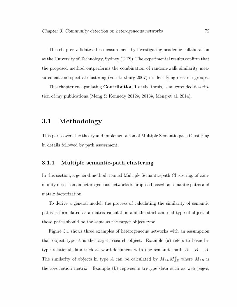
Chapter 3. Community detection on heterogeneous networks 72
This chapter validates this measurement by investigating academic collaboration
at the University of Technology, Sydney (UTS). The experimental results confirm that
the proposed method outperforms the combination of random-walk similarity mea-
surement and spectral clustering (von Luxburg 2007) in identifying research groups.
This chapter encapsulating Contribution 1 of the thesis, is an extended descrip-
tion of my publications (Meng & Kennedy 2012b, 2013b, Meng et al. 2014).
3.1 Methodology
This part covers the theory and implementation of Multiple Semantic-path Clustering
in details followed by path assessment.
3.1.1 Multiple semantic-path clustering
In this section, a general method, named Multiple Semantic-path Clustering, of com-
munity detection on heterogeneous networks is proposed based on semantic paths and
matrix factorization.
To derive a general model, the process of calculating the similarity of semantic
paths is formulated as a matrix calculation and the start and end type of object of
those paths should be the same as the target object type.
Figure 3.1 shows three examples of heterogeneous networks with an assumption
that object type A is the target research object. Example (a) refers to basic bi-
type relational data such as word-document with one semantic path A − B − A.
The similarity of objects in type A can be calculated by MABMTAB where MAB is
the association matrix. Example (b) represents tri-type data such as web pages,

Chapter 3. Community detection on heterogeneous networks 73
Figure 3.1: Examples of semantic paths.
web users and search queries in web search engines with two paths A − C − A and
A−C−D−C−A. There are two association matrices MAC and MCD and therefore
the similarity of objects in type A can be represented by the combined similarity
of two paths. The similarities of these paths can be calculated by MACMTAC and
MACMCDMTCDM
TAC respectively. Example (c) is a much more complex homogeneous
networks with five object types and objects A are linked both directly and indirectly.
The possible paths are A−A, A−C −A, A−C −B −C −A, A−C −D−C −A
and A−C−E−C−A. In this case, the similarity of A-type objects is the collective
similarities of all these paths.
Definition 3.1. Given a heterogeneous network G = (V,E), there are m different
types of object (V1, . . . , Vm) and n types of relation (E1, . . . , En). Each type of object
may contain different number of vertices. If the target object type is Vt with |Vt|vertices (1 ≤ t ≤ m). The corresponding semantic path set of this target object type

Chapter 3. Community detection on heterogeneous networks 74
is Pt, the collective similarity of objects in type Vt is defined as
SVt =
|Pt|∑i=1
aiSi s.t.
|Pt|∑i=1
ai = 1 (3.1.1)
where SVt is the collective similarity matrix of target objects Vt while matrix Si is the
similarity matrix of target objects Vt in terms of path i. There is scale parameter ai
which indicates the contribution of semantic path i to the collective similarity SVt .
It has been shown that the hidden structure of a data matrix can be explored
by matrix factorization (Tang & Liu 2010). Motivated by this finding, the clustering
process of multiple semantic-path clustering is based on matrix factorization because
the cluster structure for a type of objects Vt is embedded in the collective similarity
matrix SVt and the cluster structure of Vt is revealed by the triple factorization,
RVt ≈ CVtSVtCTVt
= CVt
⎛⎝ |Pt|∑
i=1
aiSi
⎞⎠CT
Vt(3.1.2)
where CVt ∈ {0, 1}|Vt|×k is a cluster indicator matrix for target object Vt and k is
the number of clusters such that CVt(p, q) = 1 denotes that the pth object in Vt is
associated with the qth cluster and∑k
q=1 CVt(p, q) = 1.
Based on the above discussions, the task of Multiple Semantic-path Clustering on
heterogeneous networks can be formally defined as the following optimization problem
and the optimization function below is the objective function of the proposed Multiple
Semantic-path Clustering method.
minF (CVt) =
⎛⎝RVt − CVt
⎛⎝ |Pt|∑
i=1
aiSi
⎞⎠CT
Vt
⎞⎠ (3.1.3)
The minimization in Equation (3.1.3) is equivalent to the maximization in Equa-
tion (3.1.4). An iterative algorithm is proposed to determine the optimal solution to

Chapter 3. Community detection on heterogeneous networks 75
the maximization problem.
maxG(CVt) =
⎛⎝CVt
⎛⎝ |Pt|∑
i=1
aiSi
⎞⎠CT
Vt
⎞⎠ (3.1.4)
Although the maximization problem in Equation (3.1.4) is NP-hard, the solution
of which cannot be found in polynomial time, an approximate solution can be achieved
by a relaxation by converting the cluster indicators from discrete ones to continuous
values using spectral graph partitioning (Ding et al. 2010).
Multiple Semantic-path Clustering clusters multi-type interrelated data objects
based on their relations by exploiting both direct and indirect interactions between
the hidden structures of different types of objects via semantic paths and matrix fac-
torization. The proposed Multiple Semantic-path Clustering method is an extension
of traditional spectral graph partitioning for community detection. As a result, it
inherits many advantages such as achieving a global solution, having a theoretical
support and easy implementation.
3.1.2 Semantic path assessment
In the previous section, all paths in multiple semantic-path clustering have scalars
that denote their relative importance when clustering target objects. However, het-
erogeneous networks, especially complex ones, always have a large set of semantic
paths. Consequently, the corresponding similarity calculations will be time and labor
intensive. It is necessary to know which semantic paths are important and the value
of their weights before clustering. This section explains how to choose scalars for
different semantic paths.

Chapter 3. Community detection on heterogeneous networks 76
In fact, semantic paths can be considered as features and path assessment is a pro-
cess of feature selection and estimation. Given a heterogonous network with p seman-
tic paths, there is a training dataset where users label the objects with cluster indic-
tors. The correlations between semantic paths and cluster indictors are b1, b2, . . . , bl
from largest to smallest. If the first l (l ≤ p) paths are chosen, the weights of paths
are defined as
ai =bi∑li=1 bi
s.t.
l∑i=1
ai = 1 (3.1.5)
In the experiment, academic collaboration at University of Technology, Sydney is
considered as a ground truth. Based on this, a sample is formed where researchers are
labeled with their laboratories. The weight of a path is represented by the correlation
between the path and cluster labels and paths with the leading closest correlations
are chosen as the main features.
3.2 Clustering evaluation
The proposed multiple semantic-path clustering method to detect communities on
heterogeneous networks is validated from the following two aspects: cluster compar-
ison and cluster validation.
3.2.1 Cluster comparison
To verify the effectiveness and efficiency of multi-path clustering, a well known com-
munity detection method, spectral clustering (a comprehensive description about this
method can be found in literature review, Section 2.2.3.) is involved for comparison.
However, spectral clustering cannot be applied on heterogeneous networks directly.
Chapter 3. Community detection on heterogeneous networks 77
To overcome this, a random-walk similarity measure is applied to build a similarity
matrix which spectral clustering can work on. In the experiment, as the current
laboratory setting of UTS is regarded as a ground truth, the clustering results gen-
erated by multi-path clustering and spectral clustering are compared with the UTS
laboratory settings.
The first approach for cluster comparison refers to vector comparison. It is appar-
ent that clustering results can be represented by an indicator matrix and the element
of the matrix indicates whether two data points are in the same cluster or not. Given
two partitions X and Y with n data points, there are two matrices MX and MY
built from these two partitions respectively. For partition X, if object i and j are
in the same clusters, MX(i, j) = 1; otherwise MX(i, j) = 0. The similarity between
partition X and Y is well defined as
Similarity(X, Y ) =1
n
n∑i=1
Vi · Ui
||Vi|| · ||Ui||Vi ∈ MX s.t. MX = (V1, . . . , Vn) (3.2.1)
Ui ∈ MY s.t. MY = (U1, . . . , Un)
where Vi and Ui are the vectors belonging to matrices MX and MY respectively.
Another comparison approach is Normalized Mutual Information (NMI) 2.2.6
which computes the agreement between two given partitions or between a partition
and the ground truth. This chapter regards the UTS laboratory settings as a ground
truth and it compares the clustering results by the proposed method and spectral
clustering with the ground truth.

Chapter 3. Community detection on heterogeneous networks 78
Figure 3.2: The constitution of Field of Research (FoR) codes
3.2.2 Cluster validation
Besides that, the clusters generated by multi-path clustering and spectral clustering
are also verified and compared by a set of clustering validation methods including
Coverage, Performance (Scott & Carrington 2011) and Modularity (Newman 2006).
The detailed descriptions about them are included in literature review (Section 2.2.6).
3.3 Experimental dataset
The dataset used for analysis and visualization is from the University of Technology,
Sydney (UTS) research master enterprise (RME) database, which is a collection of
over 60000 records, covering all the faculties and schools in UTS. Information on all
publications of UTS during the recent six years (2006− 2011) was selected including
journals, conference papers and proceedings, chapters and books of all faculties.
The distinctive advantage of this data source over other scientific bibliographic
databases like CiteSeer and computer sciences bibliographic data source DBLP is its
integrity. Although the number of records from this data source is relatively small

Chapter 3. Community detection on heterogeneous networks 79
compared to those scientific bibliographic databases, it contains more types of publi-
cations, research fields and researchers. Due to its integrity, it is easier to understand
academic collaboration in this closed environment. The data for verification such as
the configuration of laboratory settings and research leaders is easily accessed.
Besides researchers, faculties, roles and papers, another important object is intro-
duced to build the academic collaboration and it is Field of Research (FoR) codes.
They are used by Australia and New Zealand to indicate which research field publica-
tions belong to. Field of Research (FoR) codes are a system with 6 digits containing
three hierarchical levels: divisions (first 2 digits), groups (first 4 digits) and fields (all
6 digits) with divisions at the highest level. For example, the FoR code for Pattern
Recognition and Data Mining is 080109 while 08 is for Information and Computing
Sciences and 0801 stands for Artificial Intelligence and Image Processing. How one
publication belongs to different research fields is represented by percentages with each
publication having at most three FoR codes. For example, the journal article “Genetic
algorithm-based strategy for identifying association rules without specifying actual
minimum support” (Yan et al. 2009) is attached to three FoR codes: 080100 Artifi-
cial Intelligence and Image Processing (50%), 080604 Database Management (30%)
and 010200 Applied Mathematics (20%).
After data cleaning, integration, transformation and reduction (Han & Kamber
2006), the number of remaining records are stored in nine files: researcher file, pub-
lication file, FoR code file, faculty file, role file, researcher-publication relationship
file, publication-FoR codes relationship file, researcher-faculty relationship file and
researcher-role relationship file (See Table 3.1). Researchers file, publication file, FoR

Chapter 3. Community detection on heterogeneous networks 80
Figure 3.3: The schema of the network presenting the academic collaboration at UTS
codes file, faculty file and role file contain five types of nodes: researchers, publica-
tions, FoR codes, faculties and roles respectively, while the relationship files are used
to add links among the nodes.
Table 3.1: The number of records in files from 2009 to 2011
File name Number of records
Researcher file 5621
Publication file 3737
FoR code file 585
Faculty file 13
Role file 5
Researcher-Publication relationship file 12105
Publication-FoR codes relationship file 4576
Researcher-Faculty relationship file 5621
Researcher-Role relationship file 5621
The schema of the heterogeneous UTS academic collaboration networks is illus-
trated in Figure 3.3. It shows that researchers (R) are the core research objects.
Researchers are not linked to each other directly but through other objects (Facul-
ties (F ), Roles (L), Papers (P ) and FoR codes (C)). To be specific, researchers (R)

Chapter 3. Community detection on heterogeneous networks 81
can have different roles (L) such as professors, associate professors, senior lecturers,
lecturers and research followers. Different researchers (R) may belong to different fac-
ulties (F ) while researchers (R) publish papers (P ) which belong to FoR codes (C).
Finally, the information about the research organizational structure of UTS is
collected as the ground truth of academic collaboration. This information includes
researchers (R), laboratories (B) and working relationships (R− B −R).
3.4 Experimental results
This section evaluates the performance of the proposed multiple semantic-path clus-
tering on achieving a user desired community detection covering collective similarity
calculation, path assessment and cluster validation. The proposed method is applied
on the heterogeneous UTS academic collaboration network which involves multi-typed
objects and relationships to represent an abstract concept: academic collaboration.
Multiple semantic-path clustering can integrate different types of relationships by
assigning scalars to these relationships with user-guided information.
3.4.1 Collective similarity calculation
This section investigates the schema of the heterogeneous networks from UTS, de-
scribes the process of collective similarity calculation and explains that different
weights of semantic paths influence the collective similarities among researchers sig-
nificantly.
The experimental object is the UTS academic collaboration network. According
to the collected dataset in Section 3.3, it is a heterogeneous network with five object

Chapter 3. Community detection on heterogeneous networks 82
Figure 3.4: Semantic paths derived from the academic collaboration heterogeneousnetworks.
types (Researchers (R), Faculties (F ), Roles (L), Papers (P ) and FoR codes (C)) and
the 4 types of relation. In this experiment, researchers (R) are the target objects and
Figure 3.4 illustrates all semantic paths related to researchers (R).
Table 3.2: Similarity calculation of all semantic paths related to researchers.
Path Similarity calculation
R− F −R MRFMTRF
R− P − C − P −R MRPMPCMTPCM
TRP
R− P −R MRPMTRP
R− L−R MRLMTRL
The similarity of researchers (R) in each path can be calculated through matrix
computation. Given a path R− P −C − P −R where R is the set of target objects,
the similarity of R in the path is marked as MRPMPCMTPCM
TRP where MRP and
MPC are the adjacency matrices between object types R and P and between object
types P and C respectively. MTRP is the transposed matrix of MRP and MT
PC is
the transposed matrix of MPC . The collective similarities between researchers are

Chapter 3. Community detection on heterogeneous networks 83
measured by the similarities of those paths. The ways of calculating similarities of
each path is presented in Table 3.2 and the collective similarities of researchers (R)
are the combinations of these similarities.
3.4.2 Path assessment
If different weights are assigned to the paths, collective similarities of researchers (R)
may be fairly different. That is why different types of objects and relations must be
involved so as to reflect real situations in this domain.
Table 3.3: The paths and their corresponding scalars
Path Scenario I Scenario II Scenario III
R− F −R 0.97 0.01 0.05
R− P − C − P −R 0.01 0.01 0.28
R− P −R 0.01 0.97 0.62
R− L−R 0.01 0.01 0.05
To clarify this point further, this chapter designs three scenarios (Table 3.3) and
these scenarios have different scalar combinations. To be specific, Scenario I and
Scenario II overly emphasizes paths R− F −R and R− P −R respectively but put
very small weights (0.01) on the other paths. By contrast, the weight combination
in Scenario III are based on Pearson correlations (Kantardzic 2011). The weights
of each path are determined by this way (refer to Section 3.1.2): a random sample
dataset is built with 200 researchers and they are labeled with their laboratories; then
the similarities of each path are normalized and the weights of paths are represented
by the correlation between each path and the laboratory labels.
In this chapter, researcher similarity networks are built based on each of these

Chapter 3. Community detection on heterogeneous networks 84
Figure 3.5: The similarity graph of researchers in Scenario I
scenarios.
In Scenario I, faculties (F ) and the “belonging to” relation between researchers (R)
and faculties (F ) are emphasized to a large extent. The weight of this path is 0.97
while the remaining three paths are 0.01 respectively. The similarity graph of re-
searchers (R) is illustrated in Figure 3.5 which shows that researchers (R) are grouped
by the faculties.

Chapter 3. Community detection on heterogeneous networks 85
Figure 3.6: The similarity graph of researchers in Scenario II
Scenario II lays emphasis on co-authorship (0.97). This relationship connects two
authors together if they coauthored papers and the more papers they worked on, the
larger the weight of the connection. Co-authorship is also a widely used relation in
terms of academic collaboration research. However the detected groups (Figure 3.6)
are relatively small and meaningless because each author’s number of papers is lim-
ited, normally ranging from three to five. Thus it is necessary to consider other types
of objects and relations such as faculties (F ) and field of research codes (C).
Similarly if the other two paths are overemphasized, it is also difficult to under-
stand the real academic collaboration. Path R−P−C−P−R groups researchers (R)
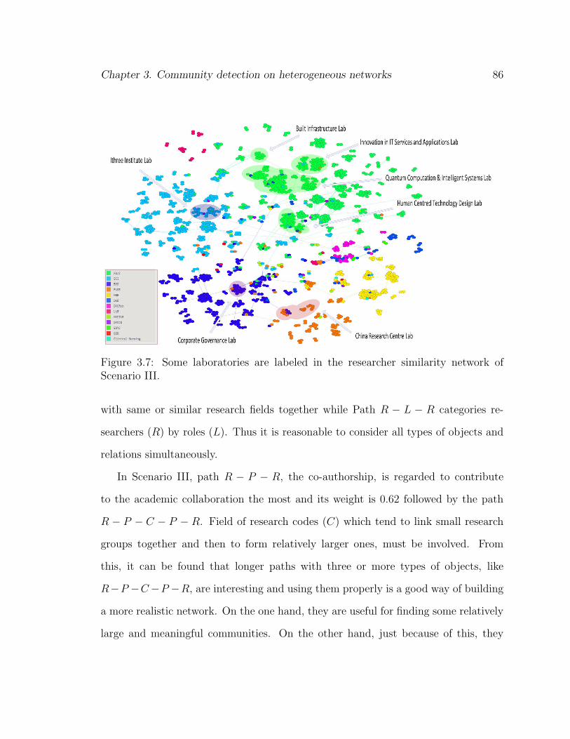
Chapter 3. Community detection on heterogeneous networks 86
Figure 3.7: Some laboratories are labeled in the researcher similarity network ofScenario III.
with same or similar research fields together while Path R − L − R categories re-
searchers (R) by roles (L). Thus it is reasonable to consider all types of objects and
relations simultaneously.
In Scenario III, path R − P − R, the co-authorship, is regarded to contribute
to the academic collaboration the most and its weight is 0.62 followed by the path
R − P − C − P − R. Field of research codes (C) which tend to link small research
groups together and then to form relatively larger ones, must be involved. From
this, it can be found that longer paths with three or more types of objects, like
R−P −C−P −R, are interesting and using them properly is a good way of building
a more realistic network. On the one hand, they are useful for finding some relatively
large and meaningful communities. On the other hand, just because of this, they
Chapter 3. Community detection on heterogeneous networks 87
cannot have a large weight; otherwise all objects are linked together. This conclusion
is also supported by the theory in Sun & Han (2012).
The other two paths (R − F − R and R − L − R) are of little importance and
can be ignored in the further research. The situation of academic collaboration at
UTS is better revealed by this scalar combination. Figure 3.7 is the researcher (R)
similarity network where researchers are colored by their faculties. The edge weights
between researchers are the collective similarities. It can be seen that the academic
collaboration groups are relatively larger than those in Scenario II. Meanwhile these
groups are meaningful. They are matched with the current laboratory setting of UTS
and some of them are labeled.
From the analysis above, it can be seen that it is necessary to consider multi-typed
relations and objects in investigating abstract concepts and the single relationships
and objects are insufficient for revealing the real situation. On the other hand, rela-
tionships (represented by semantic paths) have varying levels of importance. There-
fore, assessing them before clustering is of great necessity and the proposed method
for evaluating paths based on correlations is effective.
3.4.3 Community detection and validation
In this section, both Multiple Semantic-path Clustering and spectral clustering are
applied to detect communities on the heterogeneous UTS academic collaboration net-
work. Spectral clustering works on the researcher similarity matrix built by random-
walk. For Multiple Semantic-path Clustering, the researcher similarities are based on
the collective similarity which is from Scenario III and communities are detected by
the method proposed in Section 3.1.1. This chapter considers the UTS laboratory

Chapter 3. Community detection on heterogeneous networks 88
setting as a partition where laboratories are clusters and researchers who work in
these laboratories are objects in these clusters.
The clustering results generated by these methods are compared with the ground
truth, the UTS laboratory setting by Vector-Based Comparison (V-B Comparision)
and Normalized Mutual Information (NMI).
Table 3.4: Clustering validation
Comparative methods V-B Comparison NMI
Multi-path clustering vs. the lab setting 0.932 0.916
Spectral clustering vs. the lab setting 0.762 0.658
The comparative results are listed in Table 3.4 which shows that the clusters
generated by multi-path clustering are more similar to the laboratory setting than
spectral clustering as evidenced by the relatively high values in V-B Comparison
and NMI. This result also confirms that random-walk is not suitable to apply on
heterogeneous networks. The possible reasons for this are that 1) random-walk is
advantaged in finding large communities but weak in finding small communities where
vertices have fewer edges because the random moving decisions are made based on
probability; and 2) in heterogeneous networks, the probabilities of an agent moving
from one type of object to the other type objects should be different. Indeed, these
probabilities are often hard to measure or estimate.
This suggests that taking multi-typed relationships and objects into consideration
is necessary to analyze some abstract and hard-to-be-measured social phenomena.
This section also compares the quality of clusters of both methods by clustering
quality indices: Coverage, Performance and Modularity.

Chapter 3. Community detection on heterogeneous networks 89
Table 3.5: Clustering quality validation
Methods Coverage Performance Modularity
Multi-path clustering 0.865 0.792 0.783
Spectral clustering 0.812 0.723 0.792
According to Table 3.5, both Multiple Semantic-path Clustering and spectral clus-
tering perform well in community detection, achieving similar values of quality in-
dices. This suggests that compared with spectral clustering, the proposed Multiple
Semantic-path Clustering method is also an effective community detection method.
The reason why these methods get similar results in clustering quality indices is
that these quality indices evaluate clustering based on different researcher similarity
networks instead of the heterogeneous UTS academic collaboration network. The
network used in spectral clustering is built by random-walk while that used in the
proposed Multiple Semantic-path Clustering method is from the collective similarity.
Currently, these clustering quality indices are only applicable in homogenous net-
works. Thus, it is unreasonable to estimate the quality of community detection by
clustering quality indices alone and this is why this thesis involves a ground truth to
verify the effectiveness of the proposed multiple semantic-path clustering.
3.5 Contribution and discussion
Heterogeneous networks are a model to represent abstract social phenomena for cov-
ering multi-typed objects and relations. Use of multi-typed objects and relationships
results in the fact that detecting communities on heterogeneous networks must con-
sider objects and relations of different types simultaneously and also needs to assess

Chapter 3. Community detection on heterogeneous networks 90
the contributions of different relations to the abstract concepts accurately.
This chapter addresses Contribution 1 of this thesis as listed in Section 1.5 by
proposing a general model to identify communities on heterogeneous networks based
on semantic paths and matrix factorization.
Contribution 1, a novel community detection method, named Multiple Semantic-
path Clustering is proposed in Section 3.1. In the proposed method, relations are
represented by semantic paths and the weights of semantic paths are assessed by
correlations between each semantic path and a ground truth situation. Then a col-
lective similarity is calculated based on the combination of semantic paths and the
community structure can be identified by using matrix factorization theory.
The outcomes of the above stated method are compared with another robust
state-of-the-art method, spectral clustering. The results of the proposed method are
superior to that in terms of revealing the academic collaboration more accurately and
the quality of clusters is also very high in three indices: coverage, performance and
modularity.
The main issue with the results of the proposed Multiple Semantic-path Clus-
tering is that this method is applied on the academic collaboration at UTS which
is a relatively small dataset. Its effectiveness and efficiency should be tested in a
large dataset further in the future. Another limitation is that this method just finds
communities for the target object instead of all types, which means if users want to
find communities for all types of objects, this method will need to be executed many
times. Therefore, one research direction is to extend this method to find communities
for all types of objects in the same time.

Chapter 4
Determine the number of clustersby leaders
As is explained in the literature review (Sec. 2.2), determining the correct number of
clusters functions as an effective way of finding high-quality clusters. Although there
are many ways of achieving this (Fraley & Raftery 2002, Chiang & Mirkin 2010,
Maulik & Bandyopadhyay 2002, Lange et al. 2004), they are sensitive to the topolog-
ical features of networks. This chapter aims to overcome this weakness by proposing
a Leader Detection and Grouping Clustering (LDGC) method. The proposed method
is designed for both homogenous and heterogeneous networks to determine the num-
ber of clusters beforehand based on network topological features. This can support
Contribution 2 of this thesis which is to propose a method to determine the number
of clusters in both homogeneous and heterogeneous networks.
In social networks, communities are generally constituted by leaders and commu-
nity members simultaneously. Leaders are often regarded as more important than
others in terms of network connectivity because they are the core of communities and
the other objects are connected to each other via them. This phenomenon is also seen
in social science (Parkin 2013) in that a networked community is always formed by
91

Chapter 4. Determine the number of clusters by leaders 92
one or several leaders and their followers. These leaders often have many connections
with community members while community members are often connected via the
leaders. This gives rise to a close correlation between the number of community lead-
ers and the number of clusters. As long as leaders and their similarities are identified,
it is possible to know the number of clusters.
The proposed Leader Detection and Grouping Clustering method can distinguish
leaders from all objects based on their different topological features. Leaders not only
have more connections in clusters but also have a relationship to individuals in other
clusters. Degree-centrality and betweenness-centrality can reflect this characteristic.
Meanwhile, considering the situation that sometimes there are two or more leaders
in one potential group, this thesis proposes an algorithm to combine leaders when
they are close enough. Leaders who are similar should be grouped to form leader
groups. The number of leader groups is the number of communities. The proposed
Leader Detection and Grouping Clustering method can also detect communities in
both heterogeneous and homogeneous networks. After determining leader groups, the
remaining vertices are allocated into those groups which they are close to.
Finally, the proposed Leader Detection and Grouping Clustering method is val-
idated on the UTS heterogeneous academic collaboration network for determining
the number of clusters and detecting communities. To illustrate its effectiveness, this
chapter involves spectral clustering in a comparative experiment.
The rest of this chapter is organized as follows: Section 4.1 describes the pro-
posed Leader Detection and Grouping Clustering method followed by the experimen-
tal dataset in Section 4.3 and results in Section 4.4. The contribution and discussion
of the proposed method is given in Section 4.5.
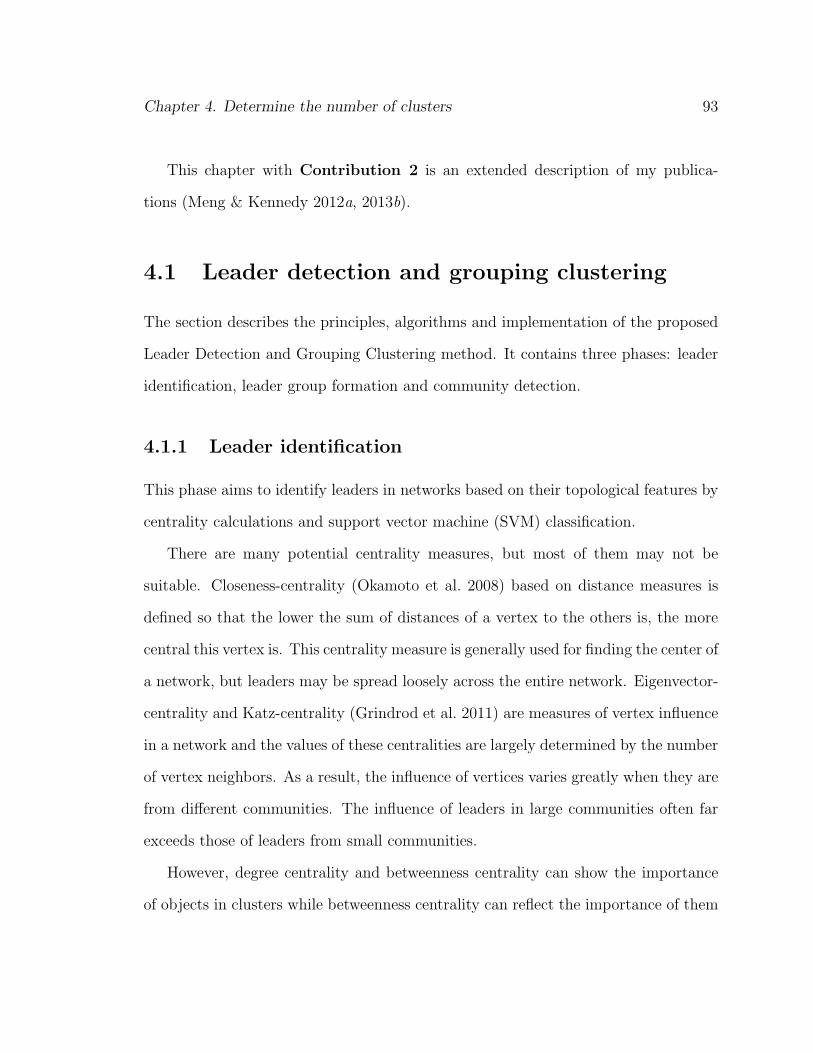
Chapter 4. Determine the number of clusters 93
This chapter with Contribution 2 is an extended description of my publica-
tions (Meng & Kennedy 2012a, 2013b).
4.1 Leader detection and grouping clustering
The section describes the principles, algorithms and implementation of the proposed
Leader Detection and Grouping Clustering method. It contains three phases: leader
identification, leader group formation and community detection.
4.1.1 Leader identification
This phase aims to identify leaders in networks based on their topological features by
centrality calculations and support vector machine (SVM) classification.
There are many potential centrality measures, but most of them may not be
suitable. Closeness-centrality (Okamoto et al. 2008) based on distance measures is
defined so that the lower the sum of distances of a vertex to the others is, the more
central this vertex is. This centrality measure is generally used for finding the center of
a network, but leaders may be spread loosely across the entire network. Eigenvector-
centrality and Katz-centrality (Grindrod et al. 2011) are measures of vertex influence
in a network and the values of these centralities are largely determined by the number
of vertex neighbors. As a result, the influence of vertices varies greatly when they are
from different communities. The influence of leaders in large communities often far
exceeds those of leaders from small communities.
However, degree centrality and betweenness centrality can show the importance
of objects in clusters while betweenness centrality can reflect the importance of them

Chapter 4. Determine the number of clusters 94
out of clusters. For example, in a company, managers can be naturally considered
as leaders. They not only need to communicate with his or her team members but
also need to talk to other managers. For team members, they generally interact
with their managers or other members in the same team instead of communicating
with other managers. Degree-centrality and betweenness-centrality can capture this
feature accurately. As a result, they are empirically considered as major indices to
reflect the topological features of networked objects in both local and global levels.
The following are the definitions of these centralities which are reviewed in Section 2.3.
1. Degree centrality is the simplest centrality which counts the number of links
from one node, say v to the others.
CD(v) = degree(v) (4.1.1)
2. Betweenness centrality describes that the more central one vertex is, the
more edges and vertices are joined by it. It is the ratio between the number of
short paths from starting point s to ending point e passing through v to not
passing through v.
CB(v) =∑ pse(v)
pse(4.1.2)
The calculation of betweenness-centrality in this chapter refers to the approach in Bran-
des (2001). It is a well-known algorithm requiring O(|V ||E|) time for unweighted net-
works and O(|V ||E|+ |V |2 log |V |) time for weighted graphs, where |V | is the number
of vertices and |E| is the number of edges in the network.

Chapter 4. Determine the number of clusters 95
Values of degree-centrality and betweenness-centrality often have different ranges.
For classification and visualization, the values of these two centralities are normal-
ized into the same range by two different ways. For degree-centrality, values are
linearly scaled into [0, 1] because the ranges of degree-centrality values is narrow. For
betweenness-centrality, values of this centrality have a wide range and the distribu-
tion of these values are not even with a long tail. This chapter applies log function
to scale these values into a small range and then linearly normalized these processed
values into [0, 1].
Table 4.1: A sample of new built dataset
VertexID Degree centrality Betweenness-centrality
10001 0.0417 0
10002 0.0833 0
10003 0.1251 0.0084
Leaders are identified through their special topological features which are revealed
by the combination of degree-centrality and betweenness-centrality. Leader identifica-
tion can be viewed as a binary classification problem (refer to Section 2.3.3) because
there are just two classes: leaders and community members. In this chapter, this
binary classification problem is addressed by Support Vector Machine (Chang & Lin
2011) which is a widely applied binary classification and the kernel function is chosen
as Gaussian kernel function which can detect clusters with an irregular boundary.
KG(vi, vj) = exp
(−||vi − vj||2
σ2
)(4.1.3)
After the degree-centrality and betweenness-centrality calculations, this chapter
builds a new dataset which contains vertexID, degree-centrality and betweenness-
centrality. The dataset is randomly divided into three sub datasets: a training dataset

Chapter 4. Determine the number of clusters 96
(300 researchers), a cross validation dataset (300 researchers) and a test dataset (835
researchers). In the training dataset, vertices are labeled as leaders or not. The reason
for setting up relatively small training and a cross validation datasets is to evaluate
the effectiveness of the proposed method in detecting leaders. The cross validation
dataset is for determining the parameters of the Gaussian kernel function based on
the error rate.
4.1.2 Leader group formation
It is noticeable that the number of leaders is often not the number of clusters unless
the aim is to find small, cohesive cliques. In most cases, the number of leaders
outnumbers the number of clusters because one community is very likely to have
more than one leader, especially in large communities. For acquiring the “correct”
number of clusters, leaders with a close relationship should be grouped and then
the number of leader groups is the number of clusters. As is shown in the example
in Figure 4.1, there are three communities: group A, group B and group C. Based
on the values of degree-centrality and betweenness centrality, leader 1 and leader 2
in group A have the same importance. Consequently, the number of leaders is four
because leader 1 and leader 2 are very close and they have 6 common neighbors. So
after leaders are found, the next step is to look into their similarities. In this phase,
similar leaders are allocated to the same leader group; otherwise they are put into
different leader groups.
Another usage of leader groups is to control the size of clusters. For example,
in order to achieve balanced clusters which means clusters having similar numbers
of objects, large leader groups can be separated into small ones while small groups

Chapter 4. Determine the number of clusters 97
Figure 4.1: An example of why leaders should be grouped
can be integrated into a larger one. This allows LDGC to satisfy more complex user
requirements on the size of clusters.
Leader groups are built based on their similarities. This chapter proposes a het-
erogeneous network oriented similarity measure which is designed to make full use of
topological features of heterogeneous networks. The similarities among objects are
acquired based on the number and the length of semantic paths, and the number
of paths in each semantic path. Given vertices x and y in a heterogeneous network
G, their semantic paths are represented by set Pxy. The similarity between them is
defined as
Sim(x, y) =1
|Pxy|∑i∈Pxy
1
len(i)
2Nxy(i)
Nx(i) +Ny(i)(4.1.4)
where |Pxy| is the number of elements in set Pxy. For a semantic path i, Nxy(i) is the
number of paths in this type between x and y. Nx(i) andNy(i) are the number of paths

Chapter 4. Determine the number of clusters 98
Figure 4.2: The working process of community detection by Leader Detection andGrouping Clustering. Circles are vertices and LGi refers to leader groups. Thesimilarity between vertices and leader groups are calculated and vertices are allocatedto those leader groups with highest similarity.
in semantic path i. The length of semantic path i is marked as len(i). For example,
the length of semantic path A−B − C −B −A is four. In heterogeneous networks,
length is an important topological features of a semantic path. Long semantic paths
mean far distances between objects and should be assigned small weights (Sun & Han
2012). This is the reason why length is taken into account.

Chapter 4. Determine the number of clusters 99
4.1.3 Community detection
After building leader groups, the proposed Leader Detection and Grouping Cluster-
ing method can detect communities in heterogeneous networks based on these groups.
Given a heterogeneous network G = (V,E), there are k leader groups (LG1, . . . , LGk).
The remaining vertices are allocated to leader groups based on their similarities with
leader groups. Figure 4.2 illustrates the working process of the proposed Leader De-
tection and Grouping Clustering method in community detection. It can be seen that
similarities between the rest vertices and leader groups are calculated and then these
vertices are allocated to these most similar ones. The ways of measuring similarities
between vertices and leader groups are many. In this chapter, the similarity measure
is based on shortest-path. Vertex v (v ∈ V ) is allocated to leader group LGi, if the
average shortest-path distance of v to the leaders in LGi is shorter than to the leaders
in the other leader groups.
Algorithm 4.1 Algorithm for community detection by Leader Detection and Group-ing Clustering
Initialization:Set LG1, . . . , LGk as array;Set CLS1, . . . , CLSk as array;
Iteration:1: for v = 1; v <= |V |; v ++ do2: t = 1;3: for i = 1; i <= k; i++ do4: if AvgShortPath(v, LGi) < AvgShortPath(v, LGt) then5: t = i;6: end if7: end for8: put(v, CLSt);9: end for
Algorithm 4.1 describes the method for community detection by the proposed
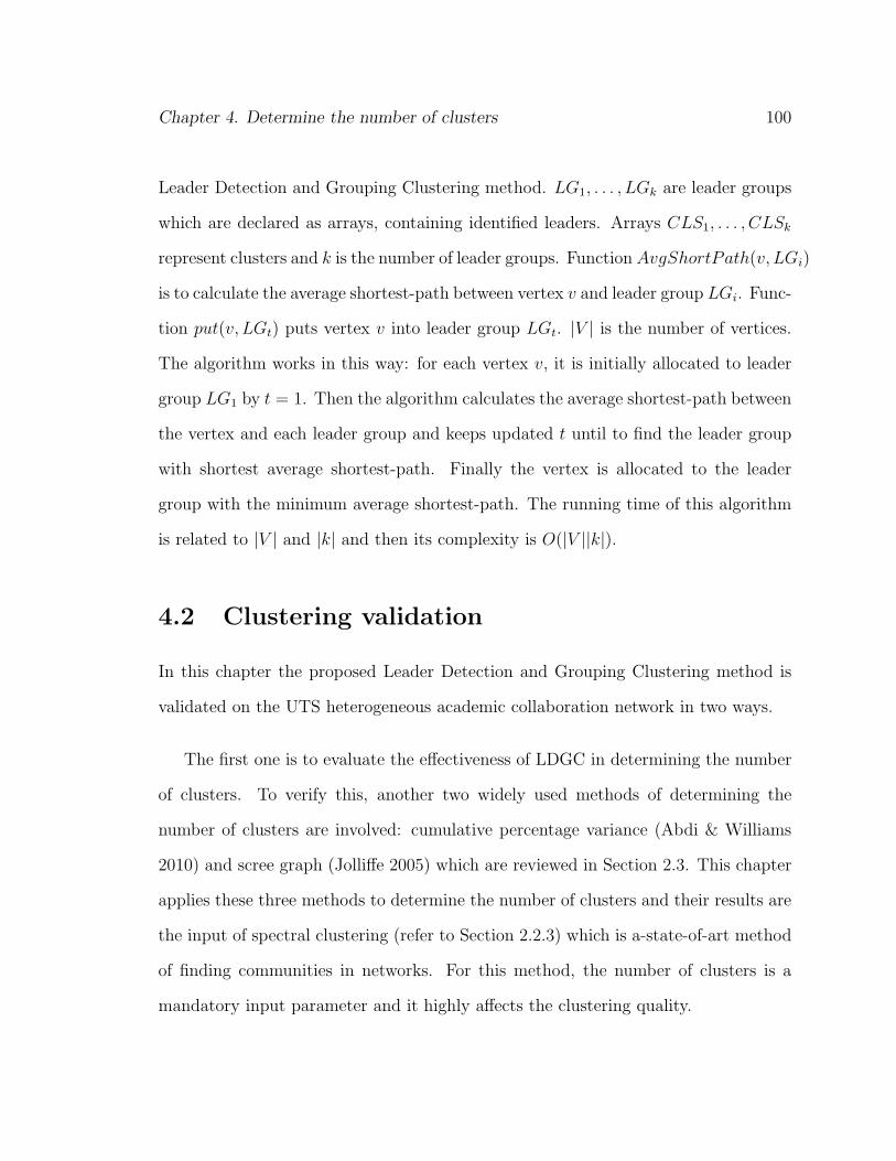
Chapter 4. Determine the number of clusters 100
Leader Detection and Grouping Clustering method. LG1, . . . , LGk are leader groups
which are declared as arrays, containing identified leaders. Arrays CLS1, . . . , CLSk
represent clusters and k is the number of leader groups. Function AvgShortPath(v, LGi)
is to calculate the average shortest-path between vertex v and leader group LGi. Func-
tion put(v, LGt) puts vertex v into leader group LGt. |V | is the number of vertices.
The algorithm works in this way: for each vertex v, it is initially allocated to leader
group LG1 by t = 1. Then the algorithm calculates the average shortest-path between
the vertex and each leader group and keeps updated t until to find the leader group
with shortest average shortest-path. Finally the vertex is allocated to the leader
group with the minimum average shortest-path. The running time of this algorithm
is related to |V | and |k| and then its complexity is O(|V ||k|).
4.2 Clustering validation
In this chapter the proposed Leader Detection and Grouping Clustering method is
validated on the UTS heterogeneous academic collaboration network in two ways.
The first one is to evaluate the effectiveness of LDGC in determining the number
of clusters. To verify this, another two widely used methods of determining the
number of clusters are involved: cumulative percentage variance (Abdi & Williams
2010) and scree graph (Jolliffe 2005) which are reviewed in Section 2.3. This chapter
applies these three methods to determine the number of clusters and their results are
the input of spectral clustering (refer to Section 2.2.3) which is a-state-of-art method
of finding communities in networks. For this method, the number of clusters is a
mandatory input parameter and it highly affects the clustering quality.
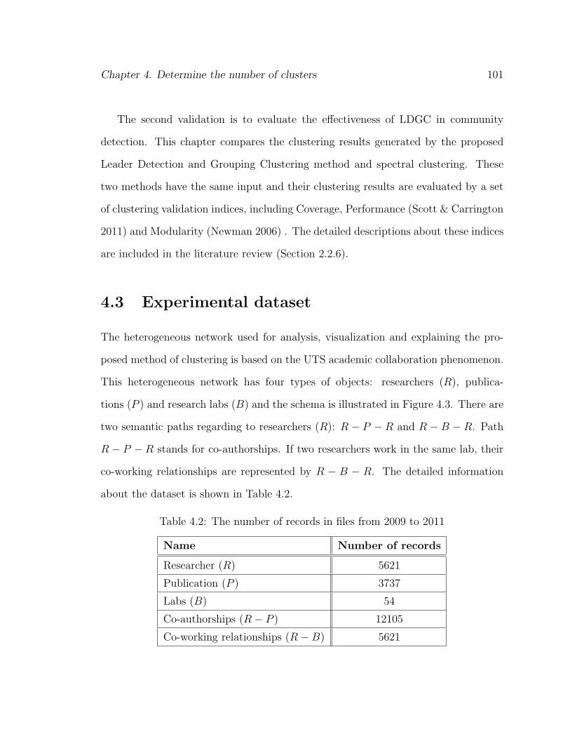
Chapter 4. Determine the number of clusters 101
The second validation is to evaluate the effectiveness of LDGC in community
detection. This chapter compares the clustering results generated by the proposed
Leader Detection and Grouping Clustering method and spectral clustering. These
two methods have the same input and their clustering results are evaluated by a set
of clustering validation indices, including Coverage, Performance (Scott & Carrington
2011) and Modularity (Newman 2006) . The detailed descriptions about these indices
are included in the literature review (Section 2.2.6).
4.3 Experimental dataset
The heterogeneous network used for analysis, visualization and explaining the pro-
posed method of clustering is based on the UTS academic collaboration phenomenon.
This heterogeneous network has four types of objects: researchers (R), publica-
tions (P ) and research labs (B) and the schema is illustrated in Figure 4.3. There are
two semantic paths regarding to researchers (R): R − P − R and R − B − R. Path
R − P − R stands for co-authorships. If two researchers work in the same lab, their
co-working relationships are represented by R − B − R. The detailed information
about the dataset is shown in Table 4.2.
Table 4.2: The number of records in files from 2009 to 2011
Name Number of records
Researcher (R) 5621
Publication (P ) 3737
Labs (B) 54
Co-authorships (R− P ) 12105
Co-working relationships (R− B) 5621

Chapter 4. Determine the number of clusters 102
Figure 4.3: The schema of the experimental heterogeneous network.
4.4 Experiment
This section validates the effectiveness of the proposed Leader Detection and Group-
ing Clustering method on the UTS heterogeneous academic collaboration network
in determining the number of clusters and community detection respectively. The
network contains three types of vertices: Researchers (R), Papers (P ) and Labs (L)
and two types of edges: publishing and belonging to. The weight of edges is 1.
4.4.1 Leader identification
The experimental heterogeneous network is the UTS heterogeneous academic collab-
oration network (Figure 4.3). The degree and betweenness centrality of researchers
in the UTS heterogeneous academic collaboration network is calculated by referring
to the Equations (4.1.4) and (4.1.2) respectively. In the experiment, degree and be-
tweenness centrality have different value ranges. Degree centrality ranges from 1 to
24 and betweenness centrality from 0 to 95127.57. For adjusting these values into the
same range, values of both centralities are rescaled into [0, 1] (refer to Section 4.1.1).
After normalization, the distributions of degree and betweenness centrality of
Chapter 4. Determine the number of clusters 103
Figure 4.4: The distribution of researcher degree centrality
Figure 4.5: The distribution of researcher betweenness centrality

Chapter 4. Determine the number of clusters 104
Figure 4.6: The result of leader detection by SVM in R. Triangles and circles aredata points from two clusters. Circles stand for leaders and triangles are commu-nity members. Solid triangles and circles are support vectors of these two clustersrespectively.
researchers (R) are shown in Figure 4.4 and Figure 4.5 respectively. It can be seen
from these two figures that these two distributions display a long tail. This means
these two distributions are uneven: most researchers (R) have very small values of
degree and betweenness centrality and the gap between small values and large values
are very huge.
Leader detection in this chapter is a binary classification problem which is ad-
dressed by Support Vector Machine (SVM). This experiment builds a new dataset
which contains vertexID, degree-centrality and betweenness-centrality. The dataset
is randomly divided into three sub datasets: a training dataset (300 researchers), a

Chapter 4. Determine the number of clusters 105
cross validation dataset (300 researchers) and a test dataset (835 researchers). In the
training dataset, laboratory directors are considered as leaders and they are labeled as
1 while the other researchers (R) are labeled as 0. The scale parameter σ of Gaussian
kernel function (Equation (4.1.3)) is set as 0.45 based on the cross validation dataset
through error rate. After classification with a training error rate as 0.330865 and 94
support vectors, leaders with high similarities are combined into leader groups. This
experiment calculated the similarities between leaders referring to Equation (4.1.4).
Leaders are connected to their most similar neighbors to build a similarity network
if they are connected in both semantic paths, R − B − R and R − P − R. The un-
connected sub networks are leader groups. After leader combination, there are 206
leader groups and this is the number of clusters of this heterogeneous network.
4.4.2 Community detection
This section verifies the effectiveness of the proposed leader based community detec-
tion method in determining the number of clusters and in community detection.
In determining the number of clusters, the verifying process is based on the idea
that an accurate number of clusters can give rise to a high quality clustering. In this
chapter, the number of clusters of the heterogeneous networks is determined by three
approaches: cumulative percentage variance, scree graph and the proposed Leader
Detection and Grouping Clustering method. For cumulative percentage variance, the
threshold is chosen as 98% empirically. For scree graph the biggest slop is chosen
as the separating pointing of selected and unselected eigenvalues. Section 4.4.1 has
explained the way of determining the number of clusters by LDGC. The other two
methods determine the number of clusters through the structure of the researcher

Chapter 4. Determine the number of clusters 106
Figure 4.7: The eigenvalues of the random-walk Laplacian matrix.
similarity matrix which is generated by random walk. For The numbers of clusters
determined by these three methods are 206, 298 and 812 respectively. Spectral clus-
tering is applied with these three numbers of clusters and the clustering results are
shown in Table 4.3.
Table 4.3: Clustering results by spectral clustering
Methods Cumulative percentage Scree graph LDGC
variance
Clusters 298 812 206
Modularity 0.803 0.771 0.884
Coverage 0.822 0.803 0.876
Performance 0.784 0.782 0.889
It can be seen that the number of clusters determined by LDGC results in the

Chapter 4. Determine the number of clusters 107
best clustering quality and it achieve highest values in Modularity (0.884), Cover-
age (0.876) and Performance (0.889) followed by Cumulative percentage variance (Mod-
ularity (0.803), Coverage (0.822) and Performance (0.784)) and Scree graph (Modu-
larity (0.771), Coverage (0.803) and Performance (0.782)).
Table 4.4: Clustering results by spectral clustering and LDGC
Methods Spectral clustering LDGC
Clusters 206 206
Modularity 0.884 0.912
Coverage 0.876 0.908
Performance 0.889 0.932
In validating the effectiveness of Leader Detection and Grouping Clustering method
in community detection, both spectral clustering and LDGC have the same number
of clusters as an input which is determined by the proposed method in this chapter.
The clustering results generated by these two methods are compared by three com-
munity detection indices: Modularity, Coverage and Performance in Table 4.4. It can
seen from this table that the proposed LDGC method outperform spectral clustering
because it achieves higher values in these three indices than spectral clustering.
4.5 Contribution and discussion
The literature review of community detection shows that for most clustering methods,
accurate cluster numbers are of great importance to achieve a high-quality clustering.
However, determining the number of clusters before clustering is a challenge for both
homogeneous and heterogeneous network analysis.
This chapter addresses Contribution 2 of this thesis as listed in Section 1.5 by
Chapter 4. Determine the number of clusters 108
proposing a Leader Detection and Grouping Clustering to address this problem and
it is applicable for both homogeneous and heterogeneous networks. This method is
based on the social theory that a close connected community is constituted by one or
several leaders and their followers to investigate the different topological features of
group leaders and members in networks.
The proposed Leader Detection and Grouping Clustering method can distinguish
leaders from all objects based on their different topological features. Leaders not only
have more connections in clusters but also have a relationship to individuals in other
clusters. Degree-centrality and betweenness-centrality can reflect this characteristic.
Meanwhile, considering the situation that sometimes there are two or more leaders
in one potential group, this thesis proposes an algorithm to combine leaders when
they are close enough. Leaders who are similar should be grouped to form leader
groups. The number of leader groups is the number of communities. The proposed
Leader Detection and Grouping Clustering method can also detect communities in
both heterogeneous and homogeneous networks. After determining leader groups, the
remaining vertices are allocated into those groups which they are close to.
The proposed LDGC method is verified in two aspects: determining the number
of clusters and detecting communities. In the former aspect, the number of clusters
determined by LDGC is more accurate than cumulative percentage variance and
scree graph because spectral clustering with the number of clusters from LDGC can
achieve better clustering. In the latter aspect, LDGC is more effective than spectral
clustering in community detection. The clustering result of LDGC is better than
spectral clustering with accurate number of clusters determined by LDGC in terms
of Modularity, Coverage and Performance.

Chapter 4. Determine the number of clusters 109
For the proposed Leader Detection and Grouping Clustering method, the strategy
of identifying leaders can be improved. The experiment suggests that the error rate of
identifying leaders is high because the proposed method just applies degree-centrality
and betweenness-centrality to distinguish leaders and community members. It could
be possible that these two centralities may be insufficient to achieve this and other
topological features should be involved. Another limitation of this chapter is that the
laboratory directors are considered as leaders of communities and the SVM classifier
is trained based on this. In fact, some managers in companies or universities are not
leaders of communities. For example, department managers may have a close connec-
tion with project managers rather than all the staffs that they supervise. Training
the classifier by managers may give rise to biased results.

Chapter 5
Network evolution-based linkprediction
Link prediction is a fundamental question of heterogeneous network analysis. This
chapter aims to address it by proposing a novel link prediction method named Net-
work Evolution-based Link Prediction (NELP) which is designed for heterogeneous
networks. The major innovation of this method is to model vertex activeness by
their evolving patterns shown in network evolution so as to improve link prediction
accuracy.
Predicting whether two vertices in networks will develop a new connection or
maintain their current connection is mainly based on their “distance”. This means
the closer two vertices are, the higher possibility they will be connected in the future.
However, there are some exceptions that some vertices with a far distance may de-
velop a connection among them while some vertices with a close distance may not be
connected in the future. These exceptions are the main reason for failing to achieve
high link prediction accuracy.
Through observations and social theory (Carrington et al. 2005), different objects,
110

Chapter 5. Network evolution-based link prediction on heterogeneous networks 111
particularly humans, displayed different tendency towards developing their connec-
tions. Active ones tend to have more new connections or strengthen their current
connections in a short timeslot while stable ones prefer to maintain their existing
connections. Another interesting phenomenon is that objects have different capaci-
ties of connections. For examples, extroverted people generally have more friends than
the introvert. All these features can be acknowledged and extracted from network
evolutionary process which means that treating objects individually and capturing
their own evolutionary tendency are necessary to improve the accuracy of link pre-
diction. This is the reason why this chapter considers network evolution instead of a
single network snapshot for making link prediction.
Traditional link prediction methods are based on similarity measures. The princi-
ple of these methods is that they use similarity measures to calculate the similarities
between vertices and predict that those links of r leading highest similarities will
appear in the future. Indeed, it is hard to determine the value of r. The proposed
can overcome this by involving matrix decomposition theory to exclude noisy data.
The chapter is organized as follows: Section 5.1 describes the proposed Network
Evolution-based Link Prediction method followed by the experimental dataset and
results in Sections 5.2 and 5.3. Section 5.4 presents the contribution and discussion
of this chapter.
This chapter, describing Contribution 3, is an extended description of my pub-
lication (Meng & Kennedy n.d.).

Chapter 5. Network evolution-based link prediction on heterogeneous networks 112
5.1 Methodology
This section describes how to model vertex activeness followed by the descriptions
about the proposed Network Evolution-based Link Prediction method and evaluation.
5.1.1 Modeling vertex activeness
This section first describes how to model network evolution followed by determining
vertex activeness. Most social networks keep changing due to their dynamic nature.
But in a particular time point, these networks are static. From this perspective,
it is reasonable to model the evolutionary process of a dynamic network by using
a set of static networks captured at different time points to represent the network
evolutionary process. The closer the time points are, the more accurate the network
evolution can be modeled.
Definition 5.1. Given a heterogeneous network G = (V,E), there are n types of
object (V = {V1, . . . , Vn}) and m types of edges (E = {E1, . . . , Em}). The process
of the network evolution can be represented by a series of snapshots of this network,
Ω = (Gt1 , . . . , Gtn). These snapshots are captured at different time points, t1, . . . , tn.
Among them, Gti = (Vti , Eti) represents the network at ti. Then the link prediction
problem is to predict Gtn+1 based on these networks (Gt1 , . . . , Gtn).
This chapter determines vertex activeness based on their evolving patterns which
measures how fast vertices change their connections. Two speed indices are proposed
in this chapter to capture vertex evolving patterns on heterogeneous networks and
they are Neighborhood Changing Velocity (NCVelocity) and Neighborhood Changing
Accelerated Velocity (NCAVelocity). Neighborhood Changing Velocity (NCVelocity)
refers to a vertex speed of changing neighbors and the NCVelocity of vertex v (v ∈ V )

Chapter 5. Network evolution-based link prediction on heterogeneous networks 113
at ti is defined as
NCV elocity(v, ti) =1
ti − ti−1
· |neighbor(v, ti) ∩ neighbor(v, ti−1)||neighbor(v, ti) ∪ neighbor(v, ti−1)| (5.1.1)
where neighbor(v, ti) represents the neighbor set of vertex v at ti and |neighbor(v, ti)∩neighor(v, ti−1)| is the number of common neighbors of vertex v at times ti and ti−1.
Neighborhood Changing Accelerated Velocity (NCAVelocity), the accelerated speed
of NCVelocity, represents the changes of NCVelocity over time and NCAVelocity of
vertex v at ti is defined as
NCAV elocity(v, ti) =NCV elocity(v, ti)−NCV elocity(v, ti−1)
ti − ti−1
(5.1.2)
With these two indices, it is possible to investigate into how vertices evolve over
time. These evolving patterns are about vertex preference of developing new connec-
tions or maintaining their existing connections. Through observations, the changing
patterns can be categorized into four groups: guest vertices, active vertices, stable
vertices and regular vertices and in terms of behaviors and activeness. Followings are
the detailed descriptions about these four groups.
Guest vertices
Guest vertices means those vertices that fail to stay in networks permanently.
They may stay in networks for a short time and then disappear or they jump
in and out networks from time to time. In link prediction, these vertices can
be considered as noise data as their behaviors are hard to be predicted. In this
chapter, those vertices who fail to appear in one or more collected snapshots of
networks are considered as guest vertices.

Chapter 5. Network evolution-based link prediction on heterogeneous networks 114
Active vertices
Vertices in this group are very vigorous and they are the main contributors
to make networks keep changing. During network evolution, their connections
are growing fast and they also can maintain a large number of connections.
Meanwhile a connection of two isolated groups may often start from them.
This chapter regards these vertices that have positive NCAVelocity at every
time point as active vertices. This means these vertices not only have more
connections with others but also their speeds of having new connections are
increasing.
Stable vertices
Stable vertices tend to maintain their existing relationships (NCV elocity(v, ti) =
1, i ∈ (1, . . . , n)) as time goes. They may be viewed as inactive vertices because
they contribute little to the network evolution.
Regular vertices
The remaining vertices are defined as regular vertices. These vertices with
moderate speeds of changing connections are allocated in this category. In fact,
most vertices are in this category.
Due to the fact that vertices have different evolving preferences, it is necessary to
classify them before predicting links. In the task of link prediction, adopting different
strategies to handle vertices in different groups can not only increase the accuracy
of link prediction but can also improve the efficiency. For two active vertices, even
though they are far from each other, the possibility of them to develop a new link

Chapter 5. Network evolution-based link prediction on heterogeneous networks 115
is high. For two stable vertices, even if they are near to each other, they are very
unlikely to develop a connection. The evolving patterns of guest vertices are often
unpredictable. This thesis treats them as noisy data and excludes them from link
prediction.
5.1.2 Network Evolution-based link prediction
Most link prediction methods in networks are based on distances which are calculated
by similarity measures. Generally, if two vertices are close in networks, they have a
higher possibility of developing a connection between them in the future. If they are
far apart, the possibility of developing a connection between them is low. However,
when the process of network evolution is considered, it can be seen that vertices have
different velocities of changing their connections. Some of them are fast while some
of them are low. The proposed Network Evolution-based Link Prediction method is
designed to consider vertex evolving patterns to improve link prediction accuracy and
is compatible with different heterogeneous network similarity measures.
The proposed Network Evolution-based Link Prediction method is designed to
work on a similarity matrix of heterogeneous networks which can be built by different
heterogeneous similarity measures. This means the proposed link prediction method
can improve accuracies of link prediction methods based on different similarity mea-
sures. Consider a similarity matrix S, sij is the similarity between vertex i and j.
The proposed Network Evolution-based Link Prediction method integrates similarity
matrix S with vertex involving patterns and redefines it as
P = ZSZT (5.1.3)

Chapter 5. Network evolution-based link prediction on heterogeneous networks 116
where Z = (z1, . . . , z|V |)T is a vector containing vertex Neighborhood Changing Ve-
locity where |V | is the number of vertices, zi = NCV elocity(i, tn) and 1 ≤ i ≤ |V |.Then the link prediction matrix P can be written as P = UDV T by the singular
value decomposition (SVD). Matrices U and V are orthogonal matrices and D is a
diagonal matrix of singular values σ1 > σ2 > . . . > σR > 0. According to truncated
matrix theory,
P ≈ UkDkVTk (5.1.4)
where Uk and Vk comprise the first k columns of U and V , and D is the k × k
principal submatrix of D. As a result, a matrix of predicted links can be written as
P ′ = UkDkVTk which contains the main features of matrix P . For link prediction,
if puv > 0 where puv is an element in link prediction matrix P , there will be a
connection between vertices u and v; otherwise, vertices u and v will not be connected
in the future.
There are two types of link prediction: new-link prediction and all-link prediction.
The problem of new-link prediction aims to find those links that do not exist in
current networks but will appear in the future. For example, in a friendship network,
predicting new links means whether two persons will become friends in the future.
For link prediction matrix P , if puv > 0 and vertices u and v are not connected
in the current network, it is predicted to develop a new link between them in the
future. The problem of all link prediction aims not only to find new links but also to
predict whether two vertices will maintain their existing links. For example, in a co-
authorship network, all link prediction aims to not only find links that do not exist in
the current network and will appear in the future, but also predicts whether current
links will be maintained in the future. For link prediction matrix P , if puv > 0,

Chapter 5. Network evolution-based link prediction on heterogeneous networks 117
it is predicted to have a link between them in the future. The propose Network
Evolution-based Link Prediction method in this chapter can work on both of them.
According to the vertex evolving analysis in the previous section, it can be seen that
both active and regular vertices tend to have new connections. Stable ones keep their
existing connections and guest ones are noise. In this way, when predicting new links
by Equation (5.1.4), k is the number of active vertices plus the number of regular
vertices. When predicting all links, k is the total number of active, regular and stable
vertices. The complexity of the proposed Network Evolution-based link prediction
method is constituted by vertex activeness calculation O(|V ||t|) and SVD based link
prediction O(|V |3) (Skillicorn (2007)) where |V | is the number of vertices and |t| isthe number of time slots. Thus the overall complexity is O(|V |3).
5.1.3 Evaluation
This chapter evaluates the proposed Network Evolution-based Link Prediction method
on the UTS heterogeneous academic collaboration network for predicting new links
and all links. This chapter applies three similarity-based link prediction methods:
random-walk, SimPath (the descriptions about these two similarity measures can be
found in the literature review of this thesis) and the proposed semantic-path simi-
larity (Section 4.1.2) of this thesis. Then the proposed link prediction method works
on the link prediction matrices generated by these three methods for improving link
prediction accuracy.

Chapter 5. Network evolution-based link prediction on heterogeneous networks 118
Figure 5.1: The schema of the heterogeneous academic collaboration network at UTS.
5.2 Experimental dataset
The experimental network of link prediction is a heterogeneous academic collabora-
tion network at UTS. In this network there are three types of objects: researchers (R),
publications (P ) and FoR codes (C). Researchers (R) are connected to their publi-
cations (P ) while publications (P ) are linked to research domains (C). The schema
of this heterogeneous network is illustrated in Figure 5.1.
Table 5.1: The experimental dataset from UTS
Year 2006 2007 2008 2009 2010 2011
Researchers 2763 2972 3148 3231 3548 3592
Publications 1941 1971 2010 1985 2047 2052
FoR Codes 584 584 584 584 584 584
Res-Pub links 5389 5739 5981 5893 6336 6963
Pub-FoR links 4562 4279 4632 4341 5457 5358
The datasets contains researcher (R), publication (P ), FoR codes (C), researcher-
publication links and publication-FoR codes links of each year from 2006 to 2011 (Ta-
ble 5.1). In the chapter, datasets from 2006 to 2010 are used to summarize the
evolution of the heterogeneous academic collaboration network which link prediction
is based on and the 2011 data is used to estimate the link prediction accuracies.

Chapter 5. Network evolution-based link prediction on heterogeneous networks 119
5.3 Experimental results
This section describes the application of proposed Network Evolution-based Link
Prediction method on a real-world dataset. This method is applied to predict links
of UTS academic collaboration in 2011 based on the data from 2006 to 2010 and the
real situation in 2011 is used to verify the accuracy of the proposed link prediction
method.
5.3.1 Modeling vertex activeness evolution
As discussed in the previous section, network evolution can be represented by a set of
network snapshots. This chapter models the process of network evolution from 2006
to 2010 and builds one network for each year. The summary information of these
networks are listed in Tab. 5.2. It clearly illustrates that the academic collaboration
network is a mature network. The numbers of vertices and edges grow annually, but
the density of network (|E|/|V |2) keeps almost the same. Meanwhile, the network is
quite sparse because its density is very low.
Table 5.2: Statistics of the academic collaboration network from 2006 to 2011
Year Vertices Edges Density of Networks
2006 5288 9951 0.00035
2007 5527 9658 0.00032
2008 5742 10613 0.00032
2009 5800 10234 0.00031
2010 6159 11793 0.00031
2011 6228 12321 0.00032

Chapter 5. Network evolution-based link prediction on heterogeneous networks 120
5.3.2 Determining vertex evolving patterns
The core step of increasing the accuracy of link prediction is to capture vertex evolv-
ing patterns. These patterns are based on their activeness which are measured by
two proposed evolving speeds: NCVelocity and NCAVelocity. According to Equa-
tions (5.1.1) and (5.1.2), these two speeds of researchers in the UTS heterogeneous
academic collaboration are calculated at years 2007, 2008, 2009 and 2010. Then re-
searchers are categorized into four groups: guest, active, regular and stable vertices
based on the definitions in Section 5.1.1. It can be seen in Table 5.3 that most vertices
are regular vertices, followed by stable vertices, guest vertices and active vertices.
Table 5.3: Categories of vertices
Category Vertex numbers Percentage
Active vertices 359 10.4%
Regular vertices 1713 49.6%
Stable vertices 854 24.7%
Guest vertices 526 15.3%
5.3.3 Link prediction
This section evaluates the proposed link prediction method on the UTS academic
collaboration network. The target object type is researchers (R) and the relationship
between them is co-authorship. The proposed Network Evolution-based Link Predic-
tion is applied to predict new links and all links respectively in 2011 based on the
network evolution from 2006 to 2010.
This experiment applies random walk and PathSim to predict links respectively.
These two methods calculate similarities of researchers (R) and the r leading highest

Chapter 5. Network evolution-based link prediction on heterogeneous networks 121
similarities are predicted to happen in the future. As is shown in Table 5.1, the number
of edges grows steadily during the five years. There are 6336 edges in 2010 and then it
can be safely assumed that there are 6800 edges in 2011. As a result, for predicting all
links, the first leading 6800 largest similarities of researchers are predicted to appear
while for predicting new links, the first leading 464 (6800 - 6336) largest similarities
of researchers who are not connected before are predicted to connect.
This experiment compares the accuracies of random-walk, SimPath and the pro-
posed semantic-path similarity with and without the proposed link prediction method
and the comparative results are listed in Table 5.4. It can be seen that the proposed
semantic-path similarity measure outperforms random walk and SimPath in both
types of link prediction. For predicting new links, the accuracy of the proposed
semantic-path similarity is 0.62 followed by Simpath (0.51) and random walk (0.26).
For predicting all links, the accuracy of the proposed semantic-path similarity is 0.71
followed by SimPath (0.53) and random walk (0.34). This demonstrates that the pro-
posed semantic-path based similarity measure works better to measure the similarities
on heterogeneous networks than random walk and SimPath.
Table 5.4: Link prediction accuracy comparison.
Link prediction methods New Link All Link
prediction accuracy prediction accuracy
Random-walk 0.26 0.34
Random-walk with NELP 0.31 0.45
SimPath 0.51 0.53
SimPath with NELP 0.54 0.63
Semantic-path similarity 0.62 0.71
Semantic-path similarity with NELP 0.69 0.82

Chapter 5. Network evolution-based link prediction on heterogeneous networks 122
When integrating the proposed link prediction method with these three similarity
measures, the accuracies of new-link prediction and all-link prediction are improved
significantly. For predicting new links, the accuracies of random walk, SimPath and
the proposed semantic-path similarity increases from 0.26 to 0.31, from 0.51 to 0.54
and from 0.62 to 0.69 respectively. For predicting all links, the accuracy of random
walk increases from 0.34 to 0.45, accuracy of SimPath increases from 0.53 to 0.63,
and accuracy of the proposed semantic-path similarity increases from 0.71 to 0.82.
This suggests that the proposed link prediction method is effective for integrating
with different similarity measures and it can improve their accuracies in both new-
link prediction and all-link prediction. These accuracies illustrate the proposed link
prediction works better in improving the accuracy of all-link prediction than it of
new-link prediction.
5.4 Contribution and discussion
Making an accurate link prediction requires including network evolution instead of
working on a single snapshot of networks. This is because vertices display varying
levels of activeness in network evolution. Active vertices tend to build and strengthen
their connections often while stable ones tend to maintain their existing connections.
Regular vertices expand their connections gradually. This chapter aims to improve the
accuracy of link prediction by developing a Network Evolution-based Link Prediction
method which can consider vertex evolving patterns, supporting Contribution 3 of
the thesis.

Chapter 5. Network evolution-based link prediction on heterogeneous networks 123
The proposed Network Evolution-based Link Prediction determines vertex active-
ness by two velocities: Neighborhood Changing Velocity (NCVelocity) and Neighbor-
hood Changing Accelerated Velocity (NCAVelocity). The former velocity represents
the vertex speed of changing neighbors and the latter velocity the changes of NCVe-
locity over time. Then the method categories vertices into four categories and treat
them differently in link prediction. The experimental results illustrate that the pro-
posed link prediction method can be integrated with existing similarity-based link
prediction methods and improve their accuracies in link prediction, especially all-link
prediction.
There are two major issues about the proposed link prediction method. It can be
seen from the experimental results that the proposed link prediction method performs
better in all-link prediction than new-link prediction. This may be because of the loose
definition about guest vertices. The definition of guest vertices in this chapter is that
if vertices fail to stay in networks from years 2006 to 2010, they are guest vertices.
This definition may exclude active and regular vertices which joined the networks after
year 2006. Another issue is that the proposed link prediction method is evaluated
on a sparse heterogeneous network in the domain of academic collaboration. The
effectiveness of the proposed link prediction method on heterogeneous networks is
not clear and should be tested further.

Chapter 6
Co-ranking on complex bipartiteheterogeneous networks
This chapter aims to address the last research question of this thesis: how to rank
objects in complex bipartite heterogeneous networks where one type of object can be
connected directly or indirectly. This chapter proposes a novel co-ranking method
which can iteratively evaluate both types of object in complex bipartite heterogeneous
networks and describes supporting experimental results. This addresses Contribu-
tion 4 of the thesis.
The proposed co-ranking method is based on a set of customized rules which are
extracted from relationships among objects. According to these rules, the co-ranking
method ranks two types of object iteratively and uses the ranking result of each
iteration to reinforce the object ranking scores. The proposed co-ranking method is
potentially flexible because it is based on a set of user-defined rules and because it is
also applicable on both directed and undirected relationships.
This co-ranking method has been validated on a dataset collected from DBLP and
CiteSeer, and the results suggest that it is effective and efficient in ranking authors
and publications simultaneously in academic collaboration heterogeneous networks
124

Chapter 6. Co-ranking on complex bipartite heterogeneous networks 125
with fast convergence.
This chapter has five sections, Section 6.1 defines the data and matrix model used
in the proposed co-ranking method. Section 6.2 describes the principles and working
process of the co-ranking method followed by experimental dataset in Section 6.3 and
experimental results in Section 6.4. The conclusions and discussions about co-ranking
methods are listed in Section 6.5.
This chapter is an extended report of a published paper of the author of this
thesis (Meng & Kennedy 2013a).
6.1 Data model
This section describes the data model that co-ranking methods is based on, including
the network and matrix models.
6.1.1 Network model
The proposed co-ranking method is designed for ranking objects on complex bipar-
tite heterogeneous networks and the definition of complex bipartite heterogeneous
networks is given below:
Definition 6.1 Consider a complex bipartite heterogeneous network (Figure 6.1),
there are two types of object (A and B) and multiple typed relationships (R1, R2 and
R3). Relationship R1 connects two types of object together. Relationship R2 and R3
connect A-type objects and B-type objects together respectively.
It can be seen that the complex bipartite heterogeneous network G can be divided
into three sub networks: GAA, GAB and GBB. GAA is a homogenous network with

Chapter 6. Co-ranking on complex bipartite heterogeneous networks 126
Figure 6.1: An example of a complex bipartite heterogeneous network is used forco-ranking.
type-A objects and the objects are connected by R2. GAB is a simple bipartite
heterogeneous networks with two types of objects, and objects in the same type are
not connected directly but connected indirectly by the other type of objects via R1.
GBB is also a homogenous network with type-B objects and the objects are connected
by R3
6.1.2 Matrix model
For the purpose of storing and calculating easily, a matrix is used to represent com-
plex bipartite heterogeneous networks. For the complex bipartite heterogeneous net-
work G, it can be represented as
M =
(MAA MAB
MBA MBB
)(6.1.1)
where M is the adjacency matrix of the network G, and MAA, MAB, MBA and MBB
each denote a type of relationship between object type A and object type B. Rela-
tionships R1, R2 and R3 are represented by adjacency matrices MAB, MAA and MBB
respectively. MAB is the transposed matrix of MBA.

Chapter 6. Co-ranking on complex bipartite heterogeneous networks 127
6.2 Methodology
In this section, a ranking method based on rules are described followed by the co-
ranking working process and finally evaluation of this ranking method.
6.2.1 Ranking based on rules
Like many state-of-the-art ranking methods in networks, such as PageRank, the pro-
posed co-ranking method is also inspired by a voting mechanism so that the rank of
a vertex in a network is determined by its incoming connections. The more incom-
ing connections a vertex receives, the higher it is ranked. For example, in an email
sending/receiving network, a person is important if he/she receives many emails from
others. Meanwhile the proposed co-ranking method takes weights of objects into con-
sideration. If an object is considered to have a high rank, its neighbors should also
be ranked highly (Sun & Han 2012).
Unlike these approaches which only work in homogeneous networks, the proposed
co-ranking method ranks objects in a complex bipartite heterogeneous network by
a set of rules and reinforces ranking results by an iterative ranking process. The
rules, given below, have parameters (αaa, αab, αbb, αba) taking values ranging from 0
to 1, which determine how much weight to put on each rule. The values for these
parameters can be assigned based on experience, special requirements or experimental
datasets. The experiment assigns them to be 1, which means they are considered
equally.

Chapter 6. Co-ranking on complex bipartite heterogeneous networks 128
The four rules are:
Rule 1: Type-A objects are ranked by type-A objects.
RankAA(j) = αaa
|VA|∑k=1
MAA(j, k)RankA(k) (6.2.1)
Rule 2: Type-B objects are ranked by type-A objects.
RankAB(i) = αab
|VA|∑j=1
MAB(i, j)RankA(j) (6.2.2)
Rule 3: Type-B objects are ranked by type-B objects.
RankBB(i) = αbb
|VB |∑l=1
MBB(i, l)RankB(l) (6.2.3)
Rule 4: Type-A objects are ranked by type-B objects.
RankBA(j) = αba
|VB |∑r=1
MBA(j, r)RankB(r) (6.2.4)
where |VA| is the number of type-A objects and |VB| is the number of type-B objects.
For these four rules, rules 1 and 3 are designed to rank both types of object
respectively while rules 2 and 4 are designed to rank one type of object by the other
type.
6.2.2 The co-ranking framework
The developed ranking rules show that the co-ranking method ranks both types of
objects in complex bipartite heterogeneous networks repeatedly and the ranking result
of former iteration becomes the input of next one. Thus the co-ranking framework is
a mutual reinforcement ranking method.

Chapter 6. Co-ranking on complex bipartite heterogeneous networks 129
Figure 6.2: The working flow between different rules in the co-ranking method.
Figure 6.2 illustrates the working process of the proposed co-ranking method. It
shows that apart from application of the four ranking rules, there is a starting point
and an end point to this co-ranking framework. The main task of the initial phase is
to assign initial ranking scores to type-A objects before starting the process. Actually,
the co-ranking method can start from any one of rules because the choice does not
strongly affect the ranking results and the mutually ranking process stably converges
to the primary eigenvector of MAA, MAB, MBA and MBB respectively (Sun, Han,
Zhao, Yin, Cheng & Wu 2009). There are many approaches ranging from basic in-
degree counting, through to random walk or the advanced PageRank in the initial
phase.
For the question of when to stop repetition, one way is that users can choose
the number of iterations. Another way of controlling the number of iterations is to

Chapter 6. Co-ranking on complex bipartite heterogeneous networks 130
terminate when the ranking stops changing between iterations. That is,
Diff(t, t+ 1) =
∑|V |i=1 |rank(i, t+ 1)− rank(i, t)|
|V | (6.2.5)
where |V | is the number of vertices of network G and function rank(i, t + 1) is the
ranking score of vertex i in the t+ 1th iteration.
Another key point in this framework is normalization. After each round of co–
ranking, the elements in matrices MAA, MAB, MBA and MBB are linearly scaled into
[0, 1] respectively. Although this does not change the ranking position of objects, it
gives a relative importance score to each object.
The time complexity of the proposed co-ranking framework is O(t|2(|VA|+ |VB|)|),where t is the number of iterations through the framework and |VA| is the number
of type-A objects and |VB| is the number of type-B objects. This is because for
each round of ranking, the proposed co-ranking method applied these four rules once.
The computational complexities of rules 1 and 2 are determined by |VA| and The
computational complexities of rules 3 and 4 are determined by |VB|. The proposed
ranking method in this thesis gives an importance measure to each type of objects
based on the whole network, rather than its local neighbourhood.
6.2.3 Evaluation
This section evaluates the proposed co-ranking method in a heterogeneous academic
collaboration network built from the DBLP and CiteSeer bibliographic datasets. The
co-ranking method is applied to rank authors and publications simultaneously and the
ranking results are compared with two state-of-the-art ranking methods: PageRank
and Hyperlink-Induced Topic Search (HITS) (a review of these two methods can

Chapter 6. Co-ranking on complex bipartite heterogeneous networks 131
be found in Section 2.4). However, PageRank and HITS cannot work on complex
bipartite heterogeneous networks. Because of this, this chapter sets up two citations:
a small citation set and a complete citation set. For the proposed co-ranking method,
the experiment in this chapter collects a small citation set which contains citation
relationships among selected publications. For PageRank and HITS, the experiment
in this chapter collects a complete citation set to have all citations that the selected
publications have. The ranking results generated by these three ranking methods are
compared in Jaccard similarity and object ranks comparison.
Jaccard similarity (Lu & Zhou 2011) evaluates the ranking results of different
ranking methods by their correlation. Ranking results can be regarded as object sets
and Jaccard’s similarity is efficient to compare the similarity between sets. Consid-
ering two ranking approaches a and b, rw(a) and rw(b) are two sets containing the
top w ranked objects on a dataset. The correlation of two ranking methods can be
defined as
C(a, b) =|rw(a) ∩ rw(b)||rw(a) ∪ rw(b)| (6.2.6)
If the ranks of elements in rw(a) and rw(b) are taken into consideration, the
correlation of the two methods a and b is computed as
CP (a, b) = 1−∑|rw(a)∪rw(b)|
i=1 |F (rw(a), i)− F (rw(b), i)|w(w + 1)
(6.2.7)
where function F (rw(a), i) returns the rank of element i in ranking method a. If
F (rw(a), i) = 5, the rank of element i in method a is 5 and if i /∈ ra(w), F (ra(w), i) = 0.
The main reason for this evaluation is to evaluate the effectiveness of the proposed
co-ranking methods, as it provides a way to compare new approaches with existing
ones.

Chapter 6. Co-ranking on complex bipartite heterogeneous networks 132
Figure 6.3: The data sources of the experimental dataset.
6.3 Experimental dataset
The dataset depicting the heterogeneous network used in the experiment is built
from the DBLP digital library (Ley 2009) and website (Giles et al. 1998). The ver-
sion (downloaded on 2011-10-18) of the DBLP1 dataset includes more than 1.8 million
publications by 0.8 million authors. Those records provide a way to trace the work
of researchers and to retrieve bibliographic details when composing lists of references
for new papers. However, it fails to provide citation relations among publications and
this is the reason why the CiteSeer2 database is used. CiteSeer website is a popular
search engine and digital library with a collection of 1.2 million scientific documents.
1http://dblp.uni-trier.de/2http://citeseer.ist.psu.edu/

Chapter 6. Co-ranking on complex bipartite heterogeneous networks 133
Table 6.1: Statistics of the academic network used to validate the proposed co-rankingapproach
Number of Authors 34,342
Number of Papers 17,786
Number of co-authorships 87,384
Number of authorships 62,251
Number of citations 34,265
Time Interval 2006 — 2010
Selected Conferences SIGMOD, ICDE, PODS, KDD, SSDBM
ICDM, VLDB, EDBT, SDM, DASFAA
In the experiment, data from DBLP is regarded as the main information as it has
a clear and effective mechanism to disambiguate names. CiteSeer mainly provides
information about citations. In the formed heterogeneous academic network, each
vertex represents an author who published at least one paper in one of the major
venues for the data mining and database communities between 2006 and 2010. Each
edge links two authors who co-authored at least one paper. The vertex properties are
the number of publications in each of the 10 selected conferences, which are highly
ranked conferences. The reason for choosing these conferences cover frequently cited
papers and famous authors that people are familar, and therefore readers are able to
understand the experimental results clearly.
Two different citation sets are gathered to test the effectiveness and efficiency of
the proposed co-ranking method: a small citation set and a complete citation set.
For the proposed co-ranking method, the experiment in this chapter collects a small
citation set which contains 34,265 citation relationships between selected publications
from 10 venues. For PageRank and HITS, the experiment in this chapter collects a
complete citation set to have all citations that the selected publications have. The

Chapter 6. Co-ranking on complex bipartite heterogeneous networks 134
complete citation set has 67,258 references and 282,463 citation relationships which
is much larger and more complex than the small citation set. The configuration of
this is to verify that compared with PageRank and HITS, the proposed co-ranking
method is effective to rank authors and publications with a small citation set in the
domain of academic collaboration.
6.4 Experiment
This section evaluates the performance of the proposed co-ranking method on ranking
authors and publications in a complex bipartite heterogeneous academic collaboration
network built from the DBLP dataset. It includes extracting ranking rules, co-ranking
authors and publications, ranking-result evaluation and divergence analysis.
6.4.1 Extracting ranking rules
The considered complex bipartite heterogeneous network contains two types of objects
(authors and publications) and three types of relations (social relationship, authorship
and citation). However, the social ties among researchers are hard to fetch and
measure. The experiment adopts co-authorship to represent the social relationship
based on an assumption that the more publications two researchers coauthored, the
closer their social relations are. Based on the dataset collected from the DBLP
website, the experiment firstly builds a complex bipartite heterogeneous network G =
(V,E) which has researchers, publications and the relationships among them. The
schema of the experimental complex bipartite heterogeneous network is illustrated in
Figure 6.4. From this network schema, it can be seen that the network G consists of

Chapter 6. Co-ranking on complex bipartite heterogeneous networks 135
Figure 6.4: The schema of the experimental complex bipartite heterogeneous networkbuilt from the DBLP website.
three sub-networks: the co-authorship network GA, the citation network GP and the
authorship network GAP .
GA = (VA, EA) is the weighted undirected graph (co-authorship network) of
authors. VA is the set of authors, while EA is the set of edges, representing co-
authorships. The number of authors is n = |VA| and the set of authors is VA =
(a1, · · · , an). Weights of the edges are the number of publications two authors coau-
thored.
GP = (VP , EP ) is the unweighted directed graph (citation network) of publica-
tions, where VP is the publication set, EP is the set of links, representing citations
between publications. The number of publications is m = |VP |. Individual documents
are denoted as VP = (p1, · · · , pm)GAP = (VAP , EAP ) is the weighted bipartite graph representing authorship. VAP =
VA ∪ VP . Edges in EAP connect each publication with all of its authors. In the au-
thorship network the order of authors is considered. It is assumed that given a

Chapter 6. Co-ranking on complex bipartite heterogeneous networks 136
Figure 6.5: The academic collaboration network is represented by a matrix for furthercomputation.
publication in the author list, the earlier listed authors contribute more to the publi-
cation than the later authors and that the first author has the highest weight. Then
the weight of author ai to publication pj is defined as wAP (ai, pj) = 1/order(ai, pj),
where order(ai, pj) is a function to retrieve the position of author ai in the naming
list of publication pj. For example, the weight of first author is 1, and that of nth
author is 1/n.
The corresponding adjacency matrices of the networks G, GA, GAP and GP are
MAA, MAP , MPP . The weight of author–author (MAA) edges is the number of co-
authored papers. MAP indicates the number of papers that an author has published
taking into consideration the order of the author lists. The citation relationships are
described in MPP . MPA is the transposed matrix of MAP .
With the network built, the ranking rules of the network is given below:

Chapter 6. Co-ranking on complex bipartite heterogeneous networks 137
Rule 1: Highly ranked papers tend to cite other highly ranked papers.
RankPP (j) =m∑k=1
MPP (j, k)RankP (k) (6.4.1)
In this equation, a publication j is ranked highly if the m papers which refer
to it, indexed by k, have high ranking scores.
Rule 2: Highly ranked authors publish many highly ranked papers.
RankAP (i) =m∑j=1
MAP (i, j)RankP (j) (6.4.2)
The above equation describes that author ranking scores are determined by
the quantity and quality of papers they publish. A high rank publication j
with rank RankP (j) can increase the ranking score of author i.
Rule 3: Highly ranked authors tend to co-author with other highly ranked authors.
RankAA(i) =n∑
l=1
MAA(i, l)RankA(l) (6.4.3)
Rule 4: Highly ranked authors generally publish highly ranked papers.
RankPA(j) =n∑
r=1
MPA(j, r)RankA(r) (6.4.4)
The above ranking rules show that publications are ranked through other pub-
lications and authors and those authors are also ranked through publications and
other authors. Thus the co–ranking framework is based on mutual reinforcement by
repeatedly ranking authors and publications.

Chapter 6. Co-ranking on complex bipartite heterogeneous networks 138
(a) Initial Phase (b) Iteration = 1
(c) Iteration = 3 (d) Iteration = 5
(e) Iteration = 7 (f) Iteration = 9
Figure 6.6: Mutual improvement of co–ranking publications and authors throughiterations. Each of the six pairs of graphs shows the distributions of publication andauthor ranks. The x axis in each diagram is ranking score and the y axis is thefrequency of objects.
6.4.2 Co-ranking authors and publications
The experiment starts from ranking publications by citations because the number
of citations is an indispensable index to rank the papers and assessment of publica-
tions before co–ranking can accelerate the rate of convergence. In this phase, the
importance of papers is estimated by applying a citation count on network GP .
The iterative process of co–ranking is shown in Figure 6.6. In the initial phase,
citation count is applied to rank publications and authors have no ranks. However,

Chapter 6. Co-ranking on complex bipartite heterogeneous networks 139
due to the limited number of citations, most publications have a very low value (from
0 to 0.1) except for some widely cited papers such as (Lee et al. 2007) and (Backstrom
et al. 2006). Highly ranked papers in this phase have the common feature that they
are very general and therefore receive many citations. After the first iteration, more
than 50% of publications are assigned relatively large ranks ranging from 0.2 to 1
and authors are ranked based on co–authorship, authorship and ranking scores of
publications. After the third iteration, the distributions of both publication and
author ranks show a similar pattern. Nevertheless, most authors have low ranks.
From iteration 5 on, distributions of both papers and authors are becoming consistent
and stable, showing a Gaussian distribution. It is interesting to see that most low
ranked authors are students or junior researchers with a few papers such as the first
authors of the papers (Henderson et al. 2010, Dourado et al. 2009, Poelmans et al.
2009).
The top 10 papers and authors is listed by the co–ranking approach (Table 6.2).
It is pleasing to see that the researchers and papers are all highly ranked in Cite-
Seer (Table 6.3). CiteSeer provides the ranking scores of authors by h-index which
is an index that measures both the productivity and impact of the published work
of scholars and this index takes all publications of an author and all received cita-
tions of these publications. The reason why the last two authors of Table 6.2 receive
high ranking scores by h-index but relatively low ranks by co-ranking is because the
collected publications in the experiment are from 2006 to 2010. This means the ap-
proach is effective in ranking authors and papers with limited citations. The paper
“Mondrian multidimensional k-anonymity” (LeFevre et al. 2006) is the highest ranked
paper as it is coauthored by two top 10 ranked authors: David J. DeWitt and Raghu

Chapter 6. Co-ranking on complex bipartite heterogeneous networks 140
Table 6.2: Top 10 authors and publications by co–ranking
Rank Top 10 Authors Top 10 Publications
1 H. V. Jagadish Mondrian multidimensional
k-anonymity (LeFevre et al. 2006)
2 Jiawei Han Frequent pattern mining: current status
and future directions (Han et al. 2007)
3 Surajit Chaudhuri A comparison of approaches to large-scale
data analysis (Pavlo et al. 2009)
4 Divesh Srivastava PNUTS: Yahoo!’s hosted data serving
platform (Cooper et al. 2008)
5 David J. DeWitt Materialization strategies in
a column-oriented DBMS (Abadi et al. 2007)
6 Jeffrey F. Naughton Trajectory clustering: a partition-and-group
framework (Lee et al. 2007)
7 Michael Stonebraker Finding k-dominant skylines in high dimensional
space (Chan et al. 2006)
8 Raghu Ramakrishnan A primitive operator for similarity joins
in data cleaning (Chaudhuri et al. 2006)
9 Hector Garcia-Molina Aggregate query answering on anonymized
tables Zhang et al. (2007)
10 Rakesh Agrawal Declarative information extraction using datalog
with embedded extraction predicates (Shen et al. 2007)
Ramakrishnan. Han is usually ranked after Srivastava in many experiments (Zhou
et al. 2007, Sun & Han 2012) as Srivastava has co–authored more papers. In fact,
when considering the order of authors in papers, Han outperforms Srivastava as he is
often the first or second author. Another interesting finding is that the top 10 ranked
papers are from three conferences: ACM Special Interest Group on Management of
Data Conference (SIGMOD) (accounting for 4 of the top 10 papers), IEEE Interna-
tional Conference on Data Engineering (ICDE) (4) and International Conference on

Chapter 6. Co-ranking on complex bipartite heterogeneous networks 141
Table 6.3: Top 10 authors by co–ranking and their H-index scores by CiteSeer
Rank by co-ranking method Top 10 Authors H-index scores by CiteSeer
1 H. V. Jagadish 32
2 Jiawei Han 39
3 Surajit Chaudhuri 24
4 Divesh Srivastava 31
5 David J. DeWitt 39
6 Jeffrey F. Naughton 31
7 Michael Stonebraker 28
8 Raghu Ramakrishnan 34
9 Hector Garcia-Molina 56
10 Rakesh Agrawal 42
Very Large Databases (VLDB) (2), which implies that these three venues have higher
ranks than others. This result is also confirmed by Han’s experiment (Sun & Han
2012) ranking venues using a combined ranking and clustering framework.
6.4.3 Evaluation
This experiment evaluates the effectiveness of the proposed co-ranking method by
comparing its ranking results with these of PageRank and HITS. The proposed co-
ranking method is applied on the small citation set to rank authors and publications
simultaneously. PageRank is applied on the citation network with the small and
complete citation sets to rank publications. HITS is applied to rank authors through
publications based on the results of PageRank on the small and complete citation
sets. The top 100 ranked authors and publications of these three ranking methods are
chosen to form ranking sets for comparison and the similarities of these ranking sets
are listed in Table 6.4. The most interesting finding is that the ranking results of the

Chapter 6. Co-ranking on complex bipartite heterogeneous networks 142
Table 6.4: Evaluation of ranking results by co–ranking, PageRank and HITS
Object Citation set Evaluation Result
Publications
smallC(PageRank,Co− ranking) 0.62
CP (PageRank,Co− ranking) 0.54
completeC(PageRank,Co− ranking) 0.92
CP (PageRank,Co− ranking) 0.88
Authors
smallC(HITS,Co− ranking) 0.82
CP (HITS,Co− ranking) 0.76
completeC(HITS,Co− ranking) 0.94
CP (HITS,Co− ranking) 0.91
co–ranking method with the small citation set are similar to those of PageRank and
HITS with the complete citation set. For publication ranking, the similarities of the
ranking sets are 0.92 and 0.88 when considering element orders. For author ranking,
the similarities of the ranking sets are 0.94 and 0.91 when considering element orders.
The results of PageRank and HITS using a small citation set are not satisfactory,
giving the low correlation values of 0.62 for publications and 0.82 for authors. The
less the number of citations, undoubtedly, decreases the cost of computation. As a
result, it can be safely concluded that the proposed co–ranking method is effective as
it can achieve good results via the small citation set.
6.4.4 Divergence analysis
All three ranking methods are based on a repetitive process and each of them runs for
twenty times. Figure 6.7 illustrates how these methods converge when ranking authors
and publications. From the diagram, the differences of iterations is calculated (refer
to Equation (6.2.5)) and it is clear that the differences for co-ranking become small
and stable at iteration 6 which means the ranking results have converged while the

Chapter 6. Co-ranking on complex bipartite heterogeneous networks 143
Figure 6.7: Convergence analysis: the rates of convergence from the proposed co–ranking method, PageRank and HITS are illustrated: (a) describes the process ofpublication ranking by co–ranking and PageRank; (b) compares the converge ratebetween coranking and HITS for author ranking.
other two only become stable later in iterations 15 and 10 respectively. This is partly
because they work on the complete set of citations. HITS converges more quickly than
PageRank in the experiment because HITS is applied to rank authors by publications
and their ranks, which are determined by PageRank on the complete set of citations.
This means that the proposed co-ranking method is efficient because it has a fast
convergence rate.
6.5 Contribution and discussion
Almost all ways of ranking objects are based on the voting mechanism that the
neighbors of highly ranked objects should have a high ranking score. The major
problem of ranking objects in heterogeneous networks is that different types of objects

Chapter 6. Co-ranking on complex bipartite heterogeneous networks 144
are influenced by others in terms of ranks and it is unreasonable to consider only one
type but ignore others.
This chapter addresses Contribution 4 as listed in Section 1.5 by proposing and
verifying a new co–ranking method. The proposed co-ranking method is based on a set
of customized rules which are extracted from relationships among objects. According
to these rules, the co-ranking method ranks two types of objects iteratively and uses
the ranking result of each iteration to reinforce the object ranks. The proposed
ranking approach is potentially flexible because it is based on a set of customized
rules taking into account topological features and because it is also applicable on
both directed and undirected relationships.
The developed approach is a flexible framework based on a set of customized rules
taking into account both topological features of networks and the included citations.
In academic networks, the approach ranks authors and publications iteratively and
uses the ranking scores of each round to reinforce the ranks of authors and publica-
tions. Unlike traditional approaches to assess publication based on a great number
of citations, this approach can make a correct ranking based on a very small set of
citations.
In this chapter, the experiment on the DBLP dataset suggests that the proposed
co–ranking approach is effective in ranking authors and publications in heteroge-
neous academic networks via a small citation set because it can achieve similarity
results with PageRank and HITS which have to work on a complete citation set. The
proposed co-ranking method is efficient with a fast convergence rate. Experimental
results illustrate that the rules can be customized easily, for example to consider the
order of authors on publications, and that this has a strong effect on the results.

Chapter 6. Co-ranking on complex bipartite heterogeneous networks 145
A major issue of the proposed co-ranking methods is that it works in heterogeneous
networks with two types of object and cannot applied to those heterogeneous networks
with more than two types of object.

Chapter 7
Conclusions
Conventional networks, also named as homogenous networks have not scaled to model
complex social phenomena, especially those with more than one relationship type
and/or object type. This is because they are limited to one type of relationship and
object. Relaxing this limitation gives rise to heterogeneous networks. These networks
are complex, having multi-type relationships and objects. Because of this feature,
heterogeneous networks have been becoming a more widely used network model than
homogenous networks. However, current research on heterogeneous network analysis
are insufficient because the complex topological features make many state-of-the-
art methods proposed for homogenous networks not applicable in the heterogeneous
context. Thus, there is an urgent demand for researching on heterogeneous networks.
The research in this thesis is motivated to work on heterogeneous network analysis
for the following reasons:
1. Although heterogeneous networks are advantaged in modeling general and ab-
stract concepts via involving multi-type relationships and objects, it is challeng-
ing to estimate the contributions of relationships to these concepts.
146

Chapter 7. Conclusions 147
2. Determining an accurate number of clusters beforehand is important for com-
munity detection methods, because the quality of clustering highly depends on
whether the chosen number of clusters is appropriate. However, there is no a
universal method for determining the number of clusters in both homogeneous
and heterogeneous networks.
3. Link prediction accuracy is low. The reason for this is that most current link
prediction methods are based on vertex similarity in both homogenous and het-
erogeneous networks. They believe similar vertices have a higher possibility to
connect than dissimilar ones. However, there are some exceptions that some-
times dissimilar vertices can develop a new connection while similar ones cannot
because of their activeness. This interesting phenomenon provides an insight
into improving the accuracy of link prediction by investigating and modeling
vertex activeness based on network evolution.
4. Current ranking studies in heterogeneous networks mainly focus on bipartite
heterogeneous networks where one type of objects are connected indirectly by
the other type of objects, and ignore the research on complex bipartite het-
erogeneous network which allow one-type of objects connected to themselves
directly and indirectly.
In light of these issues, this research makes the following main contributions:
Contribution 1 describes a Multiple Semantic-path Clustering method proposed
in Chapter 3, which is designed for achieving a user-desired clustering in heterogeneous
networks. This proposed method uses semantic paths to represent object relation-
ships. The selection and the contributions of the semantic paths are assessed by their

Chapter 7. Conclusions 148
correlations to user-guided information. The proposed method can build a collective
similarity matrix of target vertices based on the combination of the semantic paths
and their weights and then can detect community structure in heterogeneous net-
works. The experiment in Chapter 3 compares the clustering results of the proposed
Multiple Semantic-path Clustering method with spectral clustering. The results illus-
trate that the proposed method outperforms spectral clustering in terms of achieving
a user-desired clustering. The results also suggest that the Multiple Semantic-path
Clustering method is effective in community detection, achieving high values in cover-
age, performance and modularity. A major issue of the proposed Multiple Semantic-
path Clustering method is that it clusters just one-type of object (target objects) in
heterogeneous networks instead of all types of object. This limits the efficiency of the
proposed method.
Contribution 2 in Chapter 4, develops a Leader Detection and Grouping Clus-
tering (LDGC) method for determining the number of clusters in heterogeneous net-
works. The proposed method determines the number of clusters based on the social
theory that communities are generally formed by leaders and group members. Leaders
are the core of communities, keeping close connections with members in the commu-
nity, while members have fewer connections and are often connected to each other
via leaders. The proposed Leader Detection and Grouping Clustering method iden-
tifies leaders by capturing the topological differences between leaders and members
and combines leaders when they are close enough to form leader groups. Then, the
number of clusters is the number of leader groups.
The experimental results in Chapter 4 illustrate that the proposed Leader Detec-
tion and Grouping Clustering method outperforms cumulative percentage variance
Chapter 7. Conclusions 149
and scree graph in determining the number of clusters because the clustering result
generated by spectral clustering with the number of clusters from LDGC achieves
higher values than these with the number of clusters from cumulative percentage
variance and scree graph. The experimental results also suggest that the proposed
Leader Detection and Grouping Clustering method is effective in community detec-
tion and it can achieve high values in performance, modularity and coverage.
The possible issues of the proposed Leader Detection and Grouping Cluster-
ing method are these: 1) This method identifies leaders by degree-centrality and
betweenness-centrality and this practice gives rise to a relatively low accuracy of
leader identification. This means that depending on these two centrality measures
may be insufficient to identify leaders accurately. 2) Another limitation is that the
laboratory directors are considered as leaders of communities in the experiment and
the SVM classifier is trained based on this. In fact, many managers in companies
or universities are not leaders of communities. For example, department managers
may keep a tide connection with project managers instead of staffs in terms of emails
or face-to-face talks. Training the classifier with managers may give rise to biased
results.
Contribution 3 in Chapter 5, introduces a Network Evolution-based Link Pre-
diction (NELP) method for improving the link prediction accuracy further in het-
erogeneous networks. The proposed method models the evolutionary process of a
network by a set of its continuous snapshots and captures vertex activeness by two
proposed indices: Neighborhood Changing Velocity (NCVelocity) and Neighborhood
Changing Accelerated Velocity (NCAVelocity). The former velocity represents the
vertex speed of changing neighbors and the latter velocity the changes of NCVelocity

Chapter 7. Conclusions 150
over time. Then vertices are categorized into four categories based on their active-
ness: guest, active, regular and stable vertices. For link prediction, the link prediction
matrices generated by similarity measures are adjusted by vertex activeness. The ex-
perimental results in Chapter 5 illustrate that the proposed link prediction method
can be integrated with existing similarity-based link prediction methods and improve
their accuracies in link prediction, especially all-link prediction.
There are two major issues with the proposed link prediction method. The first one
is that the proposed link prediction method can significantly improve the accuracy in
all-link prediction but little in new-link prediction. This may be because of the loose
definition of guest vertices. The definition of guest vertices in this chapter is that if
vertices fail to stay in networks from years 2006 to 2010, they are guest vertices. This
definition may exclude active and regular vertices which joined the networks after
year 2006. The second issue is that the proposed link prediction method is evaluated
on a sparse heterogeneous network. The effectiveness of the proposed link prediction
method in dense heterogeneous networks is not clear and should be tested further.
Contribution 4 in Chapter 6, develops a co–ranking method for ranking objects
in complex bipartite heterogeneous networks. This proposed method is a flexible
framework based on a set of customized rules which are defined via topological fea-
tures and user requirements. Chapter 6 evaluates the proposed co-ranking method
on the DBLP dataset to rank authors and publications simultaneously. The experi-
ment sets up two citation sets: a small citation set and a complete citation set. The
small citation set contains citation relationships between selected publications. The
complete citation set has all citations that the selected publications have. The exper-
imental results verify that the proposed co-ranking method with the small citation

Chapter 7. Conclusions 151
set can obtain similar ranking results as with PageRank and HITS with the complete
citation set in author ranking and publication ranking. The small citation set can
alleviate the computational complexity of the proposed co-ranking method so as to
achieve a high efficiency. A possible issue of the proposed co-ranking method is that
it can only work on bipartite heterogeneous networks, which limits its applications
on heterogeneous networks with more than two types of object.
To sum up, the proposed methods of addressing heterogeneous network problems
have potential benefits for understanding academic collaboration and for heteroge-
neous network analysis. The proposed methods are applicable on other real-world
heterogeneous networks. Compared with the proposed co-ranking method which can
only work on complex and simple bipartite networks, the Multiple Semantic-path
Clustering method, the Leader Detection and Grouping Clustering method and the
Network Evolution-based Link Prediction method have relatively loose requirements
to networks. These three networks can work on multipartite heterogeneous networks.
The latter two methods can work on homogenous networks as well because they focus
on one-type of objects and their topological features. Thus, this research has a broad,
promising vision to be applied on real world networks.
7.1 Future research directions
This thesis focuses on solving a series of heterogeneous network analysis problems from
Chapter 3 to 6 including community detection, determining the number of clusters,
link prediction and object ranking. The following research plans to focus on extending
the applications of the proposed methods in this thesis, overcoming limitations of the

Chapter 7. Conclusions 152
methods and investigating other topological features of heterogeneous networks.
One potential research direction is to test and evaluate the proposed methods
further. The experimental heterogeneous networks in this thesis are from the UTS
research datasets and the DBLP dataset. As these two datasets are in the domain of
academic collaboration, the built heterogeneous networks display some special topo-
logical features: 1) these heterogeneous networks are relatively sparse; 2) academic
collaboration heterogeneous networks often display a strong community structure
and it can be seen via the terms of their research areas and venues; 3) these net-
works contains little missing and noisy information because the collected information
is complete. In fact, many heterogeneous networks have no such features. For ex-
ample, online social networks like Facebook, may have many missing or incorrect
connections. Users may have a friendship connection with others that they do not
know. Meanwhile, different ratios of the number of edges and the number of vertices
can affect the computational complexity of the proposed methods significantly. As a
result, it is necessary to test the effectiveness and efficiency of these methods in other
domains so as to guarantee their robustness.
Another research direction is to investigate the use of other topological features of
networks. The methods proposed in the thesis are based on two topological features:
paths and centralities. In potential future research, it is reasonable to evaluate the
contributions of different topological features and to cover more important features to
enhance the performance of these methods. For example, neighborhood is one impor-
tant topological feature and it is widely applied in homogeneous networks. The usage
and advantages of this feature are not well investigated and exploited in the context

Chapter 7. Conclusions 153
of heterogeneous networks. This is because vertices in heterogeneous networks are of-
ten connected to vertices in other types. For example, in bibliographic heterogeneous
networks, authors are connected to each other via publications. Other topological
features can be considered as degree distributions of different types of vertices, clus-
tering coefficients, the hierarchical structure of communities, correlations of edges,
multiplex patterns with nested structures, or strong and weak ties, cores, islands,
rings and cliques.
The current research in this thesis mainly focuses on observed academic collab-
oration network but ignores the investigation of unobserved networks (also marked
as hidden networks) such as emerging research areas and researcher friendship net-
works. Detecting unobserved networks from observed academic collaboration will be
a promising research direction.
This thesis measures the academic collaboration relationship based on the com-
bined effects of different measurable collaborating relationships such as co-working
and co-authoring. But it is often observed that people have different levels of close-
ness to others in terms of relationships. For example, two lecturers may work together
closely in teaching but may not be co-authors on publications. This phenomenon is
marked as dynamics heterogeneity. Detecting this phenomenon and investigating why
it happens on some people but not on the others will be another important research
direction.
The research in this thesis on network evolution just considers one type of object
in heterogeneous networks and further research is planned to focus on co-evolving
phenomenon of all types of object. For example, in a heterogeneous network with

Chapter 7. Conclusions 154
researchers and their topics, as time goes, researchers may change their topics and
research topics can be combined or split into new ones. For addressing this problem,
it is necessary to model the evolution patterns both in one type of objects and among
different types of object.
The proposed co-ranking method in this thesis can only applied on bipartite net-
works and extending it to be applicable on multipartite networks may be an interest-
ing direction.
This thesis only considers the topological features of vertices and fails to con-
sider vertex attributes in addressing heterogeneous network analysis problems. This
practice constrains the applications to those heterogeneous networks where vertices
have no attributes. Proposed future work should focus on this limitation and get
vertex attributes involved because vertex attributes work well in distinguishing ver-
tices. For predicting friendship in a social network, taking gender, age and interests
and occupations into consideration could be a way to improve the link prediction
accuracy.
Finally, heterogeneous network analysis has becoming a major research area of
data mining because it can help us to model and understand the informative, universal
connected world better. This thesis developed a set of methods to address a series of
fundamental problems in heterogeneous networks and innovations of these proposed
methods have the potential to provide people with new methods for addressing these
problems.

Bibliography
Abadi, D. J., Myers, D. S., DeWitt, D. J. & Madden, S. R. (2007), Materialization
strategies in a column-oriented dbms, in ‘IEEE 23rd International Conference on
Data Engineering (ICDE) 2007’, IEEE, pp. 466–475.
Abbasi, A., Altmann, J. & Hossain, L. (2011), ‘Identifying the effects of co-authorship
networks on the performance of scholars: A correlation and regression analysis of
performance measures and social network analysis measures’, Journal of Informet-
rics 5(4), 594–607.
Abdi, H. & Williams, L. (2010), ‘Principal component analysis’, Wiley Interdisci-
plinary Reviews: Computational Statistics 2(4), 433–459.
Adamic, L. A. & Adar, E. (2003), ‘Friends and neighbors on the web’, Social networks
25(3), 211–230.
Ahmedi, L. (2012), Authorrank+ foaf: Ranking for co-authorship networks on the
web, in ‘Advances in Social Networks Analysis and Mining (ASONAM), 2012
IEEE/ACM International Conference on’, IEEE, pp. 315–321.
Ahuja, R. K., Magnanti, T. L. & Orlin, J. B. (1993), ‘Network flows: theory, algo-
rithms, and applications’.
155

References 156
Backstrom, L., Huttenlocher, D. P., Kleinberg, J. M. & Lan, X. (2006), Group for-
mation in large social networks: membership, growth, and evolution, in ‘KDD’06’,
pp. 44–54.
Baglioni, M., Geraci, F., Pellegrini, M. & Lastres, E. (2012), Fast exact computa-
tion of betweenness centrality in social networks, in ‘Advances in Social Networks
Analysis and Mining (ASONAM), 2012 IEEE/ACM International Conference on’,
IEEE, pp. 450–456.
Barabasi, A.-L. & Albert, R. (1999), ‘Emergence of scaling in random networks’,
Science 286(5439), 509–512.
Barrat, A., Barthelemy, M., Pastor-Satorras, R. & Vespignani, A. (2004), ‘The ar-
chitecture of complex weighted networks’, Proceedings of the National Academy of
Sciences of the United States of America 101(11), 3747–3752.
Batina, L., Gierlichs, B., Prouff, E., Rivain, M., Standaert, F.-X. & Veyrat-
Charvillon, N. (2011), ‘Mutual information analysis: a comprehensive study’, Jour-
nal of Cryptology 24(2), 269–291.
Bellman, R. (1956), On a routing problem, Technical report, DTIC Document.
Berendt, B., Hotho, A. & Stumme, G. (2002), Towards semantic web mining, in ‘The
Semantic WebISWC 2002’, Springer, pp. 264–278.
Berkhin, P. (2005), ‘A survey on pagerank computing’, Internet Mathematics
2(1), 73–120.
Blondel, V. D., Guillaume, J.-L., Lambiotte, R. & Lefebvre, E. (2008), ‘Fast unfolding
of communities in large networks’, Journal of Statistical Mechanics: Theory and
Experiment 2008(10), P10008.

References 157
Bonneau, J., Anderson, J., Anderson, R. & Stajano, F. (2009), Eight friends are
enough: social graph approximation via public listings, in ‘Proceedings of the Sec-
ond ACM EuroSys Workshop on Social Network Systems’, ACM, pp. 13–18.
Bozkaya, T. & Ozsoyoglu, M. (1997), Distance-based indexing for high-dimensional
metric spaces, in ‘ACM SIGMOD Record’, Vol. 26, ACM, pp. 357–368.
Brandes, U. (2001), ‘A faster algorithm for betweenness centrality’, Journal of Math-
ematical Sociology 25(2), 163–177.
Brandes, U. & Erlebach, T. (2005), Network analysis methodological foundations,
Springer-Verlag Berlin Heidelberg.
Brin, S. & Page, L. (1998), ‘The anatomy of a large-scale hypertextual web search
engine’, Computer Networks and ISDN Systems 30(1), 107–117.
Burges, C. J. (1998), ‘A tutorial on support vector machines for pattern recognition’,
Data Mining and Knowledge Discovery 2(2), 121–167.
Calinski, T. & Harabasz, J. (1974), ‘A dendrite method for cluster analysis’, Com-
munications in Statistics-theory and Methods 3(1), 1–27.
Caplow, T. & Forman, R. (1950), ‘Neighborhood interaction in a homogeneous com-
munity’, American Sociological Review 15(3), 357–366.
Carrington, P., Scott, J. & Wasserman, S. (2005), Models and methods in social
network analysis, Cambridge Univ Pr.
Chan, C.-Y., Jagadish, H., Tan, K.-L., Tung, A. K. & Zhang, Z. (2006), Finding
k-dominant skylines in high dimensional space, in ‘Proceedings of the 2006 ACM
SIGMOD international conference on Management of data’, ACM, pp. 503–514.
Chang, C. & Lin, C. (2011), ‘Libsvm: a library for support vector machines’, ACM
Transactions on Intelligent Systems and Technology (TIST) 2(3), 27.

References 158
Chaudhuri, S., Ganti, V. & Kaushik, R. (2006), A primitive operator for similarity
joins in data cleaning, in ‘Proceedings of the 22nd International Conference on
Data Engineering (ICDE) 2006’, IEEE, pp. 5–17.
Cheetham, A. H. & Hazel, J. E. (1969), ‘Binary (presence-absence) similarity coeffi-
cients’, Journal of Paleontology pp. 1130–1136.
Chen, W.-Y., Song, Y., Bai, H., Lin, C.-J. & Chang, E. Y. (2011), ‘Parallel spectral
clustering in distributed systems’, Pattern Analysis and Machine Intelligence, IEEE
Transactions on 33(3), 568–586.
Chen, X., Liu, M.-X. & Yan, G.-Y. (2012), ‘Drug–target interaction prediction by
random walk on the heterogeneous network’, Molecular BioSystems 8(7), 1970–
1978.
Chiang, M.-F., Liou, J.-J., Wang, J.-L., Peng, W.-C. & Shan, M.-K. (2012), ‘Explor-
ing heterogeneous information networks and random walk with restart for academic
search’, Knowledge and Information Systems pp. 1–24.
Chiang, M. M.-T. & Mirkin, B. (2010), ‘Intelligent choice of the number of clusters in
k-means clustering: an experimental study with different cluster spreads’, Journal
of classification 27(1), 3–40.
Chung, F. R. (1997), Spectral graph theory, Vol. 92, American Mathematical Soc.
Clauset, A., Newman, M. E. & Moore, C. (2004), ‘Finding community structure in
very large networks’, Physical review E 70(6), 066111.
Cooper, B. F., Ramakrishnan, R., Srivastava, U., Silberstein, A., Bohannon, P.,
Jacobsen, H.-A., Puz, N., Weaver, D. & Yerneni, R. (2008), ‘Pnuts: Yahoo!’s hosted
data serving platform’, Proceedings of the VLDB Endowment 1(2), 1277–1288.

References 159
Cortes, C. & Vapnik, V. (1995), ‘Support vector machine’, Machine learning
20(3), 273–297.
Danon, L., Diaz-Guilera, A., Duch, J. & Arenas, A. (2005), ‘Comparing community
structure identification’, Journal of Statistical Mechanics: Theory and Experiment
2005(09), 120–129.
Deng, H., Han, J., Lyu, M. R. & King, I. (2012), Modeling and exploiting hetero-
geneous bibliographic networks for expertise ranking, in ‘Proceedings of the 12th
ACM/IEEE-CS joint conference on Digital Libraries’, ACM, pp. 71–80.
Dhillon, I. S. (2001), Co-clustering documents and words using bipartite spectral
graph partitioning, in ‘Proceedings of the seventh ACM SIGKDD international
conference on Knowledge discovery and data mining’, ACM, pp. 269–274.
Dhillon, I. S., Mallela, S. & Modha, D. S. (2003), Information-theoretic co-clustering,
in ‘Proceedings of the ninth ACM SIGKDD international conference on Knowledge
discovery and data mining’, ACM, pp. 89–98.
Dijkstra, E. W. (1959), ‘A note on two problems in connexion with graphs’, Nu-
merische mathematik 1(1), 269–271.
Ding, C. H., He, X., Zha, H., Gu, M. & Simon, H. D. (2001), A min-max cut algorithm
for graph partitioning and data clustering, in ‘Proceedings IEEE International Con-
ference on Data Mining (ICDM) 2001’, IEEE, pp. 107–114.
Ding, S., Zhang, L. & Zhang, Y. (2010), Research on spectral clustering algorithms
and prospects, in ‘2nd International Conference on Computer Engineering and
Technology (ICCET), 2010’, Vol. 6, pp. 149–153.
Donath, W. E. & Hoffman, A. J. (1973), ‘Lower bounds for the partitioning of graphs’,
IBM Journal of Research and Development 17(5), 420–425.

References 160
Dourado, A., Silva, S., Aires, L. & Araujo, J. (2009), Combining multidimensional
scaling and computational intelligence for industrial monitoring, in ‘Advances in
Data Mining. Applications and Theoretical Aspects’, Springer, pp. 232–246.
Even, S. (2011), Graph algorithms, Cambridge University Press.
Fiala, D. (2012), ‘Time-aware pagerank for bibliographic networks’, Journal of Infor-
metrics 6(3), 370–388.
Fiedler, M. (1973), ‘Algebraic connectivity of graphs’, Czechoslovak Mathematical
Journal 23(2), 298–305.
Fogaras, D. & Racz, B. (2005), Scaling link-based similarity search, in ‘Proceedings
of the 14th international conference on World Wide Web’, ACM, pp. 641–650.
Fortunato, S. (2010), ‘Community detection in graphs’, Physics Reports 486(3-5), 75–
174.
Fraley, C. & Raftery, A. E. (2002), ‘Model-based clustering, discriminant analysis, and
density estimation’, Journal of the American Statistical Association 97(458), 611–
631.
Gao, B., Liu, T.-Y., Zheng, X., Cheng, Q.-S. & Ma, W.-Y. (2005), Consistent bi-
partite graph co-partitioning for star-structured high-order heterogeneous data co-
clustering, in ‘Proceedings of the eleventh ACM SIGKDD international conference
on Knowledge discovery in data mining’, ACM, pp. 41–50.
Giles, C. L., Bollacker, K. D. & Lawrence, S. (1998), Citeseer: An automatic citation
indexing system, in ‘Proceedings of the third ACM conference on Digital libraries’,
ACM, pp. 89–98.
Girvan, M. & Newman, M. E. (2002), ‘Community structure in social and biological
networks’, Proceedings of the National Academy of Sciences 99(12), 7821–7826.

References 161
Grindrod, P., Parsons, M. C., Higham, D. J. & Estrada, E. (2011), ‘Communicability
across evolving networks’, Physical Review E 83(4), 046–120.
Guimera, R. & Amaral, L. A. N. (2004), ‘Modeling the world-wide airport net-
work’, The European Physical Journal B-Condensed Matter and Complex Systems
38(2), 381–385.
Gulbahce, N. & Lehmann, S. (2008), ‘The art of community detection’, BioEssays
30(10), 934–938.
Hagen, L. & Kahng, A. B. (1992), ‘New spectral methods for ratio cut partition-
ing and clustering’, Computer-aided design of integrated circuits and systems, ieee
transactions on 11(9), 1074–1085.
Han, J., Cheng, H., Xin, D. & Yan, X. (2007), ‘Frequent pattern mining: current
status and future directions’, Data Mining and Knowledge Discovery 15(1), 55–86.
Han, J. & Kamber, M. (2006), Data mining: concepts and techniques, Morgan Kauf-
mann Publishers Inc.
Hartigan, J. A. (1975), Clustering algorithms, John Wiley & Sons, Inc.
He, G., Feng, H., Li, C. & Chen, H. (2010), Parallel simrank computation on large
graphs with iterative aggregation, in ‘Proceedings of the 16th ACM SIGKDD inter-
national conference on Knowledge discovery and data mining’, ACM, pp. 543–552.
Henderson, K., Eliassi-Rad, T., Faloutsos, C., Akoglu, L., Li, L., Maruhashi, K.,
Prakash, B. A. & Tong, H. (2010), Metric forensics: a multi-level approach for
mining volatile graphs, in ‘Proceedings of the 16th ACM SIGKDD international
conference on Knowledge discovery and data mining’, ACM, pp. 163–172.
Jarvis, R. A. & Patrick, E. A. (1973), ‘Clustering using a similarity measure based
on shared near neighbors’, Computers, IEEE Transactions on 100(11), 1025–1034.

References 162
Jeh, G. & Widom, J. (2002), Simrank: a measure of structural-context similarity, in
‘Proceedings of the eighth ACM SIGKDD international conference on Knowledge
discovery and data mining’, ACM, pp. 538–543.
Jeh, G. & Widom, J. (2004), Mining the space of graph properties, in ‘Proceedings
of the tenth ACM SIGKDD international conference on Knowledge discovery and
data mining’, ACM, pp. 187–196.
Jolliffe, I. (2005), Principal component analysis, John Wiley & Sons.
Kantardzic, M. (2011), Data mining: concepts, models, methods, and algorithms,
John Wiley & Sons.
Katz, H., Selman, B. & Shah, M. (1997), ‘Referral web: combining social networks
and collaborative filtering’, Communications of the ACM 40(3), 63–65.
Katz, J. & Martin, B. R. (1997), ‘What is research collaboration?’, Research Policy
26(1), 1–18.
Katz, L. (1953), ‘A new status index derived from sociometric analysis’, Psychome-
trika 18(1), 39–43.
Kleinberg, J. M. (1999), ‘Authoritative sources in a hyperlinked environment’, Journal
of the ACM (JACM) 46(5), 604–632.
Kryszczuk, K. & Hurley, P. (2010), Estimation of the number of clusters using multiple
clustering validity indices, in ‘Multiple Classifier Systems’, Springer, pp. 114–123.
Krzakala, F., Moore, C., Mossel, E., Neeman, J., Sly, A., Zdeborova, L. & Zhang,
P. (2013), ‘Spectral redemption in clustering sparse networks’, Proceedings of the
National Academy of Sciences 110(52), 20935–20940.
Lancichinetti, A. & Fortunato, S. (2009), ‘Community detection algorithms: a com-
parative analysis’, Physical review E 80(5), 056117.
References 163
Lancichinetti, A., Fortunato, S. & Radicchi, F. (2008), ‘Benchmark graphs for testing
community detection algorithms’, Physical Review E 78(4), 046110.
Lange, T., Roth, V., Braun, M. L. & Buhmann, J. M. (2004), ‘Stability-based vali-
dation of clustering solutions’, Neural computation 16(6), 1299–1323.
Lee, J.-G., Han, J. & Whang, K.-Y. (2007), Trajectory clustering: a partition-and-
group framework, in ‘Proceedings of the 2007 ACM SIGMOD international confer-
ence on Management of data’, ACM, pp. 593–604.
LeFevre, K., DeWitt, D. J. & Ramakrishnan, R. (2006), Mondrian multidimensional
k-anonymity, in ‘Proceedings of the 22nd International Conference on Data Engi-
neering (ICDE) 2006’, IEEE, pp. 25–37.
Ley, M. (2009), ‘Dblp: some lessons learned’, Proceedings of the VLDB Endowment
2(2), 1493–1500.
Li, C., Han, J., He, G., Jin, X., Sun, Y., Yu, Y. & Wu, T. (2010), Fast computation of
simrank for static and dynamic information networks, in ‘Proceedings of the 13th
International Conference on Extending Database Technology’, ACM, pp. 465–476.
Li, T. (2005), A general model for clustering binary data, in ‘Proceedings of the
eleventh ACM SIGKDD international conference on Knowledge discovery in data
mining’, ACM, pp. 188–197.
Li, Y. & Li, J. (2012), ‘Disease gene identification by random walk on multigraphs
merging heterogeneous genomic and phenotype data’, BMC genomics 13(Suppl
7), S27.
Liben-Nowell, D. & Kleinberg, J. (2007), ‘The link-prediction problem for social net-
works’, Journal of the American society for information science and technology
58(7), 1019–1031.

References 164
Lin, S., Kong, X. & Yu, P. (2013), ‘Predicting Trends in Social Networks via Dynamic
Activeness Model’, arXiv preprint arXiv:1308.1995 .
URL: http://arxiv.org/abs/1308.1995
Lin, Z., King, I. & Lyu, M. R. (2006), Pagesim: A novel link-based similarity measure
for the world wide web, in ‘Proceedings of the 2006 IEEE/WIC/ACM International
Conference on Web Intelligence’, IEEE Computer Society, pp. 687–693.
Liu, W. & Lu, L. (2010), ‘Link prediction based on local random walk’, EPL (Euro-
physics Letters) 89(5), 58007.
Liu, X., Bollen, J., Nelson, M. L. & Van de Sompel, H. (2005), ‘Co-authorship net-
works in the digital library research community’, Information processing & man-
agement 41(6), 1462–1480.
Lizorkin, D., Velikhov, P., Grinev, M. & Turdakov, D. (2010), ‘Accuracy estimate
and optimization techniques for simrank computation’, The International Journal
on Very Large Data Bases (VLDB) 19(1), 45–66.
Long, B., Zhang, Z. M., Wu, X. & Yu, P. S. (2006), Spectral clustering for multi-type
relational data, in ‘Proceedings of the 23rd international conference on Machine
learning’, ACM, pp. 585–592.
Long, B., Zhang, Z. M. & Yu, P. S. (2005), Co-clustering by block value decompo-
sition, in ‘Proceedings of the eleventh ACM SIGKDD international conference on
Knowledge discovery in data mining’, ACM, pp. 635–640.
Lu, H. & Feng, Y. (2009), ‘A measure of authors centrality in co-authorship networks
based on the distribution of collaborative relationships’, Scientometrics 81, 499–
511.
Lu, L. & Zhou, T. (2011), ‘Link prediction in complex networks: A survey’, Physica
A: Statistical Mechanics and its Applications 390(6), 1150–1170.

References 165
Lusseau, D. (2003), ‘The emergent properties of a dolphin social network’, Proceedings
of the Royal Society of London. Series B: Biological Sciences 270(Suppl 2), S186–
S188.
Maulik, U. & Bandyopadhyay, S. (2002), ‘Performance evaluation of some clustering
algorithms and validity indices’, Pattern Analysis and Machine Intelligence, IEEE
Transactions on 24(12), 1650–1654.
Mehra, A., Dixon, A., Brass, D. & Robertson, B. (2006), ‘The social network ties of
group leaders: Implications for group performance and leader reputation’, Organi-
zation science pp. 64–79.
Meila, M. & Shi, J. (2001), A random walks view of spectral segmentation, in ‘In-
ternational Conference on Artificial Intelligence and Statistics (AISTATS) 2001’,
ACM.
Meng, Q. & Kennedy, P. J. (2012a), Determining the number of clusters in co-
authorship networks using social network theory, in ‘the Second International Con-
ference on Social Computing and Its Applications (SCA 2012)’, IEEE, pp. 337–343.
Meng, Q. & Kennedy, P. J. (2012b), Using field of research codes to discover research
groups from co-authorship networks, in ‘Proceedings of the 2012 International Con-
ference on Advances in Social Networks Analysis and Mining (ASONAM 2012)’,
IEEE Computer Society, pp. 289–293.
Meng, Q. & Kennedy, P. J. (2013a), Discovering influential authors in heterogeneous
academic networks by a co-ranking method, in ‘Proceedings of the 22nd ACM
international conference on Conference on information & knowledge management’,
ACM, pp. 1029–1036.
Meng, Q. & Kennedy, P. J. (2013b), ‘Survey on spectral clustering and its applications

References 166
in social networks’, Jisuanji Gongcheng yu Yingyong (Computer Engineering and
Applications) 49(3), 213–221.
Meng, Q. & Kennedy, P. J. (n.d.), Using network evolution theory and singular value
decomposition method to improve accuracy of link prediction in social networks,
in ‘Proceedings of the Tenth Australasian Data Mining Conference’, Vol. 134.
Meng, Q., Tafavogh, S. & Kennedy, P. J. (2014), Community detection on hetero-
geneous networks by multiple semantic-path clustering, in ‘Proceedings of the 6th
International Conference on Computational Aspects of Social Networks (CASoN)’,
IEEE.
Morse, N. C. & Weiss, R. S. (1955), ‘The function and meaning of work and the job’,
American Sociological Review 20(2), 191–198.
Moya, M. M. & Hush, D. R. (1996), ‘Network constraints and multi-objective opti-
mization for one-class classification’, Neural Networks 9(3), 463–474.
Murata, T. & Moriyasu, S. (2008), ‘Link prediction based on structural properties of
online social networks’, New Generation Computing 26(3), 245–257.
Newman, M. E. (2001), ‘Clustering and preferential attachment in growing networks’,
Physical Review E 64(2), 025102.
Newman, M. E. (2004), ‘Fast algorithm for detecting community structure in net-
works’, Physical review E 69(6), 066133.
Newman, M. E. (2006), ‘Modularity and community structure in networks’, Proceed-
ings of the National Academy of Sciences 103(23), 8577–8582.
Newman, M. E. & Girvan, M. (2004), ‘Finding and evaluating community structure
in networks’, Physical review E 69(2), 026113.

References 167
Noh, J. D. & Rieger, H. (2004), ‘Random walks on complex networks’, Physical review
letters 92(11), 118701.
Okamoto, K., Chen, W. & Li, X.-Y. (2008), Ranking of closeness centrality for large-
scale social networks, in ‘Frontiers in Algorithmics’, Springer, pp. 186–195.
Page, L., Brin, S., Motwani, R. & Winograd, T. (1999), ‘The pagerank citation
ranking: bringing order to the web.’.
Pan, Y., Li, D.-H., Liu, J.-G. & Liang, J.-Z. (2010), ‘Detecting community structure
in complex networks via node similarity’, Physica A: Statistical Mechanics and its
Applications 389(14), 2849–2857.
Paninski, L. (2003), ‘Estimation of entropy and mutual information’, Neural Compu-
tation 15(6), 1191–1253.
Parkin, F. (2013), The social analysis of class structure, Routledge.
Pavlo, A., Paulson, E., Rasin, A., Abadi, D. J., DeWitt, D. J., Madden, S. & Stone-
braker, M. (2009), A comparison of approaches to large-scale data analysis, in ‘Pro-
ceedings of the 35th SIGMOD international conference on Management of data’,
ACM, pp. 165–178.
Pearson, K. (1905), ‘The problem of the random walk’, Nature 72(1865), 294.
Pilkington, A. & Meredith, J. (2009), ‘The evolution of the intellectual structure of
operations management: A citation/co-citation analysis’, Journal of Operations
Management 27(3), 185–202.
Poelmans, J., Elzinga, P., Viaene, S. & Dedene, G. (2009), A case of using formal
concept analysis in combination with emergent self organizing maps for detect-
ing domestic violence, in ‘Advances in Data Mining. Applications and Theoretical
Aspects’, Springer, pp. 247–260.

References 168
Popescul, A. & Ungar, L. (2003), Statistical relational learning for link prediction,
in ‘IJCAI workshop on learning statistical models from relational data’, Vol. 2003,
IEEE.
Pothen, A., Simon, H. D. & Liou, K.-P. (1990), ‘Partitioning sparse matrices
with eigenvectors of graphs’, SIAM Journal on Matrix Analysis and Applications
11(3), 430–452.
Rice, S. A. (1928), ‘Quantitative methods in politics’.
Rudnick, J. A. & Gaspari, G. D. (2004), Elements of the random walk: an introduction
for advanced students and researchers, Cambridge University Press.
Sales-Pardo, M., Guimera, R., Moreira, A. A. & Amaral, L. A. N. (2007), ‘Extract-
ing the hierarchical organization of complex systems’, Proceedings of the National
Academy of Sciences 104(39), 15224–15229.
Scott, J. (2012), Social network analysis, SAGE Publications Limited.
Scott, J. & Carrington, P. (2011), The SAGE Handbook of Social Network Analysis,
SAGE Publications Ltd.
Shen, H., Cheng, X., Cai, K. & Hu, M.-B. (2009), ‘Detect overlapping and hierar-
chical community structure in networks’, Physica A: Statistical Mechanics and its
Applications 388(8), 1706–1712.
Shen, W., Doan, A., Naughton, J. F. & Ramakrishnan, R. (2007), Declarative in-
formation extraction using datalog with embedded extraction predicates, in ‘Pro-
ceedings of the 33rd international conference on Very Large DataBases’, VLDB
Endowment, pp. 1033–1044.
Shi, J. & Malik, J. (2000), ‘Normalized cuts and image segmentation’, IEEE Trans-
actions on Pattern Analysis and Machine Intelligence 22(8), 888–905.

References 169
Skillicorn, D. (2007), Understanding complex data sets: data mining with matrix
decompositions, Taylor & Francis Group, LLC.
Sparrowe, R., Liden, R., Wayne, S. & Kraimer, M. (2001), ‘Social networks and the
performance of individuals and groups’, Academy of management journal pp. 316–
325.
Spitzer, F. (2001), Principles of random walk, Vol. 34, Springer.
Sprott, W. J. H. (1958), Human groups, Vol. 346, Penguin books.
Still, S. & Bialek, W. (2004), ‘How many clusters? an information-theoretic perspec-
tive’, Neural computation 16(12), 2483–2506.
Stoer, M. & Wagner, F. (1997), ‘A simple min-cut algorithm’, Journal of the ACM
(JACM) 44(4), 585–591.
Stull, R. B. (1988), Similarity theory, Springer.
Sun, Y. & Han, J. (2012), ‘Mining heterogeneous information networks: Principles
and methodologies’, Synthesis Lectures on Data Mining and Knowledge Discovery
3(2), 1–159.
Sun, Y. & Han, J. (2013), ‘Mining heterogeneous information networks: a structural
analysis approach’, ACM SIGKDD Explorations Newsletter 14(2), 20–28.
Sun, Y., Han, J., Yan, X., Yu, P. S. & Wu, T. (2011), ‘Pathsim: Meta path-based
top-k similarity search in heterogeneous information networks’, VLDB11 .
Sun, Y., Han, J., Zhao, P., Yin, Z., Cheng, H. & Wu, T. (2009), Rankclus: inte-
grating clustering with ranking for heterogeneous information network analysis, in
‘Proceedings of the 12th International Conference on Extending Database Technol-
ogy: Advances in Database Technology’, ACM, pp. 565–576.

References 170
Sun, Y., Norick, B., Han, J., Yan, X., Yu, P. S. & Yu, X. (2012), Integrating meta-path
selection with user-guided object clustering in heterogeneous information networks,
in ‘Proceedings of the 18th ACM SIGKDD international conference on Knowledge
discovery and data mining’, ACM, pp. 1348–1356.
Sun, Y., Norick, B., Han, J., Yan, X., Yu, P. S. & Yu, X. (2013), ‘Pathselclus:
Integrating meta-path selection with user-guided object clustering in heteroge-
neous information networks’, ACM Transactions on Knowledge Discovery from
Data (TKDD) 7(3), 11.
Sun, Y., Yu, Y. & Han, J. (2009), Ranking-based clustering of heterogeneous in-
formation networks with star network schema, in ‘Proceedings of the 15th ACM
SIGKDD international conference on Knowledge discovery and data mining’, ACM,
pp. 797–806.
Tang, L. & Liu, H. (2010), ‘Community detection and mining in social media’, Syn-
thesis Lectures on Data Mining and Knowledge Discovery 2(1), 1–137.
Thurlow, J. K., Murillo, C. L. P., Hunter, K. D., Buffa, F. M., Patiar, S., Betts, G.,
West, C. M., Harris, A. L., Parkinson, E. K., Harrison, P. R. et al. (2010), ‘Spectral
clustering of microarray data elucidates the roles of microenvironment remodeling
and immune responses in survival of head and neck squamous cell carcinoma’,
Journal of Clinical Oncology 28(17), 2881–2888.
Tian, L., Zeng, T., Chen, R., Yuan, N., YU, Z.-h., Wu, M.-x. & Jiang, Y.-g. (2008),
‘effect-effectsimilarity relation mining in traditional chinese medicine based on sim-
rank’, Computer Engineering 12, 087.
Tibshirani, R., Walther, G. & Hastie, T. (2001), ‘Estimating the number of clusters
in a data set via the gap statistic’, Journal of the Royal Statistical Society: Series
B (Statistical Methodology) 63(2), 411–423.

References 171
Tsai, M.-H., Aggarwal, C. & Huang, T. (2014), Ranking in heterogeneous social
media, in ‘Proceedings of the 7th ACM international conference on Web search
and data mining’, ACM, pp. 613–622.
van Gennip, Y., Hunter, B., Ahn, R., Elliott, P., Luh, K., Halvorson, M., Reid,
S., Valasik, M., Wo, J., Tita, G. E. et al. (2013), ‘Community detection using
spectral clustering on sparse geosocial data’, SIAM Journal on Applied Mathematics
73(1), 67–83.
Vishnumurthy, V. & Francis, P. (2006), On overlay construction and random node
selection in heterogeneous unstructured p2p networks, in ‘IEEE International Con-
ference on Computer Communications’, pp. 1–12.
von Luxburg, U. (2007), ‘A tutorial on spectral clustering’, Statistics and Computing
17, 395–416.
Wang, C., Lai, J. & Yu, P. (2013), ‘Neiwalk: Community discovery in dynamic
content-based networks’, Knowledge and Data Engineering, IEEE Transactions on
PP(99), 1–1.
Xu, T., Zhang, Z., Yu, P. S. & Long, B. (2012), ‘Generative models for evolution-
ary clustering’, ACM Transactions on Knowledge Discovery from Data (TKDD)
6(2), 7.
Yan, X., Zhang, C. & Zhang, S. (2009), ‘Genetic algorithm-based strategy for identi-
fying association rules without specifying actual minimum support’, Expert Systems
with Applications 36(2), 3066–3076.
Yen, L., Fouss, F., Decaestecker, C., Francq, P. & Saerens, M. (2009), ‘Graph nodes
clustering with the sigmoid commute-time kernel: A comparative study’, Data &
Knowledge Engineering 68(3), 338–361.

References 172
Yu, Q., Shao, H. & Duan, Z. (2011), ‘Research groups of oncology co-authorship
network in china’, Scientometrics 89, 553–567.
Zachary, W. (1977), ‘An information flow modelfor conflict and fission in small
groups1’, Journal of anthropological research 33(4), 452–473.
Zhang, J. & Philip, S. Y. (2014), ‘Link prediction across heterogeneous social net-
works: A survey’.
Zhang, Q., Koudas, N., Srivastava, D. & Yu, T. (2007), Aggregate query answering on
anonymized tables, in ‘IEEE 23rd International Conference on Data Engineering
(ICDE) 2007’, IEEE, pp. 116–125.
Zhong, S. & Ghosh, J. (2005), ‘Generative model-based document clustering: a com-
parative study’, Knowledge and Information Systems 8(3), 374–384.
Zhou, D., Orshanskiy, S. A., Zha, H. & Giles, C. L. (2007), Co-ranking authors and
documents in a heterogeneous network, in ‘IEEE 23rd International Conference on
Data Engineering (ICDE) 2007’, IEEE, pp. 739–744.
Zoia, A., Neel, M.-C. & Cortis, A. (2010), ‘Continuous-time random-walk model of
transport in variably saturated heterogeneous porous media’, Physical Review E
81(3), 031104.