Embed Size (px)
Citation preview

1
Heterogeneous Networked Data Recovery fromCompressive Measurements Using a Copula Prior
Nikos Deligiannis, Member, IEEE, Joao F. C. Mota, Member, IEEE, Evangelos Zimos,and Miguel R. D. Rodrigues, Senior Member, IEEE
Abstract—Large-scale data collection by means of wirelesssensor network and internet-of-things technology poses variouschallenges in view of the limitations in transmission, computation,and energy resources of the associated wireless devices. Com-pressive data gathering based on compressed sensing has beenproven a well-suited solution to the problem. Existing designsexploit the spatiotemporal correlations among data collected bya specific sensing modality. However, many applications, suchas environmental monitoring, involve collecting heterogeneousdata that are intrinsically correlated. In this study, we proposeto leverage the correlation from multiple heterogeneous signalswhen recovering the data from compressive measurements.To this end, we propose a novel recovery algorithm—builtupon belief-propagation principles—that leverages correlatedinformation from multiple heterogeneous signals. To efficientlycapture the statistical dependencies among diverse sensor data,the proposed algorithm uses the statistical model of copulafunctions. Experiments with heterogeneous air-pollution sensormeasurements show that the proposed design provides significantperformance improvements against state-of-the-art compressivedata gathering and recovery schemes that use classical com-pressed sensing, compressed sensing with side information, anddistributed compressed sensing.
Index Terms—Compressed sensing, side information, copulafunctions, air-pollution monitoring, wireless sensor networks.
I. INTRODUCTION
THE emerging paradigm of smart cities has triggered thedevelopment of new application domains, such as envi-
ronmental monitoring and smart mobility. These applicationstypically involve large-scale wireless sensor networks (WSNs)and internet-of-things (IoT) devices collecting and communi-cating massive amounts of environmental data, related to airpollution, temperature, and humidity. An air-pollution moni-toring system1, for example, involves wireless devices spread
The work is supported by the FWO (through project G0A2617N), theEPSRC (through grant EP/K033166/1), and the VUB-UGent-UCL-DukeInternational Joint Research Group. This work has been presented in part atthe Data Compression Conference 2016 [1] and the International Conferenceon Telecommunications 2016 [2].
N. Deligiannis is with the Department of Electronics and Informatics, VrijeUniversiteit Brussel, Pleinlaan 2, 1050 Brussels, Belgium and with imec,Kapeldreef 75, B3001, Leuven, Belgium. E-mail: [email protected].
J. F. C. Mota is with the Institute of Sensors, Signals and Systems, Heriot-Watt University, Edinburgh EH14 4AS, UK. Email: [email protected].
E. Zimos is with the Department of Electronics and Informatics, VrijeUniversiteit Brussel, Pleinlaan 2, 1050 Brussels, Belgium and with MotorOil Hellas, Hellenic Refineries S.A. E-mail: [email protected].
M. R. D. Rodrigues is with the Electronic and Electrical EngineeringDepartment, University College London, Torrington Place, London WC1E7JE, UK. E-mail: [email protected].
1One can visit the websites of the European Environment Agency (EEA)(http://www.eea.europa.eu/themes/air/air-quality) and the USA EnvironmentalProtection Agency (https://www.epa.gov/aqs).
in an urban area communicating measurements on several airpollutants, including carbon monoxide (CO), nitrogen dioxide(NO2), ozone (O3), and sulfur dioxide (SO2). Such data typeshave very different ranges and marginal statistics, but areintrinsically correlated.
This work shows how to effectively leverage the depen-dencies among diverse (alias, heterogeneous) data types inorder to significantly reduce data-rates in the network. Thisreduction translates into power savings at the wireless nodes orIoT devices, which operate under austere limitations in energyresources. Efficient designs should, nevertheless, exploit intra-and inter-data dependencies at the decoder so as to conservethe computational effort at the wireless sensors and to diminishenergy-demanding inter-sensor communication. Moreover, inorder to safeguard power savings, devices should communicateover small distances through multi-hop wireless transmissions[3], namely, from neighbor to neighbor, rather than directly toa sink. Finally, as information is sent over error-prone wirelesschannels, data collection and recovery schemes should providefor robustness against communication noise.
A. Prior Work
Related studies on the problem of data collection and recov-ery for WSNs proposed to reduce data rates by grouping nodeswith correlated readings into clusters [4], [5] or by allowinga small subset of nodes to transmit data carrying most of theinformation in the network [6]. Alternative studies focusedon conventional data compression techniques involving dif-ferential pulse-code modulation (DPCM) followed by entropyencoding [7], [8]. Other solutions considered collaborativewavelet transform coding [9] or offered a flexible selectionbetween a distributed wavelet transform and a distributed pre-diction based scheme [10], [11]. These techniques, however,require additional inter-sensor communication, increasing thetransmission of overhead information over the network.
An alternative strategy adheres to distributed source coding(DSC) [12], a paradigm that leverages inter-sensor (spatial)data correlation via joint decoding. DSC is a promisingtechnique for WSNs as it shifts the computational burdentowards the sink node and delivers code constructs that arerobust against communication errors [12]. However, extendingDSC to the multiterminal case is known to be a challengingproblem in practice [13]–[15].
Compressed sensing (CS) [16], [17] addresses the problemof data aggregation in WSNs by enabling data to be recoveredfrom a small set of linear measurements [18]. CS involves

2
solving an inverse problem at the decoder, for which severalalgorithms have been proposed, including orthogonal matchingpursuit (OMP) [19], iterative thresholding [20], belief propaga-tion (BP) [21], and approximate message passing (AMP) [22].
Considering a single-hop network, Haupt et al. [23]proposed CS-based data aggregation through synchronizedamplitude-modulated transmissions of randomized sensorreadings. Alternatively, Duarte et al. [24] proposed distributedcompressed sensing (DCS), where random measurements aretransmitted from each sensor and the data are jointly recoveredat the sink by leveraging the spatiotemporal correlations. Fur-thermore, the authors of [25], [26] proposed a CS-based dataaggregation method that used principal component analysis(PCA) to capture the spatiotemporal correlations in the data.
Assuming multi-hop transmission, Luo et al. [27] proposeda compressive data gathering method that alleviated the needfor centralized control and complicated routing. They alsopresented measurement designs that limit the communicationcost without jeopardising the data recovery performance. As analternative solution, Lee et al. [28] proposed spatially-localizedprojection design by clustering neighboring nodes.
B. Contributions
Prior studies on networked data aggregation via (distributed)compressed sensing [24]–[27] considered homogeneous datasources, namely, they proposed to leverage the spatiotemporalcorrelations within signals of the same type. Many applica-tions, however, involve sensors of heterogeneous modalitiesmeasuring diverse yet correlated data (e.g., various air pol-lutants, temperature, or humidity). In this work, we proposea novel compressive data reconstruction method that exploitsboth intra- and inter-source dependencies, leading to signif-icant performance improvements. Our specific contributionsare as follows:
• We propose a new heterogeneous networked data recov-ery method, which builds upon the concept of BayesianCS with belief propagation [21]. Our algorithm ad-vances over this concept by incorporating multiple side-information signals, gleaned from heterogeneous corre-lated sources. This is in contrast to previous studies [29]–[32], which consider signal recovery aided by a singleside information signal.
• Previous CS approaches describe the dependency amonghomogeneous sensor readings using the sparse commoncomponent plus innovations model [24]; simple additivemodels [33]; or joint Gaussian mixture models [32].Unlike these studies, we model the dependency amongheterogeneous data sources using copula functions [34],[35] and we explore copula-based graphical models—based on belief propagation [36]—for data recovery.Copula functions model the marginal distributions andthe dependence structure among the data separately; assuch, they capture complex dependencies among diversedata more accurately than existing approaches.
• Experimentation using synthetic data as well as diverseair-pollution sensor measurements from the USA Envi-ronmental Protection Agency [37] shows that, for a given
data rate, the proposed method reduces the reconstructionerror of the recovered data with respect to classicalCS [27], CS with side information [29], and DCS [24]based methods. Alternately, for a given reconstructionquality, the method offers significant rate savings, therebyresulting in less network traffic and reduced energyconsumption at the wireless devices. Furthermore, theproposed design offers increased robustness against im-perfections in the communication medium compared tothe classical CS [27] and DCS [24] based methods.
C. Outline
The paper continues as follows: Section II gives the back-ground of the work and Section III details the proposed data re-covery method. Section IV describes the copula-based statisti-cal model for expressing the dependencies among diverse datatypes, whereas Section V elaborates on the proposed belief-propagation algorithm. Experimental results are provided inSection VI, whereas Section VII concludes the work.
II. BACKGROUND
A. Compressed Sensing
Compressed Sensing (CS) builds upon the fact that manysignals x ∈ Rn have sparse representations, i.e., they can bewritten as x = Ψs, where Ψ ∈ Rn×n0 is a dictionary matrix,and s ∈ Rn0 is a k-sparse vector (it has at most k nonzeroentries). Suppose we observe m � n linear measurementsfrom x: y = Φx = As, where Φ ∈ Rm×n is a sensing(or encoding) matrix, and A := ΦΨ. CS theory states that ifA satisfies the mutual coherence property [38], the RestrictedIsometry Property [39], or the Null Space Property [40], thens (and thus x) can be recovered by solving
s = arg mins
‖s‖1 s.t. y = As. (1)
In particular, s is the only solution to (1) whenever thenumber of measurements m is sufficiently large. When themeasurements are noisy, i.e., y = As + z, where z ∈ Rm
represents additive noise, s can be recovered by solvinginstead
s = arg mins
12‖y − As‖2
2 + κ‖s‖1, (2)
where κ > 0 controls the trade-off between sparsity and recon-struction fidelity. Instead of assuming that s is strictly sparse(i.e., ‖s‖0 = k), several works [21] (including this one) focuson compressible signals, i.e., signals whose coefficients decayexponentially, when sorted in order of decreasing magnitude.
B. Compressed Sensing with Side Information
CS can be modified to leverage a signal correlated to thesignal of interest, called side information, which is provideda priori to the decoder, in order to aid reconstruction [29]–[32], [41]. In CS with side information, the decoder aims toreconstruct x from the measurements y, the matrix A, anda side information vector w that is correlated with s. Thework in [29]–[31] provides guarantees for a particular way of

3
Fig. 1. Multi-hop transmission in a large-scale WSN using CS [27].
integrating side information into CS. In particular, one adds tothe objective of (1) the `1-norm of the difference between theoptimization variable s and the side information w, yieldingthe `1-`1 minimization problem:
s = arg mins
‖s‖1 + ‖s − w‖1 s.t. y = As. (3)
Other studies considered prior information in the form ofknowledge about the sparsity structure of s [42]–[45] andderived sufficient conditions for exact reconstruction [42]. Theauthors of [46] proposed to recover the difference between thesignal of interest and the side information, which was assumedto be sparser than the signal itself.
C. Distributed Compressed Sensing
DCS [24] assumes a joint sparsity model to describe thespatiotemporal dependencies among ζ homogeneous signals.The sensor signals xj ∈ Rn, j ∈ {1, 2, . . . , ζ}, are assumedto have a representation xj = Ψ(sc + sj), where sc ∈ Rn
is a sparse component common to all signals, sj ∈ Rn is asparse innovation component unique to each signal, and Ψ ∈Rn×n is the sparsifying basis. Each sensor j ∈ {1, 2, . . . , ζ}independently encodes the measured signal by projecting itonto a sensing matrix Φj and transmits the low-dimensionalmeasurements yj = Φjxj to the sink. The sink, in turn, jointlyreconstructs the signals by solving:
sall = arg minsall
‖sc‖1 +ζ∑
j=1
ωj‖sj‖1 s.t. yall = Aallsall,
where ω1, . . . , ωζ > 0, yall =[yT
1 ∙ ∙ ∙ yTζ
]Tcon-
tains the measurements from all the sensors, and sall =[sT
c sT1 ∙ ∙ ∙ sT
ζ
]Tthe vector to be recovered, contains
the common and all the innovation components. Also,
Aall =
A1 A1 0 0 ∙ ∙ ∙ 0A2 0 A2 0 ∙ ∙ ∙ 0
......
......
. . ....
Aζ 0 0 0 ∙ ∙ ∙ Aζ
,
where Aj = ΦjΨ is associated to sensor j ∈ {1, 2, . . . , ζ}.Note that the j-th block equation of yall = Aextsall correspondsto the measurements of sensor j: yj = Aj(sc + sj).
D. Compressive Data Gathering for WSNs
The compressive data gathering approach in [18], [27]adheres to a multi-hop communication scenario in which
same node, different sensor
Pollutants (sources)
Node id:
: Sink
Fig. 2. Extension of the data gathering scheme of [27] to support the collectionof diverse sensor data. For each source X(l), l = 1, 2, . . . , `, the multi-hop transmission among the nodes takes place for m(l) repetitions until themeasurements vector y(l) is formed at the sink.
each node relays a weighted sum of sensor readings toa neighboring node. Specifically, consider a network of nnodes and let xi ∈ R denote a scalar reading of nodei ∈ {1, 2, . . . , n}. As shown in Fig. 1, node 1 generates apseudorandom number φj,1 — using its network address as theseed of a pseudorandom number generator — and transmitsthe value φj,1x1 to node 2. Subsequently, node 2 generatesφj,2, computes the weighted sum φj,1x1 +φj,2x2 and sends itto node 3. In sum, node k generates φj,k, computes the valueφj,kxk, adds it to the sum of the previous relayed values, andsends
∑ki=1 φj,ixi to node k +1. The sink node thus receives
yj =∑n
i=1 φj,ixi. After repeating the procedure m times, forj = 1, . . . ,m, the sink obtains
y =[φ1 ∙ ∙ ∙ φi ∙ ∙ ∙ φn
]x = Φx , (4)
where y = (y1, . . . , yj , . . . , ym) is the vector of measure-ments, φi = (φ1,i, . . . , φj,i, . . . , φm,i) is the column vectorof pseudorandom numbers generated by node i, and x =(x1, . . . , xi, . . . , xn) is the vector of the node readings. Giventhe seed value and the addresses of the nodes, the sink canreplicate Φ and recover the data x using standard CS recoveryalgorithms [19], [21], [22]. The study in [27] modified thesensing matrix in (4) as Φ′ =
[I R
], where I is the
m×m identity matrix and R ∈ Rm×(n−m) is a pseudorandomGaussian matrix. This means that the first m nodes transmittheir original readings directly to node m + 1, which leads toa reduced number of transmissions in the network.
Alternatively, in the approach of [26], each node i transmitswith probability pi its reading directly to the sink. In this way,the sink collects measurements y = Φx, where Φ is a verysparse binary matrix with one element equal to 1 per rowand at most one element equal to 1 per column, while all theother elements are zero. The sink then solves (1) to recoverthe readings from all the nodes in the network.
III. CS FOR HETEROGENEOUS NETWORKED DATA
State-of-the-art compressive data gathering and recoverysolutions [18], [24], [26], [27] leverage the spatiotemporal cor-relation among homogeneous sensor readings, collected by agiven sensing modality. However, current WSN and IoT setups

4
Sink
///!
Fig. 3. Diagram of the proposed data recovery scheme. The vectors ofreadings x(l) of each data type are reconstructed sequentially, l = 1, . . . , `.The reconstruction of x(l) uses the respective measurements y(l) and matrixΦ(l), as well as the sparse representations of the previously reconstructedmodalities, s(1), . . . , s(l−1).
involve diverse sensing devices gathering heterogeneous data;for instance, different air pollution measurements (CO, NO2,O3, SO2) are collected in an environmental monitoring setup.We propose a design that jointly reconstructs heterogeneouscorrelated data from compressive measurements, by leveragingboth intra- and inter-source data dependencies.
Consider a network comprising n wireless devices, eachof which equipped with ` sensors that monitor diverse,but statistically dependent, data types; for example, if thesensors measure the concentration of CO, NO2, O3, andSO2, then ` = 4. Let x
(l)i denote the reading at sensor
i ∈ {1, . . . , n} of data type l ∈ {1, . . . , `}, and let x(l) =(x
(l)1 , . . . , x
(l)i , . . . , x
(l)n
)be the vector collecting all the read-
ings of data type l. We assume that x(l) is sparse or compress-ible in a given orthonormal basis Ψ; that is, x(l) = Ψs(l),where s(l) =
(s(l)1 , . . . , s
(l)i , . . . , s
(l)n
)is the compressible
representation of x(l). In our experiments in Section VI-B1,Ψ will be the discrete cosine transform (DCT) as, amongseveral other common transforms, this is the one that yieldsthe sparsest representation of pollution data.
The data gathering schemes [18], [26], [27] that werereviewed in Section II-D can be readily extended to address thecollection of heterogeneous data. Fig. 2 shows how we modifythe multi-hop scheme of [27]. Specifically, we assume thatthe communication network is a line graph, starting at node1 and ending at node n. Node n, in turn, is connected to thesink node. The measurements of data type l are collected andtransmitted as was described in Section II-D: node 1 measuresx
(l)1 , and transmits φ
(l)1,1x
(l)1 to node 2, where φ
(l)1,1 is randomly
generated; node 2, in turn, measures x(l)2 , generates φ
(l)1,2,
computes φ(l)1,2x
(l)2 , and transmits the sum φ
(l)1,2x
(l)2 + φ
(l)1,1x
(l)1
to node 3; and so on. The process is repeated m(l) times, eachtime for different realizations of φ
(l)j,i . The sink then obtains
the vector of measurements for source l:
y(l) =[φ
(l)1 . . . φ
(l)i . . . φ(l)
n
]∙ x(l) = Φ(l)x(l) , (5)
which has length m(l). Whenever the communication medium
and the receiver of the sink have imperfections, (5) can bemodified to y(l) = Φ(l)x(l) + z(l), where z(l) ∈ Rm(l)
isadditive white Gaussian noise (AWGN) [18]. The collectionand transmission of measurements of the other data typesis performed in the exact same way, either sequentially orconcurrently.
Unlike the studies in [18], [26], [27], the sensing matrixwe consider here is Φ(l) = Θ(l)ΨT , where Θ(l) is a sparseRademacher matrix [21], and ΨT is the transpose of Ψ. Eachmeasurement vector in (5) can then be written as y(l) =Φ(l)x(l) = Θ(l)ΨT Ψs(l) = Θ(l)s(l), where ΨT Ψ = I be-cause Ψ is orthonormal. Bearing a similarity with low-densityparity-check matrices [47], sparse Rademacher matrices haveonly few non-zero entries, which are either −1 or 1, withequal probability. As shown in [21], they can lead to accurateand fast belief-propagation-based CS decoding, as opposedto dense Gaussian matrices [16], [17]. Similarly to the workin [21], the row weight λ and the column weight ρ of Θ(l)
are kept very low—with respect to the dimension of the rowand the column, respectively—and are assumed to be constant.Note that our selection for Φ(l) requires all nodes to know thematrices Θ(l) and Ψ(l), which can be accomplished by havingall the nodes share a seed for generating the random entries ofΘ(l); and, if required, the matrix Ψ(l) can easily be pre-stored.
After receiving the measurements y(l) for all data types l =1, . . . , `, the sink then proceeds to the data recovery stage,which is the focus of our paper, and is shown schematicallyin Fig. 3. Our method operates in stages, with the sinkreconstructing the vectors s(l) sequentially, i.e., first s(1), thens(2), until s(`). When reconstructing s(l), the sink uses themeasurements that were relayed, y(l), the matrix Φ(l), as wellas the previously reconstructed vectors s(1), . . . , s(l−1), whichplay the role of multiple side information.
Standard CS recovery algorithms [19], [21], [22], as pro-posed by [18], [26], [27], would require recovering each sparsevector s(l) independently from the other vectors, based only onthe measurement vector y(l). This fails to leverage inter-sourcecorrelations. We will refer to this approach as the baselinesolution. Alternatively, one can apply DCS [24] to recoverthe ensemble of sparse vectors {s(l)}`
l=1 using the ensemble ofmeasurements vectors {y(l)}`
l=1 and the matrices {Φ(l)}`l=1.
However, as shown in our experimental results, DCS doesnot efficiently capture the underlying dependencies amongheterogeneous data, such as various air pollutants, which havedifferent statistical properties.
The method we propose, in contrast, leverages diversecorrelated signals through copula functions [34], [35]. Copulafunctions, explained in detail in Section IV-A, are elementsof a statistical framework to effectively capture dependenciesbetween random variables. As will be explained in Section V,we use copula functions to integrate knowledge from otherdata types in the reconstruction of a given data type or, inother words, as a way to integrate multiple side information.Our experiments in Section VI show that it is exactly becauseit uses multiple side information signals at the recoverystage that our scheme outperforms the state-of-the-art methodsin [24], [27], [29]–[31].
5
IV. STATISTICAL MODELLING USING COPULAS
We now describe how to model statistically heterogeneousdata using copula functions. Let S(l) denote the random vari-able associated with the reading of source l ∈ {1, . . . , `}, andlet s(l) be one of its realizations. In general, the data sourceswe consider are not independent, meaning their joint probabil-ity density function (pdf) fS(1),S(2),...,S(`)
(s(1), s(2), . . . , s(`)
)
does not factor into the product of its marginals. We willrepresent this joint pdf as fS(s), where S := (S(1), . . . , S(`))is a random vector and s := (s(1), . . . , s(`)) its realization.2
We assume that each sensor i ∈ {1, . . . , n} observes Si, anindependent realization of S. In other words, Si is an i.i.d.copy of S. This implies
fS1,...,Sn
(s1, . . . , sn
)=
n∏
i=1
fSi(si)
=n∏
i=1
fS
(1)i ,...,S
(`)i
(s(1)i . . . , s
(`)i
). (6)
We will see next how a copula function enables workingwith the marginals of the joint pdfs f
S(1)i ,...,S
(`)i
(s(1)i , . . . , s
(`)i
)
in (6), even though, as we saw before, these pdfs do not factorinto the product of their marginals.
A. Introduction to Copulas
Suppose the random vector S =(S(1), . . . , S(`)
)is sup-
ported on a continuous set S ⊆ R` and has joint cumulativedistribution function (cdf)
FS(1),...,S(`)(s(1), . . . , s(`)) = Pr[S(1) ≤ s(1), . . . , S(`) ≤ s(`)
].
We will denote the marginal cdfs by FS(l)(s(l)) =Pr[S(l) ≤ s(l)
]. The probability integral transform [48] states
that, independently of the distribution of S(l), the randomvariable U (l) := FS(l)
(S(l)
)always has uniform distribution
over [0, 1].The copula function of the random vector S =
(S(1), . . . , S(`)) is defined on the unit hypercube [0, 1]` as thejoint cdf of U := (U (1), . . . , U (`)), that is,
C(u(1), ∙ ∙ ∙ , u(`)) = Pr[U (1) ≤ u(1), . . . , U (`) ≤ u(`)
], (7)
where u(l) = FS(l)(s(l)). Namely, a copula is a multivariatecdf whose marginals have uniform distribution. The followingresult was seminal in the development of the theory of copulafunctions.
Theorem 4.1 (Sklar’s theorem [34]): For any `-dimensionaljoint cdf FS(1),...,S(`)(s(1), . . . , s(`)) whose marginals are con-tinuous, there exists a unique `-dimensional copula func-tion C : [0, 1]` → [0, 1] such that
FS(1),...,S(`)(s(1), . . . , s(`)) = C(u(1), . . . , u(`)). (8)
The implications of Theorem 4.1 are best seen after taking the`-th cross partial derivative of (8):
fS(1),...,S(`)
(s(1), . . . , s(`)
)=
∂FS(1),...,S(`)(s(1), . . . , s(`))
∂u(1) ∙ ∙ ∙ ∂u(`)
2Notice the difference in notation with respect to s(l) := (s(l)1 , . . . , s
(l)n ),
which collects the samples observed from data type l.
= c(u(1), . . . , u(`)
)×∏
l=1
fS(l)
(s(l)), (9)
where c(u(1), u(2), . . . , u(`)) = ∂nC(u(1),u(2),...,u(`))∂u(1),∂u(2),...,∂u(`) denotes
the copula density, and fS(l)(s(l)) is the pdf of S(l). Ex-pression (9) tells us that the joint pdf of dependent randomvariables can be written as the product of the marginal pdfs,as if the variables were independent, times the copula density,which acts as a correction term. In other words, the copuladensity alone captures all the dependencies of the randomvariables. This means that finding a good model for the jointpdf boils down to finding not only accurate models for themarginal pdfs, but also an appropriate copula function toeffectively capture the dependencies in the data.
B. Copula Families
There exist several bivariate and multivariate copula fam-ilies [35], [49], [50], typically categorized into implicit andexplicit. Implicit copulas have densities with no simple closed-form expression, but are derived from well known distribu-tions. An example is the Elliptical copulas, which are associ-ated to elliptical distributions (for example, the multivariatenormal distribution), and have the advantage of providingsymmetric densities. This makes them appropriate for high-dimensional distributions. Table I shows the expressions forthe two mostly used Elliptical copulas: the Gaussian, andthe Student’s t-copula [34]. The expression for the Gaussiancopula uses a standard multivariate normal distribution param-eterized by the correlation matrix RG. In turn, the expressionfor the Student’s t-copula uses a standard multivariate t-distribution, parameterized by the correlation matrix Rt andby the degrees of freedom ν. The diagonal entries of thecorrelation matrices R(∙) are 1, and the non-diagonal are equalto the estimated Spearman’s ρ values.
Explicit copulas have densities with simple closed-formexpressions but, being typically parameterized by few parame-ters, lack some modeling flexibility. The most popular explicitcopulas are the Archimedean, which are parameterized by asingle parameter ξ ∈ Ξ ⊆ R. Specifically, an Archimedeancopula is defined as [35]:
Ca(u(1), . . . , u(`); ξ) = q−1(q(u(1); ξ) + ∙ ∙ ∙ + q(u(`); ξ); ξ
),
(10)where q : [0, 1]×Ξ → [0,∞) is a continuous, strictly decreas-ing, convex function such that q(1; ξ) = 0. The function q(u)is called generator and its pseudo-inverse, defined by
q−1(u; ξ) =
{q(u; ξ) if 0 ≤ u ≤ q(0; ξ)
0 if q(0; ξ) ≤ u ≤ ∞ ,(11)
has to be strictly-monotonic of order ` [51]. Table II showsthe distributions of the most popular Archimedean copulas:the Clayton, the Frank, and the Gumbel copulas [52].
For both families, the estimation of the copula parameters,e.g., the correlation matrix, is performed using training data.This will be described in detail in Section VI.
6
TABLE IELLIPTICAL COPULA FUNCTIONS
Name Ce
(u(1), . . . , u(`)
)Parameters Functions
Gaussian ΦRG
(Φ−1
g (u(1)), ..., Φ−1g (u(`))
)RG: correlation matrix
ΦRG: standard multivariate normal distribution
Φg : standard univariate normal distribution
Student TRt,ν
(t−1ν (u(1)), ..., t−1
ν (u(`))) Rt : correlation matrix TRt,ν : standard multivariate t-distribution
ν : degrees of freedom Tν : univariate t-distribution
TABLE IIARCHIMEDEAN COPULA FUNCTIONS
Name Ca
(u(1), . . . , u(`)
)Parameter Range Ξ Generator q(u)
Clayton(∑`
l=1(u(i))−ξ − ` + 1)−1/ξ
ξ ∈ (0,∞) ξ−1(u−ξ − 1
)
Frank − 1ξ
log
1 +
∏`l=1
(e−ξu(l)
−1
)
(e−ξ−1)`−1
ξ ∈ (−∞,∞) − log(
e−ξu−1e−ξ−1
)
Gumbel exp
[(−∑`
l=1(− log u(l))ξ)1/ξ
]ξ ∈ [1,∞) (− log u)−ξ
C. Marginal Statistics
As shown in (9), a consequence of Sklar’s theorem (Theo-rem 4.1) is that copula functions enable us to work with themarginal pdfs of a random vector even when its componentsare not independent. We will consider the following pdfs whenwe model the distribution of each component.
1) Laplace distribution
fS(l)
(s(l); b(l)
)=
12b(l)
exp
[
−
∣∣s(l) − μ(l)
∣∣
b(l)
]
, (12)
where b(l) is the scaling parameter and μ(l) is the meanvalue for the l-th data type, with l ∈ {1, 2, . . . , `}.
2) Cauchy (or Lorentz) distribution
fS(l)
(s(l); α(l), β(l)
)=
1πβ(l)
[
1 +
(s(l) − α(l)
β(l)
)2]−1
,
(13)where β(l) is a scale parameter specifying the half-widthat half-maximum, and α(l) is the location parameter.
3) Non-parametric distribution via kernel density estima-tion (KDE) [53]
fS(l)
(s(l); h(l)
)=
1n ∙ h(l)
n∑
i=1
K
(s(l) − s
(l)i
h(l)
)
, (14)
where n is the number of samples from data typel ∈ {1, 2, . . . , `}. We use the Gaussian kernel K(v) =
1√2π
exp(− 1
2v2)
because of its simplicity and goodfitting accuracy. We also select different smoothingparameters h(l) for different data types, l ∈ {1, . . . , `}.
V. COPULA-BASED BELIEF PROPAGATION
We now describe our reconstruction algorithm, executedat the sink node. As mentioned, the sparse vectors s(l) arereconstructed sequentially: first, s(1), then s(2), and so on. Thereconstruction of each s(l) thus uses not only the respectivemeasurements y(l), but also the previously reconstructed datatypes s(1), . . . , s(l−1) as side information.
We adopt the framework of Bayesian CS [21], [54], as itnaturally handles our joint statistical characterization of thecorrelated modalities. We start by computing the posteriordistribution of the random vector S(l), representing the sparsevectors of coefficients of data type l, given the respectivemeasurements Y (l) and the first l − 1 data types:
fS(l)|Y (l)S(1)∙∙∙S(l−1) (15)
∝ fY (l)|S(1)∙∙∙S(l) × fS(l)|S(1)∙∙∙S(l−1) (16)
= fY (l)|S(l) × fS(l)|S(1)∙∙∙S(l−1) (17)
=m(l)∏
j=1
fY
(l)j |S(l) ×
n∏
i=1
fS
(l)i |S(1)
i ∙∙∙S(l−1)i
, (18)
where we excluded the arguments of the pdfs for notationalsimplicity. From (15) to (16), we just applied Bayes’s theoremand omitted constant terms. From (16) to (17), we usedthe assumption that measurements from data type l givenrealizations of all the previous data types j ≤ l dependonly on the value of S(l) = s(l); in other words, theprocess Y (l)|S(1) ∙ ∙ ∙S(l) = Y (l)|S(l) is Markovian. Finally,from (17) to (18), we used the assumption that measurementnoise at different sensors is independent, and also that eachsensor observes independent realizations of the random vectorS = (S(1), . . . , S(`)) (cf. Section IV). Obtaining an estimateof s(l) by minimizing the mean-squared-error or via maximuma posteriori (MAP) is challenging due to the complexity of theposterior distribution in (18). Therefore, as in [21], we use thebelief propagation algorithm [36].
Our approach modifies the algorithm in [21] to take intoaccount the previously reconstructed signals s(1), . . . , s(l−1) inthe reconstruction of s(l). Fig. 4 represents the factor graph as-sociated with (18). A factor graph represents the factorizationof an expression by using two types of nodes: variable nodesand factor nodes. Variable nodes are associated to the variablesof the expression, in this case, the components of the vectorS(l) =
(s(l)1 , . . . , s
(l)n
)and, in Fig. 4, are represented with
circles. The factor nodes are associated to the intermediate

7
fY
(l)
m(l) |S(l)
fY
(l)j |S(l)
fY
(l)1 |S(l)
s(l)n
s(l)n−1
s(l)i
s(l)2
s(l)1
fS
(l)n |S(1)
n ∙∙∙S(l−1)n
fS
(l)n−1|S
(1)n−1∙S
(l−1)n−1
fS
(l)i |S(1)
i ∙∙∙S(l−1)i
fS
(l)2 |S(1)
2 ∙∙∙S(l−1)2
fS
(l)1 |S(1)
1 ∙∙∙S(l−1)1
...
...
qλ
1→Y(l)1 |S(l)
rλY
m(l) |S(l)→n
qλ
1→S(l)1 |S(1)
1 ∙∙∙S(l−1)1
Fig. 4. Factor graph corresponding to the posterior distribution (18). Thevariable nodes are represented with circles and the factor nodes with squares.A message from variable node s
(l)i to factor node fZ at iteration λ is denoted
with qλi→Z , and a message in the inverse direction is denoted with rλ
Z→i.
factors in the expression, in this case, the terms in (18)and, in Fig. 4, are represented with squares. Specifically, theleftmost squares in the figure represent the terms in the product∏m(l)
j=1 fY
(l)j |S(l) , and the rightmost squares represent terms in
the product∏n
i=1 fS
(l)i |S(1)
i ∙∙∙S(l−1)i
.Notice that when there is no measurement noise in the
acquisition of the measurements y(l), each factor fY
(l)j |S(l)
becomes
fY
(l)j |S(l)
(y(l)j |s(l)
)= δ(y(l)j −
N∑
i=1
Θ(l)j,i s
(l)i
), (19)
where δ(∙) is the Dirac delta function. When the measurementnoise is, for example, AWGN, then δ(∙) in (19) is replacedby the density of the normal distribution. Therefore, in Fig. 4,the edges from the variable nodes to the leftmost factor nodesrepresent the connections defined by measurement equationy(l) = Θ(l)s(l) (cf. Section III): there is an edge betweenfactor f
Y(l)
j |S(l) and variable s(l)i whenever Θ(l)
ji 6= 0. Recall
also that the nonzero entries of Θ(l) are ±1.Regarding the connections with the rightmost factor nodes
in Fig. 4, notice that (9) implies that each term fS
(l)i |S(1)
i ∙∙∙S(l−1)i
can be expressed as the marginal pdf fS
(l)i
times a cor-rection term that captures information from the previouslyreconstructed data types. Indeed, assuming we have accessto estimates s(k) of s(k), for k < l, there holds
fS
(l)i |S(1)
i ,...,S(l−1)i
(s(l)i
∣∣∣ s
(1)i , . . . , s
(l−1)i
)(20)
=f
S(1)i ,...,S
(l)i
(s(l)i , s
(1)i , . . . , s
(l−1)i
)
fS
(1)i ,...,S
(l−1)i
(s(1)i , . . . , s
(l−1)i
) (21)
=c(u
(1)i , . . . , u
(l−1)i , u
(l)i
)
c(u
(1)i , . . . , u
(l−1)i
) ∙ fS
(l)i
(s(l)i
), (22)
where u(k)i = F
S(k)i
(s(k)i
)for k = 1, . . . , l − 1. From (20)
to (21) we used the definition of conditional density, andfrom (21) to (22) we simply used (9). Expression (22) dependsonly on s
(l)i and thus explains the edges from the variables
nodes to the rightmost factor nodes in Fig. 4.Belief propagation is an iterative algorithm in which each
variable node s(l)i sends a message to its neighbors Mi (which
are only factor nodes), and each factor node fZ sends amessage to its neighbors NZ (which are only variable nodes).Here, Z represents either Y
(l)j |S(l), for j = 1, . . . ,m(l), or
S(l)i |S(1)
i ∙ ∙ ∙S(l−1)i , for i = 1, . . . , n. In our case, a belief
propagation message is a vector that discretizes a continuousprobability distribution. For example, suppose the domain ofthe pdfs is R, but we expect the values of the variables tobe concentrated around 0. We can partition R into 10 binsaround 0, e.g., (−∞,−4]∪ (−4,−3]∪ ∙ ∙ ∙ ∪ (3, 4]∪ (4, +∞).The message, in this case, would be a 10-dimensional vectorwhose entries are the probabilities that a random variablebelongs to the respective bin. For instance, all the messagesto and from variable node s
(l)1 are vectors of probabilities,(
P{S(l)1 ∈ (−∞,−4)}, . . . ,P{S(l)
1 ∈ (4, +∞)})
, which areiteratively updated and represent our belief for the (discretized)pdf of s
(l)1 . Note, in particular, that all vectors have the same
length and that all the messages to and from a variable nodes(l)i depend on that variable only. We represent a message from
variable s(l)i to factor fZ at iteration λ as qλ
i→Z(s(l)i ), and a
message from factor fZ to variable s(l)i as rλ
Z→i(s(l)i ). The
messages are updated as follows:3
qλi→Z
(s(l)i
)=
∏
U∈Mi\{Z}
rλ−1U→i
(s(l)i
)(23)
rλZ→i
(s(l)i
)=∑
∼s(l)i
fZ
(Z)∙
∏
k∈NZ\{s(l)i }
qλ−1k→Z
(s(l)k
), (24)
where∑
∼s(l)i
denotes the sum over all variables but s(l)i , and a
“product” between messages is the pointwise product betweenthe respective vectors.
We run the message passing algorithm (23)-(24) for Λiterations. To obtain the final estimate s
(l)i of each s
(l)i , we
first compute the vector
g(s(l)i
):=
∏
U∈Mi
r(Λ)U→i
(s(l)i
),
and select s(l)i as the mid-value of the bin corresponding to
the largest entry of g(s(l)i
). This gives us each component of
the estimated vector of coefficients s(l). In turn, the estimatedreadings are computed as x(l) = Ψs(l).
VI. EXPERIMENTS
We evaluate the data recovery performance of the proposedcopula-based design using synthetic data (cf. Section VI-A)as well as actual sensor readings taken from the air pollu-tion database of the US Environmental Protection Agency
3See, e.g., [21] for a more detailed account on belief propagation algo-rithms, including a derivation of these formulas. Note also that, for simplicity,we omit normalizing constants.

8
100 200 300 400 500 600 7000.1
0.2
0.3
0.4
0.5
0.6
0.7
0.8
0.9
1
(a)
100 200 300 400 500 600 7000.1
0.2
0.3
0.4
0.5
0.6
0.7
0.8
0.9
1
(b)
Fig. 5. Performance comparison of the proposed system against the baselinesystem using synthetic data. The marginal densities of the target and sideinformation data follow the Laplace and Gaussian distribution, respectively.The generation of the data is done using (a) the Clayton or (b) the Frankcopula function. The strength of the dependency is varied via controlling theξ parameter of the copulas.
(EPA) [37] (cf. Section VI-B). Furthermore, in Section VI-C,we study the impact of the proposed method on the energyconsumption of the wireless devices.
A. Results on Synthetic Data
In order to evaluate the proposed copula-based method, wesimulate the approach described in Section III. We considerthe vectorized readings x(1), x(2) ∈ Rn×1 of two statisticallydependent data types collected at a given time instance by aWSN and their compressible representations s(1), s(2) ∈ Rn×1
in a basis Ψ. Following existing stochastic models [55] for thegeneration of spatially-correlated WSN data, we assume thatboth x(1) and x(2) are Gaussian. We also assume that x(1) isstationary (its variance is constant across readings), while x(2)
is piece-wise stationary (its variance varies across groupsof readings). Taking Ψ as the DCT basis, it can be fairlyassumed that the coefficients in s(1) are Gaussian, whereas
the coefficients in s(2) follow the Laplace distribution4 [56].To simulate this scenario, we generate s(1), s(2) as follows:
We draw two coupled i.i.d. uniform random vectors u(1), u(2),with u(l) ∈ [0, 1]n, from the bivariate Clayton or Frankcopula [52]. The length of each uniform random vectoris n = 1000 and the copulas are parameterized by ξC and ξF ,respectively. We consider different values for ξC = {1, 5, 15}and ξF = {4, 8, 20}, corresponding to weak, moderate, andstrong dependency, respectively. We then generate the entriesof s(1) by applying the inverse cdf of N (0, σ2) with σ = 4 tothe entries of u(1); similarly, the entries of s(2) are generatedby applying the inverse cdf of L(0, b) with b = 2 to theentries of u(2). We obtain measurements y(2) = Θ(2)s(2)—the column weight of Θ(2) is set to ρ = 20—and we assess thereconstruction of s(2). We vary the number of measurementsm(2) from 50 to 750 and, for each m(2), we perform 50independent trials—each with a different Θ(2)and s(2)—andwe report the average relative error ‖s(2) − s(2)‖2/‖s(2)‖2 asa function of m(2).
We compare the recovery performance of two methods: thebaseline method—which recovers s(2) from y(2) via BayesianCS with belief propagation [21]—and the proposed copula-based method that recovers s(2) using y(2) and s(1). In bothmethods, the length of each message vector carrying the pdfsamples in the belief propagation algorithm is set to 243and the number of iterations to 50. In order to have a faircomparison with CS, we account for a copula mismatch inour method. Namely, we use the bivariate Gaussian copula tomodel the dependency between the data, where the correlationmatrix RG is fitted on the generated data using maximum like-lihood estimation [57], even though the true relation betweendata types is generated with the Clayton or Frank copula.
The experimental results, depicted in Fig. 5, show that—despite the copula mismatch—the proposed algorithm man-ages to leverage the dependency among the diverse data andthus, to systematically improve the reconstruction performancecompared to the classical method [21]. The performanceimprovements are increasing with the amount of dependencybetween the signals, reaching average relative error reductionsof up to 72.90% and 64.09%, for the Clayton (ξC = 15) andthe Frank copula (ξF = 20), respectively.
B. Results on Real Air Pollution Data
The AQS (Air Quality System) database of EPA [37]aggregates air quality measurements taken by more than 4000monitoring stations, which collect hourly or daily measure-ments of the concentrations of six pollutants: ozone (O3),particulate matter (PM10 and PM2.5), carbon monoxide (CO),nitrogen dioxide (NO2), sulfur dioxide (SO2), and lead (Pb).We consider a network architecture comprising a sink and n =1000 nodes, where each node is equipped with ` = 3 sensorsto measure the concentration of CO, NO2 and SO2 in the air.Using the node coordinates in the EPA database, we simulatesuch networks5 by assuming that the transmission adheres to
4As shown in [56], the Laplace distribution emerges under the assumptionthat the variance across the group of readings is exponentially distributed.
5Each network is formed by nodes within only one of the following states:CA, NV, AZ, NC, SC, VA, WV, KY, TN, MA, RI, CT, NY, NJ, MD.

9
TABLE IIIAVERAGE PERCENTAGE OF THE NUMBER COEFFICIENTS OF THE DATA
WITH AN ABSOLUTE VALUE BELOW A GIVEN THRESHOLD τ .
τ DCT Haar Daubechies-2 Daubechies-4
SO2
0.1 28.8 19.1 25.50 23.800.2 48.50 35.80 46.30 44.000.4 74.10 67.00 77.50 77.30
CO0.1 25.90 16.40 22.60 19.400.2 44.50 31.20 40.30 38.700.4 70.30 58.20 69.80 69.20
LoRa [58], according to which the node distance does notexceed 2km in urban areas and 22km in rural areas. Fromthe database, we take 2 × 10⁵ values for each of the threepollutants—i.e., CO, NO2 and SO2—collected during the year2015. The data are equally divided into a training and anevaluation set, without overlap.
1) Sparsifying Basis Selection: We first identified a goodsparsifying basis Ψ for the data. Following the networkarchitecture described in the previous paragraph, we organizedthe training data into blocks of n readings per pollutant. Inorder to form a block x(l), readings must have the sametimestamp and be measured by neighboring stations, adheringto the LoRa [58] transmission distance criteria. We projectedthe data in each block onto different set of bases, including thediscrete cosine transform (DCT), the Haar, the Daubechies-2,and the Daubechies-4 continuous wavelet transform (CWT)bases; for the CWT we experimentally found that the scaleparameter α = 4 led to the best compaction performance.Since the resulting representation s(l) is a compressible signal,we calculated the number of coefficients in s(l) whose theabsolute value is below a given threshold τ . Table III reportsthe results for SO2 and CO, averaged over all the blocks inthe training set. It shows that the DCT yielded the sparsestrepresentations.
2) Marginal Statistics and Copula Parameters: To selectthe most appropriate marginal distribution for DCT coeffi-cients of each s(l), with l = 1, 2, 3, we performed fittingtests using the training set. The Laplace, the Cauchy, andthe non-parametric distribution—via KDE with a GaussianKernel—were fitted to the data using the Kolmogorov-Smirnovtest [59], with significance level set to 5%. The results,which were averaged over all the blocks in the training set,are reported in Table IV and Fig. 6. We can observe thatthe Cauchy distribution gives the best fit for the CO andSO2 data, whereas the Laplace distribution best describes thestatistics of the NO2 data. The parameters of the distributionswere estimated via maximum likelihood estimation (MLE),resulting in βCO = 0.6511, βSO2 = 0.9476 for the Cauchydistributions, and bNO2 = 2.3178 for the Laplace distribution;recall the expressions for the pdf of these distributions in (12)and (13). We also estimated the mean values of the DCTcoefficients, which were very close to zero for all distributions.
We now elaborate on the estimation of the parameters of thedifferent copulas, described in Section IV-B. Using standardMLE [57], we calculate the correlation matrix RG for theGaussian copula, the pairwise correlation values of which arepresented in Table V. Moreover, we estimate the correlation
TABLE IVASYMPTOTIC p-VALUES DURING THE KOLMOGOROV-SMIRNOV FITTING
TESTS TO FIND THE MARGINAL DISTRIBUTION OF THE DCTCOEFFICIENTS OF THE DATA.
Laplace Cauchy KDE
CO 0.0031 0.6028 9.4218 × 10⁻²⁰
NO2 0.5432 0.1441 2.2777 × 10⁻²¹
SO2 0.0471 0.9672 1.0626 × 10⁻²¹
TABLE VPAIRWISE COPULA PARAMETER ESTIMATES.
Parameters (CO, NO2) (NO2, SO2) (CO, SO2)
Correlation 0.7025 0.8126 0.8563Degrees of Freedom, ν 35.56 35.56 490.95
ξ (Clayton) 1.5770 2.3004 2.7655ξ (Frank) 6.6760 8.8767 11.0249
ξ (Gumbel) 2.0877 2.5874 3.1619
matrix Rt and the degrees-of-freedom parameter ν for the Stu-dent’s t-copula via approximate MLE [57]. The latter methodfits a Student’s t-copula by maximizing an objective functionthat approximates the profile log-likelihood for the degrees-of-freedom parameter. For the ensemble of the three pollutants wefind the optimal value to be ν = 89.91, whereas the values cor-responding to each pair of pollutants are in Table V. Table Valso reports the pair-wise maximum-likelihood estimates [60]of the ξ parameter for different bivariate Archimedean copulas[cf. (10)]. We consider bivariate Archimedean copulas for theirsimplicity, i.e., they are parameterized by a single parameter.This, however, limits their modeling capacity and makes themless accurate than, for example, Elliptical copulas [35].
3) Performance Evaluation of the Proposed Algorithm: Wenow describe how we evaluated the performance of our methodagainst state-of-the-art reconstruction algorithms. Simulatingthe data collection approach described in Section III, for everyvector of readings x(l) in the test dataset, we obtained itsmeasurements as y(l) = Φ(l)x(l). Similar to Section VI-A,we varied the number of measurements m(l) from 50 to750 and, for each m(l), we generated 50 different matricesΦ (independently). We will report the average [over theΦ’s and over all the points x(l) in the test dataset] relativeerror ‖x(l) − x(l)‖2/‖x(l)‖2 as a function of m(l).
In the first set of experiments, we used the NO2 data toaid the reconstruction of the CO readings and consideredthe following methods: (i) the proposed copula-based beliefpropagation algorithm, running for 50 iterations and using fivedifferent bivariate copulas for modelling the joint distribution,namely, the Gaussian, the Student’s t, the Clayton, the Frank,and the Gumbel copulas; (ii) the `1-`1 minimization method;6
(iii) the baseline method [18], [27], which applies BayesianCS [21] to recover the CO data independently; and, as a sanitycheck, (iv) simply keeping the m(l) largest (in absolute value)DCT coefficients.
Fig. 7(a) depicts the relative reconstruction error versus the
6The `1-`1 minimization problem (3) is solved using the code in [61];a detailed explanation of the solver can be found therein. The experimentsin [29], [31] show that such a solver finds medium-accuracy solutions to (3)efficiently.

10
(a) Carbon Monoxide (CO) (b) Nitrogen dioxide (NO2) (c) Sulfur dioxide (SO2)
Fig. 6. Fitting of distributions (Laplace, Cauchy and KDE with a Gaussian kernel) on DCT coefficients of different air pollutants in the EPA dataset [37].
100 200 300 400 500 600 7000.2
0.4
0.6
0.8
1
1.2
1.4
(a)
100 200 300 400 500 600 7000.2
0.3
0.4
0.5
0.6
0.7
0.8
0.9
1
(b)
Fig. 7. Reconstruction performance of CO signals using as side information(a) only signals of NO2, and (b) both signals of NO2 and SO2. The baselinemethod refers to the no side information case, i.e., [18], [27].
number of measurements m(l). It is clear that the proposedalgorithm and `1-`1 minimization efficiently exploited the sideinformation and were able to improve the performance withrespect to the baseline method [18], [27]. When the number
of measurements was small (< 200), the baseline methodoutperformed `1-`1 minimization; this is because, with fewmeasurements, the side information was actually hinderingreconstruction; recall that `1-`1 minimization assumes the sideinformation to be of the same kind as the signal to recon-struct. Furthermore, it is clear that the proposed algorithmsystematically outperformed `1-`1 minimization [29] for allthe considered copula functions. The best performance wasachieved by the Student t-copula function, providing averagerelative error reductions of up to 47.3% compared to `1-`1minimization. We mention that, contrary to most results incompressed sensing, the results of Fig. 7(a) fail to exhibit aprecise phase transition. This is because the representation ofthe data is not exactly sparse, only compressible. That canbe seen in the plot, as the baseline method [18], [27] hada very similar performance to the DCT reconstruction, i.e.,keeping only the largest DCT coefficients. This also showsthat, in this case, what allowed both our method and `1-`1minimization to achieve better performance was the properuse of the (correlated) side information.
In another experiment, we reconstructed CO readings usingas side information data from the other two pollutants, i.e.,NO2 and SO2. Fig. 7(b) shows the average relative error of theproposed algorithm with one and two side information signals,and also the baseline method [18], [27]. It is clear that the moreside information signals there are, the better the performanceof our algorithm. We also observe that the Student’s t-copulalead to a performance better than the Gaussian copula; thiswas because the former depends on more parameters than thelatter, giving it a larger modeling capacity [62].
4) Evaluation of the Aggregated System Performance:We now describe the experiments conducted to evaluate thesequential reconstruction algorithm in which the readings arereconstructed consecutively. First, we focus on the scenariowhere two pollutants are measured, and we compare thefollowing schemes: (i) the proposed sequential scheme, usingthe Gaussian and the Student t-copula models (as shown inSection VI-B3), they perform better than other copulas); (ii)sequential data recovery using `1-`1 minimization [29]; (iii)

11
200 400 600 800 1000 1200 14000.8
1
1.2
1.4
1.6
1.8
2
2.2
2.4
(a)
500 1000 1500 20001
1.2
1.4
1.6
1.8
2
2.2
2.4
2.6
2.8
3
(b)
Fig. 8. Performance comparison of the proposed successive reconstructionarchitecture with the DCS, the ADMM-based and the baseline systems whenwe assume (a) two air pollutants (CO and NO2), and (b) three air pollutants(CO, NO2 and SO2).
the DCS setup7 [24]; and (iv) the baseline system in whicheach source is independently reconstructed using Bayesian CS[21].
The performance metric is expressed as the aggregated aver-age relative error for all signals,
∑`l=1 ‖x
(l)− x(l)‖2/‖x(l)‖2,versus the total number of measurements
∑`l=1 m(l). Fig. 8(a)
shows that the systems based on `1-`1 minimization and onDCS leverage both the inter- and intra-source dependenciesbetween the pollutants, resulting in an improved performancewith respect to the baseline system. However, when thenumber of measurements is small (
∑2l=1 m(l) < 400), we
see that `1-`1 minimization performs poorly compared to theother methods. The proposed system with the Student t-copulamodel systematically outperforms all the other schemes, bring-
7In the classical DCS scenario, each signal of interest is constructed bymany readings of the same sensor. In order to have a fair comparison withour design, we have modified this framework by assuming that each signal ofinterest contains readings from different sensors observing the same source.In our experiments we used ω1 = ∙ ∙ ∙ = ω` = 1.
200 400 600 800 1000 1200 14000.8
1
1.2
1.4
1.6
1.8
2
(a)
500 1000 1500 2000
1
1.5
2
2.5
3
(b)
Fig. 9. Performance comparison of the proposed system with the DCS setupwhen we assume different noise levels (σz = 0, 2, 5) for (a) two sources (COand NO2), and (b) three sources (CO, NO2 and SO2).
ing aggregated average relative error improvements of upto 27.2% and 13.8% against `1-`1 minimization and DCS,respectively.
When three pollutants are measured, we compared all theprevious schemes, except the one based on `1-`1 minimization,since it does not handle multiple side information signals.Fig. 8(b) shows that DCS delivers superior performance com-pared to the baseline system, which is more noticeable when∑3
l=1 m(l) > 600. Furthermore, the proposed design with theStudent t-copula model provides significant aggregated aver-age relative error reductions of up to 19.3% when comparedto DCS [24]. It is important to notice that the proposed designsignificantly outperforms the other schemes when the numberof measurements is small.
5) Evaluation of the System Performance under Noise:We evaluate the robustness of the proposed successive datarecovery architecture against imperfections in the commu-nication medium. As explained in Section III, we modelsuch imperfections using a zero-mean white Gaussian noise
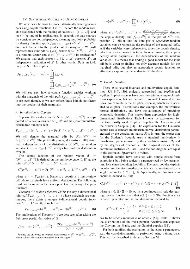
12
TABLE VINUMBER OF MEASUREMENTS AND ENERGY CONSUMPTION AT THE WIRELESS NODES FOR TWO DIFFERENT DATA RECOVERY QUALITY LEVELS. TWO
POLLUTANTS (CO, NO2) ARE MEASURED.
Medium Data Recovery Quality High Data Recovery QualityBaseline `1-`1 Proposed Baseline `1-`1 Proposed
Aggregated average relative error 1.4046 1.4230 1.3957 1.1148 1.1044 1.0969Total number of measurements 950 850 550 1400 1300 1050
EHWproc. (J) 4.84 × 10⁻⁶ 4.33 × 10⁻⁶ 2.80 × 10⁻⁶ 7.14 × 10⁻⁶ 6.63 × 10⁻⁶ 5.35 × 10⁻⁶
ESWproc. (J) 46.51 × 10⁻⁶ 41.62 × 10⁻⁶ 26.93 × 10⁻⁶ 68.54 × 10⁻⁶ 63.64 × 10⁻⁶ 51.41 × 10⁻⁶
ETx (J) 0.8586 0.7668 0.4968 1.2636 1.1718 0.9450Etotal (J) 0.8586 0.7668 0.4968 1.2636 1.1718 0.9450
component z(l) ∼ N (0, σzI) additive to the measurements,where σz is the noise standard deviation8 and I is the m(l) ×m(l) identity matrix. In this experiment, we vary the noise levelas σz ∈ {0, 2, 5} and calculate the aggregated average relativeerror as a function of the total number of measurements. Wefirst consider the case in which two pollutants are gatheredby each device. The considered schemes are (i) the proposedsystem with successive data recovery using the copula-basedalgorithm (the Student’s t copula is used); (ii) DCS [24],and; (iii) the baseline system [18], [27]. Figs. 9(a) and 9(b)show that the proposed system delivers superior performancecompared to the competing systems for moderate (σz = 2) andhigh (σz = 5) noise. Moreover, we observe that the proposedalgorithm is robust against noise, especially, when the numberof measurements is small. In particular, the aggregated averagerelative error increases on average 5.8% (σz = 2) and 18.7%(σz = 5) with respect to the noiseless case.
In case three pollutants are measured, the proposed systemsystematically outperforms the DCS scheme and the baselinesystem, under both moderate and high noise. Moreover, theproposed design continues to demonstrate robustness againstnoise, with the aggregated average relative error increasing onaverage only 4.2% (σz = 2) and 10.1% (σz = 5) comparedto the noiseless case. It is clear that the robustness of theproposed system increases with the number of pollutants.
C. Energy Consumption Analysis
We now study the impact of the proposed system onreducing the number of measurements and in turn the energyconsumption of the wireless nodes, for a given data recon-struction quality. The energy consumption at each node isbroken down into a sensing, processing and transmission part:Etotal = Esens. + Eproc. + ETx [63]. The sensing part, Esens.,depends on the amount of censored data; hence, its energyconsumption is the same for the proposed and the baselinesystem. We thus focus our comparison on the energy consump-tion due to the processing and transmission parts. Following atypical IoT design, we assume that the nodes are equipped withthe MSP430 micro-controller [64] and that communicationadheres to LoRa [58]. MSP430 architectures [64] are typicallybuilt around a 16-bit CPU running at 25 MHz, with a voltagesupply of V = 1.8 − 3.6 Volt and a current of I = 200
8We assume that the standard deviation of the noise is the same for allsources; hence, we drop the superscript (l).
μA/MIPS in the active mode. As discussed in Section III,every node generates a pseudorandom number, computes theproduct between this number and the censored value, addsit to the sum of the previous relayed values, and sendsthe final value to the next node. This operation is repeatedper measurement and source l ∈ {1, ..., `}. Neglecting thepseudorandom number generation part, the encoding operationboils down to a multiply-and-accumulate (MAC) operation.The MSP430 CPU cycles needed for a single signed 16-bit MAC operation are 17 for a hardware implementation orbetween 143 and 177 for a software implementation [64].Therefore, the time to perform a single MAC operation9 istHW = 17 cycles
25 MHz = 0.68 μs or tSW = 177 cycles25 MHz = 7.08 μs.
The total time to encode the measurements at each device canthen be calculated as t(•)
proc. =∑`
l=1 m(l) × t(•) and the totalprocessing energy as E(•)
proc. = V ∙ I ∙ t(•)proc., where (•) stands for
HW or SW. In order to calculate the energy consumption fortransmission, we used the LoRa energy consumption calculatorfrom Semtech [65], [66]. For a typical 12-byte payload packetwith a 14 dBm power level, a current at 44 mA and aspreading factor of 7, the transmission energy consumptionwas estimated at 5.4 mJ. In the scenario where two pollutants(CO and NO2) are encoded [and no noise is assumed in thecommunication medium], Table VI-B4 reports the number ofmeasurements and the energy consumption at the nodes for thebaseline system, the system using `1-`1 minimization [29], andthe proposed system. It is worth observing that the processingenergy is negligible compared to the energy consumed bythe transceiver. It is evident that for a comparable aggregatedaverage relative error the proposed system leads to a significantreduction in the number of transmitted measurements com-pared to the competition, which translates to critical energysavings at the nodes.
VII. CONCLUSION AND FUTURE WORK
We addressed the problem of data recovery from com-pressive measurements in large-scale WSN applications, suchas air-pollution monitoring. In order to efficiently capturestatistical dependencies among heterogeneous sensor data, weused copula functions [34], [35]. This enabled us to devisea novel CS-based reconstruction algorithm, built upon beliefpropagation [36], [67], which leverages multiple heteroge-neous signals (e.g., air pollutants) as side information in orderto improve reconstruction. Experiments using synthetic data
9We consider the higher value on the number of cycles for software.

13
and real sensor data from the USA EPA showed that theproposed scheme significantly improves the quality of datareconstruction with respect to prior state-of-the-art methods[23], [29], [68], even under sensing and communication noise.Furthermore, we showed that, for a given data reconstructionquality, the proposed scheme offers low encoding complexityand reduced radio transmissions compared to the state of theart, thereby leading to energy savings at the wireless devices.We conclude that our design effectively meets the demandsof a large-scale monitoring application. Future work shouldconcentrate on assessing the method on alternative datasets,such as the Intel-Berkeley Lab dataset [69], the dataset fromthe Center for Climatic Research [70], and the indoor datasetfrom the University of Padova [71].
REFERENCES
[1] E. Zimos, J. F. C. Mota, M. R. D. Rodrigues, and N. Deligiannis,“Bayesian compressed sensing with heterogeneous side information,”in IEEE Data Compression Conference, 2016.
[2] E. Zimos, J. F. Mota, M. R. Rodrigues, and N. Deligiannis, “Internet-of-things data aggregation using compressed sensing with side informa-tion,” in Int. Conf. Telecomm. (ICT). IEEE, 2016.
[3] I. F. Akyildiz and M. C. Vuran, Wireless sensor networks. John Wiley& Sons, 2010, vol. 4.
[4] C. Liu, K. Wu, and J. Pei, “An energy-efficient data collection frameworkfor wireless sensor networks by exploiting spatiotemporal correlation,”IEEE Trans. Parallel Distrib. Syst., vol. 18, no. 7, pp. 1010–1023, 2007.
[5] S. Yoon and C. Shahabi, “The clustered aggregation (CAG) techniqueleveraging spatial and temporal correlations in wireless sensor net-works,” ACM Trans. Sensor Net., vol. 3, no. 1, p. 3, 2007.
[6] H. Gupta, V. Navda, S. Das, and V. Chowdhary, “Efficient gathering ofcorrelated data in sensor networks,” ACM Trans. Sensor Net., vol. 4,no. 1, p. 4, 2008.
[7] M. Vecchio, R. Giaffreda, and F. Marcelloni, “Adaptive lossless entropycompressors for tiny IoT devices,” IEEE Trans. Wireless Commun.,vol. 13, no. 2, pp. 1088–1100, 2014.
[8] D. I. Sacaleanu, R. Stoian, D. M. Ofrim, and N. Deligiannis, “Compres-sion scheme for increasing the lifetime of wireless intelligent sensornetworks,” in European Signal Process. Conf. (EUSIPCO), 2012, pp.709–713.
[9] M. Crovella and E. Kolaczyk, “Graph wavelets for spatial traffic anal-ysis,” in Annu. Joint Conf. IEEE Comput. and Commun. (INFOCOM),vol. 3, 2003, pp. 1848–1857.
[10] A. Ciancio, S. Pattem, A. Ortega, and B. Krishnamachari, “Energy-efficient data representation and routing for wireless sensor networksbased on a distributed wavelet compression algorithm,” in Int. Conf.Inform. Process. Sensor Networks. ACM, 2006, pp. 309–316.
[11] J. Acimovic, B. Beferull-Lozano, and R. Cristescu, “Adaptive distributedalgorithms for power-efficient data gathering in sensor networks,” inInternational Conference on Wireless Networks, Communications andMobile Computing, vol. 2. IEEE, 2005, pp. 946–951.
[12] Z. Xiong, A. D. Liveris, and S. Cheng, “Distributed source coding forsensor networks,” IEEE Signal Process. Mag., vol. 21, no. 5, pp. 80–94,2004.
[13] V. Stankovic, A. D. Liveris, Z. Xiong, and C. N. Georghiades, “Oncode design for the slepian-wolf problem and lossless multiterminalnetworks,” IEEE Trans. Inf. Theory, vol. 52, no. 4, pp. 1495–1507, 2006.
[14] N. Deligiannis, E. Zimos, D. Ofrim, Y. Andreopoulos, and A. Munteanu,“Distributed joint source-channel coding with copula-function-basedcorrelation modeling for wireless sensors measuring temperature,” IEEESensor J., vol. 15, no. 8, pp. 4496–4507, 2015.
[15] F. Chen, M. Rutkowski, C. Fenner, R. C. Huck, S. Wang, and S. Cheng,“Compression of distributed correlated temperature data in sensor net-works,” in IEEE Data Compression Conf. (DCC), 2013, pp. 479–479.
[16] D. L. Donoho, “Compressed sensing,” IEEE Trans. Inf. Theory, vol. 52,pp. 1289–1306, 2006.
[17] E. J. Candes and M. B. Wakin, “An introduction to compressivesampling,” IEEE Signal Process. Mag., vol. 25, no. 2, pp. 21–30, 2008.
[18] J. Haupt, W. U. Bajwa, M. Rabbat, and R. Nowak, “Compressed sensingfor networked data,” IEEE Signal Process. Mag., vol. 25, no. 2, pp. 92–101, 2008.
[19] J. Tropp and A. C. Gilbert, “Signal recovery from random measurementsvia orthogonal matching pursuit,” IEEE Trans. Inf. Theory, vol. 53,no. 12, pp. 4655–4666, 2007.
[20] T. Blumensath and M. E. Davies, “Iterative hard thresholding for com-pressed sensing,” Applied Computational Harmonic Analysis, vol. 27,no. 3, pp. 265–274, 2009.
[21] D. Baron, S. Sarvotham, and R. G. Baraniuk, “Bayesian compressivesensing via belief propagation,” IEEE Trans. Signal Process., vol. 58,no. 1, pp. 269–280, 2010.
[22] D. L. Donoho, A. Maleki, and A. Montanari, “Message-passing algo-rithms for compressed sensing,” Proc. Nat. Academy Sci., vol. 106,no. 45, pp. 18 914–18 919, 2009.
[23] J. Haupt and R. Nowak, “Signal reconstruction from noisy randomprojections,” IEEE Trans. Inf. Theory, vol. 52, no. 9, pp. 4036–4048,2006.
[24] M. F. Duarte, S. Sarvotham, D. Baron, M. B. Wakin, and R. G. Baraniuk,“Distributed compressed sensing of jointly sparse signals,” in AsilomarConf. Signals, Syst., Comput., 2005, pp. 1537–1541.
[25] R. Masiero, G. Quer, D. Munaretto, M. Rossi, J. Widmer, and M. Zorzi,“Data acquisition through joint compressive sensing and principal com-ponent analysis,” in IEEE Global Telecommun. Conf. (GLOBECOM).IEEE, 2009, pp. 1–6.
[26] G. Quer, R. Masiero, G. Pillonetto, M. Rossi, and M. Zorzi, “Sensing,compression, and recovery for wsns: Sparse signal modeling and moni-toring framework,” IEEE Trans. Wireless Commun., vol. 11, no. 10, pp.3447–3461, 2012.
[27] C. Luo, F. Wu, J. Sun, and C. W. Chen, “Efficient measurementgeneration and pervasive sparsity for compressive data gathering,” IEEETrans. Wireless Commun., vol. 9, no. 12, pp. 3728–3738, 2010.
[28] S. Lee, S. Pattem, M. Sathiamoorthy, B. Krishnamachari, and A. Or-tega, “Spatially-localized compressed sensing and routing in multi-hopsensor networks,” in International Conference on GeoSensor Networks.Springer, 2009, pp. 11–20.
[29] J. F. C. Mota, N. Deligiannis, and M. R. D. Rodrigues, “Compressedsensing with prior information: Strategies, geometry, and bounds,” IEEETrans. Inf. Theory, vol. 63, no. 7, pp. 4472–4496, 2017.
[30] J. F. C. Mota, L. Weizman, N. Deligiannis, Y. Eldar, and M. R.Rodrigues, “Reference-based compressed sensing: A sample complexityapproach,” in IEEE Int. Conf. Acoust., Speech Signal Process. (ICASSP),2016.
[31] J. F. Mota, N. Deligiannis, and M. R. Rodrigues, “Compressed sens-ing with side information: Geometrical interpretation and performancebounds,” in IEEE Global Conf. Signal and Inform. Process. (GlobalSIP),2014, pp. 512–516.
[32] F. Renna, L. Wang, X. Yuan, J. Yang, G. Reeves, R. Calderbank,L. Carin, and M. R. Rodrigues, “Classification and reconstruction ofhigh-dimensional signals from low-dimensional features in the presenceof side information,” IEEE Trans. Inf. Theory, vol. 62, no. 11, pp. 6459–6492, 2016.
[33] Y. Liu, X. Zhu, and L. Zhang, “Noise-resilient distributed compressedvideo sensing using side-information-based belief propagation,” in IEEEInt. Conf. Network Infrastructure Digit. Content (IC-NIDC), 2012, pp.350–390.
[34] M. Sklar, Fonctions de repartition a n dimensions et leurs marges. Un.Paris 8, 1959.
[35] R. B. Nelsen, An Introduction to Copulas. Secaucus, NJ, USA:Springer-Verlag New York, Inc., 2006.
[36] D. J. MacKay, Information theory, inference and learning algorithms.Cambridge University Press, 2003.
[37] [Online]. Available: http://www3.epa.gov/airdata/.[38] D. L. Donoho and X. Huo, “Uncertainty principles and ideal atomic
decomposition,” IEEE Trans. Inf. Theory, vol. 47, no. 7, pp. 2845–2862,2001.
[39] E. J. Candes and T. Tao, “Decoding by linear programming,” IEEETrans. Inf. Theory, vol. 51, no. 12, pp. 4203–4215, 2005.
[40] V. Chandrasekaran, B. Recht, P. A. Parrilo, and A. S. Willsky, “Theconvex geometry of linear inverse problems,” Found. ComputationalMathematics, vol. 12, no. 6, pp. 805–849, 2012.
[41] J. F. C. Mota, N. Deligiannis, A. C. Sankaranarayanan, V. Cevher,and M. R. Rodrigues, “Dynamic sparse state estimation using `1 − `1minimization: Adaptive-rate measurement bounds, algorithms and appli-cations,” in IEEE Int. Conf. Acoust., Speech Signal Process. (ICASSP),2015.
[42] N. Vaswani and W. Lu, “Modified-CS: Modifying compressive sensingfor problems with partially known support,” IEEE Trans. Signal Pro-cess., vol. 58, no. 9, 2010.

14
[43] J. Scarlett, J. S. Evans, and S. Dey, “Compressed sensing with priorinformation: Information-theoretic limits and practical decoders,” IEEETrans. Signal Process., vol. 61, no. 2, pp. 427–439, 2013.
[44] M. A. Khajehnejad, W. Xu, A. S. Avestimehr, and B. Hassibi, “Weighted`1 minimization for sparse recovery with prior information,” in IEEEInt. Symp. Inf. Theory (ISIT), 2009, pp. 483–487.
[45] S. Oymak, M. A. Khajehnejad, and B. Hassibi, “Recovery threshold foroptimal weight `1 minimization,” in IEEE Int. Symp. Inf. Theory (ISIT),2012, pp. 2032–2036.
[46] M. Trocan, T. Maugey, J. E. Fowler, and B. Pesquet-Popescu, “Disparity-compensated compressed-sensing reconstruction for multiview images,”in IEEE Int. Conf. Multimedia and Expo (ICME), 2010, pp. 1225–1229.
[47] R. G. Gallager, “Low-density parity-check codes,” IRE Trans. on Inform.Theory, vol. 8, no. 1, pp. 21–28, 1962.
[48] C. Genest and L.-P. Rivest, “On the multivariate probability integraltransformation,” Stat. & Probability Lett., vol. 53, no. 4, pp. 391–399,2001.
[49] H. Joe, Multivariate models and multivariate dependence concepts.CRC Press, 1997, vol. 73.
[50] C. Genest and J. Mackay, “The joy of copulas: bivariate distributionswith uniform marginals,” Amer. Statistician, vol. 40, no. 4, pp. 280–283,1986.
[51] A. J. McNeil and J. Neslehova, “Multivariate archimedean copulas, d-monotone functions and -norm symmetric distributions,” Ann. Stat., pp.3059–3097, 2009.
[52] A. J. McNeil, R. Frey, and P. Embrechts, Quantitative risk management:concepts, techniques and tools. Princeton University Press, 2005.
[53] G. G. Roussas, An introduction to probability and statistical inference.Academic Press, 2003.
[54] S. Ji, Y. Xue, and L. Carin, “Bayesian compressive sensing,” IEEE Trans.Signal Process., vol. 56, no. 6, pp. 2346–2356, 2008.
[55] D. Zordan, G. Quer, M. Zorzi, and M. Rossi, “Modeling and generationof space-time correlated signals for sensor network fields,” in IEEEGlobal Telecommunications Conference (GLOBECOM), 2011, pp. 1–6.
[56] E. Y. Lam and J. W. Goodman, “A mathematical analysis of the DCTcoefficient distributions for images,” IEEE Trans. Image Process., vol. 9,no. 10, pp. 1661–1666, 2000.
[57] E. Bouye, V. Durrleman, A. Nikeghbali, G. Riboulet, and T. Roncalli,“Copulas for finance-a reading guide and some applications,” Available:http://ssrn.com/abstract=1032533, 2000.
[58] [Online]. Available: https://www.lora-alliance.org/.[59] F. J. Massey Jr, “The Kolmogorov-Smirnov test for goodness of fit,”
Amer. Statistical Assoc. J., vol. 46, no. 253, pp. 68–78, 1951.[60] C. Genest and L.-P. Rivest, “Statistical inference procedures for bivariate
Archimedean copulas,” Amer. Statistical Assoc. J., vol. 88, no. 423, pp.1034–1043, 1993.
[61] “Joao Mota,” https://github.com/joaofcmota/cs-with-prior-information/docs/docs.pdf.
[62] W. Breymann, A. Dias, and P. Embrechts, “Dependence structuresfor multivariate high-frequency data in finance,” Quantitative Finance,vol. 3, no. 1, pp. 1–14, 2003.
[63] O. Landsiedel, K. Wehrle, and S. Gotz, “Accurate prediction of powerconsumption in sensor networks,” in IEEE Workshop on EmbeddedNetworked Sensors (EmNetS). IEEE, 2005, pp. 37–44.
[64] T. Instruments, “The MSP430 hardware multiplier function and appli-cations,” Application Report, pp. 1–30, 1999.
[65] “Semtech LoRa Modem Design Guide,”www.semtech.com/images/datasheet/LoraLowEnergyDesign STD.pdf.
[66] “Semtech,” http://www.semtech.com/wireless-rf/rf-transceivers/sx1272.[67] R. G. Cowell, Probabilistic networks and expert systems: Exact compu-
tational methods for Bayesian networks. Springer Science & BusinessMedia, 2006.
[68] D. Baron, M. F. Duarte, S. Sarvotham, M. B. Wakin, and R. G. Baraniuk,“An information-theoretic approach to distributed compressed sensing,”in 45th Annu. Allerton Conf. Commun., Control, and Computing, 2005.
[69] P. Bodik, W. Hong, C. Guestrin, S. Madden, M. Paskin, andR. Thibaux. (2004, Feb.) Intel lab data. [Online]. Available:http://db.csail.mit.edu/labdata/labdata.html
[70] C. J. Willmott and K. Matsuura. (2009, Aug.) Global climate resourcepages. [Online]. Available: http://climate.geog.udel.edu/climate/
[71] R. Crepaldi, S. Friso, A. Harris, M. Mastrogiovanni, C. Petrioli,M. Rossi, A. Zanella, and M. Zorzi, “The design, deployment, andanalysis of signetlab: a sensor network testbed and interactive manage-ment tool,” in Int. Conf. Testbeds and Research Infrastructure for theDevelopment of Networks and Communities (TridentCom), 2007, pp.1–10.
Nikos Deligiannis (S’08, M’10) received theDiploma degree in electrical and computer engi-neering from the University of Patras, Greece, in2006, and the Ph.D. degree (Hons.) in applied sci-ences from Vrije Universiteit Brussel, Belgium, in2012. He is currently an Assistant Professor withthe Electronics and Informatics Department, VrijeUniversiteit Brussel.
From 2012 to 2013, he was a Post-DoctoralResearcher with the Department of Electronics andInformatics, Vrije Universiteit Brussel. From 2013
to 2015, he was a Senior Researcher with the Department of Electronic andElectrical Engineering, University College London, U.K., and also a TechnicalConsultant on Big Visual Data Technologies with the British Academy of Filmand Television Arts, U.K.
His current research interests include big data processing and analysis, ma-chine learning, Internet-of-Things networks, and distributed signal processing.He has authored over 80 journal and conference publications, book chapters,and two patent applications (one owned by iMinds, Belgium and the other byBAFTA, U.K.). He has received the 2011 ACM/IEEE International Conferenceon Distributed Smart Cameras Best Paper Award, the 2013 Scientific PrizeFWO-IBM Belgium, and the 2017 EURASIP Best Ph.D. Award.
Joao F. C. Mota received the M.Sc. degree andthe Ph.D. degree in Electrical and Computer En-gineering from the Technical University of Lisbon,Portugal, in 2008 and 2013, respectively. He alsoreceived the Ph.D. degree in Electrical and ComputerEngineering from Carnegie Mellon University, PA,USA, in 2013.
From 2013 to 2016, he was Senior ResearchAssociate at University College London, London,U.K. In 2017, he became Assistant Professor inthe School of Engineering and Physical Sciences
at Heriot-Watt University, Edinburgh, U.K., where he is also affiliated withthe Institute of Sensors, Signals, and Systems. His current research interestsinclude theoretical and practical aspects of high-dimensional data processing,inverse problems, optimization theory, machine learning, data science, anddistributed information processing and control. He was the recipient of the2015 IEEE Signal Processing Society Young Author Best Paper Award for thepaper “Distributed Basis Pursuit”, published in IEEE Transactions on SignalProcessing.
Evangelos Zimos received the Diploma in electricalengineering and computer science from Universityof Patras, Greece, in 2010. From Aug. 2010 to Dec.2012 he was working as communication engineer atthe Hellenic military and the industry. Since Feb.2013 he is a Ph.D. candidate in the Departmentof Electronics and Informatics, Vrije UniversiteitBrussel. Currently, he is with Motor Oil Hellas,Hellenic Refineries S.A., working as a senior elec-trical engineer on industrial automation, electricalequipment monitoring and protection.

15
Miguel R. D. Rodrigues (SM’15) received theLicenciatura degree in electrical and computer engi-neering from the University of Porto, Porto, Portu-gal, and the Ph.D. degree in electronic and electricalengineering from the University College London,U.K. He is currently a Reader in information theoryand processing with the Department of Electronicand Electrical Engineering, University College Lon-don, London, U.K. He was with the University ofPorto rising through the ranks from Assistant toAssociate Professor, where he was also the Head
of the Information Theory and Communications Research Group, Instituto deTelecomunicacoes Porto.
He has also held postdoctoral positions and visiting appointments withvarious institutions worldwide including University College London, Cam-bridge University, Princeton University, and Duke University from 2003 to2016. His research interests include the general areas of information theoryand processing with a current focus on sensing, analysis, and processing ofhigh-dimensional data. His work, which has led to more than 150 papers inthe leading international journals and conferences in the field, has also beenhonored with the Prestigious IEEE Communications and Information TheorySocieties Joint Paper Award 2011.
Dr. Rodrigues received fellowships from the Portuguese Foundation for Sci-ence and Technology and the Foundation Calouste Gulbenkian. Dr. Rodrigueshas served on the organizing and technical committees of various internationalconferences, including as Co-Chair of the Technical Programme Committee ofthe IEEE Information Theory Workshop 2016. He serves as Associate Editorto the IEEE Communications Letters and lead guest editor of the SpecialIssue on ”Information-Theoretic Methods in Data Acquisition, Analysis, andProcessing” of the IEEE Journal on Selected Topics in Signal Processing.He is also co-authoring a book on ”Information-Theoretic Methods in DataScience” to be published by Cambridge University Press.