Heuristic Algorithm for Coordinating Smart

Houses in MicroGrid.

Mohamed Arikiez 1, Floriana Grasso1, and Michele Zito 1

1Department of Computer Science, University of Liverpool, United

Kingdom

May 28, 2015

Abstract

This work presents a framework for e�ciently managing the energyneeds of a set of houses connected in a micro-grid con�guration. Themicro-grid consists of houses and local renewable plants, each seen asindependent agents with their speci�c goals. In particular houses have theoption to buy energy from the national grid or from the local renewableplants. We discuss a practical heuristic that leads to energy allocationschedules that are cost-e�ective for the individual houses and pro�tablefor the local plants. We present experiments describing the bene�ts of ourproposal. The results illustrate that houses and micro plants can makeconsiderable saving when they work in micro grid compared with workingalone.

1 Introduction

The world's energy needs are ever increasing [1, 2] and the investment in newpower plants is not going to cover the future demand [3]. The power sector

can be improved in many ways, using more renewable resources, or resorting tomore e�cient and environmentally friendly power plants. Also, Demand SideManagement and Demand Response could encourage consumers to modify theirenergy usage behaviour.

The concept of Smart Grid is relatively new. The Smart Grid is an en-hanced electrical grid in which information and communication technology isused to improve the power system and increase the pro�t of consumers, distrib-utors and generation companies. The key features of such infrastructure arereliability, �exibility, e�ciency, sustainability, peak curtailment, and demandresponse. The Smart Grid is also market enabling, it provides a platform foradvanced services, and increases the manageability of the available resources.To exploit the Smart Grid in residential buildings, we need new technologies

such as integrated communications, sensing and measurements, smart meters,advanced control, advanced components, power generation, and smart appli-ances [4]. Smart micro-grids [5] can be de�ned as a set of houses containingloads (appliances) and co-located resources (such as small PV arrays, or windplants) working as a single controllable system [6]. Smart micro-grids also o�erthe possibility to export the surplus of locally generated power to the nationalgrid.

There are plenty of studies that investigate methods for optimizing the cost ofelectricity in stand-alone residential buildings, based on electricity price, avail-ability of renewable power, or user preferences. These studies use di�erentalgorithms to achieve their goals. For example, studies [7�10] use algorithmsthat �nd the optimal cost of electricity, whereas [11�13] use heuristic methodswhich only guarantee suboptimal cost. Sharing local renewable power in smallcommunities is an active research area. Study [14], uses Mixed Integer LinearProgramming (MILP) to compare the cost of 20 houses working individually andthe same houses working in a micro-grid setup. Although this study adds someknowledge to the �eld, it does not tackle the important issue of computationtime. In studies of this type the time complexity of the particular algorithm in-creases with the system's granularity or the number of available appliances. Theauthors are only able to present examples that allocates resources over relativelylarge time slots. Furthermore, in this study each house uses only two appliances.Study [1] investigates the sharing of local renewable energy in a micro-grid. Agreedy energy search algorithm is used to match the predicted renewable powerwith the predicted house consumption. The proposed approach also minimizesthe power loss incurred while transferring electricity power along power lines bychoosing the nearest house to share renewable power with. Unfortunately theproposed algorithm does not scale well with the length of the time slots.

In this work, we investigate the e�ectiveness of a MILP-based strategy thatcan be used to solve a particular energy allocation problem within a given micro-grid. Our contribution is summarized in the following points:

� Design of a general micro-grid management system. Including fairly gen-eral notion of appliances.

� MILP applied to micro-grid control, with heuristic, for practical purposes.

� Preliminary empirical evaluation.

The rest of this paper is organized as follows: Section 2 details the systemde�nition and modeling of system entities, MILP formulation is presented insection 3, and the fourth section illustrates the results which are followed bydiscussions in Section 5. Finally, the paper ends with conclusions.

2 Allocation Problem

In this section we present the formalization of the computational problem dis-cussed in this paper.

(a) Conventional Grid (b) Smart MicroGrid with

LMGO

Fig. 1: Conventional grid vs smart MicroGrid

2.1 The micro-grid

A micro-grid consists of a set of houses H, and a set of micro-generation powerplants (or generators) R (see the example in Fig.(1)). Some houses (like H2, H3,or H4 in Fig.(1)) may be directly connected to a generator, and therefore theyare able to receive energy from it in a particularly e�cient way, but in general thehouses in the system may receive their power from any of the generators in themicro-grid or the National Electricity Grid (NEG). The energy exchange withina micro-Grid is controlled by a Local micro-Grid Optimizer (LMGO). The powerplants generate energy which can be either used by the houses in the micro-gridor exported to the NEG. Fig.(2) describes the possible energy exchanges betweena house, a generator and the NEG. Houses (and their appliances) can only useelectricity. The electricity comes in the house either from a generator (internalto the house or external) or from the grid. The labels on the arcs represent theunit cost that the entity at the end of the arrow will have to pay to the entityat the other end to get electricity from it. We assume that the energy producedby a generator r can be sent to a house h at a unit cost γr,h or exported tothe NEG at a cost ζr. Alternatively, a house can buy energy from the NEG ata cost λh. All costs might change over time (hence the dependence on a timeparameter t shown in the �gure).

2.2 Appliances

Each house h ∈ H is equipped with a set of appliances Ah = {A1, A2, . . . , Amh},

Appliances in a micro-grid are the main energy outlets. We assume that theappliances in the system can be easily switched on or o� without disrupting

Fig. 2: Diagram shows exchange local renewable power among micro-grid compo-nents.

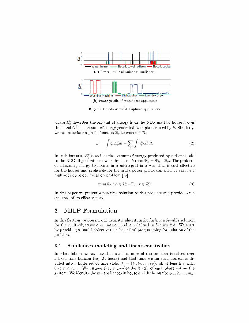
their functionalities. Washing machines, cookers, air-conditioning (AC) units,battery chargers are examples of suitable appliances whereas TV sets or Com-puters do not �t into such framework. Moreover we assume that the appliancesin a micro-grid can either be interruptible or uninterruptible, uniphase or mul-tiphase. Interruptible appliances are designed to be switched ON/OFF at anytime. Appliances of this type include heaters, cookers, or air-conditioning (AC)units. Uninterruptible appliances are not designed to be switched OFF once theyhave been switched ON until they �nish a particular task. Washing machinesare good examples of uninterruptible appliances. Heaters are also examples ofuniphase appliance. Any such appliance can either be OFF or ON and when itis ON it uses approximately a constant amount of power (nominal power). Notethat the restriction to the use of uniphase appliances is that only have a singleON state, without loss of generality, appliances that can run at one of severalpower levels can be simulated by a combination of several uniphase appliancesas de�ned in this paper. Multiphase appliances work in di�erent phases, eachusing a certain amount of power. A washing machine typically uses a lot ofenergy at the beginning of a wash cycle, to heat up the water, then uses littleenergy for some time, and a bit more again during the �nal spins. Fig.(3.(b))shows the typical power pro�le of three di�erent multiphase appliances. Withina given phase, multiphase appliances cannot be switched o�. We also assumethat some appliances may have constraints on how often they are run whileothers might be controlled by environmental factors such as the level of chargeof a battery, or particular desired values of room temperatures.

For the purpose of this study we assume that each appliance A operatesin ∆A > 0 (nominal) phases and for each appliance, it is possible to de�ne apower pro�le vector (α1, . . . , α∆A

) describing its energy needs. We assume thatτmin is length of the shortest phase. Each αj is a non-negative real number,corresponding to the average amount of power used by the appliance duringits jth phase. When switched on appliance A progresses through each of itsphases, starting from phase 1 up to phase ∆A at which point the appliance isswitched OFF. We also assume that for each appliance we know whether it isinterruptible or not, and the number of times it must be used, nA. Note thatsuch model �ts the di�erent types of appliances described before.

2.3 Optimization Problem

From the discussion so far it is evident that a micro-grid consists of distinctagents each with their own goals and priorities: houses need energy to run theirset of appliances according to pre-de�ned plans, generators produce energy thatcan be sold to the houses in the micro-grid or the NEG; houses want to purchasecheap energy whereas generators want to maximize their pro�t. In this settingwe can associate a cost function Ψh to each house h ∈ H:

Ψh =

∫λhL

hgdt+

∑r

∫γhrG

hrdt, (1)

(a) Power pro�le of uniphase appliances

(b) Power pro�le of multiphase appliances

Fig. 3: Uniphase vs Multiphase appliances

where Lhg describes the amount of energy from the NEG used by house h over

time, and Ghr the amount of energy generated from plant r used by h. Similarly,we can associate a pro�t function Ξr to each r ∈ R:

Ξr =

∫ζrE

rgdt+

∑h

∫γhrG

hrdt. (2)

In such formula, Erg describes the amount of energy produced by r that is soldto the NEG. If generator r owned by house h then Ψh = Ψh−Ξr. The problemof allocating energy to houses in a micro-grid in a way that is cost e�ectivefor the houses and pro�table for the grid's power plants can then be cast as amulti-objective optimization problem [15].

min(Ψh : h ∈ H;−Ξr : r ∈ R) (3)

In this paper we present a practical solution to this problem and provide someevidence of its e�ectiveness.

3 MILP Formulation

In this Section we present our heuristic algorithm for �nding a feasible solutionfor the multi-objective optimization problem de�ned in Section 2.3. We startby providing a (multi-objective) mathematical programming formulation of theproblem.

3.1 Appliances modeling and linear constraints

In what follows we assume that each instance of the problem is solved overa �xed time horizon (say 24 hours) and that time within such horizon is di-vided into a �nite set of time slots, T = {t1, t2, . . . , tT }, all of length τ with0 < τ < τmin. We assume that τ divides the length of each phase within thesystem. We identify themh appliances in house h with the numbers 1, 2, . . . ,mh.

Fig. 4: Multiphase appliance modeling

Without loss of generality, we also assume that each appliance i runs through∆hi (real) phases, of length τ . Note that real phases may be much shorter than

the nominal phases mentioned in Section 2.2. Thus we assume that real phasesare grouped into clutches corresponding to the nominal phases and the appli-ances are uninterruptible within each clutch (Fig.(4) shows an appliance withthree clutches). We use a dedicated binary variable xhi,j(t) for appliance i in(real) phase j. The variable holds the appliance ON/OFF state at time t.

Phi,j(t) = αhi,j · xhi,j(t) ∈{

0, . . . , αh∆hi

}. (4)

We also assume that appliance i in h can only be run between time slot th,isand th,if (with th,is ≤ th,if ), in a so called comfort interval speci�ed by the user,if needed. We model this using the following constraints

th,is −1∑t=0

xh,ij (t) +

tT∑t=th,i

f1 +1

xh,ij (t) = 0, (5)

where either sums may be empty if th,is = t1 or th,if = tT . If both equalitieshold (say if the user does not specify a comfort interval) the constraints vanish.

To enforce that appliance i in h runs nhi times in {th,is , . . . , th,if }, we need thefollowing constraints ∑

t∈{th,is ,...,th,i

f }

xh,ij (t) = nhi . (6)

Phases can be kept in order imposing∑t∈T

[t · xh,ij+1(t)− t · xh,ij (t)

]≥ 1. (7)

and to prevent interruption between any two consecutive phases, we use con-straint (7) with �=� replacing �≥�.

As mentioned before, the operation of some appliances depends on externalconditions rather than initial user demands. For instance charging a batterydepends on the battery charging state Θh

i (t) and its charging rate, αhi , whereasthe operations of an Air Conditioning (AC) unit depends on the room tem-

perature, Th,iin (t), the outside temperature and the device heating or coolingpower [8]. Appropriate constraints in such cases replace those in (6). In thecase of batteries, say, we need to use the following constraints.

Θhi (t) = Θh

i (t− 1) +1

4· π · Ph

i,1(t) ∀t : t ∈{th,is , . . . , th,if

}(8)

Θhi (th,is ) = βhi , Θh

i (th,if ) = βh

i (9)

where βhi is the initial state of charge of the battery, βh

i is the desired �nal stateof charge of the battery (usually full), and π is the battery charging e�ciency.In the case of heating/cooling units, the main task of the given unit is to keep

the room temperature within the comfort level [Th,imin, Th,imax] during bhi speci�ed

time intervals Ih1 , . . . , Ihbi. The relationship between room temperature and the

power allocated to the appliance is shown in Eq. (10).

Th,iin (t) = ε · Th,iin (t− 1) + (1− ε)[Tout(t)−

η

κPhi,1(t)

](10)

Th,imin ≤ Th,iin (t) ≤ Th,imax ∀t : t ∈ Ih1 ∪ . . . Ihbi

where ε is the appliance inertia, η is e�ciency of the system (with η > 0 for aheating appliance and η < 0 in the case of cooling), κ is the thermal conductivity,Tout(t) is outside temperature at time t.

3.2 Objective Function and Additional Constraints

For the purpose of our experiments we simplify the general model presented inSection 2.3. The cost function in Eq.(1) is replaced by the linear function

Ψh =∑t∈T

{λ(t)Lhg (t) +

∑r∈R

[γhr (t)Ghr (t)

]}∀h : h ∈ H, (11)

and similarly, the pro�t function in Eq.(2) is replaced by

Ξr =∑t∈T

{ζ(t)Erg(t) +

∑h∈H

[γhr (t)Ghr (t)

]}∀r : r ∈ R. (12)

Note that we are assuming that the cost of the energy from the NEG, λ, and thepro�t obtained selling energy to the grid, ζ, may vary over time but are otherwiseidentical for all houses and generators in the system. Also if r belongs to h thenγhr (t)= 0 ∀t, and Ψh is the right-hand side of (11) minus Ξr.

Few constraints need to be added to the system. There are the renewablepower constraints

Erg(t) +∑h∈H

Ghr (t) = Pr(t) ∀t : t ∈ T , ∀r : r ∈ R, (13)

where Pr(t) is the renewable power generated by r, and power balance equations,enforcing that the allocated power at any time slot, t, must equal power demandat that time

Lhg (t) +∑r∈R

Ghr (t) =∑i∈Ah

∆hi∑

j=0

Ph,ij (t), ∀t : t ∈ T , (14)

The key idea is to reduce the multi-objective problem to a single objectiveone using "modi�ed version" ε-constraint method [16] in order to treat all en-tities equally, and then use a MILP solver to �nd a feasible allocation. To thispurpose we consider the MILP obtained by using the constraints listed in 3.1along with the following objective function

Min

{ |H|∑i=1

Ψi −|R|∑i=1

Ξi

}(15)

and extra constraintsΨh ≤ Ψ̃h ∀h : h ∈ H (16)

Ξr ≥ Ξ̃r ∀r : r ∈ R (17)

where Ψ̃h, and Ξ̃r are the optimal costs of the energy allocation problem forhouse h and renewable plant r, considered as isolated units connected solely tothe NEG.

3.3 MILP-based Heuristic

Let MinCost denote the version of our problem restricted to a single house,with m uniphase appliances, to be allocated in one of two possible time slots.Also assume that the available renewable power is always 1

2

∑mi=1 αi, and the

NEG electricity price is λ > 0. A straightforward reduction from the Partitionproblem [17] shows thatMinCost is NP-hard. Therefore there is little hope thatthe MILP de�ned in the previous section might be solved quickly if the numberof appliances is large. In our experiments we resort to an MILP-based heuristicalgorithm to get a feasible solution in acceptable time. The basic idea is to usean o�-the-shelf LP-solver to generate a feasible solution but without runningthe optimization process to completion. The LP-solver uses dual relaxation to�nd a lower bound on the optimum and stops as soon as the di�erence betweenthe cost of the best feasible solution so far and the lower bound on the optimumbecomes smaller than a prede�ned threshold. Also, we can put time limit ordeadline to stop the algorithm.

4 Empirical Evaluation

All the experiments in this work have been done on a PC with an Intel(R)core(TM) i7-2600 CPU @ 3.4 GHZ, RAM is 16 GB, 64-bit Operating System(windows 7). In addition, Gurobi [18] has been used to solve LP and MILPproblems, whereas the Java was the main tools to build our model. Three casestudies will be demonstrated to illustrate the advantages and disadvantages ofour approach.

4.1 First case study

The main goals of this case study is to show the e�ect of renewable powerdemand on saving or pro�t.

4.1.1 Input setting

20 houses with variant renewable power generation capacities, see Table (1), andthree independent renewable plants (PV array with maximum generation capac-ity = 5KW/H, two wind turbines, with 5KW/H, 10KW/H generation capacity,respectively) will be used to investigate the performance of our algorithm. Thepower pro�les of uninterruptible appliances are shown in Table.(2), whereas theinterruptible appliances are given in Table (3).

In addition, τ = 5 minutes, T=288 time slots, ζ = 4.5 P/KWH, ξ = 0.0P/KWH, γ(t) = 8.5 P/KWH, π = 0.8. Regarding AC's parameters, ε = 0.96,η= 30 KW/ ◦C, κ = 0.98, Tmin= 18.0 ◦C, Tmax=22.0

◦C. Fig.(5) shows solarand wind power generated in Liverpool, UK (53°24´N 2°59´W), using 3.5KW/HPV array and 2KW/H wind turbine. These data will be approximated andscaled up/down to model variant set of PV arrays and wind turbines.

(a) Solar power for three days

in April, May, and June 2012

(b) Wind power for three days in

January, March, and June

Fig. 5: Renewable Power, for di�erent three days in April, May and June 2012 inLiverpool

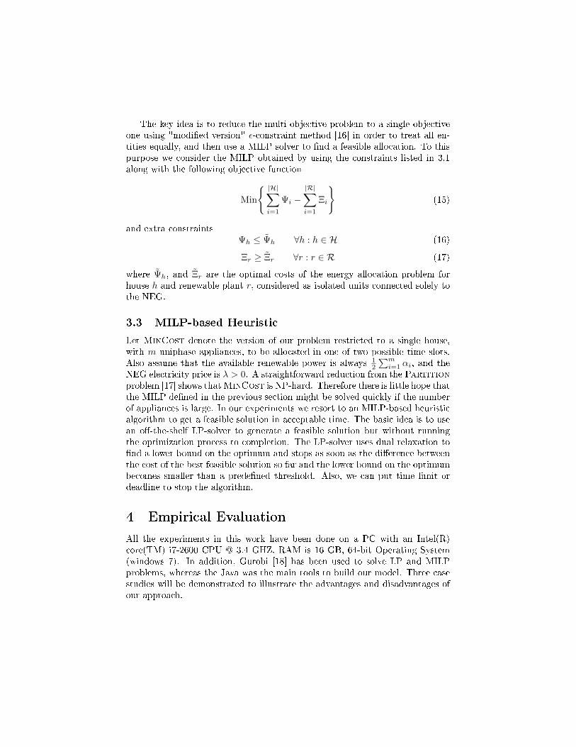
The electricity prices are shown in Fig.(6). In the �rst case study, dynamicpricing 1 will be used, whereas the rest will be used in the second and third casestudies.

Table 1: PV array generation capacity of houses

House No 5,10,15 1,6,11,16,19 2,7,12,17,20 3,8,13,18 4,9,14

Capacity 0.0 KW 1.0 KW 1.5 KW 2.0 KW 2.5 KW

Fig. 6: Electricity Price, one �xed pricing scheme and two di�erent dynamic pricingschemes.

Fig.(7) illustrates the outside temperature. Comfortable time for each ap-pliance in each house is shown in Table(4). Three scenarios will be used in thiscase study to examine the e�ect of electricity demand on saving. These scenar-ios are low demand, medium demand, and high demand, See Table(5,6, and 7).

Fig. 7: Outside Temperature

4.1.2 Findings

Fig.(8a) displays the average pro�t of three scenarios, low demand, mediumdemand, and high demand. The houses with high demand, in general, canmake more pro�t because the relationship between saving and renewable powerconsumption is positive. In contrast, Fig(8b) shows the relative MILP Gap ofthe three scenarios. As we can see, MILP Gap of high demand scenario is stillabove 100% after 30 minutes of running time that means the solution foundcould be far from optimality (we can save more by giving algorithm more time),it could be so close to optimality though. In addition, the �rst and secondscenarios are so close to optimality because MILP gap is less than 1 %.

Table 2: Multiphase uninterruptible appliances

Laundry Dryer α in KW 3.2 0.28 0 3.2 0.28φ in minutes 15 10 5 20 10

Dishwasher α in KW 0.2 2.7 0.2 2.7 0.2φ in minutes 5 15 15 20 5

Washing Machine α in KW 2.2 0.28 2.2 0.28 -φ in minutes 10 20 10 20 -

(a) Average pro�t in microgrid (b) the relative MILP Gap

Fig. 8: The result of low demand, medium demand, and high demand scenarios for20 houses and 3 renewable independent plants

Fig. (9) depicts pro�t stability in low and high demand scenarios. Therelationship between run time and average pro�t of all entities is positive, butit does not always hold for each entity. For instance, House No.17 in Fig.(9b)made more pro�t after 1, 5, and 10 minutes of calculation time than after15 minutes but in general the average pro�t increases with time until it reachoptimality. Fig.(10) illustrates the pro�t made by each component in micro-grid

(a) Low demand (b) High demand

Fig. 9: Pro�t stability in micro grid of �rst and third scenarios.

in three scenarios. Note that the �rst �fe house in medium demand scenarios,surprisingly, made more pro�t than the �rst �fe houses in high demand scenariobecause in medium demand scenario, the �rst �fe houses has 6 to 7 applianceswhereas the reset in around 4 and 5 houses so they consume a lot of localrenewable power for cheap price, we have not put details about exact numberof appliance and its details in each house for each scenarios due to page limit.Also, this behavior is expected in MILP heuristic algorithm because the solutionis not optimal.

Table 3: Interruptible appliances

Interruptible appliances α Depend on

Water heater 3.1 KW/t -

Electric Towel Radiator 1.5 KW/t -

Electric cooker 2.5 KW/t -

Plug-in Hybrid Electric Vehicle 0.35 KW /t Θ(ts)=2.0, Θ(tf )=16.0

Air conditioner 2.3 KW/t Tmin=18, Tmax=22

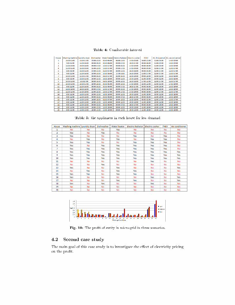
Table 4: Comfortable Interval

Table 5: the appliances in each house for low demand

Fig. 10: The pro�t of entity in micro-grid in three scenarios.

4.2 Second case study

The main goal of this case study is to investigate the e�ect of electricity pricingon the pro�t.

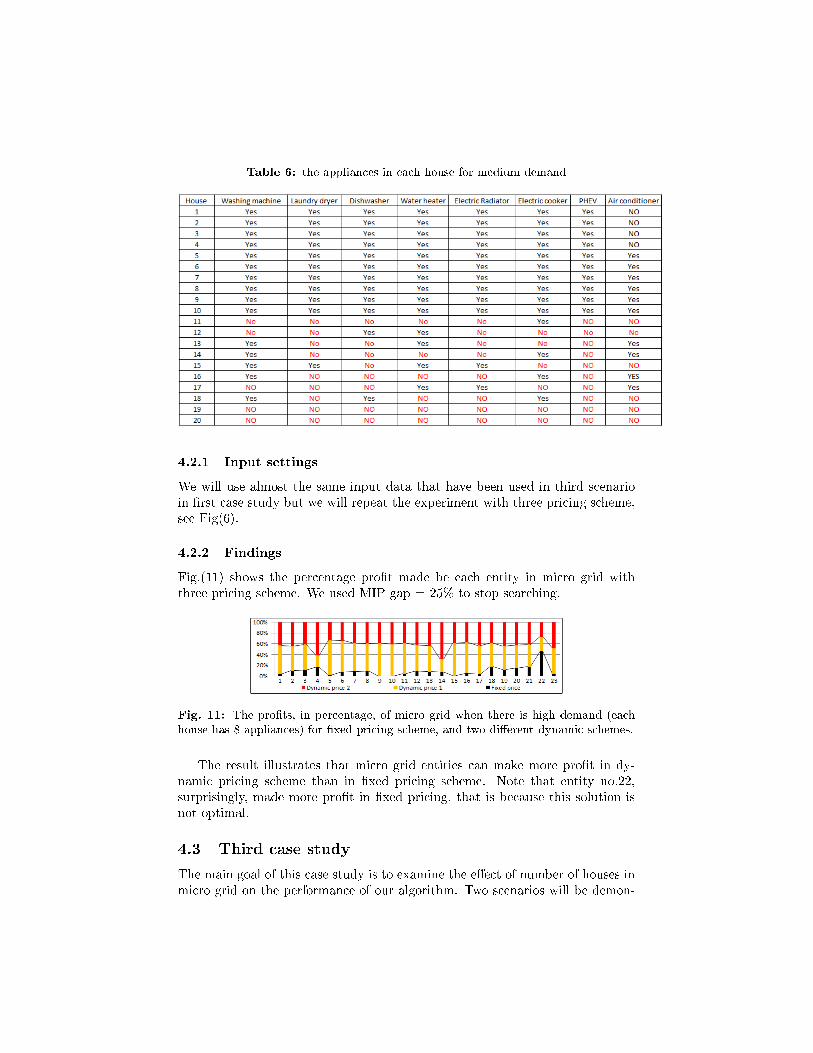
Table 6: the appliances in each house for medium demand

4.2.1 Input settings

We will use almost the same input data that have been used in third scenarioin �rst case study but we will repeat the experiment with three pricing scheme,see Fig(6).

4.2.2 Findings

Fig.(11) shows the percentage pro�t made be each entity in micro grid withthree pricing scheme. We used MIP gap = 25% to stop searching.

Fig. 11: The pro�ts, in percentage, of micro grid when there is high demand (eachhouse has 8 appliances) for �xed pricing scheme, and two di�erent dynamic schemes.

The result illustrates that micro grid entities can make more pro�t in dy-namic pricing scheme than in �xed pricing scheme. Note that entity no.22,surprisingly, made more pro�t in �xed pricing, that is because this solution isnot optimal.

4.3 Third case study

The main goal of this case study is to examine the e�ect of number of houses inmicro grid on the performance of our algorithm. Two scenarios will be demon-

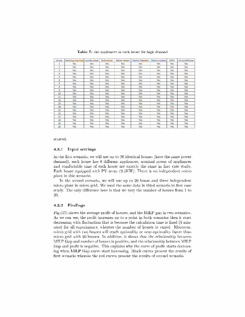
Table 7: the appliances in each house for high demand

strated.

4.3.1 Input settings

In the �rst scenario, we will use up to 20 identical houses (have the same powerdemand), each house has 8 di�erent appliances, nominal power of appliancesand comfortable time of each house are exactly the same in �rst case study.Each house equipped with PV array (2.5KW). There is no independent microplant in this scenario.

In the second scenario, we will use up to 20 house and three independentmicro plant in micro grid. We used the same data in third scenario in �rst casestudy. The only di�erence here is that we vary the number of houses from 1 to20.

4.3.2 Findings

Fig.(12) shows the average pro�t of houses, and the MILP gap in two scenarios.As we can see, the pro�t increases up to a point in both scenarios then it startdecreasing with �uctuation that is because the calculation time is �xed (5 min-utes) for all experiments, whereas the number of houses is varied. Moreover,micro grid with two houses will reach optimality or near-optimality faster thanmicro grid with 20 houses. In addition, it shows that the relationship betweenMILP Gap and number of houses is positive, and the relationship between MILPGap and pro�t is negative. This explains why the curve of pro�t starts decreas-ing when MILP Gap curve start increasing. Black curves present the results of�rst scenario whereas the red curves present the results of second scenario.

Fig. 12: Average cost and MILP Gap of houses in two scenarios

5 Discussion and conclusion

5.1 Fairness issues

By converting the problem from multi objectives to single objective one, fairnessissue could raise. Constraints (16) and (17) are needed to reduce unfairnessissue. Fig.(10) shows the individual pro�t of each entity. As we can see, houseno. 5, 10, and 15, which are the houses that does not have PV array, madepro�t higher than house no. 9 (equipped with PV array). The main reason forthis fairness issue is that this solution is suboptimal. Further work is needed tocope with this issue.

5.2 Pro�t stability

The stability of the pro�t depends on size of the problem (number of inte-ger variables) and MILP Gap, if problem is small, the algorithm will reachoptimality/near-optimality relatively fast and the pro�t will be almost stable,and vice versa. See Fig.(8) and Fig.(9).

Fig.(8b) shows, after 30 minutes of run time, the MILP gap still around100%, which means that the optimal solution may be still far on optimality, itcould be so close, though.

5.3 Scalability

Increasing the number of entities in micro-grid does not always increase thepro�ts of these entities. Fig.(12) shows that the relationship between the numberof houses and pro�t is not always positive. As we can see in both scenarios, thepro�t has positive relationship with the number of houses up to a point, afterthat the relationship become negative, that is because we increase the number ofhouses whereas run time is �xed. Future work, this study provided preliminaryinvestigation. Therefore, more investigation is needed to improve the fairnessof the algorithm. Also, we can improve the e�ciency of the micro-grid byprioritizing entities of micro grid.

To conclude, this work illustrates how an appropriate using MILP Heuristiccan be for solving huge optimization problem, the results shows that the sub-

optimal cost of each house in micro grid is cheaper than the optimal cost of eachhouse working alone.

References

[1] Zhichuan Huang, Ting Zhu, Yu Gu, David Irwin, Aditya Mishra, andPrashant Shenoy. Minimizing electricity costs by sharing energy in sustain-able microgrids. In Proceedings of the 1st ACM Conference on EmbeddedSystems for Energy-E�cient Buildings, pages 120�129. ACM, 2014.

[2] Anastasios I Dounis and Christos Caraiscos. Advanced control systemsengineering for energy and comfort management in a building environmenta review. Renewable and Sustainable Energy Reviews, 13(6):1246�1261,2009.

[3] Aldo Vieira Da Rosa. Fundamentals of renewable energy processes. Aca-demic Press, 2012.

[4] Saima Aman, Yogesh Simmhan, and Viktor K Prasanna. Energy man-agement systems: state of the art and emerging trends. CommunicationsMagazine, IEEE, 51(1):114�119, 2013.

[5] Sunetra Chowdhury and Peter Crossley. Microgrids and active distributionnetworks. The Institution of Engineering and Technology, 2009.

[6] R.H. Lasseter. Microgrids. In Power Engineering Society Winter Meeting,2002. IEEE, volume 1, pages 305�308 vol.1, 2002.

[7] Zhi Chen, Lei Wu, and Yong Fu. Real time price based demand responsemanagement for residential appliances via stochastic optimization and ro-bust optimization. IEEE TRANSACTIONS ON SMART GRID, 2012.

[8] Tanguy Hubert and Santiago Grijalva. Modeling for residential electricityoptimization in dynamic pricing environments. IEEE TRANSACTIONSON SMART GRID, 2012.

[9] KM Tsui and SC Chan. Demand response optimization for smart homescheduling under real-time pricing. IEEE TRANSACTIONS ON SMARTGRID, 2012.

[10] A Barbato and G Carpentieri. Model and algorithms for the real time man-agement of residential electricity demand. In Energy Conference and Ex-hibition (ENERGYCON), 2012 IEEE International, pages 701�706. IEEE,2012.

[11] E Matallanas, M Castillo-Cagigal, A Gutiérrez, F Monasterio-Huelin,E Caamaño-Martín, D Masa, and J Jiménez-Leube. Neural network con-troller for active demand-side management with pv energy in the residentialsector. Applied Energy, 91(1):90�97, 2012.

[12] Federica Mangiatordi, Emiliano Pallotti, Paolo Del Vecchio, and Fabio Lec-cese. Power consumption scheduling for residential buildings. In 201211th International Conference on Environment and Electrical Engineering(EEEIC), pages 926�930. IEEE, 2012.

[13] Thillainathan Logenthiran, Dipti Srinivasan, and Tan Zong Shun. Demandside management in smart grid using heuristic optimization. IEEE Trans-actions on Smart Grid, 3(3):1244�1252, 2012.

[14] Matthias Huber, Florian Sanger, and Thomas Hamacher. Coordinatingsmart homes in microgrids: A quanti�cation of bene�ts. In 2013 4thIEEE/PES Innovative Smart Grid Technologies Europe (ISGT EUROPE),pages 1�5. IEEE, 2013.

[15] Pawel Malysz, Shahin Sirouspour, and Ali Emadi. Milp-based rolling hori-zon control for microgrids with battery storage. In Industrial ElectronicsSociety, IECON 2013-39th Annual Conference of the IEEE, pages 2099�2104. IEEE, 2013.

[16] George Mavrotas. E�ective implementation of the ε-constraint method inmulti-objective mathematical programming problems. Applied Mathemat-ics and Computation, 213(2):455�465, 2009.

[17] Alessandro Agnetis, Gianluca de Pascale, Paolo Detti, and Antonio Vicino.Load scheduling for household energy consumption optimization. IEEETransactions on Smart Grid, 4(4):2364�2373, 2013.

[18] Inc. Gurobi Optimization. Gurobi optimizer reference manual, 2015.