HEURISTIC ALGORITHM FOR SINGLE RESOURCE CONSTRAINED PROJECT SCHEDULING PROBLEM … · 2009-12-11 · We consider the problem of resource distribution at the point of minimization

Yugoslav Journal of Operations Research Volume 19 (2009) Number 2, 281-298 DOI:10.2298/YUJOR0902281S

HEURISTIC ALGORITHM FOR SINGLE RESOURCE CONSTRAINED PROJECT SCHEDULING PROBLEM BASED

ON THE DYNAMIC PROGRAMMING

Ivan STANIMIROVIĆ1, Marko PETKOVIĆ2 Predrag STANIMIROVIĆ3* and Miroslav ĆIRIĆ4

1,2,3,4University of Niš, Department of Mathematics and informatics, Faculty of Sciences and Mathematics,

[email protected], [email protected], [email protected], [email protected]

Received: May 2006 / Accepted: October 2009

Abstract: We introduce a heuristic method for the single resource constrained project scheduling problem, based on the dynamic programming solution of the knapsack problem. This method schedules projects with one type of resources, in the non-preemptive case: once started an activity is not interrupted and runs to completion. We compare the implementation of this method with well-known heuristic scheduling method, called Minimum Slack First (known also as Gray-Kidd algorithm), as well as with Microsoft Project. Keywords: Resource scheduling, dynamic programming, knapsack problem, DELPHI.

1. INTRODUCTION

In practice most organizations work within limited resources, so projects are subject to the same constraint. A new project may seek an additional use of resources, so it is needed to ensure that they really would be available.

* Corresponding author

I. Stanimirović, M. Petković, P. Stanimirović, M. Ćirić / Heuristic algorithm 282

On the other hand, the time constraints are always present, so project manager must work under that boundary.

Resource leveling is a way to resolve having too much work assigned to resources, known as resource over allocation.

The network diagram can be used to find opportunities for shortening the project schedule. This involves looking at where we can cut the amount of time it takes to complete activities on the critical path, for example, by increasing the resources available to these activities. Another solution is to identify where any other routes might have some slack. We may then be able to reallocate resources to reduce the pressure on the team members who are responsible for activities on the critical path.

We consider the problem of resource distribution at the point of minimization of the project makespan, and introduce a heuristic method for solving the single resource constrained project scheduling problem, based on the knapsack problem and dynamic programming. The total number of available resource units is constant and specified in advance. A unit of resource cannot be shared by two or more activities. An activity is ready to be processed only when all its predecessor activities are completed and the number of resource units required by it are free and can be allocated to it. Once started, an activity is not interrupted and runs to completion.

When leveling resources, we do not change resource assignments, nor task informa-tion. We only delay tasks.

In a dynamic programming solution to the knapsack problem, we calculate the best combination for all knapsack sizes up to M [12]: for j:=1 to N do for i:=1 to M do if i-size[j]>=O then if cost[i]<(cost[i-size[j]]+val[j]) then begin cost[i]:=cost[i-size[j]]+val[j];

best[i]:=j end;

In this program, N is the number of items, val[j] is the value of jth item, size[j] is its volume, cost[i] is the highest value that can be achieved with a knapsack of capacity i and best[i] is the last item that was added to achieve that maximum (this is used to recover the contents of the knapsack). First, we calculate the best that we can do for all knapsack sizes when only items of type A (for j = 1) are taken, then we calculate the best that we can do when only A’s and B’s (for j = 2) are taken, etc. The solution reduces to a simple calculation for cost[i]. Suppose an item j is chosen for the knapsack: then the best value that could be achieved for the total would be val[j] + cost[i - size[j]], where cost[i - size[j]] is the optimal filling of the rest of the knapsack. If this value exceeds the best value that can be achieved without an item j, then we update cost[i] and best[i]; otherwise we leave them alone. A simple induction proof shows that this strategy solves the problem [12].


In this paper we propose a new strategy to solve the single resource constrained project scheduling problem. In each stage of the scheduling we consider a schedule time t and the corresponding eligible set of activities which could be started at the moment t without violation of given constraints which define the project. As it is proposed in [14] and [9], we activate a subset of activities from the eligible set solving the knapsack problem maximizing the resource utilization. But, instead of Greedy randomized adaptive search procedure (GRASP), used in [9], we apply the dynamic programming and Bellman’s principle (see [1]).

The paper is organized as follows. In the second section we state mathematical formulation of the problem and compare the project duration computed by our algorithm with the early finish of the project.

In the third section the algorithm and several implementation details are described. In the last section we compare the implementation of our algorithm with known

software Microsoft Project 2003® and Gray-Kidd algorithm. 2. MATHEMATICAL FORMULATION OF THE PROBLEM

A project consists of a set of activities J = {Ai}i∈I, partially ordered by precedence constraints, where I = {1,…,n} is a set of activities indices and n is a number of activities required by the project. It is assumed that the project requires only one type of resources. The entire project is defined as the ordered pair (J, R), where the natural number R denotes the resource maximal units available in the project. Each of activities Ai is defined as the ordered triple

Ai = (pi,, ri, Pi), i ∈ I,

where pi ∈ N represents the processing time (duration) of activity Ai, value ri∈N is a number of resources needed for Ai, and iP I⊂ is an array which contains predecessors indices for Ai. An activity Ai is said to be a predecessor of Aj, when Aj cannot start until Ai has finished. This fact is written as i∈Pj or Ai < Aj, where ’<’ defines the precedence relationship. Similarly Aj is said to be a successor activity of Ai. We assume that the number ri is fixed for the lasting time of activity Ai.

Let F denotes the set including all pairs of activities with predecessor and successor relationships. These pairs define a digraph of the project G = (J, F), where (Ai, Aj) ∈ F if and only if i∈ Pj, Ai, Aj ∈ J.

A project starts at time t = 0. A schedule for the project is an assignment of a start time s

it to each activity Ai. An activity is said to be scheduled when it is assigned a start time. The vector defining starts of activities included into the project (J, R) is defined as the ordered n-tuple 1( ,..., )s s s

nt t t= of natural numbers, and it is called start vector of the project. Similarly denote the vector of activities finishes by 1( ,..., )f f f

nt t t= . The finish of each activity


is computed from its start as f s

i i it t p= + . Vectors ts and tf are being calculated in our algorithm.

A feasible schedule is a schedule that satisfies the given precedence and resource constraints. An optimum schedule is a feasible schedule that optimizes the given objective function. Our goal is to find start time s

it for each activity Ai due to minimize the project completion time (makespan) of the project, calculated by : max{ | }.f

iDur t i I= ∈ We define the resource units required by Ai in the scheduling time t as follows:

, ,

0,

s ft ti i i

i i ir t t t

r x rotherwise

⎧ ≤ ≤⎪= =⎨⎪⎩

where 1tix = when the activity Ai is started and still not finished (in the time interval

s fi it t t≤ ≤ ), and 0t

ix = otherwise. Formally, the aim of the general single resource constrained project scheduling

problem is to find an optimal schedule, and can be formulated by the following mathematical model, in the time t:

min max{ | }fiDur t i I= ∈ (2.1)

. .( )( ) s fj j is t j I i P t t∀ ∈ ∀ ∈ ≥ (2.2)

( ) ti

i I

t r R∈

∀ ∈ ≤∑N (2.3)

Our objective is to minimize the makespan of the project. Each activity needs to be started after all its predecessors activities finish (condition (2.2)), and in every moment t, the total number of occupied resources is less than R (condition (2.3)). Proposition 2.1. Condition (2.2) can be written in the following equivalent form:

( )( ) f fj j i jj I i P t t p∀ ∈ ∀ ∈ − ≥ (2.4)

Observe that the condition (2.4) is equivalent with the corresponding one from [15]. Therefore, mathematical model (2.1)-(2.3) is equivalent with corresponding one,

described in [9], [15], in the case when one type of resources is used. Schedule ts of the project (J, R) is feasible if conditions (2.2) and (2.3) are satisfied.

A feasible schedule is optimal if (2.1) is fulfilled. Next lemma can be easily proven by the induction. This lemma gives a stopping

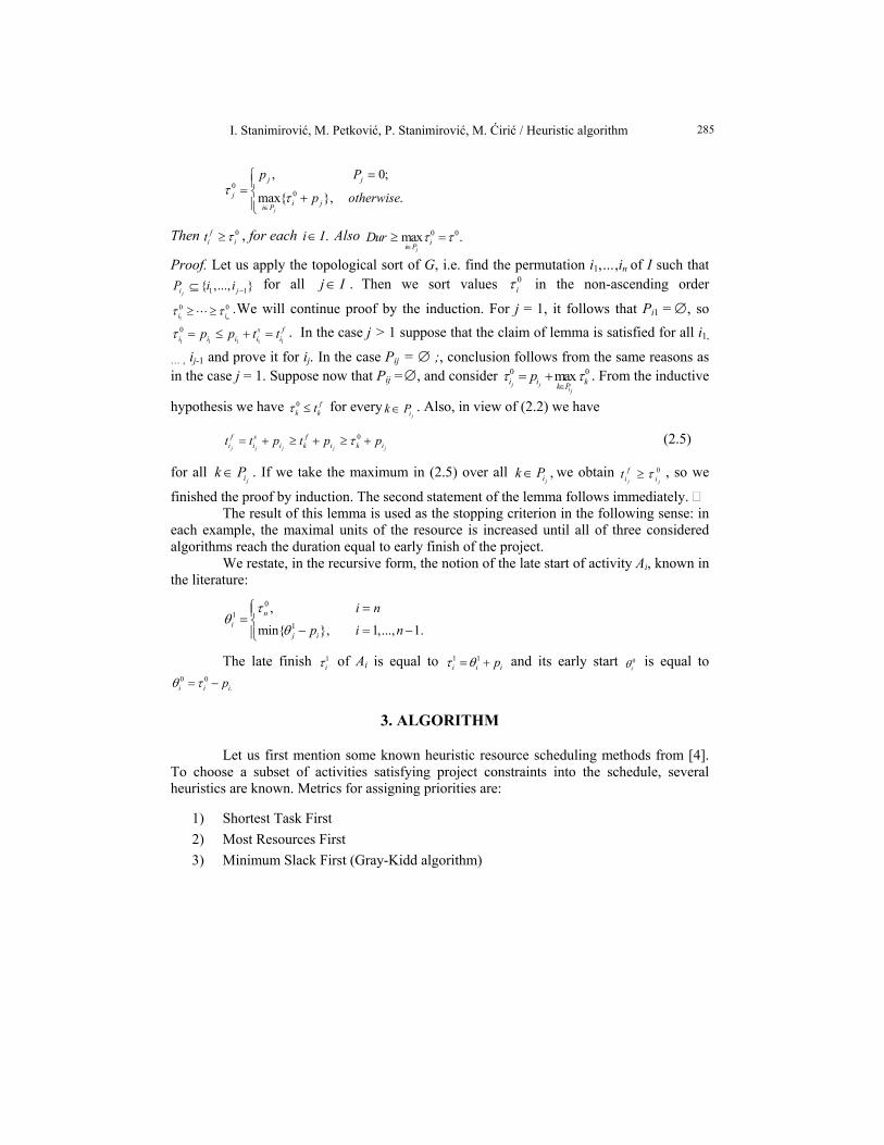
criterion for increasing maximal unit’s availability of the resource, i.e. the early finish of the project. Lemma 2.1 Let ts be the feasible schedule of the project (J, R). Let us consider the early finish 0

jτ for each activity Aj, j ∈ I, recursively as follows:


00

, 0;

max{ }, .j

j j

ji ji P

p P

p otherwiseτ τ∈

=⎧⎪= ⎨ +⎪⎩

Then 0f

i it τ≥ , for each .i I∈ Also 0 0max .j

ii PDur τ τ

∈≥ =

Proof. Let us apply the topological sort of G, i.e. find the permutation i1,…,in of I such that 1 1{ ,..., }

ji jP i i −⊆ for all j I∈ . Then we sort values 0iτ in the non-ascending order

1

0 0ni iτ τ≥ ≥ .We will continue proof by the induction. For j = 1, it follows that Pi1 = ∅, so

1 1 1 1 1

0 s fi i i i ip p t tτ = ≤ + = . In the case j > 1 suppose that the claim of lemma is satisfied for all i1,

… , ij-1 and prove it for ij. In the case Pij = ∅ ;, conclusion follows from the same reasons as in the case j = 1. Suppose now that Pij = ∅, and consider 0 0max

j ji j

i i kk Ppτ τ

∈= + . From the inductive

hypothesis we have 0 fk ktτ ≤ for every

jik P∈ . Also, in view of (2.2) we have

0j j j j j

f s fi i i k i k it t p t p pτ= + ≥ + ≥ + (2.5)

for all jik P∈ . If we take the maximum in (2.5) over all ,

jik P∈ we obtain 0

j j

fi it τ≥ , so we

finished the proof by induction. The second statement of the lemma follows immediately. The result of this lemma is used as the stopping criterion in the following sense: in

each example, the maximal units of the resource is increased until all of three considered algorithms reach the duration equal to early finish of the project.

We restate, in the recursive form, the notion of the late start of activity Ai, known in the literature:

01

1

,

min{ }, 1,..., 1.n

ij i

i n

p i n

τθ

θ

⎧ =⎪= ⎨− = −⎪⎩

The late finish 1iτ of Ai is equal to 1 1

i i ipτ θ= + and its early start 0iθ is equal to

0 0.i i ipθ τ= −

3. ALGORITHM

Let us first mention some known heuristic resource scheduling methods from [4]. To choose a subset of activities satisfying project constraints into the schedule, several heuristics are known. Metrics for assigning priorities are:

1) Shortest Task First 2) Most Resources First 3) Minimum Slack First (Gray-Kidd algorithm)


4) Most Critical Followers 5) Most Successors

There are many papers comparing alternative heuristic algorithms. Patterson and

Davis in [6], [7] compared these heuristics, in serial and parallel modes and achieved the result the most effective algorithm is Minimum Slack First. The similar results are achieved in [10]. The Minimum Slack First method is described in [5] (p. 225–233).

Kochetov and Stolyar [9] devise an evolutionary algorithm which com-bines genetic algorithm, path relinking, and tabu search. In order to select a subset of activities from the eligible set into the schedule, they solve the knapsack problem. The idea of using the knapsack problem with objective function maximizing the re-source utilization ratio is introduced in [13] and [14]. In order to solve the knapsack problem stated for the sake of resource utilization, in [9] and [14] use GRASP (greedy randomized adaptive search procedure) algorithm from [8]. GRASP is an iterative multi-start algorithm. There are two phases in every iteration: a greedy adaptive randomized construction phase and a local search phase. Starting from the feasible solution built during the greedy adaptive randomized construction phase, the local search explores its neighborhood until a local optimum is found. The best solution found overall the different iterations is kept as the result [8]. A solution x is said to be in the basin of attraction of the global optimum if local search starting from x leads to the global optimum. Once the neighborhood and objective function are determined, different starting solutions can be used to start the local search in a multi-start procedure. If the starting solution is in the basin of attraction of the global optimum, local search finds the global optimum. Otherwise, a non-global local optimum is found [11]. Using greedy solutions as starting points for local search in a multi-start procedure will usually lead to good, though, most often, suboptimal solutions. This is because the amount of variability in greedy solutions is small and it is less likely that a greedy starting solution will be in the basin of attraction of a global optimum. If there are no ties in the greedy function values or, if a deterministic rule is used to break ties, there is no variability and a multistart procedure would produce the same solution in each iteration [11].

In this section we will introduce an algorithm for resource scheduling, called DynamicRes, which is based on the knapsack problem and the dynamic programming. This heuristic gives better results with respect to Gray-Kidd algorithm in most cases. Algorithm DynamicRes is being written in the programming language DELPHI.

The algorithm requires a sequence of activities, and the following parameters for each activity ,iA i I∈ :

- duration of the activity (integer pi), - array of ordinal numbers of its predecessors, denoted by Pi, - units of resource required (integer ri).

Also, the input parameter of the algorithm is total number of resource units available in the project, denoted by R.


Output of algorithm are beginnings of activities after the resource scheduling is performed, i.e. the start vector 1( ,..., )s s

nt t of the project activities as well as the corresponding makespan of the project.

We use the status of each activity, denoted with Stati:

0, ,1, .

ii

i

A is not startedStat

A is finished⎧

= ⎨⎩

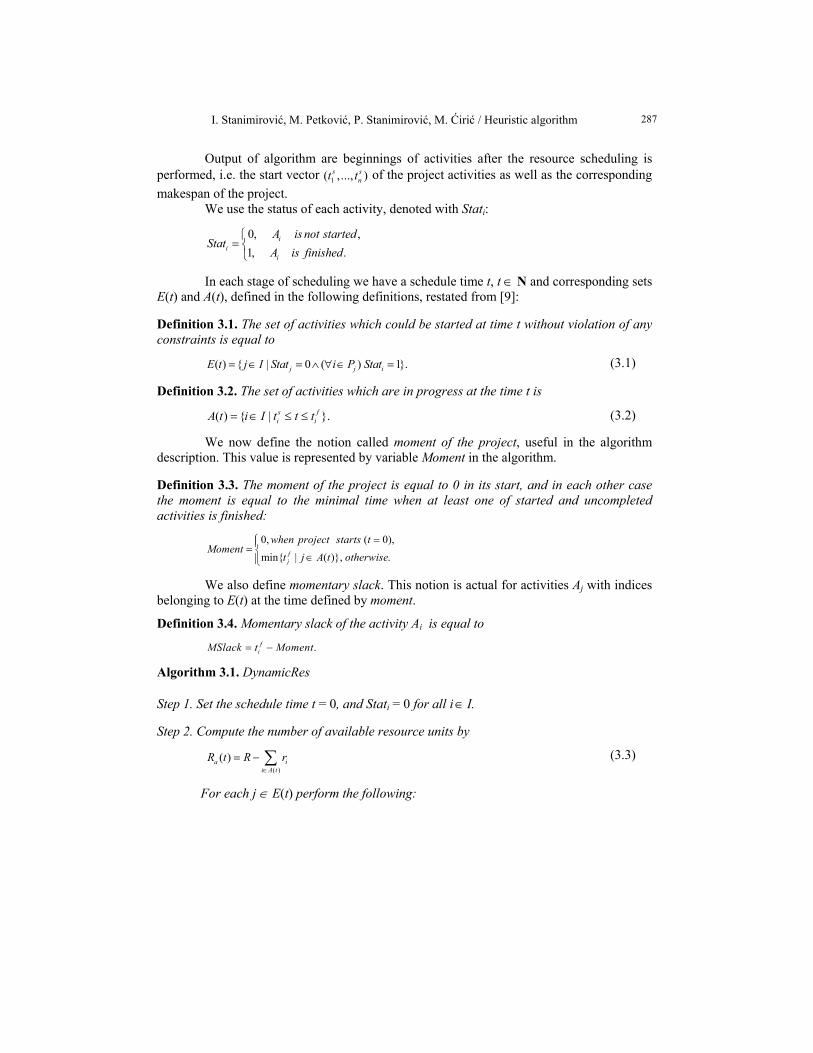
In each stage of scheduling we have a schedule time t, t ∈ N and corresponding sets E(t) and A(t), defined in the following definitions, restated from [9]:

Definition 3.1. The set of activities which could be started at time t without violation of any constraints is equal to

( ) { | 0 ( ) 1}.j j iE t j I Stat i P Stat= ∈ = ∧ ∀ ∈ = (3.1)

Definition 3.2. The set of activities which are in progress at the time t is

( ) { | }.s fi iA t i I t t t= ∈ ≤ ≤ (3.2)

We now define the notion called moment of the project, useful in the algorithm description. This value is represented by variable Moment in the algorithm. Definition 3.3. The moment of the project is equal to 0 in its start, and in each other case the moment is equal to the minimal time when at least one of started and uncompleted activities is finished:

0, ( 0),min{ | ( )}, .f

j

when project starts tMoment

t j A t otherwise=⎧⎪= ⎨ ∈⎪⎩

We also define momentary slack. This notion is actual for activities Aj with indices belonging to E(t) at the time defined by moment.

Definition 3.4. Momentary slack of the activity Ai is equal to

.fiMSlack t Moment= −

Algorithm 3.1. DynamicRes Step 1. Set the schedule time t = 0, and Stati = 0 for all i ∈ I. Step 2. Compute the number of available resource units by

( )

( )a ii A t

R t R r∈

= − ∑ (3.3)

For each j ∈ E(t) perform the following:


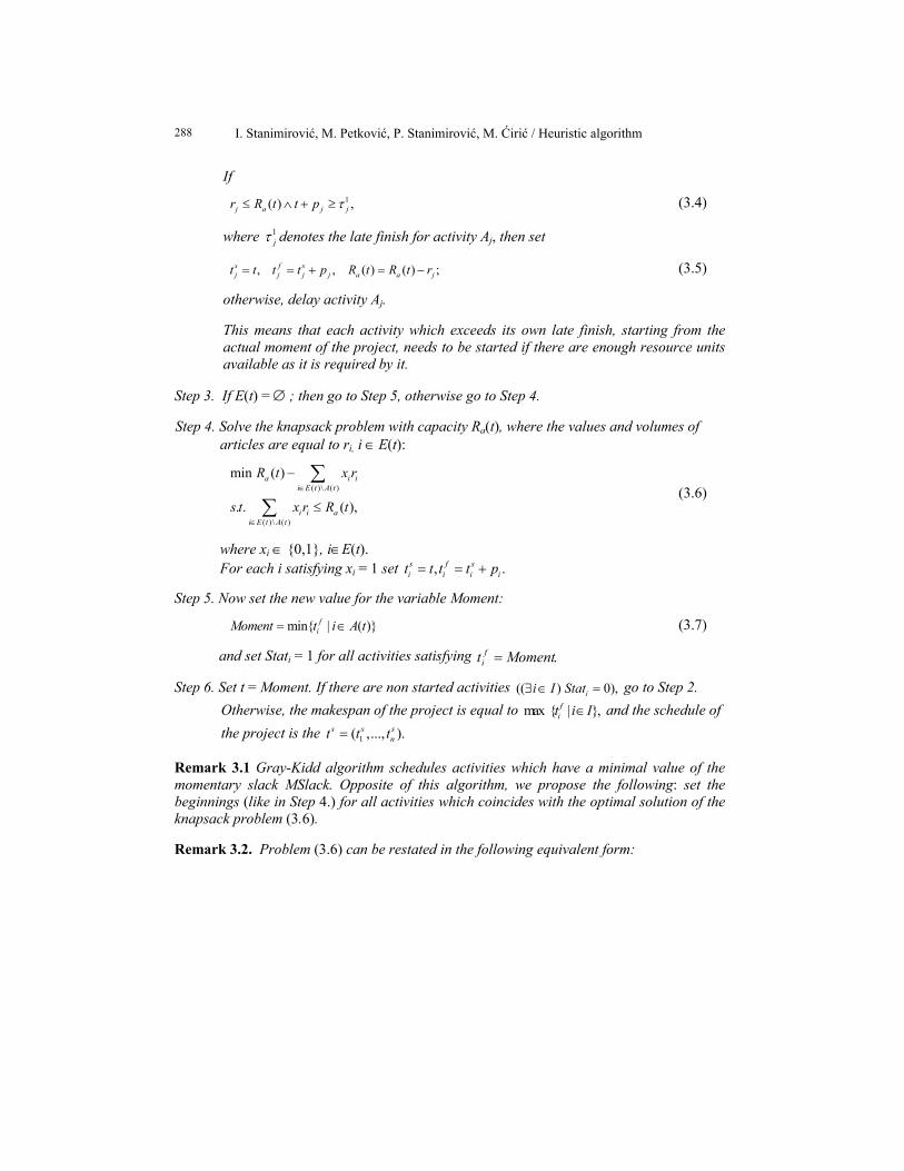
If 1( ) ,j a j jr R t t p τ≤ ∧ + ≥ (3.4)

where 1jτ denotes the late finish for activity Aj, then set

, , ( ) ( ) ;s f sj j j j a a jt t t t p R t R t r= = + = − (3.5)

otherwise, delay activity Aj. This means that each activity which exceeds its own late finish, starting from the actual moment of the project, needs to be started if there are enough resource units available as it is required by it.

Step 3. If E(t) = ∅ ; then go to Step 5, otherwise go to Step 4. Step 4. Solve the knapsack problem with capacity Ra(t), where the values and volumes of

articles are equal to ri, i ∈ E(t):

( )\ ( )

( ) \ ( )

min ( )

. . ( ),

a i ii E t A t

i i ai E t A t

R t x r

s t x r R t∈

∈

−

≤

∑

∑ (3.6)

where xi ∈ {0,1}, i∈E(t). For each i satisfying xi = 1 set , .s f s

i i i it t t t p= = +

Step 5. Now set the new value for the variable Moment:

min{ | ( )}fiMoment t i A t= ∈ (3.7)

and set Stati = 1 for all activities satisfying .Momentt fi =

Step 6. Set t = Moment. If there are non started activities (( ) 0),ii I Stat∃ ∈ = go to Step 2. Otherwise, the makespan of the project is equal to max { | },f

it i I∈ and the schedule of the project is the 1( ,..., ).s s s

nt t t=

Remark 3.1 Gray-Kidd algorithm schedules activities which have a minimal value of the momentary slack MSlack. Opposite of this algorithm, we propose the following: set the beginnings (like in Step 4.) for all activities which coincides with the optimal solution of the knapsack problem (3.6). Remark 3.2. Problem (3.6) can be restated in the following equivalent form:


( )\ ( )

( ) \ ( )

max

. . ( ),

i ii E t A t

i i ai E t A t

x r

s t x r R t∈

∈

≤

∑

∑ (3.8)

Problem (3.8) is a one-dimensional variant of the knapsack problem stated in [9] and [14], and a variant of the classical 0-1 knapsack problem (see, for example [2]). In order to solve (3.8), instead of the GRASP algorithm used in [9] and [14], we use the dynamic programming. Therefore, we speak of items representing requirements of the resource. The set of weights (volumes) as well as the set of values is equal to {ri | i∈I}. To avoid trivial cases we assume

ii I

r R∈

≥∑ and ,ir R≤ for each i∈ I. Comparing problem (3.8)

with the dynamic programming solution of the knapsack problem, restated from [12], the following analogies are evident:

- the objective function cost is equivalent with( )\ ( )

i ii E t A t

x r∈∑ ;

- the knapsack size M is equivalent with the number of available resource units, denoted by Ra(t), which is defined in (3.3) and (3.5);

- number N of different types of items is replaced by the cardinal number of the set I, denoted by n;

- val[j] = size[j] = rj; - Assignment best[i] = j implies xj = 1 in (3.6) and (3.8).

It is known that the knapsack problem exhibits optimal substructure, and its optimal solution contains within optimal solution to sub problems [3]. Typically, the total number of distinct sub problems is a polynomial in the input size. When a recursive algorithm revisits the same problem over and over again, we say that the optimization problem has overlapping sub problems. Dynamic programming algorithms typically take advantage of overlapping sub problems by solving each sub problem once and then storing the solution in a table [3]. Also, it is known that greedy algorithms do not always yield optimal solutions [3]. Remark 3.3 Using the main idea of the Gray-Kidd algorithm, in the case when we have more solutions for the knapsack problem, we use the solution containing activity with the minimal value for MSlack.

Here we consider an example to discuss about the difference between the Gray-Kidd algorithm and DynamicRes algorithm. Example 3.1 Durations, units of the resource required and predecessors of all activities in the project are arranged in the following table.


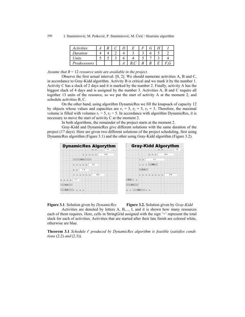
Activities A B C D E F G H I Duration 4 4 2 4 3 3 6 5 2 Units 5 5 3 6 4 5 7 3 4 Predecessors A B,C B B E F,G

Assume that R = 12 resource units are available in the project.

Observe the first actual interval: [0, 2]. We should numerate activities A, B and C, in accordance to Gray-Kidd algorithm. Activity B is critical and we mark it by the number 1. Activity C has a slack of 2 days and it is marked by the number 2. Finally, activity A has the biggest slack of 4 days and is assigned by the number 3. Activities A, B and C require all together 13 units of the resource, so we put the start of activity A at the moment 2, and schedule activities B, C.

On the other hand, using algorithm DynamicRes we fill the knapsack of capacity 12 by objects whose values and capacities are r1 = 5, r2 = 5, r3 = 3. Therefore, the maximal volume is filled with volumes r1 = 5, r2 = 5. In accordance with algorithm DynamicRes, it is necessary to move the start of activity C at the moment 2.

In both algorithms, the remainder of the project starts at the moment 2. Gray-Kidd and DynamicRes give different solutions with the same duration of the

project (17 days). Here are given two different solutions of the project scheduling, first using DynamicRes algorithm (Figure 3.1) and the other using Gray-Kidd algorithm (Figure 3.2).

Figure 3.1. Solution given by DynamicRes Figure 3.2. Solution given by Gray-Kidd

Activities are denoted by letters A, B,..., I, and it is shown how many resources each of them requires. Here, cells in StringGrid assigned with the sign ’>’ represent the total slack for each of activities. Activities that are started after their late finish are colored white, otherwise are blue. Theorem 3.1 Schedule ts produced by DynamicRes algorithm is feasible (satisfies condi-tions (2.2) and (2.3)).


Proof. Start time tsj for each activity Aj can be determined in two different ways, applying

Step 2 and Applying Step 4. Firstly we verify Condition (2.2). Using Step 2 in a fixed schedule time t we

schedule all activities whose indices satisfy j ∈ E(t) and (3.4) and set tsj = t for these activiti-

es. On the other hand, from Step 5, it is satisfied max{ | 1}.fi iMoment t Stat≥ = After setting t

= Moment in Step 6 it is satisfied max{ | 1}.fi it t Stat≥ = From (3.5) we conclude that

max{ | 1}s fj i it t t Stat= ≥ = , for each j∈E(t) satisfying (3.4). Therefore, we conclude

( ) .s fj j ii P t t∀ ∈ ≥

In the second case, according to Step 4 of DynamicRes algorithm, we conclude that in the knapsack problem are included only these activities Aj satisfying j ∈ E(t)\A(t). Therefore, in accordance with (3.1), all predecessors included in the knapsack are finished (( ) 1)j ii P Stat∀ ∈ = . Moreover, in Step 4 we schedule activities corresponding to the optimal solution of the knapsack problem. Analogous to the previous case, according to Step 5, condition (2.2) is satisfied for all activities included.

We now verify condition (2.3). It is clear that condition (2.3) can be written as

( )

( ) ii A t

t N r R∈

∀ ∈ ≤∑ (3.9)

In view of (3.3), this condition is later equivalent with

( ) ( ) 0.at N R t∀ ∈ ≥ (3.10)

Now, Step 2 satisfies condition (3.10) because of (3.5) and condition (3.4).

In the sequel we prove that Step 4 also satisfies (3.10). Denote by A’(t) the set of indices of just started activities:

'( ) { | }.siA t i I t t= ∈ =

Since tsi = t implies i ∈A’(t), we conclude

( ) ( ) '( )A t A t A t= ∪

after Step 4. At this moment, the number of available resources is

'( )( ) ( )a a i

i A t

R t R t r∈

= − ∑ (3.11)

According to condition in the knapsack problem (3.6), we conclude Ra(t) ≥ 0. Taking into account (3.3), we get

( ) '( )( ) 0a i i

i A t i A tR t R r r

∈ ∈

= − − ≥∑ ∑ (3.12)

Denote by A’’(t) the set of just finished activities in Step 6:


''( ) { | }.fiA t i I t Moment= ∈ =

Now, in Step 2 it is satisfied ( ) ( ) '( ) \ ''( )A t A t A t A t= ∪ and applying (3.12) we obtain

( ) '( ) ''( ) ( ) '( )( ) 0.a i i i i i

i A t i A t i A t i A t i A tR t R r r r R r r

∈ ∈ ∈ ∈ ∈

= − − + ≥ − − ≥∑ ∑ ∑ ∑ ∑

The proof is complete.

4. NUMERICAL EXPERIMENTS

In this section we compare three algorithms for resources scheduling: algorithm included in MS Project, Gray-Kidd algorithm and DynamicRes algorithm. According to our assumptions of the algorithm, in MS Project it is assumed that resources leveling cannot split task and check box Level only within available slack in Resource Leveling options is cleared.

Example 4.1. Consider the project defined as follows:

Activities A B C D E F G H Duration 5 4 4 9 5 5 4 4 Units 4 5 2 6 2 3 7 8 Predecessors A B C A G

Increasing the number of available resource units we get the following table. The

early finish for this example is 14 days, so we stop searching for new solutions when all three algorithms reach this limit, using the result of lemma 2.1.

Duration of the project

Max. units Ms Project Gray-Kidd DynamicRes 8 26 26 26 9 25 25 22

10 22 22 22 11 22 22 22 12 22 22 22 13 22 18 18 14 18 17 18 15 18 17 18 16 18 17 14 17 18 17 14 18 14 14 14

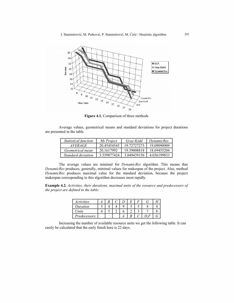
Data presented in the table are illustrated by the following chart:


Figure 4.1. Comparison of three methods

Average values, geometrical means and standard deviations for project durations are presented in the table.

Statistical function Ms Project Gray-Kidd DynamicRes

AVERAGE 20.45454545 19.72727273 19.09090909 Geometrical mean 20.1617992 19.39008818 18.69455204 Standard deviation 3.559877424 3.849439156 4.036199833

The average values are minimal for DynamicRes algorithm. This means that

DynamicRes produces, generally, minimal values for makespan of the project. Also, method DynamicRes produces maximal value for the standard deviation, because the project makespan corresponding to this algorithm decreases most rapidly. Example 4.2. Activities, their durations, maximal units of the resource and predecessors of the project are defined in the table:

Activities A B C D E F G HDuration 5 4 4 9 5 5 4 4 Units 4 5 2 6 2 3 7 8 Predecessors A B C D,F G

Increasing the number of available resource units we get the following table. It can easily be calculated that the early finish here is 22 days.


Duration of the project Max. units Ms Project Gray-Kidd DynamicRes

8 26 26 31 9 27 27 22

10 26 26 22 11 22 22 22

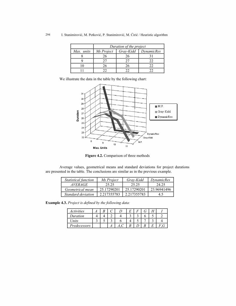
We illustrate the data in the table by the following chart:


Average values, geometrical means and standard deviations for project durations are presented in the table. The conclusions are similar as in the previous example.

Statistical function Ms Project Gray-Kidd DynamicRes AVERAGE 25.25 25.25 24.25

Geometrical mean 25.17290201 25.17290201 23.96941496 Standard deviation 2.217355783 2.217355783 4.5

Example 4.3. Project is defined by the following data:

Activities A B C D E F G H I Duration 4 4 2 4 3 3 6 5 2 Units 3 5 3 6 4 5 7 3 4 Predecessors A A,C B D B E F,G


Increasing the number of available units of the resource, we get the following table. The early finish for this example is 15 days.


7 31 29 29 8 24 22 24 9 22 22 22

10 21 21 19 11 21 21 19 12 20 18 19 13 18 18 18 14 16 16 16 15 16 16 16 16 16 16 16 17 15 15 15

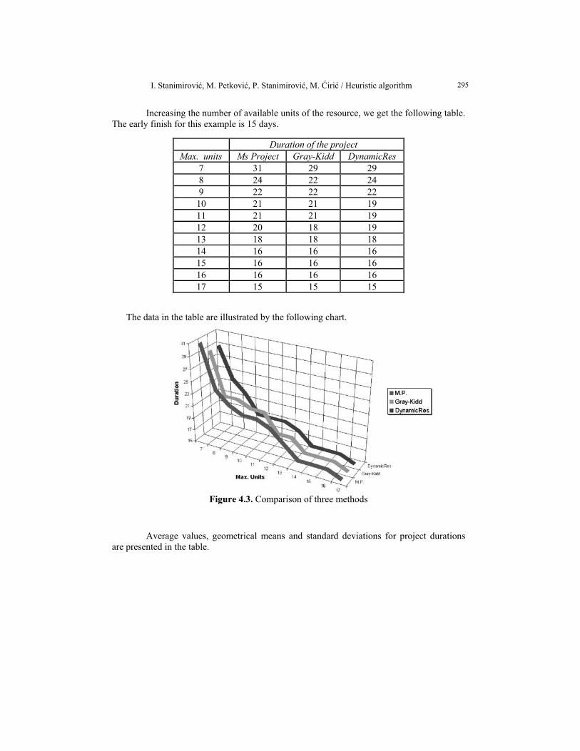
The data in the table are illustrated by the following chart.


Average values, geometrical means and standard deviations for project durations

are presented in the table.



AVERAGE 20 19.45454545 19.36363636 Geometrical mean 19.55234723 19.097246 18.99493701 Standard deviation 4.69041576 4.107642544 4.201731245

In this case, the maximal standard deviation produces the Ms Project. But, this fact

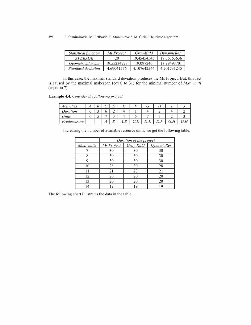
is caused by the maximal makespan (equal to 31) for the minimal number of Max. units (equal to 7). Example 4.4. Consider the following project:

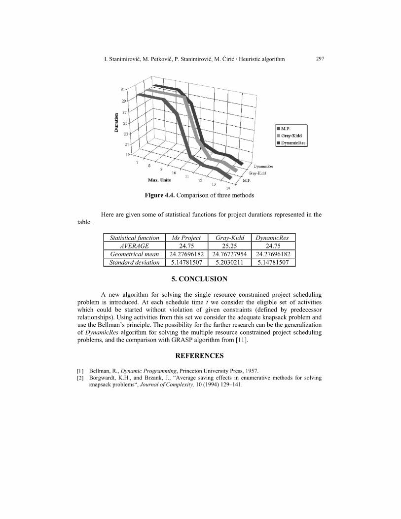
Activities A B C D E F G H I J Duration 6 3 6 2 4 1 4 2 4 2 Units 6 5 7 3 4 5 7 3 2 3 Predecessors A B A,B C,E D,E D,F G,H G,H

Increasing the number of available resource units, we get the following table.


7 30 30 30 8 30 30 30 9 30 30 30

10 28 30 28 11 21 23 21 12 20 20 20 13 20 20 20 14 19 19 19

The following chart illustrates the data in the table.



Here are given some of statistical functions for project durations represented in the table.


AVERAGE 24.75 25.25 24.75 Geometrical mean 24.27696182 24.76727954 24.27696182 Standard deviation 5.14781507 5.2030211 5.14781507

5. CONCLUSION

A new algorithm for solving the single resource constrained project scheduling problem is introduced. At each schedule time t we consider the eligible set of activities which could be started without violation of given constraints (defined by predecessor relationships). Using activities from this set we consider the adequate knapsack problem and use the Bellman’s principle. The possibility for the farther research can be the generalization of DynamicRes algorithm for solving the multiple resource constrained project scheduling problems, and the comparison with GRASP algorithm from [11].

REFERENCES

[1] Bellman, R., Dynamic Programming, Princeton University Press, 1957. [2] Borgwardt, K.H., and Brzank, J., “Average saving effects in enumerative methods for solving

кnapsack problems“, Journal of Complexity, 10 (1994) 129–141.


[3] Cormen, T. H., Leiserson, C. E., and Rivest, R. L., Introduction to Algorithms, MIT Press & McGraw-Hill, 1990.

[4] Osgood, N., Simulation and Resource Simulation and Resource- Based Scheduling, Presentation, 2004.

[5] Petrić, J., Operations Research, Savremena Administracija, Beograd, 1983. (In Serbian) [6] Patterson, J.H., “A comparison of exact approaches for solving the multiple constrained resource

project scheduling problem“, Management Science, 30 (7) (1984) 854-867. [7] Davies, E.M., “An experimental investigation of resource allocation in multiactivity projects”,

Operational Research Quarterly, 24 (11) (1976) 1186-1194. [8] Feo, T., and Resende, M.G.C., “Greedy randomized adaptive search procedures”, Journal of

Global Optimization, 6 (1995) 109–134. [9] Kochetov, Y., and Stolyar, A., “Evolutionary local search with variable neighborhood for the

resource constrained project scheduling problem“, in: Proceedings of the 3rd International Workshop of Computer Science and Information Technologies, Russia, 2003.

[10] Lawrence, S.R., “A computational comparison of heuristic scheduling techniques”, Technical Report, Graduate School of Industrial Administration, Carnegie-Mellon University, 1985.

[11] Pitsoulis, L.S., and Resende, M.G.C., “Greedy randomized adaptive search procedures“, AT&T Labs Research Technical Report, January 18, 2001.

[12] Sedgewick, R., Algorithms, Addison-Wesley publishing company, Massachusetts, Menlo Park, California, London, Amsterdam, Don Mills, Ontario, Sydney, 1984.

[13] Valls, V., Balletin, F., and Quintanilla, S., “A population-based approach to the resource-constrained project scheduling problem”, Technical report 10-2001, University of Valencia, 2001.

[14] Valls, V., Balletin, F., and Quintanilla, S., “A population-based approach to the resource-constrained project scheduling problem”, Annals of Operations Research, 131 (2004) 305-324.

[15] Verma, S., “An optimal breadth-first algorithm for the preemptive resource-constrained project scheduling problem“, Second World Conference on POM and 15th Annual POM Conference, Cancun, Mexico, April 30 - May 3, 2004.

Documents

HEURISTIC ALGORITHM FOR SINGLE RESOURCE CONSTRAINED PROJECT SCHEDULING PROBLEM … · 2009-12-11 · We consider the problem of resource distribution at the point of minimization