Embed Size (px)
Citation preview
HEURISTIC SEARCH UNDER A DEADLINE
BY
Austin Dionne
B.S., University of New Hampshire (2008)
THESIS
Submitted to the University of New Hampshirein Partial Fulfillment of
the Requirements for the Degree of
Master of Science
in
Computer Science
May 2011

This thesis has been examined and approved.
Thesis director, Wheeler Ruml,Assistant Professor of Computer Science
Philip Hatcher,Professor of Computer Science
Radim Bartos,Associate Professor of Computer Science
Michel Charpentier,Associate Professor of Computer Science
Date

ACKNOWLEDGMENTS
I would like to sincerely thank Professor Wheeler Ruml for all of his patience, teaching, and
help throughout all of my work from my undergraduate research up to this thesis. I would
also like to thank Jordan Thayer for his thoughtful ideas and his effort in assisting with
much of this research. Some parts of this thesis are taken from our combined work [15].
We gratefully acknowledge support from NSF (grant IIS-0812141) and the DARPA CSSG
program (grant N10AP20029). I would also like to thank my wife for her support and for
not divorcing me while I spent all my free time working on schoolwork.
iii

CONTENTS
ACKNOWLEDGMENTS . . . . . . . . . . . . . . . . . . . . . . . . . . . . . . . iii
LIST OF FIGURES . . . . . . . . . . . . . . . . . . . . . . . . . . . . . . . . . . vii
ABSTRACT . . . . . . . . . . . . . . . . . . . . . . . . . . . . . . . . . . . . . . viii
1 INTRODUCTION 1
1.1 Heuristic Search . . . . . . . . . . . . . . . . . . . . . . . . . . . . . . . . . 1
1.2 Search Under Deadlines . . . . . . . . . . . . . . . . . . . . . . . . . . . . . 2
1.3 Outline . . . . . . . . . . . . . . . . . . . . . . . . . . . . . . . . . . . . . . 3
2 BACKGROUND 5
2.1 Background . . . . . . . . . . . . . . . . . . . . . . . . . . . . . . . . . . . . 5
2.2 Existing Deadline-Agnostic Approaches . . . . . . . . . . . . . . . . . . . . 6
2.2.1 Survey of Anytime Methods . . . . . . . . . . . . . . . . . . . . . . . 6
2.2.2 Comparison of Anytime Methods . . . . . . . . . . . . . . . . . . . . 11
2.2.3 Criticism of the Anytime Approaches . . . . . . . . . . . . . . . . . 12
2.3 Existing Deadline-Cognizant Approaches . . . . . . . . . . . . . . . . . . . . 13
2.3.1 Time-Constrained Heuristic Search (1998) . . . . . . . . . . . . . . . 13
2.3.2 Contract Search (2010) . . . . . . . . . . . . . . . . . . . . . . . . . 14
2.4 Desired Features of a New Approach . . . . . . . . . . . . . . . . . . . . . . 16
2.4.1 Optimality and Greediness . . . . . . . . . . . . . . . . . . . . . . . 16
2.4.2 Parameterless and Adaptive . . . . . . . . . . . . . . . . . . . . . . . 16
2.5 Challenges for a New Approach . . . . . . . . . . . . . . . . . . . . . . . . . 16
2.5.1 Ordering States for Expansion . . . . . . . . . . . . . . . . . . . . . 17
2.5.2 Reachability of Solutions . . . . . . . . . . . . . . . . . . . . . . . . 17
iv
3 DEADLINE AWARE SEARCH (DAS) 20
3.1 Motivation . . . . . . . . . . . . . . . . . . . . . . . . . . . . . . . . . . . . 20
3.2 Algorithm Description . . . . . . . . . . . . . . . . . . . . . . . . . . . . . . 22
3.3 Correcting d(s) . . . . . . . . . . . . . . . . . . . . . . . . . . . . . . . . . . 22
3.3.1 One-Step Error Model . . . . . . . . . . . . . . . . . . . . . . . . . . 23
3.4 Estimating Reachability . . . . . . . . . . . . . . . . . . . . . . . . . . . . . 29
3.4.1 Naive . . . . . . . . . . . . . . . . . . . . . . . . . . . . . . . . . . . 29
3.4.2 Depth Velocity . . . . . . . . . . . . . . . . . . . . . . . . . . . . . . 30
3.4.3 Approach Velocity . . . . . . . . . . . . . . . . . . . . . . . . . . . . 30
3.4.4 Best Child Placement (BCP) . . . . . . . . . . . . . . . . . . . . . . 31
3.4.5 Expansion Delay . . . . . . . . . . . . . . . . . . . . . . . . . . . . . 32
3.4.6 Comparison of Methods . . . . . . . . . . . . . . . . . . . . . . . . . 33
3.5 Properties and Limitations . . . . . . . . . . . . . . . . . . . . . . . . . . . 34
3.5.1 Optimality for Large Deadlines . . . . . . . . . . . . . . . . . . . . . 34
3.5.2 Non-uniform Expansion Times . . . . . . . . . . . . . . . . . . . . . 34
3.6 Experimental Results . . . . . . . . . . . . . . . . . . . . . . . . . . . . . . . 35
3.6.1 Behavior of dmax and Pruning Strategy . . . . . . . . . . . . . . . . 36
3.6.2 15-Puzzle . . . . . . . . . . . . . . . . . . . . . . . . . . . . . . . . . 37
3.6.3 Grid-World Navigation . . . . . . . . . . . . . . . . . . . . . . . . . . 39
3.6.4 Dynamic Robot Navigation . . . . . . . . . . . . . . . . . . . . . . . 39
3.6.5 Discussion . . . . . . . . . . . . . . . . . . . . . . . . . . . . . . . . . 40
4 DEADLINE DECISION THEORETIC SEARCH (DDT) 43
4.0.6 Motivation . . . . . . . . . . . . . . . . . . . . . . . . . . . . . . . . 43
4.0.7 Defining Expected Cost EC(s) . . . . . . . . . . . . . . . . . . . . . 44
4.0.8 Algorithm . . . . . . . . . . . . . . . . . . . . . . . . . . . . . . . . . 45
4.0.9 Off-Line Approach . . . . . . . . . . . . . . . . . . . . . . . . . . . . 47
4.0.10 On-Line Approach . . . . . . . . . . . . . . . . . . . . . . . . . . . . 48
v

4.1 Results . . . . . . . . . . . . . . . . . . . . . . . . . . . . . . . . . . . . . . . 56
4.2 Discussion . . . . . . . . . . . . . . . . . . . . . . . . . . . . . . . . . . . . . 57
4.2.1 Search Behavior (Off-Line Model) . . . . . . . . . . . . . . . . . . . 57
4.2.2 Verification of Probabilistic Single-Step Error Model . . . . . . . . . 61
4.2.3 Algorithm Limitations . . . . . . . . . . . . . . . . . . . . . . . . . . 62
5 CONCLUSIONS 66
5.1 Summary . . . . . . . . . . . . . . . . . . . . . . . . . . . . . . . . . . . . . 66
5.2 Possible Extensions . . . . . . . . . . . . . . . . . . . . . . . . . . . . . . . . 67
5.2.1 Additional Evaluation and Analysis . . . . . . . . . . . . . . . . . . 67
5.2.2 Correcting d(s) for DAS . . . . . . . . . . . . . . . . . . . . . . . . . 68
5.2.3 Estimating Reachability for DAS . . . . . . . . . . . . . . . . . . . . 68
5.2.4 Recovering Pruned Nodes in DAS . . . . . . . . . . . . . . . . . . . 69
5.2.5 Further Evaluating Probabilistic One-Step Error Model . . . . . . . 69
5.2.6 Modified Real-Time Search . . . . . . . . . . . . . . . . . . . . . . . 70
BIBLIOGRAPHY 71
vi

LIST OF FIGURES
3-1 Pseudo-Code Sketch of Deadline Aware Search . . . . . . . . . . . . . . 21
3-2 Gridworld One-Step Heuristic Error Example (Manhattan Heuristic) . . 24
3-3 DAS Analysis of dmax vs. d(s) . . . . . . . . . . . . . . . . . . . . . . . 41
3-4 Comparison of DAS vs. ARA* by Solution Quality . . . . . . . . . . . . 42
4-1 Heuristic Belief Distributions Used in EC(s) . . . . . . . . . . . . . . . . 45
4-2 DDT Search Pseudo-Code . . . . . . . . . . . . . . . . . . . . . . . . . . 46
4-3 Heuristic Error Distributions Used by DDT-Offline . . . . . . . . . . . . 49
4-4 Heuristic Error Distributions for Particular h(s) Used by DDT-Offline . 50
4-5 Central Limit Theorem Applied to 4-Way Gridworld One-Step Errors . 53
4-6 The Cumulative Distribution Function Technique . . . . . . . . . . . . . 54
4-7 Comparison of DDT Methods (Percent of A* Expansions as Deadline) . 56
4-8 Off-line DDT Search Behavior for Longer Deadline (13 A* Expands) . . . 58
4-9 Off-line DDT Search Behavior for Shorter Deadline ( 110 A* Expands) . . 59
4-10 Empirical CDF (Monte Carlo) vs Analytical CDF (Equation 4.18) of d∗. 64
4-11 Off-line Measured PDFs for Mean Single-Step Heuristic Error . . . . . . 65
vii
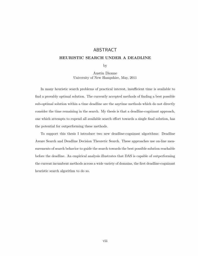
ABSTRACT
HEURISTIC SEARCH UNDER A DEADLINE
by
Austin DionneUniversity of New Hampshire, May, 2011
In many heuristic search problems of practical interest, insufficient time is available to
find a provably optimal solution. The currently accepted methods of finding a best possible
sub-optimal solution within a time deadline are the anytime methods which do not directly
consider the time remaining in the search. My thesis is that a deadline-cognizant approach,
one which attempts to expend all available search effort towards a single final solution, has
the potential for outperforming these methods.
To support this thesis I introduce two new deadline-cognizant algorithms: Deadline
Aware Search and Deadline Decision Theoretic Search. These approaches use on-line mea-
surements of search behavior to guide the search towards the best possible solution reachable
before the deadline. An empirical analysis illustrates that DAS is capable of outperforming
the current incumbent methods across a wide variety of domains, the first deadline-cognizant
heuristic search algorithm to do so.
viii

CHAPTER 1
INTRODUCTION
1.1 Heuristic Search
Heuristic search is a commonly used method of problem solving in artificial intelligence
applicable to a diverse set of complex problems such as path-finding, planning, and other
forms of combinatorial optimization. The method involves constructing a graph or tree of
problem states reachable from some starting state and using domain specific knowledge in
order to guide a search through that graph to find solution states. Often there is a cost
associated with each of these solution paths and the goal of search is to find a solution with
minimum cost.
In order to apply search algorithms, a problem must be capable of being characterized
in the following format: s0, the starting state of the problem; expand(s), a function which
takes a problem state s and returns a list of pairs (schild, c) representing the states reachable
from s by taking an action with associated cost c; goal(s), a predicate which can be used
to identify solution states of the problem.
Heuristics are functions which take a particular problem state and return some sort of
information about that state that can be used to help guide a search. One common heuristic
used is h(s), a function which takes a problem state s and returns an estimate of cost-to-go
to the best solution reachable from s.
Using this heuristic estimate, the overall quality of the best solution under a particular
state s can be estimated. This is typically noted as: f(s), the estimated cost of the best
solution under problem state s. This value is calculated as f(s) = g(s) + h(s), where g(s)
1

represents the cost incurred so far by actions taken leading from the starting state s0 to
state s. Classical heuristic search algorithms such as A* [5] will expand states in order of
minimum f(s) until a goal state is selected for expansion.
The characteristics of a particular heuristic used in a search can have important implica-
tions. For example, when using an admissible heuristic, one which never over-estimates the
cost-to-go for a particular state, an algorithm which sorts on minimal f(s) such as A* can
be guaranteed to return an optimal solution. However, finding admissible heuristics which
are also accurate in their estimates across a search space is often a very difficult problem.
Heuristic inaccuracy may lead to a larger number of states having to be expanded during
the search. In many cases when optimal solutions are not required (such as in deadline
driven heuristic search) it may make sense to use heuristics which are more accurate at the
cost of being inadmissible (potentially overestimating).
In many domains, often called unit-cost domains, actions all have an equal associated
cost. Other domains may have different costs associated with different actions. When
dealing with these non-unit-cost domains, several methods described by this work make use
of an additional heuristic: d(s) - the estimated distance-to-go to the best solution under
s (in terms of actions, not cost). One will find that when dealing with heuristic search
under deadlines, the distance-to-go heuristic is of key importance in domains which are
non-unit-cost.
1.2 Search Under Deadlines
For many problems of practical interest, finding optimal solutions using an algorithm such
as A* can not be done in a reasonable amount of time. There are many applications in
which solutions must be returned within strict time deadlines and suboptimality is tolerable.
In robotics applications such as autonomous vehicle navigation, plans must be completed
timely enough that the agent can react successfully in a realistic environment. In computer
games, players expect AI controlled agents to behave in real time, limiting the time for
2
planning their actions to very small windows. At every International Planning Competition,
bounds are given on the amount of computation time for competing algorithms to find
solutions and in each competition many algorithms fail to solve problems within the time
given.
To address this problem, sub-optimal search with an inadmissible or weighted heuristic
can often be used to reduce the amount of time necessary to find a solution. However,
while many algorithms have been proposed which can bound the level of suboptimality and
find a solution as fast as possible subject to that bound, not many algorithms have been
proposed which can do the opposite: bound the amount of search time available and find
the cheapest solution possible subject to that bound. Algorithms of the latter type are
sometimes referred to as contract algorithms, where the “contract” is the amount of time
given to the search to find a solution.
The currently accepted method for performing heuristic search under deadlines is to
use an “anytime” approach. An anytime search algorithm is one that first finds a sub-
optimal solution, likely in a relatively short amount of time, then continues searching to find
improved solutions until the deadline arrives or the current solution is proved to be optimal.
This approach is appropriate in the case when the deadline is unknown. However, when
the deadline is known, we propose that a deadline-cognizant approach is more appropriate
and may lead to better results. We will discuss this further in Chapter 2 after the survey
of the anytime approaches.
1.3 Outline
• Chapter 2 surveys the current anytime approaches used for solving heuristic search
under deadlines as well as the only known previous proposals for deadline-cognizant
contract search algorithms. Desired features of a new approach as well as problems a
new approach will face are outlined.
• Chapter 3 describes one algorithm we propose for solving the problem of search under
3
deadlines: Deadline Aware Search (DAS). This approach uses online measures of
search behavior to estimate the reachability of goals under particular states in the
search space. Only those states with goals deemed “reachable” are explored. A
model of using single-step heuristic error to construct corrected heuristic estimates is
introduced. Empirical results are shown that illustrate that DAS can outperform the
currently accepted anytime solution ARA* in many domains.
• Chapter 4 describes another algorithm we propose which extends the concept of DAS
to be more flexible and model the uncertainty inherent in the decision making problem
of search under deadlines: Deadline Decision Theoretic (DDT) search. This approach
addresses the concept of risk by using probabilistic estimates of reachability and ex-
pected solution quality. An extension to the single-step error model is proposed which
allows for on-line construction of probabilistic estimates of true distance and cost-to-
go. Results show potential for this approach, but do not surpass the results from the
simpler DAS.
• Chapter 5 summarizes the conclusions we have drawn from this work and describes
the many future directions in which this research could continue.
4

CHAPTER 2
BACKGROUND
This chapter summarizes the background of the problem, the incumbent approaches, and
the desired features and issues faced by a new approach. The incumbent approaches include
a short survey of the relevant anytime algorithms as well as descriptions of the only other
deadline/contract search algorithms proposed to date. We describe the desired features
of and issues faced by a new approach, which will motivate the approaches taken by the
algorithms proposed in Chapters 3 and 4.
2.1 Background
Since the introduction of A* [5] and its ability to find optimal solutions given an admissible
heuristic, many methods for reducing search time at the cost of solution quality have been
proposed. One widely used method of trading solution quality for search time is the use of
weighted admissible heuristics such as in Weighted A* [10]. By constructing an inadmissible
heuristic by multiplying admissible heuristic values by a weight factor w, the cost of the
solution found by a best-first search can be bounded by 1+w times the cost of the optimal
solution. Several algorithms have since been proposed which use a combination of admissible
and inadmissible heuristics in order to find such a bounded suboptimal solution as fast as
possible [19].
In practice, however, one may find that it is often more useful to solve the opposite prob-
lem: bounding the time allowed before a solution is needed and finding the best solution
possible within that time. Despite the wide range of applications of time bounded search,
5
there exists a surprisingly small amount of work which directly addresses the problem. In
our literature review we discovered only two deadline-cognizent approaches which directly
consider an impending deadline during the search. While interesting, neither of these ap-
proaches work very well in practice on a variety of problems with real time deadlines.
The most typical solution applied to the problem of searching under a deadline is to
use an anytime approach. These approaches do not directly consider the time remaining
in the search and we therefore call them deadline-agnostic. Despite their ignorance of
the impending deadline, anytime algorithms currently provide the best performance for the
problem and represent the incumbent solution we aim to beat with a new deadline-cognizant
approach.
2.2 Existing Deadline-Agnostic Approaches
The most common solution used when searching under a deadline is to use one of the various
anytime algorithms. These algorithms first find a suboptimal solution relatively quickly and
then spend the rest of the search time finding a sequence of improved solutions until the
optimal solution is found. They are referred to as “anytime” because they can be stopped
at any point, such as when the deadline has arrived, and return the best solution found
thus far.
2.2.1 Survey of Anytime Methods
There exists a large number of different anytime algorithms. This section provides a brief
survey of the modern approaches.
Anytime Weighted A*
The Anytime method was first formalized in Hansen et al.(1997) [4], in which they proposed
a method of converting any inadmissible search algorithm into an anytime algorithm. In
particular they present an anytime version of Weighted A* that is later analyzed in more
6
depth and named Anytime Weighted A* (or AWA*) by Hansen et al.(2007) [3]. This method
uses a weighted A* search to find an initial incumbent solution and then continues searching
using the weighted heuristic. The cost of the current incumbent solution is used as an upper
bound on estimated solution quality to prune states based on the unweighted version of the
admissible heuristic. As the search progresses, the lowest unweighted f value of any state
on the open list is tracked and used as a lower bound on the quality of the optimal solution.
Eventually these two bounds converge and the currently held incumbent solution is proven
to be optimal.
In their experiments, Hansen et al. have shown that by using the appropriate weight for
a particular domain and heuristic, AWA* has the capability of finding an optimal solution
both faster and using less memory than A*. They point out the fact that often AWA*
finds the optimal solution fairly early in the search and spends much of the remaining
time proving that the current incumbent is optimal. While noting that using the correct
weights also provides good anytime performance, there was no analysis showing the quality
of individual solutions found during a search over time or how sensitive the algorithm is to
weight selection. This was analyzed in more depth later by Thayer et al.(2010) [17].
Anytime Repairing A* (ARA*)
Likhachev et al.(2003) [8] introduced a variation of Anytime Weighted A* which they named
Anytime Repairing A*. This algorithm, similar to AWA*, performs an initial weighted A*
search to find a starting incumbent solution and then continues searching to find a sequence
of improved solutions eventually converging to the optimal. One difference from AWA* is
that after each new solution is found, the weight of the search is reduced by some predefined
amount. Also, this algorithm postpones the expansion of duplicate states until the discovery
of the next improved solution. Whenever a better path to a particular state that was already
expanded is found, it is inserted into a separate list of inconsistent states called INCONS.
Once the next solution is found, all states from the INCONS list are added to the open list
and may be re-expanded upon the next iteration. Their intention by delaying the expansion
7

of these duplicate states is to save effort in re-expanding states to propagate new g values
while still maintaining the sub-optimality bound of the current weighted search iteration.
This method boasts of improved performance over AWA* in the domains of robotic
motion and path planning. However, further work by Hansen and Zhou (2007) calls into
question the benefits of using the algorithm in general. In other domains, Hansen and Zhou
showed that both the features of decreasing weight and delayed state re-expansions either
had little positive effect or in some cases negative effects on performance. They suggest that
decreasing the weights may improve performance in some cases, but the benefits are less
significant if appropriate starting weights are selected. They also suggest that the delayed
re-expansion benefits of ARA* may only provide a significant improvement in domains with
a large number of similar solutions with close f values, resulting in many more duplicate
states. Contrary to this criticism, a very in-depth analysis was later performed by Thayer et
al.(2010) [17] which showed that the general approach of ARA* was consistently beneficial.
Restarting Weighted A* (RWA*)
Richter et al.(2009) [11] proposed a modification to the weighted anytime approach which,
while possibly appearing counter-intuitive at first, often results in better anytime perfor-
mance. Their algorithm, Restarting Weighted A* (RWA*) performs an anytime weighted
search similar to AWA*, while decreasing the weight after each solution is found similar to
ARA*, with the additional action of clearing the open list after each search iteration. The
states from the open list are saved in a separate seen list in order to be reused for heuristic
calculations and state generation overhead.
In some search domains, particularly Planning Domain Definition Language (PDDL)
planning, this action of restarting the search at each iteration has a surprisingly positive
effect on the results, causing better quality solutions to be returned faster during the search.
By restarting the search, errors which may have been made early in the search with a
significant impact on the final solution cost can be corrected. Without restarting the search,
these errors are often not corrected quickly due to the bias for expanding states with low h
8
values because of the weighted heuristic. In other domains the results remained competitive
with the non-restarting anytime algorithms. It was shown that the restarting approach did
not cause any significant negative effects on performance in any domain that was evaluated.
Beam Stack Search
Zhou et al.(2005) [20] proposed a new anytime adaptation of beam search which they called
Beam Stack Search. This algorithm uses backtracking in addition to a typical beam search
in order to continue searching for improved solutions until the optimal solution is found.
Typically beam search expands only a subset of the most promising states at each level of the
search, only in this case those states which were not selected for expansion are maintained
in data structure they call the Beam Stack. The algorithm is assumed to be started with an
incumbent solution which is used as an upper bound on solution quality. States which have
an admissible f value greater than the current upper bound are never expanded. When
the search finds a layer in which no states have an f value lower than the current upper
bound, the algorithm begins backtracking using the data stored in the Beam Stack. During
backtracking, it forces each layer to select a new set of states for expansion by adjusting
bounds on the f values. During the search the algorithm will encounter new solutions,
guaranteed to be improvements on the previous solution due to the pruning method. The
current upper bound on solution quality will be lowered and the search will continue until
it has exhausted the entire beam stack, proving that the current solution is optimal.
Beam Stack Search has the benefit of avoiding the weighted A* approach which suffers
from a need to know an appropriate weight schedule to apply in order to exhibit good any-
time performance. Similar to beam search it also has a controlled usage of memory. In [20]
they perform experiments on several STRIPS planning domains and show an improvement
in results over the previous methods.
9
Anytime Window A*
Aine et al.(2007) [1] introduced an anytime algorithm called Anytime Window A* which,
similar to Beam Search, does not depend on weighted heuristics. In their algorithm, a
series of iterative searches are performed in which each search has a certain window size
used to select states for expansion. For a given window size w, only those states whose
depth is within w of the maximum depth of any state expanded so far in the search are
taken into consideration. Within this sliding window, states are selected in best-first order.
Citing Pearl (1984) [9], Aine et al. claim that heuristic error is typically dependent on
this distance and by examining states within a distance window, tighter pruning can be
obtained. The window size increases and a solution is found at each iteration until the
search eventually exhibits the behavior of A* and converges on the optimal solution.
In their paper, Anytime Window A* was tested against other anytime algorithms in the
domains of the Travelling Salesman Problem and 0/1 Knapsack problem, presenting results
only in terms of state expansions and not actual search time. They show that Anytime
Window A* outperformed the other algorithms both in terms of average solution quality
and the percentage of solutions which converge to the optimal cost, over time.
d-Fenestration
An improvement to Anytime Window A* was proposed by Thayer et al.(2010) [17] which
both allows it to solve more problems and helps it converge to optimal solutions faster. In
the paper, they note that the depth of a particular state is always inversely proportional to
the distance from that state to its respective best goal. They therefore suggest redefining
the method used for windowing from selecting all states with a depth within the window
size of the maximum depth of any state to selecting all states with a value of d(s) within
the window size of the minimum d(s) of any state.
Thayer et al. also acknowledge that in many domains, unlike those evaluated in the
original Anytime Window A* paper, it is quite possible that many of the iterations of
10
Anytime Window A* will not return an improved solution. To address this, d-Fenestration
employs a method of increasing the window size at an increasing rate as iterations are
performed which do not return new solutions.
Results on the gridworld and robot pathfinding domains clearly illustrate the improve-
ments made to Anytime Window A* which allow it to handle a wider class of problems and
improve performance.
2.2.2 Comparison of Anytime Methods
Thayer et al.(2010) [17] recognized the need for a comprehensive evaluation of the anytime
methods across a wide variety of domains. They classified the weighted anytime approaches
into three basic categories: continuing, restarting, and repairing, and compared the use of
various bounded sub-optimal search algorithms as the base for the anytime implementations.
Finding that the choice of sub-optimal search algorithm rarely had a significant effect on
the performance of the general anytime framework they chose to use Explicit Estimation
Search ([18]) as the base for their anytime comparisons.
Thayer et al. then compared the three weighted A* based anytime approaches with
Beam Stack Search and their improved d-Fenestration version of Anytime Window A*
across a large set of commonly used benchmark domains. Somewhat contrary to the findings
of Hansen et al.(2007) [3], from their experiments it is clear that the repairing anytime
framework first defined by Likhachev et al.(2003) [8] had the best general performance
across all domains. Following this conclusion, we chose to compare the results of our
deadline-cognizant approaches with Anytime Repairing A*.
One important conclusion was drawn from their results on the Traveling Salesman Prob-
lem. On this problem d-Fenestration had difficulty finding the first solution for short cut-off
times but once found the results clearly beat out the other anytime algorithms. This illus-
trates the fact that for specific deadlines there may be different anytime algorithms which
return the best results and no a single best approach may exist for a range of deadlines.
11

2.2.3 Criticism of the Anytime Approaches
The anytime approaches are appropriate for solving heuristic search problems in which there
is a time deadline which is unknown. While they can certainly be applied to the problem of
heuristic search with known time deadlines, we argue that the time remaining in the search
is a significantly useful piece of information and there must exist a better approach which
takes the search time remaining into direct consideration. There are two essential problems
with the anytime approach which a new deadline aware approach should address:
1. Effort is wasted in finding the sequence of incumbent solutions during
the search. Despite the fact that the best solution found so far during a search can be
used for pruning the state space as the search continues, when the search terminates only
a single solution is returned. We argue that all effort should go towards finding that single
best solution. There is no need to be safely incrementing the quality of an incumbent
solution when time remaining in the search is known. However, we must be somewhat
careful with this argument because it is not easy to measure exactly how much effort is
wasted. For example, it has been shown that using this incremental approach where a
sequence of improved incumbent solutions is used for pruning can actually result in finding
optimal solutions faster and using less memory than A* [3]. This is, however, not typically
the case.
2. The weighted A* based anytime approaches, which currently exhibit the
best overall anytime performance, depend heavily on the weight schedule spec-
ified at the start of the search. It has been shown that the weighted A* based anytime
approaches can work well with well-selected weight schedules for particular problems and
heuristics. It has yet to be shown how to select a single weight schedule that can per-
form well over a large range of deadlines for a particular problem and heuristic, if possible.
There is also the distinct possibility that choosing an inappropriate weight may result in
the search not finding the initial incumbent solution within the deadline. It has been shown
12
that in some domains simply increasing the weight used in the search may only decrease the
amount of time necessary to find a solution up to a certain point before it begins to have
a negative impact on search time. There exists no clear way to choose an optimal weight
schedule for a particular problem and a particular deadline other than training off-line on
similar problems.
2.3 Existing Deadline-Cognizant Approaches
In our research we found only two previous proposals of algorithms that are deadline-
cognizant. Neither of these algorithms performed well in practice, which is possibly the
reason that they have not caught on and anytime search remains the most used approach
to the problem.
2.3.1 Time-Constrained Heuristic Search (1998)
Hironori et al.(1998) [6] proposed a contract algorithm, Time Constrained Search, based
on weighted A*. It attempts to measure search behavior and adjust accordingly in order
to meet the deadline while optimizing solution quality. They perform a best-first search on
f ′(s) = g(s)+h(s)·w, where g(s) represents the cost of the path explored thus far, h(s) is the
heuristic estimate of cost-to-go, and w is a weight factor that they adjust dynamically. They
take advantage of the fact that increasing the weight of the heuristic value generally has the
effect of biasing search effort towards states that are closer to goals, therefore shortening
the amount of search time necessary to return a solution.
They determine how to properly adjust the weight using a concept they call search
velocity. They define the distance D as the heuristic estimate of cost-to-go of the starting
state: D = h(sstart). They then use the time bound T assigned to the search to calculate
a desired “average velocity” V = D/T . During the search they use the time elapsed t
and the minimum h(s) value for any state generated thus far hmin in order to calculate an
“effective velocity” v = (D − hmin)/t. If the effective velocity falls above/below a selected
13

tolerance from the desired average velocity, the weight applied to h(s) when calculating
f ′(s) is adjusted accordingly by subtracting/adding a predetermined value of ∆w.
This approach relies on several parameters that have a significant impact on algorithm
performance, such as the upper and lower bounds on average search velocity and the value
of ∆w. Several important questions, such as how often (if ever) to re-sort the open list
or if there is any sort of minimum delay between weight adjustments, are not specified
and attempts to contact the authors to resolve these issues were unsuccessful. While their
empirical analysis illustrates the quality of solutions found over a range of real-time deadlines
(with the contract specified in seconds of computation time), no comparisons were made
to other approaches. Despite our best efforts to implement and optimize this algorithm
we were unable to create a real-time version that was at all competitive with the anytime
approaches (Anytime Weighted A*, ARA*) for the domains we tested.
2.3.2 Contract Search (2010)
Contract Search [2] attempts to meet the specified deadline by limiting the number of state
expansions that can be performed at each depth in the search tree. The algorithm is based
around the following insight into A* [5] search on trees: for A* to expand the optimal
goal, it need only expand a single state along the optimal path at each depth. The idea
behind Contract Search is to expand only as many states as needed at each depth in order
to encounter the optimal solution. In practice, we obviously do not know how many states
need to be expanded at each depth in order to find an optimal solution. We can assume
that the more states we expand at a given depth, the more likely we are to have expanded
the optimal state. Contract search therefore attempts to maximize the likelihood that an
optimal solution is found within the deadline by maximizing the likelihood that the optimal
state is expanded at each depth, subject to the sum of expansions over all depths being
less than the total expansions allowed by the deadline. They also propose a method of
minimizing the expected cost of the solution found (rather than maximizing the chances of
finding the optimal solution), although they themselves do not evaluate this modification.
14
The algorithm has two phases: determining off-line how many states should be consid-
ered at a given depth, k(depth), and then efficiently using this information on-line in an
A*-like search. Rather than a single open list sorted on f(n), contract search maintains a
separate open list for each depth, reminiscent of beam search. Each of these per-depth open
lists tracks the number of states it has expanded and becomes disabled when this reaches
its k(depth) limit. At every iteration of the search, the state is expanded with the smallest
f(n) across all open lists that have not yet exhausted their expansion budget. For very
large contracts, this will behave exactly like A*, and for smaller contracts it approximates
a best-first beam search on f(n).
Determining the number of states that maximizes the probability of success or minimizes
the expected solution cost can be done offline, before search. To do so, we need to know
a probability distribution over the depths at which goals are likely to appear, the average
branching factor for the domain, and the likelihood that the optimal state at a given depth
will be expanded within a fixed number of states. All of these can be determined by
analyzing sample problems from the domain, or they can be estimated. Given these values,
the number of states to expand at each depth for a given contract can be solved for using
dynamic programming. These values are then stored for future use.
The largest contract considered by Aine et al.(2010) [2] is 50,000. In many practical
problems and the evaluation done in this thesis, we will be considering search deadlines of
up to a minute, which for our benchmark domains could mean more than five million states.
This is problematic because the time and space complexity of computing these values grows
quadratically in the size of the contract. Aine suggested approximating the table by only
considering states in chunks, rather than a single state at a time. This cuts down on the
size of the table and the number of computations we need to perform to compute it. In
the results presented in this thesis the resolution was selected such that the tables needed
could be computed within 8 GB of memory. Computing the tables typically took less than
eight hours per domain.
15
2.4 Desired Features of a New Approach
2.4.1 Optimality and Greediness
At any time during the search there exists an open list of states that represents the search
frontier. From this list of states, a search algorithm must choose which to expand next based
on some set of rules. In general, a deadline-cognizant heuristic search algorithm wishes to
expand the state under which the best solution resides which can be found within the time
remaining. It is desirable that if enough time is given to the search it would behave similarly
to A* and find the optimal solution. Conversely, if too little time is given to the search to
allow for any deliberation among states, quality should be ignored and the search should
resort to the fastest method of finding a solution possible: a greedy search on d(s).
2.4.2 Parameterless and Adaptive
Many of the existing approaches to deadline search described in this chapter require careful
setting of algorithm parameters, such as the weight schedules chosen for ARA* or the
many parameters required for Time-Constrained Search. Contract Search requires specific
knowledge about problem instances and significant off-line computation time for computing
the k(depth) values. When facing search problems with deadlines, one can not always
assume that such luxuries will be available and a desirable approach would be one which is
parameterless and requires no off-line training to guarantee performance on a new instance
or domain.
2.5 Challenges for a New Approach
This section highlights the challenges that are faced by a deadline-cognizant approach in-
tending to exhibit the desired features from the previous section. These challenges are
addressed differently by both proposed algorithms DAS and DDT.
16
2.5.1 Ordering States for Expansion
For a deadline-cognizant algorithm to devolve to A* for sufficiently long deadlines (one of
the desired features of a new approach) it would have to expand nodes in a best-first order
on an admissible heuristic. However, admissible heuristics are typically less accurate and
lead to more states being expanded during the search in order to find an optimal solution,
which may not be desirable behavior when facing relatively shorter deadlines for which a
suboptimal solution is all that can be achieved.
Using an inadmissible, but possibly more accurate, heuristic has the benefit of causing
the search to be more depth oriented, because there will be a higher probability that a child
state of an expanded state will have a similar or better f value causing it to be selected for
expansion sooner. This is a well-known phenomenon and is the basis of weighting admissible
heuristics in an attempt to reduce search time. This approach may allow for reasonably
good sub-optimal solutions to be found much sooner, possibly making it easier to meet
deadlines. However, this comes at the sacrifice that the optimal solution will not be found
first for sufficiently large deadlines.
The following chapters will show that DAS uses an admissible f(s) heuristic in order to
guarantee A* behavior for long deadlines while relying on d(s) and a pruning strategy for
controlling the progress of the search, rather than a weighted cost heuristic. DDT constructs
heuristic values using belief distributions for d(s) and h(s), sacrificing admissibility for
rational search behavior.
2.5.2 Reachability of Solutions
The arguably more difficult question for deadline search is deciding which states have solu-
tions under them that are “reachable” and worth pursuing in the time remaining. Deciding
what is reachable and what is not is difficult due to the following two problems that must
be addressed by a deadline-cognizant approach.
1. The distance (in terms of search steps/state expansions) to reach a particular
17
goal is not known with certainty. The d heuristic can be used to estimate this distance,
but the accuracy of the estimate would have a significant impact on the ability of the search
to complete within the deadline. For example, assume that we have a perfect h heuristic
and therefore know exact f values for all states. The algorithm could therefore estimate
the number of expansions remaining before the deadline and select the best state to pursue
with a d value less than that number. However, if the d values of the best children under
each state do not consistently decrease by 1 after each expansion, it is possible that the
search would not reach that goal within the deadline and by the time this occurs, it may
no longer have enough expansions remaining to pursue any other path.
2. Error in the h heuristic causes the search to consider multiple paths to solu-
tions simultaneously. Due to errors in the heuristic estimate h, the f value of the best
child under a particular state is often higher than that of the parent state. Because of this
it is quite possible that the child state will not be the next selected for expansion based
on f . This child state will only be selected once either all better states have lead to dead
ends or the heuristic error has caused all their decendants’ f values to increase similarly.
We call this behavior of exploring several different paths somewhat simultaneously “search
vacillation”. Due to the vacillation of the search, the number of steps/expansions that will
be executed along any one path to a solution will typically be much less than the number
of expansions performed over a certain period of time.
Take for example the case in which the d heuristic is perfectly accurate. We can therefore
choose the best state from the open list with absolute certainty that the best solution under
that state can be reached within the time remaining. However, as states along the path to
that solution are expanded the children may often have larger f values than their parents.
If the search were to continue selecting states for expansion based on f , other paths will
be explored simultaneously, further reducing the number of expansions remaining in the
search. If the f values of the explored paths continue to rise, at some point there will be
states in the search that were previously ignored and now appear to lead to better solutions,
but whose goals will not be reachable in the time remaining.
18
It is therefore expected that a search that simply expands the state with minimal f
value and knows exact d values will concentrate most of its effort in the section of the search
space nearest the root, at the beginning of the search when there are enough expansions
remaining to find any particular goal if it were explored exclusively. Because expansions
will be spent along many paths in parallel due to the search vacillation, the number of
expansions remaining will decrease far faster than the d values of the states explored. It is
expected that at some point only one state will have a goal that is deemed reachable within
the expansions remaining and the rest of the search will be spent following that one path
without consideration of other, possibly better, solutions.
In Chapters 3 and 4 we will show that DAS and DDT confront this issue by measuring
the search behavior on-line and estimating the number of expansions which will be spent
searching on any particular possible solution path given the vacillation present in the search.
DAS chooses to use this model of search behavior to expand only those states which lead
to reachable solutions, while DDT considers the fact that all states will have some amount
of risk of not finding an improved solution if explored.
19
CHAPTER 3
DEADLINE AWARE SEARCH
(DAS)
In this chapter we propose a new deadline-cognizant algorithm that uses on-line measures
of search behavior to estimate which states lead to reachable solutions within the deadline
and pursues the best of those solutions. A method of measuring heuristic error on-line and
using those errors in a model to construct corrected heuristic estimates is proposed and
used in DAS. Algorithm performance is evaluated using real-time deadlines on a variety of
domains, illustrating a general improvement over the incumbent anytime methods.
3.1 Motivation
Deadline Aware Search (DAS) is a simple approach, motivated directly from the objective
of contract search. It expands, of all the states deemed reachable within the time remaining,
the one with the minimum f(s) value. DAS uses the original admissible heuristic f(s) rather
than some weighted or corrected heuristic f(s). This allows for DAS to devolve to A* in the
case of sufficiently large deadlines and did not result in a significant decrease in performance
for shorter deadlines when evaluated empirically. Pseudo-code of the algorithm can be seen
in Figure 3-1. Reachability is a direct function of that state’s distance from its best possible
solution. Rather than use the (commonly admissible) heuristic value d(s) for estimating
this distance, DAS uses a more accurate corrected heuristic d(s).
20

Deadline Aware Search(starting state, deadline)1. open ← {starting state}2. pruned ← {}3. incumbent ← NULL4. while (time) < (deadline) and open is non-empty5. dbound ← calculate d bound()6. s← remove state from open with minimal f(s)7. if s is a goal and is better than incumbent8. incumbent ← s
9. else if d(s) < dbound10. for each child s′ of state s11. add s′ to open12. else13. add s to pruned14. if open is empty16. recover pruned states(open, pruned)17. return incumbentRecover Pruned States(open, pruned)18. exp ← estimated expansions remaining19. while exp > 0 and pruned is non-empty loop20. s← remove state from pruned with minimal f(s)21. add s to open
23. exp = exp −d(s)
Figure 3-1: Pseudo-Code Sketch of Deadline Aware Search
When there is not enough time to explore all interesting paths in the search space,
it makes sense to favor those paths which are closer to solutions. One result of using an
admissible heuristic h(s) when ordering states for expansion is that often the best f value of
the child states under a particular state s will be higher than the value of f(s). Assuming the
heuristic error is distributed approximately uniformly across a search space, the states that
are farther from solutions have the potential of experiencing this increase in f value more
often before reaching their respective solutions than states that are closer. Also, because
search spaces generally increase exponentially, states that are farther from solutions also
generally have larger sub-trees lying beneath them. Intuitively, when one is faced with an
approaching deadline and a limit on which states can be expanded, it makes sense to decide
21
not to explore states that have a higher variability in f value and lead to a larger increase
in search space to explore.
3.2 Algorithm Description
Deadline Aware Search (DAS) performs a standard best-first search on f(s), breaking ties
on higher g(s). At each expansion, it estimates the “reachable” solution distance dmax. If
the state selected for expansion has a corrected distance-to-go value d(s) greater than this
maximum value, then it is inserted into the pruned list and not expanded. Otherwise, the
state is expanded and its children are added to the open list as usual.
It is possible that at some point during the search there are no more states to expand
because all states have been moved to the pruned list. This would be an indication that
given the current search behavior, if the search were to continue, it is not expected that a
solution will be reached. In this case, the Recover Pruned States method is invoked, which
attempts to reinitialize the search such that solutions will once again appear reachable.
When this occurs, DAS will reinsert a subset of the best states, those with minimal f(s)
values, from the pruned list into the open list. The subset is chosen such that the sum of
d(s) for all recovered states s is less than the estimated number of expansions remaining
in the search. At this time, the search behavior will have changed so drastically that the
current model used in calculating dmax will also be reset. The search can then continue
from this point.
3.3 Correcting d(s)
To address the problem of inaccurate (and often admissible/underestimating) d(s) heuris-
tics, DAS constructs a corrected heuristic d(s). There are several methods of calculating
such a heuristic, including using artificial neural networks or least mean square error ap-
proximations to determine an appropriate correction for the admissible heuristic. These
methods, however, typically require training to be performed off-line on similar problem
22

instances, which is undesirable. On-line versions of these methods exist, but do not seem
to perform as well as their off-line counterparts [15]. For this research we determined our
own on-line correction method for heuristics, described in the following sections.
3.3.1 One-Step Error Model
Ruml and Do (2007) [12] introduced a method of measuring heuristic error at each state
expansion on-line and using those measurements to construct corrected heuristics h(s) and
d(s). We correct that model by adding additional (necessary) constraints to the calculation
of one-step error, introducing a new definition for d(s) which accounts for the recursive
nature of introducing additional steps into the solution path, and providing more theoretical
background including a proof that the model is correct when certain facts about the search
space are known.
One thing that is known about the actual search distance-to-go for a particular state s
is that the optimal child oc(s), the next state along the optimal path to a solution under s,
will have an actual distance-to-go d∗(oc(s)) of exactly one less than the actual distance to
go of its parent d∗(s).
We therefore define the one-step heuristic error ǫd as the difference between the estimated
distance-to-go of the optimal child under s and the expected distance-to-go.
ǫd = d(oc(s))− (d(s)− 1) (3.1)
Figure 3-2 shows a simple grid-world navigation problem where the paths explored and
the one-step errors in d are displayed. This assumes the use of the Manhattan Distance
heuristic, calculated for any grid position (x, y) as: d(s) = |x−xgoal|+|y−ygoal|, representing
the distance to the goal assuming there were no blocked positions.
We require that the optimal child selected for this calculation not include the parent
state of s. This implies that oc(s) represents the child along the optimal path to a solution
not including the path back through the parent state. This requirement has two important
implications. One is that states with no children other than the reverse action back to their
23

Figure 3-2: Gridworld One-Step Heuristic Error Example (Manhattan Heuristic)
parent will have no associated ǫd, evident in locations (0,2) and (0,4) of Figure 3-2. More
importantly, the other implication is that for any state s, the sum of d(s) and all one step
errors along an optimal path to the goal under s,∑
n∈p goal
ǫdn, is equal to the actual distance
d∗(s).
This can be seen in Figure 3-2 by starting at any position, taking the d value for that
position, then adding up the one-step errors along the best path from that position to the
goal. One example of this can be seen by starting at location (2,3) where d(s) = 8 and
d∗(s) = 12. Following the best path to the goal passes through two locations (4,4) and (4,3)
with one-step errors ǫd = 2. All other steps along this path have a one-step error of zero
and Equation 3.2 holds, as 8 + 2 + 2 = 12.
Theorem 1 For any state s with a goal beneath it:
d∗(s) = d(s) +∑
n∈s goal
ǫdn (3.2)
where s goal is the set of states along an optimal path between the state s and the goal,
including s and excluding the goal.
Proof: The proof is by induction over the states in s goal. For our base case, we show
that when oc(s) is the goal,
24
Equation 3.2 holds:
d∗(s) = d(s) +∑
n∈s goal
ǫdn
= d(s) + ǫds because s goal = {s}
= d(s) + 1 + d(oc(s))− d(s) by Eq. 3.1
= d(s) + 1− d(s) because d(oc(s)) = 0
= 1
As this is true, the base case holds.
Now for an arbitrary state s, by assuming that Equation 3.2 holds for oc(s), we show
that it holds for s as well:
d∗(s) = 1 + d∗(oc(s)) by definition of oc
= 1 + d(oc(s)) +∑
n∈oc(s) goal
ǫdn by assumption
= d(s) + ǫds +∑
n∈oc(s) goal
ǫdn by Eq. 3.1
= d(s) +∑
n∈s goal
ǫdn
�
An example of why the requirement is necessary can be seen in Figure 3-2 at location
(4,3). Without the requirement the value of ǫd would be zero, as a step back to the parent
location (4,4) would be considered the best child as it reduces the value of d by one as
expected. By disallowing (4,4) in selecting the best child, the state (4,2) must be selected,
resulting in a one-step error of 2, which as we have shown is necessary for Equation 3.2 to
hold.
Calculating Corrected d(s): d(s)
Using the proposed one-step error model we can construct a new heuristic d(s) from the
original d(s) that better estimates the true distance-to-go d∗(s).
25

We first define the mean one-step error ǫd along the path from s to the goal as:
ǫd =
∑
n∈s goal
ǫdn
d∗(s)(3.3)
Using Equations 3.2 and 3.3, we can define d∗(s) in terms of ǫd.
d∗(s) = d(s) + d∗(s) · ǫd (3.4)
Solving Equation 3.4 for d∗(s) yields:
d∗(s) =d(s)
1− ǫd(3.5)
Another way to think of Equation 3.5 is as the closed form of the following infinite
geometric series that recursively accounts for error in d(p):
d∗(p) = d(p) + d(p) · ǫd + (d(p) · ǫd) · ǫd + . . . (3.6)
= d(p) ·
∞∑
i=1
(ǫd)i (3.7)
In this series, the term d(s) · ǫd represents the number of additional steps necessary due
to the increase in d over the first d(s) steps. However, each of these additional steps will also
incur a mean one step error of ǫd, resulting in the next term of (d(s) · ǫd)ǫd. This continues
on recursively for an infinite number of terms. This series converges to Equation 3.5 if
ǫd < 1. This will always hold for paths that lead to goal states, as a mean one step error
greater than one would mean that the d value along that path never reached zero, implying
that the path never reached a goal.
Given the current estimate of ǫd, ǫestd , we define the corrected heuristic value d(s) as
follows:
d(s) =d(s)
1− ǫestd
(3.8)
26

Calculating Corrected h(s): h(s)
Using the one-step error model we can also construct an estimate of true cost-to-go h(s). In
DAS we chose not to use a corrected heuristic value for h(s) because it did not significantly
improve performance for shorter deadlines and for longer deadlines it sacrifices optimality.
Regardless, we cover it in this section as the method has applications in search problems
other than contract search.
Analogously to d(s), there is an expected relationship between the true cost-to-go esti-
mates of a parent and its optimal child oc(s), given the cost of transitioning from s to oc(s),
c(s, oc(s)).
h∗(s) = h∗(oc(s)) + c(s, oc(s)) (3.9)
This allows us to define the single-step error in h as:
ǫh = (h(bc(p)) + c(p, bc(p)))− h(p) (3.10)
As in Equation 3.2, the sum of the cost-to-go heuristic and the single-step errors from a
state s to the goal equals the true cost-to-go:
h∗(s) = h(s) +∑
n∈s goal
ǫhn (3.11)
Assuming that we know the true distance-to-go d∗(s), we can calculate the mean one-step
error ǫh along the optimal path from p to the goal as:
ǫh =
∑
n∈s goal
ǫhn
d∗(s)(3.12)
Solving for∑
n∈s goal
ǫhn and substituting into Equation 3.11,
h∗(s) = h(s) + d∗(s) · ǫh (3.13)
Using Equation 3.5 to calculate d∗(s) we have:
h∗(s) = h(s) +d(s)
1− ǫd· ǫh (3.14)
27

Using the current estimates of ǫd and ǫh, ǫestd and ǫesth , we define the corrected heuristic
value h(s) as follows:
Using Equation 3.5 to calculate d∗(s) we have:
h∗(s) = h(s) +d(s)
1− ǫestd
· ǫesth (3.15)
Application of One-Step Error Model
Using the one-step error model proposed in the last section requires estimating some un-
known features of the search space. At each state expansion the child residing on the
optimal path to the goal oc(s) is not known. We estimate this by selecting the “best” child
bc(s), that with minimal f(s) value, breaking ties on f(s) in favor of low d(s). Also, the
quantities ǫd and ǫh from the model are the mean one-step errors along an optimal path
to the goal. During a search, these values are unknown and must be estimated. We now
discuss two techniques for estimating ǫd and ǫh.
The Global Error Model assumes that the distribution of one-step errors across the entire
search space is uniform and can be estimated by a global average of all observed single step
errors. The search maintains a running average of the mean one-step errors observed so far,
ǫglobalh and ǫglobald . We then calculate d using Equation 3.5 and h using Equation 3.15.
The Path Based Error Model calculates the mean one-step error only along the current
search path, ǫpathd and ǫpathh . This model maintains a separate average for each partial
solution being considered by the search. This is done by passing the cumulative single-step
error experienced by a parent state down to all of its children. We can then use the depth
of the state to determine the average single-step error along this path. We then calculate d
using Equation 3.5 and h using Equation 3.15.
In either model, if our estimate of ǫd ever meets or exceeds one, we assume we have
infinite distance and cost-to-go. In theses cases algorithms may elect to break ties using
the original heuristic values, or some other means. DAS breaks ties in favor of smaller f(s).
Results of applying this one-step error model to the problem of sub-optimal search can be
28
seen in Thayer et al. [15], and will also appear in Jordan Thayer’s PhD dissertation.
3.4 Estimating Reachability
During the execution of Deadline Aware Search, the corrected distance-to-go estimates of
all states on the open list act as the primary tool for deciding which solutions are reachable
within the time remaining and which are not. Based on the time remaining in the search
and possibly other factors which intend to measure and account for the vacillation of the
search, a maximum tolerable distance-to-go dmax is calculated. This value represents the
furthest possible solution in terms of search steps which is deemed reachable within the
time remaining based on the current behavior of the search. We evaluated several different
methods of calculating dmax, which we describe in detail below.
In many of the methods described below, the rate of state expansions in the search
must be estimated. DAS estimates this value on-line by measuring the delta time over
the last N expansions and using a sliding window of these measurements to calculate the
average expansion rate. In practice, this estimate is seeded with a reasonable estimate of
the expansion rate to allow for the calculation of dmax before enough samples have been
collected. The results of DAS were not sensitive to this initial rate nor the value of N
(we used N = 10, 000 and exprate = 33, 333 in our empirical analysis). In the methods
described below we will assume that the estimated expansion rate exprate is known.
3.4.1 Naive
This method does not take into account the vacillation of the search whatsoever. Using the
current expansion rate dmax is simply calculated as the estimated number of expansions
remaining in the search before the deadline arrives:
dmax = (exprate) · (time remaining) (3.16)
One notable characteristic about this approach is that it does not intrude on the natural
behavior of the search until the moment when it is believed that there is only enough time
29
to follow a particular path exclusively in order to find a solution within the deadline. It is
expected that this results in most of the search effort occurring early in the search space up
to a point where only one path will have an acceptable distance-to-go estimate. This will
be followed to whatever goal lies beneath. Given the fact that there will be some vacillation
in the estimate of d(s), this is not generally safe search behavior.
3.4.2 Depth Velocity
This method calculates a “depth velocity” vd based on the behavior of the search thus far,
which has the intention of estimating the rate at which the search tree is deepening over
time. It is somewhat similar to the idea of search velocity first proposed in [6] but is used
here in a very different way. Three possible methods have been identified for estimating the
depth velocity:
Maximum Depth
vd =(maximum depth of any state generated)
(time elapsed)(3.17)
Recent Depth
vd =(average depth of the last k states expanded)
(time elapsed)(3.18)
Best Depth
vd =(average depth of the best k states on the open list)
(time elapsed)(3.19)
This velocity is then multiplied by the time remaining in order to estimate the search
distance remaining dmax.
dmax = (time remaining) · vd (3.20)
3.4.3 Approach Velocity
One could argue that the depth of a state does not directly correlate to the closeness of a
state to its respective best solution. This method addresses that issue by calculating an
“approach velocity” va based on the estimated proximity to solutions rather than the depth
in the search tree. It is calculated very similarly to depth velocity, the main difference
30

being that the estimated distance from the goal d is used instead of the depth of states.
Three possible methods have been identified for estimating approach velocity, synonymous
to those for depth velocity:
Closest Proximity
vd =(d(starting state)− (minimum d of any state generated))
(time elapsed)(3.21)
Recent Proximity
vd =(d(starting state)− (average d of last k states expanded))
(time elapsed)(3.22)
Best Proximity
vd =(d(starting state)− (avg d of best k states on the open list))
(time elapsed)(3.23)
This velocity is then multiplied by the time remaining in order to estimate the search
distance remaining dmax.
dmax = (time remaining) · vd (3.24)
One caveat with this approach is that for any methods that determine the appropriate
corrections for calculating d during the course of the search, d(starting state) may need to
be recalculated periodically in order to obtain an accurate estimate in relation to the d
values of newly expanded states.
3.4.4 Best Child Placement (BCP)
In general, the error in the h heuristic is to blame for vacillation during a search. The
reason that heuristic search must often evaluate several different possible solution paths
simultaneously is because after a particular best state is expanded, its children often do not
end up at the front of the open list because their f values have all increased. This method
attempts to estimate the vacillation in the search directly and use that expected vacillation
in order to estimate how many more expansions will occur along any one solution path
being considered.
31
At each expansion made in the search, the locations at which the child states are inserted
into the open list are recorded. The position of the best child pbest, that which ended up the
farthest forward in the open list, is added to a running average pbest. This average best child
placement represents, on average, how many expansions are necessary before that path will
be explored once again. This acts as a direct estimate of the search vacillation and can be
used to estimate how many expansions will therefore be spent on any particular path in the
search dmax.
dmax =(expansions remaining)
pbest(3.25)
The number of expansions remaining can be estimated in a method similar to that used
in Naive dmax, see Equation 3.16.
A potential benefit to this approach is that the search vacillation is measured directly,
whereas the velocity based approaches are somewhat more indirect. One problem with this
method is that is makes the assumption that all states ahead of the best child placed in
the open list, when expanded, will not place their best child states ahead of the first. This
assumption may lead to the under-estimation of the actual search vacillation.
3.4.5 Expansion Delay
Similar to BCP, this method attempts to measure the search vacillation directly in order
to estimate how many expansions will be spent on average along any particular path to a
goal in the search. However, this method attempts to address the strong assumption made
by BCP about the number of expansions made before reaching the best child placed in the
open list at the given position pbest.
Rather than measure the placement of the best child in the open list, this method
records the delay, in the number of expansions made, between when a child state is first
generated and when it is later found at the front of the open list and expanded by the
search. A running counter is maintained during the search that is incremented each time
an expansion is made. When child states are generated, they record the current expansion
32
number. Whenever a state is expanded, we calculate the expansion delay ∆e and add it to
the running average expansion delay ∆e, where
∆e = (current exp counter)− (exp counter at generation) (3.26)
The expected number of expansions spent along any particular path in the search dmax
can then be estimated similarly to BCP:
dmax =(expansions remaining)
∆e(3.27)
The benefit of using this approach is that it takes into consideration the effects of newly
generated states being placed into the open list ahead of previously generated states when
estimating search vacillation. It returns estimates of search vacillation that are strictly
higher than those calculated by BCP and are expected to be more accurate.
3.4.6 Comparison of Methods
It is difficult to define the “correct” values for dmax estimated by any of these methods.
The true distance that the search will explore down any particular path depends on the
behavior of the search in the time remaining. Because the value of dmax is used to prune
the search space, it will have an effect on that behavior and consequently, an effect on
the search vacillation and distance explored. This recursive relationship is expected and
the intention is that by using these methods on-line during the search, the estimation and
control will settle such that estimates of dmax do not fluctuate wildly and will instead follow
some smooth function approaching zero at the time of the deadline.
This relationship between control and estimation makes it difficult to evaluate the cor-
rectness of a particular approach any other way than empirically. Each approach was used
in DAS on several domains. Those methods that depend on parameter k were evaluated for
several different k. The Naive approach did not perform well in any case. For the velocity
based approaches the results were hit-or-miss. The best velocity based approaches were
the Recent Depth and Recent Proximity, however, the size of the window selected had a
33
significant impact on performance and there was no clear way to choose an appropriate size
given a domain/instance. Overall, the method that performed well most consistently was
Expansion Delay. We will show results for this approach in the following sections, as well
as more analysis into the behavior of dmax during a search.
3.5 Properties and Limitations
3.5.1 Optimality for Large Deadlines
One of the desired features for a contract search algorithm is that, given a long enough
deadline, the algorithm will devolve to A* and return a guaranteed optimal solution (given
an admissible heuristic). DAS has this property.
Theorem 2 Given a sufficiently long deadline d and assuming that the one-step error model
does not result in any states with d(s) = ∞, DAS will perform an equivalent search to A*
and return a guaranteed optimal solution.
Proof: Given that DAS performs a best-first search on an admissible f(s) and returns a
solution only when the state is selected for expansion, it behaves exactly like A* with the
exception of pruning states due to reachability. However, given a long enough deadline and
the use of any of the proposed methods for calculating dmax there will never be a state
selected for expansion such that d(s) > dmax. Therefore, the algorithm will behave exactly
as an A*. The proof that A* returns an optimal solution can then be directly applied. �
Admittedly, the minimum value of the deadline d necessary for this fact to hold depends
on the method of calculating dmax used as well as the characteristics of the search space
and could not be easily determined a priori.
3.5.2 Non-uniform Expansion Times
One assumption that DAS depends on is that the number of expansions remaining in the
search can be estimated. The expansion time depends on a two key operations: calculat-
34

ing the heuristic values for child states and inserting the child states into the appropriate
data structures. If, for example, the open list is implemented as a binary heap, then one
should expect that the cost of child state insertion should grow on the order of log(N) as
search progresses. More troublingly, some heuristics use costly methods such as calculating
minimum spanning trees or solving abstracted problems. The time required to calculate
such heuristics may depend on the current length of the partial solution and may vary
significantly across the search space. DAS currently uses a sliding window average on state
expansion time to try to account for some variation, however, it may not be enough to
handle the more complicated cases.
3.6 Experimental Results
We performed an empirical analysis over several benchmark domains in order to compare the
performance of Deadline Aware Search with that of Anytime Repairing A*, and Contract
Search. In each domain we tested over a range of deadlines covering around four orders of
magnitude.
In order to deal with the cases in which an algorithm does not return a solution within the
deadline, all algorithms are required to run an initial search algorithm we call “Speedier”.
Speedier search is a greedy search on d(s) in which duplicate states are detected and,
if already expanded, are ignored. This search completes very quickly, returning what is
typically a highly suboptimal solution that all algorithms can use as a starting incumbent.
Therefore any algorithm that fails to find an improved solution within the deadline will
return this sub-optimal Speedier solution. This both simplifies our analysis by assigning
a meaningful cost to the null solution and is a realistic implementation in the case of a
real-time application in which returning no solution is unacceptable.
For Anytime Repairing A* we evaluated the following range of initial weight settings:
1.2, 1.5, 3.0, 6.0, 10.0. The optimal setting found for the 15-Puzzle, Unit-Cost Grid-
World, Life-Cost Grid-World, and Dynamic Robot Navigation were 3.0, 3.0, 6.0, and 1.5,
35
respectively. In each plot the results for the top two weight settings are illustrated, as in
some cases there were settings which did not produce the best results overall but performed
better for a specific range of deadlines.
Contract Search uses the number of expanded states for its deadline, as originally pro-
posed, rather than a time cutoff like DAS. Similar to all other methods evaluated, Speedier
is run initially and the time elapsed is subtracted from the deadline. At this point the
time remaining is multiplied by the average state expansion rate, measured off-line for each
domain, in order to estimate the state contract to apply. The deadline is still measured
in seconds and when it arrives the algorithm is stopped like any other, keeping the best
solution found thus far.
3.6.1 Behavior of dmax and Pruning Strategy
The purpose of dmax in DAS is to act as a decreasing upper bound on the distance between
any state expanded and its respective best solution. This bound is intended to force the
search to progress forwards to meet a particular deadline when it would normally have
spent more time vacillating between different partial solutions sorting out the increasing
f(s) values. While it is difficult to justify what the “correct” value of dmax should be over
the course of the search, we can make a few reasonable expectations. The value should
represent a smooth function, as a large variability would cause unstable behavior in DAS.
Depending on the given deadline, the value should typically fall somewhere within the range
of current d(s) values such that some pruning will occur when necessary and not all states
will be pruned unnecessarily.
In order to evaluate the behavior of dmax relative to the d(s) of states expanded during a
Deadline Aware Search, we implemented a version which uses state expansions as a deadline
and records relevant information during the search. This way the overhead of recording
could be factored out of the analysis. Figure 3-3 contains the results of the analysis on a
single instance of unit-cost four-way gridworld navigation for a range of deadlines.
The plots illustrate the current value of dmax and the d(s) value of the expanded states
36
over the course of the search. The plots are shown for deadlines of 400k, 200k, 100k, and
50k expansions. DAS returned solutions of cost 2967, 3043, 3159, 3525, respectively. As a
reference point, A* completes for this instance after 402,220 expansions returning a solution
cost of 2967 and Speedier completes after 15,327 expansions returning a solution cost of
4041. The expansions taken by the initial Speedier search are included in the deadline. In
examining these plots, one should note that the red line representing dmax appears to spike
at various locations. With the exception of the start of the search, these points represent
when the reachability model is reset due to all states being pruned as “unreachable”. One
can recognize the points where solutions are returned as when d(s) = 0.
From the plots, one can see that for longer deadlines, the values of dmax effectively push
the search towards finding a solution with a somewhat significant amount of time (or in this
case, state expansions) remaining. After the first solution is found the search will have much
more strict bounds for pruning and one can see that the vacillation increases such that the
search repeatedly stagnates resulting in all states being pruned and the estimates of dmax
resetting. Despite the effort wasted in pruning and reinserting states, this does not need to
be interpreted as negative behavior. For example, looking at the plot for 50k expansions
one can see that during the search there are several points at which the model estimates
that no solution will be reachable given the current search behavior and the recover pruned
states method is invoked. It is thanks to this recovery method’s trimming of the search
space that the search can complete at all in such a short deadline (after Speedier there are
only slightly more than twice the number of expansions remaining that Speedier required)
with a solution significantly better than the original Speedier incumbent solution provided.
This illustrates the versatility of the approach between large (A* sized) and short (Greedy
search sized) deadlines.
3.6.2 15-Puzzle
We now turn to evaluating the ability of DAS to find low-cost solutions under time deadlines.
We will first examine the performance on the 100 instances of the 15-Puzzle presented by
37

Korf (1985) using the Manhattan distance heuristic. We evaluated both a uniform cost
model as well as a model in which the cost of moving each tile was the inverse of the
numeric value of the tile (1-15). Results are shown in the top two panels of Figure 3-4.
The X-axis of the plots represents the deadline in seconds and is displayed on a logarithmic
scale. The Y-axis of the plot represents solution quality, being defined as solution cost over
the cost of the best solution found for the particular instance. Solution quality is used
rather than raw solution cost such that the variance in solution cost can be meaningful and
unbiased in domains where individual instances may have very different optimal solution
costs.
In both cost models of the 15-Puzzle domain, Deadline Aware Search is a clear improve-
ment over both ARA* and Contract Search for the full range of deadlines.
Contract Search exhibited the anticipated behavior of resorting to the Speedier solution
for short deadlines up to the point where optimal or near optimal solutions are found for
some of the instances. Because of the way that Contract Search defines the goal probability
distribution, it is less likely to come across highly suboptimal solutions, as the goal proba-
bilities at those depths will be zero, or close to it. Another interesting behavior of Contract
Search is that after a certain point the results for larger deadlines start to decrease in qual-
ity. We believe that this is due at least in part to the imprecise conversion from search
time remaining to state expansions remaining. For larger deadlines the total error will be
larger and Contract Search could end up initializing the levels of the tree closest to the root
with too many possible expansions, not leaving enough for the lower levels to be adequately
explored before the deadline arrives.
Some important conclusions can be gained by looking horizontally through the plots.
For example, Figure 3-4 shows that with the short deadline of only around 0.5 seconds, DAS
was able to find, on average, the same quality of solutions that ARA* with an optimal weight
setting could find with more than twice that much time. For the standard tiles domain,
contract search is competitive with deadline aware search for large deadlines, where both
algorithms solve the problem optimally, and for small deadlines, where both algorithms
38
return the Speedier solution.
3.6.3 Grid-World Navigation
Experiments were also performed on two sets of four-way movement grid-world navigation
problems; unit-cost and life-cost. In both domains the starting state is in the top-left corner
of a 2000×1200 map with the goal state in the top-right corner. Obstacles are distributed
randomly and uniformly with a probability of 0.35. The life-cost grid-world, first proposed
by Thayer et al. (2008) [16], varies the cost of movement in different layers within the grid
creating a clear distinction between shortest path and cheapest path. The cost of traversing
each square in the map is equal to the Y coordinate of that location, with (0,0) being the
bottom left corner. This implies that the cheapest path through the map would be to
traverse to the bottom of the map, across, then back up to the solution.
Results are shown in the center two panels of Figure 3-4. In the case of life-cost grid-
world Deadline Aware Search was competitive with the best of the anytime methods at the
optimal parameter settings for shorter deadlines and provided improved results for larger
deadlines. In the case of unit-cost grid-world Deadline Aware Search is surpassed by ARA*
for the shorter deadlines but is competitive for larger deadlines. Contract Search did not
manage to return results for almost any of the deadlines used. In the grid-world domain
the solutions lie very deep in the search space, there is a lot of variation between solution
depths, and there are a lot of duplicate states. In order to generate the k(depth) tables for
Contract Search in a reasonable amount of time, an approximation method was used. We
believe that all of these could be contributing factors to the failure of Contract Search in
these domains.
3.6.4 Dynamic Robot Navigation
Finally, experiments were also performed in the domain of dynamic robot navigation used
by Likhachev et al. (2003) [8] to evaluate ARA*. The objective in these problems is to
find the fastest path from the starting location of the robot to some goal location and
39
heading, taking motion dynamics such as momentum into account. The instances used in
our experiments were 500 by 500 cells in size. We scatter 75 lines, up to 70 cells in length,
with random orientations across the domain and present results averaged over 100 instances.
Results are shown in the bottom panel of Figure 3-4.
Results in this domain show Deadline Aware Search as a clear improvement over both
ARA* and Contract Search for the full range of deadlines. Contract Search performed
particularly weakly in this domain. We believe this is in part attributed to the fact that
the domain has a fairly accurate, albeit inadmissible, d(s) heuristic. Taking advantage of
this heuristic in Deadline Aware Search to more accurately decide the reachability of states
may have contributed to its success.
3.6.5 Discussion
Overall, the experimental results indicate that Deadline Aware Search can lead to a signif-
icant improvement over ARA* in some domains while remaining competitive in others. In
this regard, DAS supports the main thesis: to illustrate that a deadline-cognizant approach
can outperform the incumbent anytime approaches. In no domain did the time-based ver-
sion of Contract Search perform particularly well, therefore DAS represents the first contract
search algorithm to illustrate a true and general improvement in real-time results.
It should be noted that in the results for ARA* there were several cases (Figure 3-4,
dynamic robots and life grids) in which different parameter settings resulted in the best
performance for certain ranges of deadlines. In a true real-time setting, it may not be
possible to determine the appropriate parameter setting in advance for a given problem
and deadline and selecting an incorrect configuration may result in poor results. In our
experiments, the same configuration of Deadline Aware Search was used in all domains and
remained competitive or outperformed the optimized parameter settings for ARA*.
40

0
10000
20000
30000
40000
50000
050000100000150000200000250000300000350000400000
exp remaining
DAS: d-hat(n) vs. dmax (Unit Grid 4-Way 2000x1200 p=0.35)(deadline=400k exp)
dmaxd-hat(n)
0
5000
10000
15000
20000
25000
050000100000150000200000
exp remaining
DAS: d-hat(n) vs. dmax (Unit Grid 4-Way 2000x1200 p=0.35)(deadline=200k exp)
dmaxd-hat(n)
0
2000
4000
6000
8000
10000
020000400006000080000100000
exp remaining
DAS: d-hat(n) vs. dmax (Unit Grid 4-Way 2000x1200 p=0.35)(deadline=100k exp)
dmaxd-hat(n)
0
1000
2000
3000
4000
5000
6000
7000
05000100001500020000250003000035000
exp remaining
DAS: d-hat(n) vs. dmax (Unit Grid 4-Way 2000x1200 p=0.35)(deadline=50k exp)
dmaxd-hat(n)
Figure 3-3: DAS Analysis of dmax vs. d(s)41

Figure 3-4: Comparison of DAS vs. ARA* by Solution Quality
42

CHAPTER 4
DEADLINE DECISION
THEORETIC SEARCH (DDT)
In this chapter we propose a new deadline-cognizant algorithm that uses estimates of un-
certainty in the heuristic values along with the online measures of behavior from Deadline
Aware Search in order to optimize expected solution cost when searching under a deadline.
The algorithm is described in detail and two versions are proposed; one that relies on infor-
mation gathered off-line on similar problems and one that extends the one-step error model
used in DAS to estimate heuristic distributions online. Results are compared with that of
DAS and ARA* on a single domain using number of state expansions as a deadline. Despite
the stronger theoretical background for DDT and intuitively correct algorithm behavior for
large and small deadlines, the results indicate that even with the additional cost of algo-
rithm overheard removed, DDT can not outperform DAS. This illustrates the difficulty in
creating a practical model of the problem of heuristic search under deadlines that can be
used for algorithm design.
4.0.6 Motivation
Deadline Aware Search has shown that a deadline-aware algorithm has the capability of
adapting on-line to the time remaining in a search and outperforming the existing deadline-
agnostic anytime methods. However, DAS is a very simple approach which makes binary
decisions about the reachability of solutions in the search space. Given the fact that there
43
is uncertainty in the heuristic values as well as the estimates of dmax used by DAS, these
decisions seem rash and simplistic.
Deadline Decision Theoretic Search replaces single-valued heuristic estimates with belief
distributions over the true distance-to-go d∗(s) and cost-to-go h∗(s). Using this belief
distributions, an expected cost EC(s) of a solution under a particular state s is calculated
which accounts for the possibility of not reaching the solution, the possibility that the
solution reached does not improve on the current default/incumbent solution cost, as well
as the fact that the the h(s) heuristic used to calculate f(s) is inaccurate. Assuming that
the models used by DDT are correct, by explicitly minimizing this expected solution cost
one would expect that DDT would exhibit improved performance over DAS when evaluated
over a large set of instances.
4.0.7 Defining Expected Cost EC(s)
In order to calculate expected solution cost, one must know the following values: fdef ,
the cost of the current default/incumbent solution; fexp, the expected value of f∗(s) (for
f∗(s) ≤ fdef ); Pgoal, the probability of finding solution under s before the deadline; Pimp,
probability that the cost of the new solution found under s improves on the incumbent (i.e.
P (f∗(s) > fdef )). Using these values, we define the expected cost EC(s) as follows:
EC(s) = Pgoal · (Pimp · fexp + (1− Pimp) · fdef )
+ (1− Pgoal) · fdef (4.1)
In Equation 4.1 the term (1 − Pimp) · fdef corresponds to the chance of finding a so-
lution which does not improve on the default/incumbent, in which case the cost of the
default/incumbent solution fdef is left unchanged. The term (1− Pgoal) · fdef corresponds
similarly to the chance of not finding a solution under s before the deadline in which case
the default/incubment solution of cost fdef is returned.
Given knowledge about the probability density functions (PDFs) for d∗(s) and f∗(s),
44

Figure 4-1: Heuristic Belief Distributions Used in EC(s)
P (d∗ = d) and P (f∗ = f), one can determine the necessary values for calculating EC(s). We
will assume that given these density functions we can also calculate cumulative distribution
function (CDF) values such as P (d∗ ≤ d).
Pgoal = P (d∗ ≤ dmax) (4.2)
Pimp = P (f∗ ≤ fdef ) (4.3)
fexp =
∫ fdeff=0 [P (f∗ = f) · f ]
Pimp(4.4)
Note that when calculating fexp one must normalize by Pimp, as any values of f∗ > fdef
are accounted for in the equation for EC(s). See Figure 4-1 for a graphical example of these
probabilities relative to the distributions. Note that these equations assume independence
between d∗ and f∗, which is not true in most domains. Using these equations, we can then
calculate the expected cost for a state s using Equation 4.1.
4.0.8 Algorithm
DDT performs a best-first search on minimal expected solution cost EC(s), breaking ties
on lower d(s). This tie-breaking criteria is important, as in the case when a deadline is very
short and all solutions appear unreachable (Pgoal = 0, and therefore EC(s) = fdef ) it is
desirable for the algorithm to devolve to a greedy search on d(s), ignoring solution cost and
attempting to find a solution as fast as possible.
45

DDT Search(initial, deadline, default solution)
1. open ← {initial}
2. incumbent ← default solution
3. while (time elapsed) < (deadline) loop
5. s← remove state from open with minimum EC(s)
6. if s is a goal and is better than incumbent
7. incumbent ← s
8. recalculate EC(s) for all s in open and resort
8. otherwise
9. recalculate EC(s)
5. s′ ← peek next state from open with minimum EC(s′)
10. if EC(s) > EC(s′)
11. re-insert s into open
12. otherwise
13. expand s, adding child states to open
14. return incumbent
Figure 4-2: DDT Search Pseudo-Code
The probability of reaching the solution under a particular state generally decreases as
the deadline approaches. For this reason, Pgoal will generally be decreasing and therefore
EC(s) will be increasing during the course of the search. If we make the assumption that
EC(s) will be monotonically increasing, then there is no need to be constantly resorting
the open list. We can therefore assume that the current EC(s) values of states in the
open list represent lower bounds on the current EC(s) values. When a state is selected for
expansion, its EC(s) value is recalculated and if it remains the state with minimal EC(s)
46
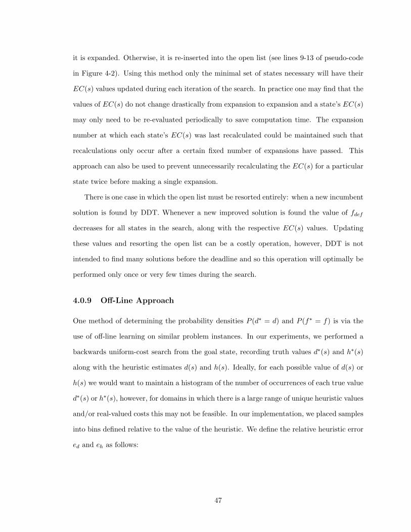
it is expanded. Otherwise, it is re-inserted into the open list (see lines 9-13 of pseudo-code
in Figure 4-2). Using this method only the minimal set of states necessary will have their
EC(s) values updated during each iteration of the search. In practice one may find that the
values of EC(s) do not change drastically from expansion to expansion and a state’s EC(s)
may only need to be re-evaluated periodically to save computation time. The expansion
number at which each state’s EC(s) was last recalculated could be maintained such that
recalculations only occur after a certain fixed number of expansions have passed. This
approach can also be used to prevent unnecessarily recalculating the EC(s) for a particular
state twice before making a single expansion.
There is one case in which the open list must be resorted entirely: when a new incumbent
solution is found by DDT. Whenever a new improved solution is found the value of fdef
decreases for all states in the search, along with the respective EC(s) values. Updating
these values and resorting the open list can be a costly operation, however, DDT is not
intended to find many solutions before the deadline and so this operation will optimally be
performed only once or very few times during the search.
4.0.9 Off-Line Approach
One method of determining the probability densities P (d∗ = d) and P (f∗ = f) is via the
use of off-line learning on similar problem instances. In our experiments, we performed a
backwards uniform-cost search from the goal state, recording truth values d∗(s) and h∗(s)
along with the heuristic estimates d(s) and h(s). Ideally, for each possible value of d(s) or
h(s) we would want to maintain a histogram of the number of occurrences of each true value
d∗(s) or h∗(s), however, for domains in which there is a large range of unique heuristic values
and/or real-valued costs this may not be feasible. In our implementation, we placed samples
into bins defined relative to the value of the heuristic. We define the relative heuristic error
ed and eh as follows:
47

ed =d(s)− d∗(s)
d∗(s)
eh =h(s)− h∗(s)
h∗(s)(4.5)
For example, given a pair d(s) = 15, d∗(s) = 20, we calculate the relative heuristic error
as ed = d(s)−d∗(s)d∗(s) = 15−20
20 = −0.25. In our experiments we divided the error into individual
bins of width 0.01. Once enough data has been collected the bins can be normalized for the
total number of samples taken and the resulting histogram can be used as
P (d∗ = d)/P (f∗ = f).
We used this method to collect relative heuristic error information for 20 instances of
2000x1200 Unit-Cost Four-Way Gridworld Navigation. The obstacles in these instances
were randomly assigned to each location with a probability of 0.35. The heuristic error
distributions (HED) are shown in Figure 4-3 for two individual instances and then for the
cumulative totals over all instances. In these plots, the Y-axis represents the value of h(s)
and the X-axis represents the relative error. One can see that for these uniformly random
instances the relative heuristic error is very condensed at the starting state, indicating that
most instances have a relatively similar solution cost. The heuristic error widens as the
partial solutions stretch across the search space until around h(s) = 2000, the width of the
grid world. From that point on, the relative heuristic error is bounded until states are very
close to solutions, at which point even small errors in the heuristic lead to large relative
values. Figure 4-4 illustrates slices taken from the cumulative HED for particular values
of h(s). By adding the state’s g(s) value to the values on the X-axis, these slices would
represent the density functions P (f∗ = f) used by DDT.
4.0.10 On-Line Approach
In this section we describe an approach that extends the single-step heuristic error model
from [15] to account for uncertainty in the heuristic estimates. Using this method the
cumulative distribution functions for d∗ and f∗ can be estimated on-line for any state s.
48
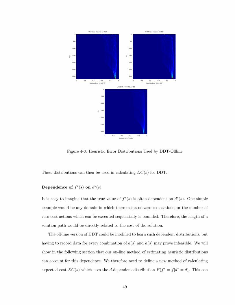
h(s)
Heuristic Error % (h-h*)/h*
Unit Grids - Instance 10 HED
0
500
1000
1500
2000
2500
3000
-1 -0.8 -0.6 -0.4 -0.2 0
h(s)
Heuristic Error % (h-h*)/h*
Unit Grids - Instance 13 HED
0
500
1000
1500
2000
2500
3000
-1 -0.8 -0.6 -0.4 -0.2 0
h(s)
Heuristic Error (h-h*)/h*
Unit Grids - Cumulative HED
0
500
1000
1500
2000
2500
3000
-1 -0.8 -0.6 -0.4 -0.2 0
Figure 4-3: Heuristic Error Distributions Used by DDT-Offline
These distributions can then be used in calculating EC(s) for DDT.
Dependence of f∗(s) on d∗(s)
It is easy to imagine that the true value of f∗(s) is often dependent on d∗(s). One simple
example would be any domain in which there exists no zero cost actions, or the number of
zero cost actions which can be executed sequentially is bounded. Therefore, the length of a
solution path would be directly related to the cost of the solution.
The off-line version of DDT could be modified to learn such dependent distributions, but
having to record data for every combination of d(s) and h(s) may prove infeasible. We will
show in the following section that our on-line method of estimating heuristic distributions
can account for this dependence. We therefore need to define a new method of calculating
expected cost EC(s) which uses the d-dependent distribution P (f∗ = f |d∗ = d). This can
49

0
0.2
0.4
0.6
0.8
1
150 200 250 300 350 400
Occ
urre
nces
h*
Unit Grids - HED (h=200)
0
0.5
1
1.5
2
600 800 1000 1200 1400 1600
Occ
urre
nces
h*
Unit Grids - HED (h=750)
0
0.5
1
1.5
2
2.5
1400 1600 1800 2000 2200 2400 2600 2800 3000
Occ
urre
nces
h*
Unit Grids - HED (h=1500)
Figure 4-4: Heuristic Error Distributions for Particular h(s) Used by DDT-Offline
be accomplished by first defining a d∗-dependent expected cost of a solution which assumes
the solution is reachable EC ′(s, d).
EC ′(s, d) =
∫ fdef
f=0[P (f∗ = f |d∗ = d) · f ]
+ P (f∗ > fdef |d∗ = d) · fdef (4.6)
We can then modify Equation 4.1 to account for individual possibilities of d∗(s) by
performing an integral rather than lumping them together into Pgoal.
EC(s) =
∫ dmax
d=0
[P (d∗ = d) · EC ′(s, d)
]
+ P (d∗ > dmax) · fdef (4.7)
50

Equation 4.7 can then be used in DDT, given a model which estimates P (d∗ = d) and
P (f∗ = f |d∗ = d).
Probabilistic Single-Step Error Model
The single-step error model, first introduced in [12] and then corrected and formalized in
[15], was designed as a method of calculating corrected heuristic estimates d(s) and h(s)
on-line by taking static (and possibly admissible) heuristics d(s) and h(s) and measuring
the single-step errors observed at each expansion in the search space. Given a state s, the
best child of that state bc(s) (the child with mininal f value), and the cost of transitioning
to bc(s), c(s, bc(s)), the single step errors in d(s) and h(s) are defined as follows:
ǫds = (1 + d(bc(s)))− d(s) (4.8)
ǫhs = (h(bc(s)) + c(s, bc(s)))− h(s) (4.9)
Given the mean single-step errors along an optimal path from a state s to the goal, ǫd
and ǫh, we can calculate d∗ and h∗ as follows:
d∗(s) =d(s)
1− ǫd(4.10)
h∗(s) = h(s) + d∗(s) · ǫh (4.11)
We extend this model by treating the single step errors along the optimal path from
s to the goal as independent identically distributed random variables with means µǫd , µǫh
and variances σ2ǫd, σ2
ǫh.
Calculating P (d∗ ≤ d) Because we have made the assumption that the individual single-
step errors ǫd are independent, we can apply the Central Limit Theorem and make the
claim that the mean ǫd of any sufficiently large number N of these errors is approximately
normally distributed with mean and variance calculated in Equations 4.12 and 4.13.
51
µǫd = µǫd (4.12)
σ2ǫd
=σ2ǫd
N(4.13)
Note that Equation 4.13 depends on the number of samples in the mean, N . When
using this mean in order to calculate d∗(s) using Equation 4.10, the number of samples of
single-step errors is equal to the number of steps between the state s and the best goal
under s: d∗(s) itself. While this value is clearly unknown, we can use the expected value of
d∗(s) for N by replacing ǫd with µǫd in Equation 4.10. Using Equation 4.12 to replace µǫd
with µǫd gives us Equation 4.14.
σ2ǫd
=σ2ǫd
d(s)1−µǫd
σ2ǫd
=σ2ǫd· (1− µǫd)
d(s)(4.14)
According to the Central Limit Theorem, as long as N is sufficiently large, these equa-
tions hold for both the mean of a set of one-step errors taken across the entire problem
space as well as any set taken across individual paths through that problem space. This
also holds regardless of the original distribution of ǫd(x), which is important because that
distribution is typically far from normal. See the top of Figure 4-5 for an example of the
distribution of ǫd(x) for the domain of 4-way Gridworld navigation using the Manhattan
Distance heuristic. In this domain, the one-step error ǫd(x) is equal to zero if the step was
taken in the direction of the Manhattan distance to the goal, or two if the step was taken in
the opposite direction. The overall probability of it being either zero or two depends on the
frequency of obstacles in the instance. Even with this very particular bi-modal distribution
the distribution of ǫd approaches normal very quickly. See Figure 4-5 for an example with
values of N = 10, 20, 40, 80, and 160.
Now that we have defined ǫd as a normally distributed random variable with mean
and variance defined by Equations 4.12 and 4.14, we can take Equation 4.10 and treat it
52

Figure 4-5: Central Limit Theorem Applied to 4-Way Gridworld One-Step Errors
as a function of a random variable in order to calculate the distribution functions for d∗.
Given that Equation 4.10 is differentiable and monotonically increasing for the valid range
of ǫd < 1, we can use the Cumulative Distribution Function technique in order to calculate
the CDF of d∗. The CDF technique is described in Figure 4-6.
Using this technique, with g(y) = (Equation 4.10) and therefore g−1(y) = y−d(s)y
, the
CDF of d∗ can be calculated in terms of the CDF of ǫd.
53
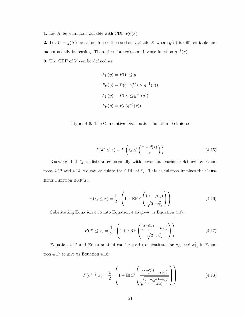
1. Let X be a random variable with CDF FX(x).
2. Let Y = g(X) be a function of the random variable X where g(x) is differentiable and
monotonically increasing. There therefore exists an inverse function g−1(x).
3. The CDF of Y can be defined as:
FY (y) = P (Y ≤ y)
FY (y) = P (g−1(Y ) ≤ g−1(y))
FY (y) = P (X ≤ g−1(y))
FY (y) = FX(g−1(y))
Figure 4-6: The Cumulative Distribution Function Technique
P (d∗ ≤ x) = P
(ǫd ≤
(x− d(s)
x
))(4.15)
Knowing that ǫd is distributed normally with mean and variance defined by Equa-
tions 4.12 and 4.14, we can calculate the CDF of ǫd. This calculation involves the Gauss
Error Function ERF(x).
P (ǫd ≤ x) =1
2·
1 + ERF
(x− µǫd)√
2 · σ2ǫd
(4.16)
Substituting Equation 4.16 into Equation 4.15 gives us Equation 4.17.
P (d∗ ≤ x) =1
2·
1 + ERF
(x−d(s)
x− µǫd)√
2 · σ2ǫd
(4.17)
Equation 4.12 and Equation 4.14 can be used to substitute for µǫd and σ2ǫd
in Equa-
tion 4.17 to give us Equation 4.18.
P (d∗ ≤ x) =1
2·
1 + ERF
(x−d(s)x− µǫd)√
2 ·σ2ǫd·(1−µǫd
)
d(s)
(4.18)
54
The key pieces of information necessary to use this equation are µǫd and σ2ǫd, the mean
and variance of the single-step errors along the path from a particular state s to the best
goal under s. Similar to the original model from [15], these values can be estimated by
tracking the mean and variance of the single-step errors observed so far either across the
entire problem space (Global Model) or along the partial solution leading up to state s
(Path Based Model).
Calculating P (f∗ ≤ f |d∗ = d) We can calculate the mean and variance of the normally
distributed mean single-step error ǫh similarly to equations 4.12 and 4.13.
µǫh = µǫh (4.19)
σ2ǫh
=σ2ǫg
N(4.20)
Again, N in this equation represents the number of single-step errors remaining along
the path from s to the goal and therefore the number of steps, d∗(s). Because we are
calculating the conditional distribution, we can assume that we are given a value for d∗(s).
Using the assumption that ǫh is normally distributed and Equation 4.11 we can then assume
that f∗(s) is distributed normally with the following mean and variance:
µf∗ = g(s) + h(s) + µǫh · d∗(s)
= g(s) + h(s) + µǫh · d∗(s) (4.21)
σ2f∗ = σ2
ǫh· (d∗(s))2
= σ2ǫh· (d∗(s)) (4.22)
Therefore, P (f∗ ≤ f |d∗ = d) will follow the standard for a normal distribution with
mean and variance defined by Equations 4.21 and 4.22. We can then use this distribution,
along with Equation 4.18 to calculate values of EC(s) using Equation 4.7.
55
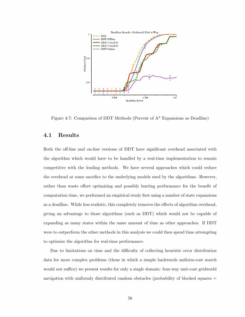
Figure 4-7: Comparison of DDT Methods (Percent of A* Expansions as Deadline)
4.1 Results
Both the off-line and on-line versions of DDT have significant overhead associated with
the algorithm which would have to be handled by a real-time implementation to remain
competitive with the leading methods. We have several approaches which could reduce
the overhead at some sacrifice to the underlying models used by the algorithms. However,
rather than waste effort optimizing and possibly hurting performance for the benefit of
computation time, we performed an empirical study first using a number of state expansions
as a deadline. While less realistic, this completely removes the effects of algorithm overhead,
giving an advantage to those algorithms (such as DDT) which would not be capable of
expanding as many states within the same amount of time as other approaches. If DDT
were to outperform the other methods in this analysis we could then spend time attempting
to optimize the algorithm for real-time performance.
Due to limitations on time and the difficulty of collecting heuristic error distribution
data for more complex problems (those in which a simple backwards uniform-cost search
would not suffice) we present results for only a single domain: four-way unit-cost gridworld
navigation with uniformly distributed random obstacles (probability of blocked squares =
56
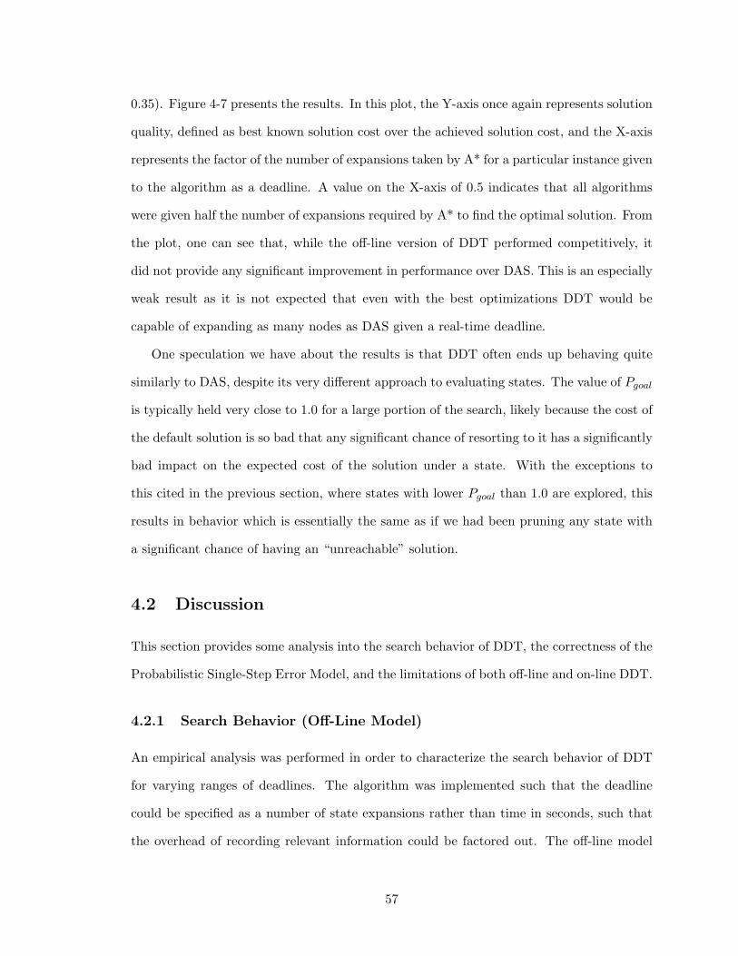
0.35). Figure 4-7 presents the results. In this plot, the Y-axis once again represents solution
quality, defined as best known solution cost over the achieved solution cost, and the X-axis
represents the factor of the number of expansions taken by A* for a particular instance given
to the algorithm as a deadline. A value on the X-axis of 0.5 indicates that all algorithms
were given half the number of expansions required by A* to find the optimal solution. From
the plot, one can see that, while the off-line version of DDT performed competitively, it
did not provide any significant improvement in performance over DAS. This is an especially
weak result as it is not expected that even with the best optimizations DDT would be
capable of expanding as many nodes as DAS given a real-time deadline.
One speculation we have about the results is that DDT often ends up behaving quite
similarly to DAS, despite its very different approach to evaluating states. The value of Pgoal
is typically held very close to 1.0 for a large portion of the search, likely because the cost of
the default solution is so bad that any significant chance of resorting to it has a significantly
bad impact on the expected cost of the solution under a state. With the exceptions to
this cited in the previous section, where states with lower Pgoal than 1.0 are explored, this
results in behavior which is essentially the same as if we had been pruning any state with
a significant chance of having an “unreachable” solution.
4.2 Discussion
This section provides some analysis into the search behavior of DDT, the correctness of the
Probabilistic Single-Step Error Model, and the limitations of both off-line and on-line DDT.
4.2.1 Search Behavior (Off-Line Model)
An empirical analysis was performed in order to characterize the search behavior of DDT
for varying ranges of deadlines. The algorithm was implemented such that the deadline
could be specified as a number of state expansions rather than time in seconds, such that
the overhead of recording relevant information could be factored out. The off-line model
57

0
2000
4000
6000
8000
10000
12000
01000020000300004000050000600007000080000
exp remaining
DDT: d(s) vs. dmax (Unit Grid 4-Way 2000x1200 p=0.35)
dmaxd(s)
1500
2000
2500
3000
3500
4000
01000020000300004000050000600007000080000
exp remaining
DDT: f(s) vs. EC(s)(Unit Grid 4-Way 2000x1200 p=0.35)
f(n)EC(s)
0
0.2
0.4
0.6
0.8
1
01000020000300004000050000600007000080000
prob
abili
ty
exp remaining
DDT: pgoal(Unit Grid 4-Way 2000x1200 p=0.35)
pgoal
Figure 4-8: Off-line DDT Search Behavior for Longer Deadline (13 A* Expands)
was applied to various instances of 4-Way Gridworld Navigation on a 2000x1200 size world
with uniformly distributed obstacles placed with a probability of 0.35 at each location.
Behavior for Longer Deadlines
The plots in Figure 4-8 show that for longer deadlines, similar to in DAS, the value of dmax
helps push the search towards finding a solution within the deadline. The deadline used in
this set is 100,000 expansions (as a reference A* took 373,730 expansions).
Unlike in DAS, the value of dmax does not act as a hard bound for which all states with
d(s) < dmax are judged equally. When the value of d(s) approaches dmax, the expected
cost EC(s) of the states selected for expansion will increase (as Pgoal decreases). In other
58
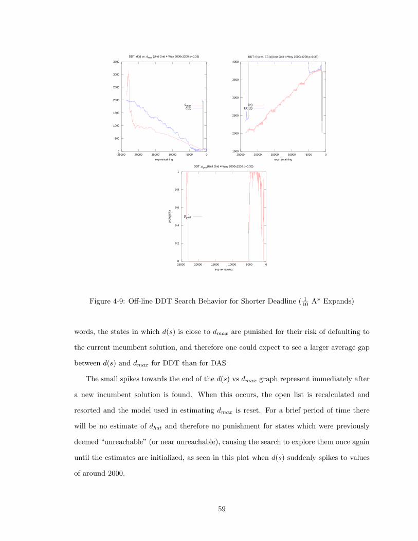
0
500
1000
1500
2000
2500
3000
3500
0500010000150002000025000
exp remaining
DDT: d(s) vs. dmax (Unit Grid 4-Way 2000x1200 p=0.35)
dmaxd(s)
1500
2000
2500
3000
3500
4000
0500010000150002000025000
exp remaining
DDT: f(s) vs. EC(s)(Unit Grid 4-Way 2000x1200 p=0.35)
f(n)EC(s)
0
0.2
0.4
0.6
0.8
1
0500010000150002000025000
prob
abili
ty
exp remaining
DDT: pgoal(Unit Grid 4-Way 2000x1200 p=0.35)
pgoal
Figure 4-9: Off-line DDT Search Behavior for Shorter Deadline ( 110 A* Expands)
words, the states in which d(s) is close to dmax are punished for their risk of defaulting to
the current incumbent solution, and therefore one could expect to see a larger average gap
between d(s) and dmax for DDT than for DAS.
The small spikes towards the end of the d(s) vs dmax graph represent immediately after
a new incumbent solution is found. When this occurs, the open list is recalculated and
resorted and the model used in estimating dmax is reset. For a brief period of time there
will be no estimate of dhat and therefore no punishment for states which were previously
deemed “unreachable” (or near unreachable), causing the search to explore them once again
until the estimates are initialized, as seen in this plot when d(s) suddenly spikes to values
of around 2000.
59

One can see from the plot of Pgoal over time that with a relatively long deadline DDT
does not perform much risky behavior early on in the search; expanding for the most part
states with Pgoal close to 1.0. We expect that this is due to the fact that the cost of the
incumbent solution from Speedier is so high that any significant chance of defaulting to it
results in that state’s EC(s) value to be increased significantly. Once a new incumbent so-
lution is found with significantly improved cost and the values of EC(s) have been updated,
the risk associated with not returning a new solution is far lower and therefore the search
will perform more risky behavior, expanding states with Pgoal < 1.0 (as can be seen from
the plot). This behavior seems like intuitive behavior when faced with a search problem and
a deadline. Until a decent solution is found, the agent should take fewer risks and ensure
that a solution better than the (high cost) default is found before the deadline arrives. Once
a decent solution is in hand there is then an opportunity for making more risky decisions
in the hopes of finding a more significant improvement.
Behavior for Shorter Deadlines
The plots in Figure 4-9 show a much different story than what occurred for longer deadlines.
The deadline used in this set is 36,000 expansions. As a reference, A* took 373,730 expands
to find the optimal solution. Looking at d(s) vs. dmax it is clear that the states being
explored are not considered “reachable” at all and their respective Pgoal values are zero.
When this is the case, the states in the open list all have fhat = fdef and the tie-breaking
strategy of minimal d(s) is being used in selecting states for expansion.
By choosing to break ties on low d(s), DDT has the property of devolving to Speedy
search (greedy on d(s)) for short deadlines. Looking at the d(s) vs. dmax plot, one can
imagine that during the early portion of the search when d(s) > dmax (and therefore Pgoal =
0) the DDT algorithm is performing a Speedy search. By performing the Speedy search
in the beginning when it was uncertain that the states were reachable at all within the
deadline, the algorithm catches up such that in the end there is a portion of the search
in which d(s) < dmax. For this last portion, the search actually does some consideration
60
of f(s) values and comes up with a better solution than the Speedy solution within the
deadline. This capability of speeding up the search when necessary and slowing down to
optimize cost once it is clear that there is time available seems like a natural and desirable
feature to expect for a deadline search algorithm such as DDT.
4.2.2 Verification of Probabilistic Single-Step Error Model
In order to validate the correctness of the Probabilistic Single-Step Error Model more di-
rectly than through empirical analysis of the on-line version of DDT, we performed a Monte-
Carlo analysis. A large number of trials were executed in which a sequence of single-step
errors was generated with known mean and variance. The distribution and values of the
errors were representative of a Four-Way Gridworld domain using the Manhattan Distance
heuristic. A starting value of d(s) was chosen and the corresponding d∗ values were calcu-
lated based on the sequences of errors. The empirical CDF was then calculated based on
the large distribution of recorded d∗ values. The analytical CDF of d∗(s) was calculated
using Equation 4.18, plugging in the known values of µd, σ2d, and d(s). The results of the
comparison are shown in Figure 4-10.
Overall, the analytical result proves to be an accurate estimation of the actual prob-
ability distribution for d∗. There was some amount of error in the model which is most
prevalent when the mean single-step error is closer to 1. In the case of four-way gridworld
this is most prevalent for smaller values of d(s) and a higher probability of experiencing the
single-step error. This can be seen in the plot for (p=0.35, d=30, N=10000) in Figure 4-10
(third row, left panel).
The error in the model can be attributed to the false assumption that the single-step
errors along the path from a state s to the goal are independent. While in the Monte Carlo
simulations the errors were sampled truly independently, their means were not distributed
normally as would be expected due to the Central Limit Theorem. This was most prevalent
for small values of d(s) and high probability of single-step errors. In Figure 4-11 the distri-
butions of ǫd are shown along with an attempted fit of a normal curve. The worst-fitting
61

curve fit is for the case of p=0.45, d=30. This error contradicts the assumption of normality
of this distribution necessary for Equation 4.16.
The problem with the assumption of independence is not with the way that the samples
are drawn, but with the method used to determine how many samples must be drawn. For
example, if ten samples were drawn independently and they happened to all have a value
of greater than one, then the path would not have reached a goal yet (d(s) would still be
greater than zero) and more samples would continue being drawn as steps are taken until
d(s) eventually reached zero. At this point the mean value of the one step errors would
be less than one, as expected. This clearly illustrates a dependence between one step error
values which invalidates the assumption of independence needed to apply the Central Limit
Theorem. For heuristics which have a lower probability of encountering single-step errors
or for larger values of d(s), the distribution of ǫd once again begins to resemble a normal
distribution and hence the resulting CDF for d∗(s) is more accurate. This can be seen in
Figure 4-11 by comparing the distributions as d(s) increases. It should also be noted that
in some domains it is very likely that the single-step errors will have some true dependence
between them. This possibility was not evaluated in this analysis and will likely introduce
additional error into the model.
4.2.3 Algorithm Limitations
Optimality for Large Deadlines
DAS has the beneficial feature of devolving to A* for larger deadlines when supplied with
an admissible heuristic, as it sorts the open list on uncorrected cost f(s). DDT does not
share this property, as both the off-line and on-line models sort the open list on expected
cost EC(s) which is far from an admissible heuristic. It is therefore expected that DDT will
not converge to optimal solutions as quickly as DAS, although empirical results show that
this was not the case for Gridworld Navigation. Contrastly, DDT has the beneficial feature
of devolving to Speedy for short deadlines, while DAS will resort to repeatedly pruning and
62

recovering states from the open list in a rather un-elegant manner.
Difficulty in Measuring Heuristic Error
The off-line model for DDT requires lookup tables for the distribution of d∗ and h∗ given a
particular state. We have presented one such method of measuring these distributions off-
line, but this method will not apply to any search space which is too large to be enumerated
using a backwards uniform-cost search. One would have to devise a more clever method
of measuring the error in the search space using an iterative deepening search, stochastic
measurements, or possibly limiting the search space in some other manner. Finding methods
which are feasible and produce realistic error models may prove to be difficult for some
domains.
Complexity and Algorithm Overhead
The empirical analysis presented in this thesis uses only the number of state expansions
as a deadline, in order to remove the effects of algorithm overhead. It is clear that both
the off-line and on-line models for DDT will produce a significant amount of overhead in
calculations of EC(s) and resorting the open list. There are several approaches which could
be taken to create an optimized version of DDT, such as using lookup tables for the Gaussian
Error Function or perhaps finding some simpler yet equivalent function which can be used
to sort the open list (such as what is done in Potential Search [14]). These obstacles would
have to be overcome before DDT could be used in a practical deadline search environment.
63
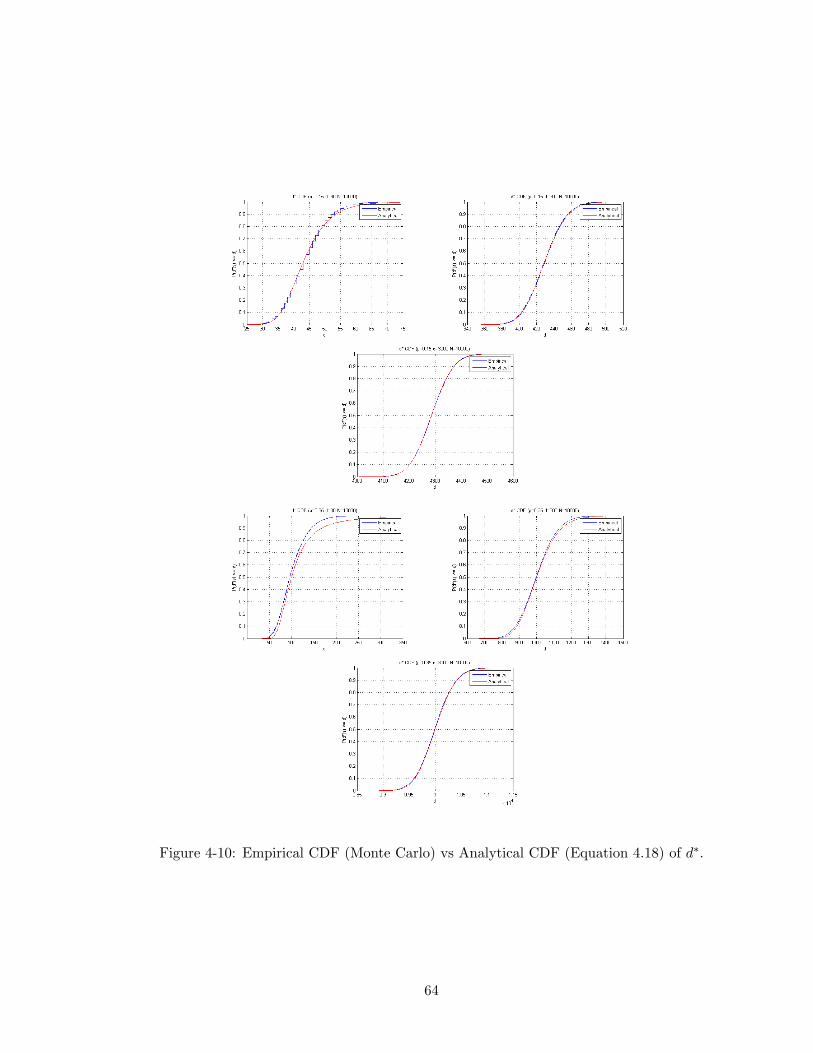
Figure 4-10: Empirical CDF (Monte Carlo) vs Analytical CDF (Equation 4.18) of d∗.
64
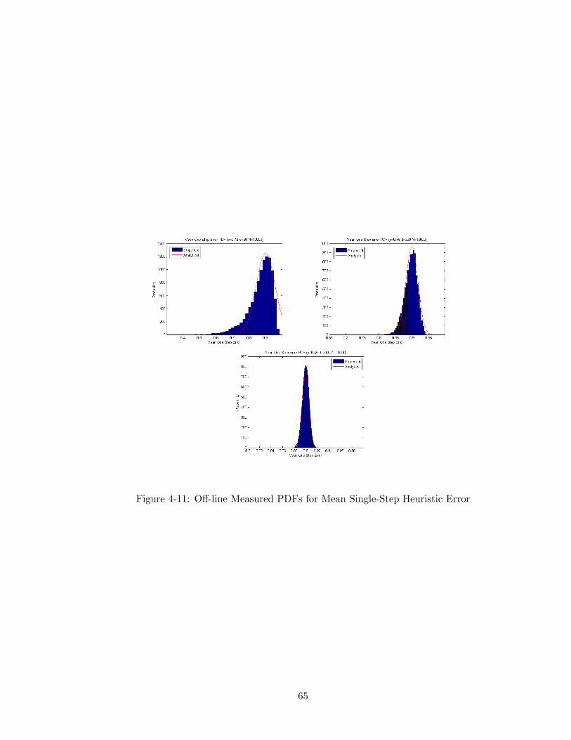
Figure 4-11: Off-line Measured PDFs for Mean Single-Step Heuristic Error
65

CHAPTER 5
CONCLUSIONS
5.1 Summary
The goal of this thesis was to develop new deadline-cognizant approaches for solving the
problem of heuristic search under deadlines that illustrate the possibility of improving upon
the current deadline-agnostic incumbent algorithms typically used. In this thesis, we pro-
posed two such algorithms: Deadline Aware Search (DAS) and Deadline Decision Theoretic
(DDT) search.
DAS is a simple approach that uses on-line measures of search behavior and a model
of heuristic error to dynamically determine which solutions are reachable within the time
remaining and pursue the best of those solutions. An empirical analysis was performed
comparing DAS to the leading incumbent anytime algorithm ARA*, as well as the most
recently proposed solution to deadline search, Contract Search, across a variety of domains
and deadlines. DAS was able to remain competitive in all domains and show a significant
improvement over both ARA* and Contract Search in several. DAS represents the first
general purpose deadline search algorithm to do so.
DDT is a more complex and principled approach that addresses the concept of risk
when searching under a deadline. Probability distribution functions for the true heuristic
values are learned either off-line through training or on-line through an extension of the
one-step error model used by DAS. Using these estimates, DDT attempts to minimize the
expected cost of the final solution returned before the deadline. A brief empirical analysis
was performed using a number of state expansions as a preliminary deadline method. The
66

results show that while off-line DDT could possibly be used as a competitive deadline search
algorithm, it does not improve the results obtained using DAS even with the additional
overhead required by the algorithm removed.
In working on DAS we have developed a new model that uses measurements of one-step
error in the heuristic values to calculate corrected inadmissible heuristics on-line. This model
was used in other work [15] on suboptimal search in which it was shown that the heuristics
learned via this method work significantly better for search guidance than other methods
of constructing corrected heuristics. It was also shown that by using this method on-line,
the corrected heuristics learn instance-specific information, something no other method has
demonstrated.
In working on DDT, the one-step error model was extended to construct new heuristic
functions which return probability density functions for the true distance-to-go and cost-
to-go. While this new probabilistic model did not perform well when used for DDT, we
believe that it holds potential for other applications which currently use simpler models of
uncertainty in heuristic error.
In summary, this thesis has introduced an algorithm which outperforms the state-of-
the-art approaches to deadline search, as well as other other new ideas which may find use
in further research into deadline search and search in general.
5.2 Possible Extensions
This section describes some of the possible directions in which the research started in this
thesis could be continued.
5.2.1 Additional Evaluation and Analysis
Restarting Weighted A* [11], described in the survey of anytime algorithms, does improve
on the results of ARA* in some of the domains which we used in our empirical analysis. It
would therefore be worthwhile to compare results from this algorithm with that of DAS.
67

Potential Search [14] is a recently proposed search method which expands states in order
of the probability of existing as part of a solution of a cost lower than a specific bound.
This algorithm can be used as an anytime algorithm, setting the bound at each iteration
to the cost of the solution returned from the previous iteration, finding the initial solution
using a Weighted A* search. Their results on a set of random 15-Puzzle instances improve
over their selected settings for Anytime Weighted A*. It would be interesting to include
this algorithm in the empirical analysis as well.
We chose to use the speedy solution as a default in our empirical analysis. This reprents
only one way to address the problem of dealing with failures to return solutions before the
deadline arrives. Other approaches, such as only considering the cost of solutions returned
and reporting the number of failures as a separate measure, may lead to more insight and
could be evaluated.
5.2.2 Correcting d(s) for DAS
DAS uses the path-based one-step error model for calculating corrected distance-to-go d(s),
used for pruning states that lead to unreachable solutions. [15] performed an in depth anal-
ysis of this new model for heuristic correction and found that it provides the best guidance
for suboptimal search out of the currently proposed methods for heuristic correction, how-
ever, it does not return the most accurate estimates of actual distance-to-go d∗(s). DAS
does not use the corrected heuristic for search guidance and may benefit from using one of
the other approaches that return more accurate estimates of true distance.
5.2.3 Estimating Reachability for DAS
Many different methods of defining “reachability” of solutions were presented in this thesis.
Expansion delay provided the most consistent performance in DAS and was therefore used
for the analysis of DAS and the implementation of DDT. There is no clear way of identifying
the use of expansion delay as the “correct” model of reachability, and there may exist a
better model that could improve performance. Both DAS and DDT depend substantially
68
on the estimate of dmax and it may represent the biggest opportunity for improvement if a
better model could be designed.
5.2.4 Recovering Pruned Nodes in DAS
The method of recovering pruned nodes in DAS used when all states have been deemed
unreachable was originally introduced as a quick fix which should have little impact on the
search in most cases. However, for very short deadlines, the estimates of dmax often end up
pruning all states from the search space and the method is invoked frequently. The method
currently designed does help return solutions in this cases of very short deadlines, but no
thorough evaluation was done against other possible methods. For example, as currently
implemented, the set of states recovered is selected such that the sum of their distance-to-
go values is less than the estimated number of expansions remaining in the search. This
selection does not at all account for the fact that the subtrees under each state are likely
much larger than d(s) and due to search vacillation many more than d(s) states are likely
to be explored in each subtree.
5.2.5 Further Evaluating Probabilistic One-Step Error Model
The extension to the one-step error model proposed for DDT that estimates probability
distributions for d∗(s) and f∗(s) proved not to work well when applied in DDT. Our Monte
Carlo analysis verified that the model used for d∗(s) was approximately correct given that
our assumptions about independance are met. We have not yet performed a similar analysis
for f∗(s). We believe that this new model of estimating heuristic error holds promise and
should be evaluated more thoroughly. Other algorithms use such probabilistic models of
heuristic error, such as Potential Search [14]. As currently proposed, Potential Search only
uses X and Y models for estimating distributions for the heuristic values. It is possible
that our probabilistic one step error model may provied a benefit over these more simple
approaches.
69

5.2.6 Modified Real-Time Search
Real Time Search interleaves planning and execution by performing iterations in which a
limited amount of search is performed in order to evaluate which next action to commit to
the current partial solution. These iterations are continued until a solution is found. This
addresses a different problem than contract search, but one can attempt to build on the
Real-Time Search approach and modify it to create a contract search algorithm.
The original proposed Real Time Search [7] suggested using a k-depth lookahead at
each iteration. DTA* [13] proposed a method of performing a variable amount of lookahead
that balances the cost of compution with the benefit of the reduction in solution cost due
to the additional search effort. To apply Real Time Search to the problem of searching
under a deadline, one would need to balance the amount of time spent performing each
iteration with the number of iterations necessary before a solution is found. This is a non-
trivial task, as for most domains the distance-to-go and therefore the expected number of
iterations required to a find a solution is not known with certainty. Even if one could predict
the necessary number of iterations, it is not immediately clear how the time remaining in
the search should be divided between the remaining iterations. Spending an equal amount
of time at each iteration may not be optimal, as one could consider that the impact of the
earlier decisions may have a more significant impact on the rest of the solution. While many
questions such as this would have to be addressed, the idea of extending Real Time Search
to address searching under a deadline seems like a possibility that should be evaluated.
70
BIBLIOGRAPHY
[1] Sandip Aine, P.P. Chakrabarti, and Rajeev Kumal. AWA* - a window constrained
anytime heuristic search algorithm. In Proceedings of IJCAI-07, 2007.
[2] Sandip Aine, P.P. Chakrabarti, and Rajeev Kumar. Heuristic search under contract.
Computational Intelligence, 26(4):386–419, 2010.
[3] Eric A. Hansen and Rong Zhou. Anytime heuristic search. Journal of Artificial Intel-
ligence Research, 28:267–297, 2007.
[4] Eric A. Hansen, Shlomo Zilberstein, and Victor A. Danilchenko. Anytime heuristic
search: First results. CMPSCI 97-50, University of Massachusetts, Amherst, September
1997.
[5] Peter E. Hart, Nils J. Nilsson, and Bertram Raphael. A formal basis for the heuristic
determination of minimum cost paths. IEEE Transactions of Systems Science and
Cybernetics, SSC-4(2):100–107, July 1968.
[6] Hironori Hiraishi, Hayato Ohwada, and Fumio Mizoguchi. Time-constrained heuristic
search for practical route finding. In Pacific Rim International Conference on Artificial
Intelligence, pages 389–398. Springer, 1998.
[7] Richard E. Korf. Real-time heuristic search. Artificial Intelligence, 42:189–211, 1990.
[8] Maxim Likhachev, Geoff Gordon, and Sebastian Thrun. ARA*: Anytime A* with prov-
able bounds on sub-optimality. In Proceedings of the Seventeenth Annual Conference
on Neural Information Porcessing Systems (NIPS-03), 2003.
71

[9] Judea Pearl. Heuristics: Intelligent Search Strategies for Computer Problem Solving.
Addison-Wesley, 1984.
[10] Ira Pohl. Heuristic search viewed as path finding in a graph. Artificial Intelligence,
1:193–204, 1970.
[11] Silvia Richter, Jordan Thayer, and Wheeler Ruml. The joy of forgetting: Faster any-
time search via restarting. In Symposium on Combinatorial Search, 2009.
[12] Wheeler Ruml and Minh B. Do. Best-first utility-guided search. In Proceedings of
IJCAI-07, pages 2378–2384, 2007.
[13] Stuart Russell and Eric Wefald. Do the Right Thing: Studies in Limited Rationality.
MIT Press, 1991.
[14] Roni Stern, Rami Puzis, and Ariel Felner. Potential search: a bounded-cost search
algorithm. In Proceedings of the Twenty-First International Conference on Automated
Planning and Scheduling (ICAPS-11), 2011.
[15] Jordan Thayer, Austin Dionne, and Wheeler Ruml. Learning inadmissible heuristics
during search. In Proceedings of the Twenty-First International Conference on Auto-
mated Planning and Scheduling (ICAPS-11), 2011.
[16] Jordan Thayer and Wheeler Ruml. Faster than weighted a*: An optimistic approach to
bounded suboptimal search. In Proceedings of the Sixteenth International Conference
on Automated Planning and Scheduling (ICAPS-08), 2008.
[17] Jordan Thayer and Wheeler Ruml. Anytime heuristic search: Frameworks and algo-
rithms. In SoCS 2010, July 2010.
[18] Jordan Thayer and Wheeler Ruml. Finding acceptable solutions faster using inad-
missible information. Technical Report 10-01, University of New Hampshire, April
2010.
72

[19] Jordan T. Thayer and Wheeler Ruml. Faster than weighted A*: An optimistic ap-
proach to bounded suboptimal search. In Proceedings of the Eighteenth International
Conference on Automated Planning and Scheduling (ICAPS-08), Fall 2008.
[20] Rong Zhou and Eric A. Hansen. Beam-stack search: Integrating backtracking with
beam search. In Proceedings of ICAPS-05, 2005.
73