Heuristics for finding a maximum number of disjoint bounded paths

Heuristics for Finding a Maximum Number of Disjoint Bounded Paths D. Ronen Department of Mathematics and Computer Science, Bar-llan University, Ramat Gan, Israel

Y. Per1 Department of Computer Science, Rutgers University, New Brunswick, New Jersey 08903 and Department of Mathematics and Computer Science, Bar-llan University, Ramat-Gam, Israel

We consider the following problem: Given an integer k and a network G with two distinct vertices s and t , find a maximum number of vertex disjoint paths from s to t of length bounded by k. In a recent work [ 91 it was shown that for length greater than four this problem is NP-hard. In this paper we present a polynomial heuristic algorithm for the problem for general length. The algorithm is proved t o give optimal solution for length less than five. Experiments show very good results for the algorithm.

I. INTRODUCTION

In the design of communication networks there is sometimes a requirement that the length of each communication path be bounded by some fixed number. The reason for such a requirement is the noise existing in communication lines. This noise increases with the length of the communication path.

We define a network as a graph C(V, E ) without multiple edges and self-loops. The length of a path is defined as the number of its edges. In this paper we consider the following problem: Given an integer k and a network G with two distinct vertices s and t , find a maximum number of vertex disjoint paths from s to r of length bounded by k.

In a recent work [9] it was shown that for length greater than four the above problem is NP-hard [7]. For length less than or equal to four, polynomial algorithms (using reductions to known polynomial problems like maximum matching or maximum flow) were given in [9].

It is interesting to note that for the related problem of finding a maximum number of disjoint paths of minimum total length, a polynomial algorithm is given by Surballe

In this article we present a polynomial heuristic algorithm for the above problem for general length. This algorithm incorporates distance considerations into maximum

W I .

NETWORKS, Vol. 14 (1984) 531-544 0 1984 John Wiley & Sons, Inc. CCC 002&3045/84/040531-14W.00

532 RONEN AND PERL

flow techniques. Such a similar incorporation was used by Dinic [2] (see also [4]) to decrease the complexity of maximum flow techniques. In Dinic’s algorithm the length of the augmenting path is bounded. However, in our problem we have to bound the length of each path constructed. Note that more efficient flow techniques, for example Karzanov [ 101 (see also [3]), Cherkasky [ l ] , Galil [6] , and Galil and Naamad [7] do not help here since we are interested in unit flow in the network.

In the next section a general description of the algorithm is given. It is composed of a procedure for finding an initial solution and an augmentation algorithm which will be described in Section 3. Section 3 also contains the complexity analysis of the algorithm. In Section 4 we prove that the algorithm gives an optimal solution for vertex disjoint paths bounded by length 4. As mentioned earlier, for higher length the problem is NP-hard. This proof is intended to provide a theoretical basis for the algorithm. Experiments showing very good results for the algorithm are presented in Section 5. Some of the proofs are long and are omitted. For the full proofs the reader is referred to [ l l ] .

2. GENERAL DESCRIPTION OF THE ALGORITHM

A k-bounded path is a path of length bounded by k. A solution for our problem is a set of disjoint k-bounded paths. An optimal solution is a solution containing such a set of maximum number of paths. The algorithm is combined of two phases.

Phase 1 : finding an initial solution Phase 2: repeated application of the augmentation algorithm, increasing each time

the number of paths in the solution by one until no such improvement is possible.

Finding an Initial Solution

There are several possible ways to obtain an initial solution. The most trivial of them is to start with an initial empty solution and apply immediately phase 2. How- ever, for efficiency we prefer to find an initial solution with the number of paths as large as possible.

A bounding solution is a solution such that no path of bounded length, disjoint to all the paths of the solution, exists in the network. In other words, the network obtained by removing the vertices of the bounding solution contains no k-bounded path. We choose to construct a bounding solution as an initial solution, according to the following algorithm.

PATHS. ALGORITHM FOR CONSTRUCTING A BOUNDING SOLUTION OF k-BOUNDED

Let G’ = G. While there exists a k-bounded path from s to t i n GI.

do; let d be the length of a shortest path from s to t i n G’.

Apply a breadth first search (BFS) to construct a subgraph G” of G’ containing these edges belonging to any path of length d from s to t in G’. Apply a maximum flow technique to find a set P(d) of maximum number of

MAXIMUM NUMBER OF DISJOINT BOUNDED PATHS 533

disjoint paths of length d from s to t in G”. Delete the vertices of the paths of P(d) from G’.

end;

The solution P is the union of all sets P ( d ) for all d < k. It is easy t o show that P i s a bounding solution of k-bounded paths. The complexity of finding the set P ( d ) of paths is O(l VI ”*IE 1) [ 9 ] . Thus the complexity of finding the bounding solution is

Phase 2 of the algorithm consists of repeated applications of the augmentation algo- O(klVJ”*1EI).

rithm described in the next section.

3. THE AUGMENTATION ALGORITHM

Before presenting the detailed description of the algorithm, we will explain the techniques used by the algorithm. Given a solution with f disjoint k-bounded paths, we will show how to improve the solution (if possible) and obtain f+ 1 k-bounded paths. A vertex is free if it is not contained in any path of the solution. The algorithm ap- plies a Depth First Search (DFS) starting from the vertex s and searching for the vertex t. The DFS prefers free vertices over nonfree vertices, such that the nonfree neighbors of a vertex are considered only after considering the free neighbors. In order to bound the path generated by the Depth First Search, every free vertex visited by the DFS is marked by its distance from s along the search path. A vertex may be visited by the DFS only if its present distance from s is less than the previous distance from s. Thus each free vertex is marked by the shortest distance from s obtained up to this stage of the DFS. Hence, the algorithm works according to the assumption (sometimes wrong) that if in the previous visit the search path failed to reach t i t will fail again when the search path at this stage is not shorter than the previous search path.

The DFS is performed as long as the last vertex in the search path has a free neighbor and as long as the search path to this neighbor is k-bounded. Such a neighbor is called a free reachable neighbor. If the search path reaches t ( t is always considered free), an improvement in the solution is achieved.

Assume a search path P1 = s, u(l), u(2), . . . , u(1) such that all free neighbors of u(l) were already considered.

Let P2 = s, w ( l ) , w(2), . . . , w ( j ) , . . . , w(m), r be a k-bounded path in the solution. Let w ( j ) be a neighbor of u ( l ) such that the distance of w ( j ) from t plus the distance of u ( l ) from s is less than k.

The algorithm performs a match between u(l) and w ( j ) and produces:

1. a new k-bounded path P1 = s, w ( l ) , u ( 2 ) , . . . , u(l), w ( j ) , w ( j + l ) , . . . , w(m),

2. a new search path P2 = s, w(l) , . . . , w ( j - 1). t and

The DFS will continue using the new search path P 2 . As stated, the DFS is performed using free vertices only. If the last vertex in the

search path does not have free reachable neighbors, a match will be done with one of the nonfree neighbors. It is possible t o perform a number of matches in a sequence. A

534 RONEN AND PERL

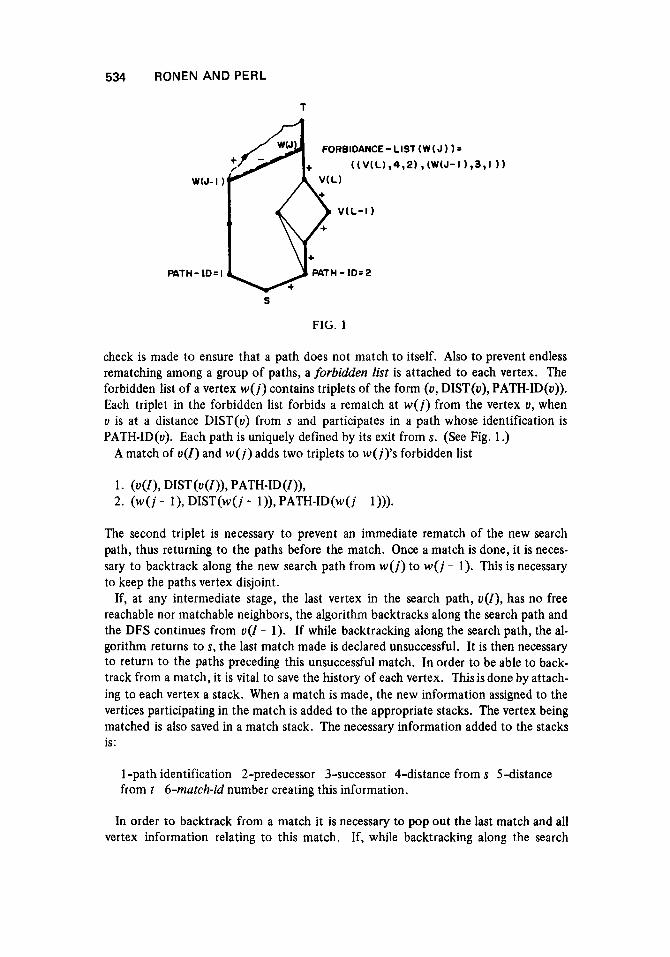
check is made to ensure that a path does not match to itself. Also to prevent endless rematching among a group of paths, a forbidden list is attached to each vertex. The forbidden list of a vertex w(j) contains triplets of the form (u, DIST(u), PATH-ID(u)). Each triplet in the forbidden list forbids a rematch at w(j) from the vertex u, when u is at a distance DIST(u) from s and participates in a path whose identification is PATH-ID(u). Each path is uniquely defined by its exit from s. (See Fig. 1 .)

A match of u(Z) and w(j) adds two triplets to w(j)’s forbidden list

1. ( ~ ( l ) , DIST(u(I)), PATH-ID(I)), 2. ( ~ ( j - l), DIST(w(j - l)), PATH-ID(w(j - 1))).

The second triplet is necessary to prevent an immediate rematch of the new search path, thus returning to the paths before the match. Once a match is done, it is necessary to backtrack along the new search path from w(j) to w ( j - 1). This is necessary to keep the paths vertex disjoint.

If, at any intermediate stage, the last vertex in the search path, u(Z) , has no free reachable nor matchable neighbors, the algorithm backtracks along the search path and the DFS continues from u ( l - 1). If while backtracking along the search path, the algorithm returns to s, the last match made is declared unsuccessful. It is then necessary to return to the paths preceding this unsuccessful match. In order to be able to backtrack from a match, it is vital to save the history of each vertex. Thisis done by attach- ing to each vertex a stack. When a match is made, the new information assigned to the vertices participating in the match is added to the appropriate stacks. The vertex being matched is also saved in a match stack. The necessary information added to the stacks is :

1 -path identification 2-predecessor 3-successor 4-distance from s 5-distance from t 6-match-id number creating this information.

In order to backtrack from a match it is necessary to pop out the last match and all vertex information relating to this match. If, while backtracking along the search


path, the algorithm returns to s and there is no match in the match stack, the algorithm simply exits s throughout another neighbor. All the free neighbors of s that were visited and marked by 1 will not participate in any search path. The algorithm ends when all free neighbors of s are marked by a distance of 1, and all nonfree neighbors contain s in their forbidden list.

THE ALGORITHM

initially assign DIST(u)+kt 1 for u = 1 , 2 , 3 ,..., IV1 DIST(s) + 0

let d = 0 be the depth of the match stack let P(d) be the given set of disjoint k-bounded paths.

V + S

DFS:

Condition (1): do; Ifthere is a free neighbor w of u marked by while DIST(u) < k

DIST(w) such that DIST(w) > DIST(u) t 1 then do; Add w to the search path.

Mark w by DIST(u) t 1.

Ifu = t then return. NOTE: a new path is found. u + w.

end;

else go to MATCH. NOTE: condition 1 is not satisfied for all free neighbors of u.

end;

Go to BACKTRACK ALONG SEARCH PATH. NOTE: the search path is not k-bounded.

MATCH:

Condition (2): if there is a nonfree neighbor w of u such that the triplet (u, DIST(u), PATH-ID(v)) is not in w’s forbidden list and such that DIST(u) t the distance of w from t < k then do; Let z be the predecessor of w. Add the triplet (v, dist(u),

path-id(u)) and the triplet (2 , dist (z), path-id(z)) to w’s forbidden list Store w in the match stack. Let d be the depth of the match stack. Perform a match between u and w thus obtaining a new set, P(d) of k-bounded paths. v+z . Go to DFS.

end;

536 RONEN AND PERL

BACKTRACK ALONG SEARCH PATH:

NOTE: at this stage v has no neighbors satisfying condition (1) or (2) . x + predecessor of u. Delete u from the search path. I f x # s t h e n d o ; v + x .

Go to DFS. end;

BACKTRACK FROM LAST MATCH:

NOTE: at this stage the algorithm has backtracked to s.

I f d > 0 then do; w + the vertex at the top of the match stack. u + predecessor of w. Let P(d) + P(d - 1). NOTE: return to the paths before the last match. Pop out w from match stack. Go to DFS.

end;

TERMINATE :

If s has a neighbor satisfying condition (1) or ( 2 ) then go to DFS, else terminate the algorithm with no improvement in the solution.

Time Complexity of the Algorithm

We calculate separately the time complexity of the DFS part and that of the matching part of the algorithm.

At the beginning of the DFS, all free vertices are marked by k + 1 as the bound for the distance from s. A visit to a free vertex is possible only if the present distance from s is less than the previous distance. It is therefore possible to scan the edges at most k times. Thus, the DFS will need at most O(klE1) time to find one more path.

In finding one more path, it is possible to perform a match at a vertex if the forbidden list allows it. The number of matches performed at a vertex is equal to half the number of the elements in the forbidden list. Each element is of the form (u, DIST(u), PATH-ID(u)). The number of neighbors of a vertex is DEGREE(v). Each such neighbor can be marked at most k times. Thus at most k different values of DIST(u) are possible. The number of disjoint paths possible in the network is certainly not more than 1V1. Thus PATH-ID may have at most different values. The number of matches possible is therefore SUM(DEGREE(u) kl V ( ) = k ( V1 SUM(DEGREE(v)) = kl VI ]El . Following the match, the algorithm assigns new values to the vertices participating in the new bounded path. There are at most k vertices in the bounded path, thus the matches performed require O(k2 11'1 ] E l ) time.

The time complexity for finding one more path is the sum of the time complexity for the DFS part and that of the matching part. It is therefore O(klE1 + k'l V ( ! E l ) =

In order to get the complexity of the algorithm we have to multiply the above complexity by the number of applications of the augmentation algorithm, which is bounded

O(k21 VI p1>.


by O( I Vl) since this is the maximum number of possible disjoint k-bounded paths in the network. Hence, the complexity of the algorithm is bounded by O(k21 “1’ \El ) .

However, in this analysis we did not use the fact that we first construct a bounding solution. If the maximum number of disjoint k-bounded paths in the network is q and p disjoint k-bounded paths are found in the bounding solution, then the complexity of the algorithm is bounded by O(k2q(q - p)lEl) . Note that the complexity of finding a bounding solution is O(kl VI’’21El).

The Space Complexity of the Algorithm

Because of the many matches and backtracks performed by the algorithm while searching for a new path, it is necessary to save the history of every vertex. A stack is assigned to each vertex. Whenever a change occurs to a vertex, the old information is pushed down into the stack and the new information is added at the top of the stack. When backtracking, this information is popped out of the stack and we are left with the previous information assigned to the vertex. Clearly the space requirement is lin- ear with the number of triplets in the forbidden lists and the depth of the stacks of all vertices.

As in the case of the time complexity, we shall distinguish between the space complexity of the DFS part and that of the matching part.

Every visit to a free vertex brings an allocation of one storage cell necessary to add the vertex to the search path. The number of possible visits to a vertex is k , thus the space complexity for scanning free vertices is ~ ( k l ~ l ) .

Each match requires the allocation of k storage cells in order to define the new k- bounded path. The number of matches is at most O(kl Vl \El) , thus the space complexity for performing matches is O(k2( V1 !El) . The total space complexity for finding one more bounded path is O(kl V1 t k21 VI 1E1) = O(k21 V1 IEI).

Once a path is found all storage structures (stacks, lists etc.) are initialized and thus this is the space complexity for finding any number of paths.

4. THEORETICAL BASIS FOR THE ALGORITHM

Theorem 1. All the paths found during the operation of the algorithm are vertex disjoint and k-bounded. The proof is technical and is omitted (see [ 111 ).

As is expected from the NP-hardness proof in [9] our algorithm does not necessarily provide optimal solution even for length five. For example see Figure 2 . Because the algorithm is quite complicated, it is difficult to prove a guaranty for the approxima- tion obtained, or any result about the probability of obtaining the optimum.

However, we shall prove in Theorem 2 that for length 4 the algorithm provides an optimal solution. This proof is intended to give some theoretical insight into the algorithm, though for length greater than four the solution obtained by the algorithm is not necessarily optimal. For length three the initial bounding solution is optimal (see [9]).

We will show that for a given network with fvertex disjoint 4-bounded paths, the algorithm will find ft 1 such paths iff is not the maximum number of vertex disjoint 4-bounded paths in the network. The symmetric difference of two sets A and B is (A - B) U ( B - A ) = A U B - A r7 B. For any set o f f + 1 such paths it is possible to obtain a symmetric difference with the set of the f given paths. The symmetric differ-

538 RONEN AND PERL

T

S

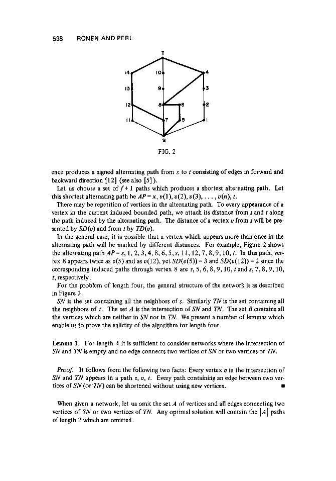
FIG. 2

ence produces a signed alternating path from s to t consisting of edges in forward and backward direction [12] (see also [S]).

Let us choose a set o f f + 1 paths which produces a shortest alternating path. Let this shortest alternating path be AP = x, u(l), u(2), u(3), . . . , u(n), t.

There may be repetition of vertices in the alternating path. To every appearance of a vertex in the current induced bounded path, we attach its distance from s and t along the path induced by the alternating path. The distance of a vertex u from swill be presented by SD(u) and from t by TD(u).

In the general case, it is possible that a vertex which appears more than once in the alternating path will be marked by different distances. For example, Figure 2 shows the alternatingpathAP=s, 1 , 2 , 3 , 4 , 8 , 6 , 5 , s , 1 1 , 12 ,7 ,8 ,9 ,10 , t . In thispath,vertex 8 appears twice as u ( 5 ) and as u(12), yet SD(u(5)) = 3 and SD(u(l2)) = 2 since the corresponding induced paths through vertex 8 are s, 5 ,6 ,8 ,9 ,10 , t and s, 7,8 ,9 ,10 , t, respectively.

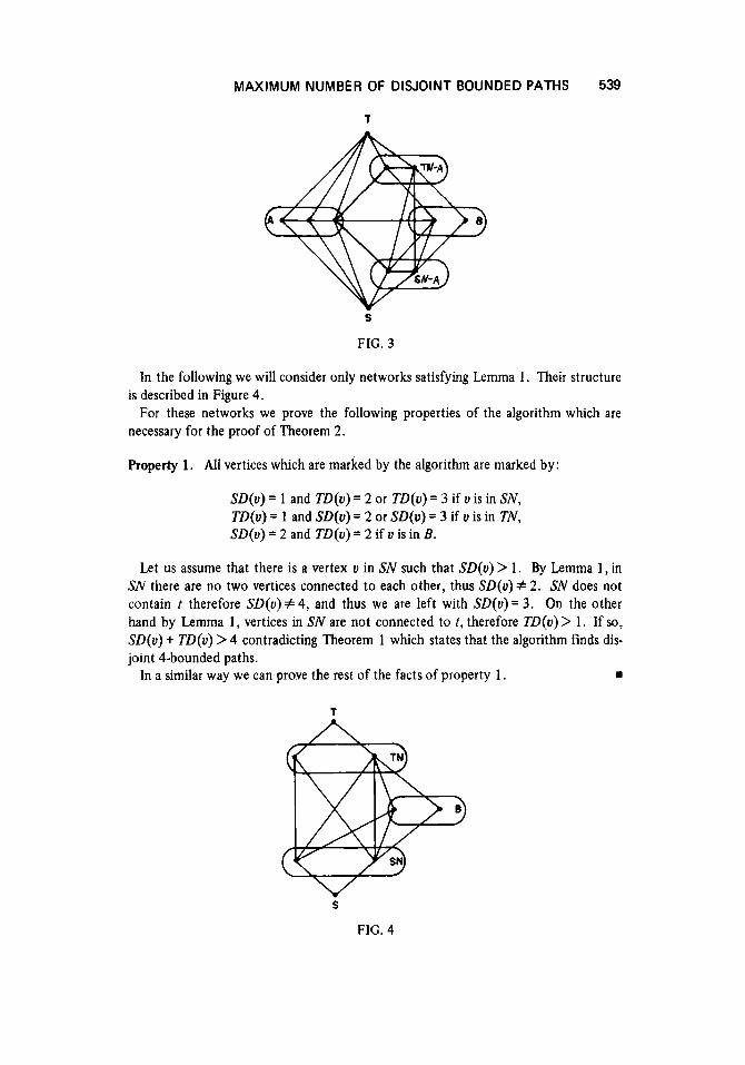
For the problem of length four, the general structure of the network is as described in Figure 3 .

SN is the set containing all the neighbors of s. Similarly TN is the set containing all the neighbors of t. The set A is the intersection of SN and TN. The set B contains all the vertices which are neither in SN nor in TN. We present a number of lemmas which enable us to prove the validity of the algorithm for length four.

Lemma 1 . For length 4 it is sufficient to consider networks where the intersection of SN and TN is empty and no edge connects two vertices of SN or two vertices of TN.

Proof: It follows from the following two facts: Every vertex u in the intersection of SN and TN appears in a path s, u, t. Every path containing an edge between two vertices of SN (or.TN) can be shortened without using new vertices.

When given a network, let us omit the set A of vertices and all edges connecting two vertices of SN or two vertices of TN. Any optimal solution will contain the \ A 1 paths of length 2 which are omitted.

MAXIMUM NUMBER OF DISJOINT

T

BOUNDED PATHS 539

S

FIG. 3

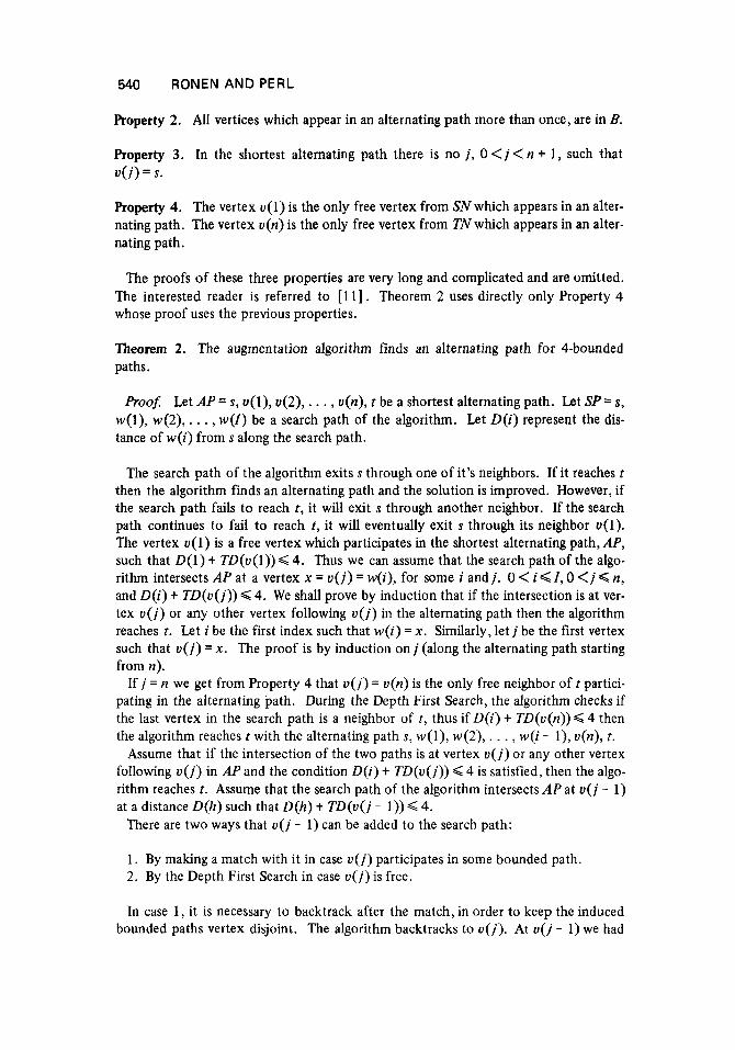
In the following we will consider only networks satisfying Lemma 1. Their structure

For these networks we prove the following properties of the algorithm which are is described in Figure 4.

necessary for the proof of Theorem 2.

Property 1. All vertices which are marked by the algorithm are marked by:

SD(u) = 1 and TD(u) = 2 or TD(u) = 3 if u is in SN, TD(u) = 1 and SD(u) = 2 or SD(u) = 3 if u is in TN, SD(u) = 2 and TD(u) = 2 if u is in B.

Let us assume that there is a vertex u in SN such that SD(u) > 1. By Lemma 1, in SN there are no two vertices connected t o each other, thus SD(u) # 2. SN does not contain r therefore SD(u) # 4, and thus we are left with SD(u)= 3. On the other hand by Lemma 1, vertices in SN are not connected t o t, therefore TD(u)> 1. If so, SD(u) t TD(u) > 4 contradicting Theorem 1 which states that the algorithm finds disjoint 4-bounded paths.

In a similar way we can prove the rest of the facts of property 1. m

T

S

FIG. 4

540 RONEN AND PERL

Property 2. All vertices which appear in an alternating path more than once, are in B.

Property 3. In the shortest alternating path there is no j , 0 < j < n t 1, such that u ( i ) = s.

Property 4. The vertex u(1) is the only free vertex from SN which appears in an alternating path. The vertex u(n) is the only free vertex from TN which appears in an alternating path.

The proofs of these three properties are very long and complicated and are omitted. The interested reader is referred to [ 1 11 . Theorem 2 uses directly only Property 4 whose proof uses the previous properties.

Theorem 2. The augmentation algorithm finds an alternating path for 4-bounded paths.

Proof: Let A P = s, u(l) , u(2) , . . . , u(n), c be a shortest alternating path. Let SP= s, w(l), w(2), . . . , w(Z) be a search path of the algorithm. Let D(i) represent the distance of w(i) from s along the search path.

The search path of the algorithm exits s through one of it’s neighbors. If it reaches c then the algorithm finds an alternating path and the solution is improved. However, if the search path fails to reach t, it will exit s through another neighbor. If the search path continues to fail to reach c, it will eventually exit s through its neighbor ~ ( 1 ) . The vertex u( 1) is a free vertex which participates in the shortest alternating path, AP, such that D(1) t TD(u(1)) < 4. Thus we can assume that the search path of the algorithm intersects AP at a vertex x = u ( j ) = w(i), for some i and j . 0 < i < Z, 0 < j < n, and D(i) t TD(u( j ) ) < 4. We shall prove by induction that if the intersection is at vertex u ( j ) or any other vertex following u ( j ) in the alternating path then the algorithm reaches c. Let i be the first index such that w(i) = x. Similarly, let j be the first vertex such that u ( j ) = x. The proof is by induction on j (along the alternating path starting from n).

If j = n we get from Property 4 that u ( j ) = u(n) is the only free neighbor o f t participating in the alternating path. During the Depth First Search, the algorithm checks if the last vertex in the search path is a neighbor of t, thus if D(i ) t TD(u(n)) < 4 then the algorithm reaches c with the alternating path s, w(l), w(2), . . . , w(i - l), u(n), c.

Assume that if the intersection of the two paths is at vertex u ( j ) or any other vertex following u ( j ) in APand the condition D(i ) t TD(u( j ) ) < 4 is satisfied, then the algorithm reaches c. Assume that the search path of the algorithm intersects AP at u ( j - 1) at a distance D(h) such that D(h) t TD(u( j - 1)) < 4.

There are two ways that u ( j - 1) can be added to the search path:

1. By making a match with it in case u ( j ) participates in some bounded path. 2 . By the Depth First Search in case u ( j ) is free.

In case 1, it is necessary to backtrack after the match, in order to keep the induced bounded paths vertex disjoint. The algorithm backtracks to u ( j ) . At u ( j - 1) we had


D(h) t TD(j - 1) < 4, thus at u ( j ) we get D ( i ) = D(h) - 1 and TD(u(j)) = TD(u(j - 1)) t 1 thus D(i ) t TD(u(j)) < 4. By the induction assumption we reach t .

In case 2, the algorithm adds u ( j - 1) to the search path during the DFS phase. The algorithm continues the DFS using one of the free neighbors of u ( j - 1). If after I steps we reach some vertex u(m), m > j , and D(1) t TD(u(m)) < 4 then by the induction assumption the algorithm finds an alternating path from s to t . If D(Ij t TD(u(m)) > 4 then the algorithm backtracks from u(rn), and u(m) is left free. The DFS continues with some other neighbor of u ( j - 1) and reach u ( j ) . At u ( j - 1) we had D(h) t TD(u(j - 1)) Q 4. Therefore at u ( j ) we get D(i ) = D(h) t 1 and T D ( u ( j ) = TD(u(j - 1)) - 1. Thus we get D(i ) t TD(u(j)) Q 4. Let us show that the algorithm is able t o reach u ( j ) . There are two ways that u ( j ) can be added to the search path:

1. By DFS in case u ( j ) is free. 2 . By making a match with it in case u ( j ) participates in some bounded path.

In case 1, u ( j ) is a free vertex. The algorithm checks that the present distance from s along the search path is less than the previous distance. The vertex u ( j ) is either marked by k t 1 (has never been visited), or it has been visited, but the condition D ( i ) t TD(u(j))<4 did not hold, or else by the induction assumption the search path of the algorithm would have reached t .

In case 2 , the vertex u ( j ) participates in some path. Since u ( j ) ’ s forbidden list does not contain u ( j - 1) we are able t o perform a match between w(i) and u ( j ) . Assume otherwise, that u ( j ) ’ s forbidden list contains a triplet of the form ( u ( j - 1) = w(i - 1 j, D(i - l), PATH-ID). The 4-bounded path induced by the match which creates this triplet is of the form s, w(l), w(2), . . . , u ( j - 11, u ( j ) , . . . , t . However, since w(1) uniquely identifies PATH-ID and the paths are 4-bounded, the path must be of the form s, w(l j, u ( j - I ) , u ( j ) , 1. By the induction assumption the algorithm should have reached t following this match, and no rematch is necessary. Hence u( j ) ’ s forbidden list does not contain u ( j - 1) and a match is possible at u ( j ) .

In both cases, once u ( j ) is reached and D ( i ) t TD(u( j ) ) < 4 holds, by the induction assumption we reach r.

5. EXPERIMENTAL RESULTS

In the experiment, we test networks with an initial bounding solution which is prob- ably not optimal. This possibility exists when the initial solution consists of fewer paths than the maximum number of disjoint paths (not necessarily k-bounded) in the network. The maximum number of disjoint paths in the network (without length constraint) is obtained by Dinic’s algorithm [2] .

In our experiment we choose random graphs consisting of 50 vertices and a varying number of edges. The edges are undirected (or more precisely, each undirected edge consists of two opposite directed edges). For each length and graph density a number of graphs are generated. From the random graphs generated, we choose only those for which the number of paths in the initial solution is less than the maximum number of paths without length constraints.

In these cases the augmentation algorithm is applied. We count the number of times an improvement is made on the initial solution. We also count the number of times

542 RONEN AND PERL

TABLE I

IEl = ~~

(VI = 50 200 400 600 800 1000 1500 2000 Total

k = 3 Graphs generated Graphs tested Improved solutions Sure optimal solutions

Graphs generated Graphs tested Improved solutions Sure optimal solutions


Graphs generated Graphs tested Improved solutions Sure optimal solutions Nonoptimal solutions




k = 4

k = 5

k = 6

k = 7

k = 8

Total

40 39 0

39

70 25

2 1

186 25 14 14

347 25 20 20

1

48 1 25 21 21

1

2422 21 21 21

3546 160 78 77

2

32 64 176 1088 25 25 25 23 0 0 0 0

7.5 25 25 23

193 567 315 25 10 5 23 10 4 23 10 4

95 8 10 10 10

17 2 2 2

I200 631 491 1088 62 35 30 23 35 10 4 0 35 10 4 0

96 1 6 0 6

96 1 6 0 0

1095 3456 6 149 0 0 6 149

1145 65 39 38

1144 35 24 24

364 27 22 22

1

48 1 25 21 21

1

2422 21 21 21

1095 9012 6 322 0 127 0 126

2

Fifth line for k = 6, k = 7 and total shows nonoptimal solutions.

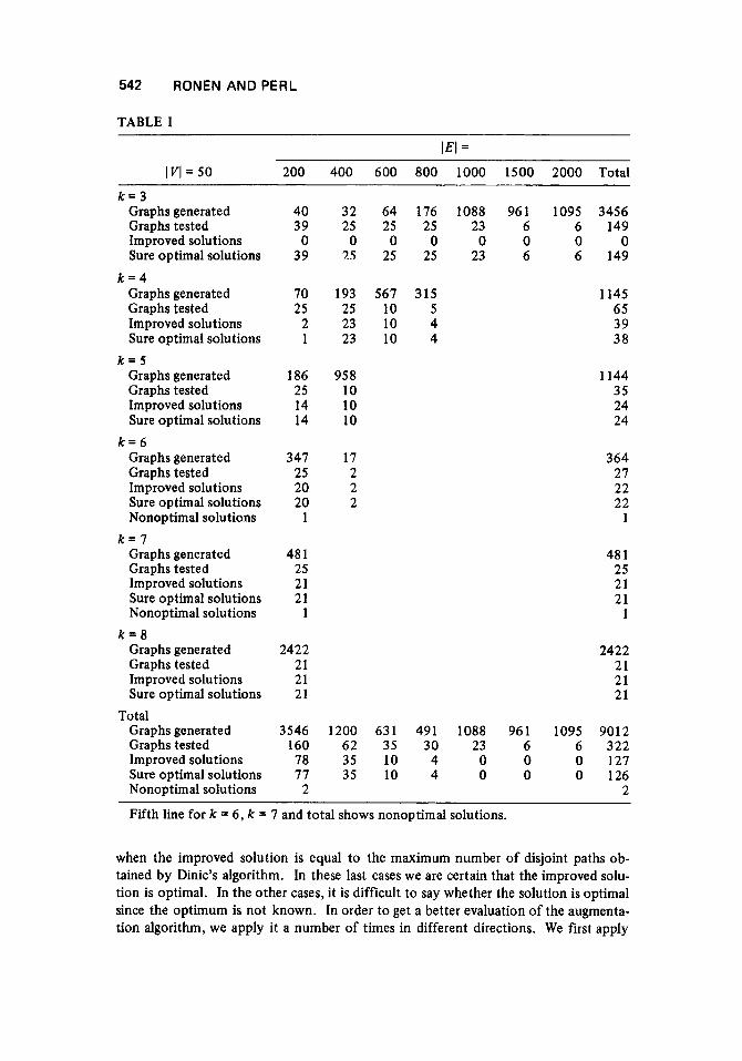
when the improved solution is equal to the maximum number of disjoint paths obtained by Dinic’s algorithm. In these last cases we are certain that the improved solution is optimal. In the other cases, it is difficult to say whether the solution is optimal since the optimum is not known. In order to get a better evaluation of the augmentation algorithm, we apply it a number of times in different directions. We first apply


the algorithm from s to t o n the network containing the initial solution. We apply the algorithm a second time from t t o s on the network containing the improved solution from the previous application. We then apply the algorithm a third time from s t o t starting with an initial empty solution and a fourth time from t to s on the solutionob- tained in the third time. Similarly, we exchange the role of s and t and apply the algorithm a fifth and sixth time from t to s and from s to t starting again with an initial empty solution. It is assumed that if the solution is not optimal, at least one such application will give a solution with more paths indicating a nonoptimal solution. The following table presents the experimental results.

Of the 9012 cases generated, the algorithm for the initial bounding solution is optimal in 8690 cases (96%). In the 322 other cases, the augmentation algorithm gives sure optimal solutions in 126 cases bringing the total sure optimal solutions to 98%. We find only two cases for which the augmentation algorithm certainly does not give an optimal solution. This occurs once for k = 6 and once for k = 7 when applying the augmentation algorithm back and forth from s to t and from t to s. Each application gives a different result. In view of all the tests that were performed we assume that the augmentation algorithm gives optimal solutions in all the other cases. There is no way to check this assumption in reasonable time.

From Table I we see that as the length increases, the initial solution is optimal in more cases. However, in the other cases, the augmentation algorithm also gives optimal solutions. In other words, when the length constraint is not severe, it is easy t o find an initial optimal solution because of the tendency of the algorithm for the initial solution to find shortest paths. This phenomenon also occurs when the graph density increases. It becomes more and more difficult to find an initial solution which is not optimal for large length and high density. In view of these results, we conclude that the algorithm is very good especially if it is applied back and forth in both directions.

References

[ 11 B. V. Cherkasky, Algorithm for construction of maximal flow in networks with complexity of O( V Z E '1') operations. Math. Methods of Solution of Economi- cal Problems (1 977) 11 7-1 25 (in Russian).

[ 21 E. A. Dinic, Algorithm for solution of a problem of maximum flow in a network with power estimations. Soviet Math. Dokl. 11 (1 970) 1277-1 280.

[ 3 ] S. Even, The max flow algorithm of Dinic and Kananov: An exposition. Infor- mation Technology, J . Moneta, Ed., North-Holland, Amsterdam (1 978) 233- 237.

[ 4 ] S. Even and R. E. Tarjan, Network flow and testing graph connectivity. SIAM J. Comput. 4 (1975) 507-518.

[6] I. T. Frisch, An algorithm for vertex-pair connectivity. Inter. J . Control 6

[ 6 ] Z . Galil, A new algorithm for the maximal flow problem. Proc. 19th Symp. on Foundations of Computer Science (1978) 23 1-245.

[ 71 M. R. Garry and D. S . Johnson, Computers and Intractability: A Guide to the Theory of NP-Completeness. Freeman, San Francisco (1 979).

(1967) 579-593.

This work was supported by a grant from the Israel Commission for Basic Research of the Israel Academy of the Science and Humanities and by a grant from the Re- search Authority, Bar-Ilan Univeristy, Ramat-Can, Israel.

544 RONEN AND PERL

[ 81 Z. Galil and A. Naamad, Network flow and generalized path compression. Proc. 11 th Annual ACM Symp. on Theory of Computing (1 979) 13-26.

[9] A. Itai, Y. Perl, and Y. Shiloah, The complexity of finding maximum disjoint paths with length constraints. Networks 12 (1982) 277-286.

[ 101 A. V. Karzanov, Determining the maximal flow in a network by the method of preflows. Soviet Math. Dokl. 15 (1 974) 434-437.

[ 111 D. Ronen, A heuristic algorithm for finding a maximum number of disjoint bounded paths in a network, M.Sc. thesis, Department of Mathematics and Com- puter Science, Bar-Ilan Univ., 198 1.

[ 121 J. W. Surballe, Disjoint paths in a network. Networks 4 (1974) 125-145.

Received December 12, 1983 Accepted February 9,1984

Documents

Heuristics for finding a maximum number of disjoint bounded paths