Embed Size (px)
Citation preview

Contents
1 Quickstart 41.1 Prerequisites . . . . . . . . . . . . . . . . . . . . . . . . . . . . . . . . . . . . 41.2 Walkthrough . . . . . . . . . . . . . . . . . . . . . . . . . . . . . . . . . . . . 4
Data Import . . . . . . . . . . . . . . . . . . . . . . . . . . . . . . . . . . . . 4Protein Mixture Filter . . . . . . . . . . . . . . . . . . . . . . . . . . . . . . . 6Parameter Settings . . . . . . . . . . . . . . . . . . . . . . . . . . . . . . . . 6Run Hexicon . . . . . . . . . . . . . . . . . . . . . . . . . . . . . . . . . . . 7
2 Hexicon Core 82.1 Prerequisites . . . . . . . . . . . . . . . . . . . . . . . . . . . . . . . . . . . . 82.2 Input Data . . . . . . . . . . . . . . . . . . . . . . . . . . . . . . . . . . . . . 8
LC-MS Maps . . . . . . . . . . . . . . . . . . . . . . . . . . . . . . . . . . . 8MS-MS Report . . . . . . . . . . . . . . . . . . . . . . . . . . . . . . . . . . 9Protein Sequences . . . . . . . . . . . . . . . . . . . . . . . . . . . . . . . . . 9Post Translational Modifications . . . . . . . . . . . . . . . . . . . . . . . . . 10
2.3 Filters . . . . . . . . . . . . . . . . . . . . . . . . . . . . . . . . . . . . . . . 12Background Protein Filter . . . . . . . . . . . . . . . . . . . . . . . . . . . . . 12
2.4 Parameters . . . . . . . . . . . . . . . . . . . . . . . . . . . . . . . . . . . . . 12Peptide / LC Settings . . . . . . . . . . . . . . . . . . . . . . . . . . . . . . . 12MS Settings . . . . . . . . . . . . . . . . . . . . . . . . . . . . . . . . . . . . 13Export Settings . . . . . . . . . . . . . . . . . . . . . . . . . . . . . . . . . . 13Advanced Settings . . . . . . . . . . . . . . . . . . . . . . . . . . . . . . . . 14Saving Parameters . . . . . . . . . . . . . . . . . . . . . . . . . . . . . . . . . 14
2.5 Other Customizations . . . . . . . . . . . . . . . . . . . . . . . . . . . . . . . 15Protease Specificity Scores . . . . . . . . . . . . . . . . . . . . . . . . . . . . 15
2.6 Running Hexicon 2 . . . . . . . . . . . . . . . . . . . . . . . . . . . . . . . . 15
3 Hexicon 2 Result Browser 163.1 User Interface . . . . . . . . . . . . . . . . . . . . . . . . . . . . . . . . . . . 163.2 File Handling . . . . . . . . . . . . . . . . . . . . . . . . . . . . . . . . . . . 16
File Loading . . . . . . . . . . . . . . . . . . . . . . . . . . . . . . . . . . . . 16File Unloading . . . . . . . . . . . . . . . . . . . . . . . . . . . . . . . . . . 17File Saving and Export . . . . . . . . . . . . . . . . . . . . . . . . . . . . . . 17
3.3 Dataset Navigation . . . . . . . . . . . . . . . . . . . . . . . . . . . . . . . . 17Selecting the Active Dataset . . . . . . . . . . . . . . . . . . . . . . . . . . . 17The Tree View . . . . . . . . . . . . . . . . . . . . . . . . . . . . . . . . . . . 17MDI Tabs . . . . . . . . . . . . . . . . . . . . . . . . . . . . . . . . . . . . . 18
3.4 Filtering and Processing . . . . . . . . . . . . . . . . . . . . . . . . . . . . . 183.5 Graphical Representations . . . . . . . . . . . . . . . . . . . . . . . . . . . . 19
Coverage Statistics . . . . . . . . . . . . . . . . . . . . . . . . . . . . . . . . 19Peptide Map View . . . . . . . . . . . . . . . . . . . . . . . . . . . . . . . . . 19Time Series View . . . . . . . . . . . . . . . . . . . . . . . . . . . . . . . . . 21
2

3.6 Graphics Export . . . . . . . . . . . . . . . . . . . . . . . . . . . . . . . . . . 22B-Factor Export . . . . . . . . . . . . . . . . . . . . . . . . . . . . . . . . . . 22
3

1 Quickstart
This section is for the impatient who want to see what Hexicon 2 does to their data. We shallassume that you have a complete and functional copy of Hexicon 2 binaries as well as the re-quired runtime libraries for your operating system (cf. section 2.1). Furthermore, you have alldata at hand, know your experimental parameters and all you want to do is get results – fast. Bewarned that some tinkering with parameter settings and downstream postprocessing are requiredfor optimal results.
1.1 Prerequisites
Hexicon 2 is a reference-based bottom-up workflow which can run using one reference LC-MSmap, at least one map of deuterated protein and the corresponding protein sequences. Moreformally, the files you need are:
• Reference dataset, one mzXML file per LC-MS map, line spectra
• Deuterated data, one mzXML file per LC-MS map (at least one), line spectra
• Protein sequence of your experimental construct
• Protein sequences of all significant other components in the mixture (if present)
While most parameter settings of Hexicon 2 are only needed for fine-tuning of the workflow, itis essential that you know some parameters concerning data acquisition. This includes:
• Instrument resolution (FWHM)
• Instrument calibration accuracy
• Retention time range during which peptides elute
1.2 Walkthrough
Data Import
Hexicon 2 opens with the data import window (Figure 1). Hit Add to load your LC-MS maps.After selecting a map in mzXML format, a dialog will pop up and ask you for incubation timeand group number. The group number is used to identify replicates: maps with the same incu-bation time and group number will be treated as experimental replicates. Enter 0 as incubationtime and group number of the reference.For subsequent deuterated datasets, enter the respective D2O incubation time in seconds andassign the same (arbitrary) group number to each set of replicate maps. The example in Fig-ure 1 shows two deuterated maps which consistute replicates of the 15 sec incubation time point,hence they belong to the same group.If you have an appropriately formatted MS/MS search report (cf. section 2.2), it is strongly rec-ommended that you provide Hexicon 2 with this information. A protein sequence in plain text
4

Figure 1: Hexicon 2 data import window.
format always needs to be specified. If you used a 100 % labeling control, e.g., by labeling indenaturing buffer, load that dataset and enter an arbitrary group number and time point higherthan for your longest-incubated actual sample. Check the box next to Use last time pointas 100% D reference. When the location of all datasets has been specified, proceed to theprotein mixture filter by clicking Next
Tip
For optimal performance, some tinkering with parameter settings may be required. For yourconvenience and for better reproducibility, the locations of the input files can be saved andrestored using Save and Open, respectively.
5

Protein Mixture Filter
This step is only required if your experiment contains nonnegligible amounts of more thanone protein. If this is not the case, proceed to the extraction parameters with Next.
Hexicon 2 is designed for the analysis of one protein of interest at a time. If other proteinsare present in the mixture at significant amounts (such that peptides originating from these pro-teins are detectable in the spectra), you need to provide their sequences as background set. Dothis with Add for each protein other than the protein of interest.The optional reference map which can be loaded at the bottom of this window is currently notused (build 12 JUN 2014) as it provided no measurable improvement of sensitvity in our testdata.
Parameter Settings
See section 2.4 for a detailed description of the available parameters. Only a few of these valuesmust be changed for Hexicon to produce useful data given that you are using a common LC-MSexperimental setup:
The Retention Time Range is crucial for sensitive feature extraction. It is highly discour-aged to run Hexicon on the entire map. Much better performance can be achieved by enteringthe time range at which your peptides elute from the chromatographic column. Make sure thatthe time window not only accomodates the reference peptides but also the deuterated ones anddo not worry about adding a minute or so at each side of the window.
An estimate of the actual instrument Resolution (FWHM) ( ± 10 %) is required for Hexi-con to get an estimate of the attainable mass precision. More importantly, if your detector tendsto drift over the course of an experiment, you should calibrate it regularly (at least before thefirst and after the last injection, to know which errors to expect) and record the mass deviation.Enter the largest relative mass deviation ( ∆mz
mz in ppm) that you expect for any of the analyzedmeasurements as Calibration Error (ppm).
Tip
If calibration logs are not available and you cannot reproduce calibration errors experimen-tally, have a look at the precursor mass values reported for MS/MS sequenced peptides andcompare them to theoretically expected masses. This corresponds to the delta M field ofMASCOT reports.
The Export Settings are intuitive and should be adjusted. In addition to the specified outputfile, Hexicon will create a number of other files in the same directory, including a runtime log(Hexicon.log) and a subdirectory (deuteration), in which measured deuteration distri-butions for each identified peptide are stored. Is is therefore recommended to use one dedicateddirectory for the result output of each Hexicon run.
6

Tip
Save parameter settings in the Hexicon result output directory for documentation and re-producibility. The resulting .hxpar file is a human-readable plain text file containing allparameter settings.
If all parameters are set, proceed to the Run tab with Next.
Run Hexicon
If no error message is displayed in the status monitor, start Hexicon with Start HexiconWorkflow. An approximate progress bar and the status monitor showing the contents of theHexicon.log file as it is created keep you informed about the progress and provide you withkey statistics. When the run has finished, a csv file containing one feature per line, as well as aYAML file will be created. The YAML file can be read by hxviewer, Hexicon’s result browser,which is the recommended way of postprocessing and viewing data.
7

2 Hexicon Core
This section describes the core of the Hexicon 2 workflow, upstream requirements, parametriza-tion, the structure of the output as well as recommendations for quality control and downstreamprocessing.
2.1 Prerequisites
You have most likely received Hexicon 2 binaries in a zipped folder. The archive contains theexecutables hexicon.exe and hxviever.exe, the libraries ms++.dll, hxcore.dll, sashimi.dll, yaml-cpp.dll, zlib.dll as well as Qt libraries (QtXml4.dll, QtSvg4.dll, QtGui4.dll, QtCore4.dll, image-formats/qsvg4.dll). The text file pepsintable.txt contains protease cleavage score definitions (cf.section 2.5).It may be necessary to install Microsoft Visual Studio 2010 runtime libraries available free ofcharge from Microsoft.
2.2 Input Data
LC-MS Maps
Hexicon 2 was designed for the analysis of high-resolution liquid chromatography mass spec-trometry data generated from high-resolution TOF or ion trap based instruments. Since theamount of data generated by such devices can be enormous and most of them provide sophisti-cated methods for peak picking, we leave this task to upstream processing by the user and startwith line spectra.The open mzXML format is currently the most widely used and most flexible open data formatfor mass spectrometry data. We are aware of the shortcomings of XML-based formats for datastorage and plan to provide support for other data formats as new open standards are emerging.In order to run Hexicon 2, you will need exactly one reference map containing undeuterated pep-tides, at least one map containing deuterated peptides, and the protein sequence of the constructused in your experiment.Hexicon 2 is geared towards the analysis of continuous labeling experiments, i.e., the massdifference over D2O incubation time is analyzed. Therefore, each LC-MS map needs one asso-ciated time point. Maps with the same time point and group number are treated as replicates, i.e.extracted deuteration values are averaged.Relative deuteration centroid values can be corrected for back-exchange using a 100 % deuter-ated control sample measured under identical LC-MS conditions. You can provide such mea-surements as a set of additional maps. Give these maps an arbitrary group number and timepoint that’s higher than the group numbers and time points of all other maps, then check the boxnext to Use last time point as 100% D reference.
8

MS-MS Report
Loading a MASCOT search report will greatly improve the quality of sequence assignment topeptides contained therein. Furthermore, it helps resolving ambiguous sequence assignments.The format is historically a copy of the peptide summary browser display, hence Hexicon 2 looksfor a whitespace or tab-separated file containing the following fields:
• Query ID
• Observed m/z
• Mr (measured)
• Mr (theoretical)
• delta m
• missed cleavages
• Ion Score
• E-value
• Rank
• Unique (letter U to denote uniqueness)
• Peptide sequence
Only the values printed in boldface are used, hence dummy values can be inserted in other fieldsto create Hexicon 2 compatible MASCOT reports. Sequences must be provided in the formatX.YYYYY.X with YYYYY being the peptide sequence. Residues flanking the cleavage site arenot used in the current release (12 JUN 2014), however this behavior may change. We are plan-ning on adding support for a simpler format for the specification of MS2 confirmed peptides inthe next release.
Protein Sequences
TheProtein Sequence field is mandatory. Load a plain text file containing the protein sequencecorresponding to your experimental construct in one-letter code. Only standard proteinogenicamino acids are allowed, however you may define some exotic amino acids as post translationalmodifications, given that they contain only C,H,2H,N,O,P,S and I atoms. Other atoms can likelybe included, however some elements, e.g., Selenium, throw NITPICK’s Averagine-based iso-tope pattern model off.It may be useful to add a Reference Sequence if you want to compare constructs of differentlength, containing mutations or just for the sake of using standardized sequence numbering. Po-sitions of found peptides will be mapped to their reference position (using ungapped sequence
9
alignment) and the reference sequence will be shown instead of the construct sequence whengenerating protein-level graphical output, i.e., peptide maps and coverage histograms. Note thatall graphical displays of Hexicon 2 will only allow comparing peptides of identical sequenceregardless of the reference sequence.
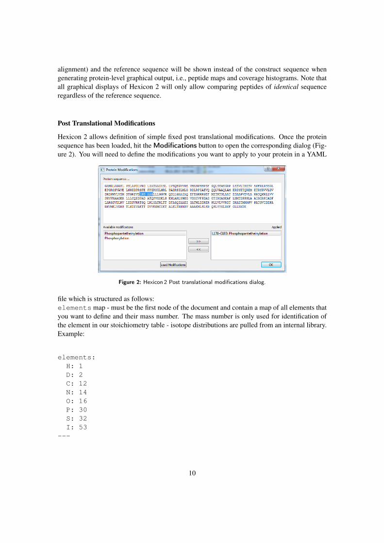
Post Translational Modifications
Hexicon 2 allows definition of simple fixed post translational modifications. Once the proteinsequence has been loaded, hit the Modifications button to open the corresponding dialog (Fig-ure 2). You will need to define the modifications you want to apply to your protein in a YAML
Figure 2: Hexicon 2 Post translational modifications dialog.
file which is structured as follows:elements map - must be the first node of the document and contain a map of all elements thatyou want to define and their mass number. The mass number is only used for identification ofthe element in our stoichiometry table - isotope distributions are pulled from an internal library.Example:
elements:H: 1D: 2C: 12N: 14O: 16P: 30S: 32I: 53
---
10

This block can be followed by any number of nodes, each containing following tags:modification: the name of the modification; short: a short identifier for display in thepeptide sequence; composition: a map of the elemental composition which will be added tothe modified amino acid’s stoichiometry (e.g., H: -2 means removal of two hydrogen atoms);applyTo: List containing one-letter code of amino acids to which the defined modificationcan be applied. Example:
modification: Phosphorylationshort: pcomposition:
H: 2O: 3P: 1
applyTo:- Y- S- T
---modification: Phosphopantetheinylationshort: pptcomposition:
H: 21O: 6P: 1C: 11N: 2S: 1
applyTo:- S
Once modifications have been loaded, use the mouse to highlight the parts of your protein se-quence which you want modified, pick the corresponding modification from the list of availablemodifications and hit >> to apply it.
Tip
Modifications can only include the elements listed in the above example since isotope pat-terns are only defined for these. Modifications with an elemental composition (more pre-cisely: isotope distribution) that strongly differs from the isotope pattern of a peptide con-taining only standard amino acids may not be correctly identified by our NITPICK featuredetection algorithm. If your modified peptide made it through feature detection, full model-ing of the isotope pattern is carried out in subsequent steps such that accuracy is no differentfrom unmodified peptides.
11

2.3 Filters
Background Protein Filter
Hexicon 2 can only analyze peptides corresponding to one protein at a time (referred to as proteinof interest). If your experiment contains other proteins (background proteins) in nonnegligibleamounts, there is a good chance of falsely assigning a sequence from the protein of interestto a peptide derived from a background protein. In order to avoid this, Hexicon 2 allows youto define the sequences of all background proteins in the filters tab. Import one plain text filefor each background protein in your experimental mixture. Peptides that match a backgroundsequence better than the protein of interest will be removed from the analysis after being usedfor internal mass calibration and false assignment estimation.In some cases, such filtering may be too strict and peptides of interest may be falsely assignedto background sequences. If this is the case, you can load a reference map in mzXML format,containing only the protein of interest measured under identical LC-MS conditions. Peptidesmatching a background sequence but found in the reference map will be rescued from the filter.Note: This feature has been disabled in the current release (12 JUN 2014) as it provided nomeasurable performance gain in our benchmarking studies.
2.4 Parameters
Hexicon 2 provides a number of customizable parameters which can be used to tune the sensi-tivity of the analysis and to adjust it to your experimental conditions.
Peptide / LC Settings
NITPICK feature detection is applied in a divide-and-conquer scheme: feature detection is car-ried out in each scan independently and detected features with similar mass in subsequent scansare merged. The fields Minimum / Maximum # Scans let you define in how many sub-sequent scans a peptide has has to be detected by NITPICK in order to be carried into furtheranalysis. The maximum scan number is rarely hit but if you have persisitent contaminationsconsistently detected by NITPICK, this will remove them. The Maximum Gap Time settingallows you to set a tolerance window in which a peptide need not be detected and still be mergedwith a previous peptide signal. It is advisable to increase this setting when you notice frag-mentation of your peptides, i.e., you get a large number of peptides with the same charge thatare detected in more than one contiguous region of the LC-MS map (another reason for this tohappen is too low mass precision tolerance in the FWHM setting).Hexicon 2 will try to assign peptide sequences to any detected feature regardless of MS2 identi-fication. For this purpose, exhaustive in-silico digestion is used to procude all peptides within agiven size range. Making the Peptide Length Range unnecessarily large will aversely affectruntime and sequence assignment specificity.
12

Tip
A good way to determine a suitable peptide length range for your experiment is to have alook at the peptides identified by MS2 or to do a discovery run with Hexicon 2 using a largerange (e.g. 5/45) and then to narrow down the range based on the results.
MS Settings
Since we are dealing with line spectra, there is no good way for Hexicon 2 to derive peak widthfrom input data. A good estimate of the scan Resolution (FWHM@400) is therefore requiredfor Hexicon 2 to estimate the attainable mass precision. A value of 40000 FWHM roughlytranslates to a precision of 6 ppm. Using this setting, features from subsequent scans with arelative mass difference ∆m/m of more than 6 ppm would be treated as two separate entities.The Calibration Error parameter represents the accuracy of your measurement, i.e., how muchmeasured mass deviates from actual mass and how much two measurements of the same peptideare allowed to differ in different maps. It is safe to set a fairly large value here since it is onlyused as worst-case value and empirically narrowed down during the analysis. If you feel thatsequence assignment or chromatogram alignment perform poorly, try altering this parameter in10 % intervals up or down.The Noise Quantile defines the peak intensity quantile that is safe to be considered as noise.It is used together with the SNR parameters (Advanced Settings) to pre-filter the spectrum. Ifyour data is heavily pre-filtered and no noise is present, set a very low value. Low values for thisparameter increase sensitivity, false discovery and mostly runtime.m/z Range and Charge State Range are self-explanatory. Having a charge state rangethat specificially matches your dataset will greatly accelerate feature detection and reduce falsepositive rates. We stronly recommend using Positive Ionization for all experiments. Negativeionization is incompatible with most current HDX protocols and was never tested in Hexicon.
Export Settings
There are several filters that you can apply for data export into the CSV file. The YAML filefor processing using hxviewer will not be filtered. Depending on your ionization settings, mostpeptides will produce more than one charge state which can be detected by Hexicon 2. Findingmultiple charge states with similar deuteration increases the confidence in data extraction. Itmay therefore be useful to discard results which have only one charge state, however it isnot recommended. For a quick discovery analysis, you may want to discard peptides with am-biguous sequence assignment. Such assignments occur when multiple theoretical peptidesequences match the extracted mass within the attainable mass precision. Hexicon 2 providesseveral means to resolve such sequence conflicts and to find the most likely correct assignment,hence discarding ambiguous assignments up front is discouraged. As there are currently nomeans to inspect individual replicates, we recomment discarding features with inconsistentreplicates. This filter will remove a peptide if the deuteration centroid standard deviation ex-ceeds a certain percentage of its absolute value. This centroid deviation cutoff is set to 20 %by default. If you get a very small number of results in the csv file but not in the YAML file, it
13

might be worth checking your filters and looking for a bad replicate.Hexicon lets you Separately Export deuteration distributions or a list of ambiguouspeptides. The deuteration distributions will be exported into a separate directory with one csvfile per feature. It will contain deuteration state abundance distributions for each replicate. Thelist of ambiguous peptides is a useful shortcut to defining peptides which you may want to havere-sequenced by MS2. Both the deuteration subdirectory and the list of ambiguous peptides willbe saved in the same directory as the main result list. This is also where the YAML file will besaved.
Advanced Settings
The first section deals with feature detection parameters. A running median will be computedfor each scan to define a background noise level. Each peak is then smoothed using a GaussianFilter and compared against the background noise. The width of this filter determines whetheryou emphasize local peaks or broad clusters to define which peaks lie above the noise level. Thetwo SNR parameters determine the intensity ratio of any raw (unsmoothed) peak over thebackground and its smoothed counterpart over the background required to pass the filter. Onlyif both smoothed and raw peak over background intensities exceed the set threshold values, thepeak is not treated as noise. These two SNR parameters are the main determinants of featuredetection sensitivity in Hexicon 2.The runtime of NITPICK increases quadratically with model size, hence Hexicon 2 attempts tofit models with independent (i.e., non-overlapping) isotope patterns separately. Busy spectra areoften highly overlapping and no split points can be found. In such cases, the Model Splitterparameter determines the number of models after which Hexicon 2 forces the model set to splitin order to keep runtime low. We do our best to stitch split models together in a sensitive waybut the fits are subobtimal at such breakpoints. If you notice that feature detection is choking,try reducing this setting. Better results are obtained with higher numbers here but significantslowdown of feature extraction was observed at about 200 models.The chromatogram alignment implemented in Hexicon 2 estimates two alignment toleranceterms based on the data and thereby already extends the search space for deuterated peptidesgenerously. If you feel, however, that alignment fails, you may try to manually extend thealignment window for deuterated peptides.
Tip
If you suspect that the chromatogram alignment is not doing a good job, try plotting ref-erence retention times versus retention times of deuterated peptides (both listed in the csvfile). Large scatter will usually indicate alignment problems.
Saving Parameters
Parameters are not automatically saved and cannot be retrieved once Hexicon 2 has started pro-cessing data! Please save your paramter settings file for reproducibility and convenience. We
14
recommend using one directory per Hexicon 2 analysis run where you can also store the settingsused to generated the results contained therein.
2.5 Other Customizations
Protease Specificity Scores
Hexicon 2 assigns cleavage scores based on cleavage probabilities empirically determined byHamuro and colleagues1. Table 2 of the corresponding publication was adapted (W-W cleavagewas not defined originally because the sequence WW had not been observed in the study) andreformatted to match a shape which can be read by Hexicon 2: In a whitespace-separated textfile, N fields of the first line define the one-letter amino acid alphabet A (typically 20 letters). Itfollows a N×N square matrix of nonnegative real-valued cleavage probabilities [0,1] where thevalue at position i, j (i denoting the row, j the column) stands for cleavage between A[j] (in P1)and A[i] (in P1′). Note the unconventional column-first notation which was kept for compliancewith Hamuro et al..Consider the following example file defining an arbitrary four-letter alphabet:
A C D E0.06 0.18 0.07 0.20.15 0.8 0.1 0.30.2 0.31 0.01 0
0.21 0.83 0.03 0.08
Examples for cleavage scores would be AAC∧DEACEDA (C/D): 0.31 or AACDEACED∧A (D/A):0.07. Internal peptides result from two cleavage events, hence a compound cleavage score mustbe found. Hexicon 2 assigns an internal peptide cleavage score
s =√s1s2
with s1 and s2 being the scores of the N- and C-terminal individual cleavage sites, respectively.Accordingly, the subsequence DEACED from the above example (denoted C.DEACED.A usingMASCOT convention) would receive a score of 0.15.Specificities are read from the plain text file "pepsintable.txt" which must be in the search path ofHexicon 2. In the Windows release, this would be the same direcory as the hexicon.exe binary.
2.6 Running Hexicon 2
Hexicon 2 will produce a log file that contains much useful information about the state of dataprocessing. The log file is shown in the Run tab of Hexicon 2 and saved in the directory of runoutput. Should Hexicon 2 quit unexpectedly without an error message, please have a look at thelog file which will contain debug output.
1Hamuro Y. et al., Rapid Commun Mass Spectrom. 2008; 22(7):1041-6
15

3 Hexicon 2 Result Browser
Hexicon 2 writes its results in YAML format which can be read by HXViewer, a graphical toolfor postprocessing and visualization of Hexicon 2 results.
3.1 User Interface
HXViewer has a split graphical user interface (GUI) which contains file and result managementin the left column and a multiple document interface (MDI) area for various tasks related to vi-sualization as well as interactive manipulation (Figure 3). Selecting the graphical representationof a peptide in any of the views will select and highlight the peptide in the tree view on the left.Modifications to either representation of the data will update the underlying model and affectany other data displays.
Figure 3: Hexicon 2 Result Browser User Interface
3.2 File Handling
File Loading
You can load one or more YAML files containing Hexicon 2 results by drag&drop from yourfilesystem browser into the tree view on the left, by clicking on the green + symbol above thatarea or by using the menu item File > Open. Since YAML is a text-based format, loading ofdata may take a while and happens in the background while you can start naming your datasets or
16

work on other, previously loaded data. Completely loaded datasets will appear in the dropdownmenu on the left from where you can select the active dataset to be displayed in the tree view.
File Unloading
Unload an opened dataset to free the memory it occupies by clicking on the red – button while itis active. This will only succeed if no other views (graphical displays) of that dataset are open.Note: Changes you made to the dataset will be lost unless you explicitly save it!
File Saving and Export
Your work is not saved unless you explicitly do so. Since HXViewer can only read YAML files,you should save your progress. We recommend saving to a new YAML file using the File >Save as menu item such that the original Hexicon 2 output is not lost. Peptides marked asdisabled will be saved as such and can be restored using HXViewer.Important: Only the active dataset (in the dropdown menu on the left - not the graphics view)will be saved. Make sure you save work in all your datasets before closing HXViewer.If you wish to create a csv file similar to the output originally generated by Hexicon 2, youcan use the menu item File > Export to csv. The dialog will ask you whether you wish tocreate a separate directory for deuteration files. Please note that answering Yes will create adeuteration directory in the same location as the exported csv file. If this happens to be thedirectory of the original Hexicon 2 output, it will be overwritten.
3.3 Dataset Navigation
Selecting the Active Dataset
Use the dropdown menu on the left to choose the active dataset. It will be displayed in the treeview below and all filters or visualizations will be applied to this dataset. You can change theactive dataset while there are still graphical displays of it, however interactive manipulation isonly possible to the active dataset. It is not required to save your work before changing theactive dataset.
The Tree View
The tree view on the left side of HXViewer presents rich information about the results of a Hexi-con 2 run. It groups the results by peptide and lists all peptides that were retrieved at least once ineach time point (i.e., have complete time series). Right-click the title bar to change how peptidesare sorted. The default is by position in the protein sequence. Expanding a peptide will showall found ions (charge states) which you can view in further detail by expanding. Ions displayedin red font have multiple sequence assignments which you can view by expanding their otherassignment(s) field. Right-click or double-click on the other assignment to jump to it in thetree view. Ions displaed in boldface are confirmed by MS2 sequencing. Peptides that contain atleast one ambiguous or confirmed sequence are displayed in red or bold, respectively.Double click on an ion to open a graphical display showing its deuterium incorporation over
17

time or on a peptide to show that display for all related ions. Other peptides or ions can be addedto the plot by dragging tree items and dropping them over an active plot. This can be done acrossdatasets.Right-click on an ion to disable it or on a peptide to disable all related ions. Disabled items willbe removed from any statistics or graphical displays, they will not be listed as sequence conflictsand not be exported to CSV. When saving the active dataset to a YAML file, disabled state ispreserved. Right-click on a disabled entitiy to re-enable it.
MDI Tabs
Graphical displays opened by a dataset will be grouped in one tab of the MDI area in the rightpart of the viewport. While this helps you keep your work structured, closing a tab provides aconvenient way of destroying all views on a dataset and thereby making it ready for unloading(unless there are open multi-dataset views open in other tabs).
3.4 Filtering and Processing
HXViewer provides two filter operations that we routine use as first-pass quality control: Fil-ter by intensity and Resolve sequence conflicts. If you plan on applying both filters, werecomment first applying the intensity filter and then proceeding to conflict resolution. Filterswill operate on the active dataset only. The intensity filter looks for ions with large deviation inintensity extracted from different maps. This is usually an indicator for either poor extraction insome datasets or for mis-alignment, i.e., assignment of a deuterated signal to a noncognate refer-ence ion. It has two passes: The filter will remove all features which exceed a relative intensitystandard deviation larger than the first cutoff set regardless of total intensity in the first pass. Thesecond pass removes all ions with a given standard deviation and an absolute intensity lowerthan a specfied quantile. This filter is of limited utility if you know that due to experimentalconditions, your samples show large variation in intensity.The conflict resolution filter inspects all ions with multiple sequence assignments and attemptsto determine, solely based on sequence, if any of the suggested sequences is more likely to becorrect than the others. It allows the user to specify residues after which cleavage is not al-lowed to occur. Furthermore, cleavage scores computed by Hexicon 2 can be compared. If onesequence is significantly more likely to be produced by the protease than another, it will be ac-cepted as correct sequence. Check the box next to Extend MS/MS to related ions if youwant MS2 confirmation of an ion also to be applied to related ions and thus all related sequencesto be preferred over any conflicting sequences.The Set all peptides menu contains two elements: Enable and Disable. This allows to (re-)setyour peptide selection quickly, e.g., if you want to consider only a small number of manuallyselected peptides. Please note that hxviewer does not have an undo function, hence you shouldsave your dataset to preserve the state of any manual processing you may have done prior toenabling or disabling all peptides.
18

3.5 Graphical Representations
Coverage Statistics
Activate the dataset of interest and choose the menu option Visualization > Coverage statis-tics to view a summary of general statistics about that dataset (Figure 4). Note that the recoverystatistics in this window do not match up with what is printed in the Hexicon 2 log file sincerecoveries in the log file do not check for presence of a unique sequence for a particular ion. Thehistogram in the upper part of the view shows the sequence assignment mass error. Since Hexi-con 2 performs internal mass-recalibration, the histogram should be zero-centered and its widthshould not exceed the attainable mass precision of your mass spectrometer. The bar plot in thebottom part of the view shows the number of features per backbone amide. It takes into accountthat the N-terminal amide back-exchanges rapidly under quench conditions and cannot be usedto extract HDX information. This figure is interactive and supports dragging as well as mousewheel zooming. Right-click on the figure to open the graphics export dialog (cf. section 3.6).
Figure 4: HXViewer Result Statistics View
Peptide Map View
The peptide map view can either display deuteration of all peptides in a single dataset (dynamicsmode, Figure 5) or compare deuteration differences between datasets (difference mode). Open
19

the peptide map view through the menu item Visualization > Peptide map. Choosing onlya reference dataset will open the dynamics view which shows deuterium incorporation of eachpeptide color-coded from blue (low) through green to red (high). The scale begins at zero andthe Dynamic Range parameter determines the upper limit of the scale. You can adjust thenumber of colors to obtain a more coarse or fine scale of color codings.Choosing two different datasets will open a deuteration difference view which shows the deuter-
Figure 5: HXViewer Peptide Map View
ation difference of the target dataset with respect to the reference on a blue-gray-red color scalerunning from the negative end of the dynamic range through zero to the positive end of thedynamic range. Deuteration differences between two peptides take into account the standarddeviation of deuterium incorporation into the two displayed peptides, hence peptides with largemeasurement uncertainty will appear less significantly blue or red than accurately measuredpeptides.Each box in the plot represents one peptide which may contain multiple charge states that arecombined to one compound deuteration value. Each box is split horizontally into a number ofsegments which correspond to D2O incubation time points. Therefore, the different colors in abox, bottom-up , indicate deuteration values or differences at each of the incubationtime points. A white diamond in a peptide box indicates MS2 confirmation of at least one ionrelated to that peptide.The peptide map view is interactive and supports drag and mousewheel zoom operations. Left-clicking a peptide will select the corresponding item in the tree view, right-clicking allows youto disable a peptide or to view its time series. If you are in difference mode, you will have theoption to disable either the reference, the target or both peptides. In this case, the time serieswill show both peptides’ deuterium incorporation over incubation time.Click the Secondary Structure icon to load a comma-separated secondaryi structure an-notation which can be displayed above the protein sequence. Hexicon 2 reads the following
20
representation of secondary structure: line 1: protein sequence; line 2: secondary structure overan alphabet of H, E, -; line 3: secondary structure prediction confidence on a scale of 0-9.Data in the third line is ignored in the current release (12 JUN 2014) of HXViewer.Click the Export icon to open the graphics export dialog (cf. section 3.6).
Time Series View
The time series view shows deuterium incorporation into one or more peptides over D2O incu-bation time. In order to open a time series view, double-click on an ion in the tree view. Doubleclicking on a peptide will display all ions associated with the sequence. Each time a new itemis added to the time series view, you will be asked to specify a color. When a peptide with mut-liple charge states is loaded, each charge state will be plotted as an individual line, the mediandeuteration will be plotted as separate bold line and the deuteration range spanned by all relatedions will be shaded.You can add further peptides to the time series view by dragging them from the tree view intothe plot area. HXViewer will try to construct a logical sequence from the peptides present in atime series view such that loading one peptide from a dataset will allow you to browse throughall peptides of that dataset using either the scrollbar below the plot area or the mouse wheelwhile over the plot area. When corresponding peptides from two or more datasets with identical(reference) sequence are loaded, HXViewer will let you scroll through all peptides present in alldatasets (intersection mode) or through all peptides present in any of the loaded datasets
(union mode) .
Click the distribution button to toggle the display of deuteration distribution estimates. Ifmultiple peptides are loaded, each peptide’s distribution will be plotted in a separate row.HXViewer will automatically estimate the required Y-axis range to accomodate all peptides inthe current view. The field Required #D range lets you override this setting such that theY-axis range will never be less than specified here. This may be useful if you want to get allplots in a series on the same scale.There are three modes of interacting with the data plotted in the time series view: In SelectionMode , you can click on peptides and charge states to select them in the plot and in the treeview. Selected peptides or charge states will be highlighted in blue and you can hit the Deletekey to disable the selected item. Right-clicking will open a context menu that lets you disable,select or remove the selected item. Please note the difference between disabling an item andremoving it from the plot: a disabled item will still be associated with the time series view andtherefore influences how the sequence of peptides is constructed. Removed items on the otherhand remain active but are no longer associated with the plot. The latter corresponds to reversingthe drag-and-drop operation from the tree view.In Marker Mode , clicking on a graph value will display the corresponding deuterationvalue. This value is transienly plotted and replotting, e.g., by scrolling back and forth in thesequence or by disabling/activating a charge state, will remove the label.Measurement Mode lets you measure deuteration difference between two different datapoints. Click on the first data point to initiate the measurement and click on a second point tocomplete it. You can abort a measurement by hitting Escape.
21

3.6 Graphics Export
Hexicon 2 has a standardized graphics export scheme. Export parameters can be set up in theexport dialog (Figure 6). Export into a PNG file guarantees that the current view will be saved as-is. Vector graphics can be obtained by exporting into PDF. Graphics exceeding the display widthcan be saved as multi-page PDF files whereas HXViewer ensures correct breakpoints. There isa bug in PDF export through Qt (Qt bug 23142, unresolved in Qt 4.x as of 2013/11/30) whichcauses Adobe PDF readers to misinterpret the colorspace information of graphics containingtransparency. This is invisible to physical printing and can be easily fixed by opening and re-saving the file in a vector graphics editor.
Figure 6: HXViewer File Export Dialog
B-Factor Export
Mapping of deuteration values or differences onto a crystal structure model is a popular way ofvisualizing HDX data. One commonly used way of encoding such information in a structure is toalter the B-Factors of a PDB file. PyMOL scripts like data2bfactor and color_b (http://pldserver1.biochem.queensu.ca/~rlc/work/pymol/, accessed 2013/12/04)can be used to modify and color-code B-Factors according to a text file. Use the menu itemVisu-alization > Create B-factor table to generate a text file compatible with the data2bfactorscript.As with the peptide map (section 3.5), you can choose between one or two datasets to createB-Factors from, to get B-factors corresponding to dynamics or difference output, respectively.The task of integrating information from multiple peptides for each amide is resolved as follows:for any amide, if MS2-confirmed peptides are available to cover this amide, use the longest ofthese. Otherwise, information from the longest MS-1 assigned peptide is used.
22

Tip
We are aware that there are multiple ways of mapping deuteration values from multipleoverlapping peptides onto each amide of a structure. While the presented approach consis-tently yielded the most faithful representation of our experimental data, this may not applyto other datasets. We are planning to include other deuteration export policies in furtherreleases. In the meantime you can take full control of what is exported with this "hack":Save your dataset first. Then disable all peptides using the Processing > Set all peptides> Disabled menu item (cf section 3.4). Open the peptide map view (section 3.5) and gothrough the peptide list (section 3.3) to activate only the peptides that you want exported.The peptide map will visually assist you identifying the correct peptides.
23