Mon. Not. R. Astron. Soc. 000, 1–15 (2010) Printed 25 October 2018 (MN LaTEX style file v2.2)

HI as a Probe of the Large Scale Structure in the Post-ReionizationUniverse

J. S. Bagla1, Nishikanta Khandai1,2, Kanan K. Datta1,3,41 Harish-Chandra Research Institute, Chhatnag Road, Jhunsi, Allahabad 211019, INDIA2 Department of Physics, Carnegie Mellon University, Pittsburgh, PA 15213, U.S.A.3 Department of Physics and Meteorology & Centre for Theoretical Studies, IIT, Kharagpur 721302, India4 The Oskar Klein Centre for Cosmoparticle Physics, Department of Astronomy, Stockholm University, Albanova, SE-10691 Stockholm, SwedenE-mail: jasjeet@hri.res.in, nkhandai@andrew.cmu.edu, kdatt@astro.su.se

25 October 2018

ABSTRACTWe model the distribution of neutral Hydrogen (HI hereafter) in the post-reionization universe.This model uses gravity only N-Body simulations and an ansatz to assign HI to dark matterhaloes that is consistent with observational constraints and theoretical models. We resolvethe smallest haloes that are likely to host HI in the simulations, care is also taken to ensurethat any errors due to the finite size of the simulation box are small. We then compute thesmoothed one point probability distribution function and the power spectrum of fluctuationsin HI. This is compared with other predictions that have been made using different techniques.We highlight the significantly high bias for the HI distribution at small scales. This aspect hasnot been discussed before. We then discuss the prospects for detection with the MWA, GMRTand the hypothetical MWA5000. The MWA5000 can detect visibility correlations at largeangular scales at all redshifts in the post-reionization era. The GMRT can detect visibilitycorrelations at lower redshifts, specifically there is a strong case for a survey at z ' 1.3. Wealso discuss prospects for direct detection of rare peaks in the HI distribution using the GMRT.We show that direct detection should be possible with an integration time that is comparableto, or even less than, the time required for a statistical detection. Specifically, it is possible tomake a statistical detection of the HI distribution by measuring the visibility correlation, and,direct detection of rare peaks in the HI distribution at z ' 1.3 with the GMRT in less than1000 hours of observations.

Key words: methods: N-Body simulations, cosmology: large scale structure of the universe,galaxies: evolution, radio-lines: galaxies

1 INTRODUCTION

Large scale structures in the universe are believed to have formedby gravitational amplification of small perturbations (Peebles 1980;Shandarin & Zeldovich 1989; Peacock 1999; Padmanabhan 2002;Bernardeau et al. 2002). Much of the matter in galaxies and clus-ters of galaxies is the so called dark matter that is believed to beweakly interacting and non-relativistic (Trimble 1987; Komatsu etal. 2009). Dark matter responds mainly to gravitational forces, andby virtue of larger density than baryonic matter, assembly of mat-ter into haloes and large scale structure is driven by gravitationalinstability of initial perturbations.

Galaxies are believed to form when gas in highly over-densehaloes cools and collapses to form stars in significant numbers(Hoyle 1953; Rees & Ostriker 1977; Silk 1977; Binney 1977).The formation of first stars (McKee & Ostriker 2007; Zinnecker& Yorke 2007; Bromm & Larson 2004) in turn leads to emission ofUV radiation that starts to ionize the inter-galactic medium (IGM).The period of transition of the IGM from a completely neutral to

a completely ionized state is known as the epoch of reionization(EoR), e.g., see Loeb & Barkana (2001). Observations indicate thatthe process of reionization was completed before z ∼ 6 (Fan, Car-illi, & Keating 2006; Becker et al. 2001; Fan et al. 2006). Many pos-sible sources of ionizing radiation have been considered, althoughstellar sources are believed to be the most plausible candidates, see,e.g., Bagla, Kulkarni, & Padmanabhan (2009).

Prior to the EoR, almost all the Hydrogen in the universe isin atomic form. Through the EoR Hydrogen is ionized till we areleft with almost no HI in the inter-galactic medium (IGM) and al-most all the HI resides in the inter stellar medium (ISM) of galax-ies. We focus on the post-reionization era in this work and our aimis to make predictions about the distribution of HI in this regime.It had been proposed by Sunyaev & Zeldovich (1972, 1975) thatthe hyperfine transition of Hydrogen may be used to probe primor-dial galaxies. This problem has been approached in past from theperspective of making specific predictions for existing instruments

c© 2010 RAS

arX

iv:0

908.

3796

v3 [

astr

o-ph

.CO

] 2

8 A

pr 2

010

2 Bagla, Khandai & Datta

like the Giant Meterwave Radio Telescope (GMRT)1 (Subrama-nian & Padmanabhan 1993; Kumar, Padmanabhan, & Subramanian1995; Bagla, Nath, & Padmanabhan 1997; Bagla 1999; Bharadwaj,Nath, & Sethi 2001; Bharadwaj & Sethi 2001; Bagla & White 2003;Bharadwaj & Srikant 2004; Bharadwaj & Ali 2005), or upcominginstruments like the the MWA2, ASKAP3 MeerKAT4 and SKA5,e.g., see Wyithe, Loeb, & Geil (2008). Much work in the last decadehas focused on making predictions for the power spectrum of fluc-tuations in HI, with an implicit assumption that it is easier to makea statistical detection than a direct detection. Further, it has beenargued that HI can be used as a tracer of the large scale structureand observations can be used to constrain cosmological parameterswith a special emphasis on observations of the baryon acoustic os-cillations (BAO) in the power spectrum (Visbal, Loeb, & Wyithe2008; Chang et al. 2008; Bharadwaj, Sethi, & Saini 2009). Most ofthe upcoming instruments are sensitive to the power spectrum offluctuations at large scales, certainly larger than the scale of non-linearity at the relevant epoch, and hence a significant fraction ofthe work done in terms of making predictions is based on lineartheory or approximations that work well in the linear and quasi-linear regime. The halo model has also been used for predicting thespectrum of fluctuations in the post-reionization universe (Wyitheet al. 2009; Wyithe & Brown 2009).

In this study we revisit the issue of predicting fluctuations anduse high resolution N-Body simulations. This allows us to studyfluctuations at scales comparable to, or even smaller than the scaleof non-linearity. We use dark matter simulations along with simpleansatz for assigning neutral Hydrogen in order to make predictionsof fluctuations in surface brightness temperature. Our model is dis-cussed in detail in §2 where we summarize our knowledge of the HIdistribution at high redshifts and motivate the assignment schemeswe use in this work . The N-Body simulations used by us are de-scribed in §2.1. Results of the HI signal are presented in §3. We thenmove on to review the relation between the source flux and observ-ables in radio interferometers, i.e. visibilities, in §4 and also discussthe sensitivity of interferometers. Finally we look at the prospectsof detection, both statistical and of rare peaks in §5. We concludewith a discussion in §6.

2 MODELING THE HI DISTRIBUTION

In this section we describe our model of the HI distribution at highredshifts. Our knowledge of the HI distribution in the universe isderived mainly from QSO absorption spectra, where the gas ab-sorbs in the Lyman-α transition of the Hydrogen atom. We knowfrom observations of these absorption spectra that much of theinter-galactic medium (IGM) is highly ionized and does not containa significant amount of neutral Hydrogen. Most of the neutral Hy-drogen resides in relatively rare damped Lyman-α systems (DLAS)(Wolfe, Gawiser, & Prochaska 2005). DLAS and other high columndensity absorption features are believed to arise due to gas within

1 See http://gmrt.ncra.tifr.res.in/ for further details.2 The Murchison Widefield Array (MWA). More details are available athttp://www.mwatelescope.org/3 The Australian Square Kilometer Array Pathfinder. Seehttp://www.atnf.csiro.au/projects/askap/ for details.4 The South African Square Kilometer Array Pathfinder. Seehttp://www.ska.ac.za/meerkat/overview.php for details.5 The Square Kilometer Array (SKA). See http://www.skatelescope.org/for details.

galaxies (Haehnelt, Steinmetz, & Rauch 2000; Gardner et al. 2001).It is possible to make a quantitative estimate of the total neutral Hy-drogen content in DLAS and study the evolution of the total neutralHydrogen content of the universe (Storrie-Lombardi, McMahon, &Irwin 1996; Rao & Turnshek 2000; Peroux et al. 2005). These ob-servations indicate that at 1 ≤ z ≤ 5, the neutral Hydrogen con-tent of the universe is almost constant with a density parameter ofΩHI ' 0.0016.

At low redshifts, the HI content can be estimated more di-rectly through emission in the Hyperfine transition. Observationsin the local universe indicate a much lower neutral Hydrogen con-tent than seen at z ≥ 1 (Zwaan et al. 2005). The neutral gas frac-tion in galaxies at intermediate redshifts appears to be much higherthan in galaxies in the local universe (Lah et al. 2007, 2009), i.e.,the neutral gas fraction in galaxies appears to increase rapidly withredshift z.

The spin temperature couples to the gas temperature throughcollisions of atoms with other atoms, electrons, ions and also theWouthuysen-Field effect (Purcell & Field 1956; Field 1958, 1959;Wouthuysen 1952a,b; Zygelman 2005; Furlanetto, Oh, & Briggs2006; Furlanetto & Furlanetto 2007a,b). Observations of 21 cm ab-sorption by DLAS indicate that the spin temperature is orders ofmagnitude higher than the temperature of the cosmic microwavebackground radiation (CMBR) at corresponding redshifts (Chen-galur & Kanekar 2000; Kanekar et al. 2009). This implies that theemission in the 21 cm hyperfine transition can be safely assumedto be proportional to the density of neutral Hydrogen, see, e.g.,Furlanetto, Oh, & Briggs (2006).

δTb(z) = 4.6 mK

(1− Tcmb

Ts

)(1 + z)2 H0

H(z)

× xHI (1 + δ)

[H(z)

(1 + z)(dv‖/dr‖)

]' 7.26mK(1 + z)2 H0

H(z)

MHI

1010M

(L

1Mpc

)−3

×[

H(z)

(1 + z)(dv‖/dr‖)

](1)

where xHI is the fraction of Hydrogen in neutral form, δ is thedensity contrast of the gas distribution, Tcmb is the temperature ofthe CMBR Ts is the spin temperature defined using the relativeoccupation of the two levels for the hyperfine transition:

n1

n0=g1

g0exp

−T?Ts

, (2)

where subscripts 1 and 0 correspond to the excited and ground statelevels of the hyperfine transition, T? = hν/kB = 68 mK is thetemperature corresponding to the transition energy, and (g1/g0) =3 is the ratio of the spin degeneracy factors of the levels.

Observations indicate that neutral gas is found only in galaxiesin the post reionization universe. We also know that at very low red-shifts galaxies in groups and clusters do not contain much neutralgas. As cold gas is associated with galaxies, we may assume thatit exists only in haloes that are more massive than the Jeans mass.Further, we may assume that neutral gas is predominantly foundin galaxies and not in larger haloes that may contain several largegalaxies. Jeans mass for haloes in a photo-ionizing UV background

6 These observational constraints are given as the ratio of the comovingdensity of neutral Hydrogen to the present day critical density. We adoptthe same convention here.

c© 2010 RAS, MNRAS 000, 1–15

HI in the Post-Reionization Universe 3

depends on the shape of the spectrum of the ionizing radiation, typ-ically we expect gas in haloes with a circular velocity in excess of60 km/s to cool, fragment and form stars. The mass within the virialradius is related to the circular velocity and the collapse redshift as:

Mvir ' 1010 M

(vcirc

60km/s

)3(1 + zc

4

)−3/2

(3)

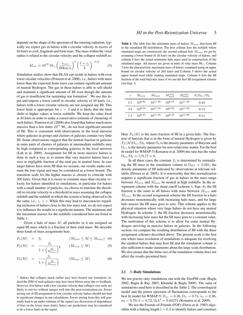
Simulation studies show that DLAS can reside in haloes with evenlower circular velocities (Pontzen et al. 2008), i.e., haloes with masslower than the expected Jeans mass can contain significant amountof neutral Hydrogen. The gas in these haloes is able to self shieldand maintain a significant amount of HI even though the amountof gas is insufficient for sustaining star formation7. We use this in-put and impose a lower cutoff in circular velocity of 30 km/s, i.e.,haloes with a lower circular velocity are not assigned any HI. Thislower limit is appropriate for z ∼ 3 and it is likely that the limitshifts to higher values at lower redshifts. We keep the value fixedat 30 km/s in order to make a conservative estimate of clustering ofsuch haloes. Pontzen et al. (2008) also found that haloes much moremassive than a few times 1011 M do not host significant amountof HI. This is consistent with observations in the local universewhere galaxies in groups and clusters of galaxies contain very littleHI. Some observations suggest that the neutral fraction in galaxiesin outer parts of clusters of galaxies at intermediate redshifts maybe high compared to corresponding galaxies in the local universe(Lah et al. 2009). Assignment for HI in more massive haloes isdone in such a way as to ensure that very massive haloes have azero or negligible fraction of the total gas in neutral form. In caselarger haloes have more HI than we assume, our results under esti-mate the true signal and may be considered as a lower bound. Thetransition scale for the higher masses is chosen to coincide with200 km/s. Given that it is easier to estimate mass than circular ve-locity for haloes identified in simulations, in particular for haloeswith a small number of particles, we choose to translate the thresh-old in circular velocity to a threshold in mass assuming the collapseredshift and the redshift at which the system is being observed to bethe same, i.e., zc = z. While this may lead to inaccuracies regard-ing inclusion of haloes close to the low mass end, we do not expectit to influence the results in a significant manner. The minimum andthe maximum masses for the redshifts considered here are listed inTable 1.

Given a halo of mass M , all particles in it are assigned anequal HI mass which is a fraction of their total mass. We describethree kinds of mass assignments here.

F1(M) = f1 (Mmin ≤M ≤Mmax) (4)

F2(M) =f2

1 +(

MMmax

)2 (Mmin ≤M) (5)

F3(M) =f3

1 +(

MMmax

) (Mmin ≤M) (6)

7 Haloes that collapse much earlier may have hosted star formation, in-deed the ISM of such galaxies may have been blown away due to feedback.However, few haloes with a low circular velocity that collapse very early arelikely to survive without merger well into the post-reionization era. Errorsarising out of HI assignment to low circular velocity haloes should not leadto significant changes in our calculations. Errors arising from this will gen-erally lead to an under estimate of the signal (see discussion of dependenceof bias on the lower mass limit), hence our predictions may be consideredto be a lower limit on the signal.

Table 1. The table lists the minimum mass of haloes Mmin that hosts HIin the simulated HI distribution. The first column lists the redshift wheresimulated maps are constructed, the second column lists Mmin we get byassuming a lower bound of 30 km/s on the circular velocity of haloes, andcolumn 4 lists the actual minimum halo mass used in construction of thesimulated maps. All masses are given in units of solar mass M. Column3 lists the characteristic maximum mass of haloes computed using an upperbound on circular velocity of 200 km/s and Column 5 shows the actualupper bound used while making simulated maps. Column 6 lists the HIfraction of the total baryonic mass if we use the first HI assignment scheme(see Eqn. 4.

z Mmin Mmax Msimmin Msim

max F1Ωnr/Ωb

5.1 108.83 1011.30 108.81 1011.30 0.24

3.4 109.04 1011.52 109.02 1011.50 0.15

1.3 109.43 1011.92 109.43 1011.90 0.11

Here Fk(M) is the mass fraction of HI in a given halo. The frac-tion of baryons that is in the form of neutral Hydrogen is given byFk(M)Ωnr/Ωb, where Ωb is the density parameter of Baryons andΩnr is the density parameter for non-relativistic matter. For the bestfit model for WMAP-5 (Komatsu et al. 2009) the ratio has the valueΩnr/Ωb ' 1/0.17 ' 6.

In all three cases the constant fk is determined by normaliz-ing the HI mass in the simulation volume to ΩHI = 0.001, thedensity parameter of HI indicated by observations at relevant red-shifts (Peroux et al. 2005). It is noteworthy that this normalizationrequires a significant fraction of gas in haloes in the mass rangebetween Mmin and Mmax be neutral at high redshifts. In the as-signment scheme with the sharp cutoff (scheme 1, Eqn. 4), the HIfraction is the same in all haloes with mass between Mmin andMmax. In the second assignment scheme the HI fraction in a halodecreases monotonically with increasing halo mass, and for largehalo masses the HI mass goes to zero. This scheme applies to thephysical situation where very large haloes do not have any neutralHydrogen. In scheme 3, the HI fraction decreases monotonicallywith increasing halo mass but the HI mass goes to a constant value.The motivation of this scheme is to allow for some neutral Hy-drogen surviving in massive haloes in galaxies. In the followingsection, we compare the resulting distribution of HI with the threeassignment schemes described above. The present work is the firstone where mass resolution of simulations is adequate for resolvingthe smallest haloes that may host HI and the simulation volume isalso sufficient to make statements about the large scale distribution.We also ensure that the finite size of the simulation volume does notaffect the results presented here.

2.1 N -Body Simulations

We use gravity only simulations run with the TreePM code (Bagla2002; Bagla & Ray 2003; Khandai & Bagla 2009). The suite ofsimulations used here is described in the Table 2. The cosmologicalmodel and the power spectrum of fluctuations corresponds to thebest fit model for WMAP-5: Ωnr = 0.26, ΩΛ = 0.74, ns = 0.96,σ8 = 0.79, h = 0.72, Ωbh

2 = 0.02273 (Komatsu et al. 2009).We use the Friends-of-Friends (FOF) (Davis et al. 1985) algo-

rithm with a linking length l = 0.2 to identify haloes and construct

c© 2010 RAS, MNRAS 000, 1–15

4 Bagla, Khandai & Datta

Table 2. Columns 1 and 2 list the size of the box and the number of particlesused in the simulations. Columns 3 and 4 give the mass and force resolutionof the simulations, while columns 5 and 6 tell us the redshift at which thesimulations were terminated and the redshifts for which the analysis weredone

Lbox Npart mpart ε zf zout(h−1Mpc) (h−1M) (h−1kpc)

23.04 5123 6.7× 106 1.35 5.0 5.04

51.20 5123 7× 107 3.00 3.0 3.34

76.80 5123 2.3× 108 4.50 1.0 1.33

a halo catalog. The HI assignment schemes are then used to obtainthe distribution of neutral Hydrogen.

Several existing and upcoming instruments can probe the post-reionization universe using redshifted HI emission. The GMRT canobserve redshifted HI emission from a few selected redshift win-dows whereas most other instruments have continuous coverage inredshift bounded on two sides. We choose to focus on the GMRTwindows, as these are representative of the range of redshifts inthe post-reionization universe. In particular we will focus on thefollowing redshift windows of GMRT: zout = 5.04, 3.34, 1.33.Finite box effects can lead to significant errors in the distributionof haloes that host galaxies, apart from errors in the abundance ofhaloes of different masses (Bagla & Prasad 2006; Bagla, Prasad,& Khandai 2009). The choice of simulations used in this workensures that such effects do not contribute significantly. Previousstudies have indicated that at z ' 0, we need a simulation boxwith Lbox ≥ 140 h−1Mpc for the finite size effects to be negligi-ble (Bagla & Ray 2005; Bagla & Prasad 2006). On the other handthe mass resolution of particles decreases as the cube of simulationvolume. We balance the requirements of high mass resolution and asufficiently large box size by using different simulations for study-ing the HI distribution at different redshifts. Details of the simula-tions are given in the table 2.

3 RESULTS

Given an HI mass assigment for particles in a simulation, we canproceed to compute the expected signal from the HI distribution bymaking mock radio maps and spectra. We also compute the powerspectrum in both the real and the redshift space. For redshift spacecalculations, we use the peculiar velocity information of particlesin haloes. Unlike earlier studies, we resolve haloes of individualgalaxies and hence the internal velocity dispersion is naturally ac-counted for and there is no need to add it by hand (Kumar, Padman-abhan, & Subramanian 1995; Bagla, Nath, & Padmanabhan 1997;Bagla & White 2003).

We use the clouds-in-cell (CIC) smoothing to interpolate den-sities from particle locations to grid points for the purpose of com-puting densities and the power spectrum. It is convenient to ex-press the HI power spectrum in terms of the brightness tempera-ture, though in comparisons with the dark matter power spectrumwe revert to the usual dimensionless form.

We define the real and redshift space scale dependant bias by

Figure 1. Effect of HI mass assignment type on bias. Solid,dashed and dot-dashed lines are for HI assignment types 1, 2 and 3 as described in eqs. 4-6.Bias is computed at z = 3.34 for the 51.2h−1Mpc box with Mmax =

1011.5M. .

the ratio of the corresponding dark matter and HI power spectra.

b(k) =

[PHI (k)

PDM (k)

]1/2

(7)

bs(k) =

[P s

HI(k)

P sDM

(k)

]1/2

(8)

We start by checking the effect of HI assignment scheme on theresulting distribution. We have computed the bias b(k) at z = 3.34for the Lbox = 51.2h−1Mpc simulation using the three schemesintroduced above. The results are shown in Figure 1 for the threeassignment types described in Eqs. (4-6). We see that at large scalesthe three assignment schemes give very similar results, whereasthere is some disagreement between the assigment scheme Eqn.(4)and the other two. The difference can be attributed to the fact thatthe scheme described in Eqn.(4) puts more HI mass in haloes withmasses near Mmax. The differences between the HI assignmentschemes are relatively minor. We choose to work with the schemedescribed in Eqn.(6) due to a better physical justification, as dis-cussed in §2. As mentioned before, if large mass haloes happen tohave a larger HI fraction than we assume then the signal will belarger than what we predict here.

It is noteworthy that while the bias is strongly scale dependentat large k (small scales), it flattens out to a constant value at smallk (large scales).

In order to check for the effects of a finite box size, we car-ried out a test for the 23 h−1Mpc simulation box. Instead of usingthe range of halo masses for HI assignment that is appropriate forz = 5.1, we work with a slightly smaller range so that haloes ofthese masses can be found in the 51.2 h−1Mpc simulation as well.Figure 2 shows the dark matter power spectrum (Top panel) and theHI power spectrum (Lower panel) with the HI assignment restrictedto a smaller range of masses, as described above. We see that thedark matter power spectra from the two simulations agree throughthe range of scales where there is an overlap. The HI power spec-

c© 2010 RAS, MNRAS 000, 1–15

HI in the Post-Reionization Universe 5

Figure 2. Top: The dark matter power spectrum in the simulations withLbox = 23 h−1Mpc and Lbox = 51.2 h−1Mpc at z = 5.1. The agree-ment in the two curves indicates that the finite box size effects do not lead toerrors in the smaller box at the redshift of interest. Bottom: HI power spec-trum in the same simulations, see text for details. Show the effect of finitebox size on the simulated HI power spectrum, good agreement between thetwo curves imples that the error is small.

tra also agree, though not as well as the dark matter power spec-tra. These differences are so small that we do not expect these toaffect the final results in a significant manner. The difference canbe attributed to the fact that clustering of haloes is affected morestrongly by the box size effects in simulations (Gelb & Bertschinger1994; Bagla & Ray 2005).

These tests validate our approach for assignment of HI tohaloes, and also show that the effects of a finite box-size are notsignificant at the level of the power spectrum or the mass function.

Figure 3. The power spectrum of fluctuations: the solid line shows the lin-early extrapolated power spectrum, the dashed line shows the non-lineardark matter power spectrum and the dot-dashed line shows the HI powerspectrum. All power spectra are for z = 3.34. The dark matter and theHI power spectra have been computed with the simulation with Lbox =51.2 h−1Mpc.

Figure 4. The dependance of bias on Mmin and Mmax. The solid curveshows b(k) for the values of Mmin and Mmax shown in Table 1. Thedashed line shows b(k) when we use the reference value for Mmax butincrease Mmin to twice the reference value. The dot-dashed curve showsb(k) whenMmax is chosen to be higher: 1011.9 M, whileMmin is keptat the reference alue. We see that as the characteristic mass of haloes withHI increases, b(k) increases. All curves are for z = 3.34 and have beencomputed with the simulation with Lbox = 51.2 h−1Mpc.

c© 2010 RAS, MNRAS 000, 1–15

6 Bagla, Khandai & Datta

Figure 5. This figure shows a scatter plot of δHI smoothed at a scale of3h−1Mpc with spherical top hat window, plotted as a function of δDMsmoothed at the same scale. The figure shows a random subset of pointsfrom the simulation with Lbox = 51.2 h−1Mpc at z = 3.34.

3.1 Bias

This is amongst the first studies of the HI distribution at high red-shifts where we resolve the smallest haloes that can host significantamount of HI while ensuring that the finite box size effects do notlead to an erronous distribution of haloes. One of the points thatwe can address here is the effect of non-linear clustering on the HIdistribution and the scale dependance of bias. Some of these effectsare illustrated in Figure 3 where we have plotted the power spec-trum of fluctuations: the solid line shows the linearly extrapolatedpower spectrum, the dashed line shows the non-linear dark matterpower spectrum and the dot-dashed line shows the HI power spec-trum. All power spectra are for z = 3.34. The dark matter andthe HI power spectra have been computed with the simulation withLbox = 51.2 h−1Mpc.

It is apparent that at k > 0.5 h Mpc−1 the effects of non-linearclustering significantly enhance the dark matter power spectrum. Atk ∼ 10 h Mpc−1, the enhancement is close to an order of magni-tude. This is of utmost interest for upcoming instruments that canresolve small angular scales.

We find that bias b(k) for the HI distribution is much greaterthan unity at high redshifts. This is to be expected of galaxies athigh redshifts (Fry 1996; Mo & White 1996; Bagla 1998a,b; Mo,Mao, & White 1999; Baugh et al. 1999; Magliocchetti et al. 2000;Benson et al. 2000; Roukema & Valls-Gabaud 2000; Sheth, Mo,& Tormen 2001; Wyithe & Brown 2009). We note that the bias isscale dependent, and leads to a larger enhancement in the powerspectrum at very small scales.

The value of bias depends strongly on the choice of the char-acteristic mass of haloes with HI. This is shown in Figure 4. Allcurves are for z = 3.34 and have been computed with the simula-tion with Lbox = 51.2 h−1Mpc. This figure illustrates that the biasat all scales varies monotonically with the charactersitic mass ofhaloes with HI. Variation is gentle at large scales but fairly strongat small scales. Therefore it is extremely important to have an accu-

rate estimate of the charactersitic masses of such haloes. Indeed, ithas been pointed out that observations of the amplitude of cluster-ing in the HI distribution can be used to constrain masses of haloesthat host DLAS (Wyithe 2008).

While the preceeding figures describe the statistical bias com-puted from the ratio of power spectra, Figure 5 shows the stochas-ticity of bias (Dekel & Lahav 1999) in the HI distribution. Thisfigure shows a scatter plot of δHI smoothed at a scale of 3 h−1Mpcwith a spherical top hat window, plotted as a function of δDMsmoothed at the same scale. The figure shows a random subset ofpoints from the simulation with Lbox = 51.2 h−1Mpc at z = 3.34.The scatter about the average trend in the δHI−δDM is significant,and increases as we go towards large overdensities in dark matter.The scatter becomes small if we smooth the density distribution atmuch larger scales.

Similar results concerning the effect of non-linear gravita-tional clustering and bias are obtained for other redshifts. We con-centrate on the evolution of bias and the power spectrum rather thango into a very detailed discussion of the HI distribution at each red-shift. We discuss simulated maps in the following subsection.

Figure 6 (left panel) shows the evolution of the redshift spacepower spectrum for the HI distribution. Curves show the ∆2

HI(k)as a function of k for z = 5.1 (solid line), z = 3.34 (dashedline) and z = 1.3 (dot-dashed line). Unlike the power spectrum inreal space, the enhancement at very small scales is less strong andthis is due to velocity dispersion within haloes at smaller scales.Power at larger scales is enhanced due to the Kaiser effect (Kaiser1987), leading to a relatively stronger enhancement at larger scales,hence the difference in shapes of the HI power spectrum in thereal space and the redshift space. Even though the amplitude ofdensity perturbations increases with time, we see that the amplitudeof brightness temperature fluctuations decreases instead. This is amanifestation of the decreasing correlation function for galaxies,see, e.g., Bagla (1998b); Roukema & Valls-Gabaud (1998).

The evolution of bias at large scales, denoted as blin(k) to em-phasise that it refers to scales where clustering is still in the linearregime, is shown in the right panel of Figure 6. We see that this de-creases from around 2.5 at z = 5.1 to 1.2 at z = 1.3, the variationis slightly steeper than (1 + z)1/2 and hence the gradual loweringof the amplitude of the brightness temperature power spectrum.

3.2 Radio Maps

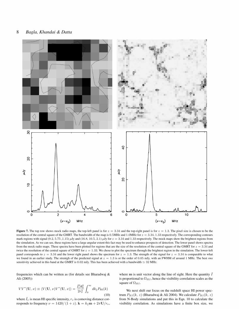
Figure 7 shows the simulated radio maps and spectra. The usualconversion from HI density to signal has been used for this (Furlan-etto, Oh, & Briggs 2006). The top row shows simulated radio maps,the top-left panel is for z = 3.34 and the top-right panel is forz = 1.3. The pixel size is chosen to be the same as the resolutionof the central square of the GMRT. The bandwidth of the map is0.5MHz and 1.0MHz for z = 3.34, 1.33 respectively. The corre-sponding contours mark regions with signal (9.2, 5.75, 1.15) µJyfor z = 3.34 and (16.8, 10.5, 2.1) µJy for z = 1.33. As we cansee in these maps, bright regions have a large angular extent. Thisfact may be used to enhance prospects of detection §5.

The lower panel shows spectra from the mock radio maps.These spectra have been plotted for regions that are the size of theresolution of the central square of the GMRT. We have chosen toplot the spectrum through the brightest region in the simulation.The lower-left panel corresponds to z = 3.34 and the lower rightpanel shows the spectrum for z = 1.3. The peak flux is around0.025 mJy and the FWHM of the line is close to 300 kHz. Thestrength of the signal for z = 3.34 is comparable to what we found

c© 2010 RAS, MNRAS 000, 1–15

HI in the Post-Reionization Universe 7

Figure 6. Left: Evolution of the HI powerspectrum ∆2HI

(k). Solid, dashed, dot-dashed lines are for redshifts z = 5.04, 3.34, 1.33 respectively. Right:Evolution of the HI linear bias.

in an earlier study, although the line width is much smaller. Thereason for a smaller line width is likely to be the supression of theHI fraction in very massive haloes. Considering the peak for whichthe spectrum has been plotted here, it may be possible to make a2σ detection with about 2 × 103 hours of observations with thecentral square of the GMRT (§5). Given that the GMRT observes amuch larger volume at these redshifts that the simulation volume,it is highly likely that even rarer peaks in the HI distribution willbe observed in a generic pointing (Subramanian & Padmanabhan1993).

The strentgh of the predicted signal at z = 1.3 is of the orderof 0.05 mJy, with an FWHM of around 1 MHz.

Detection of rare peaks in the HI distribution is an excitingpossibility. The size of the region represented in these rare peaksis fairly large, and it should be possible to establish the total masscontained in these regions using observations in other wavebands.This will allow us to estimate ΩHI in emission, and hence providean independent measurement of the cold gas fraction.

The time required for detection of HI at high redshifts with theGMRT increases rapidly as we go to higher redshifts. This trendcontinues as we move to z ' 5.1 and therefore we do not discussthose results in detail here.

Instruments like the GMRT, MWA can in principle detect sig-nal from the HI distribution at high redshifts. The angular resolu-tion of the MWA is fairly poor and hence the effects of non-linearclustering and scale dependant bias do not make a significant im-pact on predictions. We shall discuss the prospects for detectionwith the GMRT and the MWA in detail in the §5.

4 SIGNAL AND NOISE IN INTERFEROMETERS

In this section we briefly review the relation between the flux fromsources and the observable quantities for radio interferometers. Wethen proceed to a discussion of the sensitivity of interferometersand the corresponding limitations arising from that.

4.1 Visibility Correlation

The quantity measured in radio-interferometric observations is thevisibility V (U, ν) which is measured in a number of frequencychannels ν − (ν + ∆ν) across a frequency bandwidthB for everypair of antennas in the array. The visibility is related to the skyspecific intensity pattern Iν(Θ) as

V (U, ν) =

∫d2ΘA(Θ)Iν(Θ)e2πıΘ·U. (9)

The baseline U is d/λ where d is the antenna separation projectedin the plane perpendicular to the line of sight. Θ is a two dimen-sional vector in the plane of the sky with origin at the center ofthe field of view, and A(Θ) is the beam pattern of the individualantenna. For the GMRT this can be well approximated by Gaus-sian A(Θ) = e−θ

2/θ02

, where θ = |Θ|. We use θ0 = 0.56 at610 MHz for the GMRT, and it scales as the inverse of frequency.

We next consider the visibility-visibility correlation (hereafteronly visibility correlation) measured at two different baselines Uand U + ∆U and at two frequencies ν and ν + ∆ν. As ar-gued in Bharadwaj & Ali (2005) the visibilities at baselines U andU + ∆U will be correlated only if |∆U| < 1/πθ0. Visibilitiesat different frequencies are expected to be correlated only if theflux from sources is correlated. This is certainly true of continuumradiation. In case of spectral lines, like the redshifted HI 21 cmline being considered here, visibilities are expected to be correlatedover a range of frequencies comparable to width of spectral lines.For generic applications, we can take this to be about 1 MHz thoughwe can use the simulated radio maps for a more refined model. As afirst approximation, the visibilities at frequencies ν and ν+∆ν canbe assumed to be uncorrelated for ∆ν > 1 MHz (Datta, Choud-hury, & Bharadwaj 2007) for range of baselines of our interest.We use the power spectra to compute visibility correlations usingthe relation enunciated by Bharadwaj & Sethi (2001). To calculatethe strength and nature of visibility correlation of the HI fluctua-tions we consider the visibility correlation at same baselines and

c© 2010 RAS, MNRAS 000, 1–15

8 Bagla, Khandai & Datta

Figure 7. The top row shows mock radio maps, the top-left panel is for z = 3.34 and the top-right panel is for z = 1.3. The pixel size is chosen to be theresolution of the central square of the GMRT. The bandwidth of the map is 0.5MHz and 1.0MHz for z = 3.34, 1.33 respectively. The corresponding contoursmark regions with signal (9.2, 5.75 ,1.15) µJy and (16.8, 10.5, 2.1) µJy for z = 3.34 and 1.33 respectively. The mock maps show the brightest regions fromthe simulation. As we can see, these regions have a large angular extent this fact may be used to enhance prospects of detection. The lower panel shows spectrafrom the mock radio maps. These spectra have been plotted for regions that are the size of the resolution of the central square of the GMRT for z = 3.34 andtwice the resolution of the central square of GMRT for z = 1.33. We chose to plot the spectrum through the brightest region in the simulation. The lower-leftpanel corresponds to z = 3.34 and the lower right panel shows the spectrum for z = 1.3. The strength of the signal for z = 3.34 is comparable to whatwe found in an earlier study. The strentgh of the predicted signal at z = 1.3 is or the order of 0.05 mJy, with an FWHM of around 1 MHz. The best rmssensitivity achieved in this band at the GMRT is 0.02 mJy. This has been achieved with a bandwidth ' 32 MHz.

frequencies which can be written as (for details see Bharadwaj &Ali (2005))

V V ∗(U, ν) ≡ 〈V (U, ν)V ∗(U, ν)〉 =I2νθ

20

2r2ν

∫ ∞0

dk‖PHI(k)

(10)where Iν is mean HI specific intensity, rν is comoving distance cor-responds to frequency ν = 1420/ (1 + z). k = k‖m + 2πU/rν ,

where m is unit vector along the line of sight. Here the quantity Iis proportional to ΩHI , hence the visibility correlation scales as thesquare of ΩHI .

We next shift our focus on the redshift space HI power spec-trum PHI(k, z) (Bharadwaj & Ali 2004). We calculate PHI(k, z)from N-Body simulations and put this in Eqn. 10 to calculate thevisibility correlation. As simulations have a finite box size, we

c© 2010 RAS, MNRAS 000, 1–15

HI in the Post-Reionization Universe 9

Table 3. Characteristics of the GMRT, MWA and MWA 5000 that have been used for calculation of the visibility correlation and noise in the visibilitycorrelation as well as noise in image are listed here. The values of the system parameters for GMRT and MWA were taken from http://gmrt.ncra.tifr.res.in/and Bowman (2007) respectively.

Instrument Frequency (MHz) ∆ν (MHz) B (MHz) ∆U θ0 (degree ) Tsys (K) Aeff (m2)

GMRT 610 1 16 32 0.56 102 1590

330 1 16 17 1.03 106 1590

235 1 16 12 1.45 237 1590

MWA < 300 1 32 2 9 68 5.6

MWA5000 < 235 1 32 1.6 11.49 92 15

Figure 8. This shows the normalized baseline distribution function ρ(U, ν)as a function of baseline U for three instruments (GMRT, MWA andMWA5000) for frequency ν = 330 MHz.

patch it with a linearly extrapolated power spectrum with a con-stant bias at small k. This is especially appropriate for high red-shifts where the field of view of the GMRT is larger than the sim-ulation box. MWA, of course, has a much larger field of view andthe statement applies to that as well.

At sufficiently large scales one can write PHI(k, z) as (Kaiser1987)

PHI(k, z) = b2[

1 + β(k)k2‖

k2

]2

P (k, z). (11)

Here b is the scale independent bias at large scales and β(k) = f/bwhere f = Ω0.6

nr is the redshift distortion parameter. P (k, z) ismatter power spectrum at redshift z and is dominated by the spatialdistribution of dark matter.

4.2 System Noise in the Visibility Correlation

The noise rms. in real part in each visibility for single polarizationis

Vrms =

√2kBTsys

Aeff√

∆ν∆t(12)

where Tsys is the total system temperature, kB is the Boltzmannconstant, Aeff is the effective collecting area of each antenna, ∆νis the channel width and ∆t is correlator integration time. This canbe written in terms of the antenna sensitivity K = Aeff/2 kB as

Vrms =Tsys

K√

2∆ν∆t(13)

The noise variance in the visibility correlation is written as (Ali etal. 2008)

σ2V V =

8V 4rms

Np(14)

where Np is the number of visibility pairs in a particular U bin andfrequency band B. The HI signal is correlated but the system noiseis taken to be uncorrelated in visibilities.

We next consider how Np is calculated. We consider an ele-mentary grid with cell of area ∆U2 in the u − v plane where thesignal remains correlated. Total observation time we consider is T .We further define ρ(U, ν) (circularly symmetric) to be the baselinefraction per unit area per in the baseline range U and U + ∆U andis normalised:

∫d2Uρ(U, ν) = 1. Number of visibility pairs in a

given U , ∆ν bin in the grid is

1

2

[N(N − 1)

2

T

∆t∆U2ρ(U, ν)

]2

(15)

Here N is the total number of antennae Note that the baseline frac-tion function ρ(U, ν) is different for different interferometric ar-rays and plays an important role in determining the sensitivity ofan array. This function is also frequency dependent. The signal andthe system noise is expected to be isotropic and only depends on themagnitude of U . We take average over all cells of area ∆U2 in thecircular annulus between U and U + ∆U . Number of independentelementary bins in a circular annulus between U and U + ∆U is2πU∆U/∆U2. Moreover there are B/∆ν independent channelsfor the total bandwidth B. Combining all these we have

Np =1

2

[N(N − 1)

2

T

∆t∆U2ρ(U, ν)

]2B

∆ν

2πU∆U

∆U2(16)

The noise rms in the visibility correlation can then be written as

σV V =4√

2πN(N − 1)

[TsysK

]21

T√

∆νB

1

U0.5∆U1.5ρ(U, ν)(17)

The bin size ∆U is determined by the field of view of the antennaand for a Gaussian antenna beam pattern A(θ) = e−θ

2/θ20 , onecan show that ∆U = 1/πθ0. The equation 17 gives the systemnoise in the visibility correlation for any radio experiment. Notethat, the system noise rms in the visibility correlation scales as ∼1/N(N − 1)T unlike the noise rms in the image which scales as∼ 1/

√N(N − 1)T .

There are two effects that we ignore in the analysis here.

• At small U , comparable with the inverse of the field of view,cosmic variance also limits our ability to measure the visibility cor-relations. As the field of view of the GMRT is (much) smaller than

c© 2010 RAS, MNRAS 000, 1–15

10 Bagla, Khandai & Datta

the MWA, this concern is more relevant in that case. Cosmic vari-ance is subdominant to the system noise as long as we work withscales that are much smaller than the field of view, or work withU that are much larger than the one that corresponds to the field ofview.• For MWA, the field of view is very large and one needs to

take the curvature of sky into account (McEwen & Scaife 2008; Ng2001, 2005). We ignore this as we are not estimating the signal atvery large angles.

We consider three instruments: the GMRT, MWA and a hy-pothetical instrument MWA5000. The GMRT has a hybrid distri-bution with 14 antennae are distributed randomly in the centralcore of area 1 km ×1 km and 16 antennae are placed along threearms (Y shaped). The antennae are parabolic dishes of diameter45 m. The MWA will have 500 antennae distributed within a cir-cular region of radius 750 m. The antennae are expected to followρant(r) ∝ 1/r2 distribution with a 20 m flat core. The hypotheticalinstrument MWA5000 is almost similar to the MWA but with 5000antennae. We assume antennae are distributed as ρant(r) ∝ 1/r2

within 1000 m radius and with a flat core of radius 80 m (McQuinnet al. 2006). The normalized baseline distribution ρ(U, ν) for fre-quency ν = 330 MHz is presented in the Figure 8 for the threeinstruments (see Datta et al. (2007) for details). Table 3 lists thewavebands and other instrument parameters for which analysis isdone in this paper. We assume the effective antenna collecting area(Aeff ) to be same as the antenna physical area. We also list param-eters used for calculation of noise in visibility correlations.

4.3 Noise in Images

Observed visibilities are used to construct an image of the sky foreach frequency channel. The size of the image is of the order of theprimary beam θ0 and the resolution depends on the largest baselinesused. Both the size of the image and resolution, or the pixel sizedepend on the frequency of observation in the same manner.

Unlike visibilities, that are uncorrelated outside of the smallbins, pixels in an image are not completely uncorrelated. The cor-relation of pixels in a raw image is similar to the dirty beam. There-fore the analysis of noise in images as a function of scale is a fairlycomplex problem. Scaling of noise with bandwidth is easy as thenoise for different frequency channels is uncorrelated. rms noise fora given pixel can be computed using (assuming two polarizations)(Thompson, Moran, & Swenson 2001)

σimage =TsysK

1√∆ν∆t

√2N (N − 1)

. (18)

The symbols in the above equation have the same meaning as de-scribed in §4.2.

We find that for the z = 3.3 window of the GMRT σimage '3.6 µJy for an integration time of 2000 hours and a bandwidth of1 MHz. This has been computed for the central square of the GMRTwith N = 14. The corresponding number of z = 1.3 is σimage '7.8 µJy for an integration time of 400 hours and a bandwidth of1 MHz.

As a first approximation, we assume that noise in images isuncorrelated and that it scales as the square root of the number ofpixels over which signal is smoothed. This allows us to estimatesignal to noise ratio for extended structures, but it must be notedthat this analysis is approximate.

5 PROSPECTS FOR DETECTION: SIMULATED MAPSAND SIGNAL

In this section we describe results from simulated HI maps as de-scribed in the previous sections.

5.1 Visibility Correlation

We use the power spectrum of the HI distribution derived fromour N-Body simulations to compute the visibility correlations. Forlarge scales, larger than the simulation size, we patch this with thelinearly extrapolated power spectrum with a constant bias. This isthe only input required in Eqn. (10) for calculation of visibility cor-relation.

Visibility correlation for various redshifts is shown in Fig-ure 9. We have also plotted the expected system noise in each ofthe panels. We use the the functional form of ρ(U, ν) from Dattaet al. (2007) (also see Figure 8). The expected visibility correlationis shown as a function of U . The expected signal is shown with asolid curve and the expected noise in the visibility correlation isshows by a dashed curve. This has been shown for three instru-ments: GMRT, MWA and a hypothetical instrument MWA5000.The noise in each panel has been computed assuming 103 hoursof integration time and visibilities correlated over 1 MHz. We findthat MWA5000 should detect visibility correlations for baselinesU < 500 at z ' 5 and at U < 400 at z ' 3.7. Higher observationtime is needed for the MWA to detect the visibility correlations. Thedetection at smaller U should be possible at high significance level.Whereas the prospects for detection with the GMRT are encourag-ing for z = 1.3 where it should be possible to make a detection forbaselines U < 600.

It is possible to enhance the signal to noise ratio by combin-ing data from nearby bins in U , thus detection may be possiblein a shorter time scale as well. The GMRT has been in operationfor more than a decade, and its characteristics are well understood.Therefore it is important to make an effort to observe HI fluctua-tions at z ' 1.3 with the instrument. The observations need notpertain to the same field as the region observed by the GMRT in asingle observation is fairly large and we do not expect significantfluctuations in the HI power spectrum and hence the visibility cor-relation from one field to another. Thus good quality archival datafor a few fields can be combined, in principle, to detect visibilitycorrelations.

Detection of visibility correlations in turn gives us a measure-ment of the power spectrum for the HI distribution (Bharadwaj &Sethi 2001). This can be used to constrain various cosmological pa-rameters (Bharadwaj, Sethi, & Saini 2009; Visbal, Loeb, & Wyithe2008; Loeb & Wyithe 2008). Recently, it has also been pointed outthat the power spectrum can also be used to estimate the character-istic mass of damped lyman alpha systems (DLAS) (Wyithe 2008).

5.2 Rare Peaks

We now discuss the possibility of directly detecting rare peaks inthe HI distribution. This is an interesting possibility for instrumentslike the GMRT and ASKAP that can resolve small angular scales.At such scales, non-linear gravitational clustering and the large biasfor the HI distribution combine to enhance the amplitude of fluc-tuations significantly (§3). It is also of interest to see whether thisenhancement can make detection of rare peaks as easy as statisticaldetection via visibility correlations.

Figure 10 shows the expected signal to noise ratio (SNR) for

c© 2010 RAS, MNRAS 000, 1–15

HI in the Post-Reionization Universe 11

Figure 9. This figure shows the expected visibility correlation as a function of U . The expected signal is shown with a solid curve and the expected noise inthe visibility correlation is shows by a dashed curve. This has been shown for three instruments: GMRT, MWA and a hypothetical instrument MWA5000. Thenoise in each panel has been computed assuming 103 hours of integration time and that visibilities are correlated over 1 MHz. We note that the MWA5000should detect visibility correlations at U < 500 at z ' 5 and at U < 400 at z ' 3.7. The detection at smaller U should be possible at a high significancelevel. Prospects of detection with the GMRT are encouraging for z = 1.3 where it should be possible to make a detection for U < 600. It is possible toenhance the signal to noise ratio by combining data from nearby bins in U , thus detection may be possible in a shorter time scale as well.

c© 2010 RAS, MNRAS 000, 1–15

12 Bagla, Khandai & Datta

Figure 10. This figure shows the expected signal to noise ratio (SNR) for direct detection of rare peaks in the HI distribution at high redshifts. All the plotspertain to the GMRT and we use the expected noise in the image for the central square. The left column is for z ' 3.3 and the right column is for z ' 1.3.The top row is for variation of the SNR with bandwidth for one pixel, whereas the bottom row shows the variation of SNR with the square root of the solidangle over which signal has been smoothed for a given bandwidth. These figures show that a 4 − 5σ detection of a rare peak is possible in 400 hours forz ' 1.3 and in 2000 hours for z ' 3.3.

the brightest region in the simulated maps if it is observed usingthe central square of the GMRT. The left column is for z ' 3.3 andthe right column is for z ' 1.3. The top row shows variation of theSNR with bandwidth for one pixel, whereas the bottom panel showsthe variation of SNR with the square root of the solid angle overwhich signal has been smoothed for a given bandwidth. In plotsof variation of SNR with the bandwidth, the peak is very close tothe FWHM of spectral lines for large structures (see spectra of rarepeaks in §7). Although SNR falls off towards smaller bandwidths,it does not decline significantly towards larger bandwidths and thiscan be attributed to the presence of nearby lines and is a reflectionof clustering at small scales.

These figures show that a 4 − 5σ detection of a rare peak ispossible in 400 hours for z ' 1.3 and in 2000 hours for z ' 3.3.The time for detection here is comparable to, indeed slightly lessthan the time required for a statistical detection. This is a very ex-citing possibility as it allows us to measure the HI fraction of afairly large region, potentially leading to a measurement of ΩHI .However, unlike statistical detection of the HI distribution, the in-

tegration time cannot be divided across different fields for a directdetection.

The volume sampled in observation of one field with theGMRT at z ' 3.3 is much larger than the volume of the simu-lation used here. Thus there is a strong possibility of finding evenbrighter region in a random pointing at that redshift. On the otherhand, the volume sampled by the GMRT at z ' 1.3 is smaller by afactor of more than 5 as compared to the volume of the simulationused for making mock maps. We have studied the distribution func-tion for signal in pixels and find that there are a sufficiently largenumber of bright pixels in the simulated map and a random point-ing should have a rare peak comparable to the one discussed herewithin the field of view. This is shown in Figure 11 where we haveshown the number density of pixels in the simulated radio map withsignal above a given threshold. Here, each pixel corresponds to theangular resolution of the central square of the GMRT and a band-width of 1 MHz. The volume covered by one GMRT field with abandwidth of 32 MHz should contain more than ten pixels brighter

c© 2010 RAS, MNRAS 000, 1–15

HI in the Post-Reionization Universe 13

Figure 11. This figure shows the number density of pixels in the simulatedradio map with signal above a given threshold. Here, each pixel correspondsto the angular resolution of the central square of the GMRT and a bandwidthof 1 MHz.

than 10 µJy. For comparison, the brightest pixel in the simulatedmap gives out twice this flux.

We do not discuss the possibility of detection of rare peakswith the MWA as it has a poorer sensitivity at small scales.

Note that in our results we have ignored the foregrounds. Theforegrounds at relevant frequencies will dominate over the cosmo-logical HI 21-cm signal and needs to be subtracted. Line of sight

modes k‖ . 0.065√

4.51+z

(8 MHzB

)Mpc−1 can not be measured

because of foreground subtraction, B is the bandwidth over whichforegrounds are subtracted (McQuinn et al. 2006). This would ef-fect the baselines U . 80 for a 8 MHz subtraction bandwidth.Rare peaks are much smaller objects (< 10 arcmin) than the scaleswhere the foreground subtraction would affect and hence we expectthat our results on rare peaks should not be affected by foregrounds.

6 DISCUSSION

Several attempts have been made in recent years to model theHI distribution in the post-reionization universe (Scott & Rees1990; Subramanian & Padmanabhan 1993; Kumar, Padmanabhan,& Subramanian 1995; Bagla, Nath, & Padmanabhan 1997; Bharad-waj, Nath, & Sethi 2001; Bharadwaj & Sethi 2001; Bagla & White2003; Bharadwaj & Srikant 2004; Bharadwaj & Ali 2005; Loeb &Wyithe 2008; Wyithe, Loeb, & Geil 2008; Pritchard & Loeb 2008;Wyithe & Brown 2009), with the recent resurgence in interest be-ing due to upcoming radio telescopes and arrays. In this paper wehave revisited the issue using dark matter simulations and an ansatzfor assigning HI to dark matter haloes. This is amongst the few at-tempts made using simulations where the smallest haloes that maycontain significant amount of HI are resolved, and, the simulationsare large enough to limit errors due to a finite size of the simulationbox.

The prospects for detection of the HI distribution at high red-

shifts are very promising. The GMRT can be used to measure vis-ibility correlations at z ' 1.3. We can expect the hypotheticalMWA5000 to measure visibility correlations at z > 3.7 and pro-vide an estimate of the power spectrum. The integration time re-quired is not very large. This is very encouraging as no other exist-ing or upcoming instrument can probe this redshift, though ASKAPand MeerKAT will be able to probe the HI distribution at z < 1.Measurement of visibility correlations, and hence the HI powerspectrum can be used to constrain several cosmological parame-ters. If we are able to make measurements at several redshifts thenit becomes possible to constrain models of dark energy. Observa-tions of visibility correlations can also be used to put constraints onthe characteristic mass of damped Lyman alpha systems (Wyithe2008). The quadratic dependence of the visibility correlations onΩHI can be used to determine the density parameter for HI at highredshifts.

An interesting potential application of the method used hereis to make predictions for z < 1 where statistical and individualdetection with the GMRT and ASKAP is likely to be much eas-ier. It is obvious that detection of rare peaks of HI with the GMRTmay be even easier at lower redshifts (z ≤ 0.4). The main issueto be addressed at these redshifts is that the observed volume be-comes small and hence we can expect significant scatter in the ob-served visibility correlations from one field to another, and acrossfrequency channels. This is true even for rare peaks and one mayneed to observe several fields before finding a very bright object. Orone may need to observe for longer periods of time in order to ob-serve a not so rare peak. This is particularly relevant for the GMRTwhere the primary beam covers a solid angle that is nearly 14 timessmaller than that covered by ASKAP. We propose to study this is-sue in a later publication, where we will also discuss prospects ofobserving HI using ASKAP and MeerKAT. We are also workingon using wavelet based methods for detection of rare peaks in theHI distribution.

In this work we have used a fairly simple HI assignmentscheme while ignoring the evolution of gas content of haloes. Weare working on rectifying this shortcoming and expect to use asemi-analytical model to improve this aspect of modeling.

Key conclusions of this paper may be summarized as follows:

• We find that non-linear gravitational clustering enhances theamplitude of perturbations by a significant amount at small scales.• HI distribution is strongly biased at high redshifts and this

enhances the HI power spectrum significantly as compared to thedark matter power spectrum. Bias b(k) is scale independent at largescales k knl, where knl is the scale of non-linearity.• Bias decreases sharply from high redshifts towards low red-

shifts. This leads to a gradual decrease in the brightness tempera-ture power spectrum. The change in the amplitude of the brightnesstemperature power spectrum is slow, being less than a factor twobetween z = 5.1 and z = 1.3.• Brightest regions in the simulated radio maps are found to be

extended, with an angular extent much larger than the resolution ofthe GMRT. This can be used to enhance prospects of detection.• Spectra in the simulated maps appear to have an FWHM of

around 1 MHz for z = 1.3 and about half of this for z = 3.34. Acomparison with earlier work for z = 3.34 shows that the FWHMis found to be smaller in the present work. We attribute this to thelow HI fraction assigned to the most massive haloes, whereas suchhaloes were not excluded in earlier work.• The MWA5000 should detect visibility correlations at U <

c© 2010 RAS, MNRAS 000, 1–15

14 Bagla, Khandai & Datta

300 at z ' 5 and at U < 700 at z ' 3.7. The detection at smallerU should be possible at a high significance level.• Prospects of detection with the GMRT are encouraging for

z = 1.3 where it should be possible to make a detection for U <600.• Signal for the brightest source of redshifted 21 cm radiation

from z = 1.3 appears to be significant, and within reach of aninstrument like the GMRT.• Detection of rare peaks in the HI distribution offers exciting

possibilities since it does not require a much longer integration timeas compared to statistical detection. The size of the region repre-sented in these rare peaks is fairly large, and it should possible toestablish the mass contained in these regions using observations inother wavebands. The direct detection at z ' 1.3 requires only afew hundred hours of observing time with an existing instrument.This may allow us to estimate ΩHI in emission, and hence provideand independent measurement of the amount of cold gas.

ACKNOWLEDGMENTS

Computational work for this study was carried out at the clus-ter computing facility in the Harish-Chandra Research Institute(http://cluster.hri.res.in/). This research has made use of NASA’sAstrophysics Data System. KKD is grateful for financial supportfrom Swedish Research Council (VR) through the Oscar KleinCentre. The authors would like to thank the anonymous referee forsuggestions which helped improve the paper. The authors wouldlike to thank Jayaram Chengalur, Somnath Bharadwaj, TirthankarRoy Choudhury, Abhik Ghosh and Prasun Dutta for useful com-ments and discussions.

REFERENCES

Ali, S. S., Bharadwaj, S., & Chengalur, J. N. 2008, MNRAS, 385,2166

Bagla J. S., Nath B., Padmanabhan T., 1997, MNRAS, 289, 671Bagla J. S., 1998a, MNRAS, 297, 251Bagla J. S., 1998b, MNRAS, 299, 417Bagla J. S., 1999, ASPC, 156, 9Bagla J. S., 2002, JApA, 23, 185Bagla J. S., Ray S., 2003, NewA, 8, 665Bagla J. S., White M., 2003, ASPC, 289, 251Bagla J. S., Ray S., 2005, MNRAS, 358, 1076Bagla J. S., Prasad J., 2006, MNRAS, 370, 993Bagla J. S., Prasad J., Khandai N., 2009, MNRAS, 395, 918Bagla J. S., Kulkarni G., Padmanabhan T., 2009, MNRAS, 397,

971Baugh C. M., Benson A. J., Cole S., Frenk C. S., Lacey C. G.,

1999, MNRAS, 305, L21Becker R. H., et al., 2001, AJ, 122, 2850Benson A. J., Cole S., Frenk C. S., Baugh C. M., Lacey C. G.,

2000, MNRAS, 311, 793Bernardeau F., Colombi S., Gaztanaga E., Scoccimarro R., 2002,

PhR, 367, 1Bharadwaj S., Nath B. B., Sethi S. K., 2001, JApA, 22, 21Bharadwaj S., Sethi S. K., 2001, JApA, 22, 293Bharadwaj S., Srikant P. S., 2004, JApA, 25, 67Bharadwaj S., Ali S. S., 2004, MNRAS, 352, 142Bharadwaj S., Ali S. S., 2005, MNRAS, 356, 1519Bharadwaj S., Sethi S. K., Saini T. D., 2009, PhRvD, 79, 083538

Binney J., 1977, ApJ, 215, 483Bowman J. D., 2007, PhD Thesis, pp. 17Bromm V., Larson R. B., 2004, ARA&A, 42, 79Chang T.-C., Pen U.-L., Peterson J. B., McDonald P., 2008,

PhRvL, 100, 091303Chengalur J. N., Kanekar N., 2000, MNRAS, 318, 303Datta K. K., Choudhury T. R., Bharadwaj S., 2007, MNRAS, 378,

119Datta, K. K., Bharadwaj, S., & Choudhury, T. R. 2007, MNRAS,

382, 809Davis M., Efstathiou G., Frenk C. S., White S. D. M., 1985, ApJ,

292, 371Dekel, A., & Lahav, O. 1999, ApJ, 520, 24Fan X., Carilli C. L., Keating B., 2006, ARA&A, 44, 415Fan X., et al., 2006, AJ, 132, 117Field G. B., 1958, Proc. I.R.E., 46, 240Field G. B., 1959, ApJ, 129, 536Fry J. N., 1996, ApJ, 461, L65Furlanetto S. R., Furlanetto M. R., 2007a, MNRAS, 379, 130Furlanetto S. R., Furlanetto M. R., 2007b, MNRAS, 374, 547Furlanetto S. R., Oh S. P., Briggs F. H., 2006, PhR, 433, 181Gardner J. P., Katz N., Hernquist L., Weinberg D. H., 2001, ApJ,

559, 131Gelb, J. M., & Bertschinger, E. 1994, ApJ, 436, 491Haehnelt M. G., Steinmetz M., Rauch M., 2000, ApJ, 534, 594Hoyle F., 1953, ApJ, 118, 513Kaiser N., 1987, MNRAS, 227, 1Kanekar N., Prochaska J. X., Ellison S. L., Chengalur J. N., 2009,

MNRAS, 396, 385Khandai N., Bagla J. S., 2009, RAA, 9, 861Komatsu E., et al., 2009, ApJS, 180, 330Kumar A., Padmanabhan T., Subramanian K., 1995, MNRAS,

272, 544Lah P., et al., 2007, MNRAS, 376, 1357Lah P., et al., 2009, MNRAS, 399, 1447Loeb A., Barkana R., 2001, ARA&A, 39, 19Loeb A., Wyithe J. S. B., 2008, PhRvL, 100, 161301Magliocchetti M., Bagla J. S., Maddox S. J., Lahav O., 2000, MN-

RAS, 314, 546McEwen J. D., Scaife A. M. M., 2008, MNRAS, 389, 1163McKee C. F., Ostriker E. C., 2007, ARA&A, 45, 565McQuinn, M., Zahn, O., Zaldarriaga, M., Hernquist, L., & Furlan-

etto, S. R. 2006, ApJ, 653, 815Mo H. J., White S. D. M., 1996, MNRAS, 282, 347Mo H. J., Mao S., White S. D. M., 1999, MNRAS, 304, 175Ng K.-W., 2001, PhRvD, 63, 123001Ng K.-W., 2005, PhRvD, 71, 083009Padmanabhan T., 2002, Theoretical Astrophysics, Volume III:

Galaxies and Cosmology. Cambridge University Press.Peacock J. A., 1999, Cosmological Physics, Cambridge Univer-

sity PressPeebles P. J. E., 1980, The Large-Scale Structure of the Universe,

Princeton University PressPeroux C., Dessauges-Zavadsky M., D’Odorico S., Sun Kim T.,

McMahon R. G., 2005, MNRAS, 363, 479Pontzen A., et al., 2008, MNRAS, 390, 1349Pritchard J. R., Loeb A., 2008, PhRvD, 78, 103511Purcell E. M., Field G. B., 1956, ApJ, 124, 542Rao S. M., Turnshek D. A., 2000, ApJS, 130, 1Rees M. J., Ostriker J. P., 1977, MNRAS, 179, 541Roukema B. F., Valls-Gabaud D., 1998, wfsc.conf, 414Roukema B., Valls-Gabaud D., 2000, ASPC, 200, 24

c© 2010 RAS, MNRAS 000, 1–15

HI in the Post-Reionization Universe 15

Silk J., 1977, ApJ, 211, 638Scott D., Rees M. J., 1990, MNRAS, 247, 510Shandarin S. F., Zeldovich Y. B., 1989, RvMP, 61, 185Sheth R. K., Mo H. J., Tormen G., 2001, MNRAS, 323, 1Storrie-Lombardi L. J., McMahon R. G., Irwin M. J., 1996, MN-

RAS, 283, L79Subramanian K., Padmanabhan T., 1993, MNRAS, 265, 101Sunyaev R. A., Zeldovich Y. B., 1972, A&A, 20, 189Sunyaev R. A., Zeldovich I. B., 1975, MNRAS, 171, 375Thompson A. R., Moran J. M., Swenson G. W., Jr., 2001, Interfer-

ometry and Synthesis in Radio Astronomy, 2nd Edition, Wiley-Interscience

Trimble V., 1987, ARA&A, 25, 425van de Hulst H. C., Raimond E., van Woerden H., 1957, BAN, 14,

1Visbal E., Loeb A., Wyithe S., 2008, arXiv, arXiv:0812.0419Wolfe A. M., Gawiser E., Prochaska J. X., 2005, ARA&A, 43,

861Wouthuysen S., 1952a, Phy, 18, 75Wouthuysen S. A., 1952b, AJ, 57, 31Wyithe S., Brown M. J. I., 2009, arXiv, arXiv:0912.2130Wyithe S., Brown M. J. I., Zwaan M. A., Meyer M. J., 2009, arXiv,

arXiv:0908.2854Wyithe J. S. B., Loeb A., Geil P. M., 2008, MNRAS, 383, 1195Wyithe S., 2008, arXiv, arXiv:0804.1624Zinnecker H., Yorke H. W., 2007, ARA&A, 45, 481Zwaan M. A., Meyer M. J., Staveley-Smith L., Webster R. L.,

2005, MNRAS, 359, L30Zygelman B., 2005, ApJ, 622, 1356

c© 2010 RAS, MNRAS 000, 1–15