Embed Size (px)
Citation preview
Hidden Markov models and itsapplication to bioinformatics
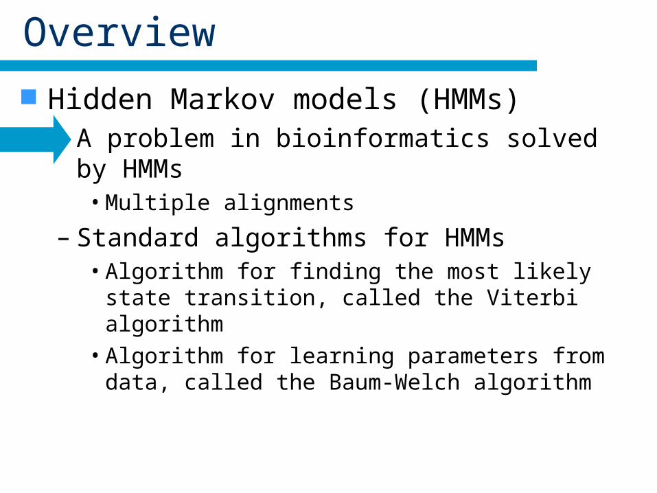
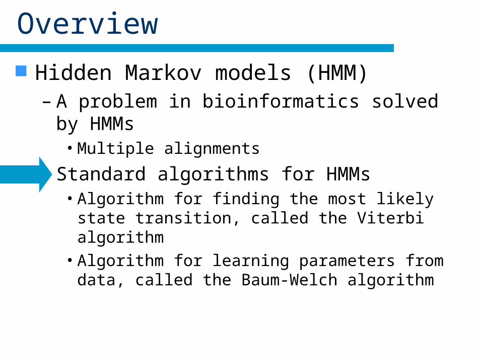
Overview
Hidden Markov models (HMMs)– A problem in bioinformatics solved by HMMs
• Multiple alignments
– Standard algorithms for HMMs• Algorithm for finding the most likely state transition, called
the Viterbi algorithm
• Algorithm for learning parameters from data, called the Baum-Welch algorithm
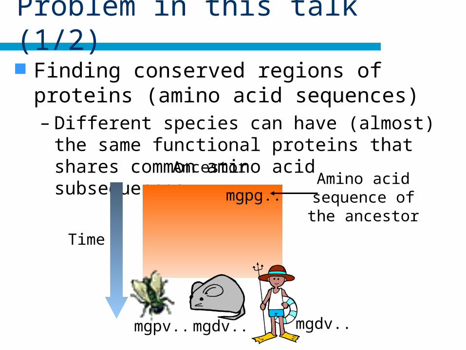
Problem in this talk (1/2)
Finding conserved regions of proteins (amino acid sequences)– Different species can have (almost) the same
functional proteins that shares common amino acid subsequences. Ancestor
mgdv.. mgdv..mgpv..
Time
Amino acidsequence ofthe ancestor
mgpg..
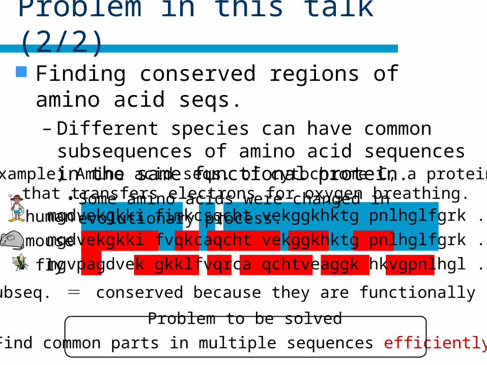
Problem in this talk (2/2)
Finding conserved regions of amino acid seqs.– Different species can have common subsequences of
amino acid sequences in the same functional protein.• Some amino acids were changed in evolutionary process.
Example) Amino acid seqs. of cytochrome C, a protein that transfers electrons for oxygen breathing.
Find common parts in multiple sequences efficiently.
Problem to be solved
Common subseq. = conserved because they are functionally important?
humanmgdvekgkki fimkcsqcht vekggkhktg pnlhglfgrk ...
mousemgdvekgkki fvqkcaqcht vekggkhktg pnlhglfgrk ...
flymgvpagdvek gkklfvqrca qchtveaggk hkvgpnlhgl ...
Comparison of sequences
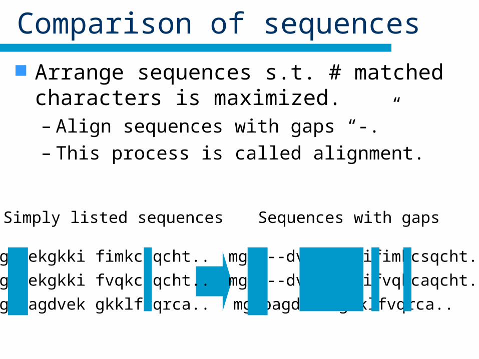
Arrange sequences s.t. # matched characters is maximized.– Align sequences with gaps “-.”– This process is called alignment.
Simply listed sequences
mgdvekgkki fimkcsqcht..
mgdvekgkki fvqkcaqcht..
mgvpagdvek gkklfvqrca..
Sequences with gaps
mg----dvek gkkifimkcsqcht..
mg----dvek gkkifvqkcaqcht..
mgvpagdvek gkklfvqrca..
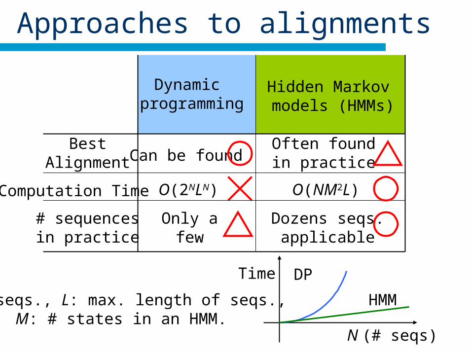
Approaches to alignments
N: # seqs., L: max. length of seqs., M: # states in an HMM.
Dynamic programming
Hidden Markov models (HMMs)
BestAlignment
# sequencesin practice
Computation Time
Can be foundOften foundin practice
N (# seqs)
Time DP
HMM
O(2NLN) O(NM2L)
Only afew
Dozens seqs.applicable
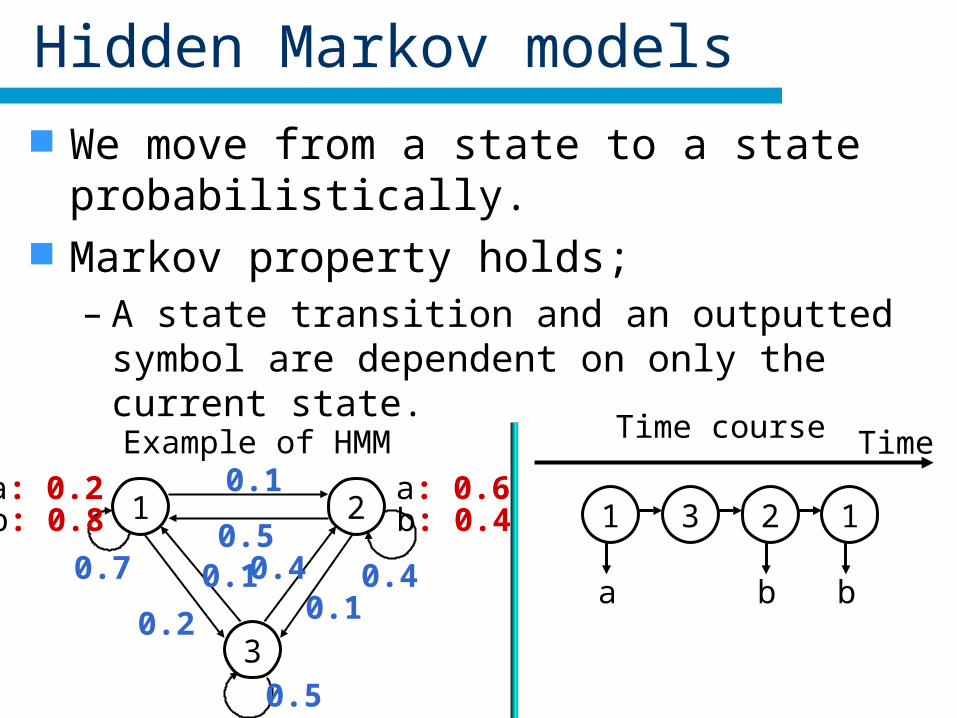
Hidden Markov models
We move from a state to a state probabilistically. Markov property holds;
– A state transition and an outputted symbol are dependent on only the current state.
Example of HMM
1 2
3
0.7
0.1
0.2
0.1 0.4
0.5
0.50.4
0.1
a: 0.2b: 0.8
a: 0.6b: 0.4
Time course Time
1
a
3 2
b
1
b
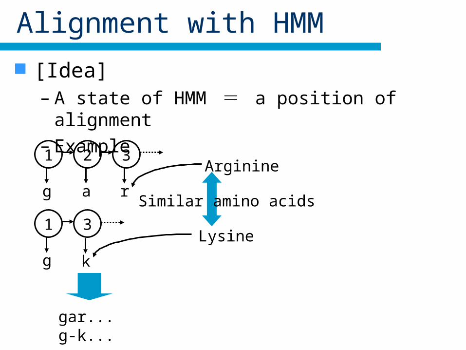
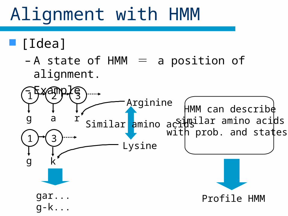
Alignment with HMM
[Idea]– A state of HMM = a position of alignment– Example
1
g
2 3
r
1
g
3
k
a
gar...g-k...
Arginine
Lysine
Similar amino acids
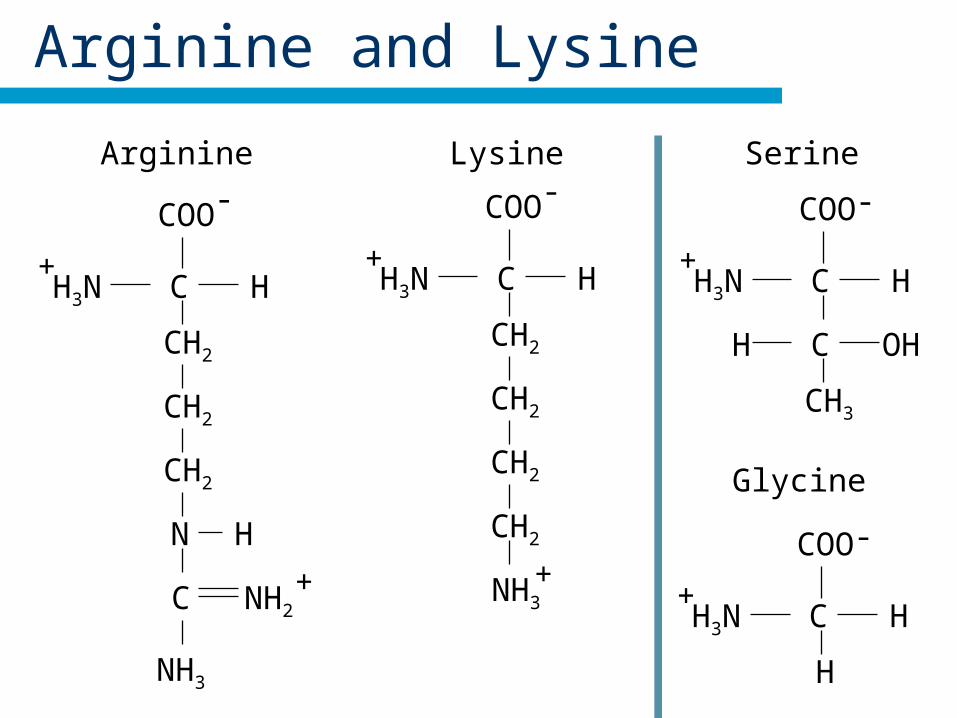
Arginine and Lysine
Arginine Lysine-COO
H3N+
C H
NH3
CH2
CH2
CH2
CH2
+
COO-
H3N+
C H
C
CH2
CH2
CH2
HN
NH3
NH2+
Serine
COO-
H3N+
C H
CH3
C OHH
-COO
H3N+
C H
H
Glycine
Alignment with HMM
[Idea]– A state of HMM = a position of alignment.– Example
1
g
2 3
r
1
g
3
k
a
gar...g-k...
Arginine
Lysine
Similar amino acids
Profile HMM
HMM can describesimilar amino acids
with prob. and states.
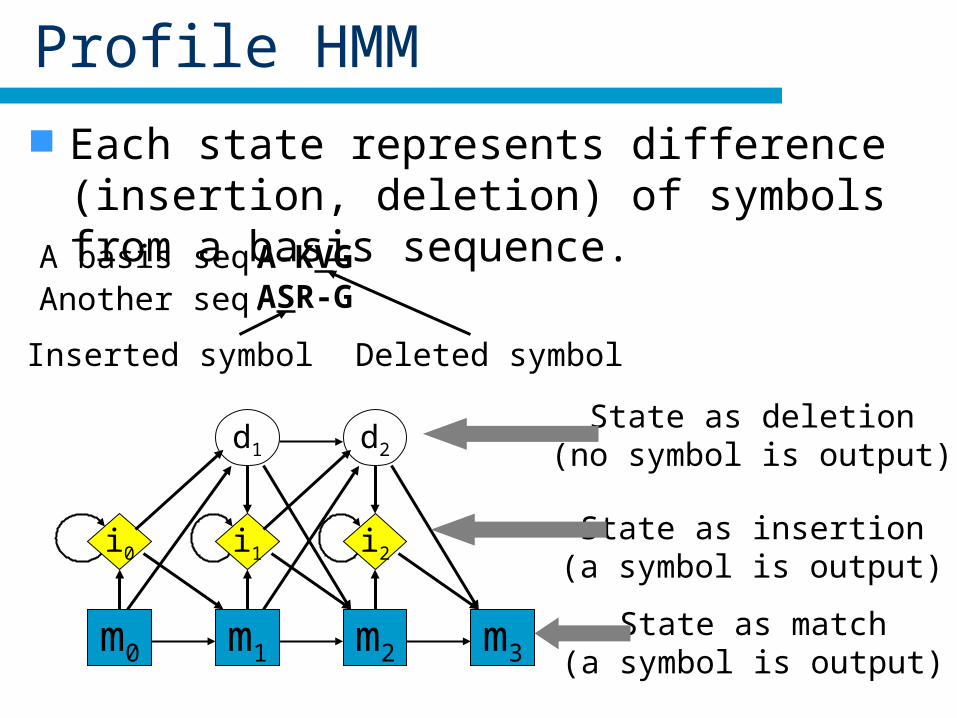
Profile HMM
Each state represents difference (insertion, deletion) of symbols from a basis sequence.
m0
i0
d1
m1
i1
d2
m2
i2
m3State as match
(a symbol is output)
State as insertion(a symbol is output)
State as deletion(no symbol is output)
A basis seq. A-KVG
Inserted symbol Deleted symbol
ASR-GAnother seq.
Matched symbols
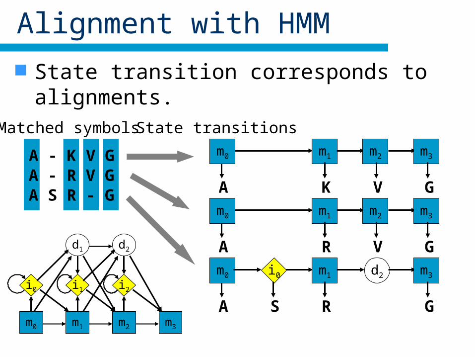
Alignment with HMM
State transition corresponds to alignments.
A - K V GA - R V GA S R - G
State transitions
m1 m2 m3m0
A K V Gm1 m2 m3m0
A R V Gm1 d2 m3m0
A R G
i0
Sm0
i0
d1
m1
i1
d2
m2
i2
m3
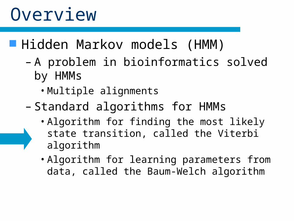
Overview
Hidden Markov models (HMM)– A problem in bioinformatics solved by HMMs
• Multiple alignments
– Standard algorithms for HMMs• Algorithm for finding the most likely state transition, called
the Viterbi algorithm
• Algorithm for learning parameters from data, called the Baum-Welch algorithm
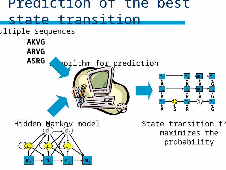
Prediction of the best state transition
Algorithm for prediction
Multiple sequences
AKVGARVGASRG
m0
i0
d1
m1
i1
d2
m2
i2
m3
Hidden Markov model State transition thatmaximizes the
probability
m1 m2 m3m0
A K V Gm1 m2 m3m0
A R V Gm1 d2 m3m0
A R G
i0
S
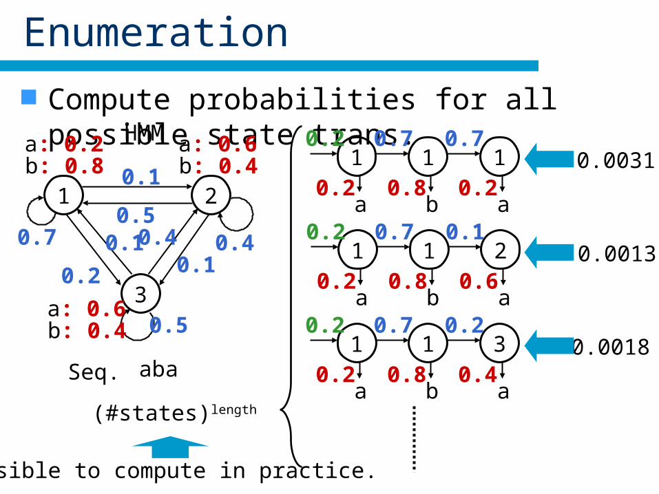
Enumeration
Compute probabilities for all possible state trans.
Seq. aba
10.2
a0.2
10.7
b0.8
10.7
a0.2
10.2
a0.2
10.7
b0.8
20.1
a0.6
10.2
a0.2
10.7
b0.8
30.2
a0.4
0.0031
0.0013
0.0018
HMM
1 2
3
0.7
0.1
0.2
0.1 0.4
0.5
0.50.4
0.1
a: 0.2b: 0.8
a: 0.6b: 0.4
a: 0.6b: 0.4
(#states)length
Impossible to compute in practice.
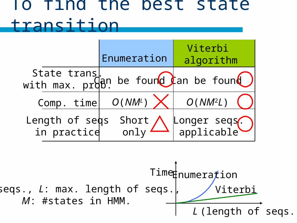
To find the best state transition
N: # seqs., L: max. length of seqs., M: #states in HMM.
EnumerationViterbi
algorithmState trans.
with max. prob.
Length of seqsin practice
Comp. time
Can be found
O(NML) O(NM2L)
Shortonly
Longer seqs.applicable
Can be found
L (length of seqs.)
Time Enumeration
Viterbi
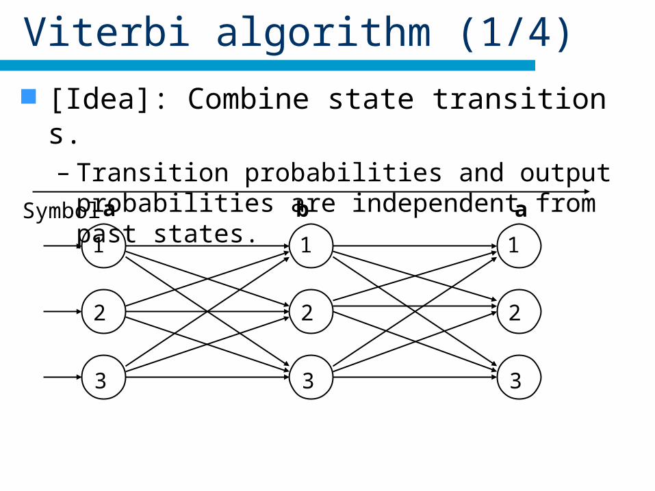
Viterbi algorithm (1/4)
[Idea]: Combine state transitions.– Transition probabilities and output probabilities are
independent from past states.
Symbol a b a
1
2
3
1
2
3
1
2
3
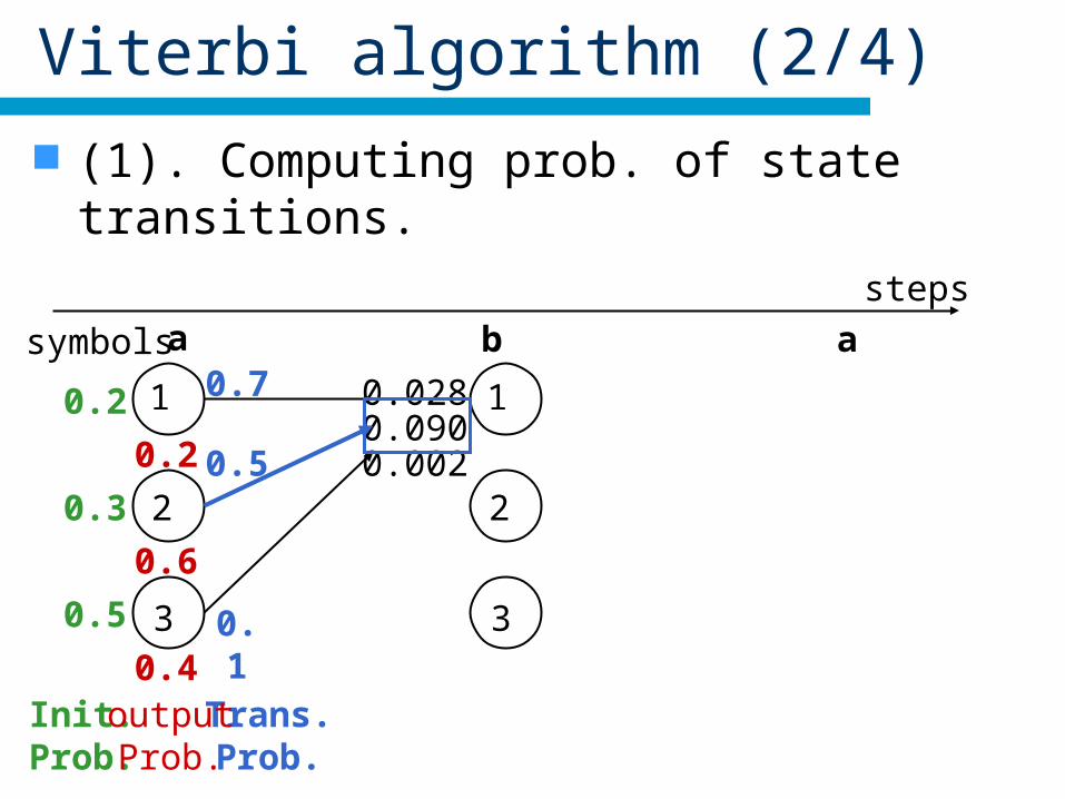
Viterbi algorithm (2/4)
(1). Computing prob. of state transitions.
Init.Prob.
0.2 1
0.3 2
0.5 3
steps
Trans.Prob.
1
2
3
symbols a b a
0.2
0.6
0.4outputProb.
0.7 0.028
0.50.090
0.1
0.002
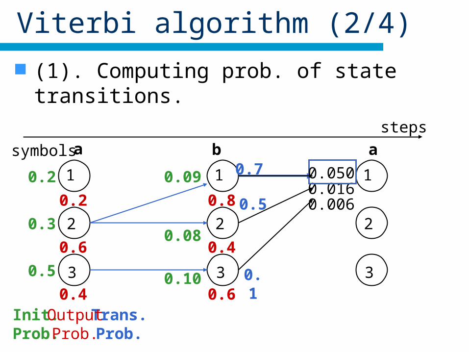
Viterbi algorithm (2/4)
(1). Computing prob. of state transitions.
Init.Prob.
0.2
0.3
0.5
1
2
3
steps
Trans.Prob.
1
2
3
symbols a b a
0.2
0.6
0.4OutputProb.
0.08
0.09
0.10
1
2
3
0.8
0.4
0.6
0.50.016
0.1
0.006
0.0500.7
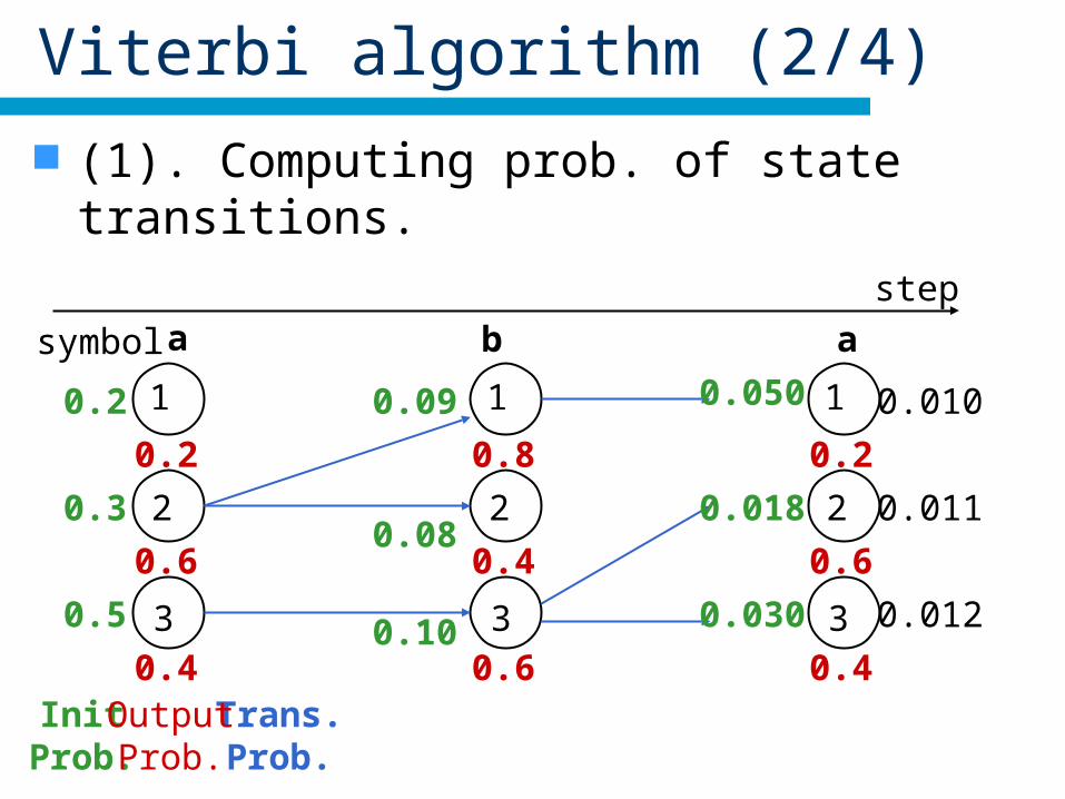
Viterbi algorithm (2/4)
(1). Computing prob. of state transitions.
InitProb.
0.2
0.3
0.5
1
2
3
step
Trans.Prob.
1
2
3
symbol a b a
0.2
0.6
0.4OutputProb.
0.08
0.09
0.10
1
2
3
0.8
0.4
0.6
0.050
0.018
0.030
0.2
0.6
0.4
0.010
0.011
0.012
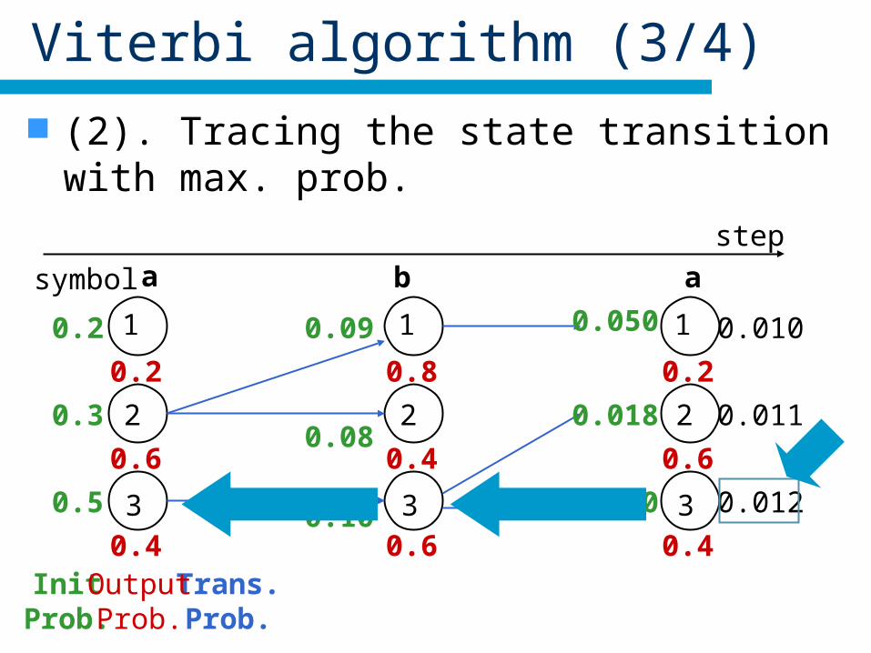
Viterbi algorithm (3/4)
(2). Tracing the state transition with max. prob.
InitProb.
0.2
0.3
0.5
1
2
3
step
Trans.Prob.
1
2
3
symbol a b a
0.2
0.6
0.4OutputProb.
0.08
0.09
0.10
1
2
3
0.8
0.4
0.6
0.050
0.018
0.030
0.2
0.6
0.4
0.010
0.011
0.012
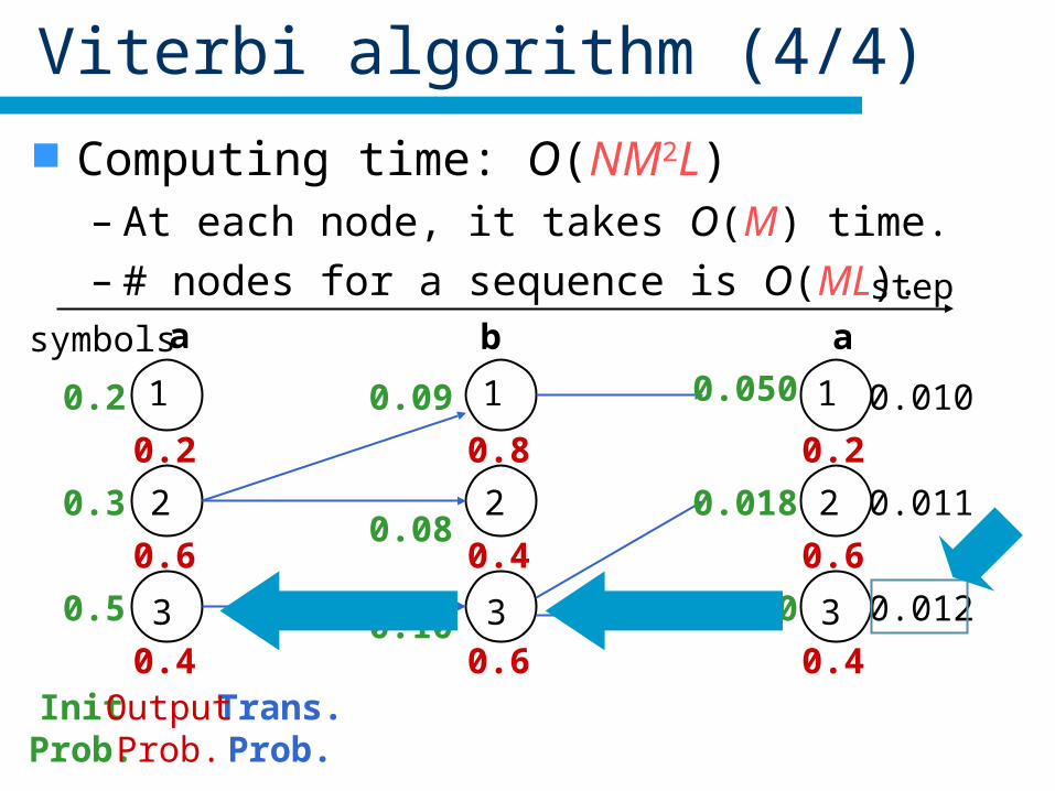
Viterbi algorithm (4/4)
Computing time: O(NM2L)– At each node, it takes O(M) time.– # nodes for a sequence is O(ML). step
InitProb.
0.2
0.3
0.5
1
2
3
Trans. Prob.
1
2
3
symbols a b a
0.2
0.6
0.4OutputProb.
0.08
0.09
0.10
1
2
3
0.8
0.4
0.6
0.050
0.018
0.030
0.2
0.6
0.4
0.010
0.011
0.012
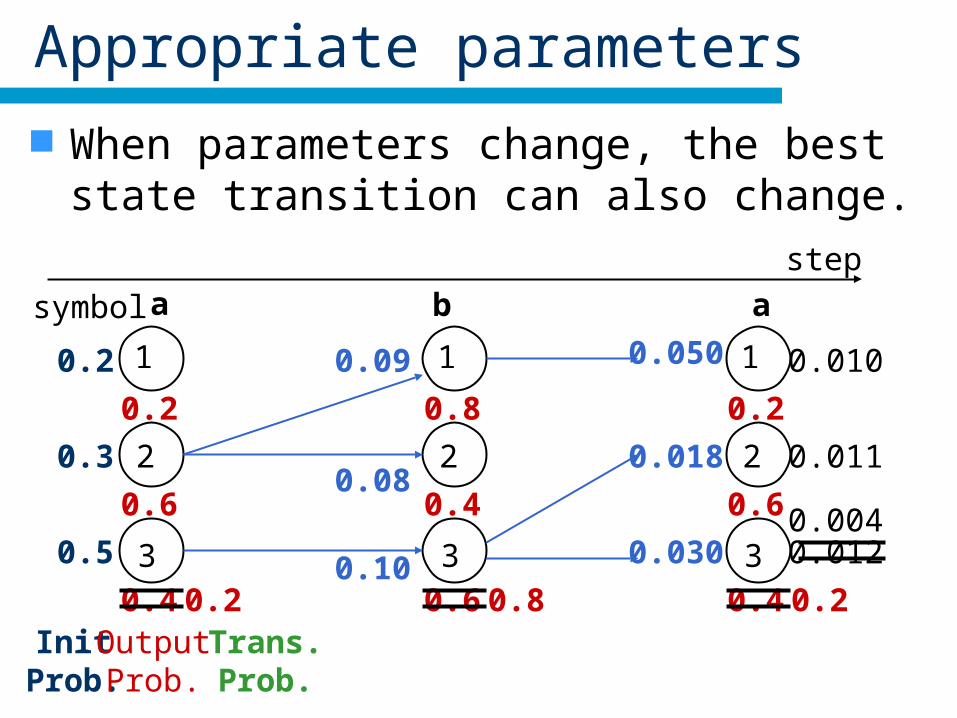
Appropriate parameters
When parameters change, the best state transition can also change.
InitProb.
0.2
0.3
0.5
1
2
3
step
Trans.Prob.
1
2
3
symbol a b a
0.2
0.6
0.4OutputProb.
0.08
0.09
0.10
1
2
3
0.8
0.4
0.6
0.050
0.018
0.030
0.2
0.6
0.4
0.010
0.011
0.012
0.2 0.8 0.2
0.004
Overview
Hidden Markov models (HMM)– A problem in bioinformatics solved by HMMs
• Multiple alignments
– Standard algorithms for HMMs• Algorithm for finding the most likely state transition, called
the Viterbi algorithm
• Algorithm for learning parameters from data, called the Baum-Welch algorithm
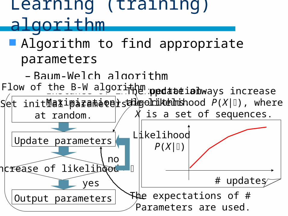
Learning (training) algorithm
Algorithm to find appropriate parameters– Baum-Welch algorithm
• Instance of EM (Expectation-Maximization) algorithms.
Set initial parametersat random.
# updates
Likelihood P(X|)Update parameters
Increase of likelihood<
Output parameters
yes
no
Flow of the B-W algorithm The update always increase the likelihood P(X|), where
X is a set of sequences.
The expectations of # Parameters are used.
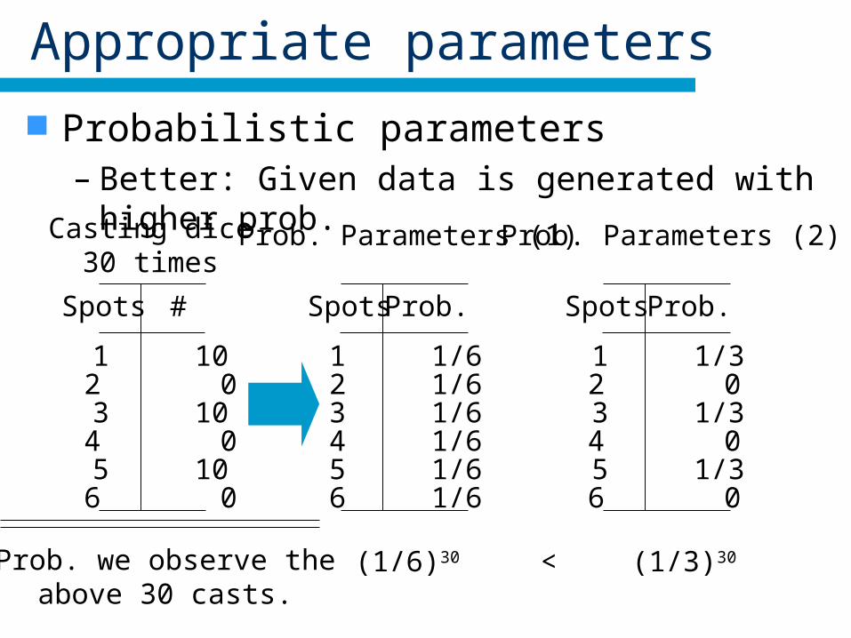
Appropriate parameters
Probabilistic parameters– Better: Given data is generated with higher prob.
Casting dice30 times
Prob. Parameters (1) Prob. Parameters (2)
Prob. we observe theabove 30 casts.
(1/6)30 (1/3)30<
Spots
1 102 03 104 05 106 0
# Spots
1 1/62 1/63 1/64 1/65 1/66 1/6
Prob. Spots
1 1/32 03 1/34 05 1/36 0
Prob.
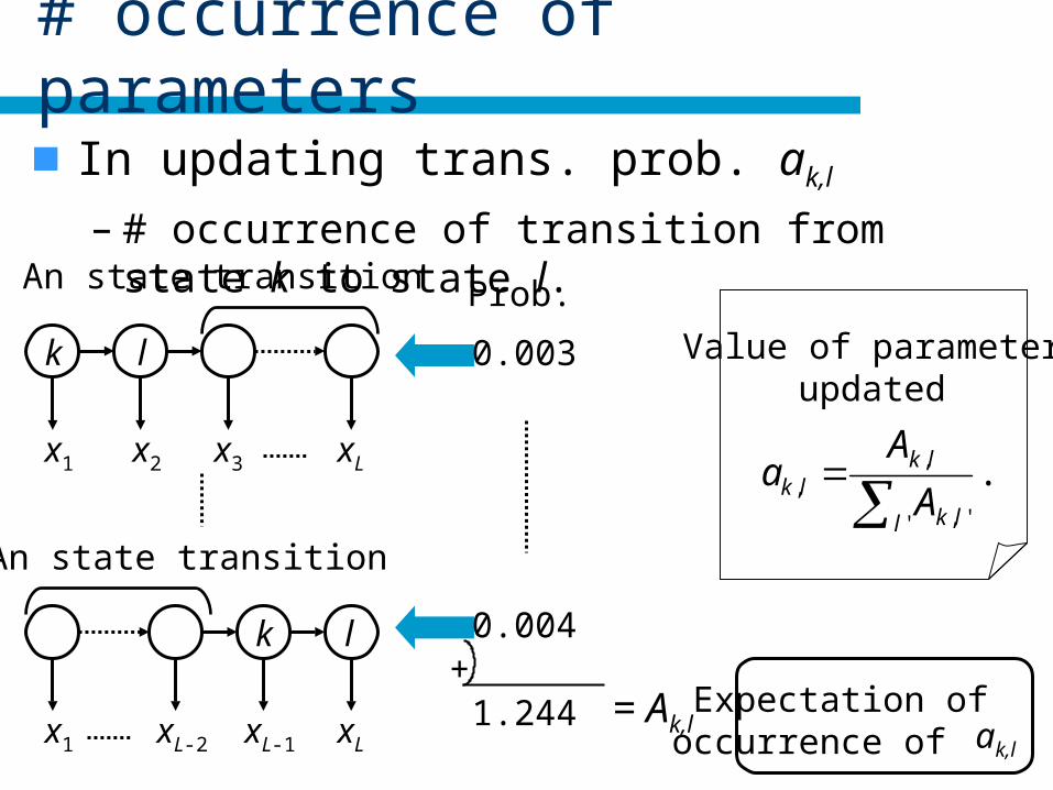
# occurrence of parameters
In updating trans. prob. ak,l
– # occurrence of transition from state k to state l.
An state transition
x1 xL-1
k l
xLxL-2
An state transition
x1 x2
k l
xLx3
Prob.
+1.244 = Ak,l ak,l
Expectation of occurrence of
Value of parameterupdated
.' ',
,,
l lk
lklk A
Aa
0.003
0.004
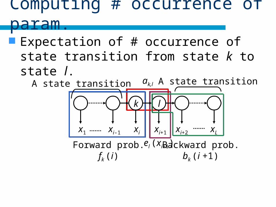
el (xi+1)
xi+1
ak,l
Forward prob.fk (i)
Computing # occurrence of param.
Expectation of # occurrence of state transition from state k to state l.
l
xi-1 xix1
k
A state transition
xi+2
A state transition
xL
Backward prob.bk (i +1)
a1,k
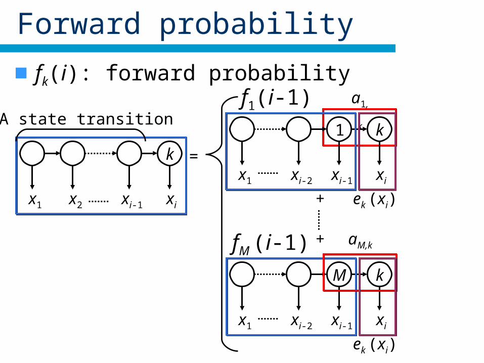
Forward probability
fk(i): forward probability
A state transition
x1 x2 xi-1
k
xi
=
+
+
x1 xi-2 xi-1
k
xi
1
x1 xi-2 xi-1
k
xi
M
f1(i-1)
ek (xi)
fM (i-1) aM,k
ek (xi)
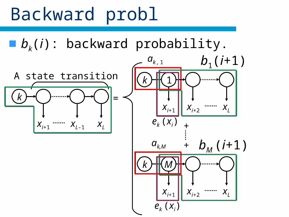
Backward probl
bk(i): backward probability.
=
+
+
xi+2xi+1
k
xL
M
bM (i+1)
A state transition
xL-1xi+1
k
xL
ak , 1
xi+2
k
xL
1
xi+1
b1(i+1)
ek (xi)
ak,M
ek (xi)
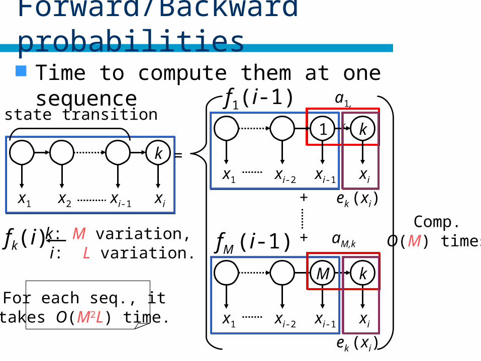
Forward/Backward probabilities
Time to compute them at one sequence
aM,k
ek (xi)
a1,k
A state transition
x1 x2 xi-1
k
xi
=x1 xi-2 xi-1
k
xi
+
+
x1 xi-2 xi-1
k
xi
1
M
f1(i-1)
fM (i-1)
ek (xi)
fk(i) k: M variation, i: L variation.
Comp.O(M) times
For each seq., it takes O(M2L) time.
Conclusion
Alignment of multiple sequences– To find conserved regions of protein sequences.
Hidden Markov models (HMM)– profile HMM
• Describes alignments of multiple sequences.
– Prediction algorithm• Viterbi algorithm
– Learning (training) algorithm• Baum-Welch algorithm
– For efficiency, the forward and backward probabilities are used.