Hidden Markov Models in Practice

Based on materials from Jacky Birrell,

Tomáš Kolský

Outline

• Markov Chains

• Extension to HMM

• Urn and Ball

• Modelling BLAST Similarity Matches

• Information Sources

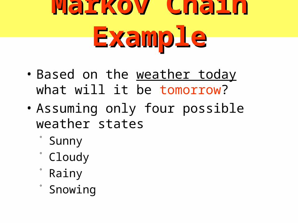
Markov Chain ExampleMarkov Chain Example

• Based on the weather today what will it be tomorrow?

• Assuming only four possible weather states Sunny Cloudy Rainy Snowing

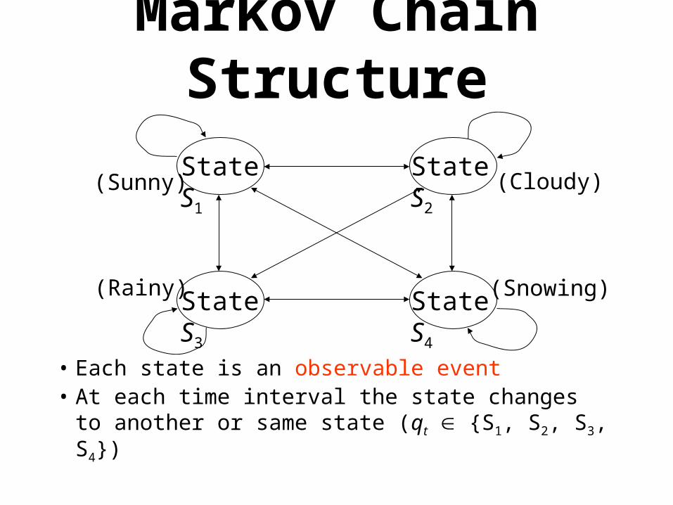
Markov Chain Structure

• Each state is an observable event• At each time interval the state changes to

another or same state (qt {S1, S2, S3, S4})

State S1 State S2

State S3 State S4

(Sunny)

(Snowing)(Rainy)

(Cloudy)

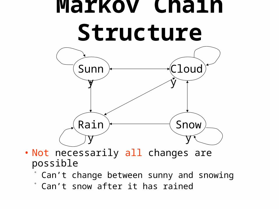
Markov Chain Structure

• Not necessarily all changes are possible Can’t change between sunny and snowing Can’t snow after it has rained

Sunny Cloudy

Rainy Snowy

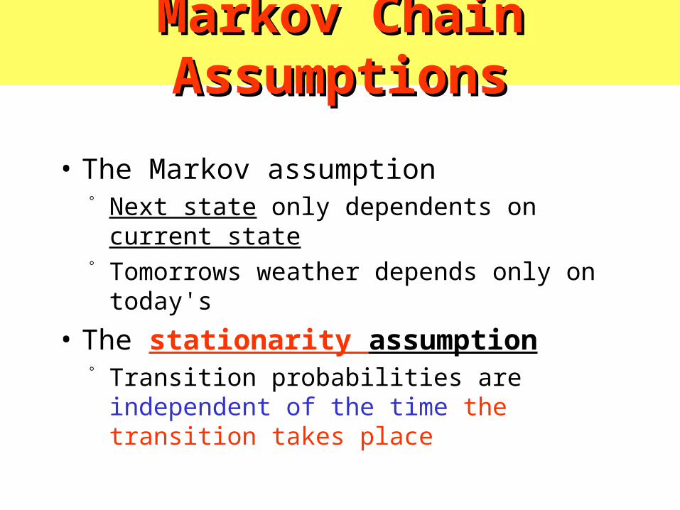
Markov Chain AssumptionsMarkov Chain Assumptions

• The Markov assumption Next state only dependents on current state Tomorrows weather depends only on today's

• The stationarity assumption Transition probabilities are independent of the

time the transition takes place

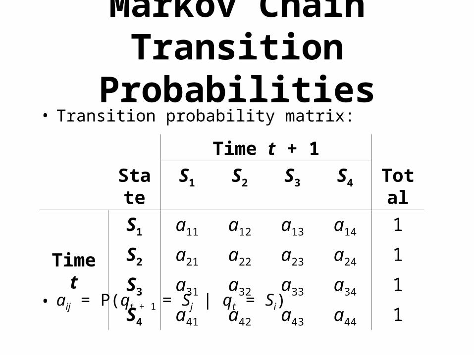
Markov Chain Transition Probabilities

• Transition probability matrix:

• aij = P(qt + 1 = Sj | qt = Si)

Time t + 1

State S1 S2 S3 S4 Total

Time t

S1 a11 a12 a13 a14 1

S2 a21 a22 a23 a24 1

S3 a31 a32 a33 a34 1

S4 a41 a42 a43 a44 1

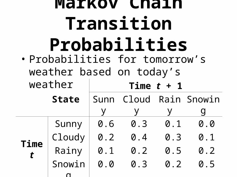
Markov Chain Transition Probabilities

• Probabilities for tomorrow’s weather based on today’s weather

Time t + 1

State Sunny Cloudy Rainy Snowing

Time t

Sunny 0.6 0.3 0.1 0.0

Cloudy 0.2 0.4 0.3 0.1

Rainy 0.1 0.2 0.5 0.2

Snowing 0.0 0.3 0.2 0.5

Extension to HMM

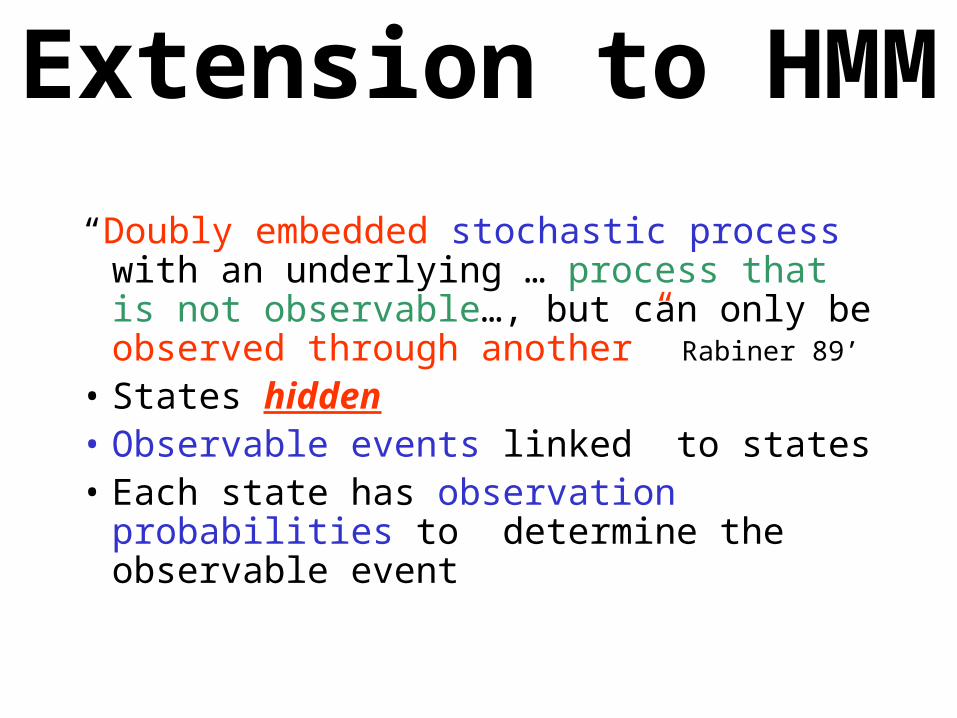
“Doubly embedded stochastic process with an underlying … process that is not observable…, but can only be observed through another” Rabiner 89’

• States hidden• Observable events linked to states• Each state has observation probabilities to

determine the observable event

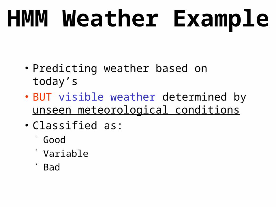
HMM Weather Example

• Predicting weather based on today’s

• BUT visible weather determined by unseen meteorological conditions

• Classified as: Good Variable Bad

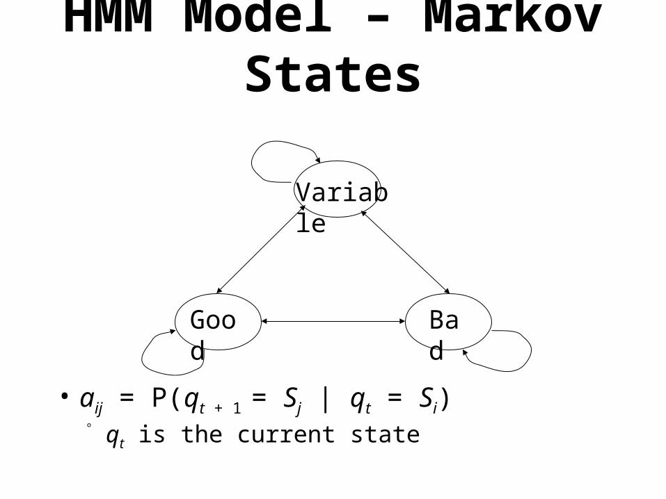
HMM Model – Markov States

• aij = P(qt + 1 = Sj | qt = Si) qt is the current state

Good

Variable

Bad

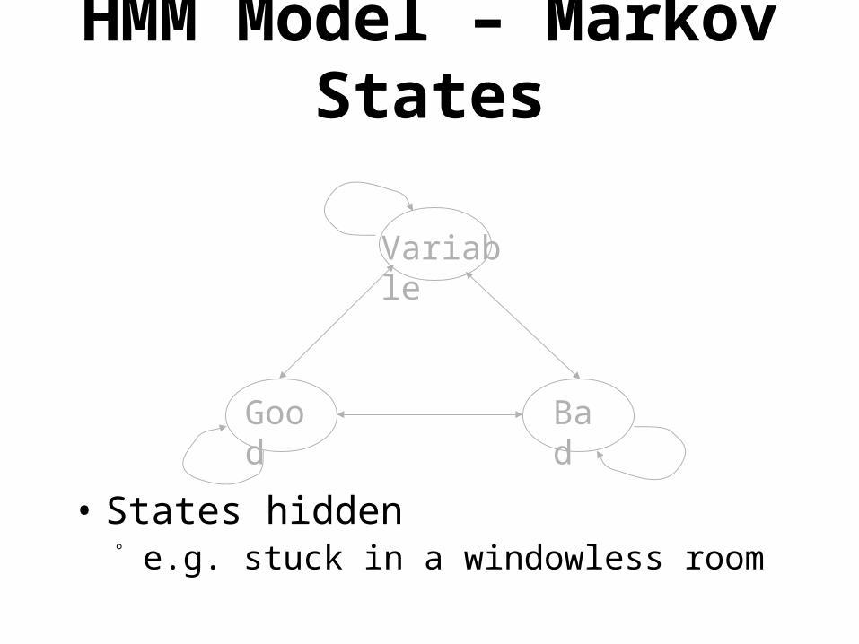
HMM Model – Markov States

• States hidden e.g. stuck in a windowless room

Good Bad

Variable

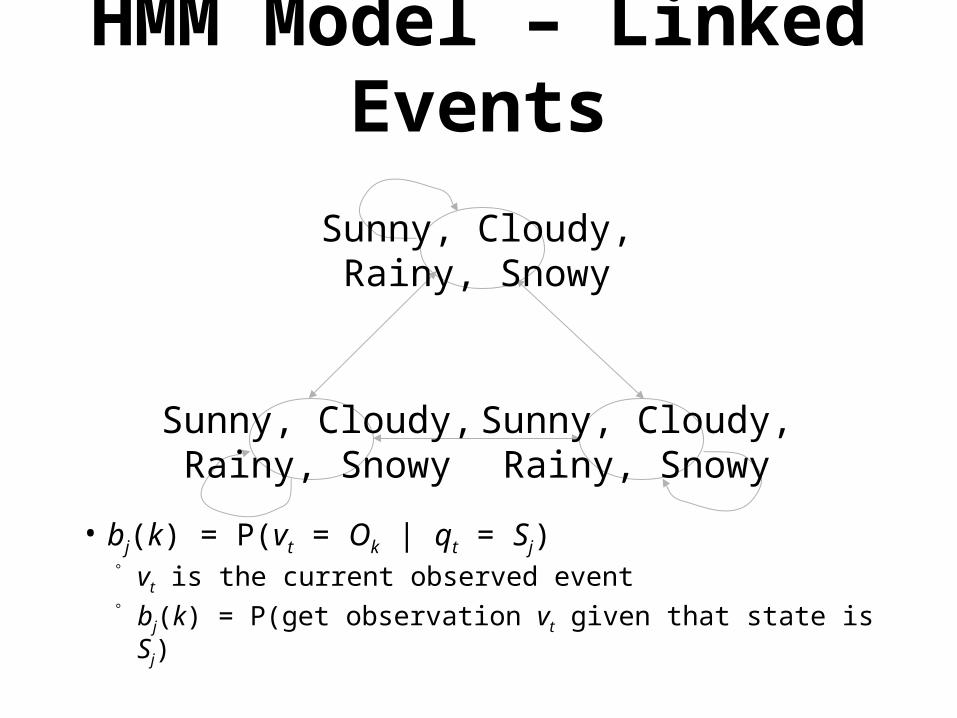
HMM Model – Linked Events

• bj(k) = P(vt = Ok | qt = Sj) vt is the current observed event bj(k) = P(get observation vt given that state is Sj)

Sunny, Cloudy,Rainy, Snowy

Sunny, Cloudy,Rainy, Snowy

Sunny, Cloudy,Rainy, Snowy

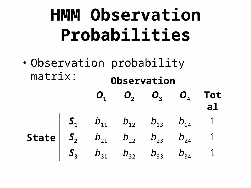
HMM Observation Probabilities

• Observation probability matrix:

Observation

O1 O2 O3 O4 Total

State

S1 b11 b12 b13 b14 1

S2 b21 b22 b23 b24 1

S3 b31 b32 b33 b34 1

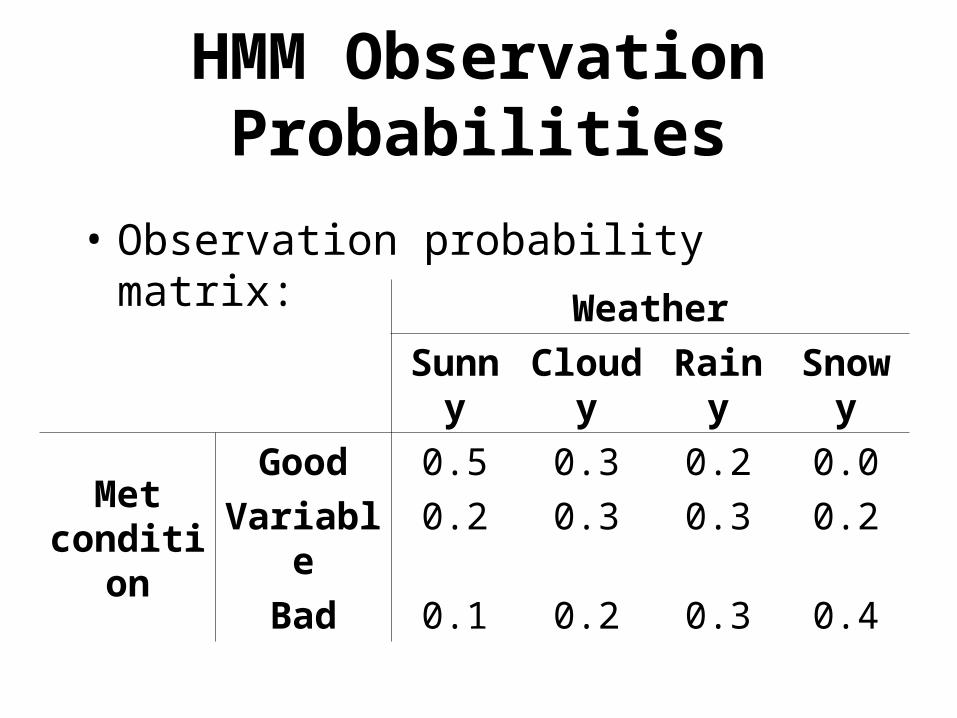
HMM Observation Probabilities

• Observation probability matrix:

Weather

Sunny Cloudy Rainy Snowy

Met condition

Good 0.5 0.3 0.2 0.0

Variable 0.2 0.3 0.3 0.2

Bad 0.1 0.2 0.3 0.4

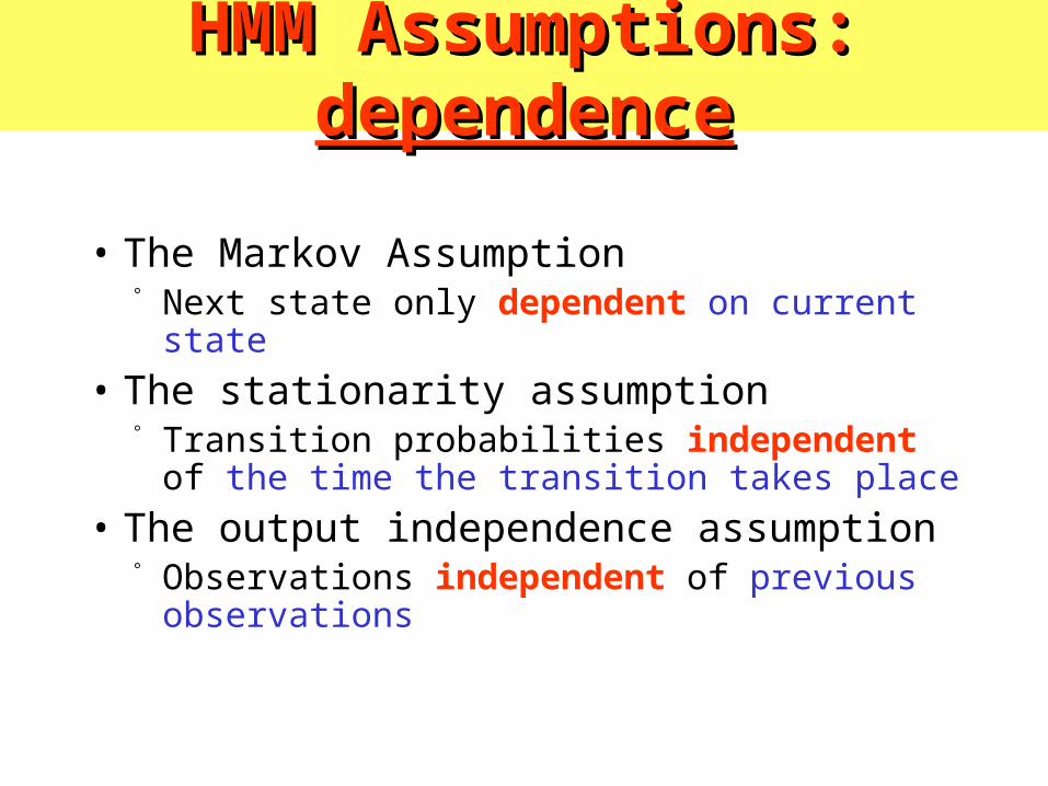
HMM Assumptions: HMM Assumptions: dependencedependence

• The Markov Assumption Next state only dependent on current state

• The stationarity assumption Transition probabilities independent of the

time the transition takes place

• The output independence assumption Observations independent of previous

observations

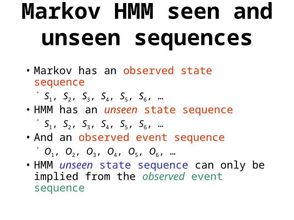
Markov HMM seen and unseen sequences

• Markov has an observed state sequence S1, S2, S3, S4, S5, S6, …

• HMM has an unseen state sequence S1, S2, S3, S4, S5, S6, …

• And an observed event sequence O1, O2, O3, O4, O5, O6, …

• HMM unseen state sequence can only be implied from the observed event sequence

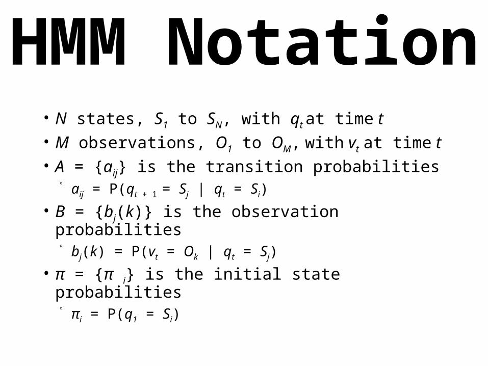
HMM Notation• N states, S1 to SN, with qt at time t• M observations, O1 to OM, with vt at time t• A = {aij} is the transition probabilities

aij = P(qt + 1 = Sj | qt = Si)

• B = {bj(k)} is the observation probabilities bj(k) = P(vt = Ok | qt = Sj)

• π = {π i} is the initial state probabilities πi = P(q1 = Si)

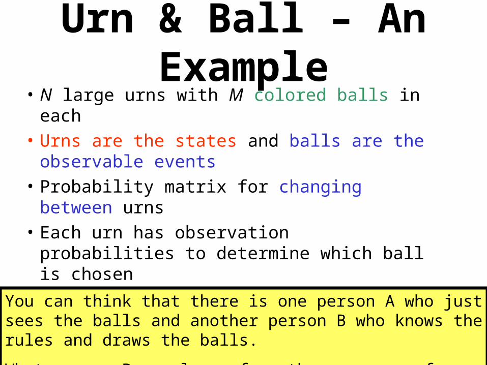
Urn & Ball – An Example• N large urns with M colored balls in each

• Urns are the states and balls are the observable events

• Probability matrix for changing between urns

• Each urn has observation probabilities to determine which ball is chosen

You can think that there is one person A who just sees the balls and another person B who knows the rules and draws the balls.

What person B can learn from the sequence of balls seen?

Urn & Ball – An Example

P(red) = b1(1) P(red) = b2(1) P(red) = b3(1)

P(blue) = b1(2) P(blue) = b2(2) P(blue) = b3(2)

P(green) = b1(3) P(green) = b2(3) P(green) = b3(3)

P(purple) = b1(4) P(purple) = b2(4) P(purple) = b3(4)… … …

Urn 1 Urn 2 Urn 3

• N large urns with M colored balls in each

• Urns are the states and balls are the observable events

• Probability matrix for changing between urns

• Each urn has observation probabilities to determine which ball is chosen

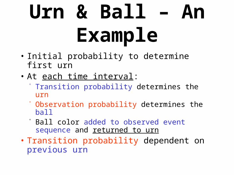
Urn & Ball – An Example

• Initial probability to determine first urn• At each time interval:

Transition probability determines the urn Observation probability determines the ball Ball color added to observed event sequence

and returned to urn

• Transition probability dependent on previous urn

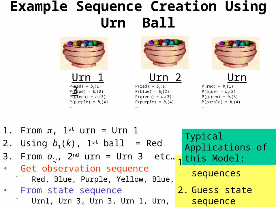
Example Sequence Creation Using Urn Ball

1. From , 1st urn = Urn 1

2. Using b1(k), 1st ball = Red

3. From a1j, 2nd urn = Urn 3 etc…• Get observation sequence

Red, Blue, Purple, Yellow, Blue, Blue

• From state sequence Urn1, Urn 3, Urn 3, Urn 1, Urn, 2, Urn 1

P(red) = b1(1) P(red) = b2(1) P(red) = b3(1) P(blue) = b1(2) P(blue) = b2(2) P(blue) = b3(2)P(green) = b1(3) P(green) = b2(3) P(green) = b3(3)P(purple) = b1(4) P(purple) = b2(4) P(purple) = b3(4)… … …

Urn 1 Urn 2 Urn 3

1. Generate sequences

2. Guess state sequence (state) by observing balls sequence

Typical Applications of this Model:

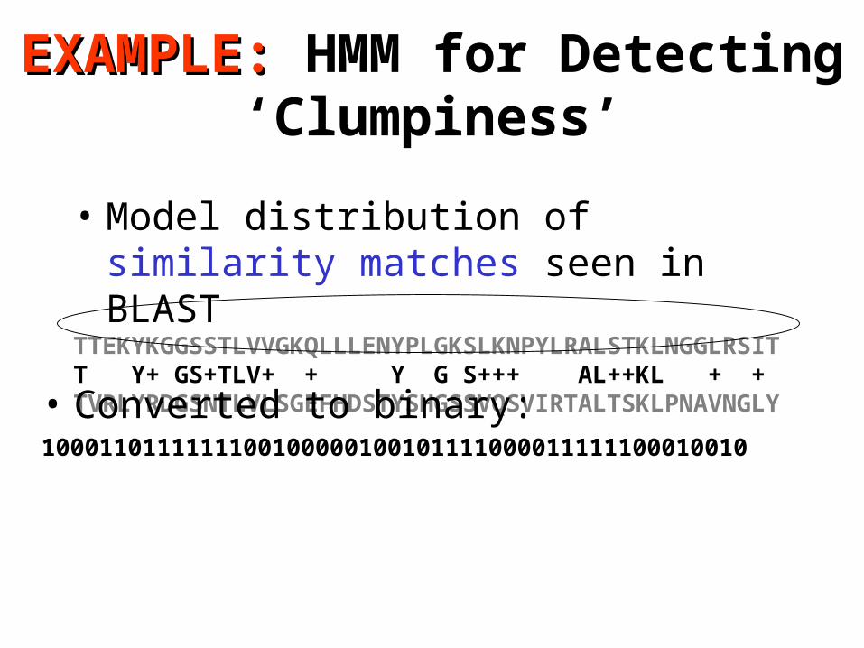
EXAMPLE:EXAMPLE: HMM for Detecting ‘Clumpiness’

• Model distribution of similarity matches seen in BLAST

TTEKYKGGSSTLVVGKQLLLENYPLGKSLKNPYLRALSTKLNGGLRSITT Y+ GS+TLV+ + Y G S+++ AL++KL + + TVRLYRDGSNTLVLSGEFHDSTYSHGSSVQSVIRTALTSKLPNAVNGLY

• Converted to binary:1000110111111100100000100101111000011111100010010

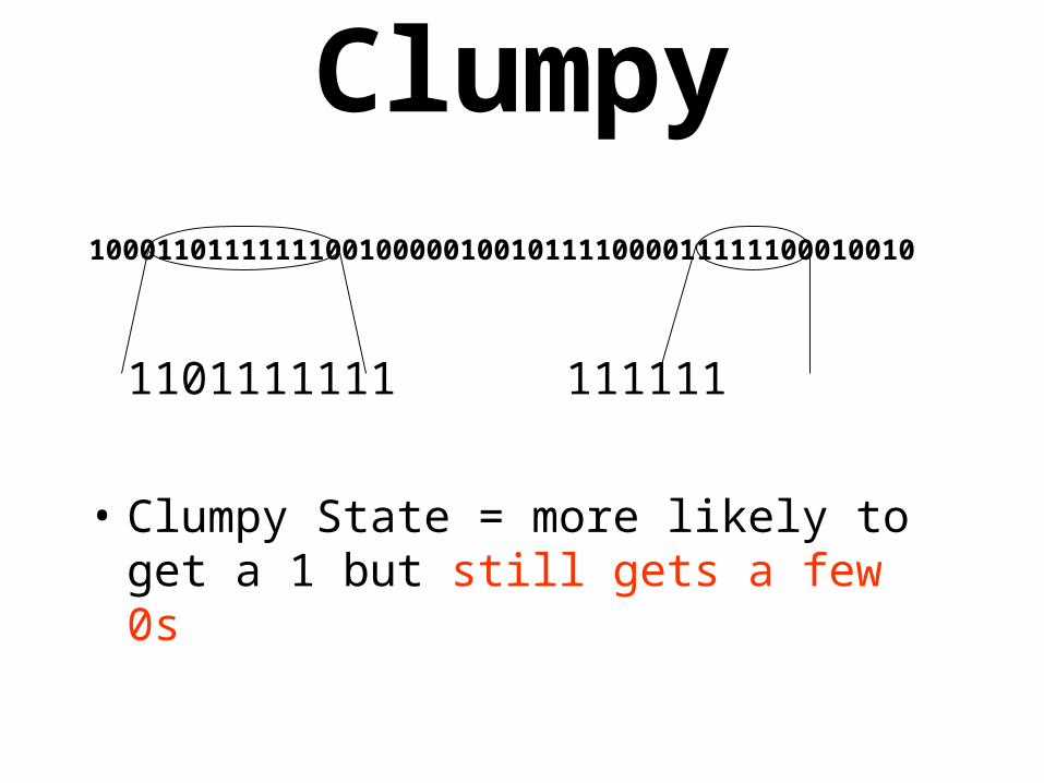
Clumpy1000110111111100100000100101111000011111100010010

1101111111 111111

• Clumpy State = more likely to get a 1 but still gets a few 0s

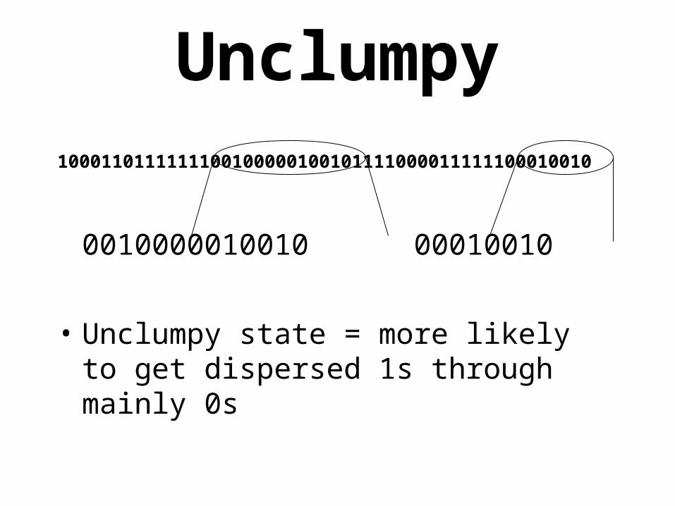
Unclumpy1000110111111100100000100101111000011111100010010

0010000010010 00010010

• Unclumpy state = more likely to get dispersed 1s through mainly 0s

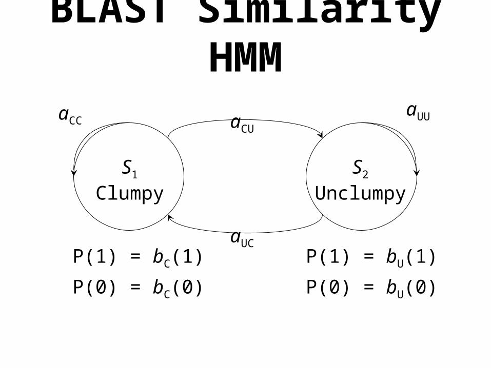
S1

ClumpyS2

Unclumpy

aCC aCU

aUU

aUC

BLAST Similarity HMM

P(1) = bC(1) P(1) = bU(1)

P(0) = bC(0) P(0) = bU(0)

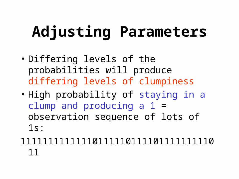
Adjusting Parameters

• Differing levels of the probabilities will produce differing levels of clumpiness

• High probability of staying in a clump and producing a 1 = observation sequence of lots of 1s:

1111111111111011111011110111111111011

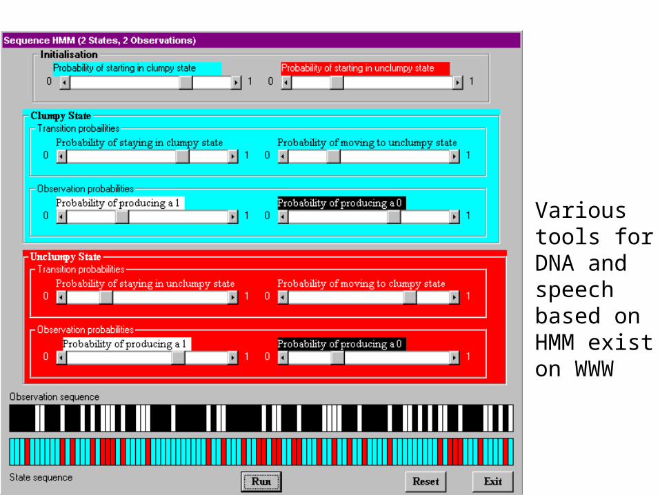
Various tools for DNA and speech based on HMM exist on WWW

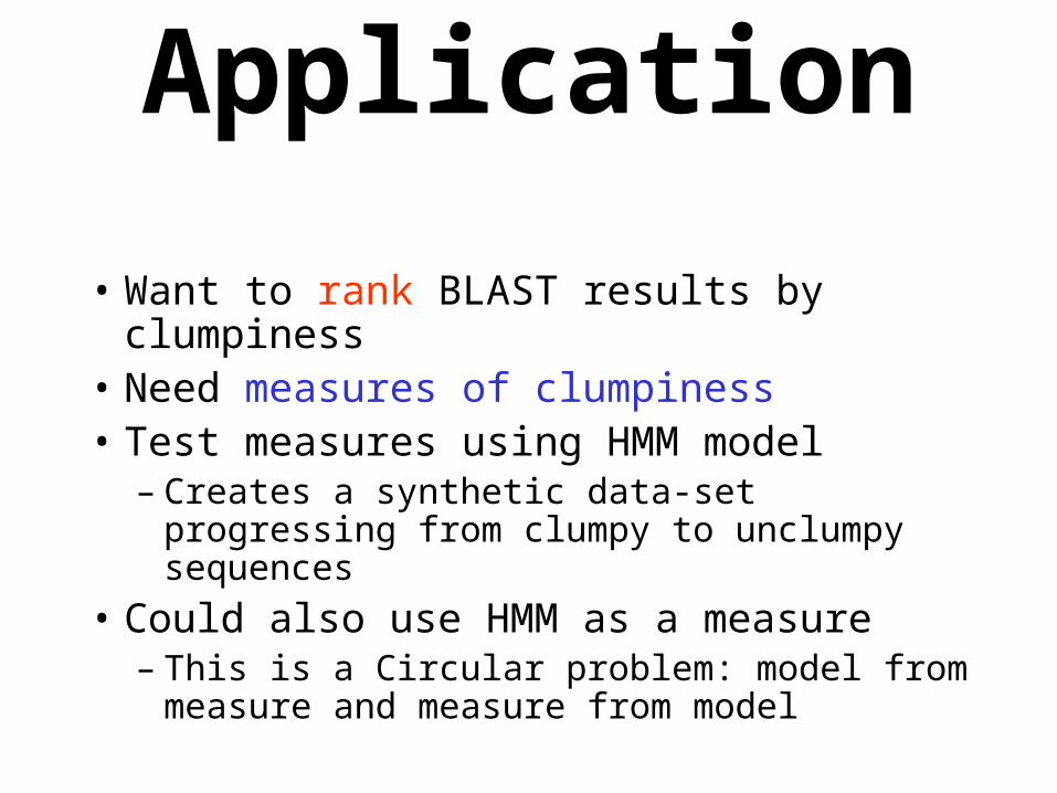
Application

• Want to rank BLAST results by clumpiness• Need measures of clumpiness• Test measures using HMM model

– Creates a synthetic data-set progressing from clumpy to unclumpy sequences

• Could also use HMM as a measure– This is a Circular problem: model from

measure and measure from model

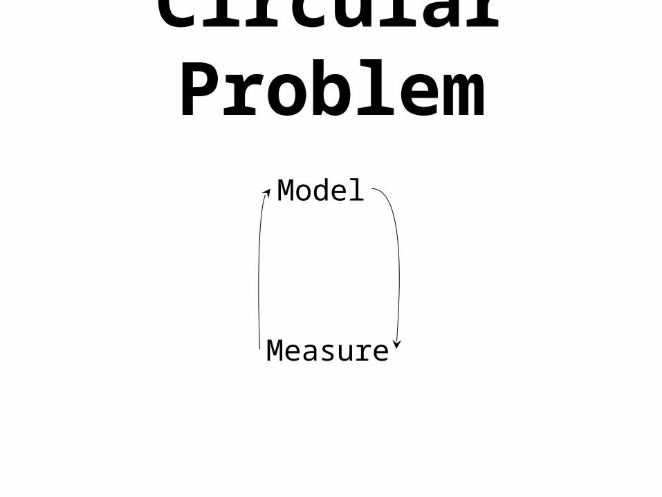
Circular Problem

Model

Measure

Applications in speech Applications in speech recognitionrecognition

• Hidden Markov Model of speech• State transitions and alignment probabilities• Searching all possible alignments• Dynamic Programming• Viterbi Alignment• Isolated Word Recognition

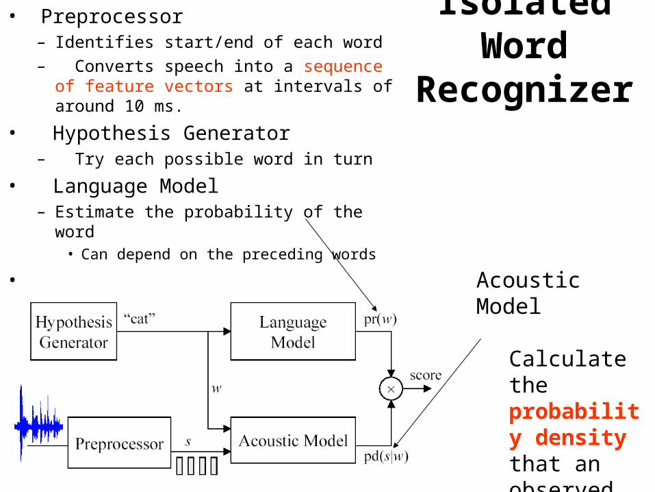
Isolated Word Recognizer

• Preprocessor– Identifies start/end of each word

– Converts speech into a sequence of feature vectors at intervals of around 10 ms.

• Hypothesis Generator– Try each possible word in turn

• Language Model– Estimate the probability of the word

• Can depend on the preceding words

• Acoustic Model

Calculate the probability density that an observed sequence of feature vectors corresponds to the chosen word

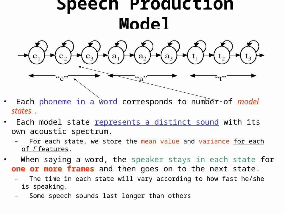
Speech Production Model

• Each phoneme in a word corresponds to number of model states .

• Each model state represents a distinct sound with its own acoustic spectrum.– For each state, we store the mean value and variance for each of F features.

• When saying a word, the speaker stays in each state for one or more frames and then goes on to the next state.– The time in each state will vary according to how fast he/she is speaking.

– Some speech sounds last longer than others

State Transitions

Average duration of 1/p frames

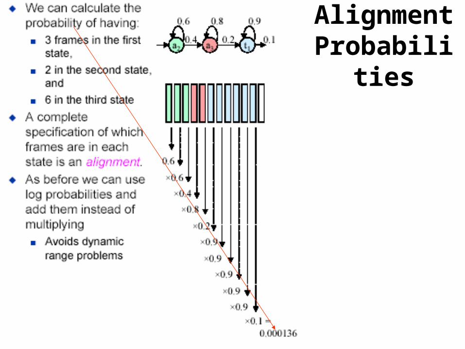
Alignment Probabilities

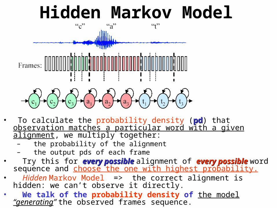
Hidden Markov Model

• To calculate the probability density (pdpd) that observation matches a particular word with a given alignment, we multiply together:– the probability of the alignment– the output pds of each frame

• Try this for every possibleevery possible alignment of every possibleevery possible word sequence and choose the one with highest probability.

• Hidden Markov Model => the correct alignment is hidden: we can’t observe it directly.

• We talk of the probability density of the model “generating” the observed frames sequence.

Hidden Markov Model Parameters

• A Hidden Markov Model for a word must specify the following parameters for state s:– The mean and variance for each of the F elements of the parameter vector: µs

and s 2.• These allow us to calculate ds(x): the output probability density of input frame x in

state s.– The transition probabilities as,j to every possible successor state.

• as,j is often zero for all j except j=s and j=s+1 it is then called a left-to-right, no skips model.

• For a Hidden Markov Model with S states we therefore have around (2F+1)S parameters.– A typical word might have S=15 and F=39 giving 1200 parameters in all.

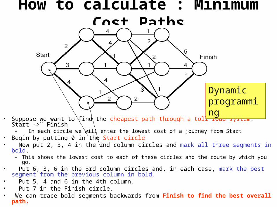
How to calculate : Minimum Cost Paths

• Suppose we want to find the cheapest path through a toll road system: Start ->¨ Finish– In each circle we will enter the lowest cost of a journey from Start

• Begin by putting 0 in the Start circle• Now put 2, 3, 4 in the 2nd column circles and mark all three segments in bold.

– This shows the lowest cost to each of these circles and the route by which you go.• Put 6, 3, 6 in the 3rd column circles and, in each case, mark the best segment from the

previous column in bold.• Put 5, 4 and 6 in the 4th column.• Put 7 in the Finish circle.• We can trace bold segments backwards from Finish to find the best overall path.

Dynamic programming

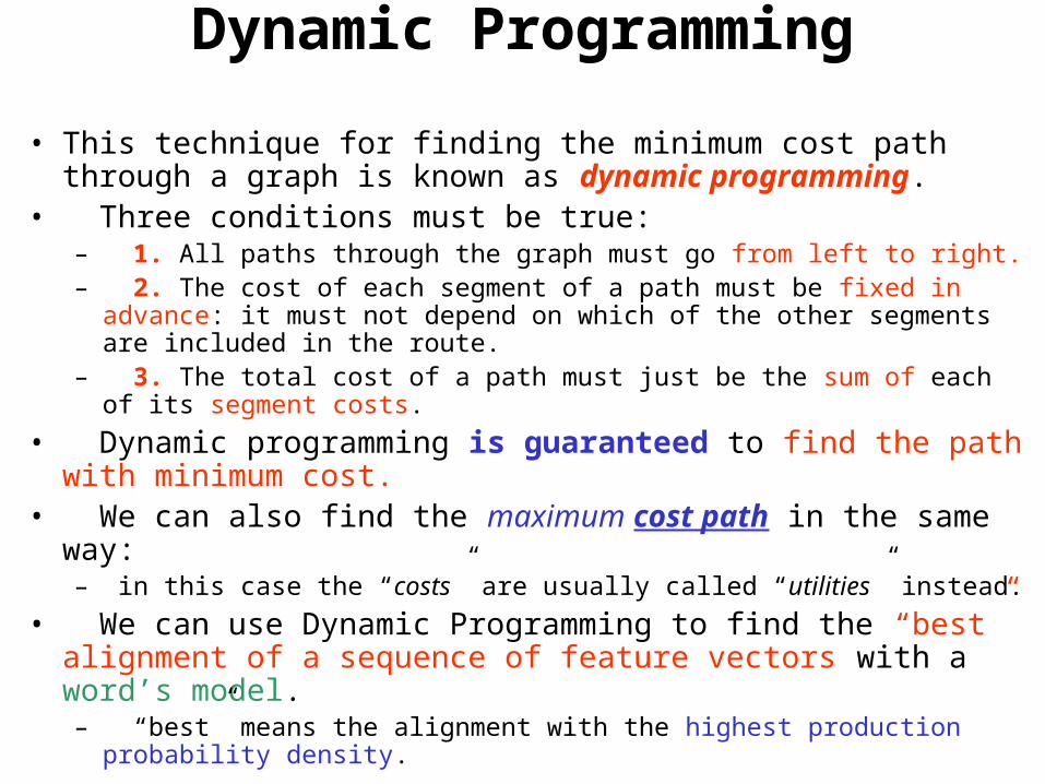
Dynamic Programming

• This technique for finding the minimum cost path through a graph is known as dynamic programming.

• Three conditions must be true:– 1. All paths through the graph must go from left to right.– 2. The cost of each segment of a path must be fixed in advance: it must not

depend on which of the other segments are included in the route.– 3. The total cost of a path must just be the sum of each of its segment costs.

• Dynamic programming is guaranteed to find the path with minimum cost.

• We can also find the maximum cost path in the same way:– in this case the “costs” are usually called “utilities” instead.

• We can use Dynamic Programming to find the “best” alignment of a sequence of feature vectors with a word’s model.– “best” means the alignment with the highest production probability density.

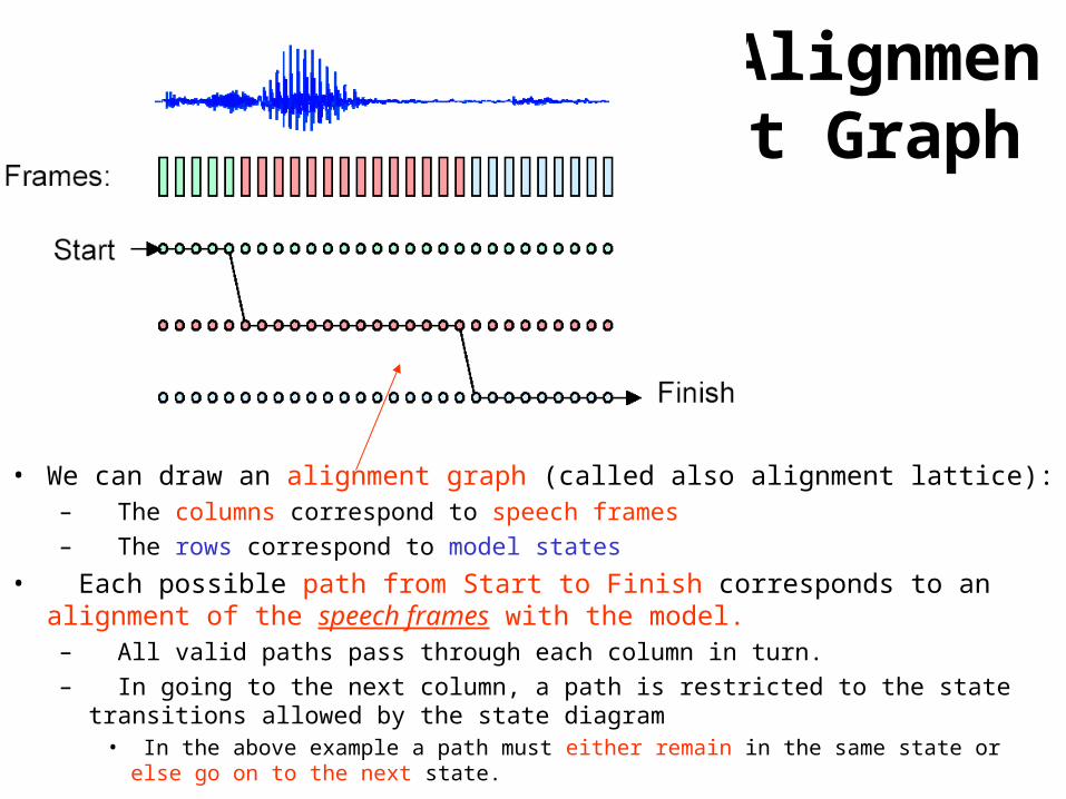
Alignment Graph

• We can draw an alignment graph (called also alignment lattice):– The columns correspond to speech frames

– The rows correspond to model states

• Each possible path from Start to Finish corresponds to an alignment of the speech frames with the model.– All valid paths pass through each column in turn.

– In going to the next column, a path is restricted to the state transitions allowed by the state diagram

• In the above example a path must either remain in the same state or else go on to the next state.

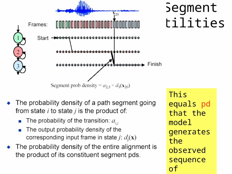
Segment Utilities

This equals pd that the model generates the observed sequence of feature vectors with this particular alignment

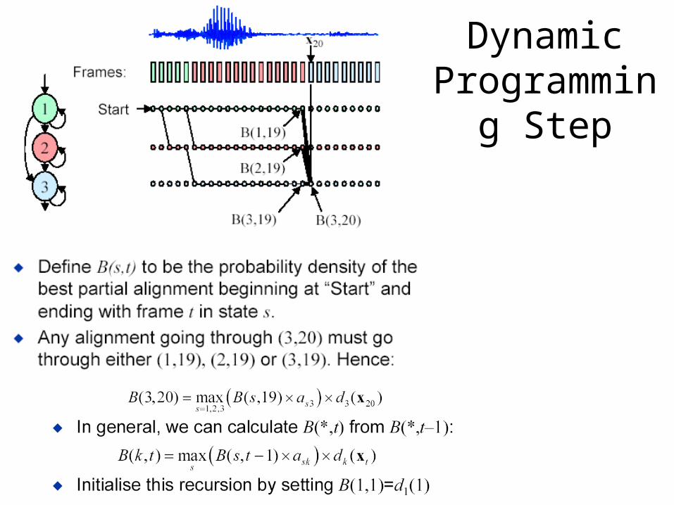
Dynamic Programming

Step

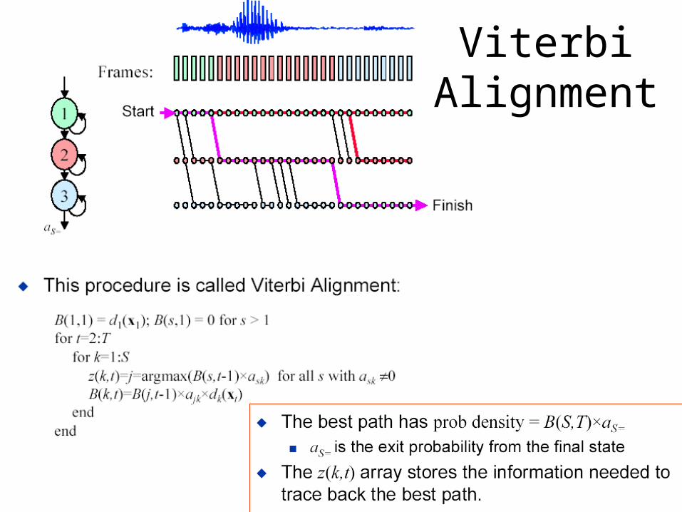
Viterbi Alignment

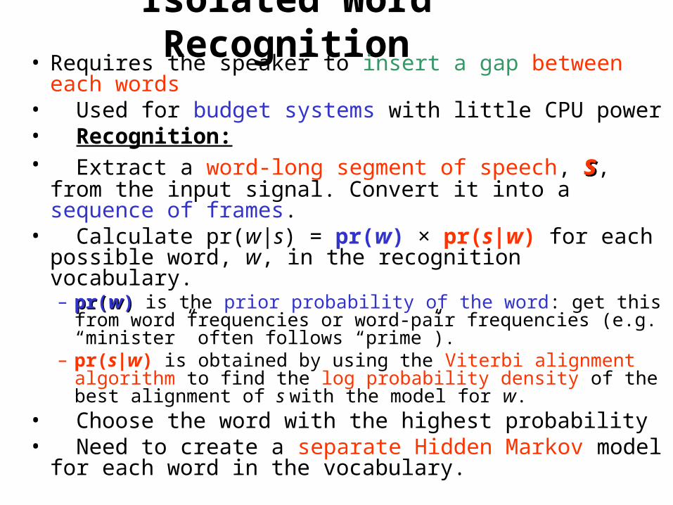
Isolated Word Recognition• Requires the speaker to insert a gap between each words• Used for budget systems with little CPU power• Recognition:• Extract a word-long segment of speech, ss, from the input

signal. Convert it into a sequence of frames.• Calculate pr(w|s) = pr(w) × pr(s|w) for each possible

word, w, in the recognition vocabulary.– pr(pr(ww)) is the prior probability of the word: get this from word

frequencies or word-pair frequencies (e.g. “minister” often follows “prime”).

– pr(s|w) is obtained by using the Viterbi alignment algorithm to find the log probability density of the best alignment of s with the model for w.

• Choose the word with the highest probability• Need to create a separate Hidden Markov model for each

word in the vocabulary.

Applications of HMM

• pattern recognition– genes– Human emotions, persons, gestures,– Spoken natural language recognition, many

levels– Hand-written natural language recognition– Text generation based on writer’s style– Recognition of authorship

Literature

• University Leeds (applets): •

http://www.scs.leeds.ac.uk/scs-only/teaching-materials/HiddenMarkovModels/html_dev/main.html

• Tapas Kanungo (writing recognition) http://www.cfar.umd.edu/~kanungo/

• Rabiner, L. R. 1989. A Tutorial on Hidden Markov Models and Selected Applications in Speech Recognition. Proceedings of the IEEE, Vol. 77, No. 2, pp. 257-286.

• Krogh et al. 1994. J. Mol. Biol. Vol 235, pp.1501-1531.

• Krogh, A. 1998. Salzberg et al In Computational Methods in Molecular Biology. Chap 4.

• Warakagoda, N. D et al MSc thesis online http://jedlik.phy.bme.hu/~gerjanos/HMM/hoved.html

Literature