Hierarchical CPN model-based diagnosis using HAZOP …daedalus.scl.sztaki.hu/pdf/research reports/NemethE.pdf · Hierarchical CPN model-based diagnosis using ... a description of

Hierarchical CPN model-based diagnosis

using HAZOP knowledge

E. Németh, R. Lakner, K. M. Hangos, I. T. Cameron

Research Report SCL-009/2003

Research Report SCL-009/2003 1

Contents

1 Introduction 3

2 Coloured Petri nets (CPNs) 42.1 Coloured Petri nets . . . . . . . . . . . . . . . . . . . . . . . . . . . . . . . . . . . . . . 4

2.1.1 Reachability/Occurrence graph . . . . . . . . . . . . . . . . . . . . . . . . . . . 52.2 Hierarchical coloured Petri nets . . . . . . . . . . . . . . . . . . . . . . . . . . . . . . . 6

2.2.1 Introduction to hierarchical coloured Petri nets . . . . . . . . . . . . . . . . . . 62.2.2 Formal definition of hierarchical coloured Petri nets . . . . . . . . . . . . . . . . 7

2.3 Example for coloured Petri net . . . . . . . . . . . . . . . . . . . . . . . . . . . . . . . 92.4 Example for hierarchical coloured Petri net . . . . . . . . . . . . . . . . . . . . . . . . 11

3 Multi-scale coloured Petri net models of process systems 133.1 Process models . . . . . . . . . . . . . . . . . . . . . . . . . . . . . . . . . . . . . . . . 13

3.1.1 The structure of process models . . . . . . . . . . . . . . . . . . . . . . . . . . . 143.2 Modelling hierarchy . . . . . . . . . . . . . . . . . . . . . . . . . . . . . . . . . . . . . 143.3 The conversion method from hierarchical process models to hierarchical CPN . . . . . 16

4 Goal hierarchy 164.1 Goal-tree construction . . . . . . . . . . . . . . . . . . . . . . . . . . . . . . . . . . . . 174.2 Connection between modelling and goal hierarchies: the functions . . . . . . . . . . . . 17

5 Case study: A tank reactor with cooling jacket 195.1 The description of the tank reactor with cooling jacket . . . . . . . . . . . . . . . . . . 19

5.1.1 Dynamic model equations . . . . . . . . . . . . . . . . . . . . . . . . . . . . . . 195.1.2 Modelling hierarchy . . . . . . . . . . . . . . . . . . . . . . . . . . . . . . . . . 215.1.3 Goal hierarchy . . . . . . . . . . . . . . . . . . . . . . . . . . . . . . . . . . . . 225.1.4 Connection between the modelling and goal hierarchies . . . . . . . . . . . . . . 22

6 Conclusion and future work 23

List of Figures

1 CPN model of the Simple Protocol . . . . . . . . . . . . . . . . . . . . . . . . . . . . . 92 Partial occurrence graph of the of the Simple Protocol . . . . . . . . . . . . . . . . . . 123 The hierarchy of the Simple Protocol . . . . . . . . . . . . . . . . . . . . . . . . . . . . 12

3.a The hierarchical connections of subnets . . . . . . . . . . . . . . . . . . . . . . . 123.b The top level of Simple Protocol . . . . . . . . . . . . . . . . . . . . . . . . . . . 12

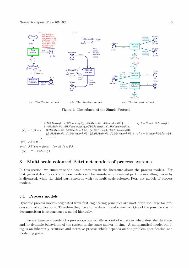
4 The subnets of the Simple Protocol . . . . . . . . . . . . . . . . . . . . . . . . . . . . . 134.a The Sender subnet . . . . . . . . . . . . . . . . . . . . . . . . . . . . . . . . . . . 134.b The Receiver subnet . . . . . . . . . . . . . . . . . . . . . . . . . . . . . . . . . . 134.c The Network subnet . . . . . . . . . . . . . . . . . . . . . . . . . . . . . . . . . . 13

5 An example for flowsheet and sub-flowsheet . . . . . . . . . . . . . . . . . . . . . . . . 166 An example for goal tree . . . . . . . . . . . . . . . . . . . . . . . . . . . . . . . . . . . 177 An example for the connection between the modelling and goal hierarchies with symptoms 198 The diagram of the reactor . . . . . . . . . . . . . . . . . . . . . . . . . . . . . . . . . 199 The modelling hierarchy of the reactor . . . . . . . . . . . . . . . . . . . . . . . . . . . 2110 The modelling hierarchy represented by hierarchical CPN of the reactor . . . . . . . . 2211 The goal hierarchy of the reactor . . . . . . . . . . . . . . . . . . . . . . . . . . . . . . 2212 The connection between the modelling and goal hierarchies with symptoms in the reactor

model . . . . . . . . . . . . . . . . . . . . . . . . . . . . . . . . . . . . . . . . . . . . . 23


Hierarchical CPN model-based diagnosis using HAZOP knowledge

Erzsébet Németh Rozália LaknerDepartment of Computer Science Department of Computer Science

University of Veszprém University of VeszprémH-8201 Veszprém, P.O. Box 158, Hungary H-8201 Veszprém, P.O. Box 158, Hungary

E-mail: [email protected] E-mail: [email protected]

Katalin M. Hangos Ian T. CameronSystems and Control Research Laboratory Department of Chemical EngineeringComputer and Automation Institute HAS The University of QueenslandH-1518 Budapest, P.O. Box 63, Hungary Australia

E-mail: [email protected] E-mail: [email protected]

Abstract

The multi-scale modelling of process systems using hierarchical coloured Petri nets for diag-

nostics is investigated in this report. A case study is used to systematically show the modelling

approach using an illustrative example of a tank reactor with cooling jacket. This form of repre-

sentation shows how CPNs can provide a hierarchically structured framework for advanced fault

diagnosis.


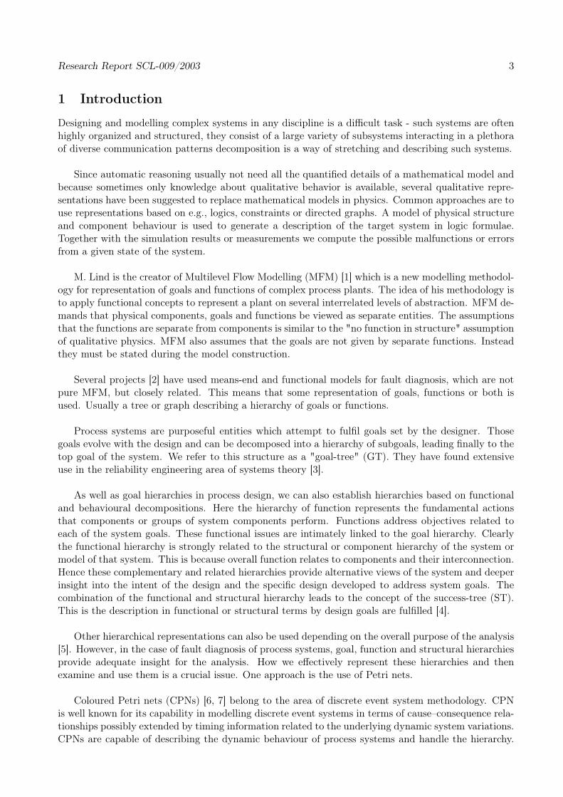
1 Introduction

Designing and modelling complex systems in any discipline is a difficult task - such systems are oftenhighly organized and structured, they consist of a large variety of subsystems interacting in a plethoraof diverse communication patterns decomposition is a way of stretching and describing such systems.

Since automatic reasoning usually not need all the quantified details of a mathematical model andbecause sometimes only knowledge about qualitative behavior is available, several qualitative repre-sentations have been suggested to replace mathematical models in physics. Common approaches are touse representations based on e.g., logics, constraints or directed graphs. A model of physical structureand component behaviour is used to generate a description of the target system in logic formulae.Together with the simulation results or measurements we compute the possible malfunctions or errorsfrom a given state of the system.

M. Lind is the creator of Multilevel Flow Modelling (MFM) [1] which is a new modelling methodol-ogy for representation of goals and functions of complex process plants. The idea of his methodology isto apply functional concepts to represent a plant on several interrelated levels of abstraction. MFM de-mands that physical components, goals and functions be viewed as separate entities. The assumptionsthat the functions are separate from components is similar to the "no function in structure" assumptionof qualitative physics. MFM also assumes that the goals are not given by separate functions. Insteadthey must be stated during the model construction.

Several projects [2] have used means-end and functional models for fault diagnosis, which are notpure MFM, but closely related. This means that some representation of goals, functions or both isused. Usually a tree or graph describing a hierarchy of goals or functions.

Process systems are purposeful entities which attempt to fulfil goals set by the designer. Thosegoals evolve with the design and can be decomposed into a hierarchy of subgoals, leading finally to thetop goal of the system. We refer to this structure as a "goal-tree" (GT). They have found extensiveuse in the reliability engineering area of systems theory [3].

As well as goal hierarchies in process design, we can also establish hierarchies based on functionaland behavioural decompositions. Here the hierarchy of function represents the fundamental actionsthat components or groups of system components perform. Functions address objectives related toeach of the system goals. These functional issues are intimately linked to the goal hierarchy. Clearlythe functional hierarchy is strongly related to the structural or component hierarchy of the system ormodel of that system. This is because overall function relates to components and their interconnection.Hence these complementary and related hierarchies provide alternative views of the system and deeperinsight into the intent of the design and the specific design developed to address system goals. Thecombination of the functional and structural hierarchy leads to the concept of the success-tree (ST).This is the description in functional or structural terms by design goals are fulfilled [4].

Other hierarchical representations can also be used depending on the overall purpose of the analysis[5]. However, in the case of fault diagnosis of process systems, goal, function and structural hierarchiesprovide adequate insight for the analysis. How we effectively represent these hierarchies and thenexamine and use them is a crucial issue. One approach is the use of Petri nets.

Coloured Petri nets (CPNs) [6, 7] belong to the area of discrete event system methodology. CPNis well known for its capability in modelling discrete event systems in terms of cause–consequence rela-tionships possibly extended by timing information related to the underlying dynamic system variations.CPNs are capable of describing the dynamic behaviour of process systems and handle the hierarchy.


The basic idea behind using hierarchical CPNs is to allow the modeller to construct a large model byusing a number of small CPNs which are related to each other in a well-defined way.

This report is organized as follows. First the representation tool of multi-scale process models,coloured Petri net with hierarchical extension is described with its properties. Thereafter the multi-scale models of process systems with modelling and goal hierarchies are discussed for diagnosis. Thedescribed representation is shown in a tank reactor with cooling jacket. Finally conclusions are drawn.

2 Coloured Petri nets (CPNs)

In this section, we summarize the basic notations found in the literature about coloured Petri netsand hierarchical coloured Petri nets. For first, the general coloured case will be considered, while thesecond part concerns with the hierarchical Petri nets.

2.1 Coloured Petri nets

Coloured Petri nets (CPNs) [8] belong to the area of discrete event system methodology. A CPN iswell known for its capability in modelling discrete event systems.

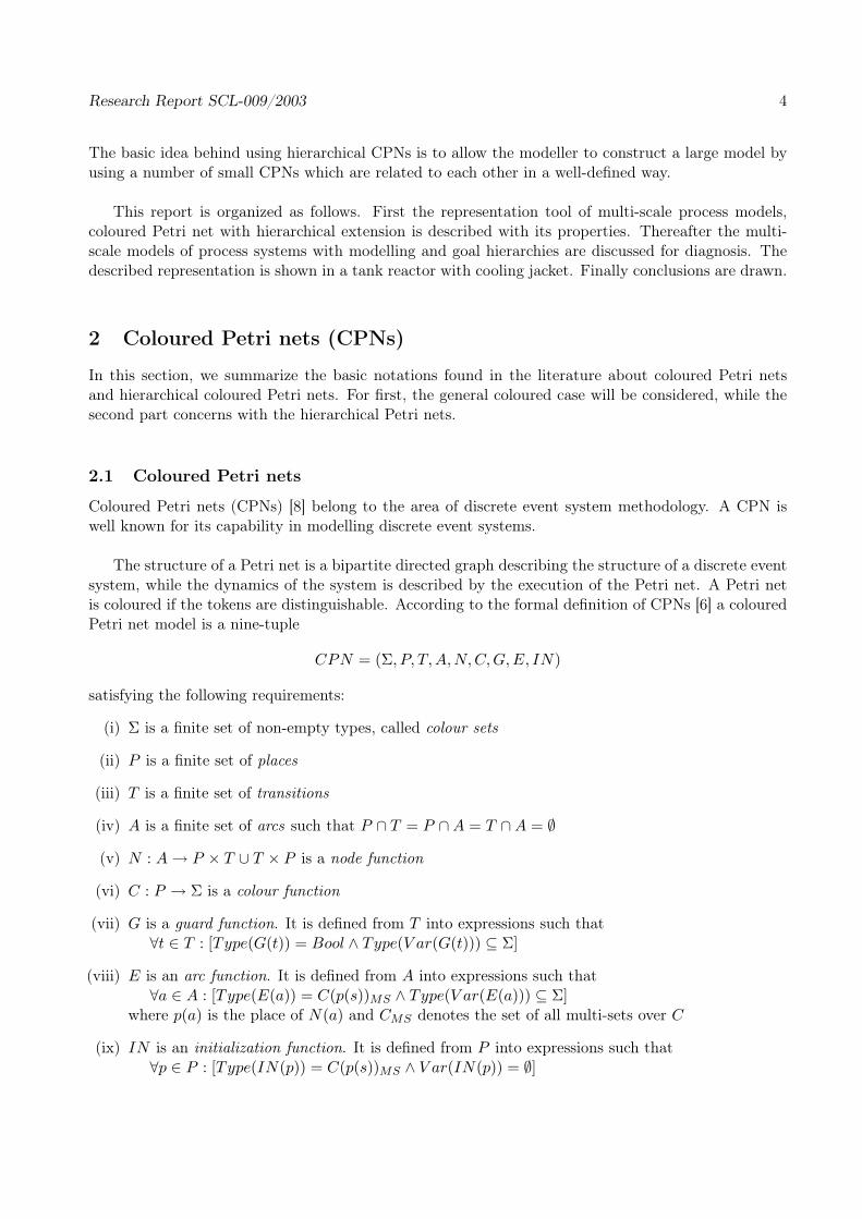
The structure of a Petri net is a bipartite directed graph describing the structure of a discrete eventsystem, while the dynamics of the system is described by the execution of the Petri net. A Petri netis coloured if the tokens are distinguishable. According to the formal definition of CPNs [6] a colouredPetri net model is a nine-tuple

CPN = (Σ, P, T, A, N, C, G, E, IN)

satisfying the following requirements:

(i) Σ is a finite set of non-empty types, called colour sets

(ii) P is a finite set of places

(iii) T is a finite set of transitions

(iv) A is a finite set of arcs such that P ∩ T = P ∩ A = T ∩ A = ∅

(v) N : A → P × T ∪ T × P is a node function

(vi) C : P → Σ is a colour function

(vii) G is a guard function. It is defined from T into expressions such that∀t ∈ T : [Type(G(t)) = Bool ∧ Type(V ar(G(t))) ⊆ Σ]

(viii) E is an arc function. It is defined from A into expressions such that∀a ∈ A : [Type(E(a)) = C(p(s))MS ∧ Type(V ar(E(a))) ⊆ Σ]

where p(a) is the place of N(a) and CMS denotes the set of all multi-sets over C

(ix) IN is an initialization function. It is defined from P into expressions such that∀p ∈ P : [Type(IN(p)) = C(p(s))MS ∧ V ar(IN(p)) = ∅]


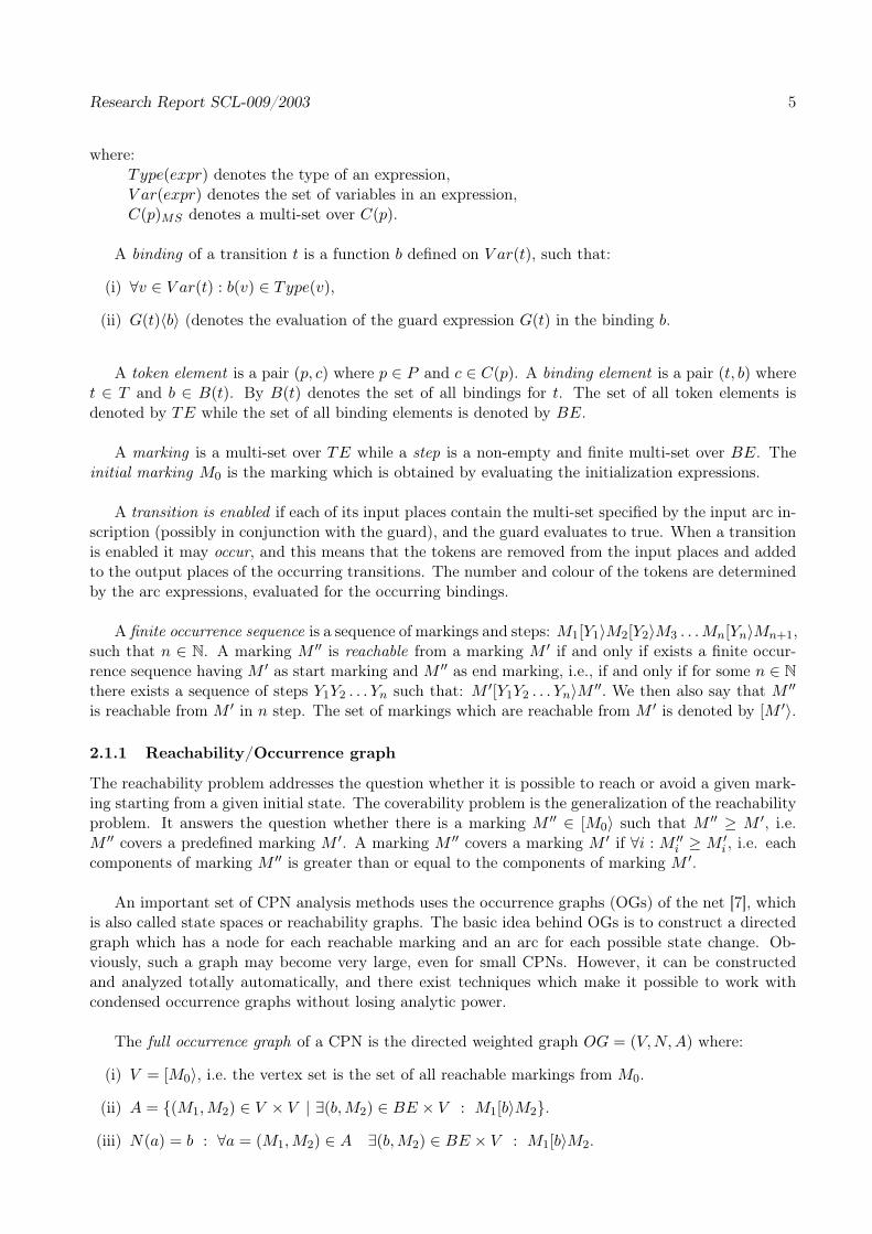
where:Type(expr) denotes the type of an expression,V ar(expr) denotes the set of variables in an expression,C(p)MS denotes a multi-set over C(p).

A binding of a transition t is a function b defined on V ar(t), such that:

(i) ∀v ∈ V ar(t) : b(v) ∈ Type(v),

(ii) G(t)〈b〉 (denotes the evaluation of the guard expression G(t) in the binding b.

A token element is a pair (p, c) where p ∈ P and c ∈ C(p). A binding element is a pair (t, b) wheret ∈ T and b ∈ B(t). By B(t) denotes the set of all bindings for t. The set of all token elements isdenoted by TE while the set of all binding elements is denoted by BE.

A marking is a multi-set over TE while a step is a non-empty and finite multi-set over BE. Theinitial marking M0 is the marking which is obtained by evaluating the initialization expressions.

A transition is enabled if each of its input places contain the multi-set specified by the input arc in-scription (possibly in conjunction with the guard), and the guard evaluates to true. When a transitionis enabled it may occur, and this means that the tokens are removed from the input places and addedto the output places of the occurring transitions. The number and colour of the tokens are determinedby the arc expressions, evaluated for the occurring bindings.

A finite occurrence sequence is a sequence of markings and steps: M1[Y1〉M2[Y2〉M3 . . . Mn[Yn〉Mn+1,such that n ∈ N. A marking M ′′ is reachable from a marking M ′ if and only if exists a finite occur-rence sequence having M ′ as start marking and M ′′ as end marking, i.e., if and only if for some n ∈ N

there exists a sequence of steps Y1Y2 . . . Yn such that: M ′[Y1Y2 . . . Yn〉M′′. We then also say that M ′′

is reachable from M ′ in n step. The set of markings which are reachable from M ′ is denoted by [M ′〉.

2.1.1 Reachability/Occurrence graph

The reachability problem addresses the question whether it is possible to reach or avoid a given mark-ing starting from a given initial state. The coverability problem is the generalization of the reachabilityproblem. It answers the question whether there is a marking M ′′ ∈ [M0〉 such that M ′′ ≥ M ′, i.e.M ′′ covers a predefined marking M ′. A marking M ′′ covers a marking M ′ if ∀i : M ′′

i ≥ M ′

i , i.e. eachcomponents of marking M ′′ is greater than or equal to the components of marking M ′.

An important set of CPN analysis methods uses the occurrence graphs (OGs) of the net [7], whichis also called state spaces or reachability graphs. The basic idea behind OGs is to construct a directedgraph which has a node for each reachable marking and an arc for each possible state change. Ob-viously, such a graph may become very large, even for small CPNs. However, it can be constructedand analyzed totally automatically, and there exist techniques which make it possible to work withcondensed occurrence graphs without losing analytic power.

The full occurrence graph of a CPN is the directed weighted graph OG = (V, N, A) where:

(i) V = [M0〉, i.e. the vertex set is the set of all reachable markings from M0.

(ii) A = {(M1, M2) ∈ V × V | ∃(b, M2) ∈ BE × V : M1[b〉M2}.

(iii) N(a) = b : ∀a = (M1, M2) ∈ A ∃(b, M2) ∈ BE × V : M1[b〉M2.


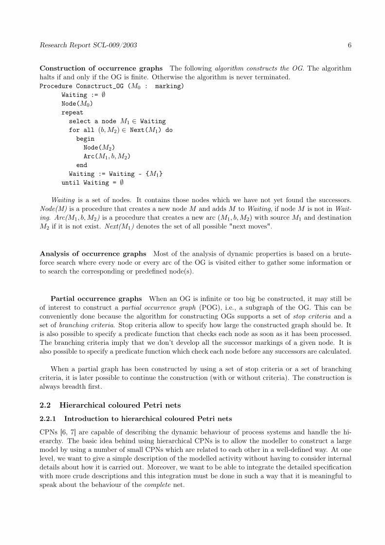
Construction of occurrence graphs The following algorithm constructs the OG. The algorithmhalts if and only if the OG is finite. Otherwise the algorithm is never terminated.Procedure Consctruct_OG (M0 : marking)

Waiting := ∅Node(M0)

repeat

select a node M1 ∈ Waiting

for all (b, M2) ∈ Next(M1) do

begin

Node(M2)

Arc(M1, b, M2)

end

Waiting := Waiting - {M1}

until Waiting = ∅

Waiting is a set of nodes. It contains those nodes which we have not yet found the successors.Node(M) is a procedure that creates a new node M and adds M to Waiting, if node M is not in Wait-ing. Arc(M1, b, M2) is a procedure that creates a new arc (M1, b, M2) with source M1 and destinationM2 if it is not exist. Next(M1) denotes the set of all possible "next moves".

Analysis of occurrence graphs Most of the analysis of dynamic properties is based on a brute-force search where every node or every arc of the OG is visited either to gather some information orto search the corresponding or predefined node(s).

Partial occurrence graphs When an OG is infinite or too big be constructed, it may still beof interest to construct a partial occurrence graph (POG), i.e., a subgraph of the OG. This can beconveniently done because the algorithm for constructing OGs supports a set of stop criteria and aset of branching criteria. Stop criteria allow to specify how large the constructed graph should be. Itis also possible to specify a predicate function that checks each node as soon as it has been processed.The branching criteria imply that we don’t develop all the successor markings of a given node. It isalso possible to specify a predicate function which check each node before any successors are calculated.

When a partial graph has been constructed by using a set of stop criteria or a set of branchingcriteria, it is later possible to continue the construction (with or without criteria). The construction isalways breadth first.

2.2 Hierarchical coloured Petri nets

2.2.1 Introduction to hierarchical coloured Petri nets

CPNs [6, 7] are capable of describing the dynamic behaviour of process systems and handle the hi-erarchy. The basic idea behind using hierarchical CPNs is to allow the modeller to construct a largemodel by using a number of small CPNs which are related to each other in a well-defined way. At onelevel, we want to give a simple description of the modelled activity without having to consider internaldetails about how it is carried out. Moreover, we want to be able to integrate the detailed specificationwith more crude descriptions and this integration must be done in such a way that it is meaningful tospeak about the behaviour of the complete net.


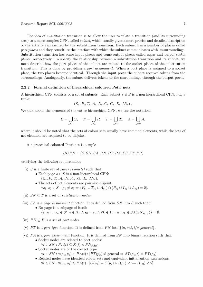
The idea of substitution transition is to allow the user to relate a transition (and its surroundingarcs) to a more complex CPN, called subnet, which usually gives a more precise and detailed descriptionof the activity represented by the substitution transition. Each subnet has a number of places calledport places and they constitute the interface with which the subnet communicates with its surroundings.Substitution transition has some input places and some output places called input and output socketplaces, respectively. To specify the relationship between a substitution transition and its subnet, wemust describe how the port places of the subnet are related to the socket places of the substitutiontransition. This is done by providing a port assignment. When a port place is assigned to a socketplace, the two places become identical. Through the input ports the subnet receives tokens from thesurroundings. Analogously, the subnet delivers tokens to the surroundings through the output ports.

2.2.2 Formal definition of hierarchical coloured Petri nets

A hierarchical CPN consists of a set of subnets. Each subnet s ∈ S is a non-hierarchical CPN, i.e., atuple:

(Σs, Ps, Ts, As, Ns, Cs, Gs, Es, INs) .

We talk about the elements of the entire hierarchical CPN, we use the notation:

Σ =⋃

s∈S

Σs P =⋃

s∈S

Ps T =⋃

s∈S

Ts A =⋃

s∈S

As

where it should be noted that the sets of colour sets usually have common elements, while the sets ofnet elements are required to be disjoint.

A hierarchical coloured Petri-net is a tuple

HCPN = (S, SN, SA, PN, PT, PA, FS, FT, PP )

satisfying the following requirements:

(i) S is a finite set of pages (subnets) such that:• Each page s ∈ S is a non-hierarchical CPN:

(Σs, Ps, Ts, As, Ns, Cs, Gs, Es, INs).• The sets of net elements are pairwise disjoint:

∀s1, s2 ∈ S : [s1 6= s2 ⇒ (Ps1∪ Ts1

∪ As1) ∩ (Ps2

∪ Ts2∪ As2

) = ∅].

(ii) SN ⊆ T is a set of substitution nodes.

(iii) SA is a page assignment function. It is defined from SN into S such that:• No page is a subpage of itself:

{s0s1 . . . sn ∈ S∗|n ∈ N+ ∧ s0 = sn ∧ ∀k ∈ 1 . . . n : sk ∈ SA(SNsk−1)} = ∅.

(iv) PN ⊆ P is a set of port nodes.

(v) PT is a port type function. It is defined from PN into {in, out, i/o, general}.

(vi) PA is a port assignment function. It is defined from SN into binary relation such that:• Socket nodes are related to port nodes:

∀t ∈ SN : PA(t) ⊆ X(t) × PNSA(t).• Socket nodes are of the correct type:

∀t ∈ SN : ∀(p1, p2) ∈ PA(t) : [PT (p2) 6= general ⇒ ST (p1, t) = PT (p2)].• Related nodes have identical colour sets and equivalent initialization expressions:

∀t ∈ SN : ∀(p1, p2) ∈ PA(t) : [C(p1) = C(p2) ∧ I(p1) <>= I(p2) <>].


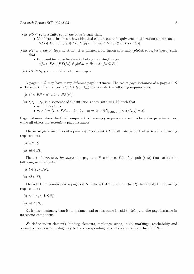
(vii) FS ⊆ Ps is a finite set of fusion sets such that:• Members of fusion set have identical colour sets and equivalent initialization expressions:

∀fs ∈ FS : ∀p1, p2 ∈ fs : [C(p1) = C(p2) ∧ I(p1) <>= I(p2) <>].

(viii) FT is a fusion type function. It is defined from fusion sets into {global, page, instance} suchthat:

• Page and instance fusion sets belong to a single page:∀fs ∈ FS : [FT (fs) 6= global ⇒ ∃s ∈ S : fs ⊆ Ps].

(ix) PP ∈ SMS is a multi-set of prime pages.

A page s ∈ S may have many different page instances. The set of page instances of a page s ∈ Sis the set SIs of all triples (s∗, n∗, t1t2 . . . tm) that satisfy the following requirements:

(i) s∗ ∈ PP ∧ n∗ ∈ 1 . . . PP (s∗).

(ii) t1t2 . . . tm is a sequence of substitution nodes, with m ∈ N, such that:• m = 0 ⇒ s∗ = s• m > 0 ⇒ (t1 ∈ SNs∗ ∧ [k ∈ 2 . . . m ⇒ tk ∈ SNSA(tk−1)] ∧ SA(tm) = s).

Page instances where the third component is the empty sequence are said to be prime page instances,while all others are secondary page instances.

The set of place instances of a page s ∈ S is the set PIs of all pair (p, id) that satisfy the followingrequirements:

(i) p ∈ Ps.

(ii) id ∈ SIs.

The set of transition instances of a page s ∈ S is the set TIs of all pair (t, id) that satisfy thefollowing requirements:

(i) t ∈ Ts \ SNs.

(ii) id ∈ SIs.

The set of arc instances of a page s ∈ S is the set AIs of all pair (a, id) that satisfy the followingrequirements:

(i) a ∈ As \ A(SNs).

(ii) id ∈ SIs.

Each place instance, transition instance and arc instance is said to belong to the page instance inits second component.

We define token elements, binding elements, markings, steps, initial markings, reachability andoccurrence sequences analogously to the corresponding concepts for non-hierarchical CPNs.


2.3 Example for coloured Petri net

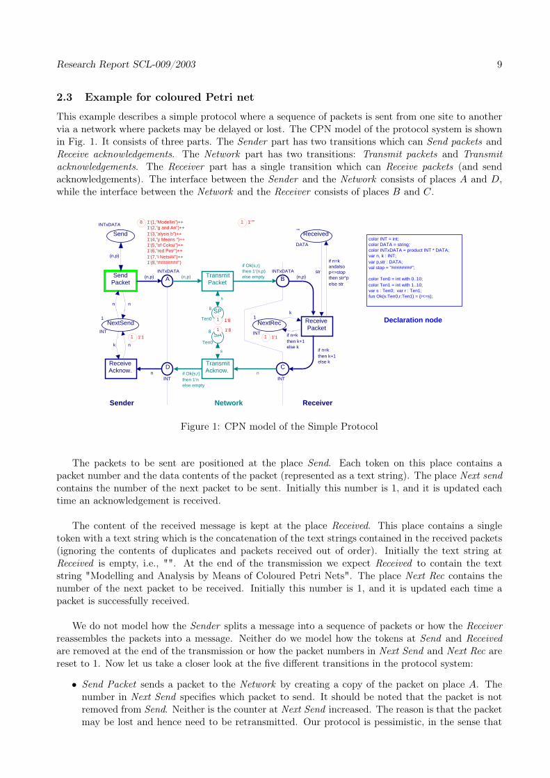
This example describes a simple protocol where a sequence of packets is sent from one site to anothervia a network where packets may be delayed or lost. The CPN model of the protocol system is shownin Fig. 1. It consists of three parts. The Sender part has two transitions which can Send packets andReceive acknowledgements. The Network part has two transitions: Transmit packets and Transmitacknowledgements. The Receiver part has a single transition which can Receive packets (and sendacknowledgements). The interface between the Sender and the Network consists of places A and D,while the interface between the Network and the Receiver consists of places B and C.

color INT = int;color DATA = string; color INTxDATA = product INT * DATA;var n, k : INT;var p,str : DATA;val stop = "########";

color Ten0 = int with 0..10;color Ten1 = int with 1..10;var s : Ten0; var r : Ten1;fun Ok(s:Ten0,r:Ten1) = (r<=s);

SendPacket

TransmitPacket

ReceivePacket

ReceiveAcknow.

TransmitAcknow.

Send

INTxDATA 8 1‘(1,"Modellin")++ 1‘(2,"g and An")++ 1‘(3,"alysis b")++ 1‘(4,"y Means ")++ 1‘(5,"of Colou")++ 1‘(6,"red Petr")++ 1‘(7,"i Nets##")++ 1‘(8,"########")

NextSendINT

1

1 1‘1

D

INT

AINTxDATA

Received

DATA

1 1‘""

""

NextRec

INT

1

1 1‘1

BINTxDATA

C

INT

Sender Network Receiver

SP8

Ten0 1 1‘8

SA1 1‘8

Ten0

8

Declaration node

(n,p) (n,p)

if Ok(s,r)then 1‘(n,p)else empty

(n,p)

(n,p)

if n=kandalsop<>stopthen str^pelse str

if n=kthen k+1else k

n

k


if Ok(s,r)then 1‘nelse empty

n

k n

n n

str

s

s

Figure 1: CPN model of the Simple Protocol

The packets to be sent are positioned at the place Send. Each token on this place contains apacket number and the data contents of the packet (represented as a text string). The place Next sendcontains the number of the next packet to be sent. Initially this number is 1, and it is updated eachtime an acknowledgement is received.

The content of the received message is kept at the place Received. This place contains a singletoken with a text string which is the concatenation of the text strings contained in the received packets(ignoring the contents of duplicates and packets received out of order). Initially the text string atReceived is empty, i.e., "". At the end of the transmission we expect Received to contain the textstring "Modelling and Analysis by Means of Coloured Petri Nets". The place Next Rec contains thenumber of the next packet to be received. Initially this number is 1, and it is updated each time apacket is successfully received.

We do not model how the Sender splits a message into a sequence of packets or how the Receiverreassembles the packets into a message. Neither do we model how the tokens at Send and Receivedare removed at the end of the transmission or how the packet numbers in Next Send and Next Rec arereset to 1. Now let us take a closer look at the five different transitions in the protocol system:

• Send Packet sends a packet to the Network by creating a copy of the packet on place A. Thenumber in Next Send specifies which packet to send. It should be noted that the packet is notremoved from Send. Neither is the counter at Next Send increased. The reason is that the packetmay be lost and hence need to be retransmitted. Our protocol is pessimistic, in the sense that


it continues to repeat the same packet - until it gets an acknowledgment telling that the packethas been successfully received.

• Transmit Packet transmits a packet from the Sender site of the Network to the Receiver siteby moving the corresponding token from A to B. The boolean expression Ok(s, r) determineswhether the packet is successfully transmitted or lost. The variable r will be bound to an arbitraryvalue in its colour set (i.e., to any integer between 1 and 10). Design/CPN makes a fair choicebetween the 10 values (provided that fair simulation is chosen in General Simulation Options).The Ok function returns true if the value of r is less than or equal to the value of s. This meansthat the probability of successful transmission is determined by the token at place SP . We havegiven SP a token with value 8. Hence we have 80% chance for successful transmission. However,it is easy to modify the success rate, simply by changing the token value at SP .

• Receive Packet receives a packet and checks whether the packet number n is identical to thenumber k in Next Rec. When the two numbers match, the number in Next Rec is increased by1 and the text string in the packet is concatenated to the text string in Received - unless it isstop = ”########”, which by convention indicates end-of-message. Otherwise, the packetis ignored and the number in Next Rec 4 is left unchanged. In both cases an acknowledgment issent containing the number of the next packet which the Sender should send.

• Transmit Acknowledgement transmits an acknowledgment from the Receiver site of the Networkto the Sender site by moving the corresponding token from C to D. The transition works ina similar way as Transmit Packet. This means that the acknowledgment may be lost, with aprobability determined by the token at place SA.

• Receive Acknowledgment receives an acknowledgment and updates the number in Next Send byreplacing the old value with the one contained in the acknowledgment. After a number of stepsthe CPN may have reached the intermediate marking shown in Fig X.

The CPN from Fig. 1 represented as a many-tuple:

(i) Σ = {INT, DATA, INT × DATA, Ten0, T en1}

(ii) P = {Send, Next Send, Received, Next Rec, A, B, C, D, SP, SA}

(iii) T = {Send Packet, Receive Acknow., Transmit Packet, T ransmitAcknow., ReceivePacket}

(iv) A = {Send_TO_Send Packet, Next Send_TO_Send Packet,Send Packet_TO_Send, Send Packet_TO_A, Send Packet_TO_Next Send,Next Send_TO_Receive Acknow., D_TO_Receive Acknow.,Receive Acknow._TO_Next Send,A_TO_Transmit Packet, SP_TO_Transmit Packet,T ransmit Packet_TO_SP, Transmit Packet_TO_B,C_TO_Transmit Acknow., SA_TO_Transmit Acknow.,Transmit Acknow._TO_SA, Transmit Acknow._TO_D,Received_TO_Received Packet, B_TO_Received Packet, Next Rec_TO_Received Packet,Received Packet_TO_Next Rec, Received Packet_TO_C, Received Packet_TO_Received}

(v) N(a) = (SOURCE, DEST ) if a is in the form SOURCE_TO_DEST

(vi) C(p) =

INT if p ∈ {Next Send, D, C, Next Rec}DATA if p = ReceivedINT × DATA if p ∈ {Send, A, B}Ten0 if p ∈ {SA, SP}.

(vii) G(t) = true if t ∈ T


(viii) E(a) =

(n, p) if a ∈ {Send_TO_Send Packet, Send Packet_TO_Send,Send Packet_TO_A, A_TO_Transmit Packet, B_TO_Received Packet}

n if a ∈ {Next Send_TO_Send Packet, Send Packet_TO_Next Send,Receive Acknow._TO_Next Send, D_TO_Receive Acknow.,C_TO_Transmit Acknow.}

k if a ∈ {Next Send_TO_Receive Acknow., Next Rec_TO_Received Packet}s if a ∈ {SP_TO_Transmit Packet, T ransmit Packet_TO_SP,

SA_TO_Transmit Acknow., Transmit Acknow._TO_SA}str if a = Received_TO_Received Packetif Ok(s, r)

then 1‘nelse empty if a = Transmit Acknow._TO_D

if Ok(s, r)then 1‘(n, p)else empty if a = Transmit Packet_TO_B

if n = kthen k + 1else k if a ∈ {Received Packet_TO_Next Rec, Received Packet_TO_C}

if n = kandalso p <> stopthen str∧pelse str if a = Received Packet_TO_Received.

(ix) I(p) =

1‘(1, ”Modellin”)++1‘(2, ”g and An”)++

1‘(3, ”alysis b”)++1‘(4, ”y Means”)++

1‘(5, ”of Colou”)++1‘(6, ”red Petr”)++

1‘(7, ”i Nets##”)++1‘(8, ”########”) if p = Send1‘1 if p = Next Send1‘8 if p = SA1‘8 if p = SP1‘1 if p = Next Rec1‘”” if p = Received∅ if otherwise.

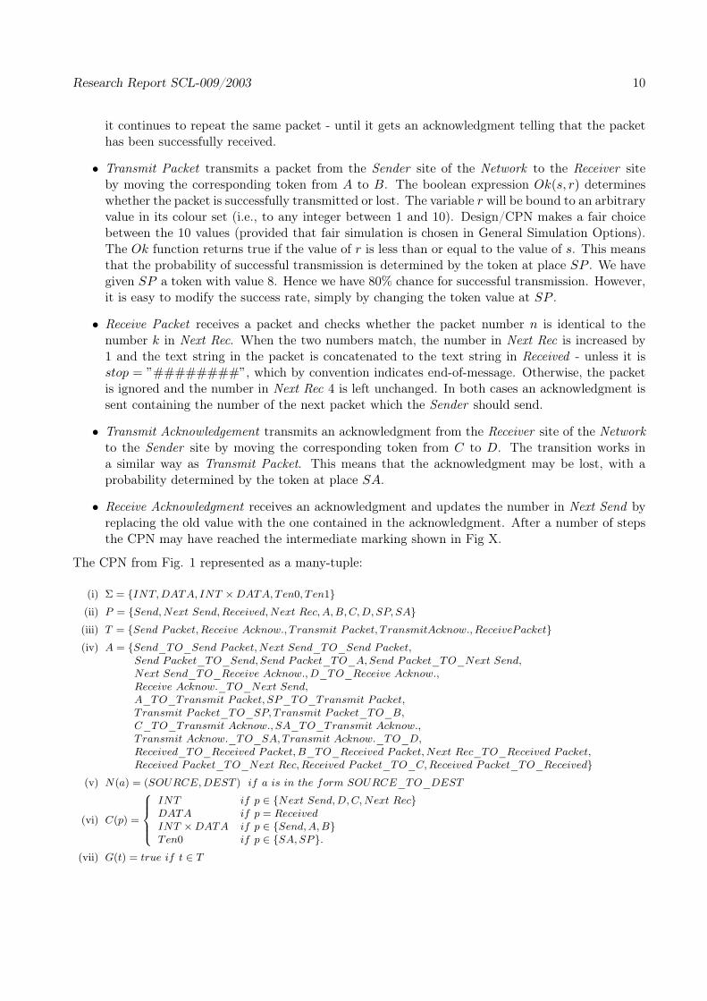
The example for partial occurrence graph can be seen in Fig. 2.

2.4 Example for hierarchical coloured Petri net

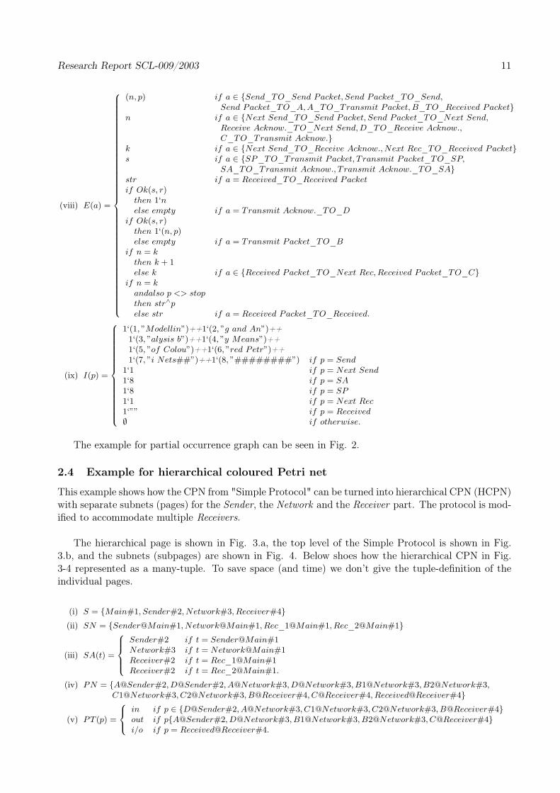
This example shows how the CPN from "Simple Protocol" can be turned into hierarchical CPN (HCPN)with separate subnets (pages) for the Sender, the Network and the Receiver part. The protocol is mod-ified to accommodate multiple Receivers.

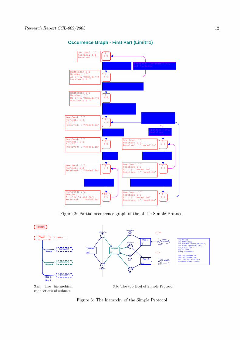
The hierarchical page is shown in Fig. 3.a, the top level of the Simple Protocol is shown in Fig.3.b, and the subnets (subpages) are shown in Fig. 4. Below shoes how the hierarchical CPN in Fig.3-4 represented as a many-tuple. To save space (and time) we don’t give the tuple-definition of theindividual pages.

(i) S = {Main#1, Sender#2, Network#3, Receiver#4}

(ii) SN = {Sender@Main#1, Network@Main#1, Rec_1@Main#1, Rec_2@Main#1}

(iii) SA(t) =

Sender#2 if t = Sender@Main#1Network#3 if t = Network@Main#1Receiver#2 if t = Rec_1@Main#1Receiver#2 if t = Rec_2@Main#1.

(iv) PN = {A@Sender#2, D@Sender#2, A@Network#3, D@Network#3, B1@Network#3, B2@Network#3,C1@Network#3, C2@Network#3, B@Receiver#4, C@Receiver#4, Received@Receiver#4}

(v) PT (p) =

in if p ∈ {D@Sender#2, A@Network#3, C1@Network#3, C2@Network#3, B@Receiver#4}out if p{A@Sender#2, D@Network#3, B1@Network#3, B2@Network#3, C@Receiver#4}i/o if p = Received@Receiver#4.


1 1:1

NextSend: 1‘1NextRec: 1‘1Received: 1‘""

2 1:2

NextSend: 1‘1NextRec: 1‘1A: 1‘(1,"Modellin")Received: 1‘""

3 1:1

NextSend: 1‘1NextRec: 1‘1B: 1‘(1,"Modellin")Received: 1‘""

4 2:2

NextSend: 1‘1NextRec: 1‘2C: 1‘2Received: 1‘"Modellin"

5 2:1

NextSend: 1‘1NextRec: 1‘2Received: 1‘"Modellin"

6 1:1

NextSend: 1‘1NextRec: 1‘2D: 1‘2Received: 1‘"Modellin"

8 2:1

NextSend: 1‘2NextRec: 1‘2Received: 1‘"Modellin"

7 1:2

NextSend: 1‘1NextRec: 1‘2A: 1‘(1,"Modellin")Received: 1‘"Modellin"

10 1:2

NextSend: 1‘2NextRec: 1‘2A: 1‘(2,"g and An")Received: 1‘"Modellin"

9 1:1

NextSend: 1‘1NextRec: 1‘2B: 1‘(1,"Modellin")Received: 1‘"Modellin"

Occurrence Graph - First Part (Limit=1)

SendPack: {p="Modellin",n=1}

TranPack: {p="Modellin",n=1,Ok=false}

TranPack: {p="Modellin",n=1,Ok=true}

RecPack: {str="",p="Modellin",n=1,k=1}

TranAck: {n=2,Ok=false}

TranAck: {n=2,Ok=true}

RecAck: {n=2,k=1}

SendPack: {p="Modellin",n=1}

SendPack:{p="g and An",n=2}

TranPack: {p="Modellin",n=1,Ok=true}

RecPack:{str="Modellin",p="Modellin",n=1,k=2}

Figure 2: Partial occurrence graph of the of the Simple Protocol

Top#1 M Prime

Hierarchy#10010

Sender#2

Network#3

Receiver#4

Sender

Network

Rec_1

Rec_2

3.a: The hierarchicalconnections of subnets

color INT = int;color DATA = string; color INTxDATA = product INT * DATA;color INTxINT = product INT * INT;var n, k, n1, n2 : INT;var p,str : DATA;val stop = "########";

color Ten0 = int with 0..10;color Ten1 = int with 1..10;var s : Ten0; var r, r1, r2 : Ten1;fun Ok(s:Ten0,r:Ten1) = (r<=s);

D

INTxINT

AINTxDATA

Received

DATA

1 1‘""

""

B1INTxDATA

C1

INT

Sender

HS

Network

HS

Rec_1

HSB2

INTxDATA

C2

INT

Rec_2

HS

Received

DATA

1 1‘""

""

3.b: The top level of Simple Protocol

Figure 3: The hierarchy of the Simple Protocol


SendPacket

NextSendINT

1

1 1‘1

ReceiveAcknow.

Send

81‘(1,"Modellin")++ 1‘(2,"g and An")++ 1‘(3,"alysis b")++ 1‘(4,"y Means ")++ 1‘(5,"of Colou")++ 1‘(6,"red Petr")++ 1‘(7,"i Nets##")++ 1‘(8,"########")

D

INTxINT

P In

AINTxDATA

P Out

(n,p)

k imin(n1,n2)

n n

(n,p)

1‘(n1,1)++1‘(n2,2)

4.a: The Sender subnet

NextRec

INT

1

1 1‘1

ReceivePacket

C

INT

P Out

Received

DATA

1 1‘""

""P I/O

BINTxDATA

P In

k


(n,p)

if n=kandalsop<>stopthen str^pelse str


str

4.b: The Receiver subnet

TransmitPacket

SP8

Ten0 1 1‘8

SA1 1‘8

Ten0

8

TransmitAcknow.

D

INTxINT

P OutC1

INT

P In

B2INTxDATA

P Out

AINTxDATA

P In

B1INTxDATA

P Out

SA1 1‘8Ten0

8

TransmitAcknow.

C2

INT

P In

s

s

(n,p)

if Ok(s,r2)then 1‘(n,p)else empty

nif Ok(s,r)then 1‘(n,1)else empty

if Ok(s,r1)then 1‘(n,p)else empty

s

nif Ok(s,r)then 1‘(n,2)else empty

4.c: The Network subnet

Figure 4: The subnets of the Simple Protocol

(vi) PA(t) =

{(D@Main#1, D@Sender#2), (A@Main#1, A@Sender#2)} if t = Sender@Main#1{(A@Main#1, A@Network#3), (C1@Main#1, C1@Network#3),

(C2@Main#1, C2@Network#3), (D@Main#1, D@Network#3),(B1@Main#1, C1@Network#3), (B2@Main#1, C2@Network#3)} if t = Network@Main#1. . . . . . .

(vii) FS = ∅

(viii) FT (fs) = global for all fs ∈ FS

(ix) PP = 1‘Main#1.

3 Multi-scale coloured Petri net models of process systems

In this section, we summarize the basic notations in the literature about the process models. Forfirst, general descriptions of process models will be considered, the second part the modelling hierarchyis discussed, while the third part concerns with the multi-scale coloured Petri net models of processmodels.

3.1 Process models

Dynamic process models originated from first engineering principles are most often too large for pro-cess control applications. Therefore they have to be decomposed somehow. One of the possible way ofdecomposition is to construct a model hierarchy.

The mathematical model of a process system usually is a set of equations which describe the staticand/or dynamic behaviours of the system in the space and/or in time. A mathematical model build-ing is an inherently recursive and iterative process which depends on the problem specification andmodelling goals.


3.1.1 The structure of process models

The mathematical models of process systems are based on the conservation balances. In order to writeproper balances, the system must be divided into parts which are described by elementary balances,such parts are called balance volumes. The role of balance volumes for mass, energy and momentumis crucial in process modelling. A balance volume is a basic element in a process modelling as itdetermines the region in which the conserved quantity is contained. How are these regions chosen?There are many possibilities. In general, parts of a process system which are typical candidates forbalance volume definition include those regions which:

• contain only one phase or pseudo-phase,

• can be assumed to be perfectly mixed, or

• can be assumed to have a uniform (homogeneous) flow pattern.

The differential equations originate from conservation balances, therefore they can be termed bal-ance equations. The application of conservation principles to typical gas-liquid-solid systems normallyleads to relationships involving total system mass, component masses, total energy and system momen-tums. The conservation calls for algebraic equations to make the formulated balance equation complete.

Constitutive relations are usually algebraic equations of mixed origin. The underlying thermody-namic, kinetic, control and design knowledge is formulated and added to the conservation balancesas constitutive equations. This is because when we write conservation balances for mass, energy andmomentum, there will be terms in the equations which will require definition or calculation.

So the mathematical model of a process system is a set of differential and algebraic equations thatis divided into four main parts:

• balance equations,

• constitutive (algebraic) equations,

• complementary (algebraic) equations,

• variables.

Since among different variables, equations and members of equations of the model have well-definedrelations, the DAE is a structured knowledge which is built from the above elements.

3.2 Modelling hierarchy

Since the usage of process models is an important task and most often complex models are needed andused, it is necessary to develop an efficient unified hierarchical model description. A process systemusually has a set of different models for the same purpose that describe the system in different detail.These models are not independent of each other but are related through the process system they de-scribe and through their related modelling goals [9, 10]. The hierarchy of process models with differentgranularity is driven by the level of details based on the fundamental modelling assumptions. Theseassumptions affect the balance volumes, the system boundaries and the basic control mechanisms ofthe model.

The number of hierarchy levels depends on the complexity of the process system and the modellinggoal, and the sequence of models in this hierarchy follows the top-down process engineering designfrom the process functionality and the flowsheet level to the finest detailed design. It is importantthat in every lower hierarchy level the union of all the balance volumes is the balance volume of


the top level model and every balance volume can be described by a set of balance equations andconstitutive equations. Driven by the role in the process model the variables appearing in these equa-tions can be arranged to a natural hierarchy from the conserved extensive quantities to the parameters.

The levels of a process model hierarchy can be as follows:

• system/plant

• units

• phases

• balance volumes

• balance equations

• constitutive (algebraic) equations

• complementary (algebraic) equations

• variables

On the highest levels the structure of a complex system or plant is represented as a flowsheet (dia-gram describing the connection between system elements) consisting of separated units or equipmentforming the next layer. If a unit contains some phases then we describe all phases as a new level. Thelowest level consists of model components described by balance equations, constitutive equations andcomplementary equations in the form of a differential algebraic equations (DAE) set, where each equa-tion corresponds to a sub-flowsheet (i.e. one element of a (sub)flowsheet is detailed in a sub-flowsheetas flowsheet).

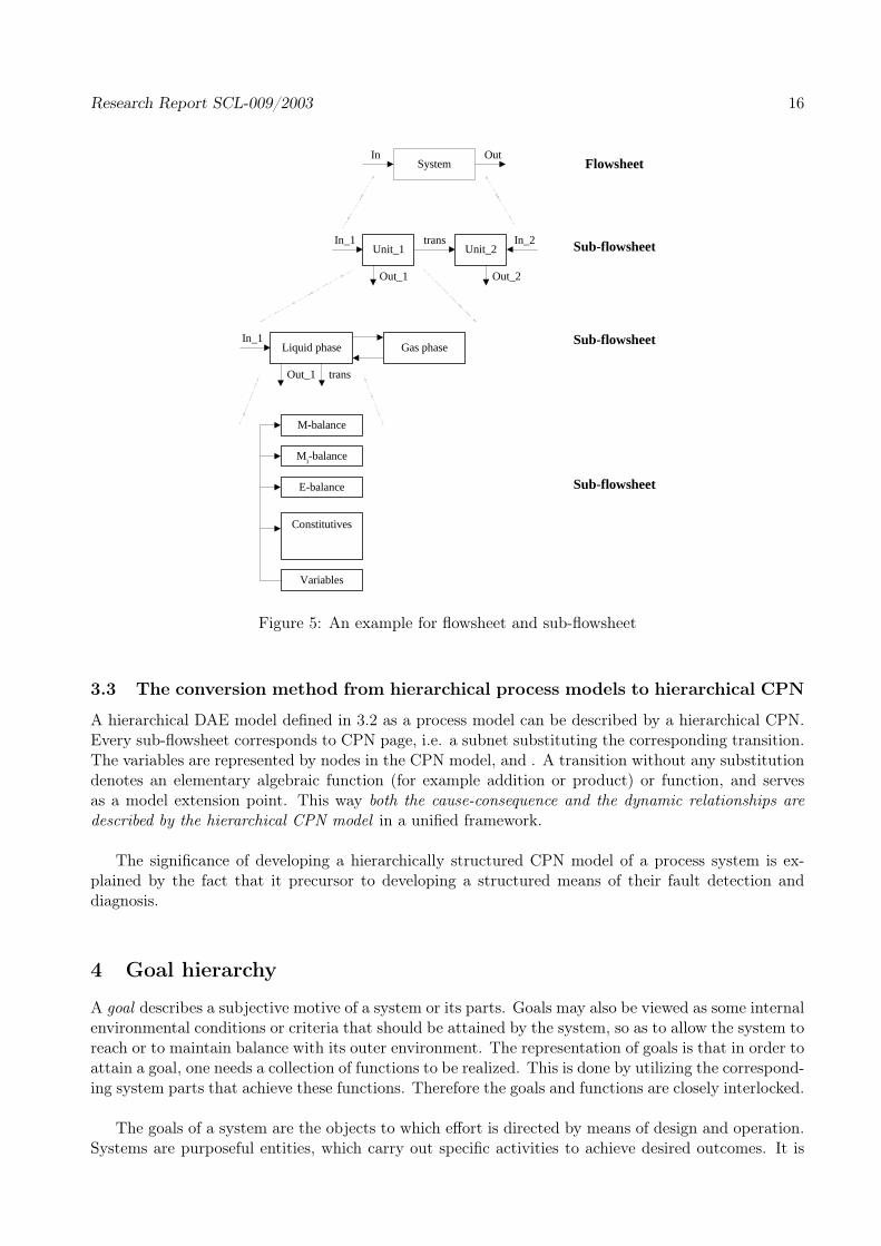
An illustrative example can be seen is Fig. 5. The highest level represents the system with inputand output. In the next level (as sub-flowsheet) represents the more detailed system description, in theexample the system is divided into two units which are connected. Unit_1 consists of two phases (agas and a liquid) described by the 3rd layer. In the next layer the liquid phase is detailed by equations.

The elements of a hierarchical differential algebraic equation (HDAE) process model are then asfollows:

• units which contains some phases on the same hierarchical level, but all of them correspond to asub-flowsheet.

• balance equations connected to a unit or a phase that is on the same hierarchical level, but allof them correspond to a sub-flowsheet.

• variables used in a balance equation and described by a constitutive algebraic equation aredetailed in a sub-flowsheet, i.e. the sub-flowsheet models the corresponding constitutive algebraicequation.

• variables used in an complementary algebraic equation and described by an algebraic equationare also detailed in a sub-flowsheet, i.e. the sub-flowsheet models the corresponding algebraicequation.


System

Liquid phase

M-balance

E-balance

Constitutives

Variables

In

Mi-balance

Out

Unit_1 Unit_2transIn_1 In_2

Out_1 Out_2

In_1

Out_1 trans

Gas phase

Flowsheet

Sub-flowsheet

Sub-flowsheet

Sub-flowsheet

Figure 5: An example for flowsheet and sub-flowsheet

3.3 The conversion method from hierarchical process models to hierarchical CPN

A hierarchical DAE model defined in 3.2 as a process model can be described by a hierarchical CPN.Every sub-flowsheet corresponds to CPN page, i.e. a subnet substituting the corresponding transition.The variables are represented by nodes in the CPN model, and . A transition without any substitutiondenotes an elementary algebraic function (for example addition or product) or function, and servesas a model extension point. This way both the cause-consequence and the dynamic relationships aredescribed by the hierarchical CPN model in a unified framework.

The significance of developing a hierarchically structured CPN model of a process system is ex-plained by the fact that it precursor to developing a structured means of their fault detection anddiagnosis.

4 Goal hierarchy

A goal describes a subjective motive of a system or its parts. Goals may also be viewed as some internalenvironmental conditions or criteria that should be attained by the system, so as to allow the system toreach or to maintain balance with its outer environment. The representation of goals is that in order toattain a goal, one needs a collection of functions to be realized. This is done by utilizing the correspond-ing system parts that achieve these functions. Therefore the goals and functions are closely interlocked.

The goals of a system are the objects to which effort is directed by means of design and operation.Systems are purposeful entities, which carry out specific activities to achieve desired outcomes. It is


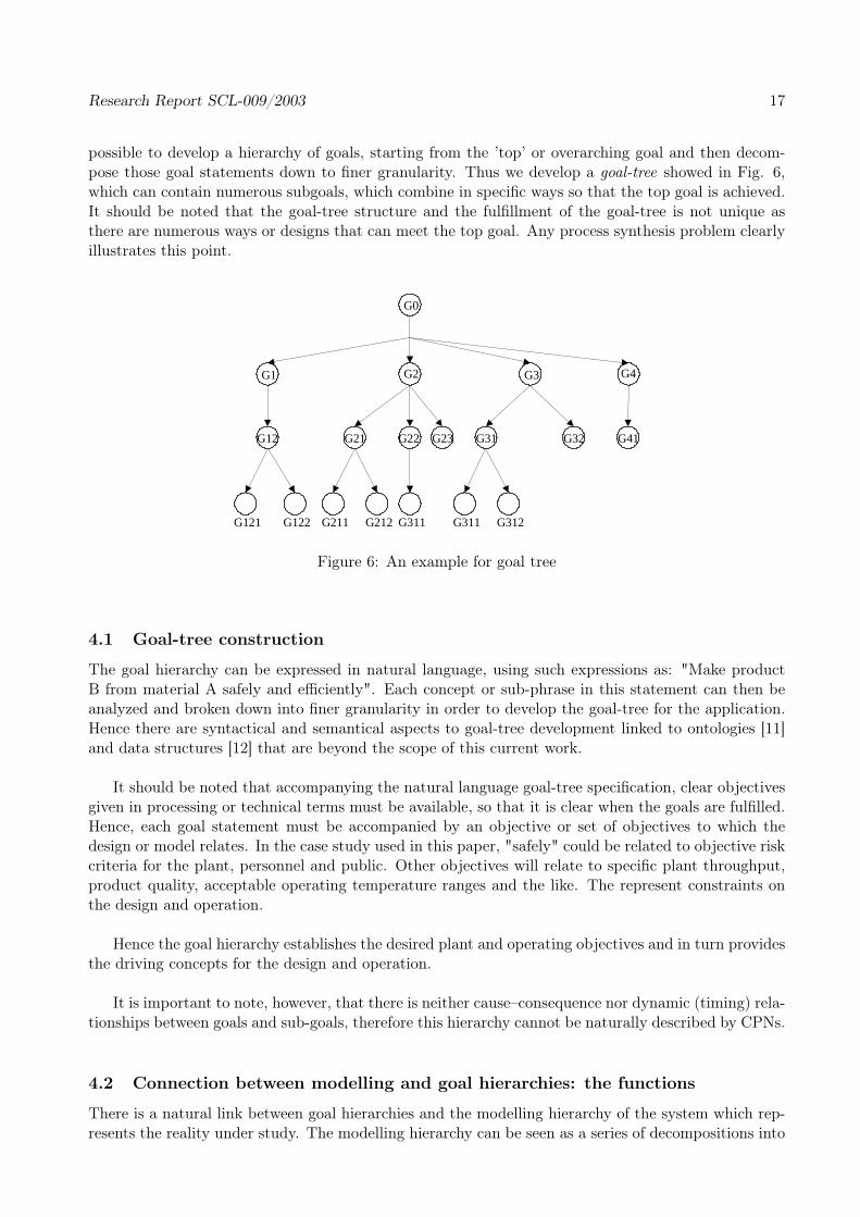
possible to develop a hierarchy of goals, starting from the ’top’ or overarching goal and then decom-pose those goal statements down to finer granularity. Thus we develop a goal-tree showed in Fig. 6,which can contain numerous subgoals, which combine in specific ways so that the top goal is achieved.It should be noted that the goal-tree structure and the fulfillment of the goal-tree is not unique asthere are numerous ways or designs that can meet the top goal. Any process synthesis problem clearlyillustrates this point.

G0

G1 G2 G3

G121

G4

G41G31 G32

G312G311G122

G21 G23

G212G211

G22

G311

G12

Figure 6: An example for goal tree

4.1 Goal-tree construction

The goal hierarchy can be expressed in natural language, using such expressions as: "Make productB from material A safely and efficiently". Each concept or sub-phrase in this statement can then beanalyzed and broken down into finer granularity in order to develop the goal-tree for the application.Hence there are syntactical and semantical aspects to goal-tree development linked to ontologies [11]and data structures [12] that are beyond the scope of this current work.

It should be noted that accompanying the natural language goal-tree specification, clear objectivesgiven in processing or technical terms must be available, so that it is clear when the goals are fulfilled.Hence, each goal statement must be accompanied by an objective or set of objectives to which thedesign or model relates. In the case study used in this paper, "safely" could be related to objective riskcriteria for the plant, personnel and public. Other objectives will relate to specific plant throughput,product quality, acceptable operating temperature ranges and the like. The represent constraints onthe design and operation.

Hence the goal hierarchy establishes the desired plant and operating objectives and in turn providesthe driving concepts for the design and operation.

It is important to note, however, that there is neither cause–consequence nor dynamic (timing) rela-tionships between goals and sub-goals, therefore this hierarchy cannot be naturally described by CPNs.

4.2 Connection between modelling and goal hierarchies: the functions

There is a natural link between goal hierarchies and the modelling hierarchy of the system which rep-resents the reality under study. The modelling hierarchy can be seen as a series of decompositions into


finer levels of granularity: from the plant-wide model down to the equation and variable representation.

Goal nodes (G1, G2, . . .) in the goal tree are addressed by specific functionality in the system com-ponents or their combinations. These physico-chemical components can be ultimately expressed interms of equations and variables at the lowest modelling level. Hence there is a mapping of the modelhierarchy through a function/behaviour hierarchy to the goal hierarchy.

Functions represent the roles of a system should have intended in the achievement of the goals. Anode of a goal tree represents just an achieve goal, but the fulfilling way isn’t described in here. Thesymptom connected to a goal node contains a function/behaviour like the knowledge, as condition of agoal (i.e. how the connected goal is reached). If the condition in a symptom is fulfilled, the connectedgoal is reached, otherwise some deviance is occurring. That is a connecting point for fault detectionand diagnosis.

The hierarchies between model elements and between subgoals give a natural hierarchy betweenthe symptoms.

The function/behaviour hierarchy is based upon the concept of a "function" which is a functionalof the elements in the model hierarchy in an abstract sense. A function serves one or more goalsin the goal hierarchy and thus it is a "connector" between the model elements it depends upon andthe goal(s) it serves. Furthermore, functions may have “symptoms", i.e. deviations from the normalbehavior associated to them, therefore they can be used as abstract “indicators" for fault detectionand diagnosis.

So, the modelling hierarchy at the equation-variable level addresses lower subgoals and the com-posite modelling structures as we proceed up the tree are also logically linked to the upper goals inthe goal-tree.

Furthermore, the fault detection and diagnosis, that can be performed using coloured Petri nets,can be connected to the hierarchical model CPN through connecting "function" nodes.

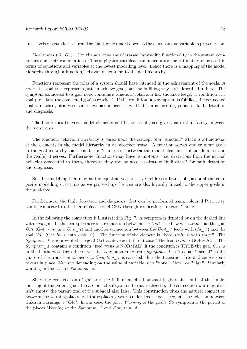
In the following the connection is illustrated in Fig. 7. A symptom is denoted by on the dashed linewith hexagon. In the example there is a connection between the Unit_2 inflow with trans and the goalG31 (Get trans into Unit_2 ) and another connection between the Unit_2 feeds with (In_2 ) and thegoal G32 (Get In_2 into Unit_2 ) . The function of the element is "Feed Unit_2 with trans". TheSymptom_1 is represented the goal G31 achievement, in out case "The feed trans is NORMAL". TheSymptom_1 contains a condition "feed trans is NORMAL" If the condition is TRUE the goal G31 isfulfilled, otherwise the value of variable sign outcoming from Symptom_1 isn’t equal "normal" so theguard of the transition connects to Symptom_1 is satisfied, thus the transition fires and causes sometokens in place Warning depending on the value of variable sign "none", "low" or "high". Similarlyworking in the case of Symptom_2.

Since the construction of goal-tree the fulfillment of all subgoal is gives the truth of the imple-menting of the parent goal. In case one of subgoal isn’t true, realized by the connection warning placeisn’t empty, the parent goal of the subgoal also false. This construction gives the natural connectionbetween the warning places, but these places gives a similar tree as goal-tree, but the relation betweenchildren warnings is "OR". In our case, the place Warning of the goal’s G3 symptom is the parent ofthe places Warning of the Symptom_1 and Symptom_2.


System

Liquid phase

In Out

Unit_1 Unit_2transIn_1 In_2

Out_1 Out_2

In_1

Out_1 trans

Gas phase

G0

G1 G2 G3

G121

G4

G41G31 G32

G312G311G122

G21 G23

G212G211

G22

G311

G12Get transinto Unit_2

Get In_2into Unit_2

Get inputsinto Unit_2

[sign<> nomal]

Warning

sign msg

[sign<> nomal]

Warning

sign msg

Symp-tom_1 Symp-

tom_2

Figure 7: An example for the connection between the modelling and goal hierarchies with symptoms

5 Case study: A tank reactor with cooling jacket

In the following example simple multi-scale process models will be used to demonstrate the integrateddevelopment of the modelling and goal hierarchies for fault prediction-based fault-detection and diag-nosis purposes.

5.1 The description of the tank reactor with cooling jacket

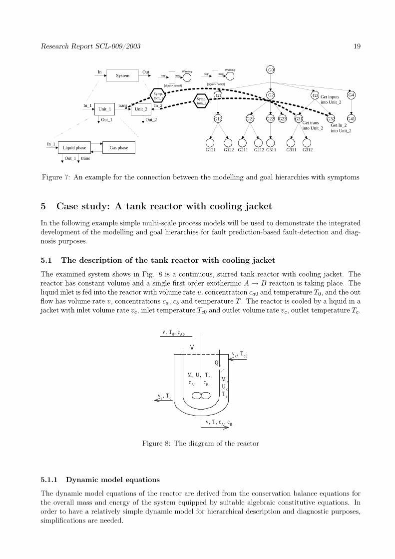
The examined system shows in Fig. 8 is a continuous, stirred tank reactor with cooling jacket. Thereactor has constant volume and a single first order exothermic A → B reaction is taking place. Theliquid inlet is fed into the reactor with volume rate v, concentration ca0 and temperature T0, and the outflow has volume rate v, concentrations ca, cb and temperature T . The reactor is cooled by a liquid in ajacket with inlet volume rate vc, inlet temperature Tc0 and outlet volume rate vc, outlet temperature Tc.

v , T 0 , cA 0

v , T, cA , cB

M, U, T ,c A , cB

v c , T c 0

v c , T c

M cU cT c

Q

Figure 8: The diagram of the reactor

5.1.1 Dynamic model equations

The dynamic model equations of the reactor are derived from the conservation balance equations forthe overall mass and energy of the system equipped by suitable algebraic constitutive equations. Inorder to have a relatively simple dynamic model for hierarchical description and diagnostic purposes,simplifications are needed.


Modelling assumptions

(i) The liquid in the tank reactor and in the cooling jacket is perfectly stirred.

(ii) There is only cooling liquid (water) in the jacket.

(iii) Balances are only set up for liquid phase in the tank reactor (the gas phase is neglected).

(iv) Physico-chemical properties are constant.

(v) The liquid phase in the tank has a constant volume V .

(vi) There are 3 components in the tank: A, B and inert (water).

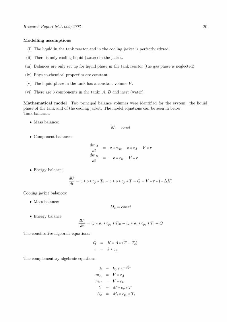
Mathematical model Two principal balance volumes were identified for the system: the liquidphase of the tank and of the cooling jacket. The model equations can be seen in below.Tank balances:

• Mass balance:M = const

• Component balances:

dmA

dt= v ∗ cA0 − v ∗ cA − V ∗ r

dmB

dt= −v ∗ cB + V ∗ r

• Energy balance:

dU

dt= v ∗ ρ ∗ cp ∗ T0 − v ∗ ρ ∗ cp ∗ T − Q + V ∗ r ∗ (−∆H)

Cooling jacket balances:

• Mass balance:Mc = const

• Energy balancedUc

dt= vc ∗ ρc ∗ cpc ∗ Tc0 − vc ∗ ρc ∗ cpc ∗ Tc + Q

The constitutive algebraic equations:

Q = K ∗ A ∗ (T − Tc)

r = k ∗ cA

The complementary algebraic equations:

k = k0 ∗ e−E

R∗T

mA = V ∗ cA

mB = V ∗ cB

U = M ∗ cp ∗ T

Uc = Mc ∗ cpc ∗ Tc


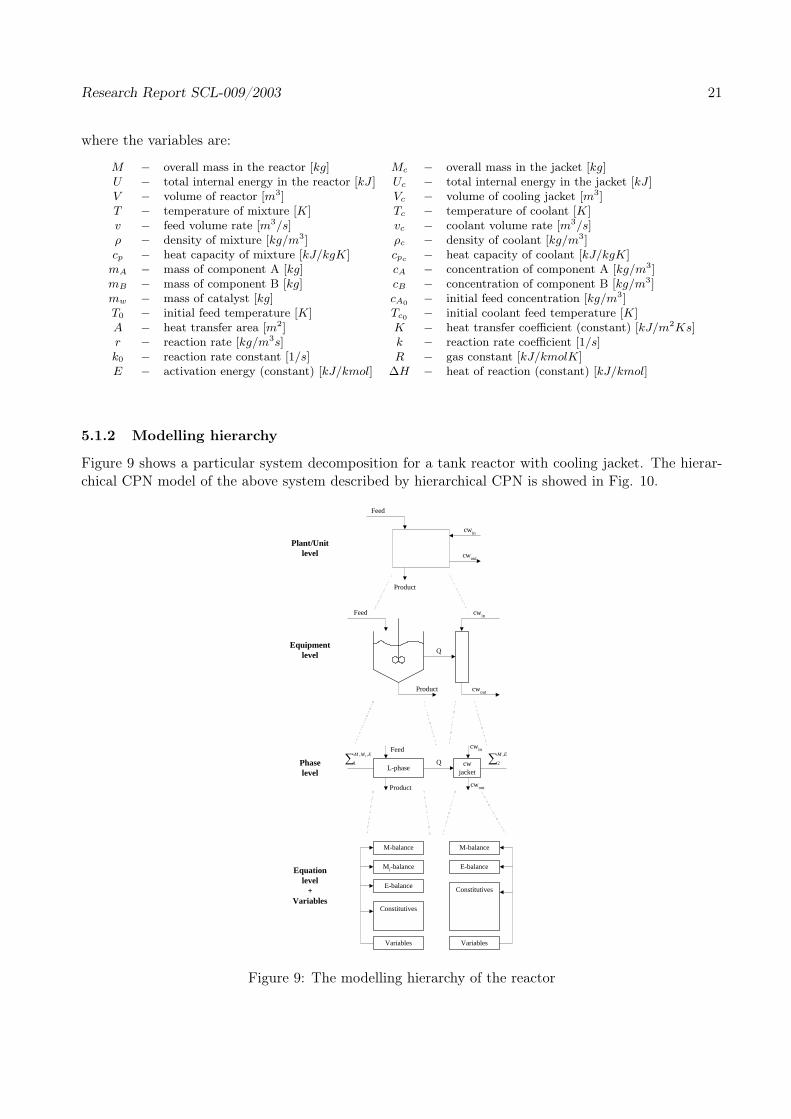
where the variables are:

M − overall mass in the reactor [kg] Mc − overall mass in the jacket [kg]U − total internal energy in the reactor [kJ ] Uc − total internal energy in the jacket [kJ ]V − volume of reactor [m3] Vc − volume of cooling jacket [m3]T − temperature of mixture [K] Tc − temperature of coolant [K]v − feed volume rate [m3/s] vc − coolant volume rate [m3/s]ρ − density of mixture [kg/m3] ρc − density of coolant [kg/m3]cp − heat capacity of mixture [kJ/kgK] cpc

− heat capacity of coolant [kJ/kgK]mA − mass of component A [kg] cA − concentration of component A [kg/m3]mB − mass of component B [kg] cB − concentration of component B [kg/m3]mw − mass of catalyst [kg] cA0

− initial feed concentration [kg/m3]T0 − initial feed temperature [K] Tc0 − initial coolant feed temperature [K]A − heat transfer area [m2] K − heat transfer coefficient (constant) [kJ/m2Ks]r − reaction rate [kg/m3s] k − reaction rate coefficient [1/s]k0 − reaction rate constant [1/s] R − gas constant [kJ/kmolK]E − activation energy (constant) [kJ/kmol] ∆H − heat of reaction (constant) [kJ/kmol]

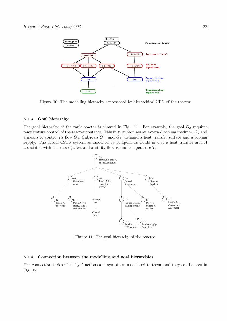
5.1.2 Modelling hierarchy

Figure 9 shows a particular system decomposition for a tank reactor with cooling jacket. The hierar-chical CPN model of the above system described by hierarchical CPN is showed in Fig. 10.

L-phasecw

jacket

M-balance

E-balance

Constitutives

Variables

E-balance

Constitutives

Variables

Feed

Product

cwin

cwout

Q

Feed

Product

cwin

cwout

cwin

cwoutProduct

Feed

Q

Equipmentlevel

Plant/Unitlevel

Phaselevel

Equationlevel

+Variables

∑ EMM i ,,

1 ∑ EM ,

2

Mi-balance

M-balance

Figure 9: The modelling hierarchy of the reactor


Figure 10: The modelling hierarchy represented by hierarchical CPN of the reactor

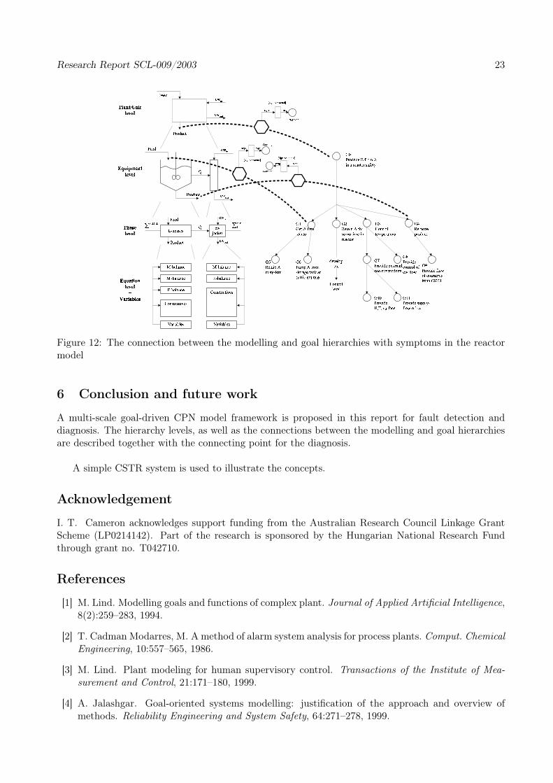
5.1.3 Goal hierarchy

The goal hierarchy of the tank reactor is showed in Fig. 11. For example, the goal G3 requirestemperature control of the reactor contents. This in turn requires an external cooling medium, G7 anda means to control its flow G8. Subgoals G10 and G11 demand a heat transfer surface and a coolingsupply. The actual CSTR system as modelled by components would involve a heat transfer area Aassociated with the vessel-jacket and a utility flow vc and temperature Tc.

G0Produce B from Ain a reactor safety

G1Get A intoreactor

G2Retain A forsome time inreactor

G3Controltemperature

G5Retain Ain system

G6Pump A fromstorage tank atsufficient rate

G4Removeproduct

G9Provide flowof countentsfrom CSTR

G7Provide externalcooling medium

G8Providecontrol ofcw flow

G11Provide supply/flow of cw

G10ProvideH.T. surface

developetc

Controllevel

Figure 11: The goal hierarchy of the reactor

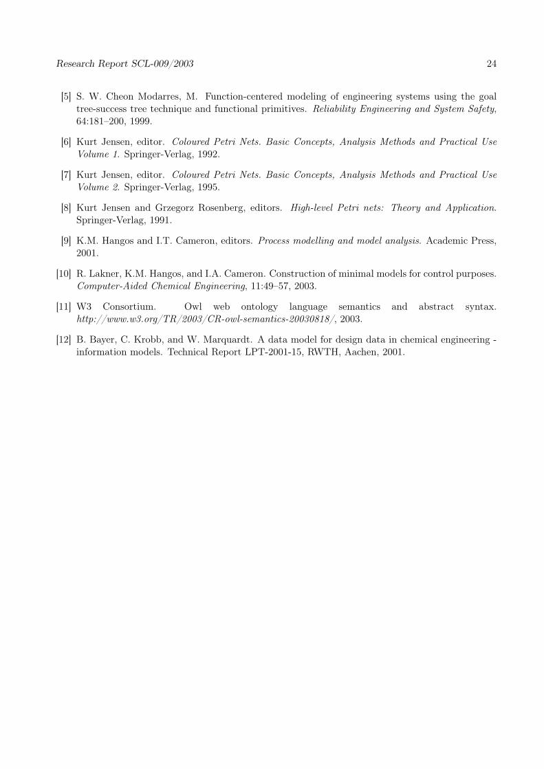
5.1.4 Connection between the modelling and goal hierarchies

The connection is described by functions and symptoms associated to them, and they can be seen inFig. 12.


Figure 12: The connection between the modelling and goal hierarchies with symptoms in the reactormodel

6 Conclusion and future work

A multi-scale goal-driven CPN model framework is proposed in this report for fault detection anddiagnosis. The hierarchy levels, as well as the connections between the modelling and goal hierarchiesare described together with the connecting point for the diagnosis.

A simple CSTR system is used to illustrate the concepts.

Acknowledgement

I. T. Cameron acknowledges support funding from the Australian Research Council Linkage GrantScheme (LP0214142). Part of the research is sponsored by the Hungarian National Research Fundthrough grant no. T042710.

References

[1] M. Lind. Modelling goals and functions of complex plant. Journal of Applied Artificial Intelligence,8(2):259–283, 1994.

[2] T. Cadman Modarres, M. A method of alarm system analysis for process plants. Comput. ChemicalEngineering, 10:557–565, 1986.

[3] M. Lind. Plant modeling for human supervisory control. Transactions of the Institute of Mea-surement and Control, 21:171–180, 1999.

[4] A. Jalashgar. Goal-oriented systems modelling: justification of the approach and overview ofmethods. Reliability Engineering and System Safety, 64:271–278, 1999.


[5] S. W. Cheon Modarres, M. Function-centered modeling of engineering systems using the goaltree-success tree technique and functional primitives. Reliability Engineering and System Safety,64:181–200, 1999.

[6] Kurt Jensen, editor. Coloured Petri Nets. Basic Concepts, Analysis Methods and Practical UseVolume 1. Springer-Verlag, 1992.

[7] Kurt Jensen, editor. Coloured Petri Nets. Basic Concepts, Analysis Methods and Practical UseVolume 2. Springer-Verlag, 1995.

[8] Kurt Jensen and Grzegorz Rosenberg, editors. High-level Petri nets: Theory and Application.Springer-Verlag, 1991.

[9] K.M. Hangos and I.T. Cameron, editors. Process modelling and model analysis. Academic Press,2001.

[10] R. Lakner, K.M. Hangos, and I.A. Cameron. Construction of minimal models for control purposes.Computer-Aided Chemical Engineering, 11:49–57, 2003.

[11] W3 Consortium. Owl web ontology language semantics and abstract syntax.http://www.w3.org/TR/2003/CR-owl-semantics-20030818/, 2003.

[12] B. Bayer, C. Krobb, and W. Marquardt. A data model for design data in chemical engineering -information models. Technical Report LPT-2001-15, RWTH, Aachen, 2001.

Documents

Hierarchical CPN model-based diagnosis using HAZOP …daedalus.scl.sztaki.hu/pdf/research reports/NemethE.pdf · Hierarchical CPN model-based diagnosis using ... a description of