Hierarchical Insurance Claims Modeling�

Edward W. FreesUniversity of Wisconsin

Emiliano A. ValdezUniversity of New South Wales

02-February-2007y

AbstractThis work describes statistical modeling of detailed, micro-level automobile in-

surance records. We consider 1993-2001 data from a major insurance company inSingapore. By detailed micro-level records, we refer to experience at the individual ve-hicle level, including vehicle and driver characteristics, insurance coverage and claimsexperience, by year. The claims experience consists of detailed information on thetype of insurance claim, such as whether the claim is due to injury to a third party,property damage to a third party or claims for damage to the insured, as well as thecorresponding claim amount.

We propose a hierarchical model for three components, corresponding to the fre-quency, type and severity of claims. The �rst is a negative binomial regression modelfor assessing claim frequency. The driver�s gender, age, and no claims discount as wellas vehicle age and type turn out to be important variables for predicting the event of aclaim. The second is a multinomial logit model to predict the type of insurance claim,whether it is third party injury, third party property damage, insured�s own damageor some combination. Year, vehicle age and vehicle type turn out to be importantpredictors for this component.

Our third model is for the severity component. Here, we use a generalized betaof the second kind long-tailed distribution for claim amounts and also incorporatepredictor variables. Year, vehicle age and a person�s age turn out to be importantpredictors for this component. Not surprisingly, we show that there is a signi�cantdependence among the di¤erent claim types; we use a t-copula to account for thisdependence.

The three component model provides justi�cation for assessing the importanceof a rating variable. When taken together, the integrated model allows an actuary topredict automobile claims more e¢ ciently than traditional methods. Using simulation,we demonstrate this by developing predictive distributions and calculating premiumsunder alternative reinsurance coverages.

�Keywords: Long-tail regression and copulas.yThe authors acknowledge the research assistance of Mitchell Wills, Shi Peng and Katrien

Antonio. The �rst author thanks the National Science Foundation (Grant Number SES-0436274) and the Assurant Health Insurance Professorship for funding to support thisresearch. The second author thanks the Australian Research Council through the DiscoveryGrant DP0345036 and the UNSW Actuarial Foundation of the Institute of Actuaries ofAustralia for �nancial support. Please do not quote without the authors�permission.

1

1 Introduction

A primary attribute of the actuary has been the ability to successfully apply statis-tical techniques in the analysis and interpretation of data. In this paper, we analyzea highly complex data structure and demonstrate the use of modern statistical tech-niques in solving actuarial problems. Speci�cally, we focus on a portfolio of motor(or automobile) insurance policies and, in analyzing the historical data drawn fromthis portfolio, we are able to re-visit some of the classical problems faced by actuar-ies dealing with insurance data. This paper explores statistical models that can beconstructed when detailed, micro-level records of automobile insurance policies areavailable.To an actuarial audience, the paper provides a fresh look into the process of

modeling and estimation of insurance data. For a statistical audience, we wish toemphasize:

� the highly complex data structure, making the statistical analysis and proce-dures interesting. Despite this complexity, the automobile insurance problem iscommon and many readers will be able to relate to the data.

� the long-tail nature of the distribution of insurance claims. This, and the multi-variate nature of di¤erent claim types, is of broad interest. Using the additionalinformation provided by the frequency and type of claims, the actuary will beable to provide more accurate estimates of the claims distribution.

� the interpretation of the models and their results. We introduce a hierarchical,three-component model structure to help interpret our complex data.

In analyzing the data, we focus on two concerns of the actuary. First, there isa consensus, at least for motor insurance, of the importance of identifying key ex-planatory variables for rating purposes, see for example, LeMaire (1985) or the guideavailable from the General Insurance Association (G.I.A.) of Singapore1. Insurersoften adopt a so-called �risk factor rating system�in establishing premiums for mo-tor insurance so that identifying these important risk factors is a crucial process indeveloping insurance rates. To illustrate, these risk factors include driver (e.g. age,gender) and vehicle (e.g. make/brand/model of car, cubic capacity) characteristics.Second is one of the most important aspects of the actuary�s job: to be able to

predict claims as accurately as possible. Actuaries require accurate predictions forpricing, for estimating future company liabilities, and for understanding the implica-tions of these claims to the solvency of the company. For example, in pricing the ac-tuary may attempt to segregate the �good drivers�from the �bad drivers�and assessthe proper increment in the insurance premium for those considered �bad drivers.�

1See the organization�s website at: http://www.gia.org.sg.

2

This process is important to ensure equity in the premium structure available to theconsumers.In this paper, we consider policy exposure and claims experience data derived from

vehicle insurance portfolios from a major general insurance company in Singapore.Our data are from the General Insurance Association of Singapore, an organizationconsisting of most of the general insurers in Singapore. The observations are fromeach policyholder over a period of nine years: January 1993 until December 2001.Thus, our data comes from �nancial records of automobile insurance policies. Inmany countries, owners of automobiles are not free to drive their vehicles withoutsome form of insurance coverage. Singapore is no exception; it requires drivers tohave minimum coverage for personal injury to third parties.We examined three databases: the policy, claims and payment �les. The policy �le

consists of all policyholders with vehicle insurance coverage purchased from a generalinsurer during the observation period. Each vehicle is identi�ed with a unique code.This �le provides characteristics of the policyholder and the vehicle insured, such asage and gender and type and age of vehicle insured. The claims �le provides a recordof each accident claim that has been �led with the insurer during the observationperiod and is linked to the policyholder �le. The payment �le consists of informationon each payment that has been made during the observation period and is linked tothe claims �le. It is common to see that a claim will have multiple payments made.In predicting or estimating claims distributions, at least for motor insurance, we

often associate the cost of claims with two components: the event of an accident andthe amount of claim, if an accident occurs. Actuaries term these the claims frequencyand severity components, respectively. This is the traditional way of decomposingthis so-called �two-part�data, where one can think of a zero as arising from a vehiclewithout a claim. This decomposition easily allows us to incorporate having multipleclaims per vehicle. Moreover, records from our databases show that when a claimpayment is made, we can also identify the type of claim. For our data, there are threetypes: (1) claims for injury to a party other than the insured, (2) claims for damagesto the insured including injury, property damage, �re and theft, and (3) claims forproperty damage to a party other than the insured. Identifying the type of claim istraditionally done through a �multidecrement�model such as one might encounter ina competing risks framework in biostatistics. See, for example, Bowers et al. (1997),for an actuarial introduction to two-part data (Chapter 2) and multidecrement models(Chapter 10).Thus, instead of a traditional univariate claim analysis, we potentially observe a

trivariate claim amount, one claim for each type. For each accident, it is possible tohave more than a single type of claim incurred; for example, an automobile accidentcan result in damages to a driver�s own property as well as damages to a third partywho might be involved in the accident. Modelling therefore the joint distribution ofthe simultaneous occurrence of these claim types, when an accident occurs, providesthe unique feature in this paper. From a multivariate analysis standpoint, this is a

3

nonstandard problem in that we rarely observe all three claim types simultaneously(see Section 3.3 for the distribution of claim types). Not surprisingly, it turns outthat claim amounts among types are related. To further complicate matters, it turnsout that one type of claim is censored (see Section 2.1). We use copula functionsto specify the joint multivariate distribution of the claims arising from these variousclaims types. See Frees and Valdez (1998) and Nelsen (1999) for introductions tocopula modeling.To provide focus, we restrict our considerations to �non-�eet�policies; these com-

prise about 90% of the policies for this company. These are policies issued to cus-tomers whose insurance covers a single vehicle. In contrast, �eet policies are issued tocompanies that insured several vehicles, for example, coverage provided to a taxicabcompany, where several taxicabs are insured. See Angers et al. (2006) and Desjardinset al. (2001) for discussions of �eet policies. The unit of observation in our analysisis therefore a registered vehicle insured, broken down according to their exposure ineach calendar year 1993 to 2001. In order to investigate the full multivariate natureof claims, we further restrict our consideration to policies that o¤er comprehensivecoverage, not merely for only third party injury or property damage.In constructing the models for our portfolio of policies, we therefore focus on

the development of the claims distribution according to three di¤erent components:(1) the claims frequency, (2) the conditional claim type, and (3) the conditionalseverity. The claims frequency provides the likelihood that an insured registeredvehicle will have an accident and will make a claim in a given calendar year. Giventhat a claim is to be made when an accident occurs, the conditional claim typemodel describes the probability that it will be one of the three claim types, or anypossible combination of them. The conditional severity component describes the claimamount structure according to the combination of claim types paid. In this paper,we provide appropriate statistical models for each component, emphasizing that theunique feature of this decomposition is the joint multivariate modeling of the claimamounts arising from the various claim types. Because of the short term nature of theinsurance coverages investigated here, we summarize the many payments per claiminto a single claim amount. See Antonio et al. (2006) for a recent description of theclaims �run-o¤�problem.The organization of the rest of the paper is as follows. First, in Section 2, we

introduce the observable data, summarize its important characteristics and providedetails of the statistical models chosen for each of the three components of frequency,conditional claim type and conditional severity. In Section 3, we proceed with �ttingthe statistical model to the data and interpreting the results. The likelihood functionconstruction for the estimation of the conditional severity component is detailed inthe Appendix. In Section 4, we describe how one can use the modeling constructionand results. We provide concluding remarks in Section 5.

4

2 Modeling

2.1 Data Structure

As explained in the introduction, the data available are disaggregated by risk class i,denoting insured vehicle, and over time t, denoting calendar year. For each observa-tional unit fitg then, the potentially observable responses consist of:

� Nit - the number of claims within a year;

� Mit;j - the type of claim, available for each claim, j = 1; :::; Nit; and

� Cit;jk - the claim amount, available for each claim, j = 1; :::; Nit, and for eachtype of claim k = 1; 2; 3.

When a claim is made, it is possible to have one or a combination of three typesof claims. To reiterate, we consider: (1) claims for injury to a party other than theinsured, (2) claims for damages to the insured, including injury, property damage,�re and theft, and (3) claims for property damage to a party other than the insured.Occasionally, we shall simply refer to them as �injury,� �own damage� and �thirdparty property.�It is not uncommon to have more than one type of claim incurredwith each accident.For the two third party types, loss amounts are available. However, for damages

to the insured (�own damages�), only a claim amount is available. Here, we followstandard actuarial terminology and de�ne the claim amount, Cit;2k, to be equal tothe excess of a loss over a known deductible, dit (and equal to zero if the loss is lessthan the deductible). For notation purposes, we will sometimes use C�it;2k to denotethe loss amount; this quantity is not known when it falls below the deductible. Thus,it is possible to observe a zero claim associated with an �own damages�claim. Forour analysis, we assume that the deductibles apply on a per accident basis.We also have the exposure eit, measured in (a fraction of) years, which provides

the length of time throughout the calendar year for which the vehicle had insurancecoverage. The various vehicle and policyholder characteristics are described by thevector xit and will serve as explanatory variables in our analysis. For notationalpurposes, let Mit denote the vector of claim types for an observational unit andsimilarly for Cit. In summary, the observable data available consist of

fdit; eit; Nit;Mit;Cit;xit; t = 1; : : : ; Ti; i = 1; : : : ; ng:

There are n = 96; 014 subjects for which each subject is observed Ti times. Inprinciple, the maximum value of Ti is 9 years because our data consists of policiesfrom 1993 up until 2001. Even though a policy issued in 2001 may well extendcoverage into 2002, we ignore the exposure and claims behavior beyond 2001. Themotivation is to follow standard accounting periods upon which actuarial reports are

5

based. However, our data set is from an insurance company where there is substantialturnover of policies. For the full data set, there are 199,352 observations arisingfrom 96,014 subjects, for an average of only 2.08 observations per subject. Whenexamining the weights eit, there is on average only 1.29 years of exposure per subject.Thus, although we model the longitudinal behavior of subjects, for this data set therelationship among components turns out to be more relevant.

2.2 Decomposing the Joint Distribution into Components

Suppressing the fitg subscripts, we decompose the joint distribution of the dependentvariables as:

f (N;M;C) = f (N) � f (MjN) � f (CjN;M)joint = frequency � conditional claim type � conditional severity,

where f (N;M;C) denotes the joint distribution of (N;M;C). This joint distributionequals the product of the three components:

1. claims frequency: f (N) denotes the probability of having N claims;

2. conditional claim type: f (MjN) denotes the probability of having a claim typeof M, given N ; and

3. conditional severity: f (CjN;M) denotes the conditional density of the claimvector C given N andM.

It is customary in the actuarial literature to condition on the frequency componentwhen analyzing the joint frequency and severity distributions. See, for example,Klugman, Panjer and Willmot (2004). As described in Section 2.2.2, we incorporatean additional claims type layer. An alternative approach was taken by Pinquet (1998).Pinquet was interested in two lines of business, claims at fault and not at fault withrespect to a third party. For each line, Pinquet hypothesized a frequency and severitycomponent that were allowed to be correlated to one another. In particular, the claimsfrequency distribution was assumed to be bivariate Poisson. In contrast, our approachis to have a univariate claims number process and then decompose each claim via claimtype. As will be seen in Section 2.2.3, we also allow for dependent claim amountsarising from the di¤erent claim types using the copula approach. Under this approach,a wide range of possible dependence structure can be �exibly speci�ed.We now discuss each of the three components in the following subsections.

2.2.1 Frequency Component

The frequency component, f (N), has been well analyzed in the actuarial literatureand we will use these developments. The modern approach of �tting a claims num-ber distribution to longitudinal data can be attributed to the work of Dionne and

6

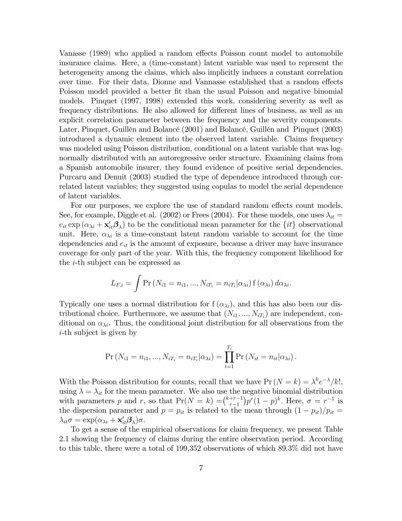
Vanasse (1989) who applied a random e¤ects Poisson count model to automobileinsurance claims. Here, a (time-constant) latent variable was used to represent theheterogeneity among the claims, which also implicitly induces a constant correlationover time. For their data, Dionne and Vannasse established that a random e¤ectsPoisson model provided a better �t than the usual Poisson and negative binomialmodels. Pinquet (1997, 1998) extended this work, considering severity as well asfrequency distributions. He also allowed for di¤erent lines of business, as well as anexplicit correlation parameter between the frequency and the severity components.Later, Pinquet, Guillén and Bolancé (2001) and Bolancé, Guillén and Pinquet (2003)introduced a dynamic element into the observed latent variable. Claims frequencywas modeled using Poisson distribution, conditional on a latent variable that was log-normally distributed with an autoregressive order structure. Examining claims froma Spanish automobile insurer, they found evidence of positive serial dependencies.Purcaru and Denuit (2003) studied the type of dependence introduced through cor-related latent variables; they suggested using copulas to model the serial dependenceof latent variables.For our purposes, we explore the use of standard random e¤ects count models.

See, for example, Diggle et al. (2002) or Frees (2004). For these models, one uses �it =eit exp (��i + x

0it��) to be the conditional mean parameter for the fitg observational

unit. Here, ��i is a time-constant latent random variable to account for the timedependencies and eit is the amount of exposure, because a driver may have insurancecoverage for only part of the year. With this, the frequency component likelihood forthe i-th subject can be expressed as

LF;i =

ZPr (Ni1 = ni1; :::; NiTi = niTij��i) f (��i) d��i:

Typically one uses a normal distribution for f (��i), and this has also been our dis-tributional choice. Furthermore, we assume that (Ni1; :::; NiTi) are independent, con-ditional on ��i. Thus, the conditional joint distribution for all observations from thei-th subject is given by

Pr (Ni1 = ni1; :::; NiTi = niTij��i) =TiYt=1

Pr (Nit = nitj��i) :

With the Poisson distribution for counts, recall that we have Pr (N = k) = �ke��=k!,using � = �it for the mean parameter. We also use the negative binomial distributionwith parameters p and r, so that Pr(N = k) =

�k+r�1r�1

�pr(1 � p)k: Here, � = r�1 is

the dispersion parameter and p = pit is related to the mean through (1 � pit)=pit =�it� = exp(��i + x

0it��)�.

To get a sense of the empirical observations for claim frequency, we present Table2.1 showing the frequency of claims during the entire observation period. Accordingto this table, there were a total of 199,352 observations of which 89.3% did not have

7

any claims. There are a total of 23,522 (=19,224�1 + 1,859�2 + 177�3 + 11�4 +1�5) claims.

Table 2.1. Frequency of ClaimsCount 0 1 2 3 4 5 TotalNumber 178,080 19,224 1,859 177 11 1 199,352Percentage 89.3 9.6 0.9 0.1 0.0 0.0 100.0

2.2.2 Claims Type Component

In Section 2.1, we described the three types of claims which may occur in any com-bination for a given accident: �third party injury,��own damage�and �third partyproperty.�Conditional on having observed at least one type of claim, the randomvariable M describes the combination observed. Table 2.2 provides the distributionof M . For example, we see that third party injury (C1) is the least prevalent. More-over, Table 2.2 shows that all combinations of claims occurred in our data.

Table 2.2. Distribution of Claims, by Claim Type ObservedValue of M 1 2 3 4 5 6 7 TotalClaim Type (C 1) (C 2) (C 3) (C 1 ,C 2) (C 1 ,C 3) (C 2 ,C 3) (C 1 ,C 2 ,C 3)Number 102 17,216 2,899 68 18 3,176 43 23,522Percentage 0.4 73.2 12.3 0.3 0.1 13.5 0.2 100.0

To incorporate explanatory variables, we model the claim type as a multinomiallogit of the form

Pr (M = m) =exp (Vm)P7s=1 exp (Vs)

; (1)

where Vitj;m = x0it�M;m. This is known as a �selection�or �participation�equationin econometrics; see, for example, Jones (2000). Note that for our application, thecovariates do not depend on the accident number j nor on the claim type m althoughwe allow parameters (�M;m) to depend on m.

2.2.3 Severity Component

Table 2.3 provides a �rst look at the severity component of our data. For each typeof claim, we see that the standard deviation exceeds the mean. For nonnegativedata, this suggests using distributions with fatter tails than the normal. Third partyinjury claims, although the least frequent, have the strongest potential for large con-sequences. There are 2,529 (=20,503-17,974) claims for damages to the insured (�owndamages�) that are censored, indicating that a formal mechanism for handling thecensoring is important.

8

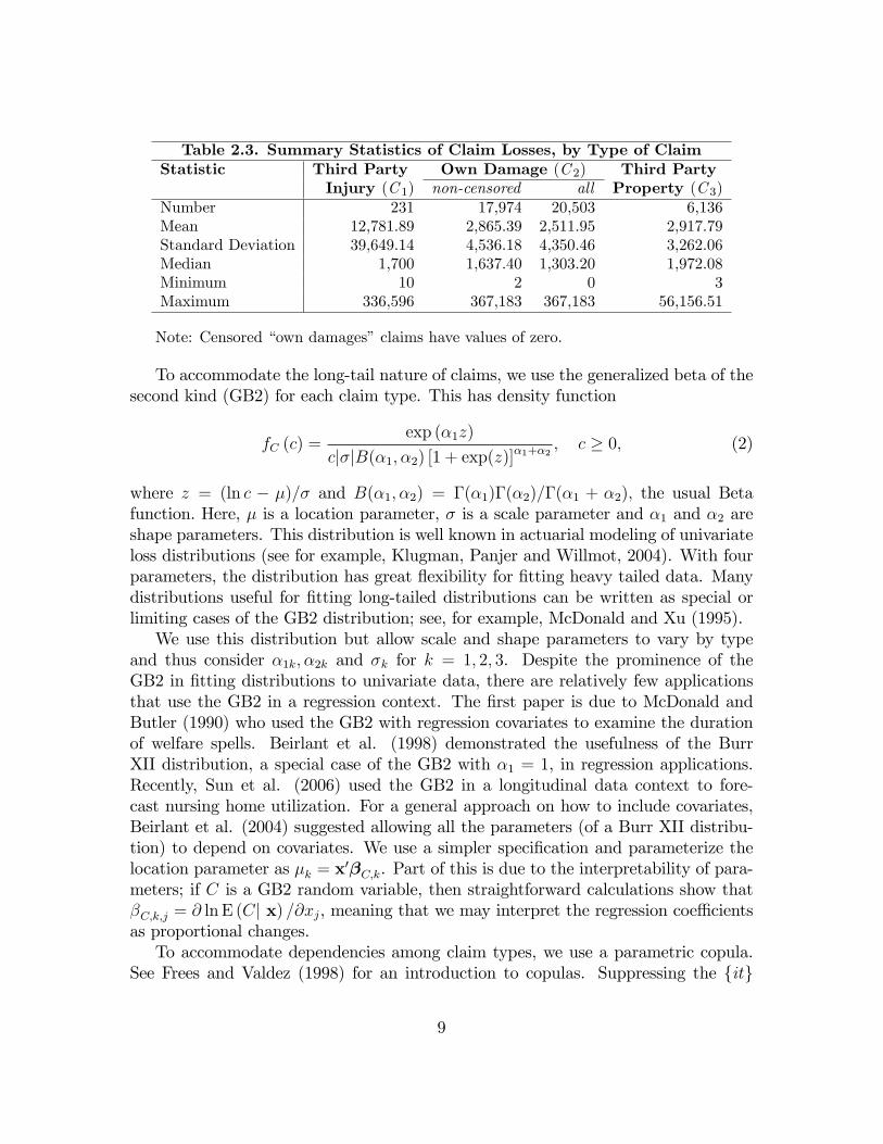
Table 2.3. Summary Statistics of Claim Losses, by Type of ClaimStatistic Third Party Own Damage (C 2) Third Party

Injury (C 1) non-censored all Property (C 3)Number 231 17,974 20,503 6,136Mean 12,781.89 2,865.39 2,511.95 2,917.79Standard Deviation 39,649.14 4,536.18 4,350.46 3,262.06Median 1,700 1,637.40 1,303.20 1,972.08Minimum 10 2 0 3Maximum 336,596 367,183 367,183 56,156.51

Note: Censored �own damages�claims have values of zero.

To accommodate the long-tail nature of claims, we use the generalized beta of thesecond kind (GB2) for each claim type. This has density function

fC (c) =exp (�1z)

cj�jB(�1; �2) [1 + exp(z)]�1+�2; c � 0; (2)

where z = (ln c � �)=� and B(�1; �2) = �(�1)�(�2)=�(�1 + �2); the usual Betafunction. Here, � is a location parameter, � is a scale parameter and �1 and �2 areshape parameters. This distribution is well known in actuarial modeling of univariateloss distributions (see for example, Klugman, Panjer and Willmot, 2004). With fourparameters, the distribution has great �exibility for �tting heavy tailed data. Manydistributions useful for �tting long-tailed distributions can be written as special orlimiting cases of the GB2 distribution; see, for example, McDonald and Xu (1995).We use this distribution but allow scale and shape parameters to vary by type

and thus consider �1k; �2k and �k for k = 1; 2; 3. Despite the prominence of theGB2 in �tting distributions to univariate data, there are relatively few applicationsthat use the GB2 in a regression context. The �rst paper is due to McDonald andButler (1990) who used the GB2 with regression covariates to examine the durationof welfare spells. Beirlant et al. (1998) demonstrated the usefulness of the BurrXII distribution, a special case of the GB2 with �1 = 1, in regression applications.Recently, Sun et al. (2006) used the GB2 in a longitudinal data context to fore-cast nursing home utilization. For a general approach on how to include covariates,Beirlant et al. (2004) suggested allowing all the parameters (of a Burr XII distribu-tion) to depend on covariates. We use a simpler speci�cation and parameterize thelocation parameter as �k = x

0�C;k. Part of this is due to the interpretability of para-meters; if C is a GB2 random variable, then straightforward calculations show that�C;k;j = @ ln E (Cj x) =@xj, meaning that we may interpret the regression coe¢ cientsas proportional changes.To accommodate dependencies among claim types, we use a parametric copula.

See Frees and Valdez (1998) for an introduction to copulas. Suppressing the {it}

9

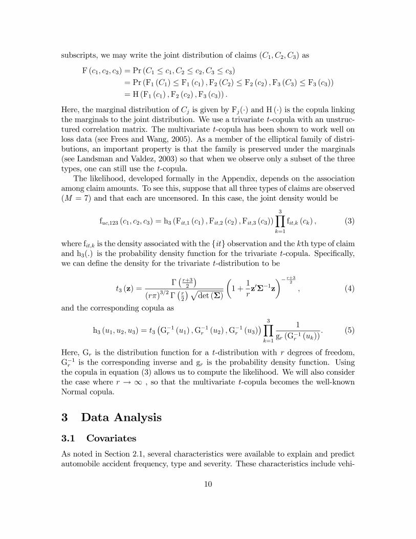
subscripts, we may write the joint distribution of claims (C1; C2; C3) as

F (c1; c2; c3) = Pr (C1 � c1; C2 � c2; C3 � c3)= Pr (F1 (C1) � F1 (c1) ;F2 (C2) � F2 (c2) ;F3 (C3) � F3 (c3))= H (F1 (c1) ;F2 (c2) ;F3 (c3)) :

Here, the marginal distribution of Cj is given by Fj(�) and H(�) is the copula linkingthe marginals to the joint distribution. We use a trivariate t-copula with an unstruc-tured correlation matrix. The multivariate t-copula has been shown to work well onloss data (see Frees and Wang, 2005). As a member of the elliptical family of distri-butions, an important property is that the family is preserved under the marginals(see Landsman and Valdez, 2003) so that when we observe only a subset of the threetypes, one can still use the t-copula.The likelihood, developed formally in the Appendix, depends on the association

among claim amounts. To see this, suppose that all three types of claims are observed(M = 7) and that each are uncensored. In this case, the joint density would be

fuc;123 (c1; c2; c3) = h3 (Fit;1 (c1) ;Fit;2 (c2) ;Fit;3 (c3))

3Yk=1

fit;k (ck) ; (3)

where fit;k is the density associated with the {it} observation and the kth type of claimand h3(.) is the probability density function for the trivariate t-copula. Speci�cally,we can de�ne the density for the trivariate t-distribution to be

t3 (z) =��r+32

�(r�)3=2 �

�r2

�pdet (�)

�1 +

1

rz0��1z

�� r+32

; (4)

and the corresponding copula as

h3 (u1; u2; u3) = t3�G�1r (u1) ;G

�1r (u2) ;G

�1r (u3)

� 3Yk=1

1

gr (G�1r (uk)): (5)

Here, Gr is the distribution function for a t-distribution with r degrees of freedom,G�1r is the corresponding inverse and gr is the probability density function. Usingthe copula in equation (3) allows us to compute the likelihood. We will also considerthe case where r ! 1 , so that the multivariate t-copula becomes the well-knownNormal copula.

3 Data Analysis

3.1 Covariates

As noted in Section 2.1, several characteristics were available to explain and predictautomobile accident frequency, type and severity. These characteristics include vehi-

10

cle characteristics, such as type and age, as well as person level characteristics, such asage, gender and prior driving experience. Table 3.1 summarizes these characteristics.

Table 3.1 Description of CovariatesCovariate DescriptionYear The calendar year, from 1993-2001, inclusive.Vehicle Type The type of vehicle being insured, either automobile (A) or

other (O).Vehicle Age The age of the vehicle, in years, grouped into seven categories.Gender The policyholder�s gender, either male or femaleAge The age of the policyholder, in years, grouped into seven

categories.NCD No Claims Discount. This is based on the previous accident

record of the policyholder.The higher the discount, the better is the prior accidentrecord.

The Section 2 description uses a generic vector x to indicate the availability ofcovariates that are common to the three outcome variables. In our investigation, wefound that the usefulness of covariates depended on the type of outcome and used aparsimonious selection of covariates for each type. The following subsections describehow the covariates can be used to �t our frequency, type and severity models. Forcongruence with Section 2, the data summaries refer to the full data set that compriseyears 1993-2001, inclusive. However, when �tting models, we only used 1993-2000, in-clusive. We reserved observations in year 2001 for out-of-sample validation, discussedin Section 4.

3.2 Fitting the Frequency Component Model

We begin by displaying summary statistics to suggest the e¤ects of each Table 3.1covariate on claim frequency. We then compare �tted models that summarize all ofthese e¤ects in a single framework.Table 3.2 displays the claims frequency distribution over time. For this company,

the number of insurance policies increased signi�cantly over 1993 to 2001. We alsonote that the percentage of no accidents was lower in later years. This is not uncom-mon in the insurance industry, where a company may decide to relax its underwritingstandards in order to gain additional business in a competitive marketplace. Typi-cally, relaxed underwriting standards means acceptance of more business at the priceof poorer overall experience.

11

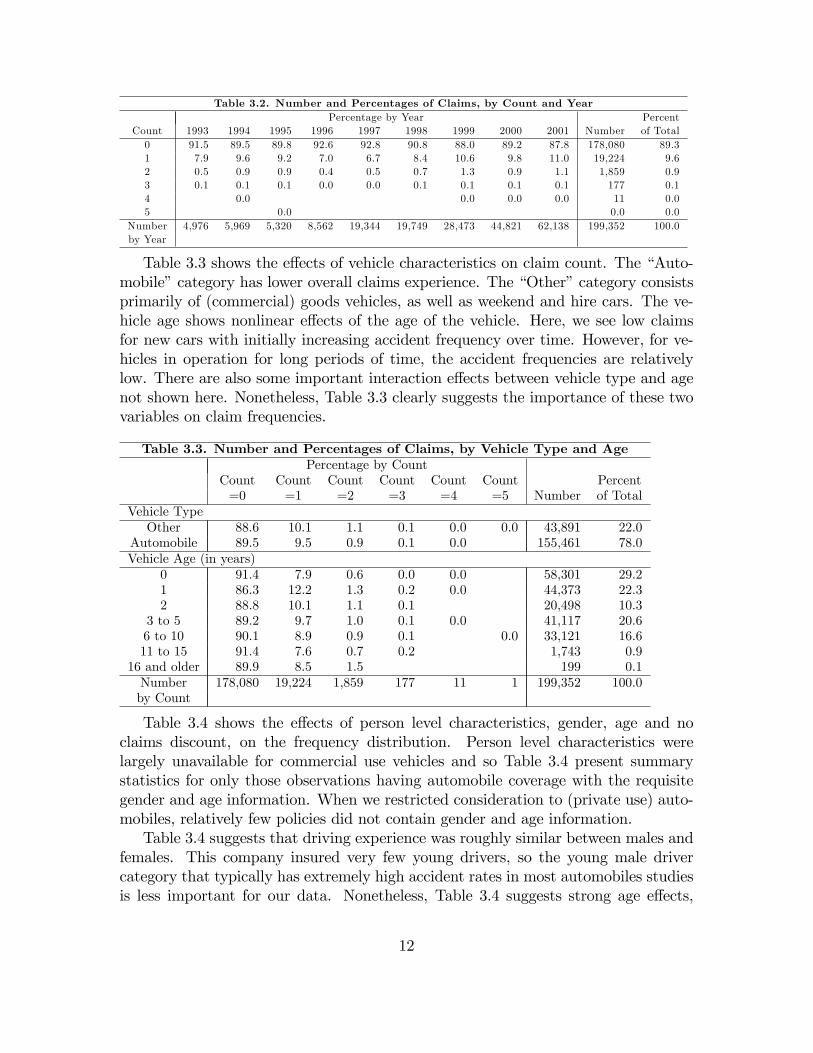
Table 3.2. Number and Percentages of Claims, by Count and YearPercentage by Year Percent

Count 1993 1994 1995 1996 1997 1998 1999 2000 2001 Number of Total0 91.5 89.5 89.8 92.6 92.8 90.8 88.0 89.2 87.8 178,080 89.31 7.9 9.6 9.2 7.0 6.7 8.4 10.6 9.8 11.0 19,224 9.62 0.5 0.9 0.9 0.4 0.5 0.7 1.3 0.9 1.1 1,859 0.93 0.1 0.1 0.1 0.0 0.0 0.1 0.1 0.1 0.1 177 0.14 0.0 0.0 0.0 0.0 11 0.05 0.0 0.0 0.0

Number 4,976 5,969 5,320 8,562 19,344 19,749 28,473 44,821 62,138 199,352 100.0by Year

Table 3.3 shows the e¤ects of vehicle characteristics on claim count. The �Auto-mobile�category has lower overall claims experience. The �Other�category consistsprimarily of (commercial) goods vehicles, as well as weekend and hire cars. The ve-hicle age shows nonlinear e¤ects of the age of the vehicle. Here, we see low claimsfor new cars with initially increasing accident frequency over time. However, for ve-hicles in operation for long periods of time, the accident frequencies are relativelylow. There are also some important interaction e¤ects between vehicle type and agenot shown here. Nonetheless, Table 3.3 clearly suggests the importance of these twovariables on claim frequencies.

Table 3.3. Number and Percentages of Claims, by Vehicle Type and AgePercentage by Count

Count Count Count Count Count Count Percent=0 =1 =2 =3 =4 =5 Number of Total

Vehicle TypeOther 88.6 10.1 1.1 0.1 0.0 0.0 43,891 22.0

Automobile 89.5 9.5 0.9 0.1 0.0 155,461 78.0Vehicle Age (in years)

0 91.4 7.9 0.6 0.0 0.0 58,301 29.21 86.3 12.2 1.3 0.2 0.0 44,373 22.32 88.8 10.1 1.1 0.1 20,498 10.3

3 to 5 89.2 9.7 1.0 0.1 0.0 41,117 20.66 to 10 90.1 8.9 0.9 0.1 0.0 33,121 16.611 to 15 91.4 7.6 0.7 0.2 1,743 0.9

16 and older 89.9 8.5 1.5 199 0.1Number 178,080 19,224 1,859 177 11 1 199,352 100.0by Count

Table 3.4 shows the e¤ects of person level characteristics, gender, age and noclaims discount, on the frequency distribution. Person level characteristics werelargely unavailable for commercial use vehicles and so Table 3.4 present summarystatistics for only those observations having automobile coverage with the requisitegender and age information. When we restricted consideration to (private use) auto-mobiles, relatively few policies did not contain gender and age information.Table 3.4 suggests that driving experience was roughly similar between males and

females. This company insured very few young drivers, so the young male drivercategory that typically has extremely high accident rates in most automobiles studiesis less important for our data. Nonetheless, Table 3.4 suggests strong age e¤ects,

12

with older drivers having better driver experience. Table 3.4 also demonstrates theimportance of the no claims discounts (NCD). As anticipated, drivers with betterprevious driving records enjoy a higher NCD and have fewer accidents. Although notreported here, we also considered interactions among these three variables.

Table 3.4. Number and Percentages of Claims, by Gender, Age and NCDfor Automobile PoliciesPercentage by Count

Count Count Count Count Count Count Percent=0 =1 =2 =3 =4 =5 Number of Total

GenderFemale 89.7 9.3 0.9 0.1 0.0 34,190 22.0Male 89.5 9.5 0.9 0.1 0.0 0.0 121,271 78.0

Person Age (in years)21 and younger 86.9 12.4 0.7 153 0.1

22-25 85.5 12.9 1.4 0.2 3,202 2.126-35 88.0 10.8 1.1 0.1 0.0 0.0 44,134 28.436-45 90.1 9.1 0.8 0.1 0.0 63,135 40.646-55 90.4 8.8 0.8 0.1 0.0 34,373 22.156-65 90.7 8.4 0.9 0.1 9,207 5.9

66 and over 92.8 7.0 0.2 0.1 1,257 0.8No Claims Discount (NCD)

0 87.7 11.1 1.1 0.1 0.0 37,139 23.910 87.8 10.8 1.2 0.1 0.0 13,185 8.520 89.1 9.8 1.0 0.1 14,204 9.130 89.1 10.0 0.9 0.1 12,558 8.140 89.8 9.3 0.9 0.1 0.0 10,540 6.850 91.0 8.3 0.7 0.1 0.0 67,835 43.6

Number 139,183 14,774 1,377 123 3 1 155,461 100.0by Count

As part of the examination process, we investigated interaction terms among thecovariates and nonlinear speci�cations. After additional examination of the data, wereport �ve �tted count models: a basic Poisson model without covariates, Poissonand negative binomial models with covariates, as well as their counterparts thatincorporate random e¤ects. For the latter four models, we used the same covariatesto form the systematic component, x0it��. Maximum likelihood was used to �t eachmodel and empirical Bayes was used to predict the random intercepts.Table 3.5 compares these �ve �tted models, providing predictions for each level of

the response variable. To summarize the overall �t, we report a Pearson chi-squaregoodness of �t statistic. As anticipated, the Poisson performed much better withcovariates, and the negative binomial �t better than the Poisson. Somewhat sur-prisingly, the random e¤ects models fared poorly compared to the negative binomialmodel. However, recall that our data set is from an insurance company where there issubstantial turnover of policies. Thus, we interpret the �ndings of Table 3.5 to meanthat the negative binomial distribution well captures the heterogeneity in the acci-dent frequency distribution and that the no claims discount variable captures claims

13

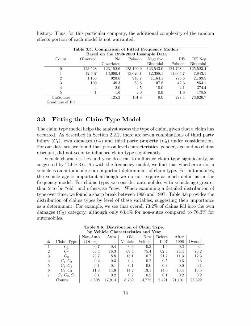
history. Thus, for this particular company, the additional complexity of the randome¤ects portion of each model is not warranted.

Table 3.5. Comparison of Fitted Frequency ModelsBased on the 1993-2000 Insample Data

Count Observed No Poisson Negative RE RE NegCovariates Binomial Poisson Binomial

0 123,528 123,152.6 123,190.9 123,543.0 124,728.4 125,523.41 12,407 13,090.4 13,020.1 12,388.1 11,665.7 7,843.12 1,165 920.6 946.7 1,164.1 775.5 2,189.53 109 48.3 53.6 107.8 42.3 854.14 4 2.0 2.5 10.0 2.1 374.45 1 1.6 2.0 0.9 1.6 178.8

ChiSquare 125.2 101.8 9.0 228.4 73,626.7Goodness of Fit

3.3 Fitting the Claim Type Model

The claim type model helps the analyst assess the type of claim, given that a claim hasoccurred. As described in Section 2.2.2, there are seven combinations of third partyinjury (C1), own damages (C2) and third party property (C3) under consideration.For our data set, we found that person level characteristics, gender, age and no claimsdiscount, did not seem to in�uence claim type signi�cantly.Vehicle characteristics and year do seem to in�uence claim type signi�cantly, as

suggested by Table 3.6. As with the frequency model, we �nd that whether or not avehicle is an automobile is an important determinant of claim type. For automobiles,the vehicle age is important although we do not require as much detail as in thefrequency model. For claims type, we consider automobiles with vehicle age greaterthan 2 to be �old�and otherwise �new.�When examining a detailed distribution oftype over time, we found a sharp break between 1996 and 1997. Table 3.6 provides thedistribution of claims types by level of these variables, suggesting their importanceas a determinant. For example, we see that overall 73.2% of claims fell into the owndamages (C2) category, although only 63.4% for non-autos compared to 76.3% forautomobiles.

Table 3.6. Distribution of Claim Type,by Vehicle Characteristics and Year

Non-Auto Auto Old New Before AfterM Claim Type (Other) Vehicle Vehicle 1997 1996 Overall1 C1 0.7 0.4 0.6 0.3 1.3 0.3 0.42 C2 63.4 76.3 69.4 75.4 62.5 74.4 73.23 C3 23.7 8.8 15.1 10.7 21.2 11.3 12.34 C1; C2 0.2 0.3 0.4 0.2 0.5 0.3 0.35 C1; C3 0.1 0.1 0.1 0.0 0.3 0.0 0.16 C2; C3 11.8 14.0 14.2 13.1 14.0 13.4 13.57 C1; C2; C3 0.1 0.2 0.2 0.2 0.1 0.2 0.2

Counts 5,608 17,914 8,750 14,772 2,421 21,101 23,522

14

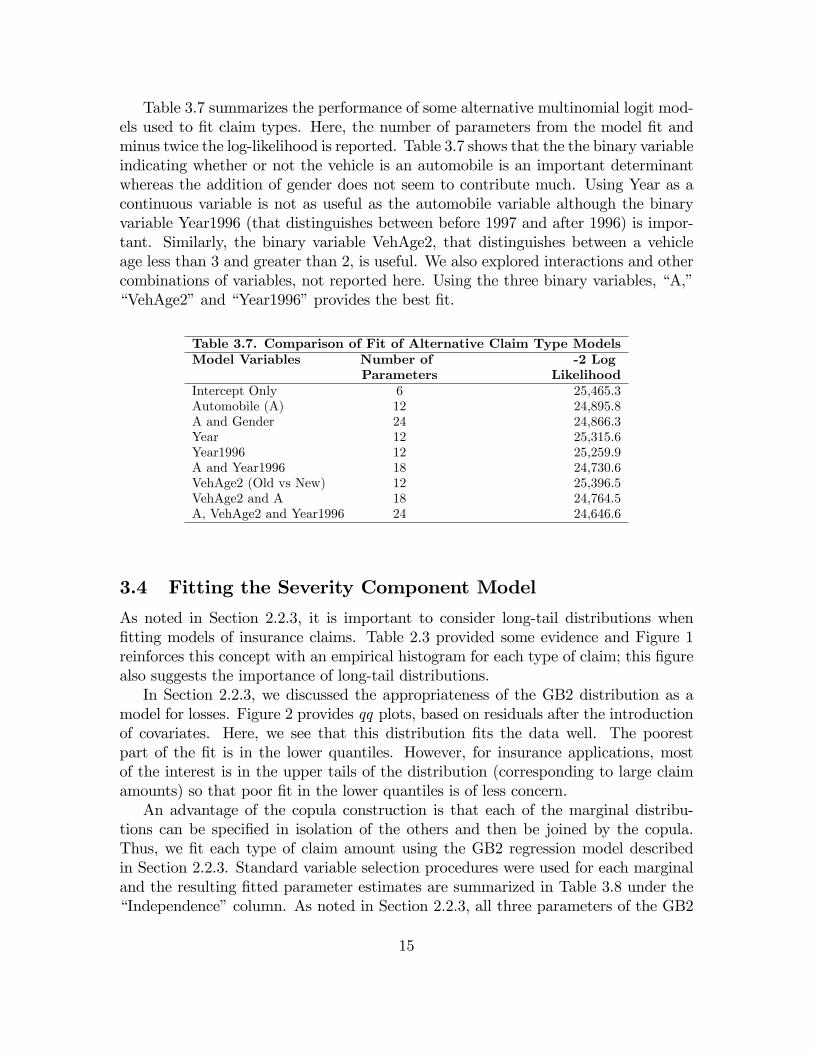
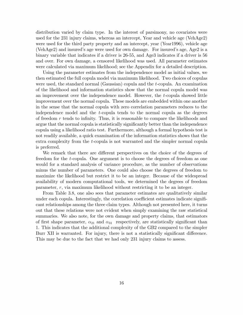
Table 3.7 summarizes the performance of some alternative multinomial logit mod-els used to �t claim types. Here, the number of parameters from the model �t andminus twice the log-likelihood is reported. Table 3.7 shows that the the binary variableindicating whether or not the vehicle is an automobile is an important determinantwhereas the addition of gender does not seem to contribute much. Using Year as acontinuous variable is not as useful as the automobile variable although the binaryvariable Year1996 (that distinguishes between before 1997 and after 1996) is impor-tant. Similarly, the binary variable VehAge2, that distinguishes between a vehicleage less than 3 and greater than 2, is useful. We also explored interactions and othercombinations of variables, not reported here. Using the three binary variables, �A,��VehAge2�and �Year1996�provides the best �t.

Table 3.7. Comparison of Fit of Alternative Claim Type ModelsModel Variables Number of -2 Log

Parameters LikelihoodIntercept Only 6 25,465.3Automobile (A) 12 24,895.8A and Gender 24 24,866.3Year 12 25,315.6Year1996 12 25,259.9A and Year1996 18 24,730.6VehAge2 (Old vs New) 12 25,396.5VehAge2 and A 18 24,764.5A, VehAge2 and Year1996 24 24,646.6

3.4 Fitting the Severity Component Model

As noted in Section 2.2.3, it is important to consider long-tail distributions when�tting models of insurance claims. Table 2.3 provided some evidence and Figure 1reinforces this concept with an empirical histogram for each type of claim; this �gurealso suggests the importance of long-tail distributions.In Section 2.2.3, we discussed the appropriateness of the GB2 distribution as a

model for losses. Figure 2 provides qq plots, based on residuals after the introductionof covariates. Here, we see that this distribution �ts the data well. The poorestpart of the �t is in the lower quantiles. However, for insurance applications, mostof the interest is in the upper tails of the distribution (corresponding to large claimamounts) so that poor �t in the lower quantiles is of less concern.An advantage of the copula construction is that each of the marginal distribu-

tions can be speci�ed in isolation of the others and then be joined by the copula.Thus, we �t each type of claim amount using the GB2 regression model describedin Section 2.2.3. Standard variable selection procedures were used for each marginaland the resulting �tted parameter estimates are summarized in Table 3.8 under the�Independence�column. As noted in Section 2.2.3, all three parameters of the GB2

15

distribution varied by claim type. In the interest of parsimony, no covariates wereused for the 231 injury claims, whereas an intercept, Year and vehicle age (VehAge2)were used for the third party property and an intercept, year (Year1996), vehicle age(VehAge2) and insured�s age were used for own damage. For insured�s age, Age2 is abinary variable that indicates if a driver is 26-55, and Age3 indicates if a driver is 56and over. For own damage, a censored likelihood was used. All parameter estimateswere calculated via maximum likelihood; see the Appendix for a detailed description.Using the parameter estimates from the independence model as initial values, we

then estimated the full copula model via maximum likelihood. Two choices of copulaswere used, the standard normal (Gaussian) copula and the t-copula. An examinationof the likelihood and information statistics show that the normal copula model wasan improvement over the independence model. However, the t-copula showed littleimprovement over the normal copula. These models are embedded within one anotherin the sense that the normal copula with zero correlation parameters reduces to theindependence model and the t-copula tends to the normal copula as the degreesof freedom r tends to in�nity. Thus, it is reasonable to compare the likelihoods andargue that the normal copula is statistically signi�cantly better than the independencecopula using a likelihood ratio test. Furthermore, although a formal hypothesis test isnot readily available, a quick examination of the information statistics shows that theextra complexity from the t-copula is not warranted and the simpler normal copulais preferred.We remark that there are di¤erent perspectives on the choice of the degrees of

freedom for the t-copula. One argument is to choose the degrees of freedom as onewould for a standard analysis of variance procedure, as the number of observationsminus the number of parameters. One could also choose the degrees of freedom tomaximize the likelihood but restrict it to be an integer. Because of the widespreadavailability of modern computational tools, we determined the degrees of freedomparameter, r, via maximum likelihood without restricting it to be an integer.From Table 3.8, one also sees that parameter estimates are qualitatively similar

under each copula. Interestingly, the correlation coe¢ cient estimates indicate signi�-cant relationships among the three claim types. Although not presented here, it turnsout that these relations were not evident when simply examining the raw statisticalsummaries. We also note, for the own damage and property claims, that estimatorsof �rst shape parameter, �21 and �31 respectively, are statistically signi�cant than1. This indicates that the additional complexity of the GB2 compared to the simplerBurr XII is warranted. For injury, there is not a statistically signi�cant di¤erence.This may be due to the fact that we had only 231 injury claims to assess.

16

Table 3.8. Fitted Copula ModelType of Copula

Parameter Independence Normal copula t-copulaThird Party Injury�1 1.316 (0.124) 1.320 (0.138) 1.320 (0.120)�11 2.188 (1.482) 2.227 (1.671) 2.239 (1.447)�12 500.069 (455.832) 500.068 (408.440) 500.054 (396.655)�C;1;1 (intercept) 18.430 (2.139) 18.509 (4.684) 18.543 (4.713)Own Damage�2 1.305 (0.031) 1.301 (0.022) 1.302 (0.029)�21 5.658 (1.123) 5.507 (0.783) 5.532 (0.992)�22 163.605 (42.021) 163.699 (22.404) 170.382 (59.648)�C;2;1 (intercept) 10.037 (1.009) 9.976 (0.576) 10.106 (1.315)�C;2;2 (VehAge2) 0.090 (0.025) 0.091 (0.025) 0.091 (0.025)�C;2;3 (Year1996) 0.269 (0.035) 0.274 (0.035) 0.274 (0.035)�C;2;4 (Age2) 0.107 (0.032) 0.125 (0.032) 0.125 (0.032)�C;2;5 (Age3) 0.225 (0.064) 0.247 (0.064) 0.247 (0.064)Third Party Property�3 0.846 (0.032) 0.853 (0.031) 0.853 (0.031)�31 0.597 (0.111) 0.544 (0.101) 0.544 (0.101)�32 1.381 (0.372) 1.534 (0.402) 1.534 (0.401)�C;3;1 (intercept) 1.332 (0.136) 1.333 (0.140) 1.333 (0.139)�C;3;2 (VehAge2) -0.098 (0.043) -0.091 (0.042) -0.091 (0.042)�C;3;3 (Year1) 0.045 (0.011) 0.038 (0.011) 0.038 (0.011)Copula�12 - 0.018 (0.115) 0.018 (0.115)�13 - -0.066 (0.112) -0.066 (0.111)�23 - 0.259 (0.024) 0.259 (0.024)r - - 193.055 (140.648)Model Fit Statisticslog-likelihood -31,006.505 -30,955.351 -30,955.281number of parms 18 21 22AIC 62,049.010 61,952.702 61,954.562Note: Standard errors are in parenthesis.

4 Inference

As noted in the introduction, an important application of the modeling process forthe actuary involves predicting claims arising from insurance policies. We illustratethe process in two di¤erent ways: (1) prediction based on an individual observationand (2) determination of expected functions of claims over di¤erent policy scenarios.It is common for actuaries to examine one or more �test cases� when setting

premium scales or reserves. The �rst step is to generate a prediction of the claimsfrequency model that we �t in Section 3.2. Because this problem has been welldiscussed in the literature (see, for example, Bolancé et al., 2003), we focus on pre-diction conditional on the occurrence of a claim, that is, N = 1. To illustrate whatan actuary can learn when predicting based on an individual observation, we chose

17

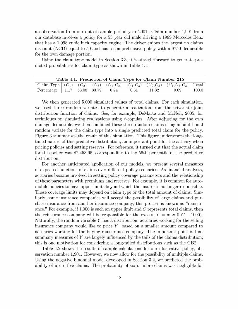
an observation from our out-of-sample period year 2001. Claim number 1,901 fromour database involves a policy for a 53 year old male driving a 1999 Mercedes Benzthat has a 1,998 cubic inch capacity engine. The driver enjoys the largest no claimsdiscount (NCD) equal to 50 and has a comprehensive policy with a $750 deductiblefor the own damage portion.Using the claim type model in Section 3.3, it is straightforward to generate pre-

dicted probabilities for claim type as shown in Table 4.1.

Table 4.1. Prediction of Claim Type for Claim Number 215Claim Type (C 1) (C 2) (C 3) (C 1,C 2) (C 1,C 3) (C 2,C 3) (C 1,C 2,C 3) TotalPercentage 1.17 53.08 33.79 0.24 0.31 11.32 0.09 100.0

We then generated 5,000 simulated values of total claims. For each simulation,we used three random variates to generate a realization from the trivariate jointdistribution function of claims. See, for example, DeMarta and McNeil, 2005, fortechniques on simulating realizations using t-copulas. After adjusting for the owndamage deductible, we then combined these three random claims using an additionalrandom variate for the claim type into a single predicted total claim for the policy.Figure 3 summarizes the result of this simulation. This �gure underscores the long-tailed nature of this predictive distribution, an important point for the actuary whenpricing policies and setting reserves. For reference, it turned out that the actual claimfor this policy was $2,453.95, corresponding to the 56th percentile of the predictivedistribution.For another anticipated application of our models, we present several measures

of expected functions of claims over di¤erent policy scenarios. As �nancial analysts,actuaries become involved in setting policy coverage parameters and the relationshipof these parameters with premiums and reserves. For example, it is common for auto-mobile policies to have upper limits beyond which the insurer is no longer responsible.These coverage limits may depend on claim type or the total amount of claims. Sim-ilarly, some insurance companies will accept the possibility of large claims and pur-chase insurance from another insurance company; this process is known as �reinsur-ance.�For example, if 1,000 is such an upper limit and C represents total claims, thenthe reinsurance company will be responsible for the excess, Y = max(0; C � 1000).Naturally, the random variable Y has a distribution; actuaries working for the sellinginsurance company would like to price Y based on a smaller amount compared toactuaries working for the buying reinsurance company. The important point is thatsummary measures of Y are largely in�uenced by the tails of the claims distribution;this is one motivation for considering a long-tailed distributions such as the GB2.Table 4.2 shows the results of sample calculations for our illustrative policy, ob-

servation number 1,901. However, we now allow for the possibility of multiple claims.Using the negative binomial model developed in Section 3.2, we predicted the prob-ability of up to �ve claims. The probability of six or more claims was negligible for

18

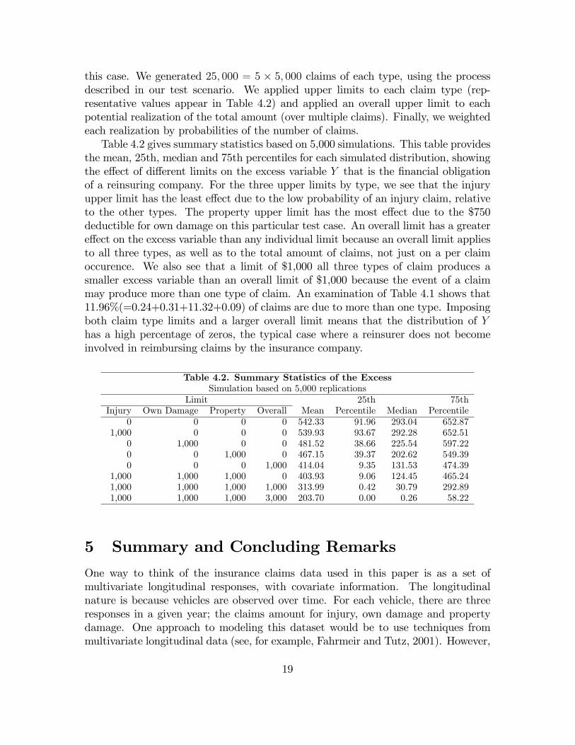
this case. We generated 25; 000 = 5 � 5; 000 claims of each type, using the processdescribed in our test scenario. We applied upper limits to each claim type (rep-resentative values appear in Table 4.2) and applied an overall upper limit to eachpotential realization of the total amount (over multiple claims). Finally, we weightedeach realization by probabilities of the number of claims.Table 4.2 gives summary statistics based on 5,000 simulations. This table provides

the mean, 25th, median and 75th percentiles for each simulated distribution, showingthe e¤ect of di¤erent limits on the excess variable Y that is the �nancial obligationof a reinsuring company. For the three upper limits by type, we see that the injuryupper limit has the least e¤ect due to the low probability of an injury claim, relativeto the other types. The property upper limit has the most e¤ect due to the $750deductible for own damage on this particular test case. An overall limit has a greatere¤ect on the excess variable than any individual limit because an overall limit appliesto all three types, as well as to the total amount of claims, not just on a per claimoccurence. We also see that a limit of $1,000 all three types of claim produces asmaller excess variable than an overall limit of $1,000 because the event of a claimmay produce more than one type of claim. An examination of Table 4.1 shows that11.96%(=0.24+0.31+11.32+0.09) of claims are due to more than one type. Imposingboth claim type limits and a larger overall limit means that the distribution of Yhas a high percentage of zeros, the typical case where a reinsurer does not becomeinvolved in reimbursing claims by the insurance company.

Table 4.2. Summary Statistics of the ExcessSimulation based on 5,000 replications

Limit 25th 75thInjury Own Damage Property Overall Mean Percentile Median Percentile

0 0 0 0 542.33 91.96 293.04 652.871,000 0 0 0 539.93 93.67 292.28 652.51

0 1,000 0 0 481.52 38.66 225.54 597.220 0 1,000 0 467.15 39.37 202.62 549.390 0 0 1,000 414.04 9.35 131.53 474.39

1,000 1,000 1,000 0 403.93 9.06 124.45 465.241,000 1,000 1,000 1,000 313.99 0.42 30.79 292.891,000 1,000 1,000 3,000 203.70 0.00 0.26 58.22

5 Summary and Concluding Remarks

One way to think of the insurance claims data used in this paper is as a set ofmultivariate longitudinal responses, with covariate information. The longitudinalnature is because vehicles are observed over time. For each vehicle, there are threeresponses in a given year; the claims amount for injury, own damage and propertydamage. One approach to modeling this dataset would be to use techniques frommultivariate longitudinal data (see, for example, Fahrmeir and Tutz, 2001). However,

19

as we have pointed out, in most years policyholders do not incur a claim, resulting inmany repeated zeroes (see, for example, Olsen and Shafer, 2001) and, when a claimdoes occur, the distribution is long-tailed. Both of these features are not readilyaccommodated using standard multivariate longitudinal data models that generallyassume data are from an exponential family of distributions.Other possible approaches to modeling the dataset include Bayesian predictive

modeling; see de Alba (2002) and Verrall (2004) for recent actuarial applications.Another approach would be to model the claims count for each of the three typesjointly and thus consider a trivariate Poisson process. This was the approach taken byPinquet (1998) when considering two types of claims, those at fault and no-fault. Thisapproach is comparable to the one taken in this paper in that linear combinationsof Poisson process are also Poisson processes. We have chosen to re-organize thismultivariate count data into count and type events because we feel that this approachis more �exible and easier to implement, especially when the dimension of the typesof claims increases.The main contribution in this paper is the introduction of a multivariate claims

distribution for handling long-tailed, related claims using covariates. We used theGB2 distribution to accommodate the long-tailed nature of claims while at the sametime, allowing for covariates. As an innovative approach, this paper introduces cop-ulas to allow for relationships among di¤erent types of claims.The focus of our illustrations in Section 4 was on predicting total claims arising

from an insurance policy on a vehicle. We also note that our model is su¢ ciently�exible to allow the actuary to focus on a single type of claim. For example, this wouldbe of interest when the actuary is designing an insurance contract and is interested inthe e¤ect of di¤erent deductibles or policy limits on �own damages�types of claims.It is also straightforward to extend this type of calculation to a block of insurancepolicies, such as might be priced in a reinsurance agreement.The modeling approach developed in this paper is su¢ ciently �exible to handle our

complex data. Nonetheless, we acknowledge that many improvements can be made.In particular, we did not investigate potential explanations for the lack of balance inour data; we implicitly assumed that the lack of balance in our longitudinal frameworkwas due to data that were missing at random (Little and Rubin, 1987). It is wellknown in longitudinal data modeling that attrition and other sources of imbalancemay seriously a¤ect statistical inference. This is an area of future investigation.

20

A Appendix - Severity Likelihood

Consider the seven di¤erent combinations of claim types arising when a claim is made.For claim types M = 1; 3; 5, no censoring is involved and we may simply integrateout the e¤ects of the types not observed. Thus, for example, for M = 1; 3, we havethe likelihood contributions to be L1 (c1) = f1 (c1) and L3 (c3) = f3 (c3), respectively.The subscript of the likelihood contribution L refers to the claim type. For claimtypeM = 5, there is also no own damage amount, so that the likelihood contributionis given by

L5 (c1; c3) =

Z 1

0

h3 (F1 (c1) ;F2 (z) ;F3 (c3)) f1 (c1) f3 (c3) f2 (z) dz

= h2 (F1 (c1) ;F3 (c3)) f1 (c1) f3 (c3)

= fuc;13 (c1; c3)

where h2 is the density of the bivariate t-copula, having the same structure as thetrivariate t-copula given in equation (5). Note that we are using the importantproperty that a member of the elliptical family of distributions (and hence ellipticalcopulas) is preserved under the marginals.The cases M = 2; 4; 6; 7 involve own damage claims and so we need to allow for

the possibility of censoring. Let c�2 be the unobserved loss and c2 = max (0; c�2 � d)

be the observed claim. Further de�ne

� =

�1 if c�2 � d0 otherwise

to be a binary variable that indicates censoring. Thus, the familiar M = 2 case is

given by

L2 (c2) =

�f2 (c2 + d) = (1� F2 (d)) if � = 0F2 (d) if � = 1

=

(�f2 (c2 + d)

1� F2 (d)

�1��(F2 (d))

� :

For the M = 6 case, we have

L6 (c2; c3) =

�fuc;23 (c2 + d; c3)

1� F2 (d)

�1��(Hc;23 (d; c3))

�

where

Hc;23 (d; c3) =

Z d

0

h2 (F2 (z) ;F3 (c3)) f3 (c3) f2 (z) dz:

It is not di¢ cult to show that this can also be expressed as

Hc;23 (d; c3) = f3 (c3)H2 (F2 (d) ;F3 (c3)) :

21

TheM = 4 case follows in the same fashion, reversing the roles of types 1 and 3. Themore complex M = 7 case is given by

L7 (c1; c2; c3) =

�fuc;123 (c1; c2 + d; c3)

1� F2 (d)

�1��(Hc;123 (c1; d; c3))

�

where fuc;123 is given in equation (3) and

Hc;123 (c1; d; c3) =

Z d

0

h3 (F1 (c1) ;F2 (z) ;F3 (c3)) f1 (c1) f3 (c3) f2 (z) dz:

With these de�nitions, the total severity log-likelihood for each observational unitis log (LS) =

P7j=1 I (M = j) log (Lj) :

References[1] Angers, Jean-François, Denise Desjardins, Georges Dionne and Francois Guertin (2006). Vehicle

and �eet random e¤ects in a model of insurance rating for �eets of vehicles. ASTIN Bulletin36(1): 25-77.

[2] Antonio, Katrien, Jan Beirlant, Tom Hoedemakers and Robert Verlaak (2006). Lognormalmixed modesl for reported claims reserves. North American Actuarial Journal 10(1): 30�48.

[3] Beirlant, Jan, Yuri Goegebeur, Johan Segers and Jozef Teugels (2004). Statistics of Extremes:Theory and Applications Wiley, New York.

[4] Beirlant, Jan, Yuri Goegebeur, Robert Verlaak and Petra Vynckier (1998). Burr regression andportfolio segmentation. Insurance: Mathematics and Economics 23, 231-250.

[5] Bolancé, Catalina, Montserratt Guillén and Jean Pinquet (2003). Time-varying credibility forfrequency risk models: estimation and tests for autoregressive speci�cations on the randome¤ects. Insurance: Mathematics and Economics 33, 273-282.

[6] Bowers, Newton L., Hans U. Gerber, James C. Hickman, Donald A. Jones and Cecil J. Nesbitt(1997). Actuarial Mathematics. Society of Actuaries, Schaumburg, IL.

[7] Cameron, A. Colin and Pravin K. Trivedi. (1998) Regression Analysis of Count Data. Cam-bridge University Press, Cambridge.

[8] De Alba, Enrique (2002). Bayesian estimation of outstanding claim reserves. North AmericanActuarial Journal 6(4): 1�20.

[9] Demarta, Stefano and Alexander J. McNeil (2005). The t copula and related copulas. Interna-tional Statistical Review 73(1), 111-129.

[10] Desjardins, Denise, Georges Dionne and Jean Pinquet (2001). Experience rating schemes for�eets of vehicles. ASTIN Bulletin 31(1): 81-105.

[11] Diggle, Peter J., Patrick Heagarty, K.-Y. Liang and Scott L. Zeger, (2002). Analysis of Longi-tudinal Data. Second Edition. Oxford University Press.

22

[12] Dionne, Georges and C. Vanasse (1989). A generalization of actuarial automobile insurancerating models: the negative binomial distribution with a regression component. ASTIN Bulletin19, 199-212.

[13] Fahrmeir, Ludwig and Gerhard Tutz. (2001). Multivariate Statistical Modelling Based on Gen-eralized Linear Models. Springer-Verlag.

[14] Frees, Edward W. (2004). Longitudinal and Panel Data: Analysis and Applications for theSocial Sciences. Cambridge University Press.

[15] Frees, Edward W. and Emiliano A. Valdez (1998). Understanding relationships using copulas.North American Actuarial Journal 2(1), 1-25.

[16] Frees, Edward W. and Ping Wang (2005). Credibility using copulas. North American ActuarialJournal 9(2), 31-48.

[17] Jones, AndrewM. (2000). Health econometrics. Chapter 6 of the Handbook of Health Economics,Volume 1. Edited by Antonio.J. Culyer, and Joseph.P. Newhouse, Elsevier, Amersterdam. 265-344.

[18] Klugman, Stuart, Harry Panjer and Gordon Willmot (2004). Loss Models: From Data to De-cisions (Second Edition), Wiley, New York.

[19] Landsman, Zinoviy M. and Emiliano A. Valdez (2003). Tail conditional expectations for ellip-tical distributions. North American Actuarial Journal 7(4), 55-71.

[20] Lemaire, Jean (1985) Automobile Insurance: Actuarial Models, Huebner International Serieson Risk, Insurance and Economic Security, Wharton, Pennsylvania.

[21] Lindskog, Filip and Alexander J. McNeil (2003). Common Poisson shock models: Applicationsto insurance and credit risk modelling. ASTIN Bulletin 33(2): 209�238.

[22] Little, R.J.A., and Rubin, Donald B. (1987). Statistical Analysis with Missing Data. New York,NY: Wiley.

[23] McCullagh, Peter and John A. Nelder (1989). Generalized Linear Models (Second Edition).Chapman and Hall, London.

[24] McDonald, James B. and Richard J. Butler (1990). Regression models for positive randomvariables.Journal of Econometrics 43, 227-251.

[25] McDonald, James B. and Yexiao J. Xu (1995). A generalization of the beta distribution withapplications. Journal of Econometrics 66, 133-152.

[26] Nelsen, Roger (1999). An Introduction to Copulas. Springer, New York.

[27] Olsen, Maren K. and Joseph L. Shafer (2001). A two-part random-e¤ects model for semicon-tinuous longitudinal data. Journal of the American Statistical Association 96, 730-745.

[28] Pinquet, Jean (1997). Allowance for cost of claims in bonus-malus systems. ASTIN Bulletin27(1): 33�57.

[29] Pinquet, Jean (1998). Designing optimal bonus-malus systems from di¤erent types of claims.ASTIN Bulletin 28(2): 205-229.

23

[30] Pinquet, Jean (2000). Experience rating through heterogeneous models. In Handbook of Insur-ance, editor by G. Dionne. Kluwer Academic Publishers.

[31] Pinquet, Jean, Montserratt Guillén and Catalina Bolancé (2001). Allowance for age of claimsin bonus-malus systems. ASTIN Bulletin 31(2): 337-348.

[32] Purcaru, Oana and Michel Denuit (2003). Dependence in dynamic claim frequency credibilitymodels. ASTIN Bulletin 33(1), 23-40.

[33] Sun, Jiafeng, Edward W. Frees and Marjorie A. Rosenberg (2007). Heavy-tailed longitu-dinal data modeling using copulas. University of Wisconsin working paper, available athttp://research3.bus.wisc.edu/course/view.php?id=129.

[34] Verrall, Richard J. (2004). A Bayesian generalized linear model for the Bornhuetter-Fergusonmethod of claims reserving. North American Actuarial Journal 8(3): 67�89.

Author information:

Edward W. FreesSchool of BusinessUniversity of WisconsinMadison, Wisconsin 53706 USAe-mail: jfrees@bus.wisc.edu

Emiliano A. ValdezSchool of Actuarial StudiesFaculty of Commerce & EconomicsUniversity of New South WalesSydney, Australia 2052e-mail: e.valdez@unsw.edu.au

24

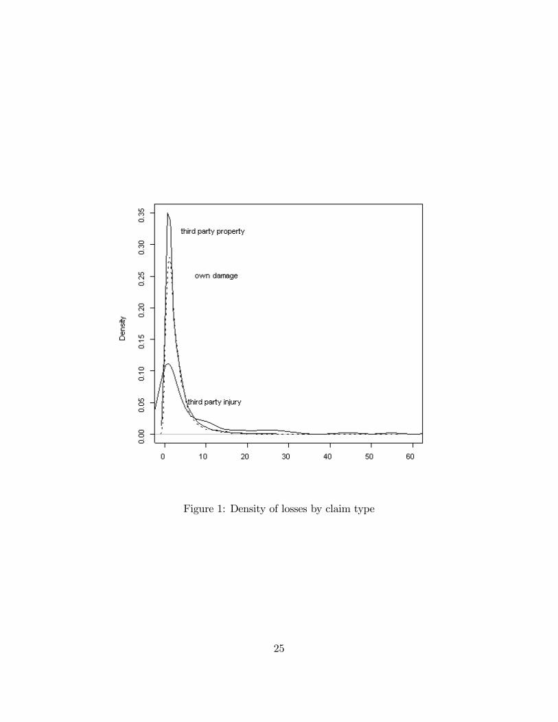
Figure 1: Density of losses by claim type

25

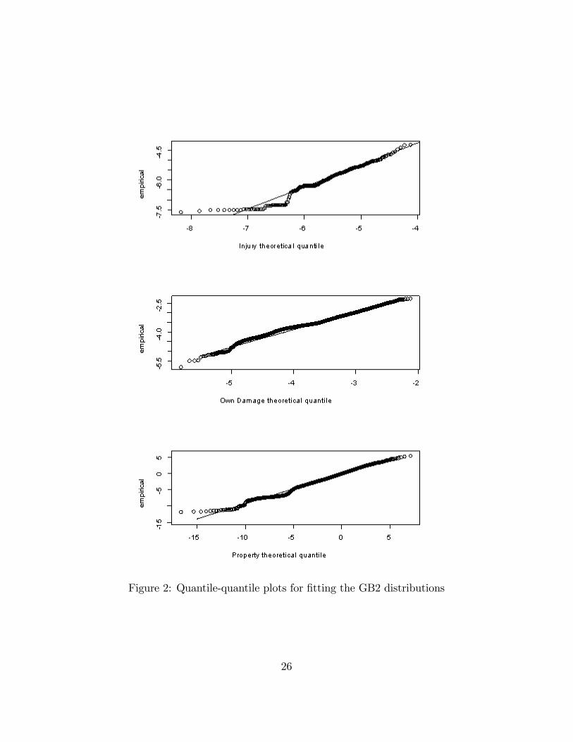
Figure 2: Quantile-quantile plots for �tting the GB2 distributions

26

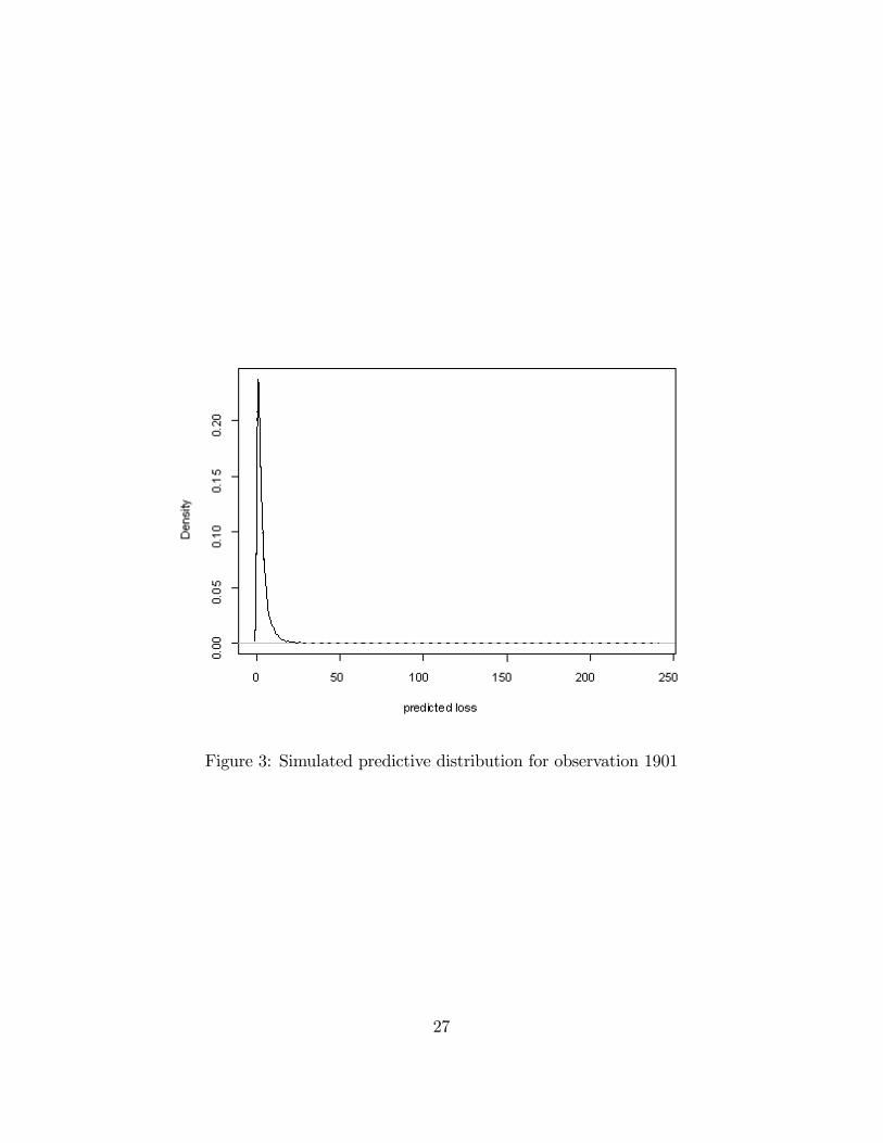
Figure 3: Simulated predictive distribution for observation 1901

27