Hierarchical Matrix Computations:GPU Implementations and Applications

George TurkiyyahKAUST and American University of Beirut

Workshop on Scalable Hierarchical Algorithms for Extreme ComputingMay 9, 2016

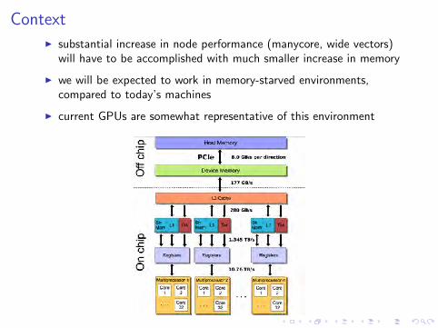
ContextI substantial increase in node performance (manycore, wide vectors)

will have to be accomplished with much smaller increase in memory

I we will be expected to work in memory-starved environments,compared to today’s machines

I current GPUs are somewhat representative of this environment

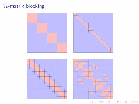
H-matrix blocking

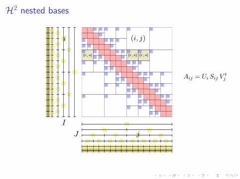
H2 nested bases

I

J

(i, j)i

j

(r,∗) (r,∗) (r,∗)

Aij = Ui Sij Vtj

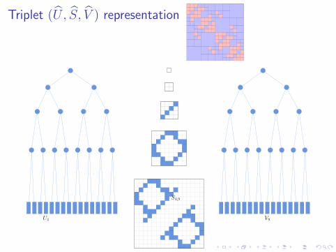
Triplet (U , S, V ) representation

V9

S4,9

U4

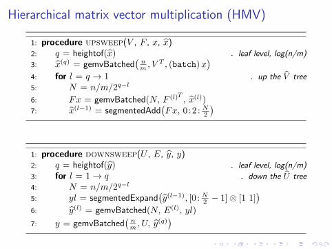
Hierarchical matrix vector multiplication (HMV)

1: procedure upsweep(V , F , x, x)2: q = heightof(x) . leaf level, log(n/m)

3: x(q) = gemvBatched(nm , V

T , (batch)x)

4: for l = q → 1 . up the V tree

5: N = n/m/2q−l

6: Fx = gemvBatched(N, F (l)T , x(l))7: x(l−1) = segmentedAdd

(Fx, 0:2 : N2

)

1: procedure downsweep(U , E, y, y)2: q = heightof(y) . leaf level, log(n/m)

3: for l = 1→ q . down the U tree

4: N = n/m/2q−l

5: yl = segmentedExpand(y(l−1), [0 : N2 − 1]⊗ [1 1]

)

6: y(l) = gemvBatched(N, E(l), yl)

7: y = gemvBatched(nm , U, y

(q))

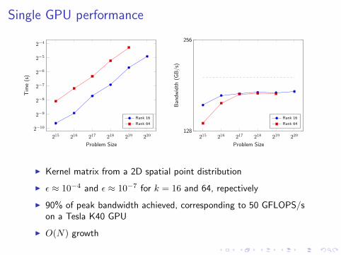
Single GPU performance

215 216 217 218 219 220

2−10

2−9

2−8

2−7

2−6

2−5

2−4

Problem Size

Tim

e(s

)

Rank 16

Rank 64

215 216 217 218 219 220128

256

Problem Size

Ban

dw

idth

(GB

/s)

Rank 16

Rank 64

I Kernel matrix from a 2D spatial point distribution

I ε ≈ 10−4 and ε ≈ 10−7 for k = 16 and 64, repectively

I 90% of peak bandwidth achieved, corresponding to 50 GFLOPS/son a Tesla K40 GPU

I O(N) growth

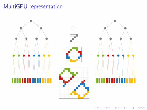
MultiGPU representation

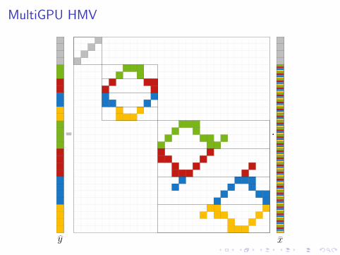
MultiGPU HMV

= ·

y x

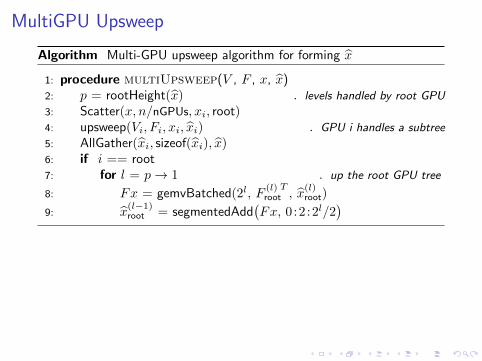
MultiGPU Upsweep

Algorithm Multi-GPU upsweep algorithm for forming x

1: procedure multiUpsweep(V , F , x, x)2: p = rootHeight(x) . levels handled by root GPU

3: Scatter(x, n/nGPUs, xi, root)4: upsweep(Vi, Fi, xi, xi) . GPU i handles a subtree

5: AllGather(xi, sizeof(xi), x)6: if i == root7: for l = p→ 1 . up the root GPU tree

8: Fx = gemvBatched(2l, F(l)root

T, x

(l)root)

9: x(l−1)root = segmentedAdd

(Fx, 0:2 :2l/2

)

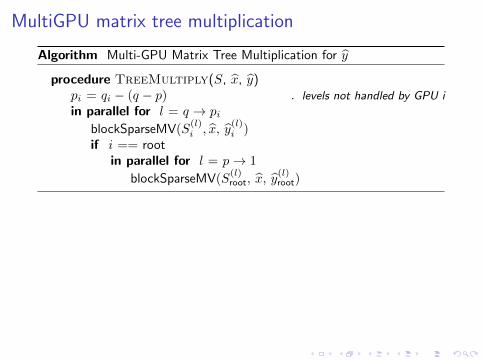
MultiGPU matrix tree multiplication

Algorithm Multi-GPU Matrix Tree Multiplication for y

procedure TreeMultiply(S, x, y)pi = qi − (q − p) . levels not handled by GPU i

in parallel for l = q → piblockSparseMV(S

(l)i , x, y

(l)i )

if i == rootin parallel for l = p→ 1

blockSparseMV(S(l)root, x, y

(l)root)

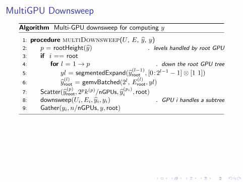
MultiGPU Downsweep

Algorithm Multi-GPU downsweep for computing y

1: procedure multiDownsweep(U , E, y, y)2: p = rootHeight(y) . levels handled by root GPU

3: if i == root4: for l = 1→ p . down the root GPU tree

5: yl = segmentedExpand(y(l−1)root , [0 :2l−1 − 1]⊗ [1 1])

6: y(l)root = gemvBatched(2l, E

(l)root, yl)

7: Scatter(y(p)root, 2

pk(p)/nGPUs, y(pi)i , root)

8: downsweep(Ui, Ei, yi, yi) . GPU i handles a subtree

9: Gather(yi, n/nGPUs, y, root)

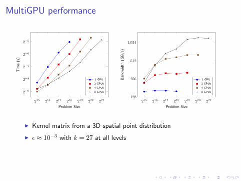
MultiGPU performance

215 216 217 218 219 220 221

2−9

2−8

2−7

2−6

2−5

Problem Size

Tim

e(s

)

1 GPU

2 GPUs

4 GPUs

8 GPUs

215 216 217 218 219 220 221128

256

512

1,024

Problem Size

Ban

dw

idth

(GB

/s)

1 GPU

2 GPUs

4 GPUs

8 GPUs

I Kernel matrix from a 3D spatial point distribution

I ε ≈ 10−3 with k = 27 at all levels

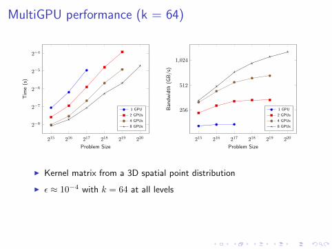
MultiGPU performance (k = 64)

215 216 217 218 219 220

2−8

2−7

2−6

2−5

2−4

Problem Size

Tim

e(s

)

1 GPU

2 GPUs

4 GPUs

8 GPUs

215 216 217 218 219 220

256

512

1,024

Problem Size

Ban

dw

idth

(GB

/s)

1 GPU

2 GPUs

4 GPUs

8 GPUs

I Kernel matrix from a 3D spatial point distribution

I ε ≈ 10−4 with k = 64 at all levels

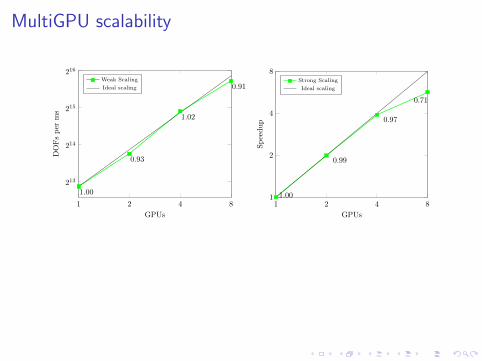
MultiGPU scalability

1 2 4 8

213

214

215

216

1.00

0.93

1.02

0.91

GPUs

DOFsper

ms

Weak Scaling

Ideal scaling

1 2 4 81

2

4

8

1.00

0.99

0.97

0.71

GPUs

Speedup

Strong Scaling

Ideal scaling

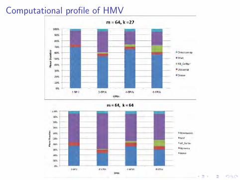
Computational profile of HMV

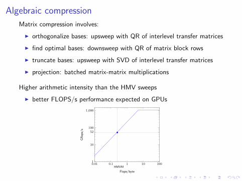
Algebraic compression

Matrix compression involves:

I orthogonalize bases: upsweep with QR of interlevel transfer matrices

I find optimal bases: downsweep with QR of matrix block rows

I truncate bases: upsweep with SVD of interlevel transfer matrices

I projection: batched matrix-matrix multiplications

Higher arithmetic intensity than the HMV sweeps

I better FLOPS/s performance expected on GPUs

0.01 0.1 1 10 1001

10

100

1,000

HMVM

52

Flops/byte

Gfl

ops/

s

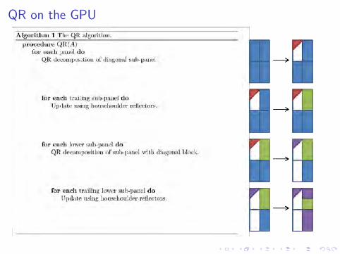
QR on the GPU

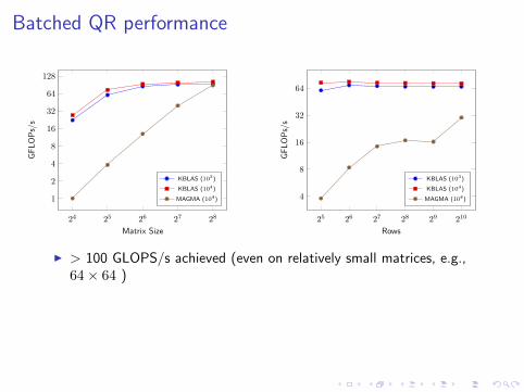
Batched QR performance

24 25 26 27 28

1

2

4

8

16

32

64

128

Matrix Size

GF

LO

Ps/

s

KBLAS (103)

KBLAS (104)

MAGMA (104)

25 26 27 28 29 210

4

8

16

32

64

Rows

GF

LO

Ps/

s

KBLAS (103)

KBLAS (104)

MAGMA (104)

I > 100 GLOPS/s achieved (even on relatively small matrices, e.g.,64× 64 )

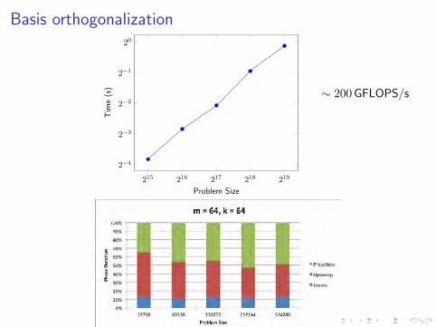
Basis orthogonalization

215 216 217 218 219

2−4

2−3

2−2

2−1

20

Problem Size

Tim

e(s

) ∼ 200 GFLOPS/s

High dimensional integration

Multivariate normal integration:

Φn(a, b; Σ) =

∫ b

a

φn(x; Σ) dx

=1√

|Σ|(2π)n

∫ b1

a1

∫ b2

a2

. . .

∫ bn

an

e−12x

tΣ−1x dxn · · · dx1

Computational approaches when d is moderate to high:

I Monte Carlo methods

I quasi-Monte Carlo

I sparse grids

Seek to exploit a hierarchical structure of the covariance matrix tocompute approximations of the MVN integral efficiently.

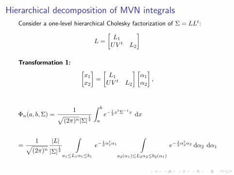
Hierarchical decomposition of MVN integrals

Consider a one-level hierarchical Cholesky factorization of Σ = LLt:

L =

[L1

UV t L2

]

Transformation 1:[x1

x2

]=

[L1

UV t L2

] [α1

α2

],

Φn(a, b,Σ) =1

√(2π)n|Σ| 12

∫ b

a

e−12x

tΣ−1x dx

=1√

(2π)n|L||Σ| 12

∫

a1≤L1α1≤b1

e−12α

t1α1

∫

a2(α1)≤L2α2≤b2(α1)

e−12α

t2α2 dα2 dα1

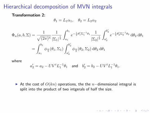
Hierarchical decomposition of MVN integrals

Transformation 2:θ1 = L1α1, θ2 = L2α2

Φn(a, b,Σ) =1√

(2π)n1

|Σ1|12

∫ b1

a1

e−12 θ

t1Σ−1

1 θ11

|Σ2|12

∫ b′2

a′2

e−12 θ

t2Σ−1

2 θ2 dθ2 dθ1

=

∫ b1

a1

φn2

(θ1,Σ1)

∫ b′2

a′2

φn2

(θ2,Σ2) dθ2 dθ1

wherea′2 = a2 − UV tL−1

1 θ1 and b′2 = b2 − UV tL−11 θ1.

I At the cost of O(kn) operations, the the n−dimensional integral issplit into the product of two intgerals of half the size.

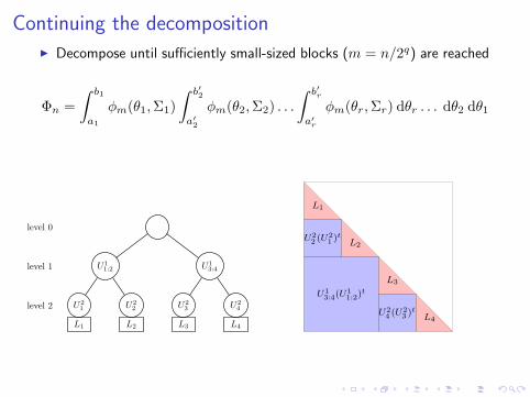
Continuing the decompositionI Decompose until sufficiently small-sized blocks (m = n/2q) are reached

Φn =

∫ b1

a1

φm(θ1,Σ1)

∫ b′2

a′2

φm(θ2,Σ2) . . .

∫ b′r

a′r

φm(θr,Σr) dθr . . . dθ2 dθ1

U11:2

U21 U2

2

U13:4

U23 U2

4

L1 L2 L3 L4

level 0

level 1

level 2

L1

L2

L3

L4

U22 (U

21 )

t

U24 (U

23 )

t

U13:4(U

11:2)

t

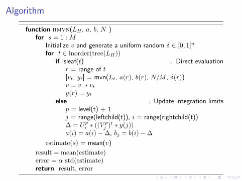
Algorithm

function hmvn(LH , a, b, N )for s = 1 : M

Initialize v and generate a uniform random δ ∈ [0, 1]n

for t ∈ inorder(tree(LH))if isleaf(t) . Direct evaluation

r = range of t[vt, yt] = mvn(Lt, a(r), b(r), N/M , δ(r))v = v. ∗ vty(r) = yt

else . Update integration limitsp = level(t) + 1j = range(leftchild(t)), i = range(rightchild(t))∆ = Upi ∗ ((V pj )t ∗ y(j))a(i) = a(i)−∆, bj = b(i)−∆

estimate(s) = mean(v)

result = mean(estimate)error = α std(estimate)return result, error

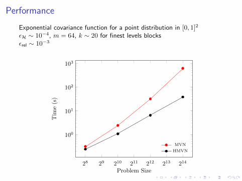
Performance

Exponential covariance function for a point distribution in [0, 1]2

εH ∼ 10−4, m = 64, k ∼ 20 for finest levels blocksεrel ∼ 10−3

28 29 210 211 212 213 214

100

101

102

103

Problem Size

Tim

e(s)

MVN

HMVN

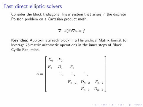
Fast direct elliptic solvers

Consider the block tridiagonal linear system that arises in the discretePoisson problem on a Cartesian product mesh.

∇ · κ(~x)∇u = f

Key idea: Approximate each block in a Hierarchical Matrix format toleverage H-matrix arithmetic operations in the inner steps of BlockCyclic Reduction.

A =

D0 F0

E1 D1 F1

. . .. . .

. . .

En−2 Dn−2 Fn−2

En−1 Dn−1

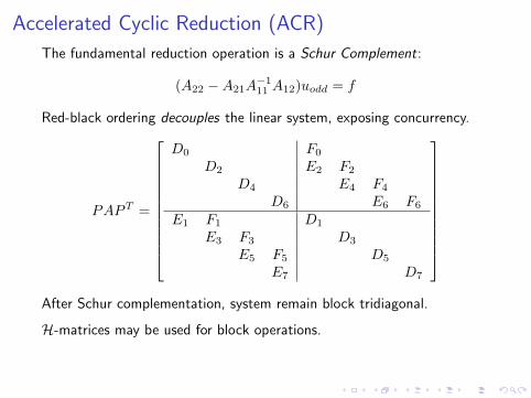
Accelerated Cyclic Reduction (ACR)

The fundamental reduction operation is a Schur Complement:

(A22 −A21A−111 A12)uodd = f

Red-black ordering decouples the linear system, exposing concurrency.

PAPT =

D0 F0

D2 E2 F2

D4 E4 F4

D6 E6 F6

E1 F1 D1

E3 F3 D3

E5 F5 D5

E7 D7

After Schur complementation, system remain block tridiagonal.

H-matrices may be used for block operations.

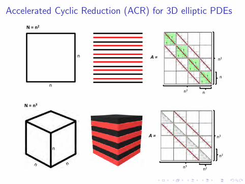
Accelerated Cyclic Reduction (ACR) for 3D elliptic PDEs

N = n3

n

n2

n2

n3

n3

A =

n

n

N = n2

A =

n

n

n2

n2

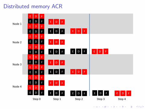
Distributed memory ACR

E

E

E

E

E

E

F

F

F

F

F

F

D

D

D

D

D

D

Step 0 Step 1 Step 2 Step 3 Step 4

E

E

E

E

E

E

F

F

F

F

F

F

D

D

D

D

D

D

E

E

E

E

F

F

F

F

D

D

D

D

E

E

E

F

F

F

D

D

D

E

E

E

F

F

F

D

D

D

E

E

F

F

D

D

E

E

F

F

D

D

E

E

F

F

D

D

E

E

F

F

D

D E F D

Node 1 Node 2 Node 3 Node 4

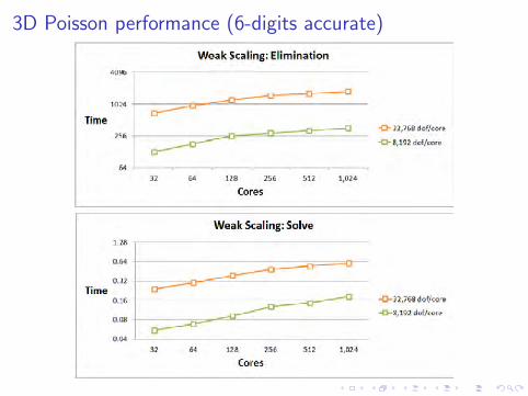
3D Poisson performance (6-digits accurate)

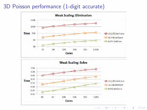
3D Poisson performance (1-digit accurate)

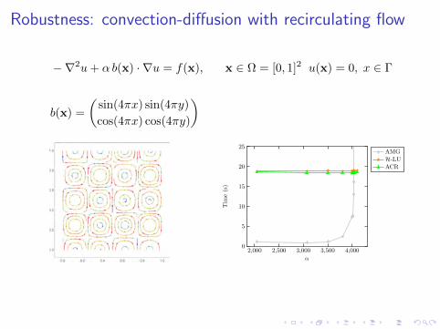
Robustness: convection-diffusion with recirculating flow

−∇2u+ α b(x) · ∇u = f(x), x ∈ Ω = [0, 1]2 u(x) = 0, x ∈ Γ

b(x) =

(sin(4πx) sin(4πy)

cos(4πx) cos(4πy)

)

2,000 2,500 3,000 3,500 4,0000

5

10

15

20

25

α

Tim

e(s)

AMGH-LUACR

ConclusionsI H2 computations are amenable to efficient processing on GPUs

I open the door for many interesting applications