Hierarchical Structure of Magnetohydrodynamic Turbulence in Position-Position-Velocity Space

CitationBurkhart, Blakesley, A. Lazarian, Alyssa A. Goodman, and Erik Rosolowsky. 2013. “Hierarchical structure of magnetohydrodynamic turbulence in position-position-velocity space.” Astrophysical Journal 770 (2) (June 20): 141. doi:10.1088/0004-637X/770/2/141. http://dx.doi.org/10.1088/0004-637X/770/2/141.

Published Versiondoi:10.1088/0004-637X/770/2/141

Permanent linkhttp://nrs.harvard.edu/urn-3:HUL.InstRepos:11688784

Terms of UseThis article was downloaded from Harvard University’s DASH repository, and is made available under the terms and conditions applicable to Open Access Policy Articles, as set forth at http://nrs.harvard.edu/urn-3:HUL.InstRepos:dash.current.terms-of-use#OAP

Share Your StoryThe Harvard community has made this article openly available.Please share how this access benefits you. Submit a story .

Accessibility

arX

iv:1

206.

4703

v1 [

astr

o-ph

.GA

] 2

0 Ju

n 20

12Draft version June 22, 2012Preprint typeset using LATEX style emulateapj v. 5/2/11

HIERARCHICAL STRUCTURE OF MAGNETOHYDRODYNAMIC TURBULENCE INPOSITION-POSITION-VELOCITY SPACE

Blakesley Burkhart1, A. Lazarian1, Alyssa Goodman2, Erik Rosolowsky3

Draft version June 22, 2012

ABSTRACT

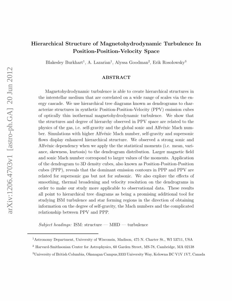
Magnetohydrodynamic turbulence is able to create hierarchical structures in the interstellar mediumthat are correlated on a wide range of scales via the energy cascade. We use hierarchical tree diagramsknown as dendrograms to characterize structures in synthetic Position-Position-Velocity (PPV) emis-sion cubes of optically thin isothermal magnetohydrodynamic turbulence. We show that the structuresand degree of hierarchy observed in PPV space are related to the physics of the gas, i.e. self-gravityand the global sonic and Alfvenic Mach number. Simulations with higher Alfvenic Mach number,self-gravity and supersonic flows display enhanced hierarchical structure. We observed a strong sonicand Alfvenic dependency when we apply the the statistical moments (i.e. mean, variance, skewness,kurtosis) to the dendrogram distribution. Larger magnetic field and sonic Mach number correspondto larger values of the moments. Application of the dendrogram to 3D density cubes, also knownas Position-Position-Position cubes (PPP), reveals that the dominant emission contours in PPP andPPV are related for supersonic gas but not for subsonic. We also explore the effects of smoothing,thermal broadening and velocity resolution on the dendrograms in order to make our study moreapplicable to observational data. These results all point to hierarchical tree diagrams as being apromising additional tool for studying ISM turbulence and star forming regions in the direction of ob-taining information on the degree of self-gravity, the Mach numbers and the complicated relationshipbetween PPV and PPP.Subject headings: ISM: structure — MHD — turbulence

1. INTRODUCTION

The current understanding of the interstellar medium(ISM) is that it is a multi-phase environment com-posed of a tenuous plasma, consisting of gas and dust,which is both magnetized and highly turbulent (Ferriere2001; McKee & Ostriker 2007). In particular, magneto-hydrodynamic (MHD) turbulence is essential to manyastrophysical phenomena such as star formation, cos-mic ray dispersion, and many transport processes. (seeElmegreen & Scalo 2004; Ballesteros-Paredes et al. 2007and references therein). Additionally, turbulence has theunique ability to transfer energy over scales ranging fromkiloparsecs down to the proton gyroradius. This is criti-cal for the ISM, as it explains how energy is distributedfrom large to small spatial scales in the Galaxy.Observationally, several techniques exist to study

MHD turbulence in different ISM phases. Many of thesetechniques focus on the density fluctuations in ionizedmedia (Armstrong et al. 1995; Chepurnov & Lazar-ian 2010), fluctuations in spectroscopic data and columndensity maps for neutral media (Spangler & Gwinn 1990;Padoan et al. 2003) , or gradients of linear polarizationmaps (Haverkorn & Heitsch 2004; Gaensler et al. 2011;Burkhart, Lazarian & Gaensler 2012). For studies ofturbulence, spectroscopic data has a clear advantage inthat it contains information about the turbulent veloc-ity field as well as the density fluctuations. However,

1 Astronomy Department, University of Wisconsin, Madison,475 N. Charter St., WI 53711, USA

2 Harvard-Smithsonian Center for Astrophysics, 60 GardenStreet, MS-78, Cambridge, MA 02138

3 University of British Columbia, Okanagan Campus,3333University Way, Kelowna BC V1V 1V7, Canada

density and velocity are entangled in PPV space, mak-ing the interpretation of this type of data difficult. Forthe separation of the density and velocity fluctuations,special techniques such as the Velocity Coordinate Spec-trum (VCS) and the Velocity Channel Analysis (VCA)have been developed (Lazarian & Pogosyan 2000, 2004,2006, 2008).Most of the efforts to relate observations and simula-

tions of magnetized turbulence are based on obtainingthe spectral index (i.e. the log-log slope of the powerspectrum) of either the density and/or velocity (Lazarian& Esquivel 2003; Esquivel & Lazarian 2005; Ossenkopfet al. 2006). However, the power spectrum alone doesnot provide a full description of turbulence, as it onlycontains the Fourier amplitudes and neglects informa-tion on phases. This fact combined with the knowledgethat astrophysical turbulence is complex, with multipleinjection scales occurring in a multiphase medium, pointsto researchers needing additional ways of analyzing ob-servational and numerical data in the context of turbu-lence. In particular these technique studies are currentlyfocused into two categories:

• Development: Test and develop techniques thatwill complement and build off of the theoreticaland practical picture of a turbulent ISM that thepower spectrum presents.

• Synergy: Use several techniques simultaneously toobtain an accurate picture of the parameters of tur-bulence in the observations.

In regards to the first point, there has been substan-tial progress in the development of techniques to studyturbulence in the last decade. Techniques for the study

2 BURKHART ET AL.

of turbulence can be tested empirically using parameterstudies of numerical simulations or with the aid of ana-lytical predictions (as was done in the case of VCA). Inthe former, the parameters to be varied (see Burkhart& Lazarian 2011) include the Reynolds number, sonicand Alfvenic Mach number, injection scale, equation ofstate, and, for studies of molecular clouds, should in-clude radiative transfer and self-gravity (see Ossenkopf2002; Padoan et al. 2003; Goodman et al. 2009). Somerecently developed techniques include the applicationof probability distribution functions (PDFs), wavelets,spectral correlation function (SCF),4 delta-variance, theprincipal component analysis, higher order moments,Genus, Tsallis statistics, spectrum and bispectrum (Gill& Henriksen 1990; Stutzki et al. 1998; Rosolowsky etal. 1999; Brunt & Heyer 2002; Kowal, Lazarian & Beres-nyak 2007; Chepurnov et al. 2008; Burkhart et al. 2009;Esquivel & Lazarian 2010; Tofflemire et al. 2011). Addi-tionally, these techniques are being tested and applied todifferent wavelengths and types of data. For example, thePDFs and their mathematical descriptors have been ap-plied to the observations in the context of turbulence innumerous works using different data sets including: lin-ear polarization data (see Gaensler et al. 2011; Burkhart,Lazarian, & Gaensler 2012), HI column density of theSMC (Burkhart et al. 2010), molecular/ dust extinctionmaps (Goodman, Pineda, & Schnee 2009; Brunt 2010;Kainulainen et al. 2011) and emission measure and vol-ume averaged density in diffuse ionized gas (Hill et al.2008; Berkhuijsen & Fletcher 2008).The latter point in regard to the synergetic use of tools

for ISM turbulence is only recently being attempted asmany techniques are still in the stages of being devel-oped. However, this approach was used in Burkhart etal. 2010, which applied spectrum, bispectrum and higherorder moments to H I column density of the SMC. Theconsistency of results obtained with a variety of statis-tics and compared with more traditional observationalmethods made this study of turbulence in the SMC apromising first step.This paper falls under the category of “technique de-

velopment.” In particular, we investigate the utility ofdendrograms in studying the hierarchical structure ofISM clouds. It has long been known that turbulence isable to create hierarchical structures in the ISM (Scalo1985, 1990; Vazquez-Semadeni 1993 ;Stutzki 1998), how-ever many questions remain, such as what type of turbu-lence is behind the creation of this hierarchy and whatis the role of self-gravity and magnetic fields? Hierar-chical structure in relation to these questions is particu-larly important for the star formation problem (Larson1981; Elmegreen & Elmegreen 1983; Feitzinger & Galin-ski 1987; Elmegreen 2011).The earliest attempts to characterize ISM hierarchy

utilized tree diagrams as a mechanism for reducing thedata down to hierarchical ’skeleton images’ (see Houla-han & Scalo 1992). More recently dendrograms havebeen used on ISM data in order to characterize self-gravitating structures in star forming molecular clouds(Rosolowsky et al. 2008 and Goodman et al. 2009). Adendrogram (from the Greek dendron “tree”,- gramma

4 The similarities between VCA and SCF are discussed in Lazar-ian (2009).

“drawing”) is a hierarchical tree diagram that has beenused extensively in other fields, particularly in computa-tional biology, and occasionally in galaxy evolution (seeSawlaw & Haque-Copilah 1998 and Podani, Engloner, &Major 2009 for examples). Rosolowsky et al. (2008) andGoodman et al. (2009) used the dendrogram on spec-tral line data of L1448 to estimate key physical proper-ties associated with isosurfaces of local emission maximasuch as radius, velocity dispersion, and luminosity. Theseworks provided a new and promising way of character-izing self-gravitating structures and properties of molec-ular clouds through the application of dendrogram to13CO(J=1-0) PPV data.In this paper we apply the dendrogram to synthetic ob-

servations (specifically PPV cubes) of isothermal MHDturbulence in order to investigate the physical mecha-nisms behind the gas hierarchy. Additionally, we are in-terested in the nature of the structures that are found inPPV data and how these structures are related to boththe physics of the gas and the underlying density and ve-locity fluctuations generated by turbulence. Simulationsprovide an excellent testing ground for this problem, asone can identify which features in PPV space are den-sity features and which are caused by velocity crowding.Furthermore, one can answer the question of under whatconditions do the features in PPV relate back to the 3Ddensity or PPP cube?In order to answer these questions we perform a pa-

rameter study using the dendrogram. We focus on howchanging the global parameters of the turbulence, suchas the sonic Mach number, Alfvenic Mach number andlevel of self-gravity affect the amount of hierarchy ob-served, the relationship between the density and velocitystructures in PPV, and the number and statistical distri-bution of dominate emission structures. Along with theReynolds number, the sonic and Alfvenic Mach numbersare useful descriptors of the turbulence and are critical toseveral phenomena in astrophysics, including cosmic rayacceleration, turbulent magnetic reconnection, ambipo-lar diffusion and structure formation in the ISM. Theyare defined as the ratio of the flow velocity to the soundspeed and Alfven speed, respectively. That is, the sonicMach number is Ms ≡ VL/cs, where VL is the injectionvelocity, cs is the sound velocity, and the Alfvenic Machnumber is MA ≡ VL/VA, where VA is the Alfven veloc-ity. The Sonic Mach number provides important clues onthe role of fluid compressibility while the Alfvenic Machnumber gives insight into the influence of the magneticfield in the evolution of ISM turbulence. Throughout thepaper we will use the terms “compressibility“ and SonicMach number interchangeably.The paper is organized as follows. In § 2 we describe

the dendrogram algorithm, in § 3 we discuss the simula-tions and provide a description of the MHD models. Weinvestigate the physical mechanisms that create hierar-chical structure in the dendrogram tree and as well ascharacterize the tree diagrams via statistical moments in§ 4. In § 5 we compare the dendrograms of PPP andPPV. In § 6 we discuss application and investigate is-sues of resolution. Finally, in § 7 we discuss our resultsfollowed by the conclusions in § 8.

2. DENDROGRAM ALGORITHM

Hierarchical Structure of MHD Turbulence 3

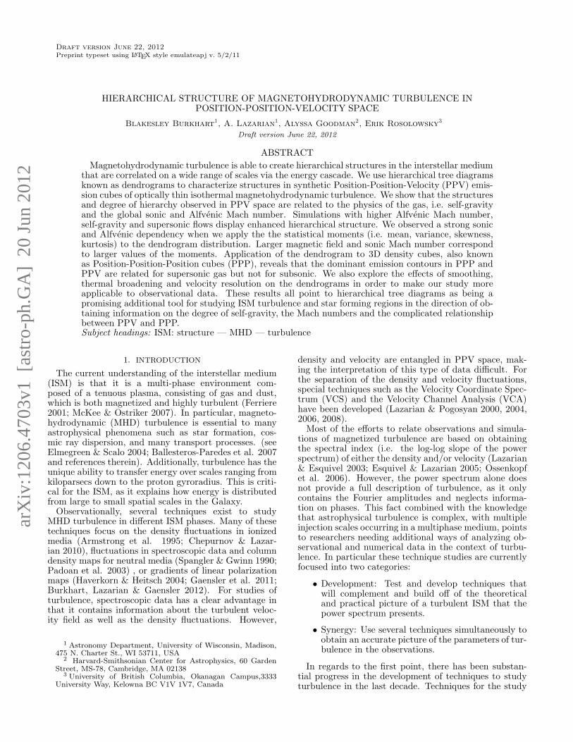
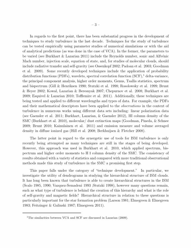
Fig. 1.— The dendrogram for a hypothetical 1D emission profileshowing three local maximum (leaves) and merger points (nodes).The Dendrogram is shown in blue and can be altered by changingthe threshold level δ to higher or lower values. In this example,increasing the value of δ will merge the smallest leaf into the largerstructure. The local maximum (green dots) and merger points (i.e.nodes, red dot) are the values used to create a distribution ξ.

The dendrogram is a tree diagram that can be usedin 1D, 2D or 3D spaces to characterize how and wherelocal maxima merge as a function of a threshold param-eter. Although this paper uses the dendrogram in 3DPPV space to characterize the merger of local maximaof emission, it is more intuitive to understand the 1Dand 2D applications. A 1D example of the dendrogramalgorithm for an emission profile is shown in Figure 1.In this case, the threshold value is called δ, and is theminimum amplitude above a merger point that a localmaximum must be before it is considered distinct. Thatis, if a merger point (or node) is given by n and a localmaximum is given by Lm then in order for a given localmax Lm1 to be considered significant, Lm1 − n1,2 > δ.If Lm1−n1,2 ≤ δ. then Lm1 would merge into Lm2 andno longer be considered distinct.For 2D data, a common analogy (see Houlahan & Scalo

1992, Rosolowsky et al. 2008) is to think of the dendro-gram technique as a descriptor of an underwater moun-tain chain. As the water level is lowered, first one wouldsee the peaks of the mountain, then mountain valleys(saddle points) and as more water is drained, the peaksmay merge together into larger objects. The dendrogramstores information about the peaks and merger levels ofthe mountain chain.The dendrogram is similar to many other statistics that

employ a user defined threshold value in order to clas-sify structure. By varying the threshold parameter δ(see Figure 1), different dendrogram local max distribu-tions are created. An example of another statistic thatutilizes a density/emission threshold value is the Genusstatistic, which has proven useful for studying ISM topol-ogy (Lazarian, Pogosyan& Esquivel 2002; Lazarian 2004;Kim & Park 2007; Kowal et al. 2007; Chepurnov et al.2008). For the Genus technique, the variation of thethreshold value is a critical point in understanding the

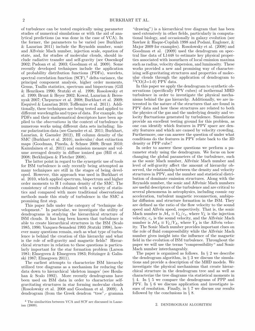
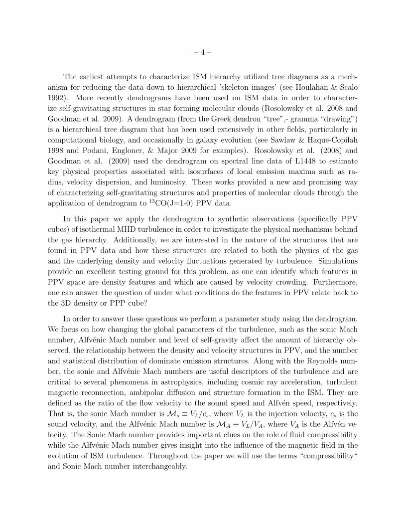
Fig. 2.— List of the simulations and their properties. We usedifferent colors to differentiate the parameter space. We define thesubsonic regimes as anything less then Ms=1 and the supersonicregime as Ms > 1. Two Alfvenic regimes exist for each sonic Machnumber: super-Alfvenic and sub-Alfvenic.

topology of the data in question.For our purposes, we examine the dendrogram in 3D

PPV space (see Rosolowsky et al. 2008; Goodman et al.2009 for more information on the dendrogram algorithmapplied in PPV). In the 3D case, it is useful to thinkof each point in the dendrogram as representing a 3Dcontour (isosurface) in the data cube at a given level. Asδ sets the definition for “local maximum,” setting it toohigh will produce a dendrogram that may miss importantsubstructures while setting it very low may produce adendrogram that is dominated by noise. While δ setsthe value for the minimum leaf length, the branches ofthe tree do not directly depend on δ, and only depend onat what intensity level a set of local maximum are joinedat.The issues of noise and the dendrogram were discussed

extensively in Rosolowsky et al. 2008. While the den-drogram is designed to present only the essential featuresof the data, noise will mask the low-amplitude or highspatial frequency variation in the emission structures. Inextreme cases where the threshold value is not set highenough or the signal-to-noise is very low, noise can resultin local maxima that do not correspond to real structure.As a result, the algorithm has a built in noise suppres-sion criteria which only recognizes structures that have 4σrms significance above δ. Such a criterion has been pre-viously used in data cube analysis as noise fluctuationswill typically produce 1 σrms variations ( Brunt et al.2003; Rosolowsky & Blitz 2005; Rosolowsky et al. 2008).Once the dendrogram is created, there are multiple

ways of viewing the information it provides such as:

• A tree diagram (the dendrogram itself).

• 3D viewing of the isocontours and their connectiv-ity in PPV space.

• A histogram of the dendrogram leaf and node val-ues (i.e. intensities), which can then be further

4 BURKHART ET AL.

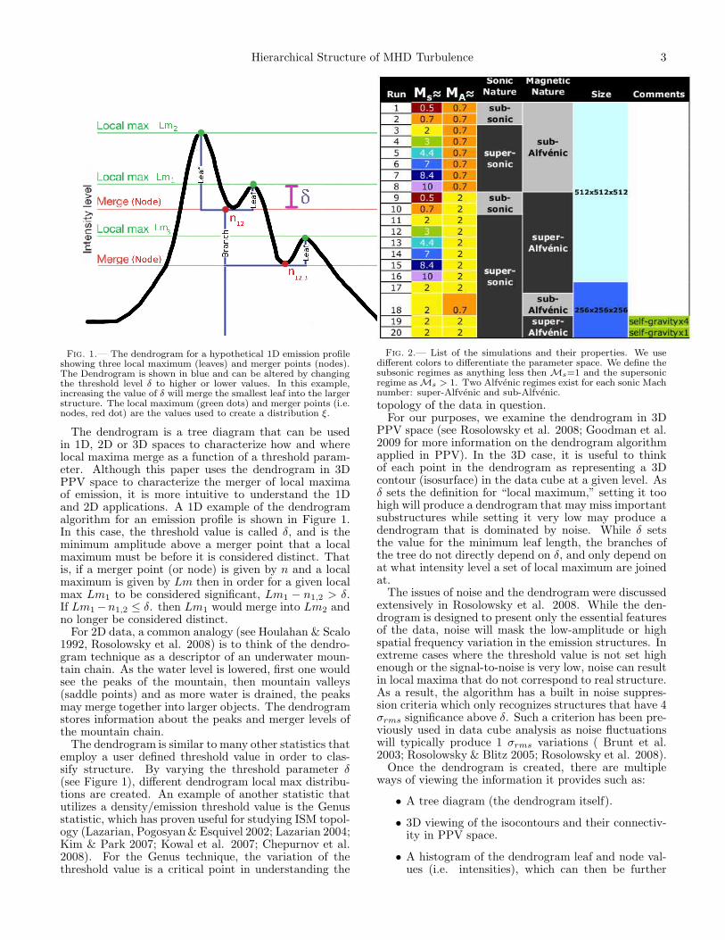
Fig. 3.— Different ways of viewing dendrogram information used in this paper. Here we show an example for supersonic sub-Alfvenicturbulence (model 3 from Figure 2) for threshold values δ=14,16,20 (left, center, right columns). The top row represents the isosurfaces inthe PPV data and the middle row is the corresponding dendrogram (the black line is a reference marker for δ) with colors matching to theisosurface structures. Note there is no information on the x-axis of the tree diagram as the branches are sorted not to cross. However thisstill preserves all information about connectivity and hierarchy at the expense of positional information. The bottom row is the histogramof the resulting tree diagram, including the leaves, branches and nodes. The red line is a reference marker at intensity level 25. The units ofintensity on the y-axis of the tree diagrams in the middle row could be in brightness temperature (Tb) for scaled simulations or observations.

statistically analyzed.

We note that this third point is a novel interpretationof the dendrogram that we develop in this work. Here thehistogram will be composed of intensity values importantto the hierarchical structure of the image. This includesthe leaves, denoted by Lm, and nodes, denoted with n.In this case we define a distribution:

ξ=

(

Lm1 Lm2 Lm3 Lm4....Lmn

n1,2 n3,4 n(1,2),(3,4) ...nm,n

)

This interpretation is visualized in Figure 3 and furtherdescribed below. To produce the dendrogram, we firstidentify a population of local maxima as the points whichare larger than all surrounding voxels touching along theface (not along edges or corners). This large set of lo-cal maxima is then reduced by examining each maximumand searching for the smallest contour level that containsonly that maximum. If this contour level is less than δ be-low the local maximum, that local maximum is removedfrom consideration in the leaf population (this differencein data values is the vertical length of the “leaves” of thedendrogram).Once the leaves (local maxima) of the dendrogram are

established, we contour the data with a large numberof levels (500 specifically, see Rosolowsky et al. 2008;Goodman et al. 2009). The dendrogram “branches” aregraphically constructed by connecting the various sets

of maxima at the contour levels where they are joined(see Figure 1 for a 1D example). For graphical presen-tation, the leaves of the structure tree are shuffled untilthe branches do not cross when plotting. As a result, thex-axis of the dendrogram contains no information. Moreinformation on the dendrogram algorithm can be foundin Goodman et al. (2009) in the Supplementary Methodssection and in Rosolowsky et al. (2008).The purpose of this paper is to use dendrogram to char-

acterize the observed hierarchy seen in the data. Weare not necessarily interested in individual clumps foundin the synthetic PPV data, but rather characterizinghow the structures and hierarchy found in simulations ofMHD turbulence depend on parameters such as the levelof turbulence, magnetic fields, and self-gravity. Whileturbulence has often been cited as the cause of the ob-served hierarchical structure in the ISM (Stutzki 1998),it is unclear to what extent magnetic fields, gas pressure,and gravity play roles in the creation of ISM hierarchyeven though these parameters are known to drasticallychange the PDF and spectrum of both column densityand PPV data (see Falgarone 1994; Kowal et al. 2007;Tofflemire et al. 2011).

3. DATA

We generate a database of twenty 3D numerical simu-lations of isothermal compressible (MHD) turbulence by

Hierarchical Structure of MHD Turbulence 5

0.0 0.5 1.0 1.5Log δ

1.5

2.0

2.5

3.0

3.5

4.0Lo

g N

-3.9

-2.2

-1.1

0.5 1.0 1.5 2.0Log δ

-4.1 -3.3

-1.67

Ms=0.7Ms=3.0Ms=8.0

MA=0.7 MA=2.0

3 4 5 6 7 8δ

200

400

600

800

1000

Num

ber

of S

egm

ents

Ms=0.5Ms=3.0Ms=8.0Ms=10

3 4 5 6 7 8δ

MA=2.0MA=0.7

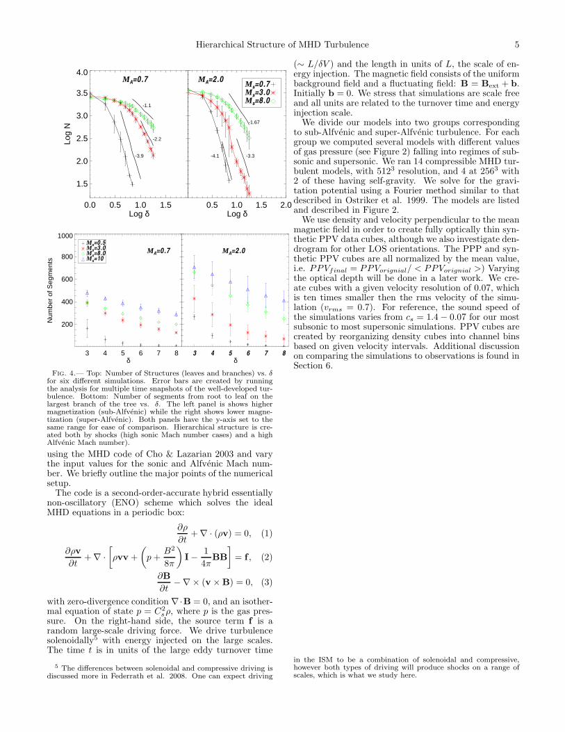
Fig. 4.— Top: Number of Structures (leaves and branches) vs. δfor six different simulations. Error bars are created by runningthe analysis for multiple time snapshots of the well-developed tur-bulence. Bottom: Number of segments from root to leaf on thelargest branch of the tree vs. δ. The left panel is shows highermagnetization (sub-Alfvenic) while the right shows lower magne-tization (super-Alfvenic). Both panels have the y-axis set to thesame range for ease of comparison. Hierarchical structure is cre-ated both by shocks (high sonic Mach number cases) and a highAlfvenic Mach number).

using the MHD code of Cho & Lazarian 2003 and varythe input values for the sonic and Alfvenic Mach num-ber. We briefly outline the major points of the numericalsetup.The code is a second-order-accurate hybrid essentially

non-oscillatory (ENO) scheme which solves the idealMHD equations in a periodic box:

∂ρ

∂t+∇ · (ρv) = 0, (1)

∂ρv

∂t+∇ ·

[

ρvv +

(

p+B2

8π

)

I−1

4πBB

]

= f , (2)

∂B

∂t−∇× (v ×B) = 0, (3)

with zero-divergence condition ∇·B = 0, and an isother-mal equation of state p = C2

sρ, where p is the gas pres-sure. On the right-hand side, the source term f is arandom large-scale driving force. We drive turbulencesolenoidally5 with energy injected on the large scales.The time t is in units of the large eddy turnover time

5 The differences between solenoidal and compressive driving isdiscussed more in Federrath et al. 2008. One can expect driving

(∼ L/δV ) and the length in units of L, the scale of en-ergy injection. The magnetic field consists of the uniformbackground field and a fluctuating field: B = Bext + b.Initially b = 0. We stress that simulations are scale freeand all units are related to the turnover time and energyinjection scale.We divide our models into two groups corresponding

to sub-Alfvenic and super-Alfvenic turbulence. For eachgroup we computed several models with different valuesof gas pressure (see Figure 2) falling into regimes of sub-sonic and supersonic. We ran 14 compressible MHD tur-bulent models, with 5123 resolution, and 4 at 2563 with2 of these having self-gravity. We solve for the gravi-tation potential using a Fourier method similar to thatdescribed in Ostriker et al. 1999. The models are listedand described in Figure 2.We use density and velocity perpendicular to the mean

magnetic field in order to create fully optically thin syn-thetic PPV data cubes, although we also investigate den-drogram for other LOS orientations. The PPP and syn-thetic PPV cubes are all normalized by the mean value,i.e. PPVfinal = PPVorignial/ < PPVorignial >) Varyingthe optical depth will be done in a later work. We cre-ate cubes with a given velocity resolution of 0.07, whichis ten times smaller then the rms velocity of the simu-lation (vrms = 0.7). For reference, the sound speed ofthe simulations varies from cs = 1.4− 0.07 for our mostsubsonic to most supersonic simulations. PPV cubes arecreated by reorganizing density cubes into channel binsbased on given velocity intervals. Additional discussionon comparing the simulations to observations is found inSection 6.

in the ISM to be a combination of solenoidal and compressive,however both types of driving will produce shocks on a range ofscales, which is what we study here.

6 BURKHART ET AL.

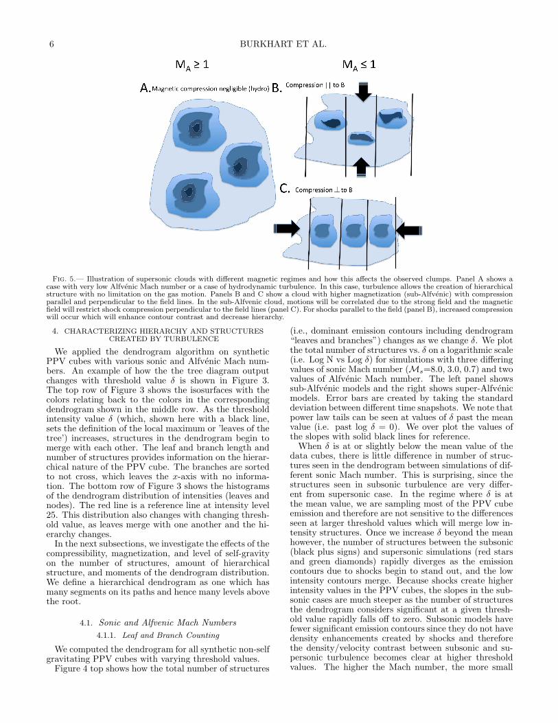
Fig. 5.— Illustration of supersonic clouds with different magnetic regimes and how this affects the observed clumps. Panel A shows acase with very low Alfvenic Mach number or a case of hydrodynamic turbulence. In this case, turbulence allows the creation of hierarchicalstructure with no limitation on the gas motion. Panels B and C show a cloud with higher magnetization (sub-Alfvenic) with compressionparallel and perpendicular to the field lines. In the sub-Alfvenic cloud, motions will be correlated due to the strong field and the magneticfield will restrict shock compression perpendicular to the field lines (panel C). For shocks parallel to the field (panel B), increased compressionwill occur which will enhance contour contrast and decrease hierarchy.

4. CHARACTERIZING HIERARCHY AND STRUCTURESCREATED BY TURBULENCE

We applied the dendrogram algorithm on syntheticPPV cubes with various sonic and Alfvenic Mach num-bers. An example of how the the tree diagram outputchanges with threshold value δ is shown in Figure 3.The top row of Figure 3 shows the isosurfaces with thecolors relating back to the colors in the correspondingdendrogram shown in the middle row. As the thresholdintensity value δ (which, shown here with a black line,sets the definition of the local maximum or ’leaves of thetree’) increases, structures in the dendrogram begin tomerge with each other. The leaf and branch length andnumber of structures provides information on the hierar-chical nature of the PPV cube. The branches are sortedto not cross, which leaves the x-axis with no informa-tion. The bottom row of Figure 3 shows the histogramsof the dendrogram distribution of intensities (leaves andnodes). The red line is a reference line at intensity level25. This distribution also changes with changing thresh-old value, as leaves merge with one another and the hi-erarchy changes.In the next subsections, we investigate the effects of the

compressibility, magnetization, and level of self-gravityon the number of structures, amount of hierarchicalstructure, and moments of the dendrogram distribution.We define a hierarchical dendrogram as one which hasmany segments on its paths and hence many levels abovethe root.

4.1. Sonic and Alfvenic Mach Numbers

4.1.1. Leaf and Branch Counting

We computed the dendrogram for all synthetic non-selfgravitating PPV cubes with varying threshold values.Figure 4 top shows how the total number of structures

(i.e., dominant emission contours including dendrogram“leaves and branches”) changes as we change δ. We plotthe total number of structures vs. δ on a logarithmic scale(i.e. Log N vs Log δ) for simulations with three differingvalues of sonic Mach number (Ms=8.0, 3.0, 0.7) and twovalues of Alfvenic Mach number. The left panel showssub-Alfvenic models and the right shows super-Alfvenicmodels. Error bars are created by taking the standarddeviation between different time snapshots. We note thatpower law tails can be seen at values of δ past the meanvalue (i.e. past log δ = 0). We over plot the values ofthe slopes with solid black lines for reference.When δ is at or slightly below the mean value of the

data cubes, there is little difference in number of struc-tures seen in the dendrogram between simulations of dif-ferent sonic Mach number. This is surprising, since thestructures seen in subsonic turbulence are very differ-ent from supersonic case. In the regime where δ is atthe mean value, we are sampling most of the PPV cubeemission and therefore are not sensitive to the differencesseen at larger threshold values which will merge low in-tensity structures. Once we increase δ beyond the meanhowever, the number of structures between the subsonic(black plus signs) and supersonic simulations (red starsand green diamonds) rapidly diverges as the emissioncontours due to shocks begin to stand out, and the lowintensity contours merge. Because shocks create higherintensity values in the PPV cubes, the slopes in the sub-sonic cases are much steeper as the number of structuresthe dendrogram considers significant at a given thresh-old value rapidly falls off to zero. Subsonic models havefewer significant emission contours since they do not havedensity enhancements created by shocks and thereforethe density/velocity contrast between subsonic and su-personic turbulence becomes clear at higher thresholdvalues. The higher the Mach number, the more small

Hierarchical Structure of MHD Turbulence 7

scale enhancements we expect to see.As δ increases, differences between supersonic (Ms=

3.0) and very supersonic (Ms= 8.0) cases become moreapparent, as the slopes for the Ms= 3.0 case are steeper.This is because interacting shocks in the Ms= 8.0 aremuch stronger, and hence there is more contrast in theemission contours. Thus, as we increase δ, the structuresmerge more rapidly for lower values of the sonic Machnumber.Comparison between the left and right panels shows

that the magnetic field also affects the number of struc-tures and the trend with the threshold value. Whenδ is low (i.e. there is more structure in the tree) thelow magnetized case (super-Alfvenic, right panel) showsslightly more structures then the highly magnetized case.However, as the threshold value increases, the numberof structures decreases more rapidly in the case of thesuper-Alfvenic case, which is evident in that the slopesare steeper regardless of the sonic Mach number. Thesetrends with magnetic field are due to differences betweenMHD and hydrodynamic turbulence. For super-Alfvenicgas (which is close to hydrodynamic), turbulent eddiescan evolve with a full 3D range of motion and have moredegrees of freedom then plasma turbulence in the pres-ence of a strong magnetic field. For turbulence in thesub-Alfvenic regime, the strong field creates anisotropyin the eddies, which are stretched along the directionof the mean field line. This limits the range of motionof the eddies which in turn, limits their ability to inter-act. Structures in the supersonic sub-Alfvenic cases showmore contrast in PPV, meaning that the local maximumare generally higher and differences from the mean aremore pronounced (this will be discussed more in the nextsubsection with the moments). Hence, as we increase δ,the structures in sub-Alfvenic turbulence do not mergewith each other as quickly as in the case of the super-Alfvenic turbulence, which has less contrast in its emis-sion cubes.In light of this, we might also expect the structures in

sub-Alfvenic turbulence to show less hierarchical struc-ture overall. A test of hierarchy is to count the number ofsegments along the largest branch, from leaf to root. Thebottom plot of Figure 4 shows the number of segmentsfrom root to leaf on the largest branch vs. the thresh-old parameter δ. Similar to what was shown in the topfigure, the sonic Mach number has a strong relation tothe amount of hierarchical structure created in the gas.Higher sonic Mach number yields more shocks which inturn produce more high density clumps and more hier-archical structures in PPV space. However, as expectedfrom the top plot, the magnetic field seems to also playa strong role in the hierarchical branching. Comparisonbetween the y-axis values of the left and right plots re-veals that a larger Alfvenic Mach number creates morehierarchical structure in the PPV dendrogram. In thecase of super-Alfvenic turbulence, magnetization is lowand hence the structures created are closer to that ofhydrodynamic turbulence, which is well known to showfractal behavior and hierarchical eddies. As turbulencetransitions to sub-Alfvenic, it become magnetically dom-inated with fewer degrees of freedom. The contrast insub-Alfvenic PPV data is higher, and hence there is lesshierarchical structure as compared with super-Alfvenicturbulence.

We illustrate these findings in Figure 5. Case A showsa cloud with a global Alfvenic Mach number ≥ 1 whilecases B and C show the same cloud with global AlfvenicMach number ≤ 1 but with compression parallel and per-pendicular to the field. All cases are assumed to have thesame supersonic value of the sonic Mach number. Case Ashows hierarchical structure forming in clumps that arenot affected strongly by the magnetic field. The clump-ing and hierarchy is due to compression via shocks andthe shredding effect of hydrodynamic turbulence. Forcase B and C, we now consider how this picture changesif we introduce a strong magnetic field. For shock com-pression parallel to the field lines (Case B), the clumpswill be confined in the direction perpendicular to thefield, and thus the compression will squeeze the clumps,decrease the hierarchy in the gas, create additional largedensity contrast. For shock compression perpendicularto the field lines, in this case the magnetic pressure rel-ative to the shock compression is much higher, and theclumps will not feel as much of the compression. Thusin case B and C, the contrast is higher while hierarchicalstructure is less.These results have interesting implications for hierar-

chical structures in interstellar and star forming clouds,which we will discuss more in the discussion section (sec-tion 7).The plots in Figure 4 are for PPV cubes with LOS

taken perpendicular to the mean magnetic field. Wetested our results for LOS taken parallel to the meanmagnetic field and found similar results.

4.1.2. Statistics of the Dendrogram Distribution

A dendrogram is a useful representation of PPV datain part because there are multiple ways of exploring theinformation on the data hierarchy. In this section we in-vestigate how the statistical moments of the distributionof the dendrogram tree (see bottom panels of Figure 3 forexample) changes as we change the threshold parameterδ and how these changes depend on the compressibilityand magnetization of turbulence. We consider a distri-bution ξ containing all leaves and merging contour val-ues in a given dendrogram. The question that forms thebasis of our investigation in this section is: Do the mo-ments of the distribution ξ have any dependencies on theconditions of the gas (i.e. the sonic and Alfvenic Machnumber) and how does this relate back to the previoussubsection?The 1st and 2nd order statistical moments (mean

and variance) used here are defined as follows: µξ =1N

∑Ni=1 (ξi) and νξ = 1

N−1

∑Ni=1

(

ξi − ξ)2, respectively.

The standard deviation is related to the variance as:σ2ξ = νξ. The 3rd and 4th order moments (skewness

and kurtosis) are defined as:

γξ =1

N

N∑

i=1

(

ξi − µξ

σξ

)3

(4)

βξ =1

N

N∑

i=1

(

ξi − µξ

σξ

)4

− 3 (5)

We calculate the moments of the dendrogram tree dis-tribution while varying our simulation parameter space.

8 BURKHART ET AL.

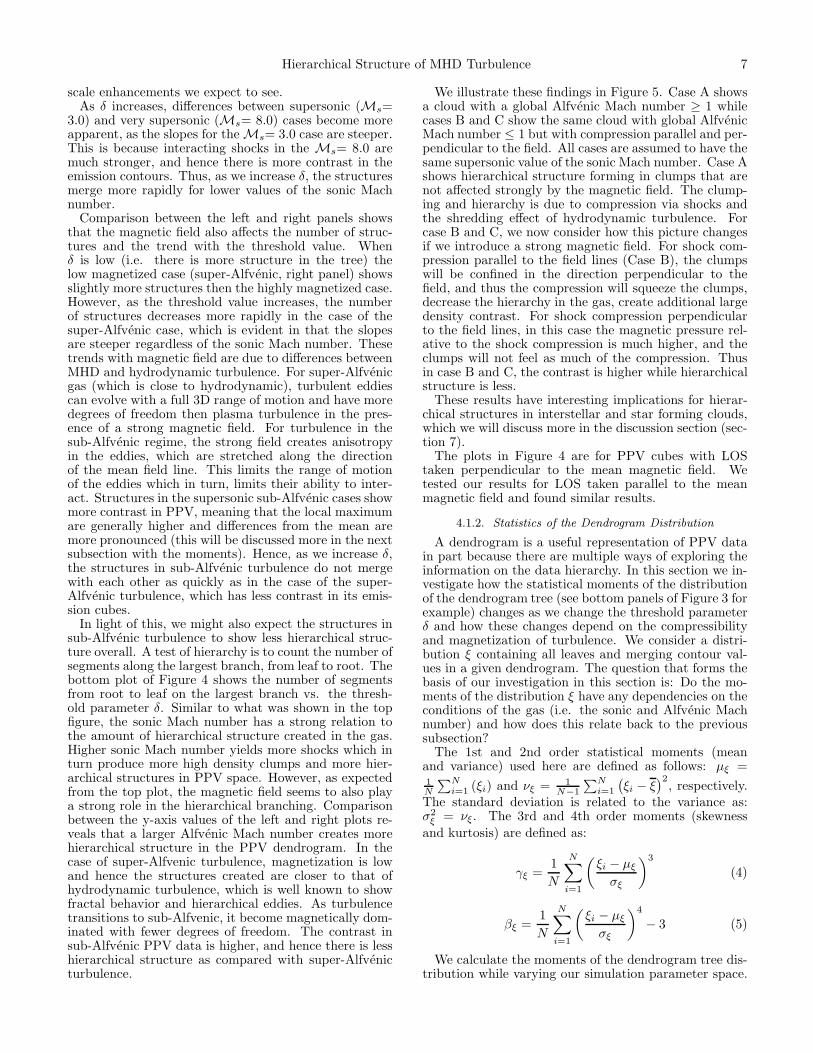
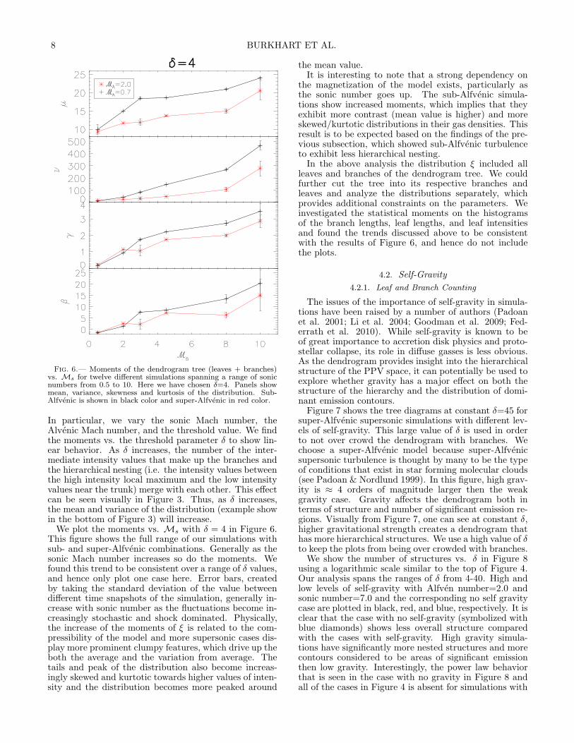
Fig. 6.— Moments of the dendrogram tree (leaves + branches)vs. Ms for twelve different simulations spanning a range of sonicnumbers from 0.5 to 10. Here we have chosen δ=4. Panels showmean, variance, skewness and kurtosis of the distribution. Sub-Alfvenic is shown in black color and super-Alfvenic in red color.

In particular, we vary the sonic Mach number, theAlvenic Mach number, and the threshold value. We findthe moments vs. the threshold parameter δ to show lin-ear behavior. As δ increases, the number of the inter-mediate intensity values that make up the branches andthe hierarchical nesting (i.e. the intensity values betweenthe high intensity local maximum and the low intensityvalues near the trunk) merge with each other. This effectcan be seen visually in Figure 3. Thus, as δ increases,the mean and variance of the distribution (example showin the bottom of Figure 3) will increase.We plot the moments vs. Ms with δ = 4 in Figure 6.

This figure shows the full range of our simulations withsub- and super-Alfvenic combinations. Generally as thesonic Mach number increases so do the moments. Wefound this trend to be consistent over a range of δ values,and hence only plot one case here. Error bars, createdby taking the standard deviation of the value betweendifferent time snapshots of the simulation, generally in-crease with sonic number as the fluctuations become in-creasingly stochastic and shock dominated. Physically,the increase of the moments of ξ is related to the com-pressibility of the model and more supersonic cases dis-play more prominent clumpy features, which drive up theboth the average and the variation from average. Thetails and peak of the distribution also become increas-ingly skewed and kurtotic towards higher values of inten-sity and the distribution becomes more peaked around

the mean value.It is interesting to note that a strong dependency on

the magnetization of the model exists, particularly asthe sonic number goes up. The sub-Alfvenic simula-tions show increased moments, which implies that theyexhibit more contrast (mean value is higher) and moreskewed/kurtotic distributions in their gas densities. Thisresult is to be expected based on the findings of the pre-vious subsection, which showed sub-Alfvenic turbulenceto exhibit less hierarchical nesting.In the above analysis the distribution ξ included all

leaves and branches of the dendrogram tree. We couldfurther cut the tree into its respective branches andleaves and analyze the distributions separately, whichprovides additional constraints on the parameters. Weinvestigated the statistical moments on the histogramsof the branch lengths, leaf lengths, and leaf intensitiesand found the trends discussed above to be consistentwith the results of Figure 6, and hence do not includethe plots.

4.2. Self-Gravity

4.2.1. Leaf and Branch Counting

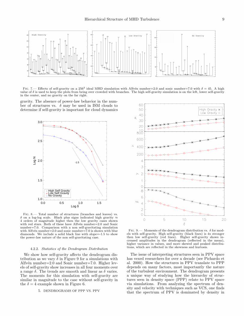
The issues of the importance of self-gravity in simula-tions have been raised by a number of authors (Padoanet al. 2001; Li et al. 2004; Goodman et al. 2009; Fed-errath et al. 2010). While self-gravity is known to beof great importance to accretion disk physics and proto-stellar collapse, its role in diffuse gasses is less obvious.As the dendrogram provides insight into the hierarchicalstructure of the PPV space, it can potentially be used toexplore whether gravity has a major effect on both thestructure of the hierarchy and the distribution of domi-nant emission contours.Figure 7 shows the tree diagrams at constant δ=45 for

super-Alfvenic supersonic simulations with different lev-els of self-gravity. This large value of δ is used in orderto not over crowd the dendrogram with branches. Wechoose a super-Alfvenic model because super-Alfvenicsupersonic turbulence is thought by many to be the typeof conditions that exist in star forming molecular clouds(see Padoan & Nordlund 1999). In this figure, high grav-ity is ≈ 4 orders of magnitude larger then the weakgravity case. Gravity affects the dendrogram both interms of structure and number of significant emission re-gions. Visually from Figure 7, one can see at constant δ,higher gravitational strength creates a dendrogram thathas more hierarchical structures. We use a high value of δto keep the plots from being over crowded with branches.We show the number of structures vs. δ in Figure 8

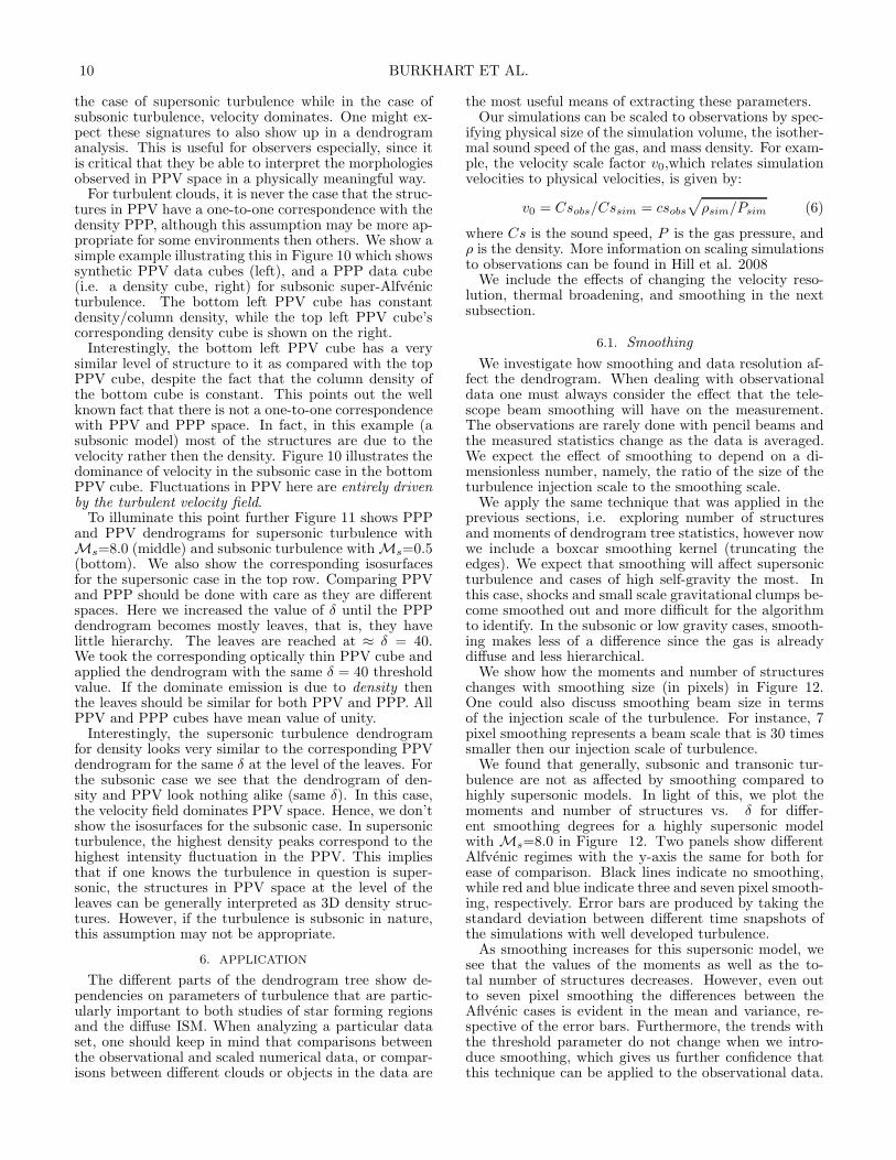
using a logarithmic scale similar to the top of Figure 4.Our analysis spans the ranges of δ from 4-40. High andlow levels of self-gravity with Alfven number=2.0 andsonic number=7.0 and the corresponding no self gravitycase are plotted in black, red, and blue, respectively. It isclear that the case with no self-gravity (symbolized withblue diamonds) shows less overall structure comparedwith the cases with self-gravity. High gravity simula-tions have significantly more nested structures and morecontours considered to be areas of significant emissionthen low gravity. Interestingly, the power law behaviorthat is seen in the case with no gravity in Figure 8 andall of the cases in Figure 4 is absent for simulations with

Hierarchical Structure of MHD Turbulence 9

Fig. 7.— Effects of self-gravity on a 2563 ideal MHD simulation with Alfven number=2.0 and sonic number=7.0 with δ = 45. A highvalue of δ is used to keep the plots from being over crowded with branches. The high self-gravity simulation is on the left, lower self-gravityin the center, and no gravity on the far right.

gravity. The absence of power-law behavior in the num-ber of structures vs. δ may be used in ISM clouds todetermine if self-gravity is important for cloud dynamics

0.0 0.5 1.0 1.5Log δ

1.0

1.5

2.0

2.5

3.0

Log

N

No GravityLow Self GravityHigh Self Gravity

-1.5

Fig. 8.— Total number of structures (branches and leaves) vs.δ on a log-log scale. Black plus signs indicated high gravity ≈

4 orders of magnitude higher then the low gravity cases shownwith red stars. Both of these have Alfven number=2.0 and Sonicnumber=7.0. Comparison with a non self-gravitating simulationwith Alfven number=2.0 and sonic number=7.0 is shown with bluediamonds. We include a solid black line with slope=-1.5 to showthe power-law nature of the non self-gravitating case.

4.2.2. Statistics of the Dendrogram Distribution

We show how self-gravity affects the dendrogram dis-tribution as we vary δ in Figure 9 for a simulations withAlfven number=2.0 and Sonic number=7.0. Higher lev-els of self-gravity show increases in all four moments overa range δ. The trends are smooth and linear as δ varies.The moments for this simulation with self-gravity aresimilar in magnitude to the case without self-gravity inthe δ = 4 example shown in Figure 6.

5. DENDROGRAMS OF PPP VS. PPV

Fig. 9.— Moments of the dendrogram distribution vs. δ for mod-els with self-gravity. High self-gravity (black lines) is 4x strongerthen low self-gravity (red lines). Higher self-gravity shows in-creased amplitudes in the dendrogram (reflected in the mean),higher variance in values, and more skewed and peaked distribu-tions, which are reflected in the skewness and kurtosis.

The issue of interpreting structures seen in PPV spacehas vexed researchers for over a decade (see Pichardo etal. 2000). How the structures in PPV translate to PPPdepends on many factors, most importantly the natureof the turbulent environment. The dendrogram presentsa unique way of studying how the hierarchy of struc-tures seen in density space (PPP) relate to PPV spacevia simulations. From analyzing the spectrum of den-sity and velocity with techniques such as VCS, one findsthat the spectrum of PPV is dominated by density in

10 BURKHART ET AL.

the case of supersonic turbulence while in the case ofsubsonic turbulence, velocity dominates. One might ex-pect these signatures to also show up in a dendrogramanalysis. This is useful for observers especially, since itis critical that they be able to interpret the morphologiesobserved in PPV space in a physically meaningful way.For turbulent clouds, it is never the case that the struc-

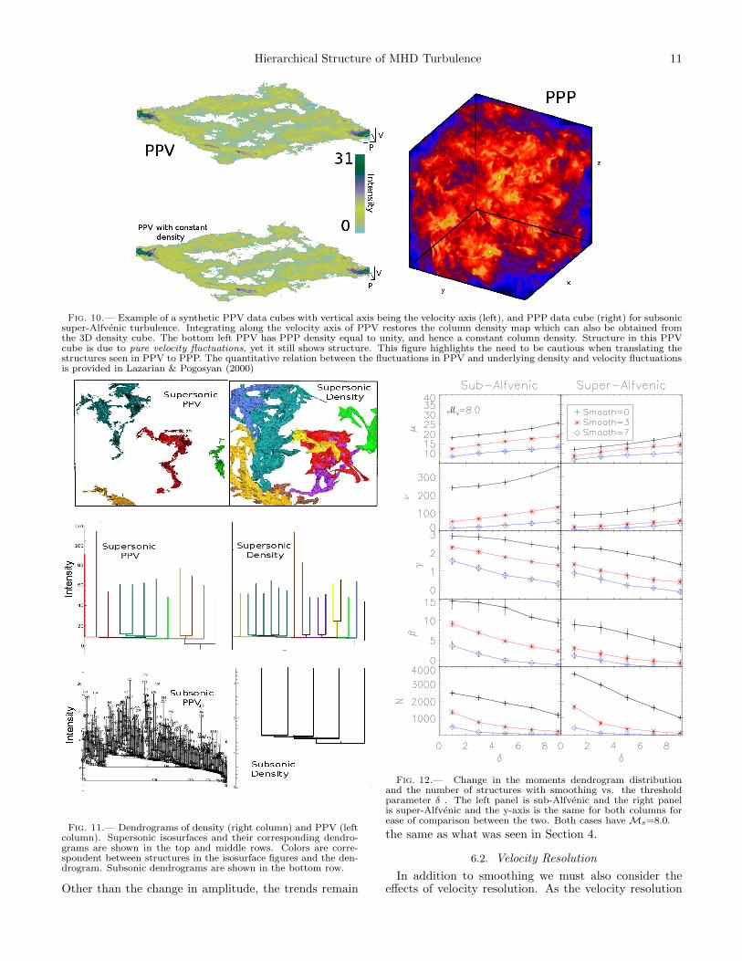
tures in PPV have a one-to-one correspondence with thedensity PPP, although this assumption may be more ap-propriate for some environments then others. We show asimple example illustrating this in Figure 10 which showssynthetic PPV data cubes (left), and a PPP data cube(i.e. a density cube, right) for subsonic super-Alfvenicturbulence. The bottom left PPV cube has constantdensity/column density, while the top left PPV cube’scorresponding density cube is shown on the right.Interestingly, the bottom left PPV cube has a very

similar level of structure to it as compared with the topPPV cube, despite the fact that the column density ofthe bottom cube is constant. This points out the wellknown fact that there is not a one-to-one correspondencewith PPV and PPP space. In fact, in this example (asubsonic model) most of the structures are due to thevelocity rather then the density. Figure 10 illustrates thedominance of velocity in the subsonic case in the bottomPPV cube. Fluctuations in PPV here are entirely drivenby the turbulent velocity field.To illuminate this point further Figure 11 shows PPP

and PPV dendrograms for supersonic turbulence withMs=8.0 (middle) and subsonic turbulence with Ms=0.5(bottom). We also show the corresponding isosurfacesfor the supersonic case in the top row. Comparing PPVand PPP should be done with care as they are differentspaces. Here we increased the value of δ until the PPPdendrogram becomes mostly leaves, that is, they havelittle hierarchy. The leaves are reached at ≈ δ = 40.We took the corresponding optically thin PPV cube andapplied the dendrogram with the same δ = 40 thresholdvalue. If the dominate emission is due to density thenthe leaves should be similar for both PPV and PPP. AllPPV and PPP cubes have mean value of unity.Interestingly, the supersonic turbulence dendrogram

for density looks very similar to the corresponding PPVdendrogram for the same δ at the level of the leaves. Forthe subsonic case we see that the dendrogram of den-sity and PPV look nothing alike (same δ). In this case,the velocity field dominates PPV space. Hence, we don’tshow the isosurfaces for the subsonic case. In supersonicturbulence, the highest density peaks correspond to thehighest intensity fluctuation in the PPV. This impliesthat if one knows the turbulence in question is super-sonic, the structures in PPV space at the level of theleaves can be generally interpreted as 3D density struc-tures. However, if the turbulence is subsonic in nature,this assumption may not be appropriate.

6. APPLICATION

The different parts of the dendrogram tree show de-pendencies on parameters of turbulence that are partic-ularly important to both studies of star forming regionsand the diffuse ISM. When analyzing a particular dataset, one should keep in mind that comparisons betweenthe observational and scaled numerical data, or compar-isons between different clouds or objects in the data are

the most useful means of extracting these parameters.Our simulations can be scaled to observations by spec-

ifying physical size of the simulation volume, the isother-mal sound speed of the gas, and mass density. For exam-ple, the velocity scale factor v0,which relates simulationvelocities to physical velocities, is given by:

v0 = Csobs/Cssim = csobs√

ρsim/Psim (6)

where Cs is the sound speed, P is the gas pressure, andρ is the density. More information on scaling simulationsto observations can be found in Hill et al. 2008We include the effects of changing the velocity reso-

lution, thermal broadening, and smoothing in the nextsubsection.

6.1. Smoothing

We investigate how smoothing and data resolution af-fect the dendrogram. When dealing with observationaldata one must always consider the effect that the tele-scope beam smoothing will have on the measurement.The observations are rarely done with pencil beams andthe measured statistics change as the data is averaged.We expect the effect of smoothing to depend on a di-mensionless number, namely, the ratio of the size of theturbulence injection scale to the smoothing scale.We apply the same technique that was applied in the

previous sections, i.e. exploring number of structuresand moments of dendrogram tree statistics, however nowwe include a boxcar smoothing kernel (truncating theedges). We expect that smoothing will affect supersonicturbulence and cases of high self-gravity the most. Inthis case, shocks and small scale gravitational clumps be-come smoothed out and more difficult for the algorithmto identify. In the subsonic or low gravity cases, smooth-ing makes less of a difference since the gas is alreadydiffuse and less hierarchical.We show how the moments and number of structures

changes with smoothing size (in pixels) in Figure 12.One could also discuss smoothing beam size in termsof the injection scale of the turbulence. For instance, 7pixel smoothing represents a beam scale that is 30 timessmaller then our injection scale of turbulence.We found that generally, subsonic and transonic tur-

bulence are not as affected by smoothing compared tohighly supersonic models. In light of this, we plot themoments and number of structures vs. δ for differ-ent smoothing degrees for a highly supersonic modelwith Ms=8.0 in Figure 12. Two panels show differentAlfvenic regimes with the y-axis the same for both forease of comparison. Black lines indicate no smoothing,while red and blue indicate three and seven pixel smooth-ing, respectively. Error bars are produced by taking thestandard deviation between different time snapshots ofthe simulations with well developed turbulence.As smoothing increases for this supersonic model, we

see that the values of the moments as well as the to-tal number of structures decreases. However, even outto seven pixel smoothing the differences between theAflvenic cases is evident in the mean and variance, re-spective of the error bars. Furthermore, the trends withthe threshold parameter do not change when we intro-duce smoothing, which gives us further confidence thatthis technique can be applied to the observational data.

Hierarchical Structure of MHD Turbulence 11

Fig. 10.— Example of a synthetic PPV data cubes with vertical axis being the velocity axis (left), and PPP data cube (right) for subsonicsuper-Alfvenic turbulence. Integrating along the velocity axis of PPV restores the column density map which can also be obtained fromthe 3D density cube. The bottom left PPV has PPP density equal to unity, and hence a constant column density. Structure in this PPVcube is due to pure velocity fluctuations, yet it still shows structure. This figure highlights the need to be cautious when translating thestructures seen in PPV to PPP. The quantitative relation between the fluctuations in PPV and underlying density and velocity fluctuationsis provided in Lazarian & Pogosyan (2000)

Fig. 11.— Dendrograms of density (right column) and PPV (leftcolumn). Supersonic isosurfaces and their corresponding dendro-grams are shown in the top and middle rows. Colors are corre-spondent between structures in the isosurface figures and the den-drogram. Subsonic dendrograms are shown in the bottom row.

Other than the change in amplitude, the trends remain

Fig. 12.— Change in the moments dendrogram distributionand the number of structures with smoothing vs. the thresholdparameter δ . The left panel is sub-Alfvenic and the right panelis super-Alfvenic and the y-axis is the same for both columns forease of comparison between the two. Both cases have Ms=8.0.

the same as what was seen in Section 4.

6.2. Velocity Resolution

In addition to smoothing we must also consider theeffects of velocity resolution. As the velocity resolution

12 BURKHART ET AL.

changes in PPV space, so do the structures observed. Weinvestigated how the moments of the dendrogram branch+ leaf distribution changed when we vary the velocityresolution. We find that the number of substructuresdrops dramatically as the velocity resolution decreases,from several hundreds to several dozen when changingthe velocity resolution from vres = 0.07 to vres = 0.7.This effect corresponds to the channel sampling droppingfrom≈ 60 down to 15 channels. This may provide too lowa number of statistics in the dendrogram distribution tolook at the moments, however the general trends with thephysical parameters stay consistent with section 4. Thesame holds for the case where we increase the velocityresolution an order of magnitude (up to vres = 0.007).

6.3. Thermal Broadening

The bulk of this paper focuses on the effects of tur-bulence and magnetic fields in the creation of hierarchi-cal structure in ISM clouds, however thermal broaden-ing effects must also be considered as well. Convolutionwith a thermal broadening profile (i.e. a Gaussian) willsmooth out the velocity profiles and generally decreasethe intensities. We convolve the line profiles of eight ofour simulations with sonic Mach numbers ranging fromMs=2.0-10 with Gaussian profiles to mimic the effects ofthermal broadening. The thermal Gaussian has FWHMgiven as the ratio of the turbulent line width to the sonicMach number. As thermal broadening will change the in-tensity range of our simulations, we accordingly changethe values of the threshold parameter δ. We scale δdown from the range used in Section 4 by a factor of< PPVthermal+turbulent > / < PPVturbulent >, in orderto fully sample how the contours merge in the new cubes.We show the effects of including thermal broadening

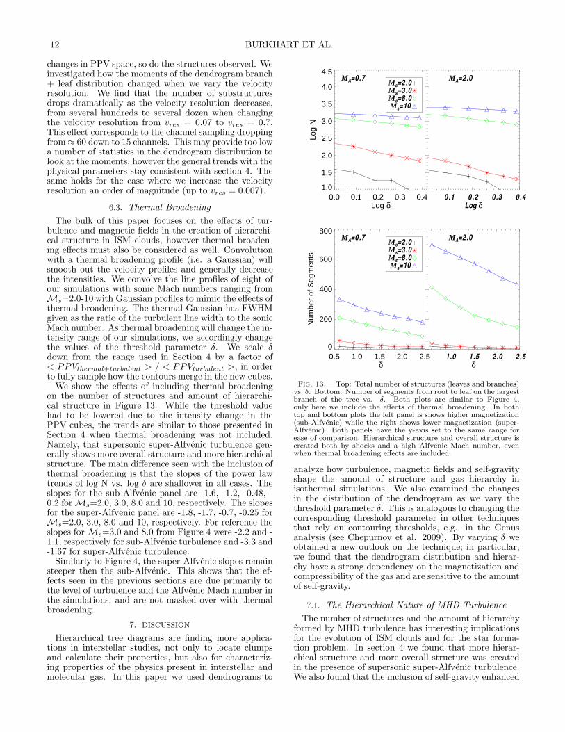
on the number of structures and amount of hierarchi-cal structure in Figure 13. While the threshold valuehad to be lowered due to the intensity change in thePPV cubes, the trends are similar to those presented inSection 4 when thermal broadening was not included.Namely, that supersonic super-Alfvenic turbulence gen-erally shows more overall structure and more hierarchicalstructure. The main difference seen with the inclusion ofthermal broadening is that the slopes of the power lawtrends of log N vs. log δ are shallower in all cases. Theslopes for the sub-Alfvenic panel are -1.6, -1.2, -0.48, -0.2 for Ms=2.0, 3.0, 8.0 and 10, respectively. The slopesfor the super-Alfvenic panel are -1.8, -1.7, -0.7, -0.25 forMs=2.0, 3.0, 8.0 and 10, respectively. For reference theslopes for Ms=3.0 and 8.0 from Figure 4 were -2.2 and -1.1, respectively for sub-Alfvenic turbulence and -3.3 and-1.67 for super-Alfvenic turbulence.Similarly to Figure 4, the super-Alfvenic slopes remain

steeper then the sub-Alfvenic. This shows that the ef-fects seen in the previous sections are due primarily tothe level of turbulence and the Alfvenic Mach number inthe simulations, and are not masked over with thermalbroadening.

7. DISCUSSION

Hierarchical tree diagrams are finding more applica-tions in interstellar studies, not only to locate clumpsand calculate their properties, but also for characteriz-ing properties of the physics present in interstellar andmolecular gas. In this paper we used dendrograms to

0.0 0.1 0.2 0.3 0.4Log δ

1.0

1.5

2.0

2.5

3.0

3.5

4.0

4.5

Log

N

Ms=2.0Ms=3.0Ms=8.0Ms=10

0.1 0.2 0.3 0.4Log δ

MA=0.7 MA=2.0

0.5 1.0 1.5 2.0 2.5δ

0

200

400

600

800

Num

ber

of S

egm

ents

Ms=2.0Ms=3.0Ms=8.0Ms=10

1.0 1.5 2.0 2.5δ

MA=0.7 MA=2.0

Fig. 13.— Top: Total number of structures (leaves and branches)vs. δ. Bottom: Number of segments from root to leaf on the largestbranch of the tree vs. δ. Both plots are similar to Figure 4,only here we include the effects of thermal broadening. In bothtop and bottom plots the left panel is shows higher magnetization(sub-Alfvenic) while the right shows lower magnetization (super-Alfvenic). Both panels have the y-axis set to the same range forease of comparison. Hierarchical structure and overall structure iscreated both by shocks and a high Alfvenic Mach number, evenwhen thermal broadening effects are included.

analyze how turbulence, magnetic fields and self-gravityshape the amount of structure and gas hierarchy inisothermal simulations. We also examined the changesin the distribution of the dendrogram as we vary thethreshold parameter δ. This is analogous to changing thecorresponding threshold parameter in other techniquesthat rely on contouring thresholds, e.g. in the Genusanalysis (see Chepurnov et al. 2009). By varying δ weobtained a new outlook on the technique; in particular,we found that the dendrogram distribution and hierar-chy have a strong dependency on the magnetization andcompressibility of the gas and are sensitive to the amountof self-gravity.

7.1. The Hierarchical Nature of MHD Turbulence

The number of structures and the amount of hierarchyformed by MHD turbulence has interesting implicationsfor the evolution of ISM clouds and for the star forma-tion problem. In section 4 we found that more hierar-chical structure and more overall structure was createdin the presence of supersonic super-Alfvenic turbulence.We also found that the inclusion of self-gravity enhanced

Hierarchical Structure of MHD Turbulence 13

these trends. The relationship between the magnetiza-tion and the cloud dynamics is in the process of beingunderstood, especially in regards to star formation. Starforming clouds are known to be hierarchical in natureand magnetized, but the exact Alfvenic nature is lessclear. The results from this work seem to suggest thatvery hierarchical clouds might tend towards being super-Alfvenic. Several authors have suggested a variety of ev-idence for molecular clouds being super-Alfvenic. Thisincludes the agreement of simulations and observationsof Zeeman-splitting measurements, B vs.ρ relations, MA

vs. ρ relations, statistics of the extinction measurementetc. (Padoan & Nordlund 1999; Lunttila et al. 2008;Burkhart et al. 2009; Crutcher et al. 2009; Collins etal. 2012). Furthermore a study done by Burkhart et al.2009 found that, even in the presence of globally sub-Alfvenic turbulence, the highest density regions tend to-wards being locally super-Alfvenic. This suggests thateven in the case of globally sub-Alfvenic turbulence, thedensest regions might be super-Alfvenic. It is interest-ing that the dendrogram technique also points to super-Alfvenic turbulence as an avenue for hierarchical struc-ture creation. This provides motivation for the dendro-gram technique to be applied to the observational datawith varying threshold value δ in order to see how thenature of the hierarchical structure and total number ofstructures change in the observations.

7.2. Sonic and Alfvenic Mach Numbers from theObservations

In the paper above we provided a systematic study ofthe variations of the dendrogram δ with the sonic andmagnetic Mach numbers. These numbers are critical forunderstanding most of processes in galactic diffuse andmolecular gas, including the process of star formation.Thus, the dendrogram provides an avenue of obtainingthese parameters via comparing observations and simu-lations and/or as a technique for investigating what pro-cesses are creating hierarchical structure in ISM gas.We view this work as the springboard for applying the

technique to the actual data. We claim that for reliablestudies of the interstellar media and molecular clouds it ismost advantageous to combine different techniques. Forinstance, applying the VCA and VCS techniques to PPVdata (see Lazarian 2009 for a review), one can obtain thevelocity and density spectra of turbulence. While thesemeasures are known to depend on Ms and to a lesserdegree on MA (see Beresnyak, Lazarian & Cho 2005,Kowal et al. 2007, Burkhart et al. 2009), the utility ofthe spectra is not in measuring these quantities. Spectraprovide a unique way to investigate how the energy cas-cades between different scales, and shows whether com-paring observations with the simulations with a singlescale of injection is reasonable.The analysis of the anisotropies of correlations using

velocity centroids provides an insight into media mag-netization, i.e., provides MA (Lazarian et al. 2002, Es-quivel & Lazarian 2005), which is complimentary to thetechnique described in this paper. Studies of the skew-ness and kurtosis of the PDFs (see Kowal et al. 2007,Burkhart et al. 2009, 2010) provides measures of thesonic Mach number Ms. Similarly, Tsallis statisticsmeasures (Esquivel & Lazarian 2010, Tofflemire et al.2011) provide additional ways of estimating bothMs and

MA. We feel the approach to obtaining these parame-ters should be conducted with synergetic use of multipletools, such as was done in Burkhart et al. 2010 on theSMC. We feel the dendrogram is a unique tool as it canclassify the hierarchical nature of the data and that itshould be added to a standard set of statistical-tools forstudies of ISM data.All these techniques provide independent ways of eval-

uating parameters of turbulence and therefore their ap-plication to the same data set provides a more reliableestimate of key parameters such as compressibility, mag-netization, and degree of self-gravity. Dendrograms havesome advantages over other statistics designed to searchfor turbulence parameters, in that one can analyze theresulting tree diagram in many different ways, as high-lighted in this paper and in previous works. These in-clude finding local maxima, calculating physical proper-ties of dominate emission, exploring how those clumpsare connected in PPV, varying the threshold and cal-culating moments and level of hierarchy. Of course, oneshould keep in mind that the medium that we investigateobservationally is far from simple. Multiple energy in-jection sources, for example, are not excluded. Thus ob-taining a similar answer with different techniques shouldprovide us with additional confidence in our results.Finally, we should stress, that for studies of astrophys-

ical objects the dendrogram and other statistical mea-sures can be applied locally to different parts of the me-dia. For instance, Burkhart et al. (2010) did not char-acterize the entire SMC with one sonic Mach number.Instead, several measures were applied to parts of theSMC in order to obtain a distribution of the turbulencein the galaxy. A similar local scale selection was appliedalso to the SMC in Chepurnov et al. (2008) using theGenus technique. The same technique should be used toparts of the ISM in the Milky way and may be attemptedfor GMCs. Correlating the variations of the turbulenceproperties with observed properties of the media, e.g.star formation rate should provide insight into how tur-bulence regulates many key astrophysical processes.

8. SUMMARY

We apply dendrograms to isothermal MHD simulationswith varying levels of gravity, compressibility and mag-netization. We find that the dendrogram is a promisingtool for studying both gas connectivity in the ISM as wellas characterizing turbulence. In particular we find that:

• We propose using statistical descriptions of dendro-grams as a means to quantify the degree of hierar-chy present in a PPV data cube.

• Shocks, self-gravity, and super-Alfvenic turbulencecreate the most hierarchical structure in PPVspace.

• The number of dendrogram structures depends pri-marily on the sonic number and the level of self-gravity and secondarily on the global magnetiza-tion.

• The first four statistical moments of the distri-bution of dendrogram leaves and connecting havemonotonic dependencies on the level of self-gravityand the sonic and Alfven Mach numbers over arange of δ.

14 BURKHART ET AL.

• The dendrogram provides a convenient way of com-paring PPP to PPV in simulations. Density struc-tures are dominant in supersonic PPV and not insubsonic. Thus it is more justifiable to comparePPV directly to PPP when the gas is known to besupersonic.

B.B. acknowledges support from the NSF GraduateResearch Fellowship and the NASA Wisconsin SpaceGrant Institution. B.B. is thankful for valuable discus-sions and the use of the Dendrogui code via Chris Beau-mont. A.L. thanks NSF AST 0808118, the Center forMagnetic Self-Organization in Astrophysical and Lab-oratory Plasmas for financial support. This work wascompleted during the stay of A.L. as Alexander-von-Humboldt-Preistrager at the Ruhr-University Bochum.A.G. acknowledges support from NSF Grant No. AST-0908159. E.R. is supported by a Discovery Grant fromNSERC of Canada.

REFERENCES

Armstrong,J. W., Rickett, B. J., Spangler, S. R., 1995, ApJ, 443,209

Ballesteros-Paredes, J., Klessen, R. S., Mac Low, M.-M., &Vazquez-Semadeni, E. 2007, in Protostars and Planets V, ed.B. Reipurth, D. Jewitt, & K. Keil (Tucson, AZ: Univ. ofArizona Press), 63

Beresnyak, A., Lazarian, A., Cho, J., 2005, ApJ, 624, 93Berkhuijsen E., Fletcher, A., 2008, MNRAS, 390, 19Brunt, C. M., Kerton, C. R., & Pomerleau, C., 2003, ApJS, 144,

47Brunt, C., & Heyer, M., 2002, ApJ, 566, 27Brunt, C., 2010, A&A, 513, 67Burkhart, B., Falceta-Goncalves, D., Kowal, G., Lazarian, A.,

2009, ApJ, 693, 250Burkhart, B., Stanimirovic, S., Lazarian, A., Grzegorz, K., 2010,

ApJ, 708, 1204Burkhart, B., Lazarian, A., Gaensler, B., 2012, ApJ, 708, 1204Burkhart, B., & Lazarian, A., 2011, IAUS, 274, 365Chepurnov, A., Gordon, J., Lazarian, A., & Stanimirovic, S.,2008,

ApJ, 688, 1021Chepurnov, A., & Lazarian, A. 2009, ApJ, 693, 1074Chepurnov & Lazarian, 2010, ApJ, 710, 853Cho, J. & Lazarian, A. 2003, MNRAS, 345, 325Collins et al., 2012, ApJ, 750, 13Crutcher, R., Hakobian, N., Troland, T., 2009, ApJ, 692, 844Elmegreen, B. G., & Elmegreen, D. M. 1983, MNRAS, 203, 31Elmegreen, B. G., & Scalo, J. 2004, ARA&A, 42, 211Elmegreen, B. G., 2011, Star Formation in the Local Universe,

Eds. C. Charbonnel & T. Montmerle, EAS Publications SeriesEsquivel, A, & Lazarian, A., 2005, ApJ, 295,479Esquivel, A., & Lazarian, A., 2010, ApJ, 710, 125Falgarone, E., Lis, D. C., Phillips, T. G., Pouquet, A., Porter,

D. H., & Woodward, P. R. 1994, ApJ, 436, 728Ferriere, K., 2001, RvMP, 73, 1031Federrath, C., et al., 2008, ApJ, 688, 79Federrath, C., et al., 2010, ApJ, 713, 269Feitzinger, J. V., & Galinski, T. 1987, A&A, 179, 249Frisch, U., 1995, Turbulence, Univ. of Cambridge PressGaensler et al., 2011, Nature, 478, 214-217Gill, A.G., & Henriksen, R.N., 1990, ApJ, 365, L27Goodman et al., 2009, Nature, 457, 63Goodman, A., Pineda, J., Schnee S., 2009, ApJ, 692, 91Haverkorn, M., & Heitsch, F., 2004, A&A,421, 1011Hill, A. et al., 2008, ApJ, 686, 363Houlahan P., & Scalo J., 1992, ApJ, 393, 172Kang, H., Ryu, D., & Jones, T. W., 2009, ApJ, 695, 1273Kainulainen, J., Beuther, H., Banerjee, R., Federrath, C.,

Henning, T., 2011, A&A, 530, 64Kim, S., Park, G., 2007, ApJ, 663, 244Kowal, G., Lazarian, A. & Beresnyak, A., 2007, ApJ, 658, 423Larson, R.B. 1981, MNRAS, 194, 809

Lazarian, A., 2004, J. Korean Astron. Soc., 37, 563Lazarian, A., 2009, SSR, 143, 357Lazarian A., & Esquivel, A., 2003, ApJ, 592, 37Lazarian, A. & Pogosyan,D., 2000, ApJ, 537, 720Lazarian, A. & Pogosyan, D., 2004, ApJ, 616, 943Lazarian,A. & Pogosyan,D., 2006,ApJ, 652, 1348Lazarian, A. & Pogosyan,D., 2008,ApJ, 686, 350

Lazarian, A., Pogosyan, D., & Esquivel, A. 2002, in ASP Conf.Proc. 276, Seeing Through the Dust: The Detection of H I andthe Exploration of the ISM in Galaxies, ed. A. R. Taylor, T. L.Landecker, & A. G. Willis (San Francisco: ASP), 182

Li, P. S., Normand, M., Mac Low, M., Heitsch, F., 2004, ApJ,605, 800

McKee, C., Ostriker, E., 2007, , ARA&A, 45, 565Ossenkopf, V., & Mac Low, M.-M., 2002, A&A, 390, 307Ossenkopf, V., Esquivel, A., Lazarian, A., & Stutzki, J. 2006,

A&A, 452, 223Ostriker, E., Gammie, C., Stone, J., 1999, ApJ, 513, 259Padoan, P., & Nordlund, A., 1999, ApJ, 526, 27Padoan, P., Rosolowsky, E. W., & Goodman, A. A. 2001, ApJ,

547, 862Padoan, P., Nordlund, A., Rognvaldsson, O. E., & Goodman, A.

A., 2001, in ASP Conf. Ser. 243, From Darkness to Light:Origin and Evolution of Young Stellar Clusters, ed. T.Montmerle, & P. Andre (San Francisco: ASP), 279

Padoan, P., Goodman, A., Juvela, Mika, 2003, ApJ, 588, 881Padoan, P., Juvela, M., Kritsuk, A. G., & Norman, M. L. 2009,

ApJ, 707, L153Pichardo et al. 2000, ApJ, 532, 353Podani, J., Engloner, A., & Major, A., 2009, Stat. Appl. Genet.

Mol. Biol., 22.Price, Federrath, & Brunt, 2011, ApJ, 727Rosolowsky, E., Goodman, A., Wilner, D., Williams, J.,1999,

ApJ, 524, 887Rosolowsky, E., & Blitz, L., 2005, ApJ, 623, 826Rosolowsky, E. W., Pineda, J. E., Kauffmann, J., & Goodman, A.

A. 2008, ApJ, 679, 1338Sawlaw W. & Haque-Copilah, S., 1998, ApJ 509, 595Spangler, S. R., & Gwinn, C. R. 1990, ApJ, 353, L29Toffelmire, B., Burkhart, B., Lazarian, A., 2011, ApJ, 736, 60Scalo, J.S. 1985, in Protostars and Planets II, ed. D.C Black and

M. S. Matthews, (Tucson: Univ. of Arizona Press), p. 201Scalo, J. 1990, in Physical Processes in Fragmentation and Star

Formation, eds. R. Capuzzo-Dolcetta, C. Chiosi, & A. Di Fazio,Dordrecht: Kluwer, p. 151

Stutzki, J., Bensch, F., Heithausen, A., Ossenkopf, V., Zielinsky,M., 1998, A&A, 336,697

Vazquez-Semadeni, E., 1993, ApJ, 423, 681

arX

iv:1

206.

4703

v1 [

astr

o-ph

.GA

] 2

0 Ju

n 20

12

Hierarchical Structure of Magnetohydrodynamic Turbulence In

Position-Position-Velocity Space

Blakesley Burkhart1, A. Lazarian1, Alyssa Goodman2, Erik Rosolowsky3

ABSTRACT

Magnetohydrodynamic turbulence is able to create hierarchical structures in

the interstellar medium that are correlated on a wide range of scales via the en-

ergy cascade. We use hierarchical tree diagrams known as dendrograms to char-

acterize structures in synthetic Position-Position-Velocity (PPV) emission cubes

of optically thin isothermal magnetohydrodynamic turbulence. We show that

the structures and degree of hierarchy observed in PPV space are related to the

physics of the gas, i.e. self-gravity and the global sonic and Alfvenic Mach num-

ber. Simulations with higher Alfvenic Mach number, self-gravity and supersonic

flows display enhanced hierarchical structure. We observed a strong sonic and

Alfvenic dependency when we apply the the statistical moments (i.e. mean, vari-

ance, skewness, kurtosis) to the dendrogram distribution. Larger magnetic field

and sonic Mach number correspond to larger values of the moments. Application

of the dendrogram to 3D density cubes, also known as Position-Position-Position

cubes (PPP), reveals that the dominant emission contours in PPP and PPV are

related for supersonic gas but not for subsonic. We also explore the effects of

smoothing, thermal broadening and velocity resolution on the dendrograms in

order to make our study more applicable to observational data. These results

all point to hierarchical tree diagrams as being a promising additional tool for

studying ISM turbulence and star forming regions in the direction of obtaining

information on the degree of self-gravity, the Mach numbers and the complicated

relationship between PPV and PPP.

Subject headings: ISM: structure — MHD — turbulence

1Astronomy Department, University of Wisconsin, Madison, 475 N. Charter St., WI 53711, USA

2 Harvard-Smithsonian Center for Astrophysics, 60 Garden Street, MS-78, Cambridge, MA 02138

3University of British Columbia, Okanagan Campus,3333 University Way, Kelowna BC V1V 1V7, Canada

– 2 –

1. Introduction

The current understanding of the interstellar medium (ISM) is that it is a multi-phase

environment composed of a tenuous plasma, consisting of gas and dust, which is both mag-

netized and highly turbulent (Ferriere 2001; McKee & Ostriker 2007). In particular, mag-

netohydrodynamic (MHD) turbulence is essential to many astrophysical phenomena such

as star formation, cosmic ray dispersion, and many transport processes. (see Elmegreen &

Scalo 2004; Ballesteros-Paredes et al. 2007 and references therein). Additionally, turbulence

has the unique ability to transfer energy over scales ranging from kiloparsecs down to the

proton gyroradius. This is critical for the ISM, as it explains how energy is distributed from

large to small spatial scales in the Galaxy.

Observationally, several techniques exist to study MHD turbulence in different ISM

phases. Many of these techniques focus on the density fluctuations in ionized media (Arm-

strong et al. 1995; Chepurnov & Lazarian 2010), fluctuations in spectroscopic data and

column density maps for neutral media (Spangler & Gwinn 1990; Padoan et al. 2003) ,

or gradients of linear polarization maps (Haverkorn & Heitsch 2004; Gaensler et al. 2011;

Burkhart, Lazarian & Gaensler 2012). For studies of turbulence, spectroscopic data has a

clear advantage in that it contains information about the turbulent velocity field as well as

the density fluctuations. However, density and velocity are entangled in PPV space, making

the interpretation of this type of data difficult. For the separation of the density and velocity

fluctuations, special techniques such as the Velocity Coordinate Spectrum (VCS) and the

Velocity Channel Analysis (VCA) have been developed (Lazarian & Pogosyan 2000, 2004,

2006, 2008).

Most of the efforts to relate observations and simulations of magnetized turbulence are

based on obtaining the spectral index (i.e. the log-log slope of the power spectrum) of either

the density and/or velocity (Lazarian & Esquivel 2003; Esquivel & Lazarian 2005; Ossenkopf

et al. 2006). However, the power spectrum alone does not provide a full description of tur-

bulence, as it only contains the Fourier amplitudes and neglects information on phases. This

fact combined with the knowledge that astrophysical turbulence is complex, with multiple

injection scales occurring in a multiphase medium, points to researchers needing additional

ways of analyzing observational and numerical data in the context of turbulence. In partic-

ular these technique studies are currently focused into two categories:

• Development: Test and develop techniques that will complement and build off of the

theoretical and practical picture of a turbulent ISM that the power spectrum presents.

• Synergy: Use several techniques simultaneously to obtain an accurate picture of the

parameters of turbulence in the observations.

– 3 –

In regards to the first point, there has been substantial progress in the development of

techniques to study turbulence in the last decade. Techniques for the study of turbulence

can be tested empirically using parameter studies of numerical simulations or with the aid

of analytical predictions (as was done in the case of VCA). In the former, the parameters to

be varied (see Burkhart & Lazarian 2011) include the Reynolds number, sonic and Alfvenic

Mach number, injection scale, equation of state, and, for studies of molecular clouds, should

include radiative transfer and self-gravity (see Ossenkopf 2002; Padoan et al. 2003; Goodman

et al. 2009). Some recently developed techniques include the application of probability

distribution functions (PDFs), wavelets, spectral correlation function (SCF),1 delta-variance,

the principal component analysis, higher order moments, Genus, Tsallis statistics, spectrum

and bispectrum (Gill & Henriksen 1990; Stutzki et al. 1998; Rosolowsky et al. 1999; Brunt

& Heyer 2002; Kowal, Lazarian & Beresnyak 2007; Chepurnov et al. 2008; Burkhart et al.

2009; Esquivel & Lazarian 2010; Tofflemire et al. 2011). Additionally, these techniques are

being tested and applied to different wavelengths and types of data. For example, the PDFs

and their mathematical descriptors have been applied to the observations in the context of

turbulence in numerous works using different data sets including: linear polarization data

(see Gaensler et al. 2011; Burkhart, Lazarian, & Gaensler 2012), HI column density of the

SMC (Burkhart et al. 2010), molecular/ dust extinction maps (Goodman, Pineda, & Schnee

2009; Brunt 2010; Kainulainen et al. 2011) and emission measure and volume averaged

density in diffuse ionized gas (Hill et al. 2008; Berkhuijsen & Fletcher 2008).

The latter point in regard to the synergetic use of tools for ISM turbulence is only

recently being attempted as many techniques are still in the stages of being developed.

However, this approach was used in Burkhart et al. 2010, which applied spectrum, bis-

pectrum and higher order moments to H I column density of the SMC. The consistency of

results obtained with a variety of statistics and compared with more traditional observational

methods made this study of turbulence in the SMC a promising first step.

This paper falls under the category of “technique development.” In particular, we

investigate the utility of dendrograms in studying the hierarchical structure of ISM clouds.

It has long been known that turbulence is able to create hierarchical structures in the ISM

(Scalo 1985, 1990; Vazquez-Semadeni 1993 ;Stutzki 1998), however many questions remain,

such as what type of turbulence is behind the creation of this hierarchy and what is the role

of self-gravity and magnetic fields? Hierarchical structure in relation to these questions is

particularly important for the star formation problem (Larson 1981; Elmegreen & Elmegreen

1983; Feitzinger & Galinski 1987; Elmegreen 2011).

1The similarities between VCA and SCF are discussed in Lazarian (2009).

– 4 –

The earliest attempts to characterize ISM hierarchy utilized tree diagrams as a mech-

anism for reducing the data down to hierarchical ’skeleton images’ (see Houlahan & Scalo

1992). More recently dendrograms have been used on ISM data in order to character-

ize self-gravitating structures in star forming molecular clouds (Rosolowsky et al. 2008 and

Goodman et al. 2009). A dendrogram (from the Greek dendron “tree”,- gramma “drawing”)

is a hierarchical tree diagram that has been used extensively in other fields, particularly in

computational biology, and occasionally in galaxy evolution (see Sawlaw & Haque-Copilah

1998 and Podani, Engloner, & Major 2009 for examples). Rosolowsky et al. (2008) and

Goodman et al. (2009) used the dendrogram on spectral line data of L1448 to estimate

key physical properties associated with isosurfaces of local emission maxima such as ra-

dius, velocity dispersion, and luminosity. These works provided a new and promising way

of characterizing self-gravitating structures and properties of molecular clouds through the

application of dendrogram to 13CO(J=1-0) PPV data.

In this paper we apply the dendrogram to synthetic observations (specifically PPV

cubes) of isothermal MHD turbulence in order to investigate the physical mechanisms behind

the gas hierarchy. Additionally, we are interested in the nature of the structures that are

found in PPV data and how these structures are related to both the physics of the gas

and the underlying density and velocity fluctuations generated by turbulence. Simulations

provide an excellent testing ground for this problem, as one can identify which features in

PPV space are density features and which are caused by velocity crowding. Furthermore,

one can answer the question of under what conditions do the features in PPV relate back to

the 3D density or PPP cube?

In order to answer these questions we perform a parameter study using the dendrogram.

We focus on how changing the global parameters of the turbulence, such as the sonic Mach

number, Alfvenic Mach number and level of self-gravity affect the amount of hierarchy ob-

served, the relationship between the density and velocity structures in PPV, and the number

and statistical distribution of dominate emission structures. Along with the Reynolds num-

ber, the sonic and Alfvenic Mach numbers are useful descriptors of the turbulence and are

critical to several phenomena in astrophysics, including cosmic ray acceleration, turbulent

magnetic reconnection, ambipolar diffusion and structure formation in the ISM. They are

defined as the ratio of the flow velocity to the sound speed and Alfven speed, respectively.

That is, the sonic Mach number is Ms ≡ VL/cs, where VL is the injection velocity, cs is the

sound velocity, and the Alfvenic Mach number is MA ≡ VL/VA, where VA is the Alfven ve-

locity. The Sonic Mach number provides important clues on the role of fluid compressibility

while the Alfvenic Mach number gives insight into the influence of the magnetic field in the

evolution of ISM turbulence. Throughout the paper we will use the terms “compressibility“

and Sonic Mach number interchangeably.

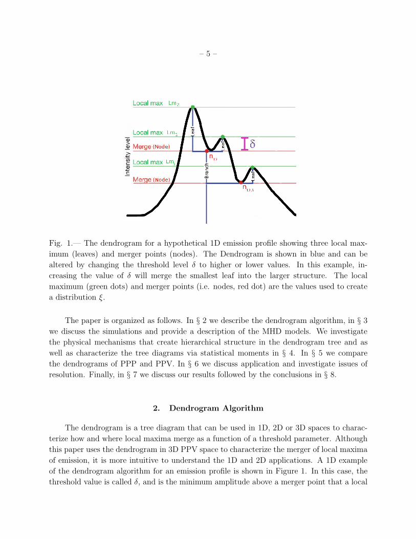
– 5 –

Fig. 1.— The dendrogram for a hypothetical 1D emission profile showing three local max-

imum (leaves) and merger points (nodes). The Dendrogram is shown in blue and can be

altered by changing the threshold level δ to higher or lower values. In this example, in-

creasing the value of δ will merge the smallest leaf into the larger structure. The local

maximum (green dots) and merger points (i.e. nodes, red dot) are the values used to create

a distribution ξ.

The paper is organized as follows. In § 2 we describe the dendrogram algorithm, in § 3

we discuss the simulations and provide a description of the MHD models. We investigate

the physical mechanisms that create hierarchical structure in the dendrogram tree and as

well as characterize the tree diagrams via statistical moments in § 4. In § 5 we compare

the dendrograms of PPP and PPV. In § 6 we discuss application and investigate issues of

resolution. Finally, in § 7 we discuss our results followed by the conclusions in § 8.

2. Dendrogram Algorithm

The dendrogram is a tree diagram that can be used in 1D, 2D or 3D spaces to charac-

terize how and where local maxima merge as a function of a threshold parameter. Although

this paper uses the dendrogram in 3D PPV space to characterize the merger of local maxima

of emission, it is more intuitive to understand the 1D and 2D applications. A 1D example

of the dendrogram algorithm for an emission profile is shown in Figure 1. In this case, the

threshold value is called δ, and is the minimum amplitude above a merger point that a local

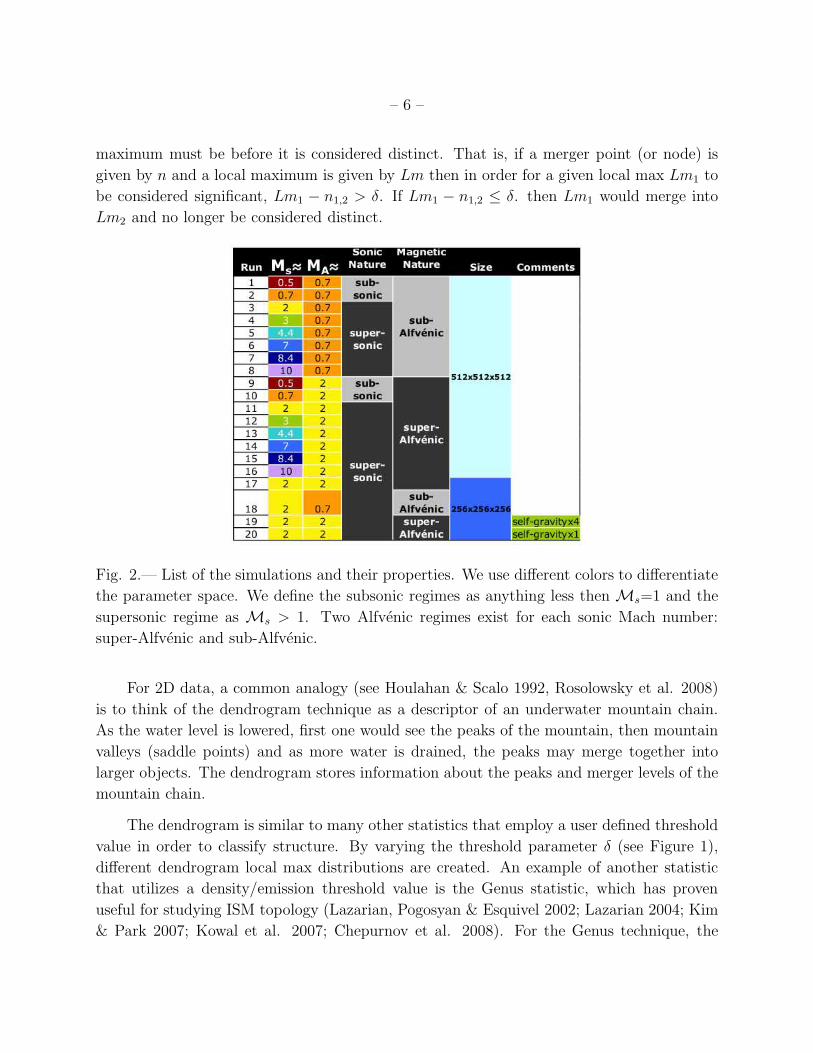
– 6 –

maximum must be before it is considered distinct. That is, if a merger point (or node) is

given by n and a local maximum is given by Lm then in order for a given local max Lm1 to

be considered significant, Lm1 − n1,2 > δ. If Lm1 − n1,2 ≤ δ. then Lm1 would merge into

Lm2 and no longer be considered distinct.

Fig. 2.— List of the simulations and their properties. We use different colors to differentiate

the parameter space. We define the subsonic regimes as anything less then Ms=1 and the

supersonic regime as Ms > 1. Two Alfvenic regimes exist for each sonic Mach number:

super-Alfvenic and sub-Alfvenic.

For 2D data, a common analogy (see Houlahan & Scalo 1992, Rosolowsky et al. 2008)

is to think of the dendrogram technique as a descriptor of an underwater mountain chain.

As the water level is lowered, first one would see the peaks of the mountain, then mountain

valleys (saddle points) and as more water is drained, the peaks may merge together into

larger objects. The dendrogram stores information about the peaks and merger levels of the

mountain chain.

The dendrogram is similar to many other statistics that employ a user defined threshold

value in order to classify structure. By varying the threshold parameter δ (see Figure 1),

different dendrogram local max distributions are created. An example of another statistic

that utilizes a density/emission threshold value is the Genus statistic, which has proven

useful for studying ISM topology (Lazarian, Pogosyan & Esquivel 2002; Lazarian 2004; Kim

& Park 2007; Kowal et al. 2007; Chepurnov et al. 2008). For the Genus technique, the

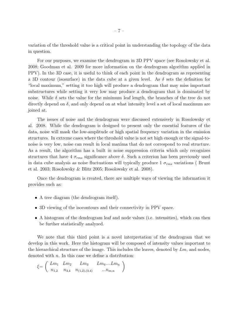
– 7 –

variation of the threshold value is a critical point in understanding the topology of the data

in question.

For our purposes, we examine the dendrogram in 3D PPV space (see Rosolowsky et al.

2008; Goodman et al. 2009 for more information on the dendrogram algorithm applied in

PPV). In the 3D case, it is useful to think of each point in the dendrogram as representing

a 3D contour (isosurface) in the data cube at a given level. As δ sets the definition for

“local maximum,” setting it too high will produce a dendrogram that may miss important

substructures while setting it very low may produce a dendrogram that is dominated by

noise. While δ sets the value for the minimum leaf length, the branches of the tree do not

directly depend on δ, and only depend on at what intensity level a set of local maximum are

joined at.

The issues of noise and the dendrogram were discussed extensively in Rosolowsky et

al. 2008. While the dendrogram is designed to present only the essential features of the

data, noise will mask the low-amplitude or high spatial frequency variation in the emission

structures. In extreme cases where the threshold value is not set high enough or the signal-to-

noise is very low, noise can result in local maxima that do not correspond to real structure.

As a result, the algorithm has a built in noise suppression criteria which only recognizes

structures that have 4 σrms significance above δ. Such a criterion has been previously used

in data cube analysis as noise fluctuations will typically produce 1 σrms variations ( Brunt

et al. 2003; Rosolowsky & Blitz 2005; Rosolowsky et al. 2008).

Once the dendrogram is created, there are multiple ways of viewing the information it

provides such as:

• A tree diagram (the dendrogram itself).

• 3D viewing of the isocontours and their connectivity in PPV space.

• A histogram of the dendrogram leaf and node values (i.e. intensities), which can then

be further statistically analyzed.

We note that this third point is a novel interpretation of the dendrogram that we

develop in this work. Here the histogram will be composed of intensity values important to

the hierarchical structure of the image. This includes the leaves, denoted by Lm, and nodes,

denoted with n. In this case we define a distribution:

ξ=

(

Lm1 Lm2 Lm3 Lm4....Lmn

n1,2 n3,4 n(1,2),(3,4) ...nm,n

)

– 8 –

This interpretation is visualized in Figure 3 and further described below. To produce

the dendrogram, we first identify a population of local maxima as the points which are

larger than all surrounding voxels touching along the face (not along edges or corners). This

large set of local maxima is then reduced by examining each maximum and searching for

the smallest contour level that contains only that maximum. If this contour level is less

than δ below the local maximum, that local maximum is removed from consideration in the

leaf population (this difference in data values is the vertical length of the “leaves” of the

dendrogram).

Once the leaves (local maxima) of the dendrogram are established, we contour the data

with a large number of levels (500 specifically, see Rosolowsky et al. 2008; Goodman et al.

2009). The dendrogram “branches” are graphically constructed by connecting the various

sets of maxima at the contour levels where they are joined (see Figure 1 for a 1D example).

For graphical presentation, the leaves of the structure tree are shuffled until the branches do

not cross when plotting. As a result, the x-axis of the dendrogram contains no information.

More information on the dendrogram algorithm can be found in Goodman et al. (2009) in

the Supplementary Methods section and in Rosolowsky et al. (2008).

The purpose of this paper is to use dendrogram to characterize the observed hierarchy

seen in the data. We are not necessarily interested in individual clumps found in the synthetic

PPV data, but rather characterizing how the structures and hierarchy found in simulations of

MHD turbulence depend on parameters such as the level of turbulence, magnetic fields, and

self-gravity. While turbulence has often been cited as the cause of the observed hierarchical

structure in the ISM (Stutzki 1998), it is unclear to what extent magnetic fields, gas pressure,

and gravity play roles in the creation of ISM hierarchy even though these parameters are

known to drastically change the PDF and spectrum of both column density and PPV data

(see Falgarone 1994; Kowal et al. 2007; Tofflemire et al. 2011).

3. Data

We generate a database of twenty 3D numerical simulations of isothermal compressible

(MHD) turbulence by using the MHD code of Cho & Lazarian 2003 and vary the input

values for the sonic and Alfvenic Mach number. We briefly outline the major points of the

numerical setup.

The code is a second-order-accurate hybrid essentially non-oscillatory (ENO) scheme

which solves the ideal MHD equations in a periodic box:

∂ρ

∂t+∇ · (ρv) = 0, (1)

– 9 –

∂ρv

∂t+∇ ·

[

ρvv +

(

p+B2

8π

)

I−1

4πBB

]

= f , (2)

∂B

∂t−∇× (v ×B) = 0, (3)

with zero-divergence condition ∇ · B = 0, and an isothermal equation of state p = C2sρ,

where p is the gas pressure. On the right-hand side, the source term f is a random large-

scale driving force. We drive turbulence solenoidally2 with energy injected on the large scales.

The time t is in units of the large eddy turnover time (∼ L/δV ) and the length in units of

L, the scale of energy injection. The magnetic field consists of the uniform background field

and a fluctuating field: B = Bext + b. Initially b = 0. We stress that simulations are scale

free and all units are related to the turnover time and energy injection scale.

We divide our models into two groups corresponding to sub-Alfvenic and super-Alfvenic

turbulence. For each group we computed several models with different values of gas pressure

(see Figure 2) falling into regimes of sub-sonic and supersonic. We ran 14 compressible MHD

turbulent models, with 5123 resolution, and 4 at 2563 with 2 of these having self-gravity. We

solve for the gravitation potential using a Fourier method similar to that described in Ostriker

et al. 1999. The models are listed and described in Figure 2.

We use density and velocity perpendicular to the mean magnetic field in order to create

fully optically thin synthetic PPV data cubes, although we also investigate dendrogram for

other LOS orientations. The PPP and synthetic PPV cubes are all normalized by the mean

value, i.e. PPVfinal = PPVorignial/ < PPVorignial >) Varying the optical depth will be

done in a later work. We create cubes with a given velocity resolution of 0.07, which is

ten times smaller then the rms velocity of the simulation (vrms = 0.7). For reference, the

sound speed of the simulations varies from cs = 1.4 − 0.07 for our most subsonic to most

supersonic simulations. PPV cubes are created by reorganizing density cubes into channel

bins based on given velocity intervals. Additional discussion on comparing the simulations

to observations is found in Section 6.

2The differences between solenoidal and compressive driving is discussed more in Federrath et al. 2008.

One can expect driving in the ISM to be a combination of solenoidal and compressive, however both types

of driving will produce shocks on a range of scales, which is what we study here.

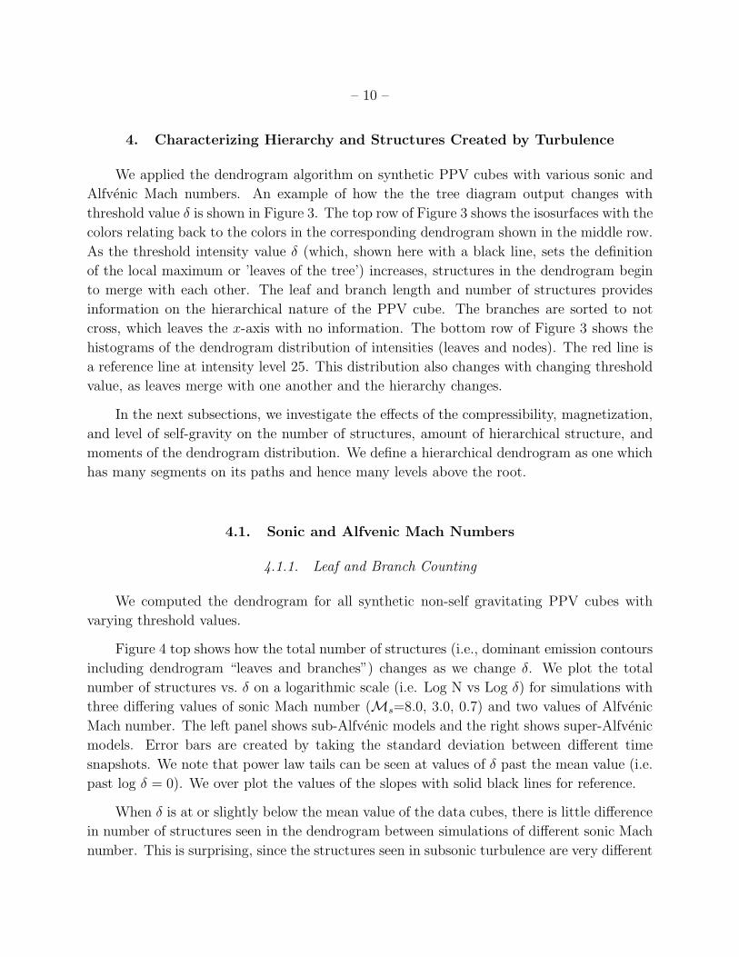
– 10 –

4. Characterizing Hierarchy and Structures Created by Turbulence

We applied the dendrogram algorithm on synthetic PPV cubes with various sonic and

Alfvenic Mach numbers. An example of how the the tree diagram output changes with

threshold value δ is shown in Figure 3. The top row of Figure 3 shows the isosurfaces with the

colors relating back to the colors in the corresponding dendrogram shown in the middle row.

As the threshold intensity value δ (which, shown here with a black line, sets the definition

of the local maximum or ’leaves of the tree’) increases, structures in the dendrogram begin

to merge with each other. The leaf and branch length and number of structures provides

information on the hierarchical nature of the PPV cube. The branches are sorted to not

cross, which leaves the x-axis with no information. The bottom row of Figure 3 shows the

histograms of the dendrogram distribution of intensities (leaves and nodes). The red line is

a reference line at intensity level 25. This distribution also changes with changing threshold

value, as leaves merge with one another and the hierarchy changes.

In the next subsections, we investigate the effects of the compressibility, magnetization,

and level of self-gravity on the number of structures, amount of hierarchical structure, and

moments of the dendrogram distribution. We define a hierarchical dendrogram as one which

has many segments on its paths and hence many levels above the root.

4.1. Sonic and Alfvenic Mach Numbers

4.1.1. Leaf and Branch Counting

We computed the dendrogram for all synthetic non-self gravitating PPV cubes with

varying threshold values.

Figure 4 top shows how the total number of structures (i.e., dominant emission contours

including dendrogram “leaves and branches”) changes as we change δ. We plot the total

number of structures vs. δ on a logarithmic scale (i.e. Log N vs Log δ) for simulations with

three differing values of sonic Mach number (Ms=8.0, 3.0, 0.7) and two values of Alfvenic

Mach number. The left panel shows sub-Alfvenic models and the right shows super-Alfvenic

models. Error bars are created by taking the standard deviation between different time

snapshots. We note that power law tails can be seen at values of δ past the mean value (i.e.

past log δ = 0). We over plot the values of the slopes with solid black lines for reference.

When δ is at or slightly below the mean value of the data cubes, there is little difference

in number of structures seen in the dendrogram between simulations of different sonic Mach

number. This is surprising, since the structures seen in subsonic turbulence are very different

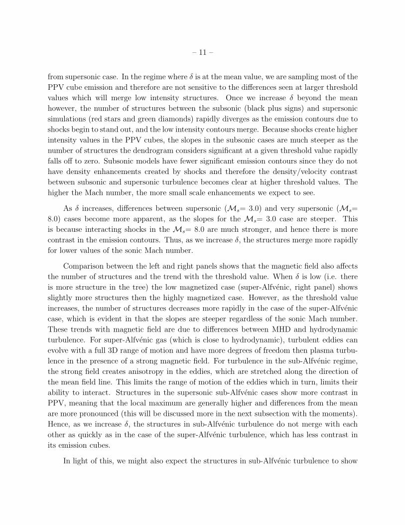
– 11 –

from supersonic case. In the regime where δ is at the mean value, we are sampling most of the

PPV cube emission and therefore are not sensitive to the differences seen at larger threshold

values which will merge low intensity structures. Once we increase δ beyond the mean

however, the number of structures between the subsonic (black plus signs) and supersonic

simulations (red stars and green diamonds) rapidly diverges as the emission contours due to

shocks begin to stand out, and the low intensity contours merge. Because shocks create higher

intensity values in the PPV cubes, the slopes in the subsonic cases are much steeper as the

number of structures the dendrogram considers significant at a given threshold value rapidly

falls off to zero. Subsonic models have fewer significant emission contours since they do not

have density enhancements created by shocks and therefore the density/velocity contrast

between subsonic and supersonic turbulence becomes clear at higher threshold values. The

higher the Mach number, the more small scale enhancements we expect to see.

As δ increases, differences between supersonic (Ms= 3.0) and very supersonic (Ms=

8.0) cases become more apparent, as the slopes for the Ms= 3.0 case are steeper. This

is because interacting shocks in the Ms= 8.0 are much stronger, and hence there is more

contrast in the emission contours. Thus, as we increase δ, the structures merge more rapidly

for lower values of the sonic Mach number.

Comparison between the left and right panels shows that the magnetic field also affects

the number of structures and the trend with the threshold value. When δ is low (i.e. there

is more structure in the tree) the low magnetized case (super-Alfvenic, right panel) shows

slightly more structures then the highly magnetized case. However, as the threshold value

increases, the number of structures decreases more rapidly in the case of the super-Alfvenic

case, which is evident in that the slopes are steeper regardless of the sonic Mach number.

These trends with magnetic field are due to differences between MHD and hydrodynamic

turbulence. For super-Alfvenic gas (which is close to hydrodynamic), turbulent eddies can

evolve with a full 3D range of motion and have more degrees of freedom then plasma turbu-

lence in the presence of a strong magnetic field. For turbulence in the sub-Alfvenic regime,

the strong field creates anisotropy in the eddies, which are stretched along the direction of

the mean field line. This limits the range of motion of the eddies which in turn, limits their

ability to interact. Structures in the supersonic sub-Alfvenic cases show more contrast in

PPV, meaning that the local maximum are generally higher and differences from the mean

are more pronounced (this will be discussed more in the next subsection with the moments).

Hence, as we increase δ, the structures in sub-Alfvenic turbulence do not merge with each

other as quickly as in the case of the super-Alfvenic turbulence, which has less contrast in

its emission cubes.

In light of this, we might also expect the structures in sub-Alfvenic turbulence to show

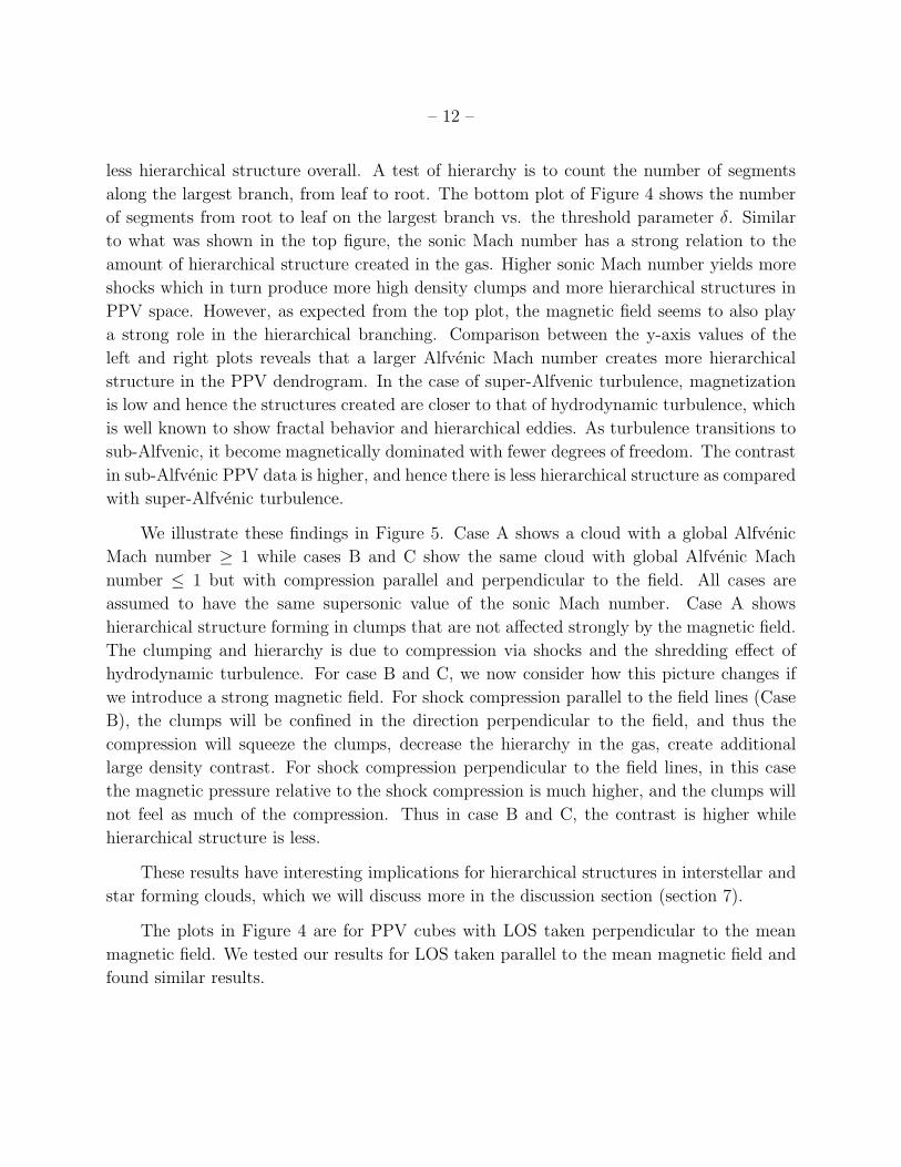
– 12 –

less hierarchical structure overall. A test of hierarchy is to count the number of segments

along the largest branch, from leaf to root. The bottom plot of Figure 4 shows the number

of segments from root to leaf on the largest branch vs. the threshold parameter δ. Similar

to what was shown in the top figure, the sonic Mach number has a strong relation to the

amount of hierarchical structure created in the gas. Higher sonic Mach number yields more

shocks which in turn produce more high density clumps and more hierarchical structures in

PPV space. However, as expected from the top plot, the magnetic field seems to also play

a strong role in the hierarchical branching. Comparison between the y-axis values of the

left and right plots reveals that a larger Alfvenic Mach number creates more hierarchical

structure in the PPV dendrogram. In the case of super-Alfvenic turbulence, magnetization

is low and hence the structures created are closer to that of hydrodynamic turbulence, which

is well known to show fractal behavior and hierarchical eddies. As turbulence transitions to

sub-Alfvenic, it become magnetically dominated with fewer degrees of freedom. The contrast

in sub-Alfvenic PPV data is higher, and hence there is less hierarchical structure as compared

with super-Alfvenic turbulence.

We illustrate these findings in Figure 5. Case A shows a cloud with a global Alfvenic

Mach number ≥ 1 while cases B and C show the same cloud with global Alfvenic Mach

number ≤ 1 but with compression parallel and perpendicular to the field. All cases are

assumed to have the same supersonic value of the sonic Mach number. Case A shows

hierarchical structure forming in clumps that are not affected strongly by the magnetic field.

The clumping and hierarchy is due to compression via shocks and the shredding effect of

hydrodynamic turbulence. For case B and C, we now consider how this picture changes if

we introduce a strong magnetic field. For shock compression parallel to the field lines (Case

B), the clumps will be confined in the direction perpendicular to the field, and thus the

compression will squeeze the clumps, decrease the hierarchy in the gas, create additional

large density contrast. For shock compression perpendicular to the field lines, in this case

the magnetic pressure relative to the shock compression is much higher, and the clumps will

not feel as much of the compression. Thus in case B and C, the contrast is higher while

hierarchical structure is less.

These results have interesting implications for hierarchical structures in interstellar and

star forming clouds, which we will discuss more in the discussion section (section 7).

The plots in Figure 4 are for PPV cubes with LOS taken perpendicular to the mean

magnetic field. We tested our results for LOS taken parallel to the mean magnetic field and

found similar results.

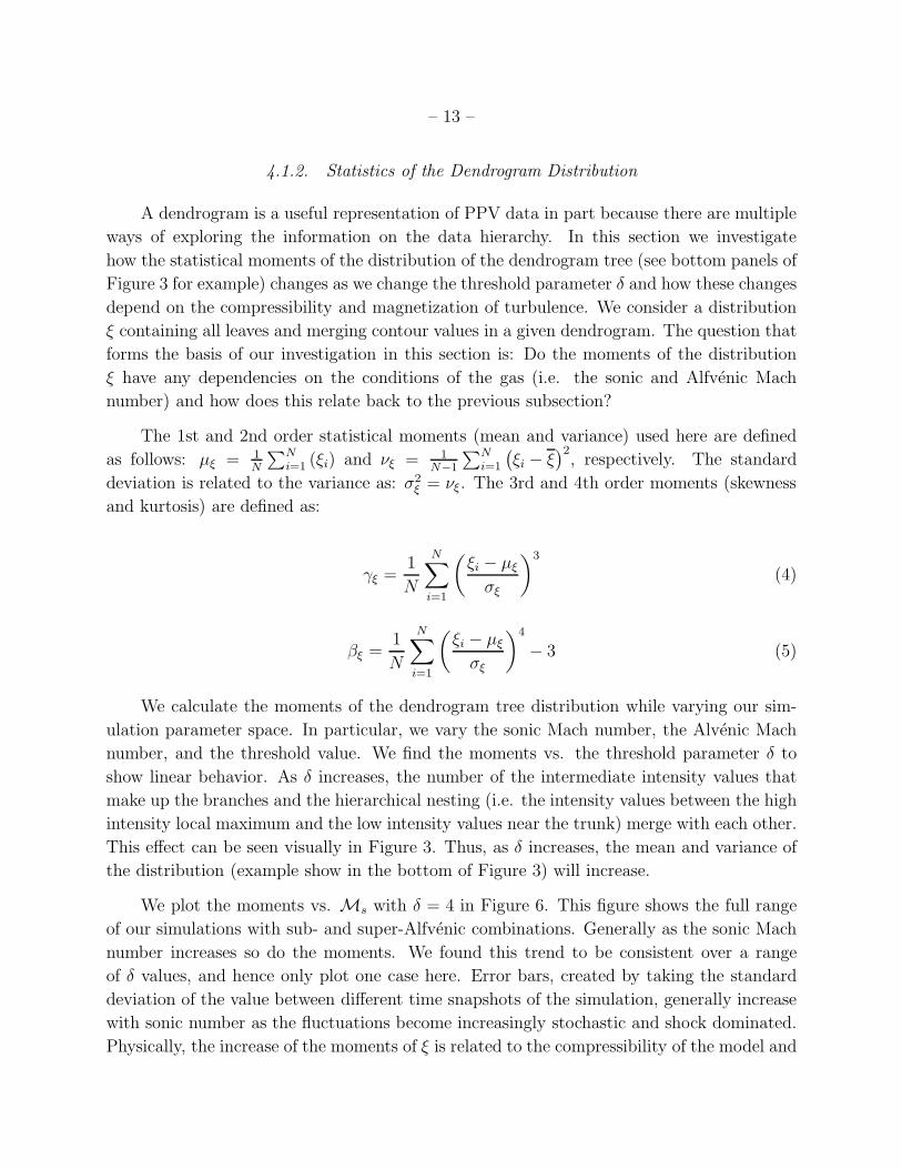
– 13 –

4.1.2. Statistics of the Dendrogram Distribution

A dendrogram is a useful representation of PPV data in part because there are multiple

ways of exploring the information on the data hierarchy. In this section we investigate

how the statistical moments of the distribution of the dendrogram tree (see bottom panels of

Figure 3 for example) changes as we change the threshold parameter δ and how these changes

depend on the compressibility and magnetization of turbulence. We consider a distribution

ξ containing all leaves and merging contour values in a given dendrogram. The question that

forms the basis of our investigation in this section is: Do the moments of the distribution

ξ have any dependencies on the conditions of the gas (i.e. the sonic and Alfvenic Mach

number) and how does this relate back to the previous subsection?

The 1st and 2nd order statistical moments (mean and variance) used here are defined

as follows: µξ = 1N

∑N

i=1 (ξi) and νξ = 1N−1

∑N

i=1

(

ξi − ξ)2, respectively. The standard

deviation is related to the variance as: σ2ξ = νξ. The 3rd and 4th order moments (skewness

and kurtosis) are defined as:

γξ =1

N

N∑

i=1

(

ξi − µξ

σξ

)3

(4)

βξ =1

N

N∑

i=1

(

ξi − µξ

σξ

)4

− 3 (5)

We calculate the moments of the dendrogram tree distribution while varying our sim-

ulation parameter space. In particular, we vary the sonic Mach number, the Alvenic Mach

number, and the threshold value. We find the moments vs. the threshold parameter δ to

show linear behavior. As δ increases, the number of the intermediate intensity values that

make up the branches and the hierarchical nesting (i.e. the intensity values between the high

intensity local maximum and the low intensity values near the trunk) merge with each other.

This effect can be seen visually in Figure 3. Thus, as δ increases, the mean and variance of

the distribution (example show in the bottom of Figure 3) will increase.

We plot the moments vs. Ms with δ = 4 in Figure 6. This figure shows the full range

of our simulations with sub- and super-Alfvenic combinations. Generally as the sonic Mach

number increases so do the moments. We found this trend to be consistent over a range

of δ values, and hence only plot one case here. Error bars, created by taking the standard

deviation of the value between different time snapshots of the simulation, generally increase

with sonic number as the fluctuations become increasingly stochastic and shock dominated.

Physically, the increase of the moments of ξ is related to the compressibility of the model and

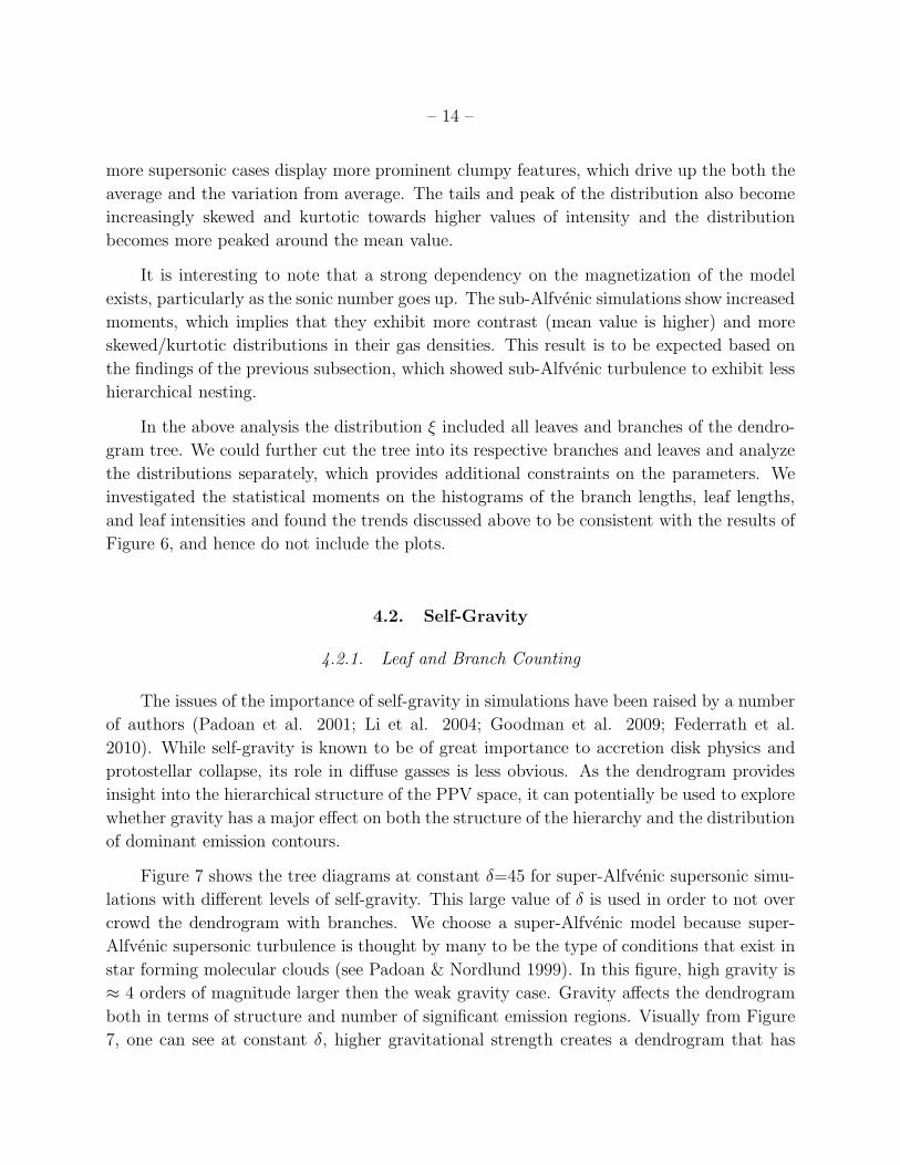
– 14 –

more supersonic cases display more prominent clumpy features, which drive up the both the

average and the variation from average. The tails and peak of the distribution also become

increasingly skewed and kurtotic towards higher values of intensity and the distribution

becomes more peaked around the mean value.

It is interesting to note that a strong dependency on the magnetization of the model

exists, particularly as the sonic number goes up. The sub-Alfvenic simulations show increased

moments, which implies that they exhibit more contrast (mean value is higher) and more

skewed/kurtotic distributions in their gas densities. This result is to be expected based on

the findings of the previous subsection, which showed sub-Alfvenic turbulence to exhibit less

hierarchical nesting.

In the above analysis the distribution ξ included all leaves and branches of the dendro-

gram tree. We could further cut the tree into its respective branches and leaves and analyze

the distributions separately, which provides additional constraints on the parameters. We

investigated the statistical moments on the histograms of the branch lengths, leaf lengths,

and leaf intensities and found the trends discussed above to be consistent with the results of

Figure 6, and hence do not include the plots.

4.2. Self-Gravity

4.2.1. Leaf and Branch Counting

The issues of the importance of self-gravity in simulations have been raised by a number

of authors (Padoan et al. 2001; Li et al. 2004; Goodman et al. 2009; Federrath et al.

2010). While self-gravity is known to be of great importance to accretion disk physics and

protostellar collapse, its role in diffuse gasses is less obvious. As the dendrogram provides

insight into the hierarchical structure of the PPV space, it can potentially be used to explore

whether gravity has a major effect on both the structure of the hierarchy and the distribution

of dominant emission contours.

Figure 7 shows the tree diagrams at constant δ=45 for super-Alfvenic supersonic simu-

lations with different levels of self-gravity. This large value of δ is used in order to not over

crowd the dendrogram with branches. We choose a super-Alfvenic model because super-

Alfvenic supersonic turbulence is thought by many to be the type of conditions that exist in

star forming molecular clouds (see Padoan & Nordlund 1999). In this figure, high gravity is

≈ 4 orders of magnitude larger then the weak gravity case. Gravity affects the dendrogram

both in terms of structure and number of significant emission regions. Visually from Figure

7, one can see at constant δ, higher gravitational strength creates a dendrogram that has

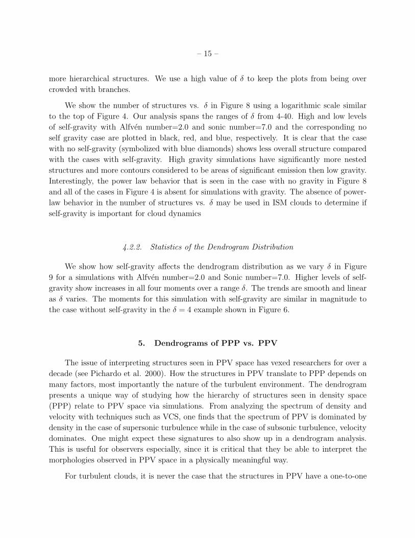
– 15 –

more hierarchical structures. We use a high value of δ to keep the plots from being over

crowded with branches.

We show the number of structures vs. δ in Figure 8 using a logarithmic scale similar

to the top of Figure 4. Our analysis spans the ranges of δ from 4-40. High and low levels

of self-gravity with Alfven number=2.0 and sonic number=7.0 and the corresponding no

self gravity case are plotted in black, red, and blue, respectively. It is clear that the case

with no self-gravity (symbolized with blue diamonds) shows less overall structure compared

with the cases with self-gravity. High gravity simulations have significantly more nested

structures and more contours considered to be areas of significant emission then low gravity.

Interestingly, the power law behavior that is seen in the case with no gravity in Figure 8

and all of the cases in Figure 4 is absent for simulations with gravity. The absence of power-

law behavior in the number of structures vs. δ may be used in ISM clouds to determine if

self-gravity is important for cloud dynamics

4.2.2. Statistics of the Dendrogram Distribution

We show how self-gravity affects the dendrogram distribution as we vary δ in Figure

9 for a simulations with Alfven number=2.0 and Sonic number=7.0. Higher levels of self-

gravity show increases in all four moments over a range δ. The trends are smooth and linear

as δ varies. The moments for this simulation with self-gravity are similar in magnitude to

the case without self-gravity in the δ = 4 example shown in Figure 6.

5. Dendrograms of PPP vs. PPV

The issue of interpreting structures seen in PPV space has vexed researchers for over a

decade (see Pichardo et al. 2000). How the structures in PPV translate to PPP depends on

many factors, most importantly the nature of the turbulent environment. The dendrogram

presents a unique way of studying how the hierarchy of structures seen in density space

(PPP) relate to PPV space via simulations. From analyzing the spectrum of density and

velocity with techniques such as VCS, one finds that the spectrum of PPV is dominated by

density in the case of supersonic turbulence while in the case of subsonic turbulence, velocity

dominates. One might expect these signatures to also show up in a dendrogram analysis.

This is useful for observers especially, since it is critical that they be able to interpret the

morphologies observed in PPV space in a physically meaningful way.

For turbulent clouds, it is never the case that the structures in PPV have a one-to-one

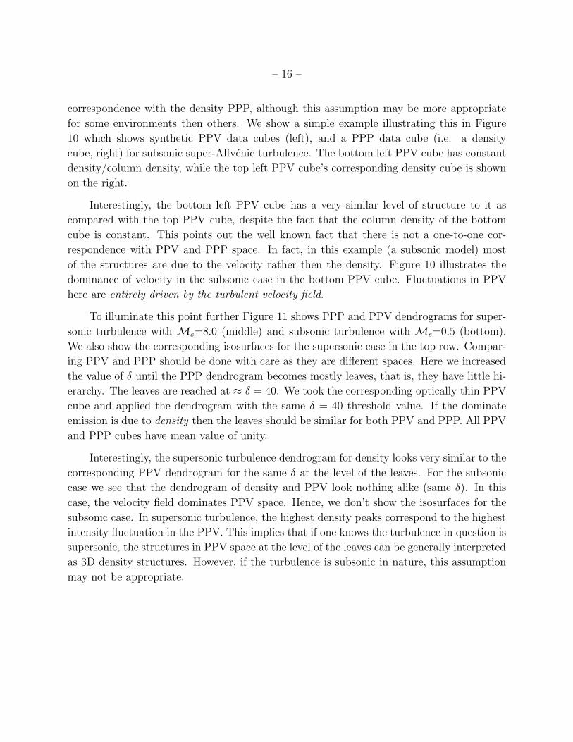
– 16 –

correspondence with the density PPP, although this assumption may be more appropriate

for some environments then others. We show a simple example illustrating this in Figure

10 which shows synthetic PPV data cubes (left), and a PPP data cube (i.e. a density

cube, right) for subsonic super-Alfvenic turbulence. The bottom left PPV cube has constant

density/column density, while the top left PPV cube’s corresponding density cube is shown

on the right.

Interestingly, the bottom left PPV cube has a very similar level of structure to it as

compared with the top PPV cube, despite the fact that the column density of the bottom

cube is constant. This points out the well known fact that there is not a one-to-one cor-

respondence with PPV and PPP space. In fact, in this example (a subsonic model) most

of the structures are due to the velocity rather then the density. Figure 10 illustrates the

dominance of velocity in the subsonic case in the bottom PPV cube. Fluctuations in PPV

here are entirely driven by the turbulent velocity field.

To illuminate this point further Figure 11 shows PPP and PPV dendrograms for super-

sonic turbulence with Ms=8.0 (middle) and subsonic turbulence with Ms=0.5 (bottom).

We also show the corresponding isosurfaces for the supersonic case in the top row. Compar-

ing PPV and PPP should be done with care as they are different spaces. Here we increased

the value of δ until the PPP dendrogram becomes mostly leaves, that is, they have little hi-

erarchy. The leaves are reached at ≈ δ = 40. We took the corresponding optically thin PPV

cube and applied the dendrogram with the same δ = 40 threshold value. If the dominate

emission is due to density then the leaves should be similar for both PPV and PPP. All PPV

and PPP cubes have mean value of unity.

Interestingly, the supersonic turbulence dendrogram for density looks very similar to the

corresponding PPV dendrogram for the same δ at the level of the leaves. For the subsonic

case we see that the dendrogram of density and PPV look nothing alike (same δ). In this

case, the velocity field dominates PPV space. Hence, we don’t show the isosurfaces for the

subsonic case. In supersonic turbulence, the highest density peaks correspond to the highest

intensity fluctuation in the PPV. This implies that if one knows the turbulence in question is

supersonic, the structures in PPV space at the level of the leaves can be generally interpreted

as 3D density structures. However, if the turbulence is subsonic in nature, this assumption

may not be appropriate.

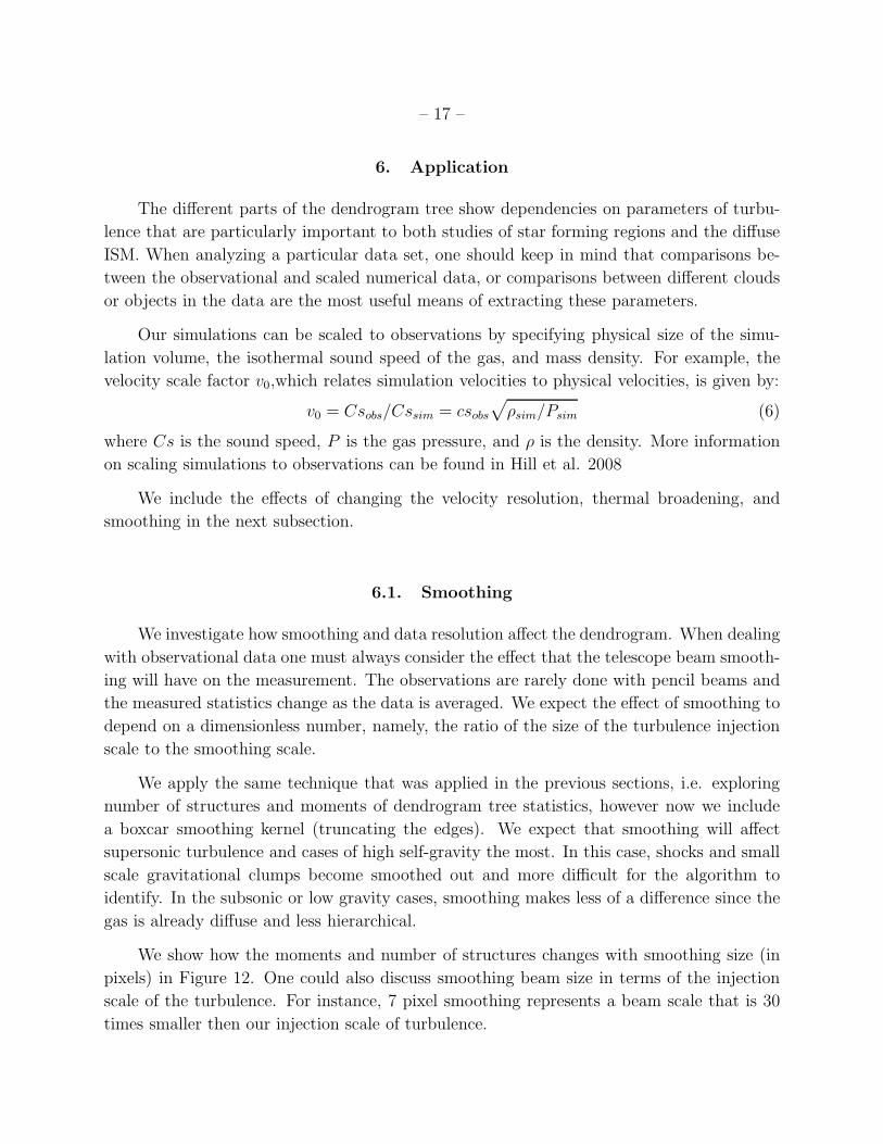
– 17 –

6. Application

The different parts of the dendrogram tree show dependencies on parameters of turbu-

lence that are particularly important to both studies of star forming regions and the diffuse

ISM. When analyzing a particular data set, one should keep in mind that comparisons be-

tween the observational and scaled numerical data, or comparisons between different clouds

or objects in the data are the most useful means of extracting these parameters.

Our simulations can be scaled to observations by specifying physical size of the simu-

lation volume, the isothermal sound speed of the gas, and mass density. For example, the

velocity scale factor v0,which relates simulation velocities to physical velocities, is given by:

v0 = Csobs/Cssim = csobs√

ρsim/Psim (6)

where Cs is the sound speed, P is the gas pressure, and ρ is the density. More information

on scaling simulations to observations can be found in Hill et al. 2008

We include the effects of changing the velocity resolution, thermal broadening, and

smoothing in the next subsection.

6.1. Smoothing

We investigate how smoothing and data resolution affect the dendrogram. When dealing

with observational data one must always consider the effect that the telescope beam smooth-

ing will have on the measurement. The observations are rarely done with pencil beams and

the measured statistics change as the data is averaged. We expect the effect of smoothing to

depend on a dimensionless number, namely, the ratio of the size of the turbulence injection

scale to the smoothing scale.

We apply the same technique that was applied in the previous sections, i.e. exploring

number of structures and moments of dendrogram tree statistics, however now we include

a boxcar smoothing kernel (truncating the edges). We expect that smoothing will affect

supersonic turbulence and cases of high self-gravity the most. In this case, shocks and small

scale gravitational clumps become smoothed out and more difficult for the algorithm to

identify. In the subsonic or low gravity cases, smoothing makes less of a difference since the

gas is already diffuse and less hierarchical.

We show how the moments and number of structures changes with smoothing size (in

pixels) in Figure 12. One could also discuss smoothing beam size in terms of the injection

scale of the turbulence. For instance, 7 pixel smoothing represents a beam scale that is 30

times smaller then our injection scale of turbulence.

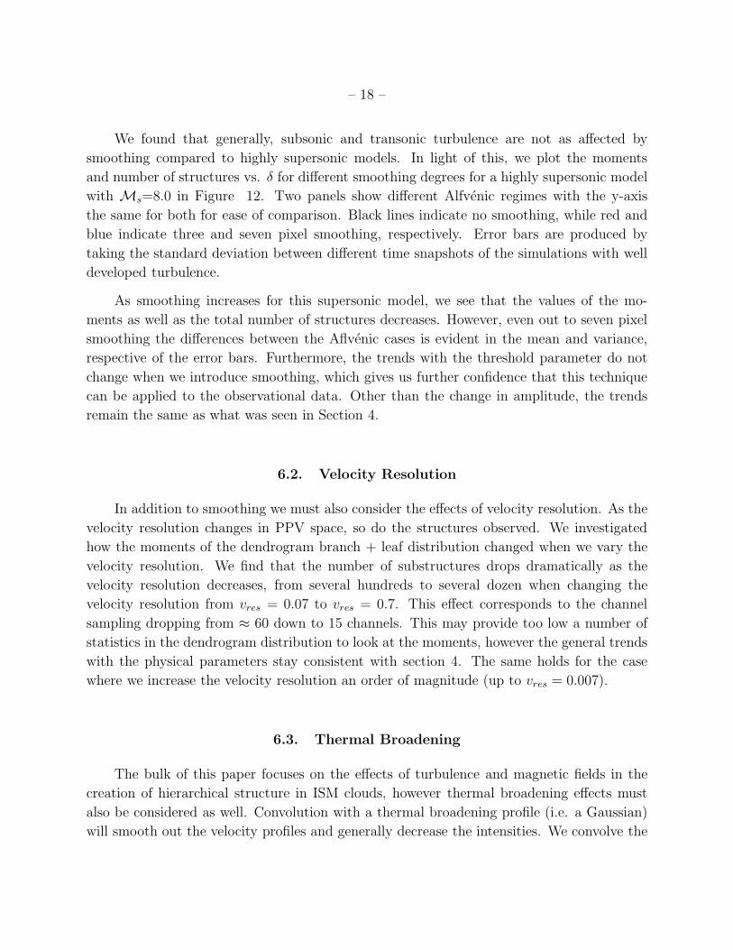
– 18 –

We found that generally, subsonic and transonic turbulence are not as affected by

smoothing compared to highly supersonic models. In light of this, we plot the moments

and number of structures vs. δ for different smoothing degrees for a highly supersonic model

with Ms=8.0 in Figure 12. Two panels show different Alfvenic regimes with the y-axis

the same for both for ease of comparison. Black lines indicate no smoothing, while red and

blue indicate three and seven pixel smoothing, respectively. Error bars are produced by

taking the standard deviation between different time snapshots of the simulations with well

developed turbulence.

As smoothing increases for this supersonic model, we see that the values of the mo-

ments as well as the total number of structures decreases. However, even out to seven pixel

smoothing the differences between the Aflvenic cases is evident in the mean and variance,

respective of the error bars. Furthermore, the trends with the threshold parameter do not

change when we introduce smoothing, which gives us further confidence that this technique

can be applied to the observational data. Other than the change in amplitude, the trends

remain the same as what was seen in Section 4.

6.2. Velocity Resolution

In addition to smoothing we must also consider the effects of velocity resolution. As the

velocity resolution changes in PPV space, so do the structures observed. We investigated

how the moments of the dendrogram branch + leaf distribution changed when we vary the

velocity resolution. We find that the number of substructures drops dramatically as the

velocity resolution decreases, from several hundreds to several dozen when changing the

velocity resolution from vres = 0.07 to vres = 0.7. This effect corresponds to the channel

sampling dropping from ≈ 60 down to 15 channels. This may provide too low a number of

statistics in the dendrogram distribution to look at the moments, however the general trends

with the physical parameters stay consistent with section 4. The same holds for the case

where we increase the velocity resolution an order of magnitude (up to vres = 0.007).

6.3. Thermal Broadening

The bulk of this paper focuses on the effects of turbulence and magnetic fields in the

creation of hierarchical structure in ISM clouds, however thermal broadening effects must

also be considered as well. Convolution with a thermal broadening profile (i.e. a Gaussian)

will smooth out the velocity profiles and generally decrease the intensities. We convolve the

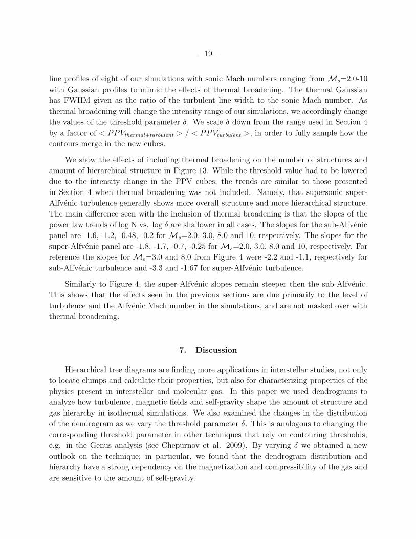
– 19 –

line profiles of eight of our simulations with sonic Mach numbers ranging from Ms=2.0-10

with Gaussian profiles to mimic the effects of thermal broadening. The thermal Gaussian

has FWHM given as the ratio of the turbulent line width to the sonic Mach number. As

thermal broadening will change the intensity range of our simulations, we accordingly change

the values of the threshold parameter δ. We scale δ down from the range used in Section 4

by a factor of < PPVthermal+turbulent > / < PPVturbulent >, in order to fully sample how the

contours merge in the new cubes.

We show the effects of including thermal broadening on the number of structures and

amount of hierarchical structure in Figure 13. While the threshold value had to be lowered

due to the intensity change in the PPV cubes, the trends are similar to those presented

in Section 4 when thermal broadening was not included. Namely, that supersonic super-

Alfvenic turbulence generally shows more overall structure and more hierarchical structure.

The main difference seen with the inclusion of thermal broadening is that the slopes of the

power law trends of log N vs. log δ are shallower in all cases. The slopes for the sub-Alfvenic

panel are -1.6, -1.2, -0.48, -0.2 for Ms=2.0, 3.0, 8.0 and 10, respectively. The slopes for the

super-Alfvenic panel are -1.8, -1.7, -0.7, -0.25 for Ms=2.0, 3.0, 8.0 and 10, respectively. For

reference the slopes for Ms=3.0 and 8.0 from Figure 4 were -2.2 and -1.1, respectively for

sub-Alfvenic turbulence and -3.3 and -1.67 for super-Alfvenic turbulence.

Similarly to Figure 4, the super-Alfvenic slopes remain steeper then the sub-Alfvenic.

This shows that the effects seen in the previous sections are due primarily to the level of

turbulence and the Alfvenic Mach number in the simulations, and are not masked over with

thermal broadening.

7. Discussion

Hierarchical tree diagrams are finding more applications in interstellar studies, not only

to locate clumps and calculate their properties, but also for characterizing properties of the

physics present in interstellar and molecular gas. In this paper we used dendrograms to

analyze how turbulence, magnetic fields and self-gravity shape the amount of structure and

gas hierarchy in isothermal simulations. We also examined the changes in the distribution

of the dendrogram as we vary the threshold parameter δ. This is analogous to changing the

corresponding threshold parameter in other techniques that rely on contouring thresholds,

e.g. in the Genus analysis (see Chepurnov et al. 2009). By varying δ we obtained a new

outlook on the technique; in particular, we found that the dendrogram distribution and

hierarchy have a strong dependency on the magnetization and compressibility of the gas and

are sensitive to the amount of self-gravity.

– 20 –

7.1. The Hierarchical Nature of MHD Turbulence

The number of structures and the amount of hierarchy formed by MHD turbulence has

interesting implications for the evolution of ISM clouds and for the star formation problem.

In section 4 we found that more hierarchical structure and more overall structure was created

in the presence of supersonic super-Alfvenic turbulence. We also found that the inclusion

of self-gravity enhanced these trends. The relationship between the magnetization and the

cloud dynamics is in the process of being understood, especially in regards to star formation.

Star forming clouds are known to be hierarchical in nature and magnetized, but the exact

Alfvenic nature is less clear. The results from this work seem to suggest that very hierar-

chical clouds might tend towards being super-Alfvenic. Several authors have suggested a

variety of evidence for molecular clouds being super-Alfvenic. This includes the agreement

of simulations and observations of Zeeman-splitting measurements, B vs.ρ relations, MA vs.

ρ relations, statistics of the extinction measurement etc. (Padoan & Nordlund 1999; Lunttila

et al. 2008; Burkhart et al. 2009; Crutcher et al. 2009; Collins et al. 2012). Furthermore a

study done by Burkhart et al. 2009 found that, even in the presence of globally sub-Alfvenic

turbulence, the highest density regions tend towards being locally super-Alfvenic. This sug-

gests that even in the case of globally sub-Alfvenic turbulence, the densest regions might be

super-Alfvenic. It is interesting that the dendrogram technique also points to super-Alfvenic

turbulence as an avenue for hierarchical structure creation. This provides motivation for the

dendrogram technique to be applied to the observational data with varying threshold value

δ in order to see how the nature of the hierarchical structure and total number of structures

change in the observations.

7.2. Sonic and Alfvenic Mach Numbers from the Observations

In the paper above we provided a systematic study of the variations of the dendrogram

δ with the sonic and magnetic Mach numbers. These numbers are critical for understanding

most of processes in galactic diffuse and molecular gas, including the process of star forma-

tion. Thus, the dendrogram provides an avenue of obtaining these parameters via comparing

observations and simulations and/or as a technique for investigating what processes are cre-

ating hierarchical structure in ISM gas.

We view this work as the springboard for applying the technique to the actual data.

We claim that for reliable studies of the interstellar media and molecular clouds it is most

advantageous to combine different techniques. For instance, applying the VCA and VCS

techniques to PPV data (see Lazarian 2009 for a review), one can obtain the velocity and

density spectra of turbulence. While these measures are known to depend on Ms and to a

– 21 –

lesser degree onMA (see Beresnyak, Lazarian & Cho 2005, Kowal et al. 2007, Burkhart et al.

2009), the utility of the spectra is not in measuring these quantities. Spectra provide a unique

way to investigate how the energy cascades between different scales, and shows whether

comparing observations with the simulations with a single scale of injection is reasonable.

The analysis of the anisotropies of correlations using velocity centroids provides an

insight into media magnetization, i.e., provides MA (Lazarian et al. 2002, Esquivel &

Lazarian 2005), which is complimentary to the technique described in this paper. Studies of

the skewness and kurtosis of the PDFs (see Kowal et al. 2007, Burkhart et al. 2009, 2010)

provides measures of the sonic Mach number Ms. Similarly, Tsallis statistics measures

(Esquivel & Lazarian 2010, Tofflemire et al. 2011) provide additional ways of estimating

both Ms and MA. We feel the approach to obtaining these parameters should be conducted

with synergetic use of multiple tools, such as was done in Burkhart et al. 2010 on the SMC.

We feel the dendrogram is a unique tool as it can classify the hierarchical nature of the data

and that it should be added to a standard set of statistical-tools for studies of ISM data.

All these techniques provide independent ways of evaluating parameters of turbulence

and therefore their application to the same data set provides a more reliable estimate of key

parameters such as compressibility, magnetization, and degree of self-gravity. Dendrograms

have some advantages over other statistics designed to search for turbulence parameters, in

that one can analyze the resulting tree diagram in many different ways, as highlighted in

this paper and in previous works. These include finding local maxima, calculating physical

properties of dominate emission, exploring how those clumps are connected in PPV, varying

the threshold and calculating moments and level of hierarchy. Of course, one should keep

in mind that the medium that we investigate observationally is far from simple. Multiple

energy injection sources, for example, are not excluded. Thus obtaining a similar answer

with different techniques should provide us with additional confidence in our results.

Finally, we should stress, that for studies of astrophysical objects the dendrogram and

other statistical measures can be applied locally to different parts of the media. For instance,

Burkhart et al. (2010) did not characterize the entire SMC with one sonic Mach number.

Instead, several measures were applied to parts of the SMC in order to obtain a distribution

of the turbulence in the galaxy. A similar local scale selection was applied also to the SMC

in Chepurnov et al. (2008) using the Genus technique. The same technique should be

used to parts of the ISM in the Milky way and may be attempted for GMCs. Correlating

the variations of the turbulence properties with observed properties of the media, e.g. star

formation rate should provide insight into how turbulence regulates many key astrophysical

processes.

– 22 –

8. Summary

We apply dendrograms to isothermal MHD simulations with varying levels of gravity,

compressibility and magnetization. We find that the dendrogram is a promising tool for

studying both gas connectivity in the ISM as well as characterizing turbulence. In particular

we find that:

• We propose using statistical descriptions of dendrograms as a means to quantify the

degree of hierarchy present in a PPV data cube.

• Shocks, self-gravity, and super-Alfvenic turbulence create the most hierarchical struc-

ture in PPV space.

• The number of dendrogram structures depends primarily on the sonic number and the

level of self-gravity and secondarily on the global magnetization.

• The first four statistical moments of the distribution of dendrogram leaves and con-

necting have monotonic dependencies on the level of self-gravity and the sonic and

Alfven Mach numbers over a range of δ.

• The dendrogram provides a convenient way of comparing PPP to PPV in simulations.

Density structures are dominant in supersonic PPV and not in subsonic. Thus it

is more justifiable to compare PPV directly to PPP when the gas is known to be

supersonic.

B.B. acknowledges support from the NSF Graduate Research Fellowship and the NASA

Wisconsin Space Grant Institution. B.B. is thankful for valuable discussions and the use of

the Dendrogui code via Chris Beaumont. A.L. thanks NSF AST 0808118, the Center for

Magnetic Self-Organization in Astrophysical and Laboratory Plasmas for financial support.

This work was completed during the stay of A.L. as Alexander-von-Humboldt-Preistrager

at the Ruhr-University Bochum. A.G. acknowledges support from NSF Grant No. AST-

0908159. E.R. is supported by a Discovery Grant from NSERC of Canada.

REFERENCES

Armstrong,J. W., Rickett, B. J., Spangler, S. R., 1995, ApJ, 443, 209

– 23 –

Ballesteros-Paredes, J., Klessen, R. S., Mac Low, M.-M., & Vazquez-Semadeni, E. 2007, in

Protostars and Planets V, ed. B. Reipurth, D. Jewitt, & K. Keil (Tucson, AZ: Univ.

of Arizona Press), 63

Beresnyak, A., Lazarian, A., Cho, J., 2005, ApJ, 624, 93

Berkhuijsen E., Fletcher, A., 2008, MNRAS, 390, 19

Brunt, C. M., Kerton, C. R., & Pomerleau, C., 2003, ApJS, 144, 47

Brunt, C., & Heyer, M., 2002, ApJ, 566, 27

Brunt, C., 2010, A&A, 513, 67

Burkhart, B., Falceta-Goncalves, D., Kowal, G., Lazarian, A., 2009, ApJ, 693, 250

Burkhart, B., Stanimirovic, S., Lazarian, A., Grzegorz, K., 2010, ApJ, 708, 1204

Burkhart, B., Lazarian, A., Gaensler, B., 2012, ApJ, 708, 1204

Burkhart, B., & Lazarian, A., 2011, IAUS, 274, 365

Chepurnov, A., Gordon, J., Lazarian, A., & Stanimirovic, S.,2008, ApJ, 688, 1021

Chepurnov, A., & Lazarian, A. 2009, ApJ, 693, 1074

Chepurnov & Lazarian, 2010, ApJ, 710, 853

Cho, J. & Lazarian, A. 2003, MNRAS, 345, 325

Collins et al., 2012, ApJ, 750, 13

Crutcher, R., Hakobian, N., Troland, T., 2009, ApJ, 692, 844

Elmegreen, B. G., & Elmegreen, D. M. 1983, MNRAS, 203, 31

Elmegreen, B. G., & Scalo, J. 2004, ARA&A, 42, 211

Elmegreen, B. G., 2011, Star Formation in the Local Universe, Eds. C. Charbonnel & T.

Montmerle, EAS Publications Series

Esquivel, A, & Lazarian, A., 2005, ApJ, 295,479

Esquivel, A., & Lazarian, A., 2010, ApJ, 710, 125

– 24 –

Falgarone, E., Lis, D. C., Phillips, T. G., Pouquet, A., Porter, D. H., & Woodward, P. R.

1994, ApJ, 436, 728

Ferriere, K., 2001, RvMP, 73, 1031

Federrath, C., et al., 2008, ApJ, 688, 79

Federrath, C., et al., 2010, ApJ, 713, 269

Feitzinger, J. V., & Galinski, T. 1987, A&A, 179, 249

Frisch, U., 1995, Turbulence, Univ. of Cambridge Press

Gaensler et al., 2011, Nature, 478, 214-217

Gill, A.G., & Henriksen, R.N., 1990, ApJ, 365, L27

Goodman et al., 2009, Nature, 457, 63

Goodman, A., Pineda, J., Schnee S., 2009, ApJ, 692, 91

Haverkorn, M., & Heitsch, F., 2004, A&A,421, 1011

Hill, A. et al., 2008, ApJ, 686, 363

Houlahan P., & Scalo J., 1992, ApJ, 393, 172

Kang, H., Ryu, D., & Jones, T. W., 2009, ApJ, 695, 1273

Kainulainen, J., Beuther, H., Banerjee, R., Federrath, C., Henning, T., 2011, A&A, 530, 64

Kim, S., Park, G., 2007, ApJ, 663, 244

Kowal, G., Lazarian, A. & Beresnyak, A., 2007, ApJ, 658, 423

Larson, R.B. 1981, MNRAS, 194, 809

Lazarian, A., 2004, J. Korean Astron. Soc., 37, 563

Lazarian, A., 2009, SSR, 143, 357

Lazarian A., & Esquivel, A., 2003, ApJ, 592, 37

Lazarian, A. & Pogosyan,D., 2000, ApJ, 537, 720

Lazarian, A. & Pogosyan, D., 2004, ApJ, 616, 943

– 25 –

Lazarian,A. & Pogosyan,D., 2006,ApJ, 652, 1348

Lazarian, A. & Pogosyan,D., 2008,ApJ, 686, 350

Lazarian, A., Pogosyan, D., & Esquivel, A. 2002, in ASP Conf. Proc. 276, Seeing Through

the Dust: The Detection of H I and the Exploration of the ISM in Galaxies, ed. A.

R. Taylor, T. L. Landecker, & A. G. Willis (San Francisco: ASP), 182

Li, P. S., Normand, M., Mac Low, M., Heitsch, F., 2004, ApJ, 605, 800

McKee, C., Ostriker, E., 2007, , ARA&A, 45, 565

Ossenkopf, V., & Mac Low, M.-M., 2002, A&A, 390, 307

Ossenkopf, V., Esquivel, A., Lazarian, A., & Stutzki, J. 2006, A&A, 452, 223

Ostriker, E., Gammie, C., Stone, J., 1999, ApJ, 513, 259

Padoan, P., & Nordlund, A., 1999, ApJ, 526, 27

Padoan, P., Rosolowsky, E. W., & Goodman, A. A. 2001, ApJ, 547, 862

Padoan, P., Nordlund, A., Rognvaldsson, O. E., & Goodman, A. A., 2001, in ASP Conf. Ser.

243, From Darkness to Light: Origin and Evolution of Young Stellar Clusters, ed. T.

Montmerle, & P. Andre (San Francisco: ASP), 279

Padoan, P., Goodman, A., Juvela, Mika, 2003, ApJ, 588, 881

Padoan, P., Juvela, M., Kritsuk, A. G., & Norman, M. L. 2009, ApJ, 707, L153

Pichardo et al. 2000, ApJ, 532, 353

Podani, J., Engloner, A., & Major, A., 2009, Stat. Appl. Genet. Mol. Biol., 22.

Price, Federrath, & Brunt, 2011, ApJ, 727

Rosolowsky, E., Goodman, A., Wilner, D., Williams, J.,1999, ApJ, 524, 887

Rosolowsky, E., & Blitz, L., 2005, ApJ, 623, 826

Rosolowsky, E. W., Pineda, J. E., Kauffmann, J., & Goodman, A. A. 2008, ApJ, 679, 1338

Sawlaw W. & Haque-Copilah, S., 1998, ApJ 509, 595

Spangler, S. R., & Gwinn, C. R. 1990, ApJ, 353, L29

– 26 –

Toffelmire, B., Burkhart, B., Lazarian, A., 2011, ApJ, 736, 60

Scalo, J.S. 1985, in Protostars and Planets II, ed. D.C Black and M. S. Matthews, (Tucson:

Univ. of Arizona Press), p. 201

Scalo, J. 1990, in Physical Processes in Fragmentation and Star Formation, eds. R. Capuzzo-

Dolcetta, C. Chiosi, & A. Di Fazio, Dordrecht: Kluwer, p. 151

Stutzki, J., Bensch, F., Heithausen, A., Ossenkopf, V., Zielinsky, M., 1998, A&A, 336,697

Vazquez-Semadeni, E., 1993, ApJ, 423, 681

This preprint was prepared with the AAS LATEX macros v5.2.

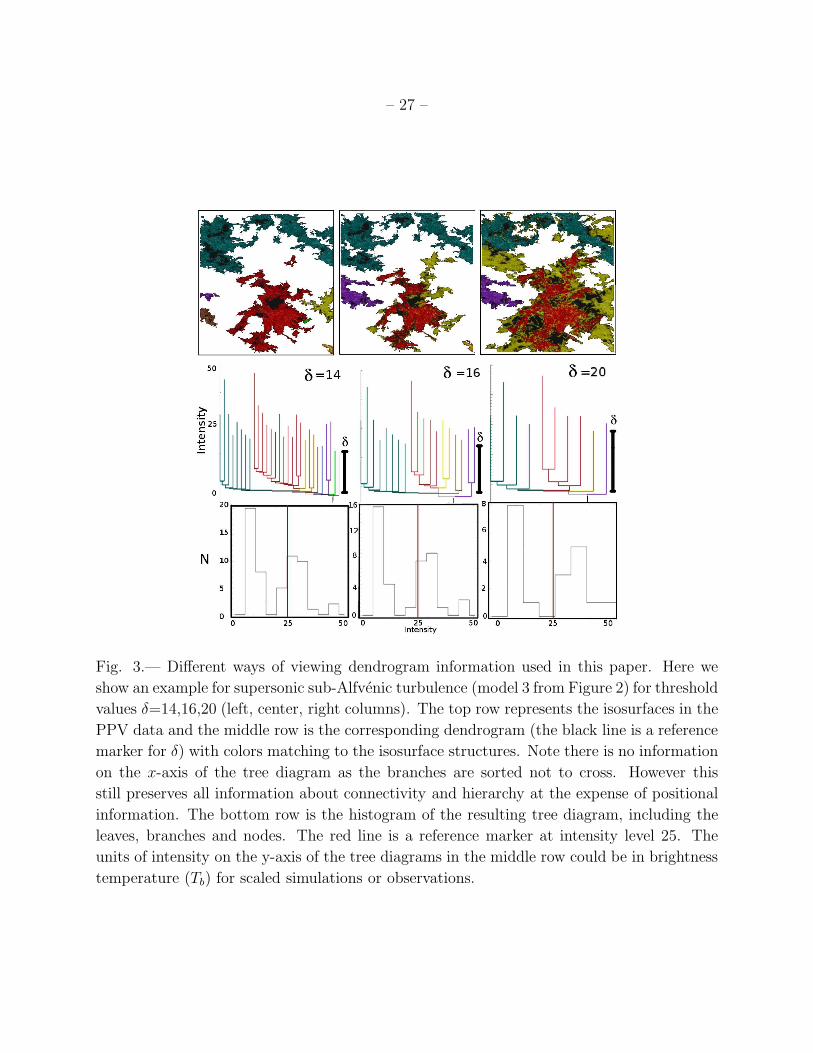
– 27 –

Fig. 3.— Different ways of viewing dendrogram information used in this paper. Here we

show an example for supersonic sub-Alfvenic turbulence (model 3 from Figure 2) for threshold

values δ=14,16,20 (left, center, right columns). The top row represents the isosurfaces in the

PPV data and the middle row is the corresponding dendrogram (the black line is a reference

marker for δ) with colors matching to the isosurface structures. Note there is no information

on the x-axis of the tree diagram as the branches are sorted not to cross. However this

still preserves all information about connectivity and hierarchy at the expense of positional

information. The bottom row is the histogram of the resulting tree diagram, including the

leaves, branches and nodes. The red line is a reference marker at intensity level 25. The

units of intensity on the y-axis of the tree diagrams in the middle row could be in brightness

temperature (Tb) for scaled simulations or observations.

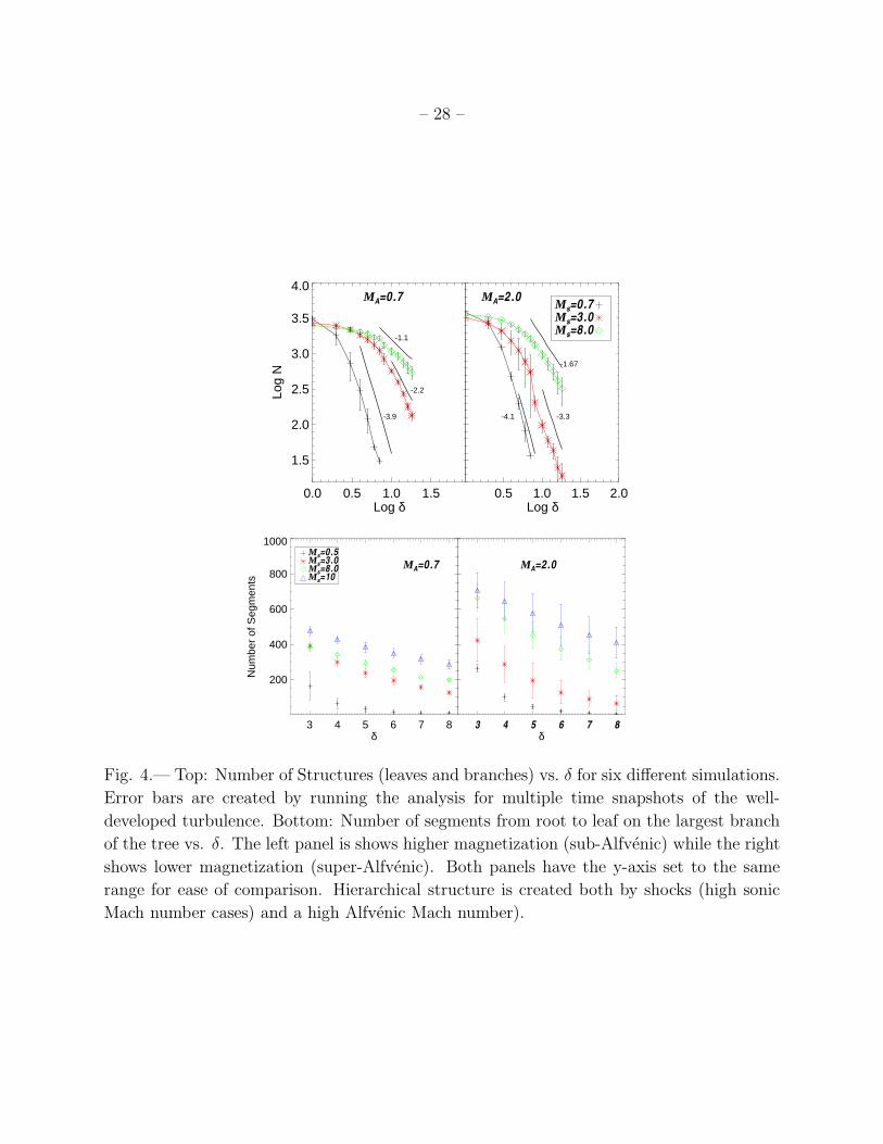
– 28 –

0.0 0.5 1.0 1.5Log δ

1.5

2.0

2.5

3.0

3.5

4.0Lo

g N

-3.9

-2.2

-1.1

0.5 1.0 1.5 2.0Log δ

-4.1 -3.3

-1.67

Ms=0.7Ms=3.0Ms=8.0

MA=0.7 MA=2.0

3 4 5 6 7 8δ

200

400

600

800

1000

Num

ber

of S

egm

ents

Ms=0.5Ms=3.0Ms=8.0Ms=10

3 4 5 6 7 8δ

MA=2.0MA=0.7

Fig. 4.— Top: Number of Structures (leaves and branches) vs. δ for six different simulations.

Error bars are created by running the analysis for multiple time snapshots of the well-

developed turbulence. Bottom: Number of segments from root to leaf on the largest branch

of the tree vs. δ. The left panel is shows higher magnetization (sub-Alfvenic) while the right

shows lower magnetization (super-Alfvenic). Both panels have the y-axis set to the same

range for ease of comparison. Hierarchical structure is created both by shocks (high sonic

Mach number cases) and a high Alfvenic Mach number).

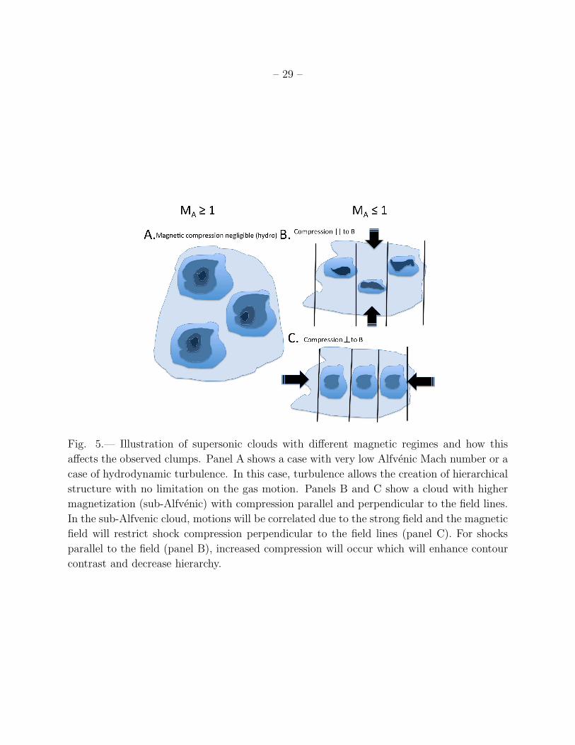
– 29 –

Fig. 5.— Illustration of supersonic clouds with different magnetic regimes and how this

affects the observed clumps. Panel A shows a case with very low Alfvenic Mach number or a

case of hydrodynamic turbulence. In this case, turbulence allows the creation of hierarchical

structure with no limitation on the gas motion. Panels B and C show a cloud with higher

magnetization (sub-Alfvenic) with compression parallel and perpendicular to the field lines.

In the sub-Alfvenic cloud, motions will be correlated due to the strong field and the magnetic

field will restrict shock compression perpendicular to the field lines (panel C). For shocks

parallel to the field (panel B), increased compression will occur which will enhance contour

contrast and decrease hierarchy.

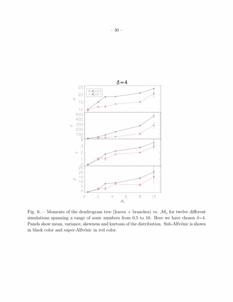
– 30 –

Fig. 6.— Moments of the dendrogram tree (leaves + branches) vs. Ms for twelve different

simulations spanning a range of sonic numbers from 0.5 to 10. Here we have chosen δ=4.

Panels show mean, variance, skewness and kurtosis of the distribution. Sub-Alfvenic is shown

in black color and super-Alfvenic in red color.

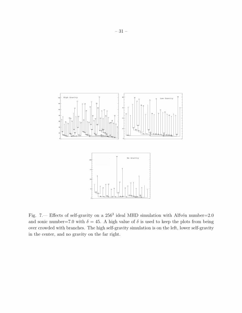
– 31 –

Fig. 7.— Effects of self-gravity on a 2563 ideal MHD simulation with Alfven number=2.0

and sonic number=7.0 with δ = 45. A high value of δ is used to keep the plots from being

over crowded with branches. The high self-gravity simulation is on the left, lower self-gravity

in the center, and no gravity on the far right.

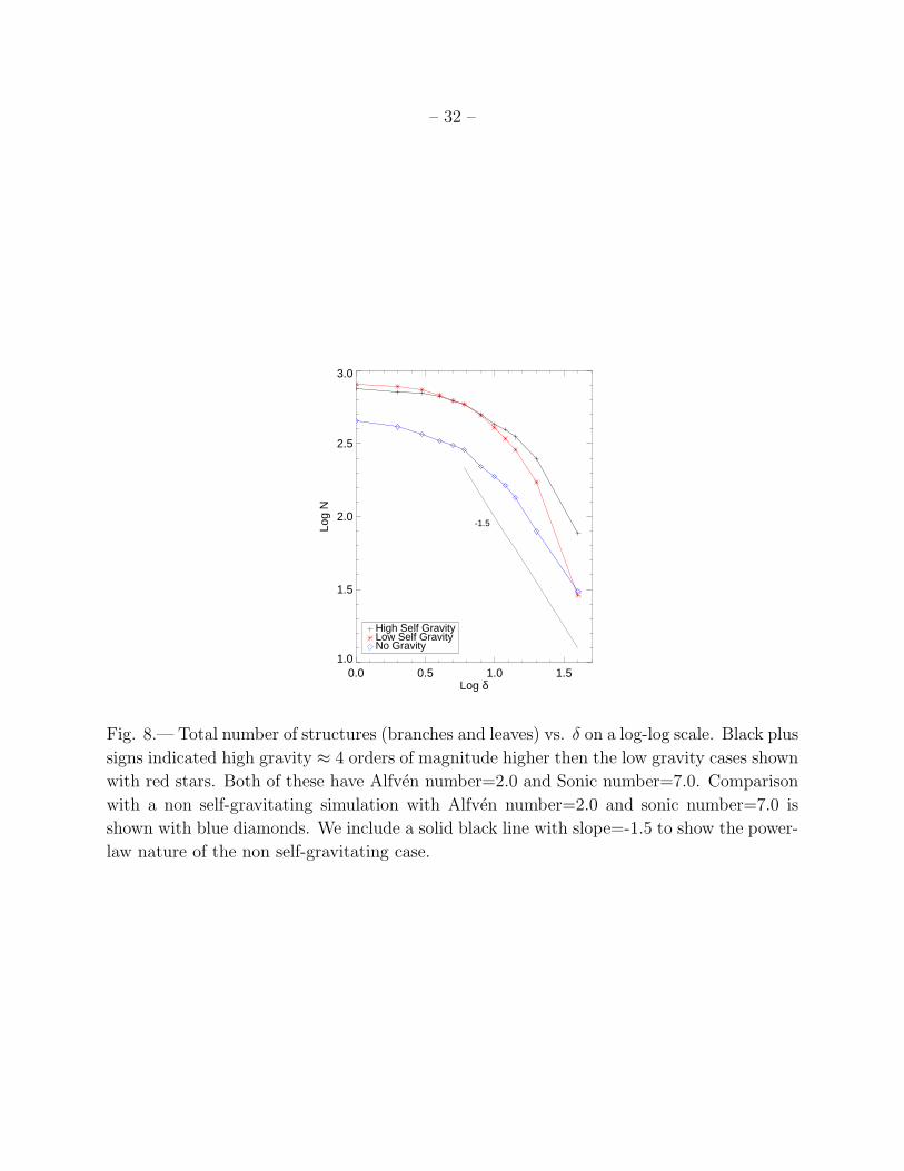
– 32 –

0.0 0.5 1.0 1.5Log δ

1.0

1.5

2.0

2.5

3.0

Log

N

No GravityLow Self GravityHigh Self Gravity

-1.5

Fig. 8.— Total number of structures (branches and leaves) vs. δ on a log-log scale. Black plus

signs indicated high gravity ≈ 4 orders of magnitude higher then the low gravity cases shown

with red stars. Both of these have Alfven number=2.0 and Sonic number=7.0. Comparison

with a non self-gravitating simulation with Alfven number=2.0 and sonic number=7.0 is

shown with blue diamonds. We include a solid black line with slope=-1.5 to show the power-

law nature of the non self-gravitating case.

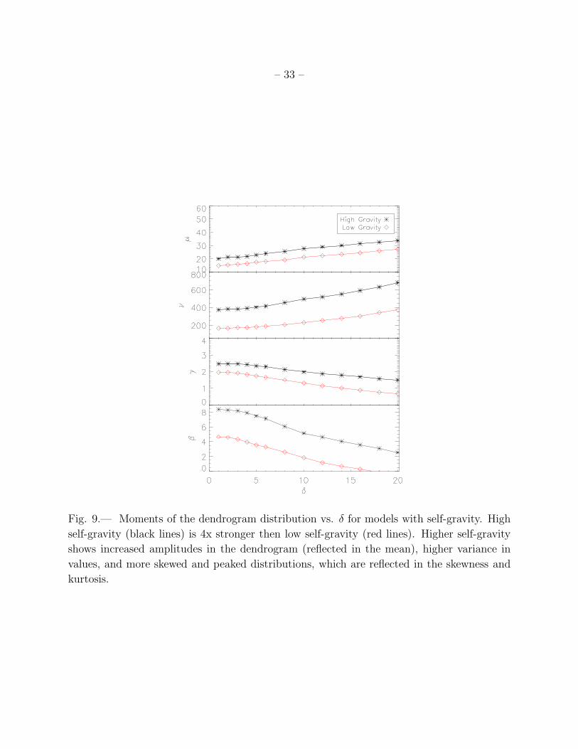
– 33 –

Fig. 9.— Moments of the dendrogram distribution vs. δ for models with self-gravity. High

self-gravity (black lines) is 4x stronger then low self-gravity (red lines). Higher self-gravity

shows increased amplitudes in the dendrogram (reflected in the mean), higher variance in

values, and more skewed and peaked distributions, which are reflected in the skewness and

kurtosis.

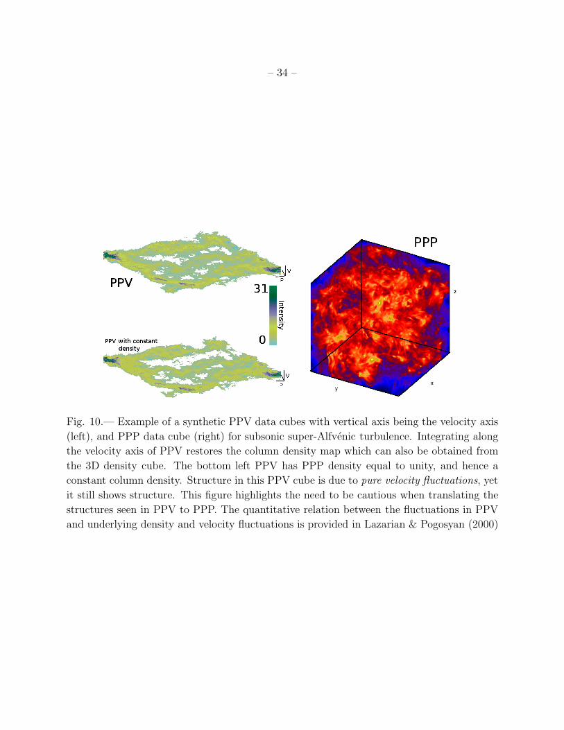
– 34 –

Fig. 10.— Example of a synthetic PPV data cubes with vertical axis being the velocity axis

(left), and PPP data cube (right) for subsonic super-Alfvenic turbulence. Integrating along

the velocity axis of PPV restores the column density map which can also be obtained from

the 3D density cube. The bottom left PPV has PPP density equal to unity, and hence a

constant column density. Structure in this PPV cube is due to pure velocity fluctuations, yet

it still shows structure. This figure highlights the need to be cautious when translating the

structures seen in PPV to PPP. The quantitative relation between the fluctuations in PPV

and underlying density and velocity fluctuations is provided in Lazarian & Pogosyan (2000)

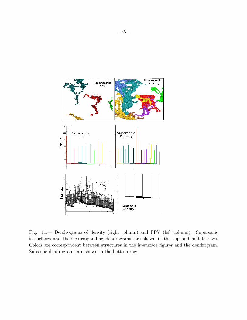
– 35 –

Fig. 11.— Dendrograms of density (right column) and PPV (left column). Supersonic

isosurfaces and their corresponding dendrograms are shown in the top and middle rows.

Colors are correspondent between structures in the isosurface figures and the dendrogram.

Subsonic dendrograms are shown in the bottom row.

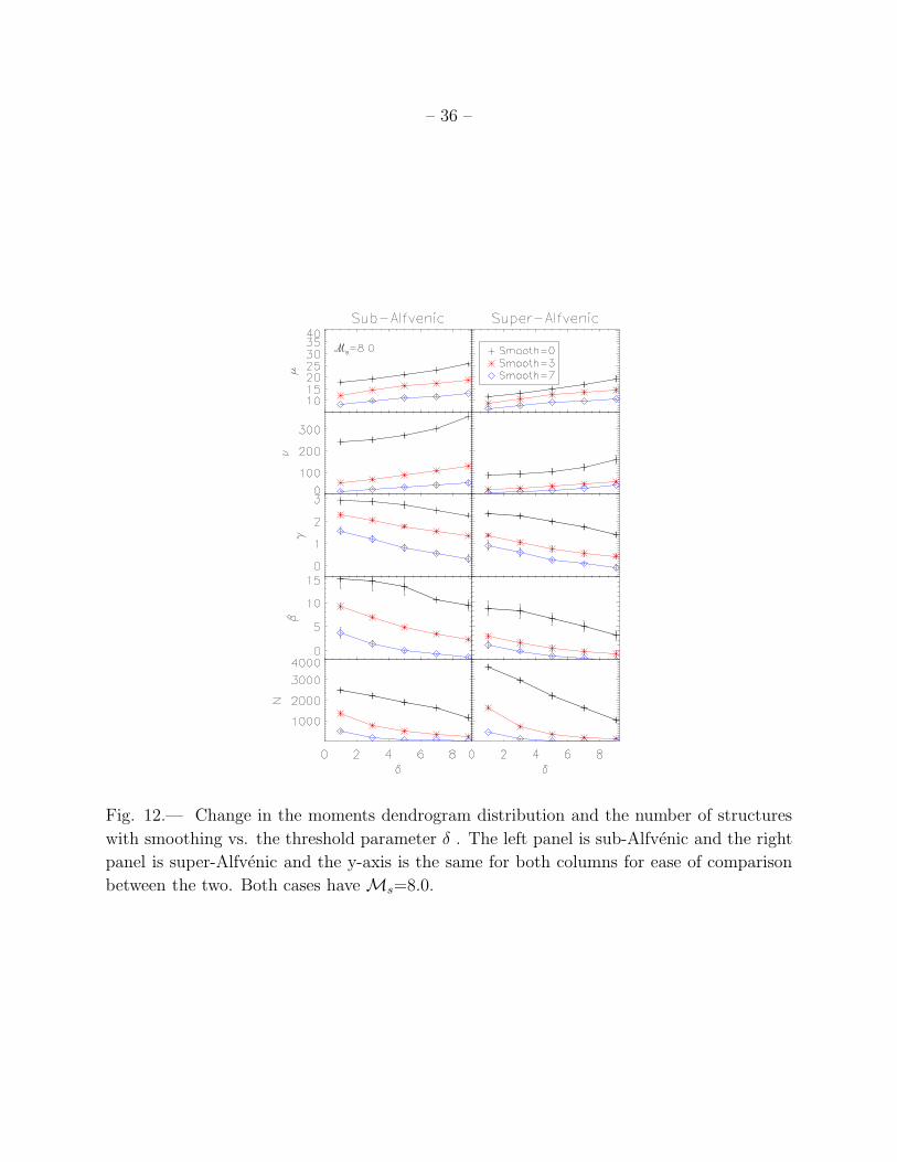
– 36 –

Fig. 12.— Change in the moments dendrogram distribution and the number of structures

with smoothing vs. the threshold parameter δ . The left panel is sub-Alfvenic and the right

panel is super-Alfvenic and the y-axis is the same for both columns for ease of comparison

between the two. Both cases have Ms=8.0.

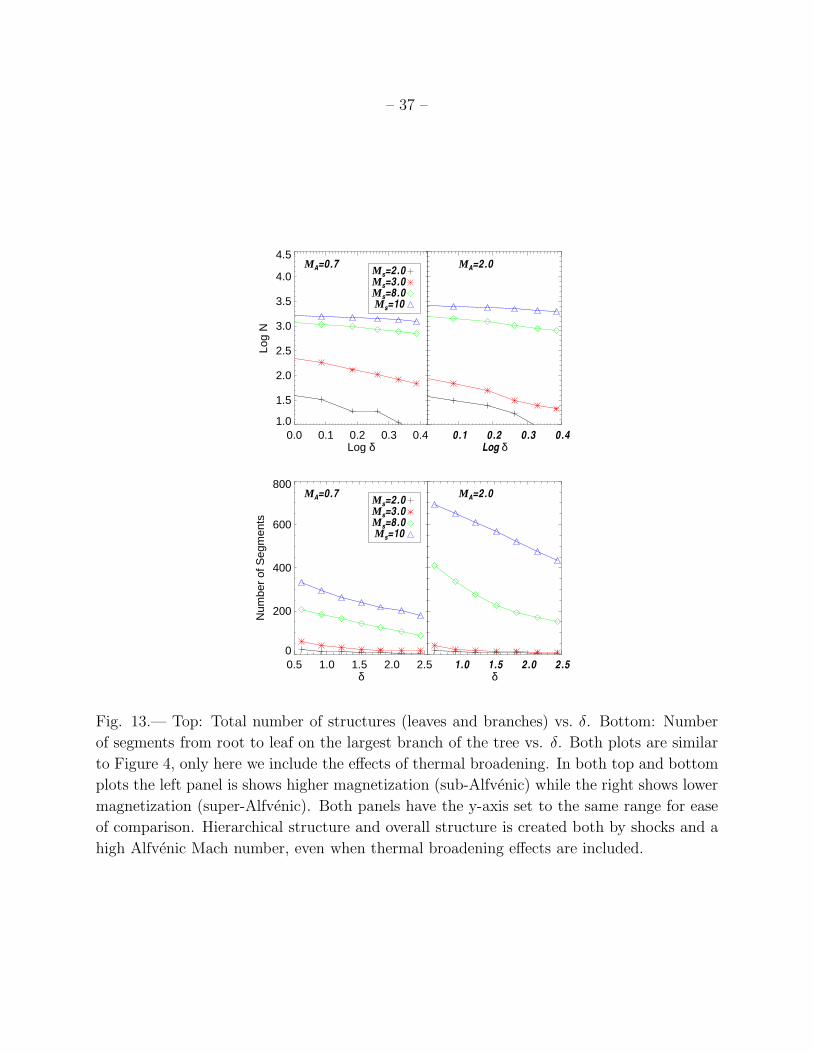
– 37 –

0.0 0.1 0.2 0.3 0.4Log δ

1.0

1.5

2.0

2.5

3.0

3.5

4.0

4.5Lo

g N

Ms=2.0Ms=3.0Ms=8.0Ms=10

0.1 0.2 0.3 0.4Log δ

MA=0.7 MA=2.0

0.5 1.0 1.5 2.0 2.5δ

0

200

400

600

800

Num

ber

of S

egm

ents

Ms=2.0Ms=3.0Ms=8.0Ms=10

1.0 1.5 2.0 2.5δ

MA=0.7 MA=2.0

Fig. 13.— Top: Total number of structures (leaves and branches) vs. δ. Bottom: Number

of segments from root to leaf on the largest branch of the tree vs. δ. Both plots are similar

to Figure 4, only here we include the effects of thermal broadening. In both top and bottom

plots the left panel is shows higher magnetization (sub-Alfvenic) while the right shows lower

magnetization (super-Alfvenic). Both panels have the y-axis set to the same range for ease

of comparison. Hierarchical structure and overall structure is created both by shocks and a

high Alfvenic Mach number, even when thermal broadening effects are included.