arX

iv:h

ep-p

h/04

0920

7v1

16

Sep

2004

Higgs Phenomenology in the

Two Higgs Doublet Model of type II

A dissertation submitted to

the University of San Francisco-Quito

in partial fulfillment of

the requirements for the degree of

Doctor of Philosophy

ByCarlos A. Marın

20 July 2004

Supervisor: Dr. Bruce Hoeneisen

Contents

1 Introduction 1

2 Limits on the Two Higgs Doublet Model from meson decay, mixing and CP violation 5

2.1 Introduction . . . . . . . . . . . . . . . . . . . . . . . . . . . . 12.2 Feynman rules of the charged Higgs in the Two Higgs Doublet Model. 22.3 Theory . . . . . . . . . . . . . . . . . . . . . . . . . . . . . . . 22.4 Limits . . . . . . . . . . . . . . . . . . . . . . . . . . . . . . . 52.5 Conclusions . . . . . . . . . . . . . . . . . . . . . . . . . . . . 5

3 Mass constraints, production cross sections, and decay rates in the Two Higgs Doublet Model of type II 10

3.1 Introduction . . . . . . . . . . . . . . . . . . . . . . . . . . . . 13.2 Masses . . . . . . . . . . . . . . . . . . . . . . . . . . . . . . . 13.3 Feynman rules . . . . . . . . . . . . . . . . . . . . . . . . . . . 43.4 Decay rates of h0 . . . . . . . . . . . . . . . . . . . . . . . . . 83.5 Branching fractions of h0 . . . . . . . . . . . . . . . . . . . . . 93.6 Decay rates of H± . . . . . . . . . . . . . . . . . . . . . . . . 103.7 Decays of H0. . . . . . . . . . . . . . . . . . . . . . . . . . . . 113.8 Decay rates of A0 . . . . . . . . . . . . . . . . . . . . . . . . . 133.9 Decay Z → h0γ . . . . . . . . . . . . . . . . . . . . . . . . . . 223.10 Vertex with four particles . . . . . . . . . . . . . . . . . . . . 233.11 Production of h0, H0 and A0 . . . . . . . . . . . . . . . . . . . 233.12 Production of h0Z0X . . . . . . . . . . . . . . . . . . . . . . . 253.13 Production of H+ . . . . . . . . . . . . . . . . . . . . . . . . . 273.14 Production of h0W+X . . . . . . . . . . . . . . . . . . . . . . 293.15 Numerical examples . . . . . . . . . . . . . . . . . . . . . . . . 313.16 Running coupling constants and GrandUnification . . . . . . . 333.17 Conclusions . . . . . . . . . . . . . . . . . . . . . . . . . . . . 35

4 Higgs production at a muon collider in the Two Higgs Doublet Model of type II 38

4.1 Introduction . . . . . . . . . . . . . . . . . . . . . . . . . . . . 14.2 Higgs bosons masses and radiative corrections . . . . . . . . . 2

i

4.3 Production of h0 , H0 . . . . . . . . . . . . . . . . . . . . . . . 54.4 Production of A0 . . . . . . . . . . . . . . . . . . . . . . . . . 114.5 Production of H± . . . . . . . . . . . . . . . . . . . . . . . . . 144.6 Production of charged Higgs boson pairs . . . . . . . . . . . . 164.7 µ−µ+ → tt annihilation . . . . . . . . . . . . . . . . . . . . . . 204.8 H∓W± production at a Hadron Collider . . . . . . . . . . . . 22

4.8.1 qq → H−W+ interaction . . . . . . . . . . . . . . . . . 224.8.2 gg → H−W+ interaction . . . . . . . . . . . . . . . . 254.8.3 Differential cross section pp→ H∓W±X . . . . . . . . 26

4.9 Comparison between µ−µ+ → H∓W± and pp, pp→ H∓W±X for large values of tan β 304.10 Conclusions . . . . . . . . . . . . . . . . . . . . . . . . . . . . 31

A Functions SWW , SHW and SHH 1

B Calculation of the box diagrams corresponding to charged Higgs contributions to B0 − B0 mixing in the “Two Higgs Doublet Model of type II” 3

B.1 Invariant amplitude MHH . . . . . . . . . . . . . . . . . . . . 3B.2 Invariant amplitude MHW . . . . . . . . . . . . . . . . . . . . 7B.3 Invariant amplitude MWW . . . . . . . . . . . . . . . . . . . . 10B.4 Mass difference ∆mB . . . . . . . . . . . . . . . . . . . . . . . 11

C Integrals 12

C.1 IHHα (i, j) . . . . . . . . . . . . . . . . . . . . . . . . . . . . . . 12

C.2(

IHWα

)(1)(i, j) . . . . . . . . . . . . . . . . . . . . . . . . . . . 13

C.3(

IHWα

)(2)(i, j) . . . . . . . . . . . . . . . . . . . . . . . . . . . 13

C.4 IHW (i, j) . . . . . . . . . . . . . . . . . . . . . . . . . . . . . . 14C.5 IHW

αβ (i, j) . . . . . . . . . . . . . . . . . . . . . . . . . . . . . . 14

D A0 → Z0γ decay 16

D.1 (a) i = e−, µ−, τ−, d, s, b . . . . . . . . . . . . . . . . . . . . . 16D.2 b) i = u, c, t . . . . . . . . . . . . . . . . . . . . . . . . . . . . 21D.3 Width decay . . . . . . . . . . . . . . . . . . . . . . . . . . . . 21

ii

Chapter 1

Introduction

The Standard Model of quarks and leptons is based on some basic principles:special relativity, locality, quantum mechanics, local symmetries and renor-malizability [1]. Therefore the predictions of the Standard Model “are preciseand unambiguous, and generally cannot be modified ‘a little bit’ except invery limited specific ways. This feature makes the experimental success espe-cially meaningful, since it becomes hard to imagine that the theory could beapproximately right without in some sense being exactly right.”[1] The Stan-dard Model predicts the existence of a massive spin zero boson called Higgsparticle. The Higgs mechanism is responsible for the masses of the weakinteraction gauge bosons W± and Z0, and is also sufficient to give masses tothe leptons and quarks. The discovey of the Standard Model Higgs is thenone of the principal goals of experimental and theoretical particle physicists.We could say that the Higgs mechanism is a cornerstone of the StandardModel.

Among the extensions of the Standard Model that respect its principlesand symmetries, that are compatible with present data within a region ofparameter space, and are of interest at the large particle colliders, is the ad-dition of a second doublet of Higgs fields. Higgs doublets can be added to theStandard Model without upsetting the Z/W mass ratio; higher dimensionalrepresentations upset this ratio [2].

In the Two Higgs Doublet Model there are two choices for the Higgs-quarkinteractions. In Model I, the quarks and leptons do not couple to the firstHiggs doublet (Φ1), but couple to the second Higgs doublet (Φ2). In ModelII, Φ1 couples only to down-type quarks and leptons and Φ2 couples onlyto up-type quarks and neutrinos. If we consider the neutrinos as masslessparticles, there are no couplings between neutrinos and neutral Higgs bosons.The Model II choice for the Higgs-fermion couplings is the required structurefor the Minimal Supersymmetric Model.

1

After the electroweak symmetry-breaking mechanism, three of the eightdegrees of freedom are absorbed by the W± and Z0 gauge bosons, leadingto the existence of five elementary Higgs particles. The physical spectrumof the Two Higgs Doublet Model (Model II) contains five Higgs bosons:one pseudoscalar A0 (CP-odd scalar), two neutral scalars H0 and h0 (CP-even scalars), and two charged scalars H+ and H−. In the most generalmodel, the masses of the Higgs bosons, the mixing angle α (−π/2 < α ≤ 0)between the two neutral scalar Higgs fields, and the ratio of the vacuumexpectation values of the two neutral components of the Higgs doublets, tan β(0 ≤ β < π

2), are all independent parameters of the theory [3]. However, in

the Minimal Supersymmetric Model the conditions on the potential imposedby supersymmetry reduces the number of parameteres to two, which may bechosen to be tanβ and mH [3].

Φ1 =

(

Φo∗1

−Φ−1

)

, Φ2 =

(

Φ+2

Φo2

)

, tan β ≡ 〈Φo2〉

〈Φo∗1 〉.

In this thesis we study the Two Higgs Doublet Model of type II, set limitsto the parameter tan β as a function of the mass of the charged Higgs mH ,and find interesting discovery channels in hadron colliders or muon colliders.

All the analysis in this thesis are based on the “tree-level Higgs potential”[3].

The plan in my thesis is the following:In the second Chapter[4], using the experimental data on meson decay

rates, mixing and CP violation in the K0 and B0 systems, we set limits tothe parameter tanβ as a function of the mass of the charged Higgs mH .Recent measurements of sin(2βCKM) by the B-factories Belle [5] and BaBar[6] permit us to set more stringent limits on tan β. βCKM is an angle of the“unitarity triangle”. [7]

In the third Chapter[8], we present graphically the corresponding lim-its on mH0 , mh0 and mA0 as a function of the mass of the charged Higgs,without considering the influence of radiative corrections. Then we calcu-late production cross sections, decay rates and branching fractions of theHiggs particles. Next, we obtain the running coupling constants and discussGrand Unification. Finally, in the Conclusions, we list interesting discoverychannels.

In Chapter four [9], we analyze the possibility of the construction ofa µ−µ+ collider to detect charged or neutral Higgs bosons. The reasonfor this is that in a muon collider, the signal could be cleaner than ina hadron collider. Some of the production cross sections that we studyare: µ−µ+ → h0Z0, H0Z0, H−H+, A0Z0 and H∓W±. Then, we compare

2

the channel µ−µ+ → H∓W± (at√s = 500GeV/c and for large values of

tan β) with the production processes pp → H∓W±X (at the Tevatron) andpp → H∓W±X (at the LHC), taking into account the tt background, tocheck the feasibility of detecting H± using a muon collider. The influenceof radiative corrections in the masses of the Higgs bosons is considered inall the calculations. Finally, in the Conclusions, we also check the processµ−µ+ → A0h0.NOTE : The results presented in this thesis (width decays, production crosssections, etc.) are calculated in detail in reference [10].

3

Bibliography

[1] Frank Wilczek, “Beyond the Standard Model: an answer and twentyquestions”, hep-ph/9802400 (1998).

[2] Bruce Hoeneisen, Serie de Documentos USFQ 26, Universidad San Fran-cisco de Quito, Ecuador (2001).

[3] Vernon Barger and Roger Phillips, Collider Physics (Addison Wesley,1988); S. Dawson, J.F. Gunion, H.E. Haber and G. Kane, The HiggsHunter’s Guide (Addison Wesley, 1990).

[4] Carlos A. Marın and Bruce Hoeneisen, hep-ph/0210167 (2002).

[5] K. Abe et.al. (Belle Collaboration), Belle Preprint 2002-6 and hep-ex/0202027v2, 2002.

[6] B. Aubert et.al., SLAC preprint SLAC-PUB-9153, 2002 and hep-ex/0203007.

[7] 2002 Review of Particle Physics, The Particle Data Group, K. Hagiwaraet.al., Phys. Rev. D 66 (2002) 010001.

[8] C. Marın and B. Hoeneisen, hep-ph/0402061 v1 (2004).

[9] C. Marın, hep-ph/0405021 v1 (2004).

[10] C. Marın, Higgs Phenomenology in the Two Higgs Doublet Model oftype II (personal notes), Volumenes I, II and III, Universidad San Fran-cisco de Quito (2004).

4

Chapter 2

Limits on the Two Higgs

Doublet Model from meson

decay, mixing and CP violation

Abstract

We calculate the rate of π+, K+, D+ and B+ → µ+νµ decays, the branchingratio corresponding to H+ → τ+ντ , and the box diagrams of Bo ↔ Bo,Ko ↔ Ko and Do ↔ Do mixing in the Two Higgs Doublet Model (Model II).Using the experimental data on meson decay rates, mixing, and CP violationin the Ko and Bo systems we set competitive upper and lower limits to theparameter tan β as a function of the mass of the charged Higgs mH .

2.1 Introduction

The Standard Model of quarks and leptons is here to stay. This theory isbased on principles: special relativity, locality, quantum mechanics, localsymmetries and renormalizability[1]. Therefore the predictions of the Stan-dard Model “are precise and unambiguous, and generally cannot be modified‘a little bit’ except in very limited specific ways. This feature makes theexperimental success especially meaningful, since it becomes hard to imaginethat the theory could be approximately right without in some sense beingexactly right.”[1] Among the extensions of the Standard Model that respectits principles and symmetries, that are compatible with present data withina region of parameter space, and are of interest at the large particle colliders,is the addition of a second doublet of Higgs fields. Higgs doublets can beadded to the Standard Model without upsetting the Z/W mass ratio; higherdimensional representations upset this ratio. A second Higgs doublet couldmake the three running coupling constants of the Standard Model meet atthe Grand Unified Theory (GUT) scale. A second Higgs doublet is neces-sary in Supersymmetric extensions of the Standard Model[2]. In this articlewe explore the limits that present data place on the parameters of the TwoHiggs Doublet Model (Model II).[3] In particular we consider meson decay,mixing and CP violation.

All of our analysis is based on the “tree-level Higgs potential”[3]. Thephysical spectrum of the Two Higgs Doublet Model (Model II) contains fiveHiggs bosons: one pseudoscalar Ao (CP-odd scalar), two neutral scalars Ho

and ho (CP-even scalars), and two charged scalars H+ and H−. In themost general model, the masses of the Higgs bosons, the mixing angle αbetween the two neutral scalar Higgs fields, and the ratio of the vacuumexpectation values of the two neutral components of the Higgs doublets,tan β > 0, are all independent parameters of the theory. However, in theMinimal Supersymmetric Model the conditions on the potential imposed bysupersymmetry reduces the number of parameters to two, which may bechosen to be tanβ and mH [3].

Φ1 =

(

Φo∗1

−Φ−1

)

, Φ2 =

(

Φ+2

Φo2

)

, tan β ≡ 〈Φo2〉

〈Φo∗1 〉.

Using the experimental data on meson decay rates, mixing and CP violationwe set limits to the parameter tan β as a function of the mass of the chargedHiggs mH . Recent measurements of sin(2βCKM) by the B-factories Belle[5]and BaBar[6] permit us to set more stringent limits on tan β. βCKM is anangle of the “unitarity triangle”.[7]

1

2.2 Feynman rules of the charged Higgs in

the Two Higgs Doublet Model.

The effective Lagrangian corresponding to the H±f f ′ vertex is:

LH±ff ′ =g

2√2mW

H+Vff ′uf(

A+Bγ5)

vf ′

+H−V ∗ff ′ uf ′(A−Bγ5)vf (2.1)

whereA ≡ (mf ′ tan β +mfcotβ) (2.2)

andB ≡ (mf ′ tanβ −mfcotβ) , (2.3)

f = fermion (quark or lepton) and f ′ = antifermion (antiquark or antilepton).Vff ′ is an element of the CKM matrix.

The charged-Higgs propagator is: i/ (K2 −m2H + iε).

2.3 Theory

Consider the(

Bo, Bo)

system. Bo ↔ Bo mixing occurs because of the boxdiagrams illustrated in Figure 2.1. The difference in mass of the two eigen-states that diagonalize the hamiltonian can be written in the form

∆mB =βBG

2Fm

2W f

2BmB

6π2

×∣

∣

∣

∣

∣

∑

i,j

ξiξj

[

SWW − 2 cot2 β · SHW +1

4cot4 β · SHH

]

∣

∣

∣

∣

∣

. (2.4)

The functions

SWW(

xiW , xjW

)

, SHW(

xiW , xjW , x

iH , x

jH , x

WH

)

and SHH(

xiH , xjH , x

WH

)

are obtained from the box diagrams and are written in Appendix A. TheFeynman rules for H± are listed in Section 2.2. We have derived[8] SWW inagreement with the literature[9]. The derivation of SHW and SHH is givenin Appendices B and C [10]. The variables of these functions are

xiW ≡m2

i

m2W

, xiH ≡m2

i

m2H

, and xWH ≡m2

W

m2H

2

where i = u, c, t. ξi ≡ VibV∗id. The notation for the remaining symbols

in (2.4) is standard[7]. To obtain the Standard Model[9], omit SHW andSHH . βB is a factor of order 1. Estimates of βB using “vacuum intermedi-ate state insertion”[9], “PCAC and vacuum saturation”[9], “bag model”[9],“QCD corrections”[11, 12], and the “free particles in a box”[8] models spanthe range ≈ 0.4 to ≈ 1. fB is the decay constant that appears in the decayrate for B+ → µ+νµ[7] which at tree level in the Two Higgs Doublet Model(Model II) is:

ΓB+ =|Vub|28π

G2Fm

2µmB+

(

1−m2

µ

m2B+

)2 [

fB − gBm2

B+

m2H

tan2 β

]2

(2.5)

In the derivation of (2.5) we have substituted

v(

b)

γµ(

1− γ5)

u (u)→ pµfB,

v(

b) (

1− γ5)

u (u)→ −m2B+

mb

gB

which defines the decay constants fB and gB. v(

b)

and u (u) are spinors,see Section 2. We expect fB ≈ gB: for a scalar meson with the quark andantiquark at rest fB =

mB+

mbgB. The decays B+ → µ+νµ and D+ → µ+νµ

are not yet accessible to experiment so that fB and fD are unknown. fBis estimated using sum rules[13], or the B∗ − B mass difference[14], or aphenomenological model[15], or the MIT bag model[16]. These estimatesspan the range ≈ 0.06GeV to ≈ 0.2GeV with the convention used in reference[7] and in Equation (2.5).

In the “free particles in a box”[8] model βB = 1 (after correcting [8]by a color factor 4/3) and the volume of the box, i.e. the meson, is V =8/ (βBmBf

2B).

For the(

Bos , B

os

)

system: ξi ≡ VibV∗is where i = u, c, t; in (2.4) replace

subscript B by Bs. For the(

Ko, Ko)

system: ξi ≡ VisV∗id where i = u, c, t; in

(2.4) replace subscript B by K. The CP violation parameter ε[9, 7] in the(

Ko, Ko)

system in the Two Higgs Doublet Model is given by:

ε = eiπ4 ·

Im(

∑

i,j ξiξj[

SWW − 2 cot2 β · SHW + 14cot4 β · SHH

]

)

2√2 ·∣

∣

∣

∑

i,j ξiξj[

SWW − 2 cot2 β · SHW + 14cot4 β · SHH

]

∣

∣

∣

(2.6)

For the(

Do, Do)

system: ξi ≡ VciV∗ui where i = d, s, b; in (2.4) replace

subscript B by D and replace cot β by tanβ (leave tan β as is in (2.5)).The branching ratio for H+ → τ+ντ for mH < mt is given by

B(

H+ → τ+ντ)

≈ m2τ tan

2 β

|Vcs|2 a+ |Vcb|2 b+m2τ tan

2 β(2.7)

3

b− W+/-

q−

j

bW+/-q

i

b−

j q−

W+/-

biq

W+/-

b−

H+/- q−

j

bH+/-q

i

b−

j q−

H+/-

biq

H+/-

b− W+/-

q−

j

bH+/-q

i

b−

j q−

W+/-

biq

H+/-

b−

H+/- q−

j

bW+/-q

i

b−

j q−

H+/-

biq

W+/-

Figure 2.1: Feynman diagrams corresponding to Bo ↔ Bo mixing in the TwoHiggs Doublet Model. q = d or s and i, j = u, c, t. The diagrams on the rightside interfer with a “-” sign.

4

with a ≡ 3 [m2s tan

2 β +m2c cot

2 β] and b ≡ 3 [m2b tan

2 β +m2c cot

2 β]. Fromthe measured limit[17] on mH as a function of the branching ratio and (2.7)we obtain a lower bound of mH for each tanβ.

Let us finally mention that the time-dependent CP-violating asymmetryA ≡ (Γ − Γ)/(Γ + Γ), where Γ (Γ) is the rate of the decay Bo → J/ψ +Ks (Bo → J/ψ + Ks), measured by CDF, Belle and BaBar is given bysin(2βCKM) · sin(∆Mt) in both the Standard Model and in the Two HiggsDoublet Model (Model II). This is because the dominating terms of ξiξjS

HW

and ξiξjSHH have i = j = t.

2.4 Limits

All experimental data are taken from [7]. In order to obtain limits we assumeconservatively 0.4 < βx < 1.8, and fx = gx with x = B, Bs, D, K, π. Theseassumptions are not critical since the upper (lower) limits on tanβ dependon terms ∝ tan4 β (∝ cot4 β) in (2.4) or (2.5). We take the magnitude ofthe elements of the CKM matrix from [7] and leave the phase ∠Vub as afree parameter. The following calculations are made for each (mH , tan β).The measured value of the parameter ε determines the phase ∠Vub of theCKM matrix, and hence βCKM . This phase is required to be within theexperimental bounds: 0.325 < tan(βCKM) < 0.862 at 95% confidence level[7]. The measured decay rates ΓK and Γπ determine fK and fπ using (2.5).The experimental upper bounds on ΓB and ΓD determine upper bounds onfB and fD using (2.5). The measured ∆mB and ∆mK determine βBf

2B and

βKf2K using (2.4). The experimental upper bound on ∆mD determines an

upper bound on βDf2D. The experimental lower bound on ∆mBs determines

a lower bound on βBsf2Bs. From the preceding information we obtain βK and

a lower bound on βB. Then the requirements 0.4 < βK < 1.8, βB < 1.8and 0.325 < tan(βCKM) < 0.862 place limits on tan β for each mH as listedin Table 2.1. The confidence level of these limits is 95%. It turns out thatthe lower limit on tanβ is determined by the experimental lower limit oftan(βCKM), and the upper limit on tan β is determined by βB < 1.8.

2.5 Conclusions

Using measured meson decay rates, mixing and CP violation we have ob-tained lower and upper bounds of tanβ for each mH . These limits are com-pared with the results of direct searches in Figures 2.2. Note that the mea-surements of sin(2βCKM) by the Belle and BaBar collaborations have raised

5

mH = 100GeV 1.74 < tanβ < 67mH = 200GeV 1.36 < tanβ < 134mH = 300GeV 1.13 < tanβ < 202mH = 1000GeV 0.58 < tanβ < 672

Table 2.1: Limits on tanβ for severalmH from measurements of meson decay,mixing and CP violation. These limits correspond to 95% confidence.

0.1 1 10 100 10000

100

200

300

tan(beta)

mH

(GeV/c )2

LEP2

CDFCDF

D0 D0

excludedby this work excluded

by this work

excluded by

allowedregion

Figure 2.2: Lower and upper limits on tanβ as a function of the mass of thecharged Higgs mH from meson decay, mixing and CP violation (continuouscurve) compared to limits obtained by CDF[18], D0[19] and LEP2[20], all at95% confidence.

6

the lower bound on tanβ by a factor ≈ 5 with respect to our previous cal-culation [4]. It is important to mention that an indirect limit by the CLEOcollaboration [21] obtained from the measurements of the b→ sγ transition,limits the Two Higgs Doublet Model of type II to have a charged Higgs massin excess of about 264GeV/c2 (it is a slow function of tan β).

7

Bibliography

[1] Frank Wilczek, “Beyond the Standard Model: an answer and twentyquestions”, hep-ph/9802400 (1998) .

[2] R.D. Peccei, “Physics beyond the Standard Model”, hep-ph/9909233(1999).

[3] Vernon Barger and Roger Phillips, Collider Physics (Addison Wesley,1988), pages 452-454; S. Dawson, J. F. Gunion, H.E. Haber and G.Kane, The Higgs Hunter’s Guide (Addison Wesley, 1990), p. 383.

[4] Carlos A. Marın and Bruce Hoeneisen, Revista Colombiana de Fısica,31, No. 1, 34 (1999).

[5] K. Abe et.al. (Belle Collaboration), Belle Preprint 2002-6 and hep-ex/0202027v2, 2002.

[6] B. Aubert et.al., SLAC preprint SLAC-PUB-9153, 2002 and hep-ex/0203007.

[7] 2002 Review of Particle Physics, The Particle Data Group, K. Hagiwaraet.al., Phys. Rev. D 66 (2002) 010001.

[8] Carlos Marın and Bruce Hoeneisen, POLITECNICA XVI, No. 2, 33(1991), Escuela Politecnica Nacional, Quito, Ecuador.

[9] Ling-Lie Chau, Physics Reports 95, No. 1, 1 (1983).

[10] Carlos Marın and Bruce Hoeneisen, Serie Documentos USFQ No. 15(1996), Universidad San Francisco de Quito.

[11] Yosef Nir, Nucl. Phys. B306, 14 (1988).

[12] A. J. Buras, M. Jamin and P. H. Weisz, Nucl. Phys. B347, 491 (1990).

[13] L. J. Reinders, Phys. Rev. D 38, 947 (1988).

8

[14] M. Suzuki, Phys. Lett. 162B, 392 (1985).

[15] M. Suzuki, Nucl. Phys. B177, 413 (1981); Phys. Lett. 142B, 207 (1984).

[16] E. Golowich, Phys. Lett. 91B, 271 (1980); M. Claudson, Hardvard Uni-versity preprint HUTP-81/A016.

[17] A. Heister et. al. (ALEPH), hep-ex/0207054 v1 (2002).

[18] CDF Collab., Phys. Rev. Lett. 79, 357 (1997).

[19] D0 Collab., Phys. Rev. Lett. 82, 4975 (1999); FERMILAB-Conf-00-294-E.

[20] LEP Higgs Working Group, http://lephiggs.web.cern.ch/LEPHIGGS/papers/index.html; LHWG Note/2001-05.

[21] M. S. Alam et al., Phys. Rev. Lett. 74, 2885 (1995).

9

Chapter 3

Mass constraints, production

cross sections, and decay rates

in the Two Higgs Doublet

Model of type II

Abstract

We calculate masses, production cross sections, and decay rates in the TwoHiggs Doublet Model of type II. We also discuss running coupling con-stants and Grand Unification. The most interesting production channelsare gg → h0, H0, A0 on mass shell, and qq, gg → h0Z and qq′ → h0W± inthe continuum (tho there may be peaks at mA0). The most interesting de-cays are h0, H0, A0 → bb-jets and τ+τ−, and, if above threshold, H0 → ZZ,W+W− and h0h0. The following final states should be compared with theStandard Model cross section: bbZ, bbW±, τ+τ−Z, τ+τ−W±, bb, τ+τ−, ZZ,W+W−, 3 and 4 b-jets, 2τ++2τ−, bbτ+τ−, ZW+W−, 3Z, ZZW± and 3W±.Mass peaks should be searched in the following channels: Zbb, ZZ, ZZZ,bb, 4b-jets and, just in case, Zγ.

3.1 Introduction

Among the extensions of the Standard Model that respect its principles andsymmetries, and are compatible with present data within a region of param-eter space, and are of interest at the large particle colliders, is the additionof a second doublet of Higgs fields. In this article we consider the Two HiggsDoublet Model of type II[1]. The Higgs sector of the Minimal Supersymmet-ric Standard Model (MSSM) is of this type (tho the model of type II does notrequire Supersymmetry). The physical spectrum of the model contains fiveHiggs bosons: one pseudoscalar Ao (CP-odd scalar), two neutral scalars Ho

and ho (CP-even scalars), and two charged scalars H+ and H−. The massesof the charged Higgs bosons mH , and the ratio of the vacuum expectationvalues of the two neutral components of the Higgs doublets, tanβ > 0, arefree parameters of the theory.

In [2] we obtained limits in the (mH , tanβ) plane using measured de-cay rates, mixing and CP violation of mesons. In this article we presentgraphically the corresponding limits on mH0 , mh0 and mA0. Then we cal-culate production cross sections, decay rates and branching fractions of theHiggs particles. Next, we obtain the running coupling constants and discussGrand Unification. Finally, in the Conclusions, we list interesting discoverychannels.

3.2 Masses

The masses of the neutral Higgs particles as a function of the masses of thecharged HiggsmH , tanβ and the masses of Z andW , calculated at tree level,are:

m2A0 = m2

H −m2W , (3.1)

2m2H0 = m2

H −m2W +m2

Z

+

[

(

m2H −m2

W +m2Z

)2 − 4m2Z

(

m2H −m2

W

)

(

tan2 β − 1

tan2 β + 1

)2]

1

2

(3.2)

2m2h0 = m2

H −m2W +m2

Z

−[

(

m2H −m2

W +m2Z

)2 − 4m2Z

(

m2H −m2

W

)

(

tan2 β − 1

tan2 β + 1

)2]

1

2

(3.3)

1

0.1 1 10 100 10000

100

200

300

tan(beta)

mH

(GeV/c )2

LEP2

CDFCDF

D0 D0

excludedby this work excluded

by this work

excluded by

allowedregion

Figure 3.1: Lower and upper limits on tanβ as a function of the mass of thecharged Higgs mH from meson decay, mixing and CP violation (continuouscurve) compared to limits obtained by CDF[3], D0[4] and LEP2[5], all at95% confidence. Taken from [2].

We have re derived these equations in agreement with the literature.[1]In Chapter two [2] we obtained the limits in the (tanβ,mH) plane shown

in Figure 3.1. From that figure and Equations 3.1, 3.2 and 3.3 we obtain thelimits on the masses of the neutral Higgs particles shown in Figure 3.2.

Radiative corrections can be very large. In the MSSM the largest contri-butions arise from the incomplete cancellation between top and stop loops.The corresponding plot similar to Figure 3.2 with radiative corrections canbe found in [6].

2

[GeV/c ]2

[GeV/c ]2

600

500

400

300

200

100

00 100 200 300 400

H+m

Allowed region for mh0

Allowed region for mH

0

mA

0

Figure 3.2: Allowed regions of the masses of the neutral Higgs h0, H0 andA0 as a function of the mass mH of the charged Higgs H±. From Figure 3.1and the tree level Equations 3.1, 3.2 and 3.3. Radiative corrections raise theallowed region of h0.[6]

3

3.3 Feynman rules

The Lagrangian for the V HH interaction is:[1]

LV HH =−ig2W+

µ ·H−←→∂ µ[

H0 sin(α− β) + h0 cos(α− β) + iA0]

+ h.c.

− ig

2 cos θWZµiA0←→∂ µ

[

H0 sin(α− β) + h0 cos(α− β)]

−(

2 sin2 θW − 1)

·H−←→∂ µH+ (3.4)

whereA←→∂ µB = A(∂µB)− (∂µA)B. (3.5)

The Lagrangian for the V V H interaction is:

LV V H =

(

gmWW+µ W

−µ +gmZ

2 cos θWZµZ

µ

)

×[

H0 cos(β − α) + h0 sin(β − α)]

. (3.6)

There are no vertices ZH0H0, Zh0h0, ZA0A0, ZW+H− or ZH0h0. Theinteractions of neutral Higgs bosons with up and down quarks are given by:

LAHhff ′ =−gmf

2mW sin β

[

ufvf (H0 sinα + h0 cosα)− i cos β · ufγ5vfA0

]

− gmf ′

2mW cos β

×[

uf ′vf ′(H0 cosα− h0 sinα)− i sin β · uf ′γ5vf ′A0]

(3.7)

where f = u, c, t, νe, νµ, ντ and f ′ = d, s, b, e−, µ−, τ−. The Lagrangian corre-sponding to the H±f f ′ vertex is:

LH±ff ′ =g

2√2mW

H+Vff ′uf(

A+Bγ5)

vf ′

+H−V ∗ff ′ uf ′(A−Bγ5)vf (3.8)

where A ≡ (mf ′ tanβ +mf cot β) and B ≡ (mf ′ tan β −mf cot β). Vff ′ is anelement of the CKM matrix. The Lagrangian corresponding to three Higgs

4

bosons is:

L3h = −gH0H+H−[

mW cos(β − α)− mZ

2 cos θWcos(2β) cos(β + α)

]

+mZ

4 cos θWH0H0 cos(2α) cos(β + α)

+mZ

4 cos θWh0h0 [2 sin(2α) sin(β + α)− cos(β + α) cos(2α)]

− mZ

4 cos θWA0A0 cos(2β) cos(β + α)

−gh0H+H−[

mW sin(β − α) + mZ

2 cos θWcos(2β) sin(β + α)

]

+mZ

4 cos θWh0h0 cos(2α) sin(β + α)

− mZ

4 cos θWH0H0 [2 sin(2α) cos(β + α) + sin(β + α) cos(2α)]

+mZ

4 cos θWA0A0 cos(2β) sin(β + α). (3.9)

Vertexes with four partons including two Higgs bosons are

L4 = e2AµAµH+H− +

eg cos (2θW )

cos θWAµZ

µH+H−

−eg2sin (β − α)AµW

±µH0H∓ +eg

2cos (β − α)AµW

±µh0H∓

±ige2AµW

±µA0H∓, (3.10)

The H+H−γ vertex is

LH+H−γ = −ig sin θWAµH−←→∂µH+ (3.11)

The Higgs propagators are: i/ (k2 −m2 + iε).Feynman diagrams corresponding to the production of Zh0 are shown in

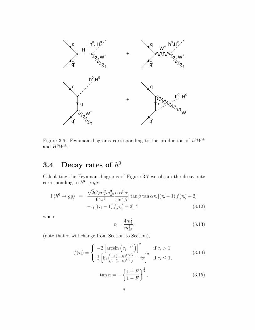
Figures 3.3, 3.4 and 3.5. Note that the invariant mass of Zh0 can have aresonance at mA0 which is an interesting experimental signature. Feynmandiagrams corresponding to the production of W±h0 or W±H0 are shown inFigure 3.6.

5

q

q−

A0h0

Z0 +

q

q−

Z0 h0

Z0

q h0

q

q−

Z0

+

q

Z0

q

h0

q−

Figure 3.3: Feynman diagrams corresponding to the production of h0 in thechannel qq → h0Z0.

g

i = c,b,t

i

g

iA0

h0

Z0 +

g

i = c,b,t

i

g

iZ0 h0

Z0

g

i

g

i= c,b,t

i

A0h0

Z0 +

g

i

g

i= c,b,t

i

Z0 h0

Z0

Figure 3.4: Feynman diagrams corresponding to the production of h0 in thechannel gg → h0Z0. Continued in Figure 3.5.

6

g i= c,b,th0

i

Z0

ig

i +

g i

Z0

i

h0

ig

i

g

i

g

ih0

i

Z0

i

+

g

i

g

i

Z0

i

h0

i

g

Z0

ig

ih0

+

g h0

g

i

Z0

i

g i

h0

ig

Z0

+

gi

Z0g

h0

i

Figure 3.5: Continued from Figure 3.4.

7

q

q−’

H+h0, H0

W+ +

q

q−’

W+ h0,H0

W+

q

h0,H0

q

W+

q−’

+

q

q−’

W+

q−’

h0, H0

Figure 3.6: Feynman diagrams corresponding to the production of h0W±

and H0W±.

3.4 Decay rates of h0

Calculating the Feynman diagrams of Figure 3.7 we obtain the decay ratecorresponding to h0 → gg:

Γ(h0 → gg) =

√2GFα

2sm

3h0

64π3

cos2 α

sin2 β| tanβ tanατb [(τb − 1) f(τb) + 2]

−τt [(τt − 1) f(τt) + 2] |2 (3.12)

where

τi =4m2

i

m2h0

, (3.13)

(note that τi will change from Section to Section),

f(τi) =

−2[

arcsin(

τ−1/2i

)]2

if τi > 1

12

[

ln(

1+(1−τi)1/2

1−(1−τi)1/2

)

− iπ]2

if τi ≤ 1,(3.14)

tanα = −

1 + F

1− F

1

2

, (3.15)

8

h0i= b,t

g

i

gi

+h0

i = b,t

g

i

g

i

Figure 3.7: Feynman diagrams corresponding to the decay h0 → gg.

F =1− tan2 β

(1 + tan2 β)G

[

1− m2Z

m2H

− m2W

m2H

]

, (3.16)

G =

[

(

1 +m2

Z

m2H

− m2W

m2H

)2

− 4m2

Z

m2H

(

1− m2W

m2H

)(

tan2 β − 1

tan2 β + 1

)2]

1

2

. (3.17)

Calculating the Feynman diagrams of Figure 3.8 we obtain:

Γ(

h0 → cc)

=3GFm

2cmh0 cos2 α√

2 · 4π sin2 β

(

1− 4m2c

m2h0

)3

2

, (3.18)

Γ(

h0 → bb)

=3GFm

2bmh0 sin2 α√

2 · 4π cos2 β

(

1− 4m2b

m2h0

)3

2

, (3.19)

and

Γ(

h0 → τ−τ+)

=GFm

2τmh0 sin2 α√

2 · 4π cos2 β

(

1− 4m2τ

m2h0

)3

2

. (3.20)

3.5 Branching fractions of h0

From the preceding decay rates we obtain the following branching fractionsfor the case mb, mc, mτ ≪ mh0 < 120GeV/c2:

B(

h0 → bb)

=3m2

b sin2 α

3m2b sin

2 α + 3m2c cos

2 α cot2 β +m2τ sin

2 α + J(3.21)

9

h0

f

f−

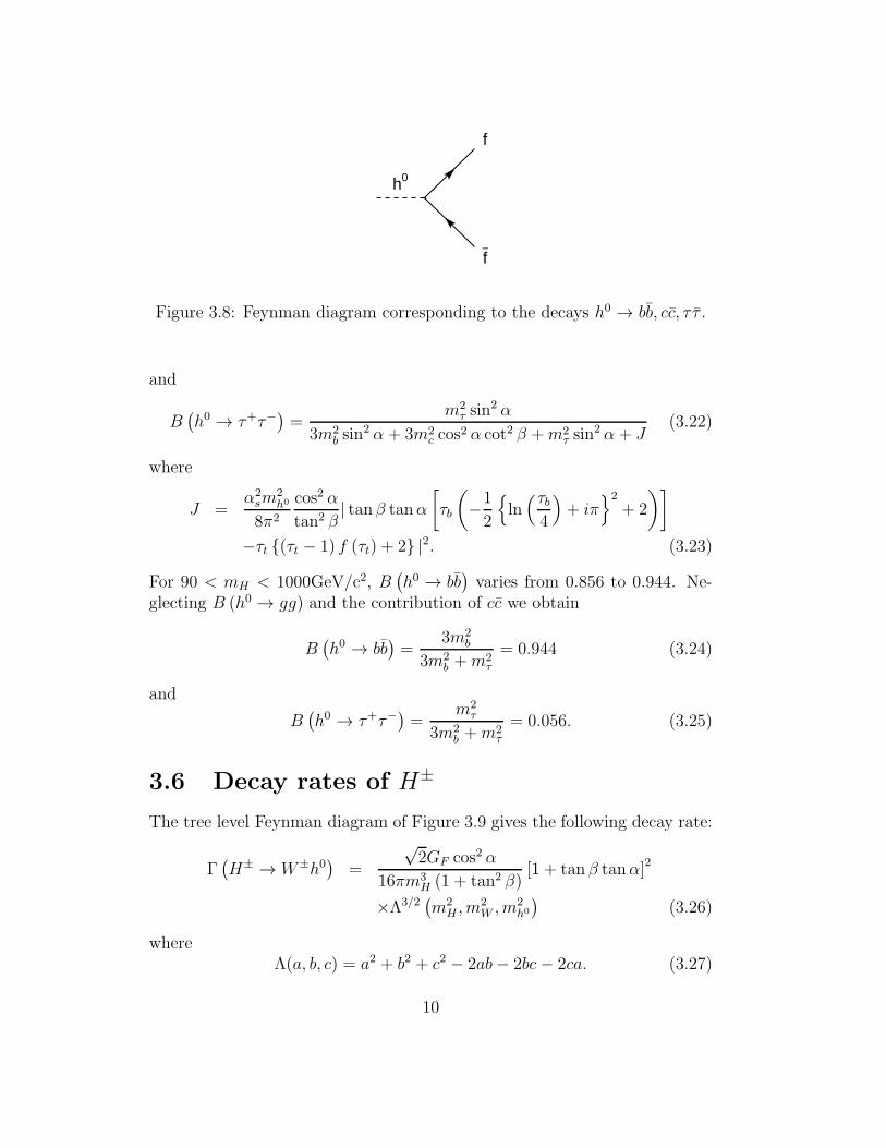
Figure 3.8: Feynman diagram corresponding to the decays h0 → bb, cc, τ τ .

and

B(

h0 → τ+τ−)

=m2

τ sin2 α

3m2b sin

2 α + 3m2c cos

2 α cot2 β +m2τ sin

2 α + J(3.22)

where

J =α2sm

2h0

8π2

cos2 α

tan2 β| tanβ tanα

[

τb

(

−12

ln(τb4

)

+ iπ2

+ 2

)]

−τt (τt − 1) f (τt) + 2 |2. (3.23)

For 90 < mH < 1000GeV/c2, B(

h0 → bb)

varies from 0.856 to 0.944. Ne-glecting B (h0 → gg) and the contribution of cc we obtain

B(

h0 → bb)

=3m2

b

3m2b +m2

τ

= 0.944 (3.24)

and

B(

h0 → τ+τ−)

=m2

τ

3m2b +m2

τ

= 0.056. (3.25)

3.6 Decay rates of H±

The tree level Feynman diagram of Figure 3.9 gives the following decay rate:

Γ(

H± →W±h0)

=

√2GF cos2 α

16πm3H (1 + tan2 β)

[1 + tan β tanα]2

×Λ3/2(

m2H , m

2W , m

2h0

)

(3.26)

whereΛ(a, b, c) = a2 + b2 + c2 − 2ab− 2bc− 2ca. (3.27)

10

H+/-

W+/-

h0

Figure 3.9: Feynman diagram corresponding to the decay H± →W±h0.

H+/-

W+/-

H0

Figure 3.10: Feynman diagram corresponding to the decay H± →W±H0.

Similarly from the Feynman diagrams of Figures 3.10 and 3.11 we obtain

Γ(

H± → W±H0)

=

√2GF (tanβ − tanα)2

16πm3H (1 + tan2 β) (1 + tan2 α)

×Λ3/2(

m2H , m

2W , m

2H0

)

, (3.28)

Γ(

H± → W±A0)

=

√2GF

16πm3H

Λ3/2(

m2A0 , m2

W , m2H

)

. (3.29)

3.7 Decays of H0.

The tree level Feynman diagrams of Figure 3.12 give the following decayrates:

Γ(H0 → f f) =

√2GFm

2fmH0

8π

(

1−4m2

f

m2H0

)3/2

NfB2f (3.30)

11

H+/-

W+/-

A0

Figure 3.11: Feynman diagram corresponding to the decay H± → W±A0.

where Nf = 3 for quarks, Nf = 1 for leptons, B2f = sin2 α(1 + cot2 β) for

f = u, c, t, and B2f = cos2 α(1 + tan2 β) for f = d, s, b, e−, µ−, τ−.

From the Feynman diagrams of Figure 3.13 we obtain

Γ(H0 → gg) =

√2GFα

2sm

3H0

64π3sin2 α(1 + cot2 β)

×| tan βtanα

τb [(τb − 1)f(τb) + 2]

+τt [(τt − 1)f(τt) + 2]|2 (3.31)

where

τi =4m2

i

m2H0

. (3.32)

From the Feynman diagram of Figure 3.14 we obtain

Γ(

H0 → h0h0)

=

√2GFm

4Z

32πmH0

×(

1− 4m2h0

m2H0

)1/2(1− tan2 α)

2

(1 + tan2 α)3(1 + tan2 β)

×[

4 tanα

1− tan2 α(tanα + tanβ)− (1− tanα tanβ)

]2

. (3.33)

From the Feynman diagrams of Figures 3.15 and 3.16 we obtain

Γ(

H0 → A0A0)

=

√2GFm

4Z

32πmH0

(

1− 4m2A0

m2H0

)1/2

× (tan2 β − 1)2

(1 + tan2 α) (1 + tan2 β)3 [1− tanα tanβ]2 , (3.34)

12

Γ(

H0 → ZZ)

=

√2GF (1 + tanβ tanα)2m3

H0

32π (1 + tan2 β) (1 + tan2 α)

×(

12x2 − 4x+ 1)

(1− 4x)1/2 (3.35)

where

x =m2

Z

m2H0

. (3.36)

Similarly, from the diagram of Figure 3.17 we obtain

Γ(

H0 → W+W−) =

√2GF (1 + tan β tanα)2m3

H0

16π (1 + tan2 β) (1 + tan2 α)

×(

12y2 − 4y + 1)

(1− 4y)1/2 (3.37)

where

y =m2

W

m2H0

. (3.38)

From the Feynman diagram of Figure 3.18 we obtain

Γ(

H0 → W±H∓) =

√2GF (tanα− tan β)2

16πm3H0 (1 + tan2 α) (1 + tan2 β)

×Λ3/2(

m2H0 , m2

W , m2H

)

. (3.39)

From the Feynman diagram of Figure 3.19 we obtain

Γ(

H0 → H+H−) =

√2GFm

4W

4πmH0 (1 + tan2 β) (1 + tan2 α)

×[

(1 + tanβ tanα)− (1− tanβ tanα)

2 cos2 θW

1− tan2 β

1 + tan2 β

]2

×(

1− 4m2H

m2H0

)1/2

. (3.40)

The Feynman diagrams corresponding to h0, H0 → γγ are shown in Fig-ure 3.20.

Γ(H0 → h0Z) = 0. (3.41)

3.8 Decay rates of A0

From the tree level Feynman diagram of Figure 3.21 we obtain

Γ(

A0 → Zh0)

=

√2GF cos2 α

16πm3A0 (1 + tan2 β)

× [1 + tan β tanα]2 Λ3/2(

m2A0 , m2

h0, m2Z

)

(3.42)

13

H0

f

f−

Figure 3.12: Feynman diagram corresponding to the decay H0 → f f .

H0i= b,t

g

i

gi

+H0

i = b,t

g

i

g

i

Figure 3.13: Feynman diagrams corresponding to the decay H0 → gg.

H0

h0

h0

Figure 3.14: Feynman diagram corresponding to the decay H0 → h0h0.

14

H0

A0

A0

Figure 3.15: Feynman diagram corresponding to the decay H0 → A0A0.

H0

Z0

Z0

Figure 3.16: Feynman diagram corresponding to the decay H0 → ZZ.

H0

W+

W-

Figure 3.17: Feynman diagram corresponding to the decay H0 →W+W−.

15

H0

W+/-

H-/+

Figure 3.18: Feynman diagram corresponding to the decay H0 →W±H∓.

H0

H+

H-

Figure 3.19: Feynman diagram corresponding to the decay H0 → H+H−.

16

H0,h0i = τ−,b,t

γ

i

γi

+H0,h0

i = τ−,b,t

γ

i

γ

i

H0,h0

W+/- γ

W+/-

γW+/-

+H0,h0

W+/-

γ

W+/-

γ

W+/-

H0,h0H+/- γ

H+/-

γH+/-

+H0,h0

H+/-

γ

H+/-

γ

H+/-

H0,h0

W+/- γ

γW+/-

+ H0,h0

H+/- γ

γH+/-

Figure 3.20: Feynman diagrams corresponding to h0, H0 → γγ.

17

From the tree level diagram of Figure 3.22 we obtain

Γ(

A0 → f f)

=

√2GF

8πmA0m2

fA2f

(

1−4m2

f

m2A0

)1/2

Nf (3.43)

where Nf = 3 for quarks, Nf = 1 for leptons, Af = cotβ for f = u, c, t,and Af = tanβ for f = d, s, b, e−, µ−, τ−.

From the Feynman diagrams shown in Figure 3.23 we obtain (see Ap-pendix D):

Γ(

A0 → Zγ)

=

√2GFα

2emm

3A0

512π3 sin2 θW cos2 θW

(

1− m2Z

m2A0

)3

×| tan β(

1

2− 2

3sin2 θW

)

I (τb,Λb)

+

(

1

2− 2 sin2 θW

)

I (ττ ,Λτ)

+2 cotβ

(

1

2− 4

3sin2 θW

)

I (τt,Λt) |2 (3.44)

where

τi =4m2

i

m2A0

, Λi =4m2

i

m2Z

, (3.45)

and

I (τi,Λi) =τiΛi

Λi − τif(τi)− f(Λi) . (3.46)

From the Feynman diagrams of Figure 3.24 we obtain the decay rate:

Γ(A0 → gg) =

√2GFα

2sm

3A0

128π3| tanβτbf(τb) + cot βτtf(τt)|2. (3.47)

Γ(

A0 → h0h0)

= Γ(

A0 → H0H0)

= 0. (3.48)

From the Feynman diagram 3.25 we obtain

Γ(

A0 →W±H∓) =

√2GF

16πm3A0

Λ3/2(

m2A0 , m2

W , m2H

)

. (3.49)

From the Feynman diagram 3.26 we obtain

Γ(

A0 → ZH0)

=

√2GF (tanβ − tanα)2

16πm3A0 (1 + tan2 α) (1 + tan2 β)

×Λ3/2(

m2A0 , m2

H0 , m2Z

)

. (3.50)

18

A0

Z0

h0

Figure 3.21: Feynman diagram corresponding to the decay A0 → Zh0.

A0

f

f−

Figure 3.22: Feynman diagram corresponding to the decay A0 → f f .

From the Feynman diagrams of 3.27 we obtain:

Γ(

A0 → γγ)

=

√2GFα

2emm

3A0

256π3

∣

∣

∣

∣

tanβ

[

1

3τbf(τb) + ττf(ττ )

]

+cotβ

[

4

3τtf(τt)

]∣

∣

∣

∣

2

(3.51)

19

A0 i = τ−,b,t

Z0

i

γi

+A0 i = τ−,b,t

γ

i

Z0

i

Figure 3.23: Feynman diagrams corresponding to the decay A0 → Zγ.

A0i= b,t

g

i

gi

+A0

i = b,t

g

i

g

i

Figure 3.24: Feynman diagrams of A0 → gg.

A0

W+/-

H-/+

Figure 3.25: Feynman diagram of A0 →W±H∓.

20

A0

Z0

H0

Figure 3.26: Feynman diagram of A0 → ZH0.

A0i= τ−,b,t

γ

i

γi

+A0

i = τ−,b,t

γ

i

γ

i

Figure 3.27: Feynman diagrams for A0 → γγ.

21

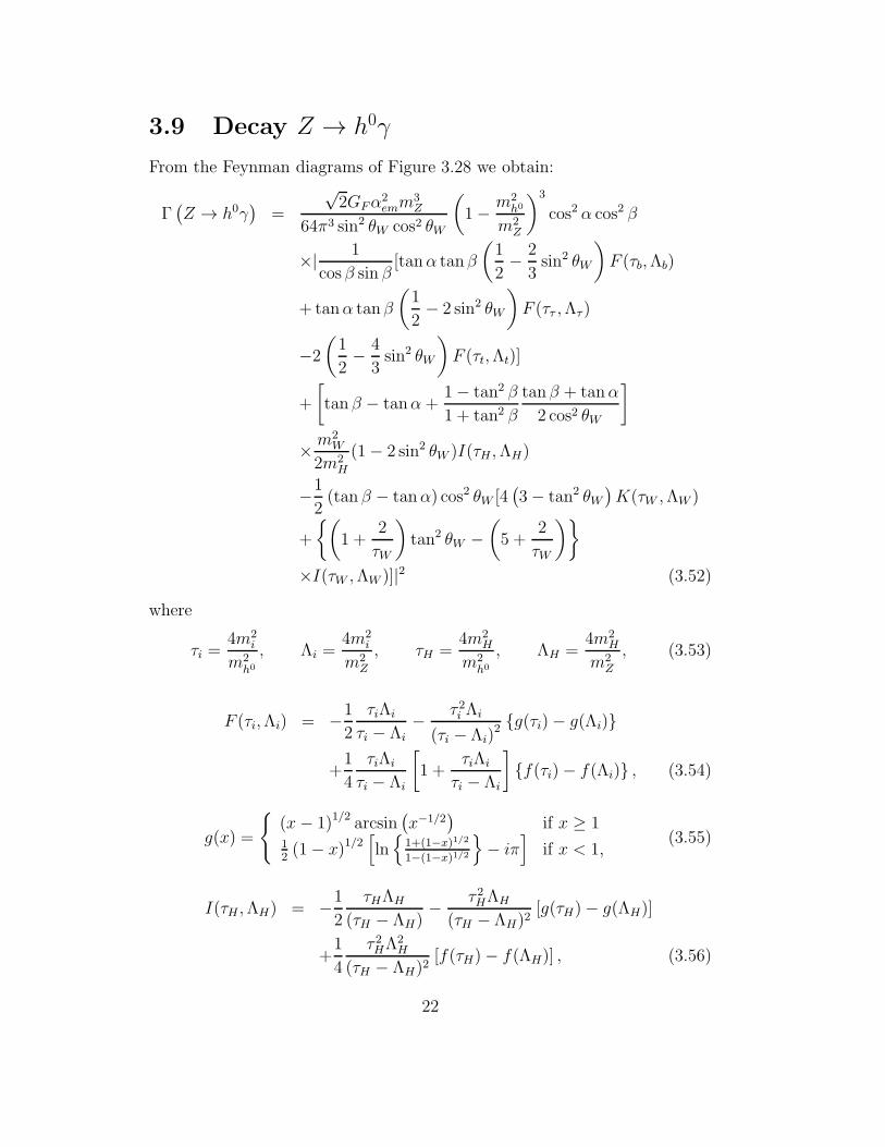
3.9 Decay Z → h0γ

From the Feynman diagrams of Figure 3.28 we obtain:

Γ(

Z → h0γ)

=

√2GFα

2emm

3Z

64π3 sin2 θW cos2 θW

(

1− m2h0

m2Z

)3

cos2 α cos2 β

×| 1

cos β sin β[tanα tanβ

(

1

2− 2

3sin2 θW

)

F (τb,Λb)

+ tanα tanβ

(

1

2− 2 sin2 θW

)

F (ττ ,Λτ)

−2(

1

2− 4

3sin2 θW

)

F (τt,Λt)]

+

[

tanβ − tanα +1− tan2 β

1 + tan2 β

tanβ + tanα

2 cos2 θW

]

× m2W

2m2H

(1− 2 sin2 θW )I(τH ,ΛH)

−12(tan β − tanα) cos2 θW [4

(

3− tan2 θW)

K(τW ,ΛW )

+

(

1 +2

τW

)

tan2 θW −(

5 +2

τW

)

×I(τW ,ΛW )]|2 (3.52)

where

τi =4m2

i

m2h0

, Λi =4m2

i

m2Z

, τH =4m2

H

m2h0

, ΛH =4m2

H

m2Z

, (3.53)

F (τi,Λi) = −12

τiΛi

τi − Λi− τ 2i Λi

(τi − Λi)2 g(τi)− g(Λi)

+1

4

τiΛi

τi − Λi

[

1 +τiΛi

τi − Λi

]

f(τi)− f(Λi) , (3.54)

g(x) =

(x− 1)1/2 arcsin(

x−1/2)

if x ≥ 112(1− x)1/2

[

ln

1+(1−x)1/2

1−(1−x)1/2

− iπ]

if x < 1,(3.55)

I(τH ,ΛH) = −12

τHΛH

(τH − ΛH)− τ 2HΛH

(τH − ΛH)2[g(τH)− g(ΛH)]

+1

4

τ 2HΛ2H

(τH − ΛH)2[f(τH)− f(ΛH)] , (3.56)

22

τW =4m2

W

m2h0

, ΛW =4m2

W

m2Z

, (3.57)

K(τW ,ΛW ) = − τWΛW

4(τW − ΛW )[f(τW )− f(ΛW )]. (3.58)

The decay width of Equation 3.52 turns out to be negligible compared to thefull width of Z so we can not use it to constrain the mass of h0.

3.10 Vertex with four particles

The decay rate corresponding to the Feynman diagram 3.29 is:

Γ(

H± →W±γh0)

=3G2

F sin2 θW (1 + tan β tanα)2m5W

32 (1 + tan2 β) (1 + tan2 α)π3 (xWH )1/2

×12Λ

1

2

(

1, xWH , xh0

H

)(

1 + xWH + xh0

H

)

+(

2xWH xh0

H − xWH − xh0

H

)

× ln

∣

∣

∣

∣

∣

∣

Λ1

2

(

1, xWH , xh0

H

)

+ 1− xWH − xh0

H

2(

xWH xh0

H

)1/2

∣

∣

∣

∣

∣

∣

−∣

∣

∣xh

0

H − xWH∣

∣

∣×

ln

∣

∣

∣

∣

∣

∣

∣

∣

∣

∣xh

0

H − xWH∣

∣

∣Λ

1

2

(

1, xWH , xh0

H

)

−(

xWH + xh0

H

)

+(

xWH − xh0

H

)2

2(

xWH xh0

H

)1/2

∣

∣

∣

∣

∣

∣

∣

(3.59)

where

xWH =m2

W

m2H

, xh0

H =m2

h0

m2H

. (3.60)

3.11 Production of h0, H0 and A0

From the Feynman diagrams in Figure 3.30 we obtain

σ (pp→ AX) =π2Γ (A→ 2g)γA

8m3A

×∫ 1

γA

dxaxa

g(

xa, m2)

g

(

γAxa, m2

)

+4π2γA3m3

A

×[

∑

q=u,d,s,c,b

Γ (A→ qq)

∫ 1

γA

dxaxa

fq(

xa, m2)

fq

(

γAxa, m2

)

]

(3.61)

23

Z0 i = τ−,b,th0

i

γi

+Z0 i = τ−,b,t

γ

i

h0

i

Z0 W+/- h0

W+/-

γW+/-

+Z0

W+/-

γ

W+/-

h0

W+/-

Z0 H+/- h0

H+/-

γH+/-

+Z0 H+/-

γ

H+/-

h0

H+/-

Z0

γ

W+/-

h0

W+/-

+Z0

γ

H+/-

h0

H+/-

Figure 3.28: Feynman diagrams for Z → h0γ.

24

H+/-

γ

W+/-

h0

Figure 3.29: Diagram for H± →W±γh0.

where A ≡ h0, H0, A0 and γA ≡ m2A/s. Here fq is the unpolarized parton

distribution function for quark or anti-quark q and g is the parton distributionfunction for gluons. m2 is the factorization scale. Γ(h0 → gg) is given by(3.12), Γ(H0 → gg) by (3.31), Γ(A0 → gg) by (3.47), Γ (h0 → cc) by (3.18),Γ(

h0 → bb)

by (3.19), Γ(H0 → qq) by (3.30), and finally, Γ (A0 → qq) isgiven by (3.43).

3.12 Production of h0Z0X

A production channel with interesting experimental signature ispp → h0Z0X . The differential cross section obtained from the Feynmandiagrams in Figure 3.3 is

d2σ

dyd (pT )2 =

∑

f

∫ 1

xamin

dxaff(

xa, m2a

)

ff(

xb, m2b

) xbs

m2h0 − u

×dσdt

(

f f → h0Z0)

(3.62)

where f is q or g,

xamin =

√smT e

y +m2h0 −m2

Z

s−√smT e−y, (3.63)

mT =(

m2Z + p2T

) 1

2 , (3.64)

xb =xa√smT e

−y +m2h0 −m2

Z

xas−√smT ey

, (3.65)

25

p g

i= b,tH0, h0, A0

gp−

+

p

qH0, h0, A0

q−

p−

Figure 3.30: Feynman diagrams for pp→ AX with A ≡ h0, H0, A0.

26

f t3L (f) qf gfA gfVe−, µ−, τ− −1

2−1 −1

2−1

2+ 2 sin2 θW

u, c, t 12

23

12

12− 4

3sin2 θW

d, s, b −12

−13−1

2−1

2+ 2

3sin2 θW

Table 3.1: Coefficients in Equation (3.70).

s = xaxbs, (3.66)

p2T =Λ(

s, m2h0 , m2

Z

)

sin2 θ

4s, (3.67)

u =1

2

(

m2h0 +m2

Z − s− cos θΛ1/2(s, m2h0, m2

Z))

(3.68)

andut = m2

h0m2Z + sp2T . (3.69)

y is the rapidity, θ is the angle of dispersion, and pT is the transverse mo-mentum of Z0. For the light quarks u, d and s we obtain

dσ

dt=

1

48πsG2

Fm4Z

sin2 (β − α)(s−m2

Z)2+m2

ZΓ2Z

[

(

gfV

)2

+(

gfA

)2]

×[

8m2Z +

Λ(

s, m2h0 , m2

Z

)

ssin2 θ

]

(3.70)

where gfA ≡ t3L (f) and gfV ≡ t3L (f) − 2qf sin

2 θW . Coefficients in Equation(3.70) are given in Table 3.1. The Standard Model cross section is obtainedby omitting the factor sin2 (β − α) in Equation (3.70). The contributions tothe cross section from the heavy quarks c and b are negligible. ΓZ is the totaldecay width of the Z0.

3.13 Production of H+

From the diagrams in Figures 3.31 and 3.32 we obtain

σ(pp→ H+X) =4π2γH3m3

H

∑

q,q′

Γ(H+ → qq′)

∫ 1

γH

dxaxa

[

f pq (xa, m

2) · f pq′(γHxa, m2) + f p

q′(xa, m2) · f p

q (γHxa, m2)

]

(3.71)

27

p

qH+

q’−

p−

Figure 3.31: Feynman diagram for pp→ H+X .

H+

f

f’−

Figure 3.32: Feynman diagram for H+ → f f ′.

28

where

γH =m2

H

s(3.72)

and

Γ(H+ → f f ′) = Γ(H− → f ′f)

=

√2GF |Vff ′ |2Nc

16πmH· Λ1/2

(

m2f

m2H

,m2

f ′

m2H

, 1

)

×

A2[

m2H − (mf +mf ′)2

]

+B2[

m2H − (mf −mf ′)2

]

(3.73)

with Nc = 3 for quarks, Nc = 1 for leptons,

A = mf ′ tanβ +mf cot β (3.74)

B = mf ′ tan β −mf cot β (3.75)

f = u, c, t, νe, νµ, ντ , and f′ = d, s, b, e−, µ−, τ−.[7]

3.14 Production of h0W+X

Let us now consider the channel pp→ h0W+X . We obtain:

d2σ

dyd (pT )2 =

∑

q,q′

∫ 1

xamin

dxa[fpq

(

xa, m2a

)

f p

q′

(

xb, m2b

)

+f p

q′

(

xa, m2a

)

f pq

(

xb, m2b

)

]xbs

m2h0 − u

dσ

dt

(

qq′ → h0W+)

(3.76)

wheref pq′ = f p

q′, f p

q = f pq , f p

q = f pq , f p

q′ = f p

q′, (3.77)

xamin =

√smT e

y +m2h0 −m2

W

s−√smT e−y, (3.78)

mT =(

m2W + p2T

)1

2 , (3.79)

xb =xa√smT e

−y +m2h0 −m2

W

xas−√smT ey

, (3.80)

s = xaxbs, (3.81)

29

p2T =Λ(

s, m2h0 , m2

W

)

sin2 θ

4s, (3.82)

u =1

2

[

m2h0 +m2

W − s− cos θΛ1/2(s, m2h0 , m2

W )]

, (3.83)

t =1

2

[

m2h0 +m2

W − s+ cos θΛ1/2(s, m2h0 , m2

W )]

, (3.84)

cos θ =

(

1− 4sp2TΛ(s, m2

h0, m2W )

)1/2

(3.85)

andut = m2

h0m2W + sp2T . (3.86)

y is the rapidity of W+ and pT is the transverse momentum of W+. Fromthe Feynman diagrams of Figure 3.6 we obtain for f f ′ → h0W+:

dσ

dt=

1

16πs2|Vff ′ |2G2

F|CH+ |2 sΛ

×[

m2f ′ tan2 β +m2

f cot2 β]

+m4W |CW |2

[

8sm2W + Λ sin2 θ

]

−2CH+ℜ(CW )[m2f ′ tan β(sΛ + 2m2

W u(

s−m2h0

)

+2m4W

(

2m2h0 − t

)

)−m2f cot β(sΛ+ 2m2

W t(

s−m2h0

)

+2m4W

(

2m2H0 − u

)

)]

+1

2m2

WΛ sin2 θ

[

m2fC

2f

t2+m2

f ′C2f ′

u

]

+ s[

m2fC

2f +m2

f ′C2f ′

]

+2CH+ s

[

m2h0m2

W −1

4Λ sin2 θ

] [

m2f cot βCf

t−m2

f ′ tan βCf ′

u

]

+2CH+ s[

m2f ′ tanβCf ′u−m2

f cot βCf t]

−2ℜ(CW )

[

1

2Λ sin2 θ

(

m2W +

s

2

)

− sm2h0m2

W + 4sm4W + 4m6

W

]

×[

m2fCf

t+m2

f ′Cf ′

u

]

− 2ℜ(CW )m2fCf

[

−2m4W + t

(

s− 2m2W

)]

−2ℜ(CW )m2f ′Cf ′

[

−2m4W + u

(

s− 2m2W

)]

(3.87)

where Λ stands for Λ(s, m2h0, m2

W ),

CH+ =cos (β − α)s−m2

H

, (3.88)

30

partons tan(β) = 100 tan(β) = 10 tan(β) = 2gg 0.20E+1 0.13E-1 0.35E-1bb 0.31E+2 0.31E+0 0.12E-1cc 0.73E-7 0.73E-5 0.18E-3ss 0.20E+0 0.20E-2 0.81E-4dd 0.10E-1 0.10E-3 0.41E-5uu 0.18E-9 0.18E-7 0.46E-6

Table 3.2: Production cross section [pb] for pp → A0 from the indicatedpartons. mA0 = 200GeV/c2,

√s = 1960GeV/c2.

CW =sin (β − α) (s−m2

W − imWΓW )

(s−m2W )

2+m2

WΓ2W

, (3.89)

Cf = −cosαsin β

, Cf ′ =sinα

cos β. (3.90)

For pp→ h0W−X interchange u↔ t.For the Standard Model we obtain the differential cross section (3.87)

with h0 replaced by the Standard Model Higgs, CH+ = 0, Cf = Cf ′ = −1,and sin(β − α) = 1 in (3.89).

3.15 Numerical examples

Two sensitive channels for the search of the Standard Model Higgs are pp→h0ZX and pp→ h0W±X . The cross section for pp→ h0ZX off resonance inthe Doublet model differs from the Standard Model by a factor sin2(β − α)(see Equation (3.70)) and it will be hard to obtain both mh0 and tan(β). Weare therefore interested in the production of h0Z on resonance. In particularpp → A0 followed by A0 → h0Z → bbl−l+ where l = µ, e. A peak shouldbe observed in the h0Z invariant mass. From Equation (3.61) we obtain thecross sections listed in Tables 3.2 and 3.3.

Let us now consider the decays of A0. As an example we take mh0 =120GeV/c2, mH0 = 250GeV/c2, mH = 200GeV/c2 and mA0 = 250GeV/c2.The corresponding branching fractions are listed in Table 3.4. From Tables3.3 and 3.4 we obtain a production cross section times branching fraction forthe process pp → A0 → h0Z of 0.018pb for tan(β) = 2, and 0.0045pb fortan(β) = 10.

From Equations (3.71) and (3.73) we obtain the production cross sectionsfor pp→ H+X shown in Table 3.5.

31

partons tan(β) = 100 tan(β) = 10 tan(β) = 2gg 0.42E+0 0.22E-2 0.19E-1bb 0.82E+1 0.82E-1 0.33E-2cc 0.19E-7 0.19E-5 0.49E-4ss 0.57E-1 0.57E-3 0.23E-4dd 0.44E-2 0.44E-4 0.18E-5uu 0.89E-10 0.89E-8 0.22E-6

Table 3.3: Production cross section [pb] for pp → A0 from the indicatedpartons. mA0 = 250GeV/c2,

√s = 1960GeV/c2.

partons tan(β) = 100 tan(β) = 10 tan(β) = 2A→ gg 3.0E-4 1.5E-4 2.0E-3A→ bb 1.0E+0 9.4E-1 5.9E-2A→ cc 8.0E-10 7.5E-6 2.9E-4A→ ss 8.0E-4 7.5E-4 4.7E-5A→ Zh0 6.1E-6 5.5E-2 9.4E-1A→ Zγ 1.9E-8 6.0E-9 1.2E-6A→ γγ 1.2E-7 8.1E-8 7.5E-6

Table 3.4: Branching fractions for A0 assuming mH = 200GeV/c2, mH0 =250GeV/c2, mA0 = 250GeV/c2 and mh0 = 120GeV/c2.

partons tan(β) = 100 tan(β) = 10 tan(β) = 2ud 0.82E-2 0.82E-4 0.34E-5us 0.66E-1 0.66E-3 0.26E-4ub 0.89E-2 0.89E-4 0.36E-5cs 0.31E-1 0.32E-3 0.91E-4cb 0.24E-1 0.24E-3 0.96E-5

Table 3.5: Production cross section [pb] for pp → H+X from the indicatedpartons. mH = 250GeV/c2,

√s = 1960GeV/c2.

32

process tan(β) = 100 tan(β) = 50 tan(β) = 2b+ g → b+ h0 0.021 0.021 0.011

u+ u→ b+ b+ h0 0.002 0.001 0.0004d+ d→ b+ b+ h0 0.0005 0.0005 0.0001g + g → b+ b+ h0 0.015 0.015 0.008

Table 3.6: Production cross section [pb] for pp → bh0X from the indicatedprocesses. mh0 = 120GeV/c2, mA0 = 250GeV/c2,

√s = 1960GeV/c2.

Other channels of experimental interest are the production of 3 or moreb-jets as in Figure 3.33. Some numerical calculations using the CompHEPprogram[8] are presented in Table 3.6.

3.16 Running coupling constants and Grand

Unification

The coupling constants of the Two Higgs Doublet Model of type II are gs(µ)for SU(3), g(µ) for SU(2), and g′(µ) for U(1). These coupling constantsdepend on the energy scale µ as follows:

1

g2s(µ)=

1

g2s(mx)+

1

8π2

(

−11 + 4

3nF

)

ln

(

mx

µ

)

, (3.91)

1

g2(µ)=

1

g2(mx)+

1

8π2

(

−223

+4

3nF +

1

6nS

)

ln

(

mx

µ

)

, (3.92)

1

g′2(µ)=

1

g′2(mx)+

1

8π2

(

20

9nF +

1

6nS

)

ln

(

mx

µ

)

, (3.93)

where nF is the number of families of quarks and leptons, and nS is thenumber of higgs doublets. For the Two Higgs Doublet Model of type II con-sidered in this article, nF = 3 and nS = 2. In terms of the elementary elec-tric charge and the Weinberg angle, g(mZ) = e(mZ)/ sin θW (mZ), g

′(mZ) =e(mZ)/ cos θW (mZ). The fine structure constant is α(mZ) = e2(mZ)/(4π).

Let us now assume that a Grand Unified Theory (GUT) breaks its sym-metry to SU(3)×SU(2)×U(1) at the energy scale mx. At this scale we take

g2s(mx) = g2(mx) =5

3g′2(mx), (3.94)

33

g b

b

h0

b

b−

g

q

q−

g b h0b

b−

b h0

b

g

b

b

g

bh0

b

Figure 3.33: Some Feynman diagrams for the production of three or moreb-jets.

34

Doublet Model MSSMnS sin2 θW (mZ) mx sin2 θW (mZ) mx

0 0.2037 1.0 · 1015 0.2037 8.0 · 10172 0.2118 4.2 · 1014 0.2311 2.0 · 10164 0.2194 1.8 · 1014 0.2536 1.0 · 10156 0.2266 8.3 · 1013 0.2722 8.3 · 10138 0.2334 3.9 · 1013 0.2880 1.0 · 1013

Table 3.7: Predicted sin2 θW (mZ) and mx for the Two Higgs Doublet Modelof type II, and the Minimum Supersymmetric Model as a function of thenumber of doublets nS.

and obtain

sin2 θW =11 + 1

2nS + 5e2

3g2s

(

22− 15nS

)

66 + nS

, (3.95)

ln

(

mx

mZ

)

=24π2

e2

1− 8e2

3g2s

66 + nS, (3.96)

with all running couplings evaluated at mZ .The corresponding equations of the Minimum Supersymmetry Model[9]

are

sin2 θW =18 + 3nS + e2

g2s(60− 2nS)

108 + 6nS

, (3.97)

ln

(

mx

mZ

)

=8π2

e2

[

1− 8e2

3g2s

18 + nS

]

. (3.98)

Some numerical results are presented in Table 3.7. From the Table weconclude that the Two Higgs Doublet Model of type II is in disagreementwith the measured value of sin2 θW (mZ), and with the non-observation ofproton decay (mx is too low). Raising the number of doublets to ≈ 7 wouldbring sin2 θW (mZ) into agreement with observations, but mx is still too low.The MSSM with nS = 2 (which includes the Two Higgs Doublet Model oftype II) is in agreement with both the observed sin2 θW (mZ), and with thenon-observation of proton decay.

3.17 Conclusions

One of the major efforts at the Fermilab Tevatron in Run II, and at thefuture LHC, is the search for the Standard Model Higgs hSM . The four

35

channels with largest production cross section are[6] gg → hSM , qq′ →hSMW , qq → hSMZ and qq → hSMqq. The decay modes of hSM withlargest branching fraction[6] are bb for mhSM

. 137GeV/c2 and W+W− formhSM

& 137GeV/c2.The search for the Standard Model Higgs will also constrain or discover

particles of the Two Higgs Doublet Model of type II.The most interesting production channels are gg → h0, H0, A0 on mass

shell, and qq, gg → h0Z and qq′ → h0W± in the continuum (tho there maybe peaks at mA0). The most interesting decays are h0, H0, A0 → bb-jets andτ+τ−, and, if above threshold, H0 → ZZ, W+W− and h0h0. The followingfinal states should be compared with the Standard Model cross section: bbZ,bbW±, τ+τ−Z, τ+τ−W±, bb, τ+τ−, ZZ, W+W−, 3 and 4 b-jets, 2τ+ + 2τ−,bbτ+τ−, ZW+W−, 3Z, ZZW± and 3W±. Mass peaks should be searched inthe following channels: Zbb, ZZ, ZZZ, bb, 4b-jets and, just in case, Zγ.

We have discussed the masses of the Higgs particles in the Two HiggsDoublet Model of type II, and have calculated several relevant productioncross sections and decay rates. We have also discussed running couplingconstants and Grand Unification. If the Two Higgs Doublet Model of type IIis part of a Grand Unified Theory, then it does not agree with the observedsin2 θW nor with the non-observation of proton decay. The MSSM with nS =2 (which includes the Two Higgs Doublet Model of type II) is in agreementwith both the observed sin2 θW (mZ), and with the non-observation of protondecay.

36

Bibliography

[1] Vernon Barger and Roger Phillips, Collider Physics (Addison Wesley,1988), pages 452-454; S. Dawson, J. F. Gunion, H.E. Haber and G.Kane, The Higgs Hunter’s Guide (Addison Wesley, 1990), p. 201.

[2] Carlos A. Marın and Bruce Hoeneisen, hep-ph/0210167 (2002).

[3] CDF Collab., Phys. Rev. Lett. 79, 357 (1997).

[4] D0 Collab., Phys. Rev. Lett. 82, 4975 (1999); FERMILAB-Conf-00-294-E.

[5] LEP Higgs Working Group, http://lephiggs.web.cern.ch/LEPHIGGS/papers/index.html; LHWG Note/2001-05.

[6] Review of Particle Physics, K. Hagiwara et al, Physical Review D66,010001 (2002).

[7] Carlos Marın y Guillermo Hernandez, Serie de Documentos USFQ 13,Universidad San Francisco de Quito, Ecuador (1994)

[8] “CompHEP: A package for evaluation of Feynman diagrams and integra-tion over multiparticle phase space.” A. Pukhov, E. Boos, M. Dubinin,V. Edneral, V. Ilyin, D. Kovalenko, A. Kryukov, V. Savrin, S. Shichanin,A. Semenov, hep-ph/9908288 (1999)

[9] “The quantum theory of fields”, Volume III, Supersymmetry, StevenWeinberg, Cambridge University Press (2000).

37

Chapter 4

Higgs production at a muon

collider in the Two Higgs

Doublet Model of type II

Abstract

We calculate Higgs production cross sections at a muon collider in the TwoHiggs Doublet Model of type II. The most interesting productions channelsare µ−µ+ → h0Z0, H0Z0, H−H+, A0Z0 and H∓W±. The last channel iscompared with the production processes pp→ H∓W±X and pp→ H∓W±Xat the Tevatron and LHC energies, respectively, for large values of tan β.

4.1 Introduction

In this article we calculate neutral and charged Higgs production cross sec-tions at a muon collider in the Two Higgs Doublet Model of type II. TheHiggs sector of the Minimal Supersymmetric Standard Model (MSSM) is ofthis type (tho the model of type II does not require Supersymmetry). Higgsdoublets can be added to the Standard Model without upsetting the Z/Wmass ratio. Higher dimensional representations upset this ratio [1]. Adding asecond complex doublet to the Standard Model results in five Higgs bosons:one pseudoscalar A0 (CP-odd scalar), two neutral scalars H0 and h0 (CP-even scalars), and two charged scalars H+ and H−. In the Standard Modelwe only have a single neutral Higgs.

In recent years, some papers have appeared, suggesting the possibilityof the construction of a µ−µ+ collider to detect charged or neutral Higgsbosons [[2], [3]]. The main reason is that in a muon collider, the signal couldbe cleaner than in a hadron collider. In this paper, we analyze this possibilitystudying some production cross sections like: µ−µ+ → h0Z0, H0Z0, H−H+,A0Z0 and H∓W± (Sections 4.2-4.6).

In Sections 4.5,4.6,4.8,4.9 we will focus our interest in the production ofcharged Higgs bosons. There are three ways of producing H±. One is viapp or pp interactions in a hadron collider. In hadron colliders, the signalsare overwhelmed by backgrounds due basically to tt production [4]. Theother ways to produce charged Higgs are e−e+ or µ−µ+ colliders , in whichbackgrounds are considerably less. In some processes like µ−µ+ → H−H+

and e−e+ → H−H+, there is no difference between the cross sections obtainedin an e−e+ collider or a µ−µ+ collider. However, in reactions like µ−µ+ →H∓W± and e−e+ → H∓W±, the total cross section is proportional to thesquare of the mass of the fermion and then e−e+ interactions give us verysmall cross sections. This motivated us to compare in Section 4.9 the channelµ−µ+ → H∓W± (at

√s = 500GeV/c and for large values of tanβ) with the

production processes pp → H∓W±X (at the Tevatron) and pp→ H∓W±X(at the LHC), to check the feasibility of detecting H± using a muon collider.

The influence of radiative corrections in the masses of the Higgs bosonsis considered in all the calculations.

1

4.2 Higgs bosons masses and radiative cor-

rections

The masses of the neutral Higgs particles, calculated at tree level, are [5]:

m2A0 = m2

H −m2W (4.1)

m2H0 =

1

2

[

m2Z +m2

A0 +[

(

m2Z −m2

A0

)2+ 4m2

A0m2Z sin2 2β

]1/2]

(4.2)

m2h0 =

1

2

[

m2Z +m2

A0 −[

(

m2Z −m2

A0

)2+ 4m2

A0m2Z sin2 2β

]1/2]

(4.3)

with 0 ≤ β < π2

From these relations, the Higgs bosons masses satisfy the bounds:

mA0 < mH (4.4)

mH > mW (4.5)

mh0 ≤ mZ (4.6)

mZ ≤ mH0 ≤ sec θWmH (4.7)

The bound given by (4.6) practically has been excluded by the presentlimits on mh0 obtained by LEP and CDF [6].

The mixing angle α (−π/2 < α ≤ 0) between the two neutral scalar Higgsfields H0, h0 is given by

tanα = −[

1 + F

1− F

]1/2

(4.8)

F =(1− tan2 β)

(1 + tan2 β)G

[

1− m2Z

m2H

− m2W

m2H

]

(4.9)

G =

[

(

1− m2W

m2H

+m2

Z

m2H

)2

− 4

(

m2Z

m2H

)(

1− m2W

m2H

)(

1− tan2 β

1 + tan2 β

)2]1/2

(4.10)

2

In terms of mH and G Equations (4.2) and (4.3) are:

m2H0 =

1

2m2

H

[

1− m2W

m2H

+m2

Z

m2H

+ G

]

(4.11)

m2h0 =

1

2m2

H

[

1− m2W

m2H

+m2

Z

m2H

−G]

(4.12)

Taking into account radiative corrections, (4.2) and (4.3) can be writtenas [see [7], [8]]:

m2H0 =

1

2m2

A +m2Z +∆t +∆b

+((

m2A −m2

Z

)

cos 2β +∆t −∆b

)2

+(

m2A +m2

Z

)2sin2 2β1/2 (4.13)

m2h0 =

1

2m2

A +m2Z +∆t +∆b

−((

m2A −m2

Z

)

cos 2β +∆t −∆b

)2

+(

m2A +m2

Z

)2sin2 2β1/2 (4.14)

where:

∆b =3√2m4

bGF (1 + tan2 β)

2π2ln

(

M2sb

m2b

)

(4.15)

and

∆t =3√2m4

tGF (1 + tan2 β)

2π2 tan2 βln

(

M2st

m2t

)

(4.16)

Msb andMst are the masses of the sbottom and stop (the scalar superpartnersof the bottom and top quarks).

Equation (4.1) is practically unaffected by radiative corrections. Accord-ing to (4.14) mh0 increases as the value of mA increases. Then, for very largevalues of mA we can set an upper bound for mh0 :

m2h0 ≤ m2

h0(mA0 →∞) = m2Z

(

1− tan2 β

1 + tan2 β

)2

+∆t tan

2 β

(1 + tan2 β)+

∆b

(1 + tan2 β)(4.17)

3

Taking mb = 4.3 GeV/c2, mt = 174.3GeV/c2, Mst ∼ Msb ∼ 1TeV [7] andmZ = 91.1876GeV/c2 we obtain:

∆b = 1.123× 10−6(

1 + tan2 β)

m2Z (4.18)

∆t = 0.9723m2Z

(1 + tan2 β)

tan2 β(4.19)

The contribution of the b-quark loop is negligible. Using Equations (4.18)and (4.19), (4.17) can be expressed as:

mh0 ≤ mZ

[

(

1− tan2 β

1 + tan2 β

)2

+ 0.9723

]1/2

(4.20)

For large values of tan β (tan β →∞) we obtain the limit

mh0 ≤ 1.4044mZ = 128.062GeV/c2 (4.21)

The upper bound on mh0 is raised by radiative corrections from mZ to128.062 GeV/c2 for stop masses of order 1 TeV.

Considering radiative corrections, we can write, for the masses of theneutral Higgs scalars:

m2H0 =

1

2m2

H

[

1− m2W

m2H

+m2

Z

m2H

+∆t

m2H

+Grc

]

(4.22)

m2h0 =

1

2m2

H

[

1− m2W

m2H

+m2

Z

m2H

+∆t

m2H

−Grc

]

(4.23)

Grc = [

(

1− m2W

m2H

+m2

Z

m2H

)2

− 4

(

m2Z

m2H

)(

1− m2W

m2H

)(

1− tan2 β

1 + tan2 β

)2

+2

(

∆t

m2H

)(

1− m2W

m2H

− m2Z

m2H

)(

1− tan2 β

1 + tan2 β

)

+

(

∆t

m2H

)2

]1/2 (4.24)

With radiative corrections, the value of the α parameter is:

tanα = −[

1 + Frc

1− Frc

]1/2

(4.25)

Frc =

[(

1−tan2 β1+tan2 β

)(

1− m2Z

m2H− m2

W

m2H

)

+ ∆t

m2H

]

Grc(4.26)

4

Additionally we have:

sin 2α = − 2 tanβ

(1 + tan2 β)

(

1− m2W

m2H+

m2Z

m2H

)

Grc(4.27)

4.3 Production of h0 , H0

From the Feynman diagrams in Figure 4.1 and the corresponding Feynmanrules given in reference [9], we obtain the differential cross section for thereaction µ−µ+ → h0Z0 in the center of mass system

dσ

dΩ(µ−µ+ → h0Z0) =

1

64π2s2G2

Fm4Z |CZ |2 Λ1/2(s,m2

h0, m2Z)

[

(gµA)2 + (gµV )

2]

[

8sm2Z + Λ(s,m2

h0, m2Z)sin

2θ]

(4.28)

where

gµA = −12

gµV = −12+ 2 sin2 θW (4.29)

Λ(a, b, c) = a2 + b2 + c2 − 2ab− 2ac− 2bc (4.30)

CZ =sin (β − α)

(s−m2Z + imZΓZ)

(4.31)

ΓZ is the total decay width of the Z0 and θ is the scattering angle in thecenter of mass system.

The total cross section corresponding to µ−µ+ → h0Z0 is obtained inte-grating Equation (4.28):

σ(µ−µ+ → h0Z0) =G2

Fm4Z (tan β − tanα)2

48πs2 (1 + tan2 α) (1 + tan2 β)

×(

1− 4 sin2 θW + 8 sin4 θW)

[

(s−m2Z)

2+m2

ZΓ2Z

]

[

12sm2Z + Λ(s,m2

h0, m2Z)]

×Λ1/2(s,m2h0, m2

Z)×(

3.8938× 1011)

fb (4.32)

In Figures 4.2 and 4.3 , the total cross section for µ−µ+ → h0Z0, isplotted as a functionmh0 for several values of

√s and tanβ. These total cross

5

µ−

µ+

A0h0,H0

Z0 +

µ−

µ+

Z0 h0,H0

Z0

µ− h0,H0

µ−

µ+Z0

+

µ−

Z0

µ−

h0,H0

µ+

Figure 4.1: Feynman diagrams corresponding to the production of h0 or H0

in the channel µ−µ+ → h0Z0.

sections were plotted considering the radiative corrections of the masses givenby Equations (4.23), (4.24), (4.25) and (4.26). According to these graphs,the total cross section becomes important in the mass interval 118 ≤ mh0 ≤128[GeV/c2].

The Standard Model cross section is:

σ(µ−µ+ → h0SMZ0)SM =

G2Fm

4Z

48πs2

(

1− 4 sin2 θW + 8 sin4 θW)

[

(s−m2Z)

2+m2

ZΓ2Z

]

×[

12sm2Z + Λ(s,m2

h0SM, m2

Z)]

×Λ1/2(s,m2h0SM, m2

Z)×(

3.8938× 1011)

fb (4.33)

where hSM is the Standard Model Higgs boson.The production cross section corresponding to e−e+ → h0Z0 is given by

an expression identical to (4.32). In terms of the cross section

6

0

10

20

30

40

50

60

85 90 95 100 105 110 115 120 125 130

σ[fb]

mh0 [GeV/c2]

σ(µ−µ+ → h0Z0)

√s = 500GeV/c, tanβ = 30

Figure 4.2: Total cross section for the process µ−µ+ → h0Z0 as a functionof mh0 . We have taken

√s = 500GeV/c and tanβ = 30.

0

10

20

30

40

50

60

70

80

90

100

85 90 95 100 105 110 115 120 125 130

σ[fb]

mh0 [GeV/c2]

σ(µ−µ+ → h0Z0)

√s = 400GeV/c, tanβ = 50

Figure 4.3: Total cross section for the process µ−µ+ → h0Z0 as a functionof mh0 . We have taken

√s = 400GeV/c and tanβ = 50.

7

0

0.02

0.04

0.06

0.08

0.1

0.12

0.14

0.16

85 90 95 100 105 110 115 120 125 130

σr

mh0 [GeV/c2]

σr =σ(e−e+→h0Z0)σ(e−e+→µ−µ+)

√s = 500GeV/c, tanβ = 30

Figure 4.4: Total cross section σ(e−e+ → h0Z0) compared with the cross sec-tion σ(e−e+ → µ−µ+) as a function of mh0 . We have taken

√s = 500GeV/c

and tan β = 30.

σ (e−e+ → µ−µ+) we can write:

σ (e−e+ → h0Z0)

σ (e−e+ → µ−µ+)=

1

128s

(tanβ − tanα)2

(1 + tan2 α) (1 + tan2 β)Λ1/2(s,m2

h0, m2Z)

×(

1− 4 sin2 θW + 8 sin4 θW)

sin4 θW(

1− sin2 θW)2

[

12sm2Z + Λ(s,m2

h0, m2Z)]

[

(s−m2Z)

2+m2

ZΓ2Z

] (4.34)

Equation (4.34) is plotted in Figure 4.4, as a function of mh0 for√s =

500GeV/c and tan β = 30.The total cross section corresponding to µ−µ+ → H0Z0 is obtained from

Equation (4.32) replacing (tanβ − tanα)2 by (1 + tanβ tanα)2 in the nu-merator and mh0 by mH0 . This production cross section is plotted in Figures4.5, 4.6 as a function ofmH0 for

√s = 500GeV/c and tan β = 30, without and

with mass radiative corrections, respectively. In Figure 4.7 we show the ratiobetween the production cross section σ (e−e+ → H0Z0) and the cross sectionσ (e−e+ → µ−µ+) in terms of mH0 . The radiatively corrected masses totalcross section is shown in Figure 4.8. Figures 4.6 and 4.8 show the importanceof the radiative corrections of the masses in the processes µ−µ+ → H0Z0 ande−e+ → H0Z0.

8

0

5

10

15

20

25

30

35

40

50 100 150 200 250 300

σ[fb]

mH0 [GeV/c2]

σ(µ−µ+ → H0Z0)

√s = 500GeV/c, tanβ = 30

Figure 4.5: Total cross section for the process µ−µ+ → H0Z0 as a functionof mH0 . The radiative corrections of the masses were not taken into account.We have taken

√s = 500GeV/c and tanβ = 30.

0

10

20

30

40

50

60

120 140 160 180 200 220 240 260

σ[fb]

mH0 [GeV/c2]

σ(µ−µ+ → H0Z0)

√s = 500GeV/c, tanβ = 30

Figure 4.6: Radiatively corrected masses total cross section for the processµ−µ+ → H0Z0 as a function of mH0 . We have taken

√s = 500GeV/c and

tan β = 30.

9

0

0.01

0.02

0.03

0.04

0.05

0.06

0.07

0.08

0.09

0.1

100 120 140 160 180 200 220 240 260 280

σro

mH0 [GeV/c2]

σro =σ(e−e+→H0Z0)σ(e−e+→µ−µ+)

√s = 500GeV/c, tanβ = 30

Figure 4.7: Total cross section for the process e−e+ → H0Z0 compared withthe cross section σ(e−e+ → µ−µ+) as a function of mH0 . We have taken√s = 500 GeV/c and tanβ = 30. The radiative corrections of the masses

were not taken into account.

10

0

0.02

0.04

0.06

0.08

0.1

0.12

0.14

0.16

100 120 140 160 180 200 220 240 260 280

σrc

mH0 [GeV/c2]

σrc =σ(e−e+→H0Z0)σ(e−e+→µ−µ+)

√s = 500GeV/c, tanβ = 30

Figure 4.8: Radiatively corrected masses total cross section for the processe−e+ → H0Z0 compared with the cross section σ(e−e+ → µ−µ+) as a func-tion of mH0 . We have taken

√s = 500GeV/c and tanβ = 30.

4.4 Production of A0

From the Feynman diagrams of Figure 4.9 and the Feynman rules givenin [9], we obtain the differential cross section for the production processµ−µ+ → A0Z0 in the center of mass system:

11

µ−

µ+

H0A0

Z0 +

µ−

µ+

h0A0

Z0

µ− A0

µ−

µ+Z0

+

µ−

Z0

µ−

A0

µ+

Figure 4.9: Feynman diagrams corresponding to the production of A0 in thechannel µ−µ+ → A0Z0.

dσ

dΩ(µ−µ+ → A0Z0) =

1

64π2sΛ1/2

(

s,m2A0, m2

Z

)

G2Fm

2µ

×C2HbΛ

(

s,m2A0, m2

Z

)

+[

(gµA)2+ (gµV )

2]

[tan2 β

(

1 +Λ(

s,m2A0 , m2

Z

)

m2Z sin2 θ

2st2

)

+ tan2 β

(

1 +Λ(

s,m2A0, m2

Z

)

m2Z sin2 θ

2su2

)

]

+2gµA tan βCHb

[

m2A0m2

Z

t− Λ

(

s,m2A0, m2

Z

)

sin2 θ

4t− t]

+2gµA tan βCHb

[

m2A0m2

Z

u− Λ

(

s,m2A0, m2

Z

)

sin2 θ

4u− u]

+2 tan2 β[

(gµV )2 − (gµA)

2]

[m2

A0m2Z

ut− Λ

(

s,m2A0, m2

Z

)

sin2 θ

4ut

+Λ(

s,m2A0 , m2

Z

)

m2Z sin2 θ

2sut] (4.35)

12

where gµA and gµV are given by (4.29); s,t,u are the Mandelstam invariantvariables and

CHb =

(

12sin 2α + tanβ sin2 α

)

(

s−m2h0

) −(

12sin 2α− tanβ cos2 α

)

(

s−m2H0

) (4.36)

To obtain the total cross section, we integrate Equation (4.35) over thesolid angle Ω.

σ(µ−µ+ → A0Z0) =G2

Fm2µ

16πs2Λ1/2

(

s,m2A0 , m2

Z

)

[sC2HbΛ

(

s,m2A0, m2

Z

)

+4 tan2 β sin2 θW(

1− 2 sin2 θW) (

s− 2m2Z

)

+ 2s tanβCHb

×(

m2A0 +m2

Z − s)

+(

1− 4 sin2 θW + 8 sin4 θW)

× tan2 β(

s− 4m2Z

)

] + 4m2Z tanβf

(

s,m2A0 , m2

Z

)

×[−sCHbm2A0 +

1

2tanβ

(

1− 4 sin2 θW + 8 sin4 θW) (

m2A0 +m2

Z − s)

−4sin2 θW

(

1− 2 sin2 θW)

tanβm2A0 (s−m2

Z)(

m2A0 +m2

Z − s) ]

×(

3.8938× 1011)

fb (4.37)

where

f(

s,m2A0 , m2

Z

)

≡ ln

∣

∣

∣

∣

∣

m2A0 +m2

Z − s+ Λ1/2(

s,m2A0 , m2

Z

)

m2A0 +m2

Z − s− Λ1/2(

s,m2A0, m2

Z

)

∣

∣

∣

∣

∣

(4.38)

Note that if mA0 =√s − mZ , then we have, Λ

(

s,m2A0 , m2

Z

)

= 0 andf(

s,m2A0 , m2

Z

)

= 0. Therefore σ(µ−µ+ → A0Z0) = 0.Figure 4.10 shows the total cross section σ(µ−µ+ → A0Z0) as a function

of mA0 for√s = 500GeV/c and tanβ = 30, 50. The total cross section is not

affected by radiative corrections of the masses. From Figure 4.10 we can seethat cross sections are important for large values of tanβ.

The total cross section corresponding to e−e+ → A0Z0 can be obtainedfrom Equation (4.37) replacing mµ by me:

σ(e−e+ → A0Z0)

σ(µ−µ+ → A0Z0)=

(

me

mµ

)2

= 2.34 · 10−5. (4.39)

13

0

0.5

1

1.5

2

2.5

3

3.5

4

100 150 200 250 300 350 400 450

σ[fb]

mA0 [GeV/c2]

σ(µ−µ+ → A0Z0)

√s = 500GeV/c

tan β = 30

tan β = 50

Figure 4.10: Total cross section for the process µ−µ+ → A0Z0 as a functionof mA0 . We have taken

√s = 500GeV/c and tanβ = 30, 50. The total cross

section is not affected by radiative corrections of the masses.

4.5 Production of H±

From the Feynman diagrams of Figure 4.11 we obtain the differential crosssection in the center of mass system for the process µ−µ+ → H−W+:

dσ

dΩ(µ−µ+ → H−W+) =

1

64π2sΛ1/2

(

s,m2H , m

2W

)

G2Fm

2µ

×[

C2Hb + C2

Ab

]

Λ(

s,m2H , m

2W

)

+ 2

(

tan β

t

)2

×[

Λ (s,m2H , m

2W ) sin2 θm2

W

2s+ t2

]

− 2

(

tan β

t

)

(CAb + CHb)

×[

−t2 − 1

4Λ(

s,m2H , m

2W

)

sin2 θ +m2Wm

2H

]

(4.40)

where CHb is given by Equation (4.36) and

CAb =tan β

(

s−m2A0

) (4.41)

The differential cross section corresponding to µ−µ+ → H+W− is ob-tained from (4.40) by replacing t by u.

14

µ−

µ+

H0H−

W+ +

µ−

µ+

h0H−

W+

µ−

µ+

A0H−

W+ +

µ− H−

νµ

µ+W+

Figure 4.11: Feynman diagrams corresponding to the production of H− inthe channel µ−µ+ → H−W+.

The integration of (4.40) over the solid angle Ω give us the total crosssection:

σ(µ−µ+ → H−W+) =G2

Fm2µ

16πs2sΛ3/2

(

s,m2H , m

2W

) [

C2Hb + C2

Ab

]

+2 tanβΛ1/2(

s,m2H , m

2W

)

[tan β(

s− 4m2W

)

+ (CAb + CHb) s(

m2H +m2

W − s)

] + 4m2W tanβf

(

s,m2H , m

2W

)

[

tan β(

m2H +m2

W − s)

− (CAb + CHb) sm2H

]

×(

3.8938× 1011)

fb (4.42)

where

f(

s,m2H , m

2W

)

= ln

∣

∣

∣

∣

m2H +m2

W − s+ Λ1/2 (s,m2H , m

2W )

m2H +m2

W − s− Λ1/2 (s,m2H , m

2W )

∣

∣

∣

∣

(4.43)

For the process µ−µ+ → H+W− we obtain:

σ(µ−µ+ → H+W−) = σ(µ−µ+ → H−W+) (4.44)

15

0

5

10

15

20

25

30

100 150 200 250 300 350 400 450

σµW[fb]

mH [GeV/c2]

σµW = σ(µ−µ+ → H∓W±)

√s = 500GeV/c

tan β = 50

tan β = 30

tan β = 20

Figure 4.12: Total cross section for the process µ−µ+ → H∓W± as a functionof mH . We have taken

√s = 500GeV/c and tan β = 20, 30, 50. The radiative

corrections of the masses are negligible.

and then

σ(µ−µ+ → H±W∓) = 2σ(µ−µ+ → H−W+) (4.45)

Observe that σ(µ−µ+ → H±W∓) = 0 if mH =√s−mW .

The total cross section corresponding to µ−µ+ → H∓W± is given inFigure 4.12 for

√s = 500GeV/c and tan β = 20, 30, 50. This total cross

section is not affected by radiative corrections of the masses. From Figure4.12 we see that σ(µ−µ+ → H∓W±) & 5fb for tan β ≥ 20 in the mass interval100 ≤ mH ≤ 400[GeV/c2].

For the process e−e+ → H∓W±, the total cross section is obtained fromEquations (4.42), (4.45) replacing mµ by me. This cross section is smallerthan the one ploted in Figure 4.12 by a factor m2

e/m2µ = 2.34 · 10−5.

Equations (4.37) and (4.42) are in agreement with the cross sections cal-culated in [3].

4.6 Production of charged Higgs boson pairs

From the Feynman diagrams of Figure 4.13, the differential cross section inthe center of mass system corresponding to µ−µ+ → H−H+ is

16

µ−

µ+

Z0 H−

H+ +

µ−

µ+

γH−

H+

µ−

µ+

H0H−

H+

+

µ−

µ+

h0H−

H+

µ− H−

νµ

µ+H+

Figure 4.13: Feynman diagrams corresponding to the production of chargedHiggs boson pairs in the channel µ−µ+ → H−H+.

17

dσ

dΩ(µ−µ+ → H−H+) =

G2Fm

4W

8π2s

(

1− 4m2

H

s

)1/2

s(

s− 4m2H

)

sin2 θ

[

1

8|C1|2

[

(gµA)2+ (gµV )

2]

+ 2

(

sin2 θWs

)2

−(

sin2 θWs

)

ℜ(C1)gµV

]

+2m2µ[(

s− 4m2H

)

[|C1|24

(

cos2 θ (gµV )2 − sin2 θ (gµA)

2)

+4

(

sin2 θWs

)2

cos2 θ − 2

(

sin2 θWs

)

ℜ(C1)gµV cos2 θ]

+1

4

(

CHh)2s+

(

s(

s− 4m2H

))1/2

× cos θCHh

(

1

2gµVℜ(C1)− 2

(

sin2 θWs

))

] (4.46)

where gµA and gµV are given by Equation (4.29),

C1 ≡cos(2θW )

cos2 θW

1

(s−m2Z + imZΓZ)

, (4.47)

CHh =a1

(

s−m2H0

) − a2(

s−m2h0

) , (4.48)

a1 = [cos2 α +tan β sin 2α

2− mZ

2mW cos θW(1− tan2 β)

(1 + tan2 β)

(

cos2 α− tanβ sin 2α

2

)

], (4.49)

a2 = [tan β sin 2α

2− sin2 α+

mZ

2mW cos θW(1− tan2 β)

(1 + tan2 β)

(

sin2 α +tan β sin 2α

2

)

] (4.50)

The integration of (4.46) give us the total cross section for the processµ−µ+ → H−H+:

18

σ(

µ+µ− → H+H−) = σ(

µ−µ+ → H−H+)

=2m4

WG2F sin4 θW3πs

(

1− 4m2H

s

)3/2

[1 +(

1− 2 sin2 θW)2(

1 +(

4 sin2 θW − 1)2)

64 sin4 θW cos4 θW

× 1[

(

1− m2Z

s

)2

+(

MZΓZ

s

)2] −

(

1− 2 sin2 θW) (

4 sin2 θW − 1)

4 sin2 θW cos2 θW

×

(

1− m2Z

s

)

[

(

1− m2Z

s

)2

+(

MZΓZ

s

)2] ] +

m2µ

s[

(

(

4 sin2 θW − 1)2 − 2

)

32 sin4 θW cos4 θW

×(

1− 2 sin2 θW)2

[

(

1− m2Z

s

)2

+(

MZΓZ

s

)2] + 2−

(

1− 2 sin2 θW) (

4 sin2 θW − 1)

2 sin2 θW cos2 θW

×

(

1− m2Z

s

)

[

(

1− m2Z

s

)2

+(

MZΓZ

s

)2] +

3

4

s2(CHh)2(

1− 4m2

H

s

) ]

×(

3.8938× 1011)

fb (4.51)

Neglecting the mass of the muon we can write:

σ(

µ+µ− → H+H−) = σ(

µ−µ+ → H−H+)

=2m4

WG2F sin4 θW3πs

(

1− 4m2H

s

)3/2

1 +(

1− 2 sin2 θW)2(

1 +(

4 sin2 θW − 1)2)

64 sin4 θW cos4 θW

× 1[

(

1− m2Z

s

)2

+(

MZΓZ

s

)2] −

(

1− 2 sin2 θW) (

4 sin2 θW − 1)

4 sin2 θW cos2 θW

×

(

1− m2Z

s

)

[

(

1− m2Z

s

)2

+(

MZΓZ

s

)2] ×

(

3.8938× 1011)

fb (4.52)

In the last approximation there is no difference with the total cross sectioncorresponding to the process e−e+ → H−H+. In Figure 4.14 we have plottedthe total cross section given by Equation (4.51) as a function of the mass

19

0

10

20

30

40

50

60

70

80

90

100

100 120 140 160 180 200 220 240 260

σ[fb]

mH [GeV/c2]

σ = σ(µ−µ+ → H−H+)

√s = 400GeV/c

√s = 500GeV/c

Figure 4.14: Total cross section for the process µ−µ+ → H−H+ as a functionof mH . We have taken

√s = 400, 500GeV/c. The total cross section is

practically independent of tanβ. The radiative corrections of the masses arenegligible.

of the charged Higgs for√s = 400, 500GeV/c. The total cross section is

practically independent of tanβ. The radiative corrections of the masses arealso negligible.

In Figure 4.15 we have plotted the total cross section corresponding to theprocess µ−µ+ → H−H+ as a function ofmH compared with µ−µ+ → H∓W±.We have taken

√s = 500GeV/c.

4.7 µ−µ+ → tt annihilation

The main background in the processes µ−µ+ → H±W∓ , assuming H+ → tbor H− → tb decays, comes from tt production.

To lowest order in e2 the Feynman diagrams corresponding to the processµ−µ+ → tt are given in Figure 4.16. The corresponding total cross section is(see reference [10]):

20

0

10

20

30

40

50

60

70

80

90

100 150 200 250 300 350 400 450

σ[fb]

mH [GeV/c2]

σ = σ(µ−µ+ → H−H+orH∓W±)

√s = 500GeV/c

σ(µ−µ+ → H−H+)

σ(µ−µ+ → H∓W±)

tan β = 30

tan β = 50

tan β = 60

Figure 4.15: Total cross section for the process µ−µ+ → H−H+ as a functionof mH compared with µ−µ+ → H∓W±. We have taken

√s = 500GeV/c and

tan β = 30, 50, 60.

σ (µ−µ+ → tt)

σ0=

3

4m2

t s[

4

3s+

(

83sin2 θW − 1

)

2 cos2 θW (s−m2Z)

]2

+

[

4

3s−(

143sin2 θW − 16

3sin4 θW − 1

)

sin2 (2θW ) (s−m2Z)

]2

+2

[

2

3+

(

83sin2 θW − 1

)

s

4 cos2 θW (s−m2Z)

]2

+

s2(

1− 4m2t

s

)

8 cos4 θW (s−m2Z)

2

+2

[

2

3+

(

2 sin2 θW − 1) (

43sin2 θW − 1

2

)

s

sin2 (2θW ) (s−m2Z)

]2

+

(

1− 4m2t

s

)

(

2 sin2 θW − 1)2s2

2 sin4 (2θW ) (s−m2Z)

2 (

1− 4m2t

s

)1/2

(4.53)

where

σ0 = σ(

e−e+ → µ−µ+)

=4πα2

em

3s(4.54)

21

e− , µ−

e+, µ+

γt

t− +

e− , µ−

e+, µ+

Z0 t

t−

Figure 4.16: Feynman diagrams corresponding to e−e+ → tt and µ−µ+ → ttannihilation.

In (4.53) we have neglected ΓZ that is very small for large values of√s.

Taking sin2 θW = 0.231, mZ = 91.1876GeV/c2, mt = 174.3GeV/c2 and√s = 500GeV/c we get σ (µ−µ+ → tt) = 495.1fb.The total cross section corresponding to e−e+ → tt is given by the same

Equation (4.53).

4.8 H∓W± production at a Hadron Collider

4.8.1 qq → H−W+ interaction

From the Feynman diagrams of Figures 4.17 and 4.18 we obtain:

dσI

dt

(

qq → H−W+)

=G2

F

48πsm2

qΛ(

s, m2H , m

2W

)

[

(CHb)2 + (CAb)

2]

+2∑

i,j=u,c,t

ViqV∗jq[m

2qct1ict1j

(

t2 +Λ (s, m2

H , m2W ) sin2 θm2

W

2s

)

+m2im

2jct2ict2j

(

2m2W +

Λ (s, m2H , m

2W ) sin2 θ

4s

)

] +m2q [−2m2

Hm2W + 2t2

+1

2Λ(

s, m2H , m

2W

)

sin2 θ](

CHb + CAb

)

∑

i=u,c,t

ℜ(Viq)ct1i (4.55)

for q = d, s, b. In Equation (4.55), CHb and CAb are given by Equations(4.36) and (4.41) replacing s by s. Viq are elements of the CKM matrix.

ct1i =tanβ(

t−m2i

) , (4.56)

22

and

ct2i =cot β

(

t−m2i

) . (4.57)

On the other hand,

dσII

dt

(

qq → H−W+)

=G2

F

48πsm2

qΛ(

s, m2H , m

2W

)

(

CHt2+ CAt

2)

+2∑

i,j=d,s,b

V ∗qiVqj[m

2qcu2i

cu2j

(

u2 +Λ (s, m2

H , m2W ) sin2 θm2

W

2s

)

+m2im

2jcu1i

cu1j

(

2m2W +

Λ (s, m2H , m

2W ) sin2 θ

4s

)

] +m2q[−2m2

Hm2W + 2u2

+1

2Λ(

s, m2H , m

2W

)

sin2 θ](

CAt − CHt

)

∑

i=d,s,b

ℜ(Vqi)cu2i (4.58)

for q = u, c.

CHt = [

(

12sin 2α− sin2 α (tanβ)−1)

(

s−m2H0

)

−(

12sin 2α + cos2 α (tanβ)−1)

(

s−m2h0

) ], (4.59)

CAt =cot β

(

s−m2A0

) , (4.60)

cu1i=

tanβ

(u−m2i )

(4.61)

and

cu2i=

cotβ

(u−m2i ). (4.62)

The differential cross section corresponding to the process qq → H+W−

for q = d, s, b is obtained from Equation (4.55) with the replacement t→ u.For q = u, c we change u by t in (4.58).

23

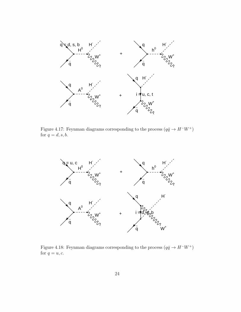
q = d, s, b

q−

H0H-

W+ +

q

q−

h0H-

W+

q

q−

A0H-

W+ +

q H-

i = u, c, t

q−

W+

Figure 4.17: Feynman diagrams corresponding to the process (qq → H−W+)for q = d, s, b.

q = u, c

q−

H0H-

W+ +

q

q−

h0H-

W+

q

q−

A0H-

W+ +

q

W+

i = d, s, b

q−

H-

Figure 4.18: Feynman diagrams corresponding to the process (qq → H−W+)for q = u, c.

24

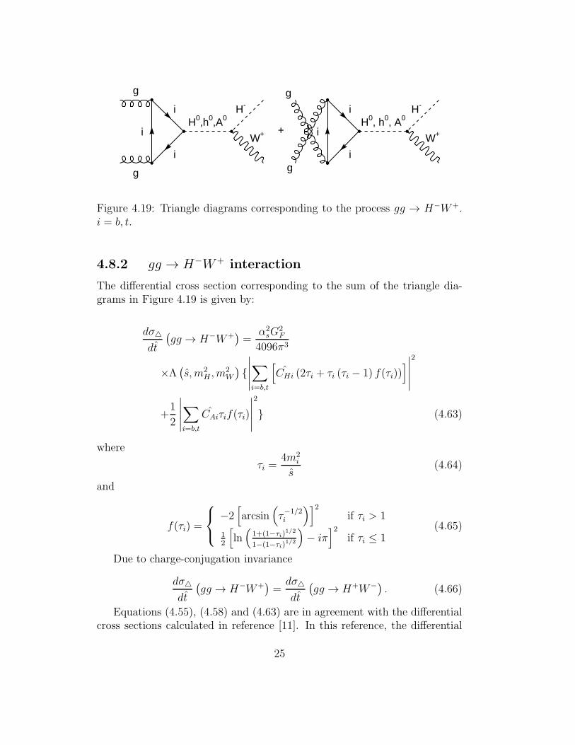
g

i

i

g

iH0,h0,A0

H-

W+ +

g

i

g

i

i

H0, h0, A0H-

W+

Figure 4.19: Triangle diagrams corresponding to the process gg → H−W+.i = b, t.

4.8.2 gg → H−W+ interaction

The differential cross section corresponding to the sum of the triangle dia-grams in Figure 4.19 is given by:

dσ

dt

(

gg → H−W+)

=α2sG

2F

4096π3

×Λ(

s, m2H , m

2W

)

∣

∣

∣

∣

∣

∑

i=b,t

[

CHi (2τi + τi (τi − 1) f(τi))]

∣

∣

∣

∣

∣

2

+1

2

∣

∣

∣

∣

∣

∑

i=b,t

CAiτif(τi)

∣

∣

∣

∣

∣

2

(4.63)

where

τi =4m2

i

s(4.64)

and

f(τi) =

−2[

arcsin(

τ−1/2i

)]2

if τi > 1

12

[

ln(

1+(1−τi)1/2

1−(1−τi)1/2

)

− iπ]2

if τi ≤ 1(4.65)

Due to charge-conjugation invariance

dσ

dt

(

gg → H−W+)

=dσ

dt

(

gg → H+W−) . (4.66)

Equations (4.55), (4.58) and (4.63) are in agreement with the differentialcross sections calculated in reference [11]. In this reference, the differential

25

cross section corresponding to the sum of the box diagrams of Figures 4.20and 4.21, also has been calculated with the aid of the computer packagesFEYNARTS, FEYNCALC and FF. According to the analisis presented in[11], the dominant subprocesses of W±H∓ associated production are bb →W±H∓ at the tree level and gg →W±H∓ at one loop.

4.8.3 Differential cross section pp→ H∓W±X

The differential cross section corresponding to the channel pp → H∓W±Xis:

d2σ

dyd (pT )2

(

pp→ H∓W±X)

=∑

f

∫ 1

xamin

dxaff(

xa, m2a

)

ff(

xb, m2b

)

× xbs

(m2H − u)

dσ

dt

(

f f → H∓W±) (4.67)

where f is q or g,

xamin =

√smT e

y +m2H −m2

W

s−√smT e−y, (4.68)

mT =(

m2W + p2T

)1

2 , (4.69)

xb =xa√smT e

−y +m2H −m2

W

xas−√smT ey

, (4.70)

s = xaxbs, (4.71)

p2T =Λ (s, m2

H , m2W ) sin2 θ

4s, (4.72)

u =1

2

(

m2H +m2

W − s− cos θΛ1/2(s, m2H , m

2W ))

, (4.73)

t =1

2

(

m2H +m2

W − s+ cos θΛ1/2(s, m2H , m

2W ))

, (4.74)

ut = m2Hm

2W + sp2T , (4.75)

and

cos θ =

(

1− 4sp2TΛ1/2(s, m2

H , m2W )

)1/2

(4.76)

26

g iH-

j

W+

ig

i +

g j

W+

i

H-

jg

j

g

i

g

iH-

j

W+

i

+

g

j

g

j

W+

i

H-

j

g i

W+

ig

jH-

j

+

gj

H-j

g

i

W+

i

g i

H-

ig

j

W+

j

+

gj

W+

j

g

i

H-

i

Figure 4.20: Box diagrams corresponding to the process gg → H−W+. i =d, s, b ; j = u, c, t. Continued in Figure 4.21.

27

g jH-

i

W+

jg

j +

g i

W+

j

H-

ig

i

g

j

g

jH-

i

W+

j

+

g

i

g

i

W+

j

H-

i

g j

W+

jg

iH-

i

+

gi

H-i

g

j

W+

j

g j

H-

jg

i

W+

i

+

gi

W+

i

g

j

H-

j

Figure 4.21: Continued from Figure 4.20.

28

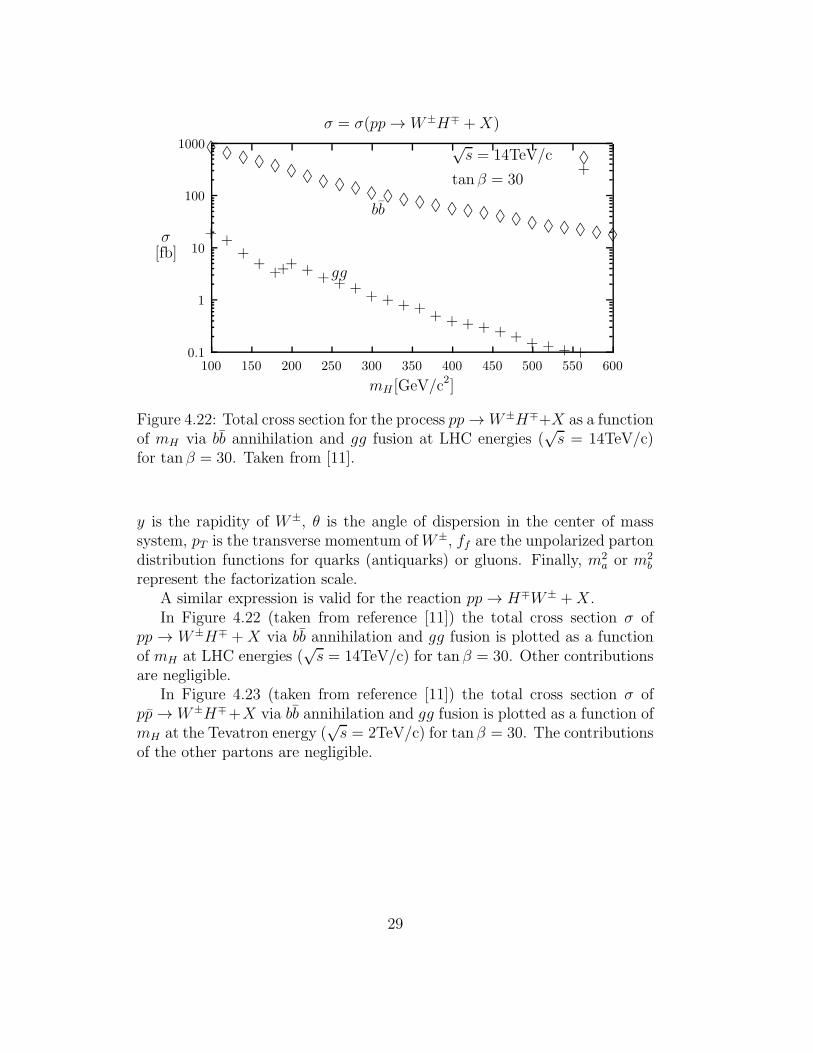
0.1

1

10

100

1000

100 150 200 250 300 350 400 450 500 550 600

σ[fb]

mH [GeV/c2]

σ = σ(pp→ W±H∓ +X)

√s = 14TeV/c

tan β = 30

bb

gg

♦ ♦ ♦ ♦ ♦ ♦ ♦ ♦ ♦ ♦ ♦ ♦ ♦ ♦ ♦ ♦ ♦ ♦ ♦ ♦ ♦ ♦ ♦ ♦ ♦ ♦

♦

+ ++

+++

+ + + + ++ + + + + + + + + + + + + +

+

Figure 4.22: Total cross section for the process pp→W±H∓+X as a functionof mH via bb annihilation and gg fusion at LHC energies (

√s = 14TeV/c)

for tan β = 30. Taken from [11].

y is the rapidity of W±, θ is the angle of dispersion in the center of masssystem, pT is the transverse momentum ofW±, ff are the unpolarized partondistribution functions for quarks (antiquarks) or gluons. Finally, m2

a or m2b

represent the factorization scale.A similar expression is valid for the reaction pp→ H∓W± +X .In Figure 4.22 (taken from reference [11]) the total cross section σ of

pp → W±H∓ +X via bb annihilation and gg fusion is plotted as a functionof mH at LHC energies (

√s = 14TeV/c) for tan β = 30. Other contributions

are negligible.In Figure 4.23 (taken from reference [11]) the total cross section σ of

pp→W±H∓+X via bb annihilation and gg fusion is plotted as a function ofmH at the Tevatron energy (

√s = 2TeV/c) for tanβ = 30. The contributions

of the other partons are negligible.

29

0.001

0.01

0.1

1

10

100 150 200 250 300

σ[fb]

mH [GeV/c2]

σ = σ(pp→ W±H∓ +X)

√s = 2TeV/ctan β = 30

bb

gg

♦♦♦♦♦♦♦♦♦♦♦♦♦♦♦♦♦♦♦♦♦♦♦♦♦♦♦♦♦♦♦♦♦♦♦♦♦♦♦♦♦

♦

+++++++++++++++++++++++++++++++++++++++++

+

Figure 4.23: Total cross section for the process pp → W±H∓ + X as afunction of mH via bb annihilation and gg fusion at the Tevatron energy(√s = 2TeV/c) for tanβ = 30. Taken from [11].

4.9 Comparison between µ−µ+ → H∓W± and

pp, pp→ H∓W±X for large values of tan β

Let us compare the channel µ−µ+ → H∓W± at√s = 500GeV/c with the

processes pp, pp → H∓W±X at the Tevatron energy (√s = 2TeV/c) and

LHC energies (√s = 14TeV/c) respectively for large values of tanβ (for

example tan β = 30).At the FNAL energy (Figure 4.24), we have: σ(µ−µ+ → H∓W±) >

σ(pp→W±H∓X) for tanβ = 30.At LHC energies (Figure 4.25), we have: σ(pp→W±H∓X) > σ(µ−µ+ →

H∓W±) for tan β = 30.According to Figure 4.12, σ(µ−µ+ → H∓W±) & 5fb for tan β ≥ 20 in

the mass interval 100 ≤ mH ≤ 400[GeV/c2], which would be an observablenumber ofH± for luminosities > 50fb−1. In the mass region of interest shownin the figures, the dominant decay mode of H± is H+ → tb or H− → tb.So the main background would be from tt production. Reference [4] showsthat such a background overwhelms the charged Higgs boson signal in pp→W±H∓X at the LHC. In fact, in Section 4.7 we have shown that σ(µ−µ+ →tt) ≈ 495fb for

√s = 500GeV/c. In the LHC the background due to tt

30

0.001

0.01

0.1

1

10

100

100 150 200 250 300 350 400 450

σ[fb]

mH [GeV/c2]

µ−µ+ → H∓W± and pp→W±H∓X

tan β = 30

µ−µ+ → H∓W±

bb

gg pp→W±H∓X

♦♦♦♦♦♦♦♦♦♦♦♦♦♦♦♦♦♦♦♦♦♦♦♦♦♦♦♦♦♦♦♦♦♦♦♦♦♦♦♦♦

♦

+++++++++++++++++++++++++++++++++++++++++

+

Figure 4.24: Total cross section for the processes µ−µ+ → H∓W± and pp→W±H∓ + X (via bb annihilation and gg fusion) as a function of mH at√s = 500GeV/c and

√s = 2TeV/c, respectively, for tanβ = 30. Taken

partially from [11].

production is of order [4] 800 pb (three orders of magnitude larger than at amuon collider with

√s = 500GeV/c). At the FNAL energy (

√s = 2TeV/c)

something similar happens because σ(pp→ tt) = 5.5pb [12].In the muon collider, the signal of the charged Higgs boson is not over-

whelmed.Then, for large values of tanβ, the process µ−µ+ → H∓W± is a very

attractive channel for the search of H± at a µ−µ+ collider.

4.10 Conclusions

The discovery of the Standard Model Higgs is one of the principal goals ofexperimental and theoretical particle physicists. This is because the Higgsmechanism is a cornerstone of the Standard Model. The search for the Stan-dard Model Higgs will also constrain or discover particles of the Two HiggsDoublet Model of type II.

In this paper we have discussed the masses of the Higgs particles in theTwo Higgs Doublet Model of type II, and considered the influence of theradiative corrections on these masses. In the absence of radiative corrections,

31

0.1

1

10

100

1000

100 150 200 250 300 350 400 450 500 550 600

σ[fb]

mH [GeV/c2]

µ−µ+ → H∓W± and pp→W±H∓X

tan β = 30bb

pp→W±H∓X

µ−µ+ → H∓W±

gg

♦ ♦ ♦ ♦ ♦ ♦ ♦ ♦ ♦ ♦ ♦ ♦ ♦ ♦ ♦ ♦ ♦ ♦ ♦ ♦ ♦ ♦ ♦ ♦ ♦ ♦

♦

+ ++

+++

+ + + + ++ + + + + + + + + + + + + +

+

Figure 4.25: Total cross section for the processes µ−µ+ → H∓W± and pp→W±H∓ + X (via bb annihilation and gg fusion) as a function of mH at√s = 500GeV/c and

√s = 14TeV/c, respectively, for tan β = 30. Taken

partially from [11].

32

the Higgs boson h0 obeys the bound mh0 ≤ mZ . This bound practicallyhas been excluded by the present limits on mh0 obtained by LEP and CDF[6]. However, when the radiative corrections are taken into account, mh0

increases as the value of mA increases. As a result, we have a new bound:mh0 ≤ 128.062GeV/c2 taking Msb (sbottom mass) and Mst (stop mass) oforder 1TeV/c2.

Considering the radiative corrections of the masses, we have calculatedHiggs production cross sections at a muon collider in the Two Higgs DoubletModel of type II. The most interesting production channels are µ−µ+ →h0Z0, H0Z0 , H−H+, A0Z0 and H∓W±. In the first two channels the radia-tive corrections of the masses play an important role, which is not true forthe other channels. In the reaction µ−µ+ → h0Z0, the total cross sectionbecomes important in the mass interval 118 ≤ mh0 ≤ 128[GeV/c2].

The process µ−µ+ → A0Z0, would provide an alternative way for search-ing the A0 looking for peaks in the bb distribution. Another interestingchannel could be µ−µ+ → A0h0. However, this is highly supressed formA ≥ 200GeV/c2 because the total cross section is proportional to the factor

cos2 (β − α) = (1 + tanβ tanα)2

(1 + tan2 β) (1 + tan2 α)

(see the Feynman rules given in [9]). This factor decreases as the mass of theA0 increases.

The most attractive channel is µ−µ+ → H∓W±, see Figures 4.24 and4.25. In this reaction σ(µ−µ+ → H∓W±) & 5fb for tan β ≥ 20 in the massinterval 100 ≤ mH ≤ 400[GeV/c2], which would give an observable numberof H± for luminosities > 50fb−1 at

√s = 500GeV/c.

Because the main background in a hadron collider in the reactions pp→W±H∓X (Tevatron energy) or pp → W±H∓X (LHC energies) comes fromtt production, the charged Higgs boson signal would be overwhelmed by sucha background. In a muon collider with

√s = 500GeV/c, the signal of the H±

is not overwhelmed. This means, that for large values of tanβ, the channelµ−µ+ → H∓W± is a very attractive channel for the search of charged Higgsbosons at a µ−µ+ collider.

Acknowledgment

I would like to thank Bruce Hoeneisen for the critical reading of thismanuscript.

33

Bibliography

[1] Bruce Hoeneisen, Serie de Documentos USFQ 26, Universidad San Fran-cisco de Quito, Ecuador (2001).

[2] J. Gunion, hep-ph/9802258; V. Barger, hep-ph/9803480.

[3] A. G. Akeroyd, A. Arhrib, C. Dove, Phys. Rev. D 61, 071702 (2000).

[4] Stefano Moretti, Kosuke Odagiri, Phys. Rev. D 59, 055008 (1999).

[5] Vernon Barger and Roger Phillips, Collider Physics (Addison Wesley,1988); S. Dawson, J.F. Gunion, H.E. Haber and G. Kane, The HiggsHunter’s Guide (Addison Wesley, 1990).

[6] Review of Particle Physics, K. Hagiwara et al., Phys. Rev. D 66, 010001(2002).

[7] ”The quantum theory of fields”, Volume III, Supersymmetry, StevenWeinberg, Cambridge University Press (2000).

[8] Zhou Fei et al., Phys. Rev. D 64, 055005(2001).

[9] C. Marın and B. Hoeneisen, hep-ph/0402061 v1 (2004).

[10] C. Marın, Politecnica, XVII No. 1, p.79 (1992), Escuela PolitecnicaNacional, Quito, Ecuador. DO Note Fermilab (1992).

[11] A. A. Barrientos Bendezu and B. A. Kniehl, Phys. Rev. D 59, 015009(1998).

[12] V. M. Abazov et al., Phys. Rev. Lett. 88, 151803 (2002).

34

Appendix A

Functions SWW , SHW and SHH

If i 6= j:

SWW(

xiW , xjW

)

=xiW + xjW − 11

4xiWx

jW

(1− xiW )(

1− xjW)

+1

(

xiW − xjW)

[

G(

xiW , xjW

)

−G(

xjW , xiW

)]

(A.1)

where

G(

xiW , xjW

)

=(xiW )

2ln (xiW )

(1− xiW )2

[

1− 2xjW +1

4xiWx

jW

]

. (A.2)

If i = j:

SWW(

xiW , xiW

)

=xiW

(1− xiW )2

[

3− 19

4xiW +

1

4

(

xiW)2]

+2xiW ln (xiW )

(1− xiW )2

[

1− 3

4

(xiW )2

(1− xiW )

]

. (A.3)

If i 6= j:

SHH(

xiH , xjH , x

WH

)

=xiHx

jH

xWH

[

J (xiH)− J(

xjH)

xiH − xjH

]

(A.4)

with

J(

xiH)

=1

(1− xiH)+

(xiH)2ln (xiH)

(1− xiH)2 . (A.5)

If i = j:

SHH(

xiH , xiH , x

WH

)

=(xiH)

2

xWH

[

1− (xiH)2+ 2xiH ln (xiH)

(1− xiH)3

]

. (A.6)

1

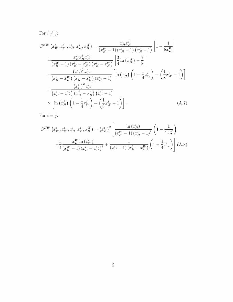
For i 6= j:

SHW(

xiW , xjW , x

iH , x

jH , x

WH

)

=xiHx

jH

(xWH − 1) (xiH − 1)(

xjH − 1)

[

1− 1

8xWH

]

+xiHx

jHx

WH

(xWH − 1) (xiH − xWH )(

xjH − xWH)

[

3

4ln(

xWH)

− 7

8

]

+(xiH)

2xjH

(xiH − xWH )(

xiH − xjH)

(xiH − 1)

[

ln(

xiH)

(

1− 1

4xiW

)

+

(

1

8xiW − 1

)]

+

(

xjH)2xiH

(

xjH − xWH) (

xjH − xiH) (

xjH − 1)

×[

ln(

xjH)

(

1− 1

4xjW

)

+

(

1

8xjW − 1

)]

. (A.7)

For i = j:

SHW(

xiW , xiW , x

iH , x

iH , x

WH

)

=(

xiH)2

[

ln (xiH)

(xWH − 1) (xiH − 1)2

(

1− 1

4xWH

)

−34

xWH ln (xiW )

(xWH − 1) (xiH − xWH )2 +

1

(xiH − 1) (xiH − xWH )

(

1− 1

4xiW

)

]

.(A.8)

2

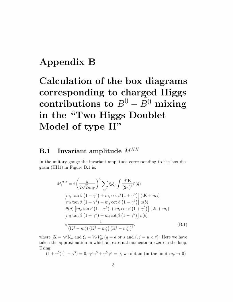
Appendix B

Calculation of the box diagrams

corresponding to charged Higgs

contributions to B0 − B0 mixing

in the “Two Higgs Doublet

Model of type II”

B.1 Invariant amplitude MHH

In the unitary gauge the invariant amplitude corresponding to the box dia-gram (HH1) in Figure B.1 is:

MHH1 = i

(

g

2√2mW

)4∑

i,j

ξiξj

∫

d4K

(2π)4v(q)

[

mq tan β(

1− γ5)

+mj cotβ(

1 + γ5)]

( 6 K+mj)[

mb tan β(

1 + γ5)

+mj cot β(

1− γ5)]

u(b)

·u(q)[

mq tanβ(

1− γ5)

+mi cotβ(

1 + γ5)]

( 6 K+mi)[

mb tan β(

1 + γ5)

+mi cot β(

1− γ5)]

v(b)

× 1

(K2 −m2i )(

K2 −m2j

)

(K2 −m2H)

2 . (B.1)

where 6 K = γµKµ and ξi = VibV∗iq (q = d or s and i, j = u, c, t). Here we have

taken the approximation in which all external momenta are zero in the loop.Using:

(1 + γ5) (1− γ5) = 0, γµγ5 + γ5γµ = 0, we obtain (in the limit mq → 0)

3

b− µ, W+/- µ q

−

j

ν bW+/-q

i

ν,

(WW1)

b− µ, j µ q

−

W+/-

bνiq ν,

W+/-

(WW2)

b−

H+/- q−

j

bH+/-q

i

(HH1)

b−

j q−

H+/-

biq

H+/-

(HH2)

b−

ν W+/- µ q−

j

bH+/-q

i

(HW1)

b−

j µ q−

W+/-

bνiq

H+/-

(HW2)

b−

H+/- q−

j

ν bW+/-q

i

µ(HW3)

b− ν j q

−

H+/-

biµq

W+/-

(HW4)

Figure B.1: Feynman diagrams corresponding to Bo ↔ Bo mixing in theTwo Higgs Doublet Model. q = d or s and i, j = u, c, t. The diagrams onthe right side interfer with a “-” sign.

4

MHH1 = 4i

(

g

2√2mW

)4∑

i,j

ξiξjm2im

2j cot

4 βv(q)γα(

1− γ5)

u(b)

·u(q)γβ(

1− γ5)

v(b)IHHαβ (i, j) +m2

im2jm

2b v(q)

(

1 + γ5)

u(b)

·u(q)(

1 + γ5)

v(b)IHH(i, j) +m2im

2jmb cot

2 βv(q)(

γα(

1− γ5)

u(b) · u(q)(

1 + γ5)

+(

1 + γ5)

u(b) · u(q)γα(

1− γ5))

v(b)IHHα (i, j) (B.2)

where

IHHαβ (i, j) ≡

∫

d4K

(2π)4KαKβ

(K2 −m2H)

2(K2 −m2

i )(

K2 −m2j

) (B.3)

IHHα (i, j) ≡

∫

d4K

(2π)4Kα

(K2 −m2H)

2(K2 −m2

i )(

K2 −m2j

) (B.4)

IHH(i, j) ≡∫

d4K

(2π)41

(K2 −m2H)

2(K2 −m2

i )(

K2 −m2j

) (B.5)

The integrals, IHHαβ (i, j) and IHH(i, j), were calculated in detail in Appendix

2 of reference [1] (replacing mH by mW ):If i 6= j:

IHHαβ (i, j) =

−iπ2ηαβ

4 (2π)4m2H

[

J (xiH)− J(

xjH)

xiH − xjH

]

(B.6)

whereηαβ = diag(1,−1,−1,−1),

xiH =m2

i

m2H

and J (xiH) is given in Equation A.5.

If i = j:

IHHαβ (i, i) =

−iπ2ηαβ

4 (2π)4m2H

[

1− (xiH)2+ 2xiH ln (x

iH)

(1− xiH)3

]

. (B.7)

If i 6= j:

IHH(i, j) =iπ2

(2π)4m4H

1

(1− xiH)(

1− xjH)

[

F(

xiH , xjH

)

+ F(

xjH , xiH

)

− 1]

(B.8)

5

where

F(

xiH , xjH

)

= − xiH ln (x

iH)(

1− xjH)

(1− xiH)(

xiH − xjH) . (B.9)

If i = j:

IHH(i, i) =−iπ2

(2π)4m4H

1

(1− xiH)2

[

2 +(1 + xiH)

(1− xiH)ln(

xiH)

]

. (B.10)

The value of the second integral (see Appendix C) is:For i 6= j and i = j:

IHHα (i, j) = 0. (B.11)

Neglecting the second term in (B.2) and because GF√2= g2

8m2W, we have

MHH1 =

G2Fm

2W

32π2cot4 β

∑

i,j

ξiξj v(q)γµ(

1− γ5)

u(b)

·u(q)γµ(

1− γ5)

v(b)SHH(

xiH , xjH , x

WH

)

. (B.12)

SHH(

xiH , xjH , x

WH

)

for i 6= j and i = j are given in (A.4) and (A.6), respec-tively.Note that:

limxiH→0

SHH(

xiH , xiH , x

WH

)

= 0. (B.13)

In a similar way, we can chow that the invariant amplitude correspondingto the diagram (HH2) in Figure B.1 is:

MHH2 =

G2Fm

2W

32π2cot4 β

∑

i,j

ξiξj v(q)γµ(

1− γ5)

v(b)

·u(q)γµ(

1− γ5)

u(b)SHH(

xiH , xjH , x

WH

)

. (B.14)

According to the Fierz Theorem [2], we can write

v(q)γµ(

1− γ5)

v(b) · u(q)γµ(

1− γ5)

u(b)

= −v(q)γµ(

1− γ5)

u(b) · u(q) γµ(

1− γ5)

v(b) (B.15)

The total amplitude MHH is then

MHH = 2MHH1 . (B.16)

6

Let’s consider the amplitude:

〈B0|MHH |B0〉 = G2Fm

2W

4π2cot4 β

∑

i,j

ξiξjASHH(xiH , x

jH , x

WH ) (B.17)

where

A ≡ 〈B0|vL(q)γµuL(b) · uL(q)γµvL(b)|B0〉,

vL(q)γµ = v(q)γµ

1

2

(

1− γ5)

,

vL(b) =1

2

(

1− γ5)

v(b),

uL(q)γµ = u(q)γµ1

2

(

1− γ5)

,

uL(b) =1

2

(

1− γ5)

u(b),

For our model, ‘free particles inside the meson” [1], we have

A =1

16βBf

2BmB (B.18)

Thus, one obtains

〈B0|MHH |B0〉 = βBG2Fm

2W f

2BmB

64π2cot4 β

∑

i,j

ξiξjSHH(xiH , x

jH , x

WH ) (B.19)

B.2 Invariant amplitude MHW

For the box diagram (HW1) of Figure B.1, the corresponding invariant am-plitude is given by:

MHW1 = −i

(

g

2√2

)41

m2W

∑

i,j

ξiξj

∫

d4K

(2π)4v(q)γµ

(

1− γ5)

( 6 K+mj)[

mb tanβ(

1 + γ5)

+mj cotβ(

1− γ5)]

u(b)

·u(q)[

mq tanβ(

1− γ5)

+mi cot β(

1 + γ5)]

( 6 K+mi) γν(

1− γ5)

v(b)

(

ηµν −KµKν

m2W

)

× 1

(K2 −m2W ) (K2 −m2

H) (K2 −m2

i )(

K2 −m2j

) (B.20)

7

Using:γµγ5 + γ5γµ = 0 , (1 + γ5)

2= 2 (1 + γ5) , (1− γ5)2 = 2 (1− γ5) ,

6 K 6 K = K2, and taking the limit in which mq → 0, we can write the invariantamplitude as

MHW1 = −4i

(

g

2√2

)41

m2W

∑

i,j

ξiξjm2im

2j cot

2 βv(q)γα(

1− γ5)

u(b)

·u(q)(

γαIHW (i, j)− 1

m2W

γβIHWαβ (i, j)

)

(

1− γ5)

v(b)

+m2imbv(q)γ

µ(

1− γ5)

γαu(b) · u(q)γµ(

1− γ5)

v(b)(

IHWα

)(1)(i, j)

− 1

m2W

m2imbv(q)

(

1 + γ5)

u(b)

·u(q)γα(

1− γ5)

v(b)(

IHWα

)(2)(i, j) (B.21)

where

IHW (i, j) ≡∫

d4K

(2π)41

(K2 −m2W ) (K2 −m2

H) (K2 −m2

i )(

K2 −m2j

) (B.22)

IHWαβ (i, j) ≡

∫

d4K

(2π)4KαKβ

(K2 −m2W ) (K2 −m2

H) (K2 −m2

i )(

K2 −m2j

) (B.23)

(

IHWα

)(1)(i, j) ≡

∫

d4K

(2π)4Kα

(K2 −m2W ) (K2 −m2

H) (K2 −m2

i )(

K2 −m2j

)

(B.24)

(

IHWα

)(2)(i, j) ≡

∫

d4K

(2π)4K2Kα

(K2 −m2W ) (K2 −m2

H) (K2 −m2

i )(

K2 −m2j

)

(B.25)After momentum integration (see Appendix C), we get

8

If i 6= j:

IHW (i, j) =−iπ2

(2π)41

m4H

1

(xWH − 1)

×[

xWH(

ln(

xWH)

− 1)

(xiH − xWH )(

xjH − xWH) +

1

(xiH − 1)(

xjH − 1)

+

(

xWH − 1)

(

xjH − xWH) (

xjH − xiH) (

xjH − 1)xjH

(

ln(

xjH)

− 1)

+

(

xWH − 1)

(xiH − xWH )(

xiH − xjH

)

(xiH − 1)xiH(

ln(

xiH)

− 1)

]

(B.26)

If i = j:

IHW (i, i) =−iπ2

(2π)41

m4H

1

(xWH − 1)

[

xWH(

ln(

xWH)

− 1)

(xiH − xWH )2 +

1

(xiH − 1)2

+

(

xWH − 1)

[

ln (xiH)(

xWH − (xiH)2)

+ xiH(

2xiH − xWH − 1)

]

(xiH − xWH )2(xiH − 1)

2

(B.27)

If i 6= j:

IHWαβ (i, j) =

−iπ2

8 (2π)4ηαβ

1

m2H

1

(xWH − 1)

×[

−(

xWH − 1)

(xiH)2(2ln (xiH)− 1)

(

xjH − xiH)

(xiH − 1) (xiH − xWH )

−(

xWH − 1) (

xjH)2 (

2ln(

xjH)

− 1)

(

xiH − xjH) (

xjH − 1) (

xjH − xWH)

+1

(xiH − 1)(

xjH − 1) +

(

xWH)2 (

2ln(

xWH)

− 1)

(xiH − xWH )(

xjH − xWH)

]

(B.28)

If i = j:

IHWαβ (i, i) =

−iπ2

8 (2π)4ηαβ

1

m2H

1

(xWH − 1)

[

(

xWH − 1)

(xiH)

(xiH − 1)2(xiH − xWH )

2

×[

xiH(

2xiH − xWH − 1)

− 2ln(

xiH) (

xiHxWH + xiH − 2xWH

)]

+1

(xiH − 1)2 +

(

xWH)2 (

2ln(

xWH)

− 1)

(xiH − xWH )2

]

(B.29)

9

For i 6= j and i = j:(

IHWα

)(1)(i, j) = 0 (B.30)

For i 6= j and i = j:(

IHWα

)(2)(i, j) = 0 (B.31)

Introducing these integrals in B.21, we find

MHW1 = −G

2Fm

2W cot2 β

8π2

∑

i,j

ξiξj v (q) γµ(

1− γ5)

u(b)

·u (q) γµ(

1− γ5)

v(

b)

SHW(

xiW , xjW , x

iH , x

jH , x

WH

)

(B.32)

where SHW(

xiW , xjW , x

iH , x

jH , x

WH

)

is given in (A.7) and (A.8).Note that

limxiH→0

SHW(

xiW , xiW , x

iH , x

iH , x

WH

)

= 0. (B.33)

We have another three diagrams. In the limit mq → 0, the Fierz transfor-mation shows that all four diagrams contribute equally and then, the totalinvariant amplitude is:

MHW = 4MHW1 (B.34)

Therefore, as in (B.19), the matrix element 〈B0|MHW |B0〉 can be expressedas

〈B0|MHW |B0〉 = −βBG2Fm

2W f

2BmB

8π2cot2 β

∑

i,j

ξiξjSHW

(

xiW , xjW , x

iH , x

jH , x

WH

)

. (B.35)

B.3 Invariant amplitude MWW

The calculation of the invariant amplitude for the box diagrams (WW) inFigure B.1, was performed in detail in reference [1]:

MWW =G2

Fm2W

π2

∑

i,j

ξiξj vL(q)γµuL(b) · uL(q)γµvL(b)SWW (xiW , x

jW ) (B.36)

10

Therefore

〈B0|MWW |B0〉 = βBG2Fm

2W f

2BmB

16π2

∑

i,j

ξiξjSWW

(

xiW , xjW

)

. (B.37)

B.4 Mass difference ∆mB

The mass difference between the two states that diagonalize the hamiltonianis:

∆mB = mBH−mBL

= 2|M12| = 2|〈B0|MHH +MHW +MWW |B0〉|= 2|〈B0|MHH |B0〉+ 〈B0|MHW |B0〉+ 〈B0|MWW |B0〉| (B.38)

where H and L stand for Heavy and Light, repectively.Introducing (B.19), (B.35), and (B.37) in Equation (B.38) (after correctingby a color factor 4/3), we arrive to Equation (2.4).

11

Appendix C

Integrals

C.1 IHHα (i, j)

From the identity:

1

abcd= 3!

∫ 1

0

∫ 1

0

∫ 1

0

x2ydxdydz

[(1− x) d+ x (1− y) c+ xy (1− z) b+ xyza]4(C.1)

where a, b, c, d 6= 0; and setting:a = (K2 −m2

H), b = (K2 −m2H), c = (K2 −m2

i ), d =(

K2 −m2j

)

,it is found that

1

(K2 −m2H)

2(K2 −m2

i )(

K2 −m2j

)

= 3!

∫ 1

0

∫ 1

0

∫ 1

0

x2ydxdydz[

K2 + x(

m2j −m2

i

)

+ xy (m2i −m2

H)−m2j

]4 (C.2)

Introducing the last Equation in (B.4), we obtain

IHHα (i, j) = 3!

∫ 1

0

∫ 1

0

∫ 1

0

dxdydzx2y

∫

d4K

(2π)4Kα

[K2 +M2]4(C.3)

whereM2 = x

(

m2j −m2

i

)

+ xy(

m2i −m2

H

)

−m2j (C.4)

Then using [3]

Iµ =

∫

ddK

(2π)dKµ

(K2 + 2P ·K+M2 + iǫ)α= −PµI0 (C.5)

12

I0 =

∫

ddK

(2π)d1

(K2 + 2P ·K+M2 + iǫ)α

=i (−π)d/2

(2π)dΓ(

α− d2

)

Γ (α)

1

(M2 − P 2 + iǫ)α−d2

(C.6)

With n = 4, α = 4 and Pµ = 0, we get

IHHα (i, j) = 0. (C.7)

C.2(

IHWα

)(1)(i, j)

Again, using the identity (C.1) for:a = (K2 −m2

H), b = (K2 −m2W ), c = (K2 −m2

i ), d =(

K2 −m2j

)

,we obtain the same integral (C.7), but with

M2 = x(

m2j −m2

i

)

+ xy(

m2i −m2

W

)

+ xyz(

m2W −m2

H

)

−m2j (C.8)

Once more, (C.5) implies

(

IHWα

)(1)(i, j) = 0. (C.9)

C.3(

IHWα

)(2)(i, j)

On account of (C.1), we can write

(

IHWα

)(2)(i, j) = 3!γµγν

∫ 1

0

∫ 1

0

∫ 1

0

dxdydzx2y

∫

d4K

(2π)4KµKνKα

[K2 +M2]4(C.10)

then, from [3]

Iµνα =

∫

ddK

(2π)dKµKνKα

[K2 + 2P ·K+M2 + iǫ]α

= −I0[

PµPνPα +(M2 − P 2)

2(

α− d2− 1) (ηµνPα + ηµαPν + ηναPµ)

]

(C.11)

With n = 4, α = 4 and Pµ = 0, we get

(

IHWα

)(2)(i, j) = 0. (C.12)

13

C.4 IHW (i, j)

Equation (B.22) can be written as:

IHW (i, j) = 3!

∫ 1

0

∫ 1

0

∫ 1

0

dxdydzx2y

∫

d4K

(2π)41

(K2 +M2)4(C.13)

From (C.6), we have

∫

d4K

(2π)41

(K2 +M2)4=

iπ2

(2π)41

3! (M2)2(C.14)

and then

IHW (i, j) =iπ2

(2π)4

∫ 1

0

∫ 1

0

∫ 1

0

f(x, y, z)dxdydz (C.15)

where

f(x, y, z) =x2y

[

x(

m2j −m2

i

)

+ xy (m2i −m2

W ) + xyz (m2W −m2

H)−m2j

]2

(C.16)Integrating (C.15), we obtain (B.26) and (B.27).

C.5 IHWαβ (i, j)

Equation (B.23) can be written as:

IHWαβ (i, j) = 3!

∫ 1

0

∫ 1

0

∫ 1

0

dxdydzx2y

∫

d4K

(2π)4KαKβ

(K2 +M2)4(C.17)

Using the integral [3]

Iαβ =

∫

ddK

(2π)dKαKβ

(K2 + 2P ·K+M2 + iǫ)α

= I0

[

PαPβ +1

2ηαβ(

M2 − P 2) 1(

α− d2− 1)

]

, (C.18)

we obtain

∫

d4K

(2π)4KαKβ

(K2 +M2)4=

iπ2

2 (2π)41

3!M2ηαβ (C.19)

14

and therefore, (C.17) becomes

IHWαβ (i, j) =

iπ2

2 (2π)4ηαβ

∫ 1

0

∫ 1

0

∫ 1

0

g(x, y, z)dxdydz (C.20)

where

g(x, y, z) =x2y

[

x(

m2j −m2

i

)

+ xy (m2i −m2

W ) + xyz (m2W −m2

H)−m2j

]

(C.21)After some long, but trivial calculations, we arrive to Equations (B.28) and(B.29).

15

Appendix D

A0→ Z0γ decay

As an example, we derive the expression for the width decay correspondingto the channel A0 → Z0γ. The Feynman diagrams are given in Figure D.1.

D.1 (a) i = e−, µ−, τ−, d, s, b

In the unitary gauge, the invariant amplitude corresponding to the first Feyn-man diagram of Figure D.1 is:

M1a = −g2e tanβ

4mW cos θW

∑

i=d,s,b,..

NiQimi

∫

ddK

(2π)d(T )

× 1

(K2 −m2i )[

(K− P2)2 −m2

i

] [

(K + P1)2 −m2

i

]ǫ∗1µǫ∗2νµ

∗ (D.1)

where

T = Trace[

γµ(

giV − giAγ5)

( 6 K+mi) γν ( 6 K− 6 P2 +mi) γ

5 ( 6 K+ 6 P1 +mi)]

(D.2)and µ∗ = µ(4−d)/2 is a mass parameter. Qi and mi are the charge and massof the particle i, and Ni is a color factor (Ni = 1 for leptons, Ni = 3 forquarks). P1 and P2 are the momenta of the Z0 and the photon, respectively.Finally, ǫ∗1µ and ǫ∗2ν are polarization vectors.Using

γµγ5 + γ5γµ = 0, (D.3)

γµ 6 K+ 6 Kγµ = 2Kµ, (D.4)

16

A0 i

Z0 1µ

iK

γ 2ν

i

+

A0 i

γ

ν 2

iK

Z0

µ 1

i

Figure D.1: Feynman diagrams corresponding to the decay A0 → Z0γ. i =d, s, b, e−, µ−, τ− or u, c, t.

17

trace(odd number of γ′

s) = 0, (D.5)

trace (γµγν) = dηµν , (D.6)

trace (γµγνγργσ) = d (ηµνηρσ − ηµρηνσ + ηµσηνρ) , (D.7)

trace(

γ5γµγνγαγβ)

= −4iǫµναβ , (D.8)

trace(

γ5γµγν)

= 0, (D.9)

and

6 K 6 K = K2, (D.10)

we can show that

T = dmi−2giAP µ1 K

ν − 4i

dgiV ǫ

µναβP2αP1β

+giA [−2KνPµ2 + 2 (P2 ·K) ηµν ]− giAK2ηµν

+giA (ηµν (P1 · P2)− Pµ2P

ν1 + Pµ

1Pν2) +m2

i giAη

µν (D.11)

From the identity [4]

1

abc= 2

∫ 1

0

dx

∫ 1−x

0

dy

[a (1− x− y) + bx+ cy]3(D.12)

where a, b, c 6= 0; and setting:a = (K2 −m2

i ), b =[

(K + P1)2 −m2

i

]

, c =[

(K− P2)2 −m2

i

]

,we have

1

(K2 −m2i )[

(K + P1)2 −m2

i

] [

(K− P2)2 −m2

i

]

= 2

∫ 1

0

dx

∫ 1−x

0

dy

[K2 −m2i +m2

Zx+ 2K · (P1x− P2y)]3 (D.13)

putting K′

= K+ (P1x− P2y), and working in the rest frame of A0, we get

18

M1a = −2g2e tan βd

4mW cos θW

∑

i=d,s,b,...

NiQim2i

∫ 1

0

dx

∫ 1−x

0

dy

∫

ddK′

(2π)d−2giAPµ

1K′ν − 4i

dgiV ǫ

µναβP2αP1β − 2giAPµ2K

′ν

+2giAηµν(

P2 ·(

K′ − (P1x− P2y)

))

− giAηµν(

K′ − (P1x− P2y)

)2

+giAηµν (P1 · P2) +m2

i giAη

µν

×[

K′2 −m2

i +m2Zx−m2

Zx2 + 2 (P1 · P2)xy

]−3

ǫ∗1µǫ∗2νµ

∗ (D.14)

where we have used: Pµ1ǫ

∗2µ = 0, Pµ

1ǫ∗1µ = 0 and Pν

2ǫ∗2ν = 0.

With the integrals [3]:

∫

ddK′ K

′µ

[K′2 −m2i +m2

Zx (1− x) + 2 (P1 · P2) xy]3 = 0, (D.15)

∫

ddK′ 1

[K′2 −m2i +m2

Zx (1− x) + 2 (P1 · P2)xy]3 = I0 (x, y) , (D.16)

and

∫

ddK′ K

′2

[K′2 −m2i +m2

Zx (1− x) + 2 (P1 · P2) xy]3

= I0 (x, y)d

2

[−m2i +m2

Zx (1− x) + 2 (P1 · P2) xy](

2− d2

) (D.17)

where

I0 (x, y) =i (−π)d/2 Γ

(

3− d2

)

2 [−m2i +m2

Zx (1− x) + 2 (P1 · P2)xy]3−d/2

; (D.18)

we get

19

M1a = −2g2e tan βd

4mW cos θW (2π)d

∑

i=d,s,b,...

NiQim2i

∫ 1

0

dx

∫ 1−x

0

dyI0 (x, y)

×[

−4idgiV ǫ

µναβP2αP1β − 2giAηµν (P1 · P2)x+ giAη

µν (P1 · P2)

+m2i g

iAη

µν − giAηµνm2Zx

2 + 2 (P1 · P2) xygiAη

µν

−giAηµνd

2

[−m2i +m2

Zx (1− x) + 2 (P1 · P2)xy](

2− d2

)

]

ǫ∗1µǫ∗2νµ

∗ (D.19)

The invariant amplitude corresponding to the second Feynman diagramof Figure D.1 (crossed diagram) is:

M2a = −g2e tanβ

4mW cos θW

∑

i=d,s,b,...

NiQimi

∫

ddK

(2π)d(Tra)

× 1

(K2 −m2i )[

(K− P1)2 −m2

i

] [

(K + P2)2 −m2

i

]ǫ∗1µǫ∗2νµ

∗ (D.20)

where

Tra = Trace[

γν ( 6 K+mi) γµ(

giV − giAγ5)

[( 6 K− 6 P1) +mi] γ5 [( 6 K+ 6 P2) +mi]

]

(D.21)

In a similar way, and after performing the calculation of the trace, we canshow that

M2a = −2g2e tan βd

4mW cos θW (2π)d

∑

i=d,s,b,...

NiQim2i

∫ 1

0

dx

∫ 1−x

0

dyI0 (x, y)

×[

−4idgiV ǫ

νµαβP1αP2β + 2giAηµν (P1 · P2) x− giAηµν (P1 · P2)

−m2i g

iAη

µν + giAηµνm2

Zx2 − 2 (P1 · P2) xyg

iAη

µν

+giAηµν d

2

[−m2i +m2

Zx (1− x) + 2 (P1 · P2)xy](

2− d2

)

]

ǫ∗1µǫ∗2νµ

∗ (D.22)

Adding Equations (D.19) and (D.22), we obtain

20

M1a +M2a =4ig2e tanβ

mW cos θW (2π)dǫµναβP2αP1β

∑

i=d,s,b,...

NiQim2i g

iV

∫ 1

0

dx

∫ 1−x

0

dyI0 (x, y) ǫ∗1µǫ

∗2νµ

∗ (D.23)

In the limit d→ 4, I0 (x, y) is

I0 (x, y) =iπ2

2

1

[−m2i +m2

Zx (1− x) + 2 (P1 · P2)xy](D.24)

Introducing

Ii =

∫ 1

0

dx

∫ 1−x

0

1

[−m2i +m2

Zx (1− x) + 2 (P1 · P2) xy]dy, (D.25)

we can write

M1a +M2a =g2e tanβ

8π2mW cos θWǫµναβP1αP2β

(

∑

i=d,s,b,...

NiQim2i g

iV Ii

)

ǫ∗1µǫ∗2ν (D.26)

D.2 b) i = u, c, t

In this case, the invariant amplitude is obtained from Equation (D.26) re-placing tan β by cot β, and then

M1b +M2b =g2e cot β

8π2mW cos θWǫµναβP1αP2β

(

∑

i=u,c,t

NiQim2i g

iV Ii

)

ǫ∗1µǫ∗2ν (D.27)

D.3 Width decay

The total invariant amplitude corresponding to the process A0 → Z0γ is

M =M1a+M2a+M1b+M2b =g2e

8π2mW cos θWǫµναβP1αP2βǫ

∗1µǫ

∗2νL(β) (D.28)

21

where

L(β) = tan β∑

i=d,s,b,...

NiQim2i g

iV Ii + cotβ

∑

i=u,c,t

NiQim2i g

iV Ii (D.29)

The absolute value of the invariant amplitude squared and summed over finalpolarizations is

|M |2 = g4e2

64π4m2W cos2 θW

ǫµναβǫρσγδP1αP2βP1γP2δ

(

∑

λ

ǫ1µǫ∗1ρ

)

∑

λ′

ǫ2νǫ∗2σ

|L(β)|2 (D.30)

Since∑

λ

ǫ1µǫ∗1ρ = −ηµρ +

P1µP1ρ

m2Z

, (D.31)

∑

λ′

ǫ2νǫ∗2σ = −ηνσ, (D.32)

and because,ǫµναβP1αP1µ = 0, (D.33)

ǫµναβǫ γδµν = −2

(

ηαγηβδ − ηαδηβγ)

, (D.34)

we obtain

|M |2 = g2e4 (P1 · P2)2

32π4m2W sin2 θW cos2 θW

|L(β)|2 (D.35)

where we have used g = e/ sin θW .The differential decay rate corresponding to the channel A0 → Z0γ is

dΓ =|M |2| ~P1|dΩ32π2m2

A0

(D.36)

From the kinematics we can show that

| ~P1| =m2

A0 −m2Z

2mA0

, (D.37)

P1 · P2 =1

2

(

m2A0 −m2

Z

)

, (D.38)

22

and because, GF√2= g2

8m2W

and αem = e2

4π, we can write

Γ(

A0 → Z0γ)

=

√2GFα

2emm

3A0

32π3 sin2 θW cos2 θW

(

1− m2Z

m2A0

)3

|L(β)|2. (D.39)

With (P1 · P2) given by D.38, the value of Ii is

Ii =1

4m2i

I (τi, λi) (D.40)

where

I (τi, λi) ≡τiλi

(λi − τi)(f (τi)− f (λi)) , (D.41)

τi =4m2

i

m2A0

, (D.42)

λi =4m2

i

m2Z

, (D.43)

and

f(x) =

−2[

arcsin(

x−1/2)]2

if x > 1

12

[

ln(

1+(1−x)1/2

1−(1−x)1/2

)

− iπ]2

if x ≤ 1(D.44)

(note that for x≪ 1, we have f (x) ≈ 12

[

ln(

x4

)

+ iπ]2)

Thus, we obtain

Γ(

A0 → Z0γ)

=

√2GFα

2emm

3A0

512π3 sin2 θW cos2 θW

(

1− m2Z

m2A0

)3

| tanβ∑

i=d,s,b,e−,..

NiQigiV I (τi, λi)

+ cotβ∑

i=u,c,t

NiQigiV I (τi, λi) |2 (D.45)

The coefficients giV are given in table 3.1 (Chapter three).In Equation (D.45), the dominant contributions correspond to the τ− and

the b and t quarks. Thus, (D.45) reduces to Equation (3.44).

23

Bibliography

[1] Carlos Marın and Bruce Hoeneisen, POLITECNICA XVI, No. 2, 33(1990).

[2] Chris Quigg, Gauge Theories of the Strong, Weak and ElectromagneticInteractions, Addison Wesley (1983), p. 307; Ta-Pei Cheng and Ling-Fong Li, Gauge Theory of Elementary Particle Physics, Oxford Univer-sity Press (1991), p. 495.

[3] Stefan Pokorski, Gauge Field Theories, Cambridge University Press(1990), p. 367-369.

[4] Lewis H. Ryder, Quantum Fiel Theory, Cambridge University Press(1985), p. 346.

24

H+/-

f

f’−

h0i = c,b,t

g

i

gi

+h0

i = c,b,t

g

i

g

i

q

q−’

H+/-W+/-

h0, H0 +

q

q−’

W+/-W+/-

h0,H0

q

W+/-

q’

h0, H0

q−’