High-Bandwidth Optical Measurements of the Second-Mode

Hofferth et. al. 2013

American Institute of Aeronautics and Astronautics

1

High-Bandwidth Optical Measurements of the Second-Mode Instability in a Mach 6 Quiet Tunnel

Jerrod W. Hofferth,1 Raymond A. Humble,2

Department of Aerospace Engineering, Texas A&M University, College Station, TX 77843

Daniel C. Floryan,3 Sibley School of Mechanical and Aerospace Engineering, Cornell University, Ithaca, NY 14853

William S. Saric4

Department of Aerospace Engineering, Texas A&M University, College Station, TX 77843

Focused schlieren is used in combination with a small-diameter fiber optic and avalanche photodetector to measure second-mode instabilities on a Mach 6 flared-cone model, within the unit Reynolds number range 7.8 to 11.0×106 m-1. The second-mode instability is readily observed at f0 ~ O(250 kHz), as is harmonic content at 2f0 and 3f0. A bispectral analysis shows that after sufficient amplification of the second mode, several nonlinear mechanisms become significant. A self-excited nonlinear interaction of the second mode takes place, resulting in an energy transfer to generate higher harmonics. A variety of nonlinear interactions occur, including ones involving 3f0, which have not hitherto been reported in the literature. With increasing Reynolds number, phase-coupled interactions are found to be increasingly intermittent, and there is a significant amplitude modulation of the second-mode disturbance at frequencies significantly lower than f0. At a freestream unit Reynolds number coinciding with the loss of the tunnel's quiet-flow environment, the redistribution of the available energy in the interacting modes eventually involves frequency components throughout much of the spectrum, and there is a filling in of the valleys in between the spectral peaks as the cone boundary layer becomes intermittently turbulent. A parametric study is considered in order to determine the sensitivity of f0 to small angles-of-attack of the test article about 0º and provides a convenient measure of angle misalignment for numerical simulations.

I. Introduction The understanding of hypersonic laminar-turbulent boundary-layer transition is crucial for the efficient design of future hypersonic air vehicles, but the underlying physics of transition portray a multifold process that still lacks a complete physical exposition. It is now known that a basic feature in hypersonic laminar-turbulent transition is the redistribution of spectral energy via nonlinear interactions. Nonlinear interactions are possible when several instabilities with different wavenumbers are present, yet few hypersonic boundary layer experiments have been carried out in sufficient detail to examine nonlinear wave interactions in the transitioning flow (see Chokani 1999).

A variety of pioneering hypersonic stability experiments in the 1980’s observed disturbance growth in hypersonic laminar boundary layers at significantly higher frequencies than the most-unstable second mode (see Stetson 1988 and the references cited therein). Linear stability theory could not account for these unstable frequencies, and their precise identity at the time could not be determined. It was known, however, that these dominant frequencies were two and three times the most-unstable second-mode frequencies, and they did not occur until significant second-mode growth had taken place. This led to the belief that they were in fact harmonics of the second mode, and were being generated by nonlinear interactions. It soon become clear that evaluation of nonlinear effects must be a prerequisite to the application of linear stability theory (LST) to hypersonic problems (Stetson 1988).

Higher-order spectral techniques, such as the bispectral analysis, have demonstrated great practical utility in characterizing nonlinear interactions (see Kim & Powers 1979). In an influential paper, Kimmel & Kendall (1991)

1 Ph.D. Candidate; AIAA Student Member, [email protected] 2 Post-doctoral Research Associate, AIAA Member. 3 Undergraduate Student. 4 University Distinguished Professor, AIAA Fellow.



2

first utilized the bispectrum to examine the effects of nonlinear interactions in a hypersonic laminar boundary layer under conventional freestream conditions. They found that nonlinearity explained the generation of a harmonic of the most-unstable second-mode disturbance, but questions remained regarding the influence of the conventional freestream disturbance environment. Motivated by this work, Chokani (1999) carried out the first bispectral analysis under low-disturbance (so-called “quiet”) freestream conditions, to determine if there were any differences in nonlinear disturbance behavior. He found essentially the same harmonic generation of the second mode, but an initial difference interaction within the sidebands that was then followed by a possible low-frequency modulation, as initially suggested by Kimmel & Kendall (1991).

The basic structure of the second-mode disturbances; namely, that they are two-dimensional oscillations primarily in density rather than velocity, has motived the implementation of optical-based measurement techniques (see Laurence et al. 2012). Recently, VanDercreek (2010) applied focused schlieren in combination with a photomultiplier tube to study the second-mode instability on a 7-degree straight cone at Mach 10 in AEDC’s Tunnel 9. He observed photomultiplier signal frequencies consistent with those measured with PCB® pressure sensors embedded in the model surface. Laurence et al. (2012) have also recently obtained time-resolved schlieren visualizations to determine the structural and propagation characteristics of second-mode instability waves within a hypersonic boundary layer. The study is particularly noteworthy as the measurements were obtained in a shock-tunnel facility. Almost all other previous hypersonic stability experiments have used single-point, hot-wire anemometry. The attendant limited frequency response, which is typically O(400 kHz), has hampered efforts to identify potentially higher harmonics and provide a more complete picture of the second-mode disturbance evolution process.

In the present study, it is therefore interesting to revisit previous second-mode instability measurement efforts in the low-disturbance freestream environment using a newly developed focused schlieren deflectometry (FSD) system, in view of the impressive spectral range achievable with FSD (in the present case, up to 1 MHz). In addition, a key goal is to experimentally validate new and evolving computational tools based on LST, parabolized stability equations (PSE), and direct numerical simulation (DNS). Thus, there is a desire to attempt to understand computational/experimental discrepancies by establishing the sensitivity of boundary-layer disturbances to small angle-of-attack misalignments and temperature variations, and to do so with a diagnostic independent of hot-wire anemometry, and better-suited for reliable high-bandwidth measurement.

II. Experimental Setup A. Experimental facility

Experiments were conducted in the Texas A&M University Mach 6 Quiet Tunnel (M6QT), formerly at NASA Langley Research Center. For a complete description of the M6QT freestream environment, including spatial contours of noise and Mach number for several unit Reynolds numbers, as well as an infrastructure description, the reader is referred to Hofferth et. al. (2010). Briefly, a bleed slot upstream of the nozzle throat initiates a laminar boundary layer on the nozzle wall, which is preserved for an extended distance with a highly-polished nozzle wall and slow-expansion contour. This extended region of laminar flow results in very low freestream disturbance levels (P′T2,RMS/PT2 < 0.1%) (Chen et. al. 1993), which is necessary for the study of boundary-layer instability because wind tunnel noise (which is not observed in flight) can enter the boundary layer and modify the processes that lead to transition. This can complicate the interpretation of the results and their relevance to the flight environment.

In its present installation, the M6QT facility operates in a pressure-vacuum blowdown infrastructure with a typical on-condition test time of 30 seconds. Up to six of these full-duration runs can be executed in a single day (Hofferth et. al. 2010). To avoid air liquefaction, the flow is heated to a nominal stagnation temperature of TT1 = 433K. Stagnation pressure is held constant during a full run, and can be selected from a range of PT1 = 4.0 to 9.5 atm (Re = 4.6 to 10.6×106 m-1) under quiet conditions, or PT1 = 9.5 to 12.3 atm (Re = 10.6 to 13.7×106 m-1) under noisy flow. This level of low-disturbance performance in the tunnel’s current installation is very similar to that observed in its former installation at NASA Langley. There, a sharp rise in tunnel noise was observed at a unit Re = 10.0×106 m-1 using a hot wire positioned at the nozzle exit plane on the centerline (see Blanchard et. al. 1997). Presently, the same sharp rise is observed using a Kulite fast-response Pitot pressure probe placed at the same physical location beginning at Re = 10.6×106 m-1 (see Hofferth & Saric 2012a). At approximately this unit Reynolds number, transition on the nozzle wall moves far forward, and the entire test environment becomes noisy. Subsequently, Pitot pressure fluctuations, P′T2,RMS/PT2, are actually even higher than encountered in typical conventional facilities, at 3–4% as opposed to 1–2%. As such, the M6QT operating envelope for stability and transition experiments is Re < 10.6×106 m-1. The significance of this will become apparent later on.



3

B. Test model

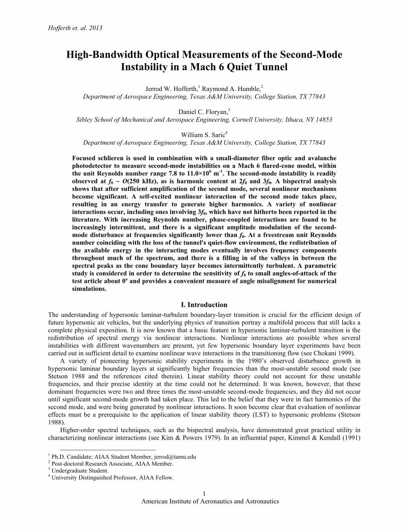
The model used in the present study is the Langley 93-10 flared cone studied by Lachowicz et. al.(1995, 1996) and Doggett et. al. (1997) in the M6QT’s former installation at NASA Langley, and later by Horvath et. al. (2002) in a conventional tunnel. Its geometry, depicted in figure 1, consists of a 5º half-angle right-circular conical profile for the first 0.25 m [10″] of axial distance, followed by a tangent flare of radius 2.36 m [93.071″] until the base of the cone at the 0.51 m [20″] axial station. The adverse pressure gradient imposed by the flare serves to destabilize the second-mode instability, promoting more substantial growth within the small test environment of the M6QT. The base diameter is 0.12 m. The model is of a thin-wall stainless steel construction with nominal wall thickness of 1.8 mm. The first 38 mm of length are removable to allow for selection of nose-tip radius; a sharp tip is used for the current study. For more on the cone model itself, see Lachowicz (1995) and Hofferth & Saric (2012a), which additionally describe the technique used for the determination of installed geometric alignment. For the analyses presented in §IV, the geometric alignment of the model was such that the measurement ray was 0.04º windward, with an out-of-plane misalignment ≈ 0.1º.

C. Focused schlieren apparatus

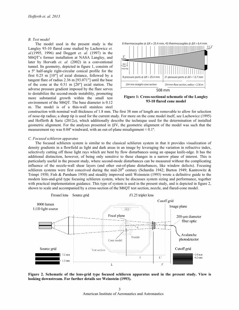
The focused schlieren system is similar to the classical schlieren system in that it provides visualization of density gradients in a flowfield as light and dark areas in an image by leveraging the variation in refractive index, selectively cutting off those light rays which are bent by flow disturbances using an opaque knife-edge. It has the additional distinction, however, of being only sensitive to these changes in a narrow plane of interest. This is particularly useful in the present study, where second-mode disturbances can be measured without the complicating influence of the nozzle-wall shear layers (and other out-of-plane disturbances, like window defects). Focusing schlieren systems were first conceived during the mid-20th century (Schardin 1942; Burton 1949; Kantrowitz & Trimpi 1950; Fish & Parnham 1950) and steadily improved until Weinstein (1993) wrote a definitive guide to the modern lens-and-grid type focusing schlieren system, where he discusses system sizing and performance, together with practical implementation guidance. This type of system is used in the present study, and is depicted in figure 2, shown to scale and accompanied by a cross-section of the M6QT test section, nozzle, and flared-cone model.

Figure 2. Schematic of the lens-grid type focused schlieren apparatus used in the present study. View is looking downstream. For further details see Weinstein (1993).

Figure 1: Cross-sectional schematic of the Langley 93-10 flared cone model



4

Classically, this type of system consists of an extended light source, two grids, and a lens. Boedeker (1959)

added a Fresnel lens after the light source in order to dramatically improve the image brightness. The source and cutoff grids are sets of alternating opaque and clear stripes, and are photographic negatives of each other. In this way, each pair of source and cutoff stripes function as the slit-source of light and knife edge cutoff of a conventional schlieren system. The system as a whole can be thought of as superposition of many conventional schlieren systems, with each clear stripe of the source grid and corresponding opaque stripe of the cutoff grid functioning as the light source and knife edge, respectively. This, along with a large lens aperture and non-collimated light path, lend the system its focusing ability.

For fixed locations of the source and cutoff grids relative to the lens (distances L and Lʹ, respectively), a focal plane location (distance l from the lens) can be chosen by selection of the image plane at distance lʹ from the lens. At the image plane, one may place a screen or camera and use a high-intensity pulsed light source for high-speed imaging. Alternatively, one may use the focused schlieren setup for high-bandwidth deflectometry, as is done for the present work. In this configuration, a constant light source is used, and a fiber optic is precisely placed in the image plane to correspond to a particular physical location in the focal plane. The fiber optic is then coupled to a high-bandwidth photodetector, enabling acquisition of time series of light intensity, and therefore, spectra of density fluctuations at a point in the image. Primary design goals were to obtain a focal depth less than 25 mm and a field-of-view of at least 25-50 mm, with maximum practical sensitivity and an overall system footprint suited to the spatial constraints of the M6QT laboratory. The integration of disturbances across the focal depth is not anticipated to pose a significant problem; over a range of supersonic and hypersonic Mach numbers, linear stability analysis predicts that the most unstable second mode disturbances are oriented normal to the freestream (k = 0, where k is the wavenumber). Therefore it is plausible that the harmonics are also two-dimensional disturbances (see e.g., Chokani 2005). A similar implementation of the technique has recently been made by VanDercreek (2010). Table 1 gives the chosen values for the key geometric parameters of the system, as well as two measures of the focal depth performance. Note w is the resolution limit of the image due to the grid geometry and image magnification.

Table 1. Key configuration parameters for the focused schlieren apparatus

Parameter Description Value A Lens aperture diameter 155 mm f Lens focal length 195 mm L Distance from lens to source grid 1444 mm Lʹ Distance from lens to cutoff grid 221 mm l Distance from lens to object plane 530 mm lʹ Distance from lens to image plane 308 mm

DS Depth of sharp focus (= 2lw/A) 0.97 mm DU Depth of “unsharp” focus (for 3 mm structure) (= 6l/A) 21 mm

In the present implementation, the extended light source is a

Bridgelux C8000LM high-power, 8000-lumen LED array driven with 3.0A current at 30.5V using a 95W Mean Well CEN-100 constant-current LED driver. The LED array is mounted to a large heat sink and surrounded by a shaped reflector to maximize light delivered to the system. The Fresnel lens is 317 mm in diameter with a 213 mm focal length. Traditionally, source and cutoff grids for focused schlieren systems are manufactured from photographic film, and one is exposed to be the negative of the other. However, for simplicity both the cutoff and source grids were printed on ordinary transparency film using a black-and-white laser printer from Adobe Photoshop source files. Special care was taken to maximize the opacity of the printed grid lines using the printer’s contrast and brightness controls, and to maximize the sharpness of the lines by matching the source files’ resolution to the printer’s native resolution.

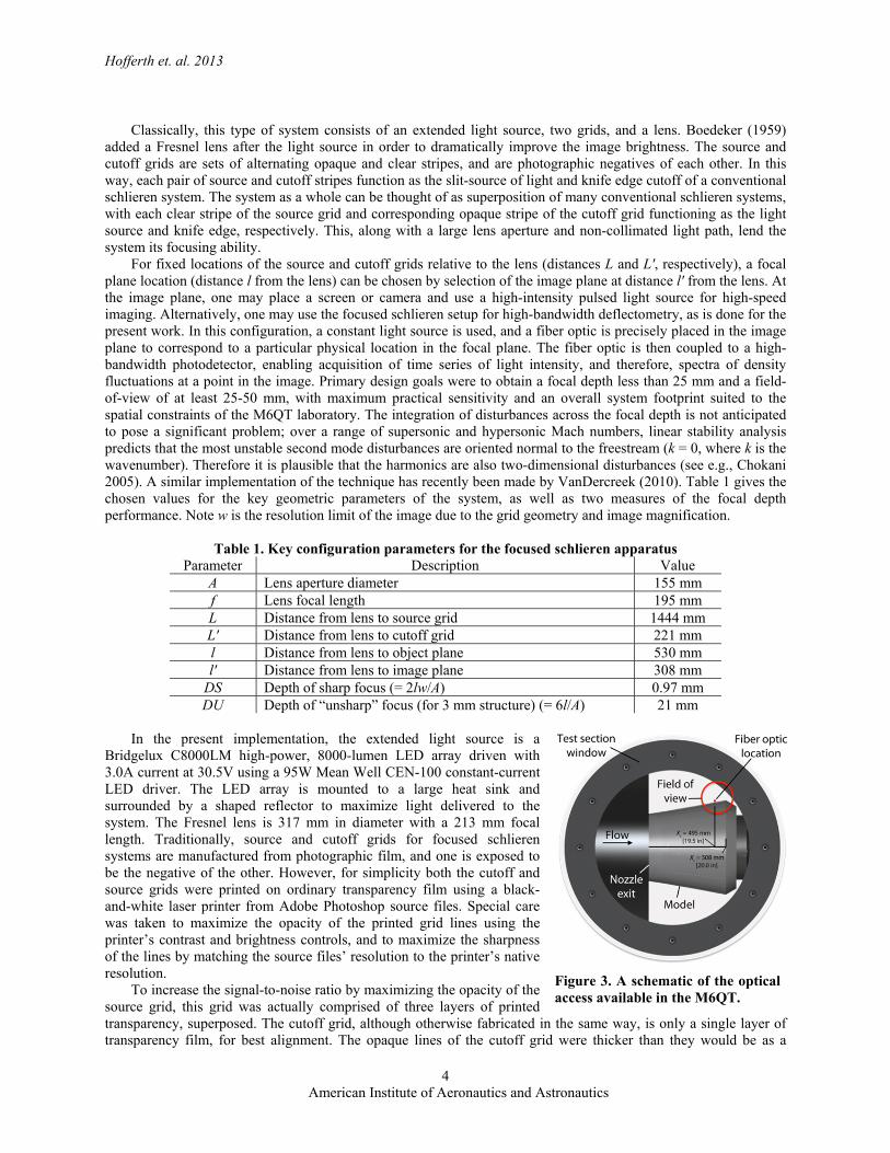
To increase the signal-to-noise ratio by maximizing the opacity of the source grid, this grid was actually comprised of three layers of printed transparency, superposed. The cutoff grid, although otherwise fabricated in the same way, is only a single layer of transparency film, for best alignment. The opaque lines of the cutoff grid were thicker than they would be as a

Figure 3. A schematic of the optical access available in the M6QT.



5

photographic negative of the source – this further improves signal-to-noise ratio by additionally cutting off unwanted residual light that bleeds through the opaque regions of the source grid. The lens is a three-element achromat 155 mm in diameter with a 195 mm focal length (f/1.25). The cutoff grid is mounted on a series of fine-resolution kinematics which allow for precision adjustment in the axial direction (for focus), tilt on two axes (for grid alignment), and vertical motion (for cutoff adjustment). Adjustment of the grids is performed by backlighting the cutoff grid from behind the image plane, and aligning its projection onto the source grid, ensuring proper magnification, focus, alignment, and cutoff. Figure 3 depicts the available optical access. High-quality dual surface optical flats mounted in the test section walls provided optical access through an aperture 190 mm in diameter, within which the nozzle exit and base of the cone are visible. Within this available optical pathway, the focused schlieren apparatus was positioned to select an effective field of view approximately 40 mm in diameter. For these experiments, the field-of-view was selected to be at the base of the upper surface of the cone. The fiber optic was positioned in the image plane such that its location in the cone boundary layer corresponded to an axial station Xc = 495 mm, where Xc = 0 is the location of the model’s sharp tip, and mean height of approximately 1.3 mm, previously observed to be the height of maximum instability amplitude for zero angle of attack. This height was adjusted as necessary for best measurement of leeward and windward conditions.

The fiber optic was coupled to a Thor Labs APD110A avalanche photodetector, which offered a voltage output with high sensitivity and a bandwidth of 50 MHz. The signal from the photodetector was fed to a Stanford Research Systems SR560 signal conditioner, amplified by a factor of 50, and filtered from 1 kHz to 1 MHz (–6 dB/decade). Both the raw and filtered/amplified signals were acquired during the run at a sampling rate of 2 MHz.

III. Bispectral Analysis A brief description of the bispectral analysis is provided to aid the interpretation of the results later on. Consider

a fixed location within the cone boundary layer where a finite record of fluctuating light intensity is extracted as the data series I'(n), n = 0, 1, …, T – 1, where T is the length of the time-series data. This time series can be divided into K segments, i = 0, 1, …, K – 1, each of length M. Let the ith segment of I(n) therefore be Ii(n), n = 0, 1, … , M – 1. The auto-bispectrum Bi(f1, f2) may be computed by

where f is a discrete frequency, * is the complex conjugate, and Xi(f) the ith discrete Fourier transform (DFT) for each segment. In practice, estimates from all K segments may be averaged to give

The bispectrum B(f1, f2) is a measure of the degree of nonlinear quadratic phase coupling between the signal

components at frequencies f1 and f2. Phase coupling occurs when the sum of the phase of the frequency components f1 and f2 is equivalent to the phase of the sum frequency (f1 + f2). If the triad of waves f1, f2 and (f1 + f2) are nonlinearly coupled, then f1 + f2 → (f1 + f2), where “→” denotes “generates by phase-coupled interaction” (see e.g., Chokani 1999). Furthermore, because the phase at the sum frequency, ϕ3, is simply the sum of the phases of the component frequencies, ϕ1 + ϕ2, then the biphase ϕ(f1, f2) at that frequency will be zero (or small), where the bicoherence is relatively high. Statistical averaging ensures that only meaningful nonlinear coupling between frequency components are retained. The bispectrum therefore discriminates between nonlinearly coupled waves and spontaneously excited waves, because spontaneously excited waves are generated independently of the other components, and thus have independent amplitudes and phases.

By virtue of the bispectrum symmetry,

which limits the total (useful) area to



6

where fN is the Nyquist frequency. There are a few difficulties, however, with the direct implementation of the bispectrum in this way. In particular is the fact that energetic spectral components with a moderate degree of phase coherence can dominate weaker spectral components with a higher degree of phase coherence. To resolve this and other issues, Kim & Powers (1979) suggest the use of the squared bispectrum, normalizing such that

where E is the expectation operator and b2(f1, f2) is known as the bicoherence. In what follows, the bicoherence is used, the advantage being that it is bounded by 0 and 1. A bicoherence of zero means completely independent waves, whereas a value of unity means completely coupled waves. It is worth noting that this is not the only way of normalizing the bispectrum (see Hinich & Wolinksy 2005 for further discussion), although it is one of the most popular and is sufficient for the present purposes. Due to the normalization, the symmetry relations for the bicoherence are different from the bispectrum. A symmetry has been lost, and we now have

IV. Results & Discussion A. Time series and power spectral density

To motivate the discussion, a time series segment (0.5 ms) is shown in figure 4 for each of the unit Reynolds numbers considered. Each case was obtained during the same run, and has been digitally high-pass filtered at 100 kHz to highlight the second-mode fluctuations. The fiber optic measurement location for all runs shown is Xc = 495 mm. Note that because the fiber optic height is fixed throughout the run, during which the boundary layer thickness and height of maximum fluctuation change with Re, amplitudes should not be directly compared. For each Re < 10.7×106 m-1, second-mode disturbances within the range 210–280 kHz are clearly observed. In each case, these instabilities appear in wave packets, with an amplitude envelope much lower in frequency. With increasing Re, the signal becomes increasingly irregular. By Re = 11.0×106 m-1, the signal appears fully turbulent. This behavior is expected, given the known loss of quiet flow in the M6QT freestream by approximately Re = 10.7×106 m-1; in this regard, the observed breakdown to turbulence is not a “natural” process in the conventional sense.

Figure 4. Segments of photodetector output time series for select unit Reynolds numbers during a single run. Voltages are high-passed at 100 kHz to highlight second-mode content between 210–280 kHz for Re < 10.7×106 m-1.



7

The global evolution of the spectral content with Re is depicted in figure 5(a). Spectra are computed for each 100 ms segment of the run using Welch’s method, averaging 50 windows with 75% overlap. At the lowest Reynolds number considered of 7.8×106 m-1, only the second-mode frequency f0 is essentially observed. Harmonics at 2f0 and then 3f0 become visible as Re increases, albeit at lower amplitudes. Note also that the frequencies of the instabilities increase gradually with increasing Re, due to the tuning of the second-mode instability to the boundary-layer thickness, δ. A turbulent state abruptly appears at approximately Re = 10.7×106 m-1.

Figure 5. (a) Spectrogram of photodetector power spectral density variation with unit Re during a single run. Each power spectrum is averaged over 100 ms of runtime. Re = 7.8 to 11.5×106 m-1, (b) power spectra at select Re taken from (a).

Figure 5(b) shows extracted power spectral densities for the selected unit Reynolds numbers shown, denoted by the dotted lines in Figure 5(a). The second-mode amplitude increases with increasing Re, and then by Re = 10.7×106 m-1, as the onset of turbulence is imminent, the well-defined peaks of the instability have fallen in amplitude. This is accompanied by valleys at frequencies between the harmonics, which become filled in with broadband fluctuation of turbulence. This suggests the possibility of an energy transfer between the modes. However, a major limitation of this representation is that phase information is lost in the Fourier analysis. To investigate the nonlinear interactions that give rise to the behavior observed, we turn to a bispectral analysis. B. Analysis of nonlinear interactions

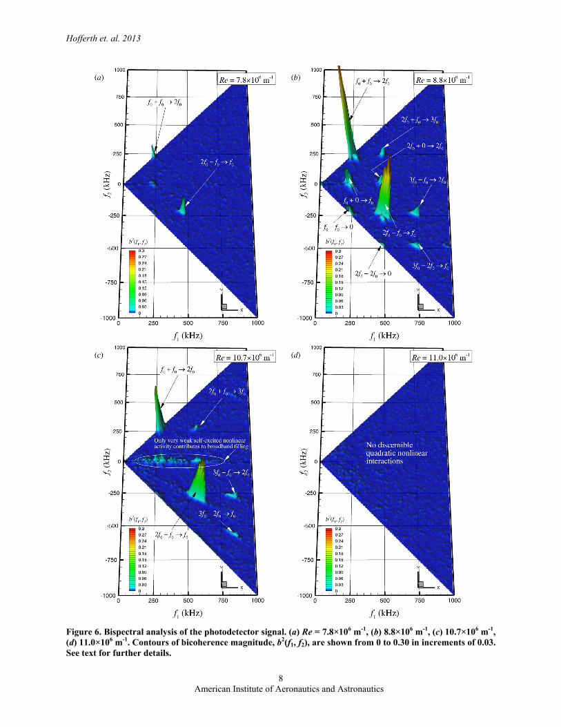
To examine the nonlinear phase-coupled quadratic interactions that give rise to the spectral components described above, a bispectral analysis is carried out. Figure 6 shows the magnitude of the normalized bispectrum magnitude, or bicoherence, b2(f1, f2). The bicoherence plots were computed from the unamplified, unfiltered photodetector signal using Hanning windows 256 points in length, with 50% overlap. For clarity, only results for sum interactions within the range (0, 0), (fN, fN), (fN, 0), and for difference interactions within the triad (0, 0), (fN, 0), (fN, –fN) are shown.

The results suggest the boundary layer contains a variety of quadratic phase-coupled interactions that appear to undergo a distinct evolution with unit Reynolds number. At Re = 7.8×106 m-1, the genesis of nonlinear interactions is just occurring, with weak sum interaction f0 + f0 → 2f0 and difference interaction 2f0 – f0 → f0. These interactions describe the very early stages of the second-mode’s nonlinear growth. Prior to this, the second mode undergoes a purely linear (exponential) growth; in this case no bicoherence peaks are expected to be present.

At Re = 8.8×106 m-1, a variety of nonlinear interactions emerge, indicating that the second mode undergoes significant nonlinear growth. Because the boundary layer is developing under natural forcing from freestream disturbances, the possibility exists that 2f0 (and 3f0 etc.) is an independent, spontaneously excited wave. This cannot be determined from the power spectral density alone because phase information is lost. However, from the bicoherence analysis it appears that 2f0 is the result of nonlinear wave propagation, because a phase relation exists between f0 and 2f0. This has been observed by Chokani (2005). Sum interactions exist involving the self-excited interaction f0 + f0 → 2f0, and 2f0 + f0 → 3f0. Thus, a small disturbance at f0 can reinforce itself substantially and transfer energy to the higher harmonics. Furthermore, because the phase at the sum frequency, ϕ3, is simply the sum of the phases of the component frequencies, ϕ1 + ϕ2, then the biphase ϕ(f1, f2) at the frequencies associated with significant bicoherence were zero (or at least small).



8

Figure 6. Bispectral analysis of the photodetector signal. (a) Re = 7.8×106 m-1, (b) 8.8×106 m-1, (c) 10.7×106 m-1, (d) 11.0×106 m-1. Contours of bicoherence magnitude, b2(f1, f2), are shown from 0 to 0.30 in increments of 0.03. See text for further details.



9

In addition, the difference interaction 2f0 – f0 → f0 is observed, consistent with the work of Chokani (2005) also under low-disturbance freestream conditions. This is accompanied by somewhat weaker interactions involving f0 + 0 → f0 and 2f0 + 0 → 2f0, whose concentration along the abscissa indicates that the valleys between the spectral peaks observed in the power spectrum are being filled. Barely perceptible interactions are also present at f0 – f0 → 0 and 2f0 – 2f0 → 0 (running along the lower diagonal line), which would suggest that the second mode and 2f0 lead to mean flow distortion. This is consistent with the fact that the boundary layer profiles still have the characteristics of a laminar boundary layer, in spite of the existence of these large disturbances (see Hofferth et al. 2012b). The elongated appearance of the bicoherence peaks suggests that the second mode is coupling with frequencies in its sidebands, serving to broaden the bands of the harmonics. (Notice how in the earlier stages of the (nonlinear) transition process at Re = 7.8×106 m-1, the bicoherence contours appear more circular and more localized in bifrequency space.) It is interesting to observe even higher-order harmonic interactions, involving 3f0 – f0 → 2f0 and 3f0 – 2f0 → f0, indicating that ultrahigh frequency components play a role in the nonlinear evolution of the disturbances. These are not generally accessible via hot-wire anemometry, and have not hitherto been reported in the literature.

As the unit Reynolds number increases to Re = 10.7×106 m-1, the nonlinear interactions outlined above decrease in bicoherence magnitude. Inspection of the time series reveals that phase-coupled nonlinear interactions take place increasingly intermittently (see also following subsection). The ensemble-averaged bicoherence magnitude therefore decreases. Interactions also occur involving f0 + δf → (f0 + δf) and f0 – δf → (f0 – δf), as well as 2f0 + δf → (2f0 + δf) and 2f0 – δf → (2f0 – δf), where δf spreads along much of the sideband extent. This has also not been previously observed (cf. Chokani 2005), at least not to the same extent. These interactions portray the valleys between the spectral peaks observed in the power spectrum being increasingly filled. However, the very small magnitude of these spectra-filling interactions (<0.05) supports the earlier observation that the broadband spectral content at this unit Re arises as a result of the onset of tunnel noise – an external forcing poorly phase-correlated with the instabilities on the cone. It is interesting to note, however, that despite the disappearance of several interactions at this stage, significant sum and difference interactions involving f0 + f0 → 2f0 and 2f0 – f0 → f0, respectively, still remain.

Finally, at Re = 11.0×106 m-1, significant nonlinear phase-coupled interactions are no longer detected. This could be because any nonlinear interaction present are no longer quadratic, or because the remaining fluctuations are now random. The results collectively suggest that high-frequency nonlinear disturbances are not confined to a small region associated with the breakdown to turbulence, but are present for a significant portion of the laminar boundary-layer development (see Stetson 1998), and can be present when only the second-mode frequency exists in the power spectral density.

Since the main features of the bicoherence distributions portraying the nonlinear coupling mechanisms do not change significantly with unit Reynolds number (as verified by considering other intermediate Reynolds numbers not shown here for brevity), this suggests that the spectral valley filling, and the harmonic generation process, are likely governed by the same generic nonlinear interaction mechanisms. Similar conclusions have been drawn by others who have considered the nonlinear dynamics of transitioning flows (e.g., Miksad et al. 1983; Ritz et al. 1988). The present nonlinear mechanisms appear to be associated with a redistribution of the available energy in the interacting modes, characterized by the higher-order harmonics gaining enough energy to couple with the second mode to generate even higher harmonics, eventually involving frequency components throughout the whole spectrum. The increased spectral bandwidth of the present results compared to previous studies shows that these nonlinear interactions involve even higher harmonics of the second-mode disturbance than previously observed.

C. Second-mode intermittency and amplitude modulation

It is clear from the above, that perfect phase-coupling between all of the interactions is not present at all times. To investigate this intermittency, the temporal evolution of the spectral content may be conveniently described by the short-time FFT (256 samples per Hamming window, 50% overlap). These spectrograms are shown in figure 7(a–c) for Re = 10.4, 10.7, and 11.0×106 m-1, respectively. From these results, it is clear that the appearance of the second-mode instability, its harmonics, and consequently the spectral redistribution of energy between them become increasingly intermittent with increasing Re. It is believed that this intermittency is not representative of any natural process of breakdown of the flared cone boundary layer, but instead directly results from the rapid onset of heavy intermittency of test environment flow quality as the unit Reynolds number increases. That is, the location of the onset of turbulence is likely intermittently alternating between that for quiet flow (Xc > 430 mm) and that for noisy flow (Xc ≈ 280 mm). For further details on the characterization of the freestream flow, the reader is referred to Hofferth et al. (2010).



10

Figure 7. Short-time FFT spectrograms of the photodetector signal at three unit Reynolds numbers. (a) Re = 10.4×106 m-1, (b) Re = 10.7×106 m-1, (c) Re = 11.0×106 m-1. The freestream condition in (b) coincides with the loss of quiet flow in the freestream test environment.

The above intermittency also manifests itself as, or is at least associated with, an amplitude modulation of the

second-mode disturbance. This amplitude modulation may be characterized in more detail by first determining the envelope of the carrier signal. This may be accomplished, among other ways, by creating a complex analytic signal using the Hilbert transform. The real part of the analytic signal is the original signal, and the imaginary part is the Hilbert transform. The signal is band-pass filtered at the carrier frequency f0 to avoid the demodulation of several signals (using a bandwidth Δf = 20 kHz, centered on f0 for each Re), and to focus on the low-frequency amplitude modulations. Figure 8(a) shows a segment of the Hilbert amplitude, or signal envelope. The second mode disturbance is clearly modulated by amplitudes of various frequencies, which are appreciably lower than f0 itself.

Premultiplying the usual power spectral density of the signal’s envelope by the wavenumber k provides a different interpretation to the results. The usual reason for premultiplying by the wavenumber is to create a logarithmic plot in which equal areas under the graph correspond to equal energies. This stems from the equality: ∫ E(k) dk = ∫ kE(k) dlogk; hence, a plot of kE(k) against logk is variance preserving. This type of representation has been an indispensible tool in turbulence research for investigating large-scale coherent motions, which are typically associated with wavelengths much larger than the boundary-layer thickness (see e.g., Kim & Adrian 1999). In the present study, the abscissa is expressed for convenience in terms of a wavelength λ = 2π/k, normalized by a characteristic length associated with the second mode, in this case 2δ, where δ (= 1.5 mm) is the local boundary layer thickness (assumed constant in the present study although this does not affect the conclusions drawn). The premultiplied spectra are shown in figure 8(b), where all spectra are normalized to unit area, to emphasize their frequency (wavelength) content. The premultiplied spectra were computed from the unamplified, unfiltered signal using a 4096-point FFT with 75% overlap, in order to better resolve the larger wavelengths. The results confirm energetic wavelengths appreciably larger than the one associated with the second mode, implying that the second mode disturbance amplitude is modulated over significantly lower frequencies than f0. This is consistent with the observations of Chokani (2005), who used complex demodulation to determine his amplitude and phase modulates. A broad range of most-energetic wavelengths are found to occur at around 10λ/2δ, which corresponds to O(20) kHz. Recognizing a significant variation in amplitude modulation, a typical wave packet therefore, on average, contains O(10) second mode oscillations. As the Re increases, it appears as though energy shifts, within this admittedly narrow Re range, from the smaller wavelengths to the larger ones. It is speculated that these modulations are associated with the intermittent nature of the disturbances radiating from the transitioning nozzle-wall boundary layer, and that as the Re increases, the attendant increase in intermittency exacerbates the amplitude modulation, thereby reducing the energetic wavelengths of the signal’s envelope. However, further work needs to be conducted before any substantial claims can be made.



11

Figure 8. Second-mode amplitude modulation analysis. (a) Selected portion of the bandpass signal (blue) with signal envelope (red) for Re = 10.4 × 106 m-1, (b) premultiplied power spectrum kδE(k) of the envelope for several Re.

V. Conclusions & Future Work A focusing schlieren system in combination with an avalanche photodetector and fiber optic has been

implemented to study second-mode instabilities on a flared-cone model. The diagnostic technique is well-suited to the experiment, where the two-dimensionality of the instability combines with the shallow focal depth of the technique to produce spectra of the instability with high sensitivity and high signal-to-noise ratio. A bispectral analysis shows that after sufficient amplification of the second mode, several nonlinear mechanisms become significant. A self-excited nonlinear interaction of the second mode takes place, resulting in an energy transfer to generate a harmonic via phase-coupled quadratic interaction, as observed by others using hot-wire anemometry. Subsequent nonlinear interactions of the second mode disturbance and this harmonic lead to the generation of a higher harmonic. With increasing Reynolds number, phase-coupled interactions are found to be increasingly intermittent, and there is a significant amplitude modulation of the second-mode disturbance at significantly lower frequencies than f0. At a freestream unit Reynolds number coinciding with the loss of the tunnel's quiet-flow environment, the redistribution of the available energy in the interacting modes eventually involves frequency components throughout much of the spectrum, and there is a filling in of the valleys in between the spectral peaks as the cone boundary layer becomes intermittently turbulent.

Several issues remain, however, including how generic the aspects of the nonlinear interactions really are, as presently characterized at a single location, and by varying the Reynolds number via the total pressure and not cone measurement location. The relatively low-frequency amplitude modulation of the second-mode instability warrants further study, as well as the role of the intermittent freestream disturbances that radiate from the nozzle-wall boundary layer. Also, only frequency-matching was considered in the present study. Future efforts should consider multiple measurement locations, including wavenumber matching from wavenumber-frequency power spectra. Artificial excitation in the freestream would be very instructive in order to further investigate the modulation influences of the freestream on the second-mode disturbance development.



12

Appendix A: Cone Misalignment and Second-Mode Sensitivity Assessment Recent comparisons between numerical simulations utilizing LPSE and experiments using both constant-

temperature hot-wire anemometry (CTA) and FSD have revealed a discrepancy in the frequency of the second-mode instability. The computed most-amplified frequencies for the second mode at zero angle of attack were over 40 kHz lower than observed in the hot-wire experiments of Hofferth et. al. 2012b (234 kHz versus 280 kHz, respectively). Figure A1 provides a comparison of power spectra from both focused schlieren and CTA for Xc = 495 mm and Re = 10×106 m-1. Computations of integrated growth from LPSE are shown as well.

Possible explanations for this discrepancy are numerous, including model misalignment along the measurement ray, inadequate wall-temperature conditions in the simulation, or possibly an under-damped hot-wire transfer function artificially amplifying higher frequencies. Believed to be dominant among these was the effect of slight model misalignment, although the sensitivity to this was not well understood.

Figure A1. Significant discrepancy between second-mode most-amplified frequencies, f0, computed via LPSE and observed in power spectral density from CTA and FSD methods. CTA power spectra and LPSE N-factor data from Hofferth et. al. (2012b).

In order to experimentally determine the sensitivity of f0 to small angles of incidence, the model incidence was set for each in a series of 8 runs to a different pitch angle between -1º and +1º, taking care to minimize the yaw angle, which was typically kept under 0.2º. Geometric alignment for each run was quantified using the confocal laser scan method described in Hofferth & Saric (2012a). The robust, non-intrusive nature of the focused schlieren system made it an excellent candidate for a tedious campaign such as this, which required a substantial amount of work inside the test section between runs, carefully manipulating the model alignment and then setting up and conducting a new scan with the confocal laser each time.

For each run, a typical Reynolds number sweep was conducted. From the Re = 10×106 m-1 condition, an averaged spectra was computed, from which the fundamental frequency, f0, was programmatically identified. Figure A2 shows the values of f0 identified for each of the model incidences at Re = 10×106 m-1 as the empty circular markers. Also plotted here are the curious hot-wire data from Hofferth et. al. (2012b) and three LPSE-computed results from the work of Perez et. al. (2012). The slope of the best-fit line through the deflectometry data is –84 kHz per degree (or 8.4 kHz per a mere 0.1º misalignment). Note in particular the red error bars of Figure A2. These serve to provide a notional prediction of the effect of small out-of-plane misalignment (< 0.3º for each point) as measured by the laser scan technique. When the measurement ray is under a nominally windward condition, any out-of-plane misalignment serves to thicken the boundary layer and reduce f0. When the measurement ray is under a nominally leeward condition, any out-of-plane misalignment thins the boundary layer, and increases f0. Because the effect of this is one-sided, the 8.4 kHz/0.1º best-fit slope is necessarily over-predicted for purely in-plane misalignments. The three data points available from the LPSE computations (blue squares) show a sensitivity of 6.5 kHz per 0.1º – indeed, a shallower slope. Regardless, this direct knowledge of a practical sensitivity to pitch misalignment within practical limits of out-of-plane residual misalignment is valuable for motivating an increased level of caution when installing and aligning the model for second-mode study at 0º nominal incidence.



13

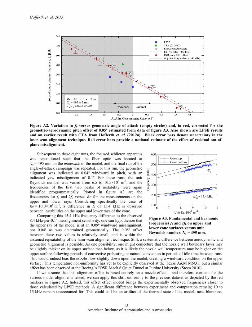
Figure A2. Variation in f0 versus geometric angle of attack (empty circles) and, in red, corrected for the geometric-aerodynamic pitch offset of 0.05º estimated from data of figure A3. Also shown are LPSE results and an earlier result with CTA from Hofferth et. al. (2012b). Black error bars denote uncertainty in the laser-scan alignment technique. Red error bars provide a notional estimate of the effect of residual out-of-plane misalignment.

Subsequent to these eight runs, the focused schlieren apparatus

was repositioned such that the fiber optic was located at Xc = 495 mm on the underside of the model, and the final run of the angle-of-attack campaign was repeated. For this run, the geometric alignment was indicated as 0.04º windward in pitch, with an indicated yaw misalignment of 0.1º. For these runs, the unit Reynolds number was varied from 6.5 to 10.5×106 m-1, and the frequencies of the first two peaks of instability were again identified programmatically. Plotted in figure A3 are the frequencies for f0 and 2f0 versus Re for the measurements on the upper and lower rays. Considering specifically the case of Re = 10.0×106 m-1, a difference in f0 of 15.4 kHz is observed between instabilities on the upper and lower rays of the cone.

Comparing this 15.4 kHz frequency difference to the observed 8.4 kHz-per-0.1º misalignment sensitivity, one can hypothesize that the upper ray of the model is at an 0.09º windward misalignment, not 0.04º as was determined geometrically. The 0.05º offset between these two values is relatively small, and is within the assumed repeatability of the laser-scan alignment technique. Still, a systematic difference between aerodynamic and geometric alignment is possible. As one possibility, one might conjecture that the nozzle wall boundary layer may be slightly thicker on its upper surface than below, as it is likely the nozzle wall temperature may be higher on the upper surface following periods of convective preheating or natural convection in periods of idle time between runs. This would indeed bias the nozzle flow slightly down upon the model, creating a windward condition on the upper surface. This temperature non-uniformity has yet to be explicitly observed at the Texas A&M M6QT, but a similar effect has been observed at the Boeing/AFOSR Mach 6 Quiet Tunnel at Purdue University (Steen 2010).

If we assume that this alignment offset is based entirely on a nozzle effect – and therefore constant for the various model alignments tested, we can apply this shift uniformly to the previous dataset as depicted by the red markers in Figure A2. Indeed, this offset effect indeed brings the experimentally observed frequencies closer to those calculated by LPSE methods. A significant difference between experiment and computation remain; 10 to 15 kHz remain unaccounted for. This could still be an artifact of the thermal state of the model, nose bluntness,

Figure A3. Fundamental and harmonic frequencies f0 and 2f0 on upper and lower cone surfaces versus unit Reynolds number. Xc = 495 mm.



14

misalignment or flow angularity about the yaw axis, or other effects. However, now that the sensitivities are known, it is valuable to be able to confidently state that the remaining difference between experiment and computation amounts to perhaps only 0.2º in model misalignment. Although this number is small and may be regarded as within practical limits of error, the effect on f0 is large, motivating even closer collaboration between experiment and computation, as well as improved model alignment adjustment & characterization techniques for future work.

Acknowledgments The authors would like to thank Nick Parziale for his assistance with the initial configuration of the focused

schlieren apparatus. Support from the AFOSR/NASA National Center for Hypersonic Research in Laminar-Turbulent Transition through Grant FA9550-09-1-0341 is also gratefully acknowledged.

References Boedeker, L. R. 1959. Analysis and Construction of a Sharp Focussing Schlieren System. M.S. Thesis. Massachusetts Institute of

Technology. Blanchard, A. E., Lachowicz, J. T. & Wilkinson, S. P. 1997 NASA Langley Mach 6 Quiet Wind-Tunnel Performance. AIAA J.

35(1):23–28. Burton, R. A. 1949. A Modified Schlieren Apparatus For Large Areas Of Field. JOSA 39(11):907–908. Chen F-J., Wilkinson S. P. & Beckwith, I. E. 1993. Görtler Instability and Hypersonic Quiet Nozzle Design. J. Spacecraft and

Rockets 30(2):170–175. Chokani, N. D. 1999. Nonlinear Spectral Dynamics of Hypersonic Boundary Layer Flow. Phys. Fluids 11(12):3846–3851. Chokani, N. D. 2005. Nonlinear Evolution of Mack Modes. Phys. Fluids 17(1):014102. Doggett, G. P., Chokani, N. D. & Wilkinson, S. P. 1997. Hypersonic Boundary-Layer Stability Experiments on a Flared-Cone

Model at Angle of Attack in a Quiet Wind Tunnel. AIAA Paper 1997-0557. Fish, R. W. & Parnham, K. 1950. Focussing Schlieren Systems. Report CP-54, British Aeronautical Research Council. Hinich, M. J. & Wolinsky, M. 2005. Normalizing Bispectra. Journal of Statistical Planning and Inference 130, 405–411. Hofferth, J. W., Bowersox R. D. W. & Saric W. S. 2010. The Mach 6 Quiet Tunnel at Texas A&M: Quiet Flow Performance.

AIAA Paper 2010-4794. Hofferth, J. W. & Saric, W. S. 2012a. Boundary-Layer Transition on a Flared Cone in the Texas A&M Mach 6 Quiet Tunnel.

AIAA Paper 2012-0923. Hofferth, J. W., Saric, W. S., Kuehl, J. J., Perez, E., Kocian, T. S. & Reed, H.L. 2012b. Boundary-Layer Instability and

Transition on a Flared Cone in a Mach 6 Quiet Wind Tunnel. RTO/AVT Specialists Meeting on Hypersonic Laminar-Turbulent Transition: AVT-200/RSM-030. San Diego, CA, USA. Paper No. 10.

Horvath, T. J., Berry, S. A., Hollis, B. R., Chang, C. L. & Singer, B. A. 2002. Boundary-Layer Transition on Slender Cones in Conventional and Low Disturbance Mach 6 Wind Tunnels. AIAA Paper 2002-2743.

Kantrowitz, A. & Trimpi, R. L. 1950. A Sharp-Focusing Schlieren System. J. Aero. Sci. 17:311-319. Kim, K. C. & Adrian, R. J. 1999. Very Large-Scale Motion in the Outer Layer. Phys. Fluids 11:417–422. Kim, Y. C. & Powers, E. J. 1979. Digital Bispectral Analysis and its Applications to Nonlinear Wave Interactions. IEEE Trans.

Plasma Science 7, 120–131. Kimmel, R. L. & Kendall, J. M. 1991. Nonlinear Disturbances in a Hypersonic Boundary Layer. AIAA Paper No. 1991-0320. Perez, E., Kocian, T. S., Kuehl, J. J. & Reed, H. L. 2012. Stability of Hypersonic Compression Cones. AIAA Paper 2012-2962. Lachowicz, J. T., Chokani, N. D. & Wilkinson, S. P. 1996. Boundary Layer Stability Measurements in a Hypersonic Quiet

Tunnel. AIAA J. 34(12):2496–2500. Lachowicz, J. T. Hypersonic Boundary Layer Stability Experiments in a Quiet Wind Tunnel with Bluntness Effects. Ph.D.

Dissertation, Mechanical and Aerospace Engineering Dept., North Carolina State Univ., Raleigh, NC. November 1995. Laurence, S. J., Wagner, A. & Hannemann, K. 2012. Time-Resolved Visualization of Instability Waves in a Hypersonic

Boundary Layer. AIAA J. 50:243–246. Miksad, R. W., Jones, F. L. & Powers, E. J. 1983. Measurements of Nonlinear Interactions during Natural Transition of a

Symmetric Wake. Phys. Fluids 26:1402–1409. Ritz, Ch. P., Powers, E. J., Miksad, R.W. & Solis, R. S. 1988. Nonlinear spectral dynamics of a transitioning flow. Phys. Fluids

31:3577–3588. Schardin, H. 1942. Die Schlierenverfahren une ihre Anwendungen. Ergebnisse der Exakten Naturwissenschaften, 20:303–439.

English translation available as NASA TT F-12731, April 1970 (N70-25586). Steen, L. E. 2010. Characterization and Development of Nozzles for a Hypersonic Quiet Wind Tunnel. M.S. Thesis. Purdue

University, West Lafayette, Indiana. Stetson, K. F. 1988. On Nonlinear Aspects of Hypersonic Boundary-Layer Stability. AIAA J. 26(7):883–885. VanDercreek, C. P. 2010. Hypersonic Application of Focused Schlieren and Deflectometry. M.S. Thesis. University of Maryland,

College Park. Weinstein, L. M. 1993. Large-Field High-Brightness Focusing Schlieren System. AIAA J. 31(7):1250–1255.

Documents

High-Bandwidth Optical Measurements of the Second-Mode