High Dimensional Expanders

Thesis submitted for the degree of “Doctor of Philosophy”

By

Ori Parzanchevski

Submitted to the Senate of the Hebrew University of Jerusalem

September 2013

This work was carried out under the supervision of:

Professor Alexander Lubotzky

2

Abstract

This work studies the relation between spectral and combinatorial expansion in simpli-cial complexes. More precisely, we study the spectrum of the simplicial Hodge Laplaciandefined by Eckmann, generalizing well known theorems from graph theory: the Cheegerinequalities concerning a graph’s isoperimetric constant; the “Expander Mixing Lemma”;properties of random walks and return probabilities; the theorems of Alon-Boppana andof Kesten regarding infinite trees; the study of random complexes, and of “Ramanujancomplexes”, and Gromov’s geometric overlap property.

3

Contents

1 Introduction 51.1 Isoperimetric constant . . . . . . . . . . . . . . . . . . . . . . . . . . . . . . . . . . . . . 61.2 Expander Mixing Lemmas . . . . . . . . . . . . . . . . . . . . . . . . . . . . . . . . . . . 71.3 Examples and applications . . . . . . . . . . . . . . . . . . . . . . . . . . . . . . . . . . . 91.4 High dimensional random walk . . . . . . . . . . . . . . . . . . . . . . . . . . . . . . . . 101.5 Infinite complexes . . . . . . . . . . . . . . . . . . . . . . . . . . . . . . . . . . . . . . . 131.6 Isospectrality . . . . . . . . . . . . . . . . . . . . . . . . . . . . . . . . . . . . . . . . . . 14

2 Preliminaries 162.1 Simplicial Hodge Laplacians . . . . . . . . . . . . . . . . . . . . . . . . . . . . . . . . . . 182.2 The spectrum of complexes . . . . . . . . . . . . . . . . . . . . . . . . . . . . . . . . . . 192.3 Complexes with a complete skeleton . . . . . . . . . . . . . . . . . . . . . . . . . . . . . 20

3 Isoperimetric constant 243.1 A Cheeger-type inequality . . . . . . . . . . . . . . . . . . . . . . . . . . . . . . . . . . . 243.2 Towards a lower Cheeger inequality . . . . . . . . . . . . . . . . . . . . . . . . . . . . . . 26

4 Mixing and pseudo-randomness 304.1 The complete skeleton case . . . . . . . . . . . . . . . . . . . . . . . . . . . . . . . . . . 304.2 The general case . . . . . . . . . . . . . . . . . . . . . . . . . . . . . . . . . . . . . . . . 32

5 Examples and Applications 375.1 Gromov’s geometric overlap . . . . . . . . . . . . . . . . . . . . . . . . . . . . . . . . . . 375.2 Chromatic bounds . . . . . . . . . . . . . . . . . . . . . . . . . . . . . . . . . . . . . . . 395.3 Ideal expanders . . . . . . . . . . . . . . . . . . . . . . . . . . . . . . . . . . . . . . . . . 405.4 Linial-Meshulam complexes . . . . . . . . . . . . . . . . . . . . . . . . . . . . . . . . . . 405.5 Ramanujan triangle complexes . . . . . . . . . . . . . . . . . . . . . . . . . . . . . . . . 42

6 High dimensional random walk 506.1 The (d− 1)-walk and expectation process . . . . . . . . . . . . . . . . . . . . . . . . . . 506.2 Normalized Laplacians . . . . . . . . . . . . . . . . . . . . . . . . . . . . . . . . . . . . . 516.3 Walk and spectrum . . . . . . . . . . . . . . . . . . . . . . . . . . . . . . . . . . . . . . . 55

7 Infinite complexes 597.1 Infinite graphs . . . . . . . . . . . . . . . . . . . . . . . . . . . . . . . . . . . . . . . . . 597.2 Infinite complexes of general dimension . . . . . . . . . . . . . . . . . . . . . . . . . . . 597.3 Example - arboreal complexes . . . . . . . . . . . . . . . . . . . . . . . . . . . . . . . . . 607.4 Continuity of the spectral measure . . . . . . . . . . . . . . . . . . . . . . . . . . . . . . 657.5 Alon-Boppana type theorems . . . . . . . . . . . . . . . . . . . . . . . . . . . . . . . . . 677.6 Analysis of balls in T 2

2 . . . . . . . . . . . . . . . . . . . . . . . . . . . . . . . . . . . . . 707.7 Spectral radius and random walk . . . . . . . . . . . . . . . . . . . . . . . . . . . . . . . 747.8 Amenability, transience and recurrence . . . . . . . . . . . . . . . . . . . . . . . . . . . . 75

8 Isospectrality 788.1 G-sets . . . . . . . . . . . . . . . . . . . . . . . . . . . . . . . . . . . . . . . . . . . . . . 788.2 Action and spectrum . . . . . . . . . . . . . . . . . . . . . . . . . . . . . . . . . . . . . . 818.3 Construction of unbalanced pairs . . . . . . . . . . . . . . . . . . . . . . . . . . . . . . . 848.4 Computation . . . . . . . . . . . . . . . . . . . . . . . . . . . . . . . . . . . . . . . . . . 90

9 Generalizations and open questions 92

4

1 Introduction

Most of my PhD research was devoted to the ongoing quest of understanding “high-dimensional ex-panders”. Expanders are sparse graphs which are highly connected. This is manifested in their geome-try (isoperimetric constant), combinatorics (pseudo-randomness), and dynamics (behavior of randomwalks), but it turns out that the notion of spectral expansion - boundedness of the Laplace spectrumof the graph - is often the most useful for mathematical analysis. In my study I sought to generalizethese notions of expansion to simplicial complexes of higher dimension, and to connect them to thespectrum of the high-dimensional Laplacian defined in the 1940’s by Eckmann. My study, severalparts of which were conducted in collaboration with other PhD students in our department, concernsseveral notions of expansion and related questions:

• Isoperimetric constant: this is a generalization of the Cheeger constant of graphs. It was studied,in joint work with Ron Rosenthal and Ran Tessler in [PRT14], and the results appear here in §3.

• pseudo-randomness (mixing): this is a natural notion of combinatorial expansion, which is closein spirit to the isoperimetric constant. This study is described in [PRT14, Par13a], and herein §4.

• Dynamical expansion: together with Ron Rosenthal I have defined and studied a stochasticprocess which generalizes random walks on graphs, and gives a notion of dynamic expansionwhich relates to the homology of a complex. This is described in [PR12, §2] and here in §6.

• Geometric overlap: this is a notion of expansion which is due to Gromov. Its relation to high-dimensional spectral expansion is explained in §5.1.

• Random complexes: random graphs are excellent expanders. Together with Ron Rosenthal Ihave studied the expansion properties of Random Linial-Meshulam complexes, and the resultsare described in [PRT14, §4.5] and here in §5.4

• Ramanujan complexes: these complexes are high-dimensional analogues of the Ramanujan graphsconstructed in [LPS88]. Together with Konstantin Golubev I have studied the spectral andcombinatorial properties of triangle Ramanujan complexes. Some of our results appear in §5.5.

• Asymptotic questions: in [PR12, §3] Ron Rosenthal and I have studied the spectrum of infinitecomplexes and questions concerning sequences of complexes, generalizing results of Kesten andof Alon-Boppana. This is described in §7.

Apart from spectral expansion, I have studied isospectrality : the challenge of constructing geometricobjects (graphs, complexes, manifolds and orbifolds) which have the same Laplace spectrum. Theresults appear in §8, which is based on [Par13b]. Another research I was involved in during myPhD studies is that of words in free groups. The results are not described here, and appear in[PS13, PP14a, PP14b]. The rest of this section gives a summary of the work and its main results.

5

1.1 Isoperimetric constant

The Cheeger constant of a finite graph G = (V,E) on n vertices is usually taken to be

ϕ (G) = minA⊆V

0<|A|≤n2

|E (A, V \A)||A|

where E (A,B) is the set of edges with one vertex in A and the other in B. In this work, however, weuse the following version:

h (G) = min0<|A|<n

n |E (A, V \A)||A| |V \A|

. (1.1)

Since ϕ (G) ≤ h (G) ≤ 2ϕ (G), defining expanders by ϕ or by h is equivalent. The spectral gap of G,denoted λ (G), is the second smallest eigenvalue of the Laplacian ∆+ : RV → RV , which is defined by

(∆+f

)(v) = deg (v) f (v)−

∑w∼v

f (w) . (1.2)

The discrete Cheeger inequalities [Tan84, Dod84, AM85, Alo86] relate the Cheeger constant and thespectral gap:

h2 (G)

8k≤ λ (G) ≤ h (G) , (1.3)

where k is the maximal degree of a vertex in G.(†) In particular, the bound λ ≤ h shows that spectralexpanders are combinatorial expanders. This proved to be of immense importance since the spectralgap is approachable by many mathematical tools (coming from linear algebra, spectral methods, rep-resentation theory and even number theory - see [HLW06, Lub10, Lub12a] and the references within).In contrast, the Cheeger constant is usually hard to analyze directly, and even to compute it for agiven graph is NP-hard [BKV+81, MS90].

Moving on to higher dimension, let X be an (abstract) simplicial complex with vertex set V . Thismeans that X is a collection of subsets of V , called cells (and also simplexes, faces, or hyperedges),which is closed under taking subsets, i.e., if σ ∈ X and τ ⊆ σ, then τ ∈ X. The dimension of a cell σis dimσ = |σ| − 1, and Xj denotes the set of cells of dimension j. The dimension of X is the maximaldimension of a cell in it. The degree of a j-cell (a cell of dimension j) is the number of (j + 1)-cellswhich contain it. Throughout this work we denote by d the dimension of the complex at hand, andby n the number of vertices in it (which will be finite except for Section 7). We shall occasionally addthe assumption that the complex has a complete skeleton, by which we mean that every possible j-cellwith j < d belongs to X.

We define the following generalization of the Cheeger constant:

Definition 1.1. For a finite d-complex X with n vertices V ,

h (X) = minV=

∐di=0 Ai

n · |F (A0, A1, . . . , Ad)||A0| · |A1| · . . . · |Ad|

,

(†) For ϕ they are given by ϕ2(G)2k

≤ λ (G) ≤ 2ϕ (G) .

6

where the minimum is taken over all partitions of V into nonempty sets A0, . . . , Ad, and F (A0, . . . , Ad)

denotes the set of d-dimensional cells with one vertex in each Ai.

For d = 1, this coincides with the Cheeger constant of a graph (1.1). To formulate an analogue ofthe Cheeger inequalities, we need a high-dimensional analogue of the spectral gap. Such an analogueis provided by the work of Eckmann on discrete Hodge theory [Eck44]. In order to give the definitionwe shall need more terminology, and we defer this to §2.2(†). The basic idea, however, is the same asfor graphs, namely, the spectral gap λ (X) is the smallest nontrivial eigenvalue of a suitable Laplaceoperator. The following theorem, whose proof appears in §3.1, generalizes the upper Cheeger inequalityto higher dimensions:

Theorem 1.2 (Cheeger Inequality, [PRT14]). For a finite complex X with a complete skeleton,λ (X) ≤ h (X).

Remarks. (1) If the skeleton of X is not complete, then h (X) = 0, since there exist somev0, . . . , vd−1 /∈ Xd−1, and then F (v0 , v1 , . . . , vd−1 , V \ v0, . . . , vd−1) = 0. This sug-gests that a different definition of h is called for. We give such a definition in §5.5 (see (5.10)),and a corresponding Cheeger inequality is proved in Theorem 5.9. A different generalization ofh appears in the open questions section §9.

(2) The existence of a lower Cheeger inequality is still an open question, and some progress in thisdirection is described in §3.2.

In [LM06] Linial and Meshulam introduced the following model for random simplicial complexes:for a given p = p (n) ∈ (0, 1), X (d, n, p) is a d-dimensional simplicial complex on n vertices, witha complete skeleton, and with every d-cell being included independently with probability p. UsingTheorem 1.2 we show in §5.4 the following:

Proposition 1.3. Let X = X(d, n, C logn

n

).

(1) For large enough C, a.a.s. h (X) ≥(C −O

(√C))

log n.

(2) For C < 1, a.a.s. h (X) = 0.

The proof appears as part of Corollary 5.7.

1.2 Expander Mixing Lemmas

The Cheeger inequalities (1.1) bound the expansion along the partitions of a graph, in terms of itsspectral gap. Nevertheless, a large spectral gap does not suffice to control the number of edges betweenany two sets of vertices. For example, the bipartite Ramanujan graphs constructed in [LPS88, MSS13]are regular graphs with very large spectral gaps, which are bipartite. This means that they containdisjoint sets A,B ⊆ V of size n

4 , with E (A,B) = ∅. The Expander Mixing Lemma [FP87, AC88,BMS93] (see also [HLW06]) remedies this inconvenience, using not only the spectral gap but also themaximal eigenvalue of the Laplacian:

(†) The spectral gap appears in Definition 2.2, and is given alternative characterizations in Proposition 2.4.

7

Theorem (Expander Mixing Lemma, [FP87, AC88, BMS93]). Let G = (V,E) be a graph on n vertices.If the nontrivial spectrum of its Laplacian is contained within [k − ρ, k + ρ], then for any two sets ofvertices A,B one has ∣∣∣∣|E (A,B)| − k |A| |B|

n

∣∣∣∣ ≤ ρ ·√|A| |B|. (1.4)

If k is the average degree of a vertex in G, then k|A||B|n is about the expected size of |E (A,B)| (the

exact value is kn−1 |A| |B|). Thus, the Lemma means that a concentrated spectrum indicates a pseudo-

random behavior. The deviation of |E (A,B)| from its expected value p |A| |B|, where p = kn ≈ |E|/(n2)

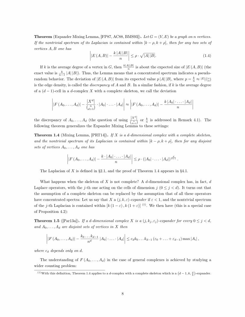
is the edge density, is called the discrepancy of A and B. In a similar fashion, if k is the average degreeof a (d− 1)-cell in a d-complex X with a complete skeleton, we call the deviation∣∣∣∣∣|F (A0, . . . , Ad)| −

∣∣Xd∣∣(

nd+1

) · |A0| · . . . · |Ad|

∣∣∣∣∣ ≈∣∣∣∣|F (A0, . . . , Ad)| −

k |A0| · . . . · |Ad|n

∣∣∣∣the discrepancy of A0, . . . , Ad (the question of using |X

d|( nd+1)

or kn is addressed in Remark 4.1). The

following theorem generalizes the Expander Mixing Lemma to these settings:

Theorem 1.4 (Mixing Lemma, [PRT14]). If X is a d-dimensional complex with a complete skeleton,and the nontrivial spectrum of its Laplacian is contained within [k − ρ, k + ρ], then for any disjointsets of vertices A0, . . . , Ad one has∣∣∣∣|F (A0, . . . , Ad)| −

k · |A0| · . . . · |Ad|n

∣∣∣∣ ≤ ρ · (|A0| · . . . · |Ad|)dd+1 .

The Laplacian of X is defined in §2.1, and the proof of Theorem 1.4 appears in §4.1.

What happens when the skeleton of X is not complete? A d-dimensional complex has, in fact, dLaplace operators, with the j-th one acting on the cells of dimension j (0 ≤ j < d). It turns out thatthe assumption of a complete skeleton can be replaced by the assumption that of all these operatorshave concentrated spectra: Let us say that X a (j, k, ε)-expander if ε < 1, and the nontrivial spectrumof the j-th Laplacian is contained within [k (1− ε) , k (1 + ε)] (†). We then have (this is a special caseof Proposition 4.2):

Theorem 1.5 ([Par13a]). If a d-dimensional complex X is a (j, kj , εj)-expander for every 0 ≤ j < d,and A0, . . . , Ad are disjoint sets of vertices in X then∣∣∣∣|F (A0, . . . , Ad)| −

k0 . . . kd−1

nd|A0| · . . . · |Ad|

∣∣∣∣ ≤ cdk0 . . . kd−1 (ε0 + . . .+ εd−1) max |Ai| ,

where cd depends only on d.

The understanding of F (A0, . . . , Ad) in the case of general complexes is achieved by studying awider counting problem:

(†)With this definition, Theorem 1.4 applies to a d-complex with a complete skeleton which is a(d− 1, k, ρ

k

)-expander.

8

Definition 1.6. Given disjoint sets A0, . . . , A` ⊆ V , and j ≤ `, a j-gallery in A0, . . . , A` is a se-quence of j-cells σ0, . . . , σ`−j ∈ Xj , such that σi is in F (Ai, . . . , Ai+j), and σi and σi+1 intersect in a(j − 1)-cell (which must lie in F (Ai+1, . . . , Ai+j)). We denote the set of j-galleries in A0, . . . , A` byF j (A0, . . . , A`).

Example.

(1) An `-gallery in A0, . . . , A` is just a single `-cell, so that F ` (A0, . . . , A`) = F (A0, . . . , A`).

(2) A 0-gallery is any sequence of vertices, so that F 0 (A0, . . . , A`) = A0 × . . .×A`.

(3) F 2 (A,B,C,D,E) is the number of triplets of triangles t1 ∈ F (A,B,C), t2 ∈ F (B,C,D),t3 ∈ F (C,D,E) such that the boundaries of t1 and t2 share a common edge (necessarily inF (B,C)), and likewise for t2 and t3.

The heart of our analysis is the following lemma, which estimates the size of F j+1 (A0, . . . , A`)

in terms of that of F j (A0, . . . , A`). Repeatedly applying this lemma allows us to estimate|F (A0, . . . , Ad)| =

∣∣F d (A0, . . . , Ad)∣∣ in terms of

∣∣F 0 (A0, . . . , Ad)∣∣ = |A0| · . . . · |Ad|.

Lemma 1.7 (Descent Lemma, [Par13a]). Let A0, . . . , A` be disjoint sets of vertices in X. If X is an(i, ki, εi)-expander for i = j − 1, i = j, then

∣∣∣∣∣∣∣F j+1 (A0, . . . , A`)∣∣− ( kj

kj−1

)`−j ∣∣F j (A0, . . . , A`)∣∣∣∣∣∣∣

≤ (`− j) k`−jj (εj + εj−1)√|F (A0, . . . , Aj)| |F (A`−j , . . . , A`)|.

The proofs of this lemma and of the mixing lemma it implies (Theorem 1.5) appear in §4.2.

1.3 Examples and applications

If a graph G = (V,E) has a large Cheeger constant, then given a mapping ϕ : V → R, there existsa point x ∈ R which is covered by many edges in the linear extension of ϕ to E (namely, x =

median (ϕ (v) | v ∈ V ). This observation led Gromov to define the geometric overlap of a complex([Gro10], see also [FGL+12, MW11]):

Definition 1.8. Let X be a d-dimensional simplicial complex. The overlap of X is defined by

overlap (X) = minϕ:V→Rd

maxx∈Rd

#σ ∈ Xd

∣∣x ∈ conv ϕ (v) | v ∈ σ

|Xd|.

In other words, X has overlap ≥ ε if for every simplicial mapping of X into Rd (a mapping inducedlinearly by the images of the vertices), some point in Rd is covered by at least an ε-fraction of thed-cells of X.

A theorem of Pach [Pac98], together with our mixing Lemmas yield a connection between thespectrum of the Laplacian and the overlap property:

9

Proposition. There exist positive constants Cd and C ′d with the following property: if a d-complex Xis a (j, kj , εj)-expander for 0 ≤ j < d then

overlapX > Cd − C ′d (ε0 + . . .+ εd−1) .

Corollary 5.2 proves this for complexes with a complete skeleton, and Proposition 5.4 for the generalcase. As an application, we show that Linial-Meshulam complexes have geometric overlap for suitableparameters:

Corollary. There exist ϑ > 0 such that for large enough C a.a.s. overlap(X(d, n, C·logn

n

))> ϑ.

This is a part of Corollary 5.7, which is proved in §5.4. Another application of the expander mixinglemma is bounding the chromatic number of a complex, defined in §5.2:

Proposition 1.9. There exists a constant Cd with the following property: if a d-complex X is a(j, kj , εj)-expander for 0 ≤ j < d then

χ (X) ≥ Cdd√ε0 + . . .+ εd−1

,

where χ (X) is the chromatic number of X.

The Ramanujan graphs constructed in [LPS88, Mar88] form a celebrated example of excellentexpanders. Their construction and study was generalized to Ramanujan complexes in [CSŻ03, Li04,LSV05a, LSV05b], but as of now little is known on their combinatorial expansion. In §5.5, which isbased on [GP13], we study the Hodge spectrum of Ramanujan triangle complexes, i.e. complexes ofdimension two. We obtain the following isoperimetric bound (for the definitions see §5.5):

Theorem 1.10. If X is a non-3-colorable Ramanujan triangle complex with n vertices, vertex degreek0 = 2

(q2 + q + 1

)and edge degree k1 = q + 1, then

|F (A,B,C)||A| |B| |C|

≥ 1

n2(q + 1− 2

√q)

(2q2 + 2q + 2− 6q

(1 +

10

9 |A| |B| |C|

))holds for any partition V (X) = A

∐B∐C.

This can be stated in terms of an appropriate Cheeger constant (see (5.10) and (5.11)). Further-more, we show that the major part of the spectrum of X is concentrated, giving hope of establishingpseudo-randomness in the future.

1.4 High dimensional random walk

There are well known connections between dynamical, topological and spectral properties of graphs:The random walk on a graph reflects both its topological and algebraic connectivity, which are reflectedby the 0th-homology and the spectral gap, respectively. In §6 we present a stochastic process whichgeneralizes these connections to higher dimensions. In particular, for a finite d-dimensional complex,the asymptotic behavior of the process reflects the existence of a nontrivial (d− 1)-homology, and its

10

rate of convergence is dictated by the normalized spectral gap (see §6.2). In order to give a flavorof the results without plunging into the most general definitions, we present here, without proofs thespecial case of regular triangle complexes.

First, let us observe the 12 -lazy random walk on a k-regular graph G = (V,E): the walker starts at

a vertex v0, and at each step remains in place with probability 12 or moves to each of its k neighbors

with probability 12k . Let pv0n (v) denote the probability of finding the walker at the vertex v at time

n. The following observations are classic:

(1) If G is finite, then pv0∞ = limn→∞ pv0n exists, and it is constant if and only if G is connected.

(2) Furthermore, the rate of convergence is given by

‖pv0n − const‖ = O

((1− 1

2λ (G)

)n),

where λ (G) is the spectral gap of G (the definition follows below).

(3) When G is infinite and connected, the spectral gap is related to the return probability of thewalk by

limn→∞

n√pv0n (v0) = 1− 1

2λ (G) . (1.5)

Let us denote in this section by ∆+ the normalized Laplacian of G, which acts on RV by

(∆+f

)(v) = f (v)− 1

k

∑w∼v

f (w)

If G is finite, then its spectral gap λ (G) is the minimal Laplacian eigenvalue on a function whose sumon V vanishes. When G is infinite, its spectral gap is defined to be λ (G) = min Spec

(∆+∣∣L2(V )

)(for

more on this see §7.1).

Moving one dimension higher, let X = (V,E, T ) be a k-regular triangle complex, namely every edgein E = X1 is contained in exactly k triangles in T = X2. For v, w ∈ E we denote the directed edgev• // w• by [v, w], and the set of all directed edges by E± (so that |E±| = 2 |E|). For e ∈ E±, e denotesthe edge with the same vertices and opposite direction, i.e. [v, w] = [w, v].

The following definition is the basis of the process which we shall study:

Definition 1.11. Two directed edges e, e′ ∈ E± are called neighbors (indicated by e ∼ e′) if theyhave the same origin or the same terminus, and the triangle they form is in the complex. Namely, ife = [v, w] and e′ = [v′, w′], then e ∼ e′ means that either v = v′ and v, w,w′ ∈ T , or w = w′ andv, v′, w′ ∈ T .

We study the following lazy random walk on E±: The walk starts at some directed edge e0 ∈ E±.At every step, the walker stays put with probability 1

2 , or else move to a uniformly chosen neighbor.Figure 1.1 illustrates one step of the process, in two cases (the right one is non-regular, but the walkis defined in the same manner).

As in the random walk on a graph, this process induces a sequence of distributions on E±,

pn (e) = pe0n (e) ,

11

Figure 1.1: One step of the edge walk.

describing the probability of finding the walker at the directed edge e at time n (having started frome0). However, studying the evolution of pn amounts to studying the traditional random walk on thegraph with vertices E± and edges defined by ∼. This will not take us very far, and in particular willnot reveal the presence or absence of first homology in X. Instead, we study the evolution of what wecall the “expectation process” on X:

En (e) = Ee0n (e) = pe0n (e)− pe0n (e) ,

i.e. the probability of finding the walker at time n at e, minus the probability of finding it at theopposite edge e (for the reasons behind the name see Remark 6.4).

It is tempting to look at Ee0∞ = limn→∞ Ee0n as is done in graphs, but a moment of reflection willshow the reader that Ee0∞ ≡ 0 for any finite triangle complex, and any starting point e0. Namely, theprobabilities of reaching e and e become arbitrarily close, for every e. While this might cause initialworry, it turns out that the rate of decay of En is always the same: for any finite triangle complex onehas ‖Ee0n ‖ = Θ

((34

)n). It is therefore reasonable to turn our attention to the normalized expectationprocess,

Ee0n (e) =(

43

)n Ee0n (e) =(

43

)n [pe0n (e)− pe0n (e)

],

and observe its limit,Ee0∞ = lim

n→∞Ee0n .

For a finite triangle complex this limit always exists, and is nonzero. This is the object which reveals thefirst homology of the complex. To see how, we need the following definition: We say that f : E± → Ris exact if its sum along every closed path vanishes; namely, if

v0 ∼ v1 ∼ . . . ∼ vn = v0 =⇒n−1∑i=0

f ([vi, vi+1]) = 0.

This is the one-dimensional analogue of constant functions (for reasons which will become clear in §2),and the following holds:

(1) For a finite X, Ee0∞ is exact for every e0 ∈ E± if and only if G has a trivial first homology.

12

(2) Furthermore, the rate of convergence is given by

∥∥∥Ee0n − exact∥∥∥ = O

((1− 1

3λ (X)

)n),

where λ (X) is the spectral gap of X (see §6.2).

(3) If X is infinite and every vertex in X is of infinite degree, then its spectral gap (which is definedin §7.2) is revealed by the “return expectation”:

supe0∈E±

limn→∞

n

√Ee0n (e0) = 1− 1

3λ (X) .

What if one is interested not only in the existence of a first homology, but also in its dimension? Theanswer is manifested in the walk as well. In graphs the number of connected components is given bythe dimension of Span pv0∞ | v0 ∈ V , and an analogue statement holds here (see Theorem 6.9).

Remark. If the non-lazy walk on a finite graph is observed, then apart from disconnectedness there isanother obstruction for convergence to the uniform distribution: bipartiteness. We shall see that thisis a special case of an obstruction in general dimension, which we call disorientability (see Definition6.6). In our example we have avoided this problem by considering the lazy walk, both on graphs andon triangle complexes.

The analogue process for general dimension, and for non-regular complexes, is defined in §6.1. In§6.3 we define the corresponding normalized expectation process Eσ0

n . In §6.3 it is shown that the limitof this process Eσ0

∞ = limn Eσ0n always exists and captures various properties of X, according to the

amount of laziness p (this is an abridged version of Theorem 6.9):

Theorem. When d−13d−1 < p < 1, Eσ0

∞ is exact for every starting point σ0 if and only if the (d− 1)-homology of X is trivial. If furthermore p ≥ 1

2 then the rate of convergence is controlled by the spectralgap of X:

dist(Eσ0n , Eσ0

∞

)= O

((1− 1− p

p (d− 1) + 1λ (X)

)n).

When p = d−13d−1 , E

σ0∞ is exact for every starting point σ0 if and only if the (d− 1)-homology of X is

trivial, and in addition X has no disorientable (d− 1)-components (see Definitions 6.2, 6.6).

1.5 Infinite complexes

In §7 we we turn to infinite complexes, studying the high-dimensional analogues of classic propertiesand theorems regarding infinite graphs. In this study we encounter new phenomena along the familiarones, which reveal that graphs present only a degenerated case of a broader theory.

In §7.3 we define a family of simplicial complexes (which we call arboreal complexes) generalizingthe notion of trees. In Theorem 7.3 we compute their spectra, extending Kesten’s classic result on thespectrum of regular trees [Kes59]. The spectra of the regular arboreal complexes of high dimensionand low regularity exhibit a surprising new phenomenon - an isolated eigenvalue.

Sections 7.4 and 7.5 are devoted to study the behavior of the spectrum with respect to a limitin the space of complexes. In particular we are interested in the high-dimensional analogue of the

13

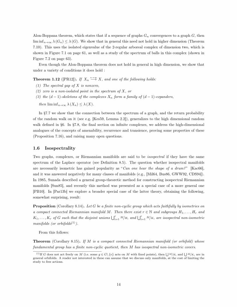
Alon-Boppana theorem, which states that if a sequence of graphs Gn convergences to a graph G, thenlim infn→∞ λ (Gn) ≤ λ (G). We show that in general this need not hold in higher dimension (Theorem7.10). This uses the isolated eigenvalue of the 2-regular arboreal complex of dimension two, which isshown in Figure 7.1 on page 61, as well as a study of the spectrum of balls in this complex (shown inFigure 7.2 on page 63).

Even though the Alon-Boppana theorem does not hold in general in high dimension, we show thatunder a variety of conditions it does hold :

Theorem 1.12 ([PR12]). If Xnn→∞−→ X, and one of the following holds:

(1) The spectral gap of X is nonzero,(2) zero is a non-isolated point in the spectrum of X, or(3) the (d− 1)-skeletons of the complexes Xn form a family of (d− 1)-expanders,

then lim infn→∞ λ (Xn) ≤ λ (X).

In §7.7 we show that the connection between the spectrum of a graph, and the return probabilityof the random walk on it (see e.g. [Kes59, Lemma 2.2]), generalizes to the high dimensional randomwalk defined in §6. In §7.8, the final section on infinite complexes, we address the high-dimensionalanalogues of the concepts of amenability, recurrence and transience, proving some properties of these(Proposition 7.16), and raising many open questions.

1.6 Isospectrality

Two graphs, complexes, or Riemannian manifolds are said to be isospectral if they have the samespectrum of the Laplace operator (see Definition 8.5). The question whether isospectral manifoldsare necessarily isometric has gained popularity as “Can one hear the shape of a drum? ” [Kac66],and it was answered negatively for many classes of manifolds (e.g., [Mil64, Bus86, GWW92, CDS94]).In 1985, Sunada described a general group-theoretic method for constructing isospectral Riemannianmanifolds [Sun85], and recently this method was presented as a special case of a more general one[PB10]. In [Par13b] we explore a broader special case of the latter theory, obtaining the following,somewhat surprising, result:

Proposition (Corollary 8.14). Let G be a finite non-cyclic group which acts faithfully by isometries ona compact connected Riemannian manifold M . Then there exist r ∈ N and subgroups H1, . . . ,Hr andK1, . . . ,Kr of G such that the disjoint unions

⋃ri=1

M/Hi and⋃ri=1

M/Ki are isospectral non-isometricmanifolds (or orbifolds(†)).

From this follows:

Theorem (Corollary 8.15). If M is a compact connected Riemannian manifold (or orbifold) whosefundamental group has a finite non-cyclic quotient, then M has isospectral non-isometric covers.

(†)If G does not act freely on M (i.e. some g ∈ G\ e acts on M with fixed points), then⋃M/Hi and

⋃M/Ki are in

general orbifolds. A reader not interested in these can assume that we discuss only manifolds, at the cost of limiting thestudy to free actions.

14

Let M denote a compact Riemannian manifold, and let G be a finite group which acts on it byisometries. In these settings, Sunada’s theorem [Sun85] states that if two subgroups H,K ≤ G satisfy

∀g ∈ G : |[g] ∩H| = |[g] ∩K| , (1.6)

where [g] denotes the conjugacy class of g in G, then the quotients M/H and M/K are isospectral. Infact, it is not harder to show (see Corollary 8.6) that if two collections H1, . . . ,Hr and K1, . . . ,Kr ofsubgroups of G satisfy

∀g ∈ G :

r∑i=1

|[g] ∩Hi||Hi|

=

r∑i=1

|[g] ∩Ki||Ki|

(1.7)

then⋃M/Hi and

⋃M/Ki are isospectral(†). We shall see, however, that in contrast with Sunada pairs

(H,K satisfying (1.6)), collections satisfying (1.7) are rather abundant. In fact, we will show thatevery finite non-cyclic group G has such collections, and furthermore, that some of them (which wedenote unbalanced, see Definition 8.7) necessarily yield non-isometric quotients.

1.6.1 Example

Let T be the torus R2/Z2. Let G = e, σ, τ, στ be the non-cyclic group of size four (i.e. G ∼= Z/2Z×Z/2Z),

and let σ, τ ∈ G act on T by rotations: σ · (x, y) =(x, y + 1

2

)and τ · (x, y) =

(x+ 1

2 , y)(Figure 1.2).

Figure 1.2: Two views of an action ofG = e, σ, τ, στ ∼= Z/2Z × Z/2Z on thetorus T .

The subgroups

H1 = e, σH2 = e, τH3 = e, στ

K1 = eK2 = K3 = G

(1.8)

satisfy (1.7): since G is abelian, (1.7) becomes ∀g ∈ G :∑

i : g∈Hi

1|Hi| =

∑i : g∈Ki

1|Ki| , which is easy

to verify. Thus, the unions of tori⋃T/Hi = T/〈σ〉

⋃T/〈τ〉

⋃T/〈στ〉 and

⋃T/Ki = T

⋃T/G

⋃T/G are

isospectral (Figure 1.3).

Figure 1.3: An isospectral pair consisting of quotients of the torus T (Figure 1.2) by the subgroups ofG described in (1.8).

(†)In what follows⋃

always stands for disjoint union.

15

2 Preliminaries

Throughout this work X denotes a finite d-dimensional simplicial complex with vertex set V of size n(with n < ∞ until §7), and Xj denotes the set of j-cells of X, where −1 ≤ j ≤ d. In particular, wehave X−1 = ∅. For j ≥ 1, every j-cell σ = σ0, . . . , σj has two possible orientations, correspondingto the possible orderings of its vertices, up to an even permutation (1-cells and the empty cell haveonly one orientation). We denote an oriented cell by square brackets, and a flip of orientation by anoverbar. For example, one orientation of σ = x, y, z is [x, y, z], which is the same as [y, z, x] and[z, x, y]. The other orientation of σ is [x, y, z] = [y, x, z] = [x, z, y] = [z, y, x]. We denote by Xj

± the setof oriented j-cells (so that

∣∣∣Xj±

∣∣∣ = 2∣∣Xj

∣∣ for j ≥ 1 and Xj± = Xj for j = −1, 0).

We now describe the so-called simplicial Hodge theory, due to Eckmann [Eck44]. This is a discreteanalogue of Hodge theory in Riemannian geometry, but in contrast, the proofs of the statements areall exercises in finite-dimensional linear algebra. Furthermore, it applies to any complex, and not onlyto manifolds.

The space of j-forms on X, denoted Ωj (X), is the vector space of skew-symmetric functions onoriented j-cells:

Ωj = Ωj (X) =f : Xj

± → R∣∣∣ f (σ) = −f (σ) ∀σ ∈ Xj

±

.

In particular, Ω0 is the space of functions on V , and Ω−1 = R∅ can be identified in a natural waywith R. With every oriented j-cell σ ∈ Xj we associate the Dirac j-form 1σ defined by

1σ (σ′) =

1 σ′ = σ

−1 σ′ = σ

0 otherwise

(for j = 0 this is the standard Dirac function, and 1∅ is the constant 1).For a cell σ (either oriented or non-oriented) and a vertex v, we write v/σ if v /∈ σ and v∪σ is a cell

inX. If σ = [σ0, . . . , σj ] is oriented and v/σ, then vσ denotes the oriented (j + 1)-cell [v, σ0, . . . , σj ]. Anoriented j-cell [σ0, . . . , σj ] induces orientations on its faces - the (j − 1)-cells which form its boundary- as follows: the face σ0, . . . , σi−1, σi+1, . . . , σj is oriented as (−1)

i[σ0, . . . , σi−1, σi+1, . . . , σj ], where

(−1) τ = τ .(†)

The jth boundary operator ∂j : Ωj → Ωj−1 is

(∂jf) (σ) =∑v/σ

f (vσ) ,

and in particular, ∂0 : Ω0 → Ω−1 is defined by (∂0f) (∅) =∑v∈X0 f(v). The sequence (Ω•, ∂•) is a

(†)An edge e = [v0, v1] induces a “negative orientation” on v0. We do not bother to make this formal, as everythingwe study is well known and understood in dimension zero.

16

chain complex, i.e., ∂j−1∂j = 0 for all j, and one denotes

Zj = ker ∂j j-cycles

Bj = im ∂j+1 j-boundaries

Hj = Zj/Bj the jth homology of X(over R).

The notions presented so far go back to the nineteenth century; Eckmann’s innovation was introducinga “simplicial Riemannian structure”, by endowing each space Ωj with an inner product. Until §6, weassume that X is a finite complex and work with inner product

〈f, g〉 =∑σ∈Xj

f (σ) g (σ) (2.1)

(note that f (σ) g (σ) is well defined even without choosing an orientation for σ). In §6 we will choosea different inner product (see §6.2), which is better suited to analyze the stochastic process studiedthere. Section §7 treats infinite complexes, for which the situation is more involved, and most of thestatements to follow in this section are false. The proper adjustments are addressed in §7.2.

As Ωj and Ωj−1 are finite dimensional inner product spaces, ∂j has an adjoint operator. This isthe differential, or coboundary operator δj = ∂∗j : Ωj−1 → Ωj , given by

(∂∗j f

)(σ) =

∑τ is a

face of σ

f (τ) =

j∑i=0

(−1)if (σ\σi) ,

where σ\σi = [σ0, σ1, . . . , σi−1, σi+1, . . . σj ]. Here the standard terms are

Zj = ker ∂∗j+1 = B⊥j closed j-forms (or cocycles)

Bj = im ∂∗j = Z⊥j exact j-forms (or coboundaries)

Hj = Zj/Bj the jth cohomology of X(over R).

Example. For j = 0, Z0 consists of the locally constant functions (functions constant on connectedcomponents); B0 consists of the constant functions; Z0 of the functions whose sum vanishes, and B0

of the functions whose sum on each connected component vanishes.For j = 1, Z1 are the forms whose sum along the boundary of every triangle in the complex

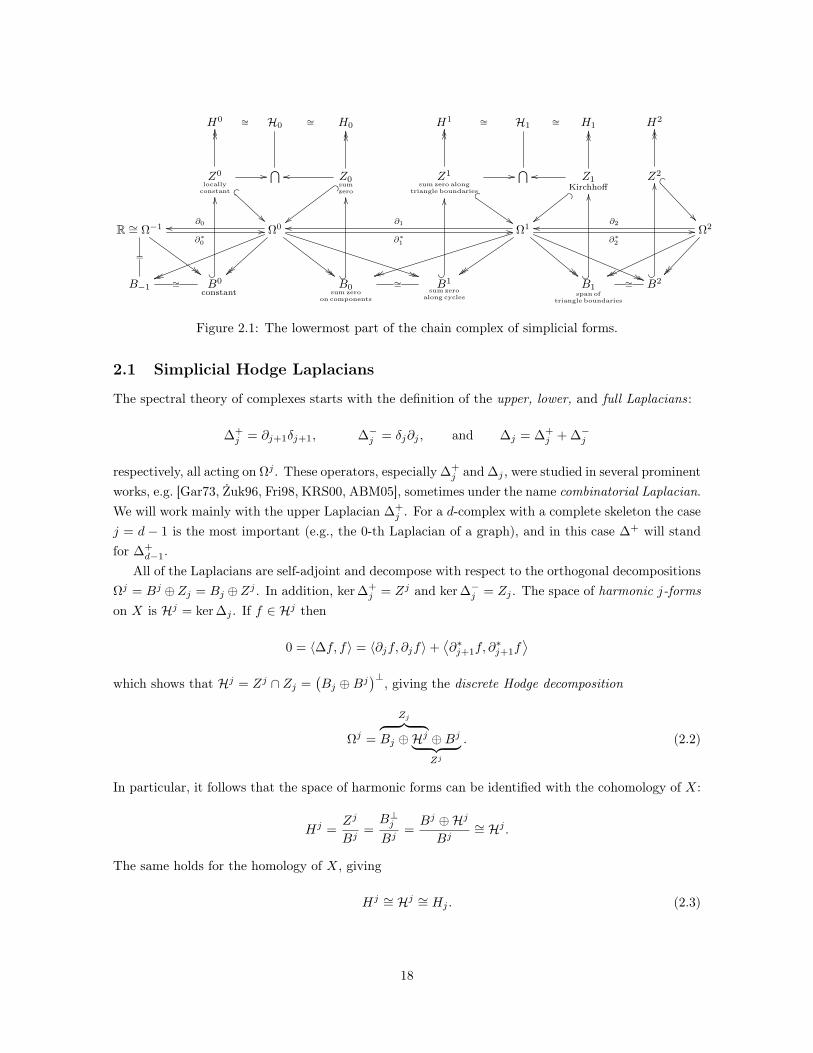
vanishes; in B1 lie the forms whose sum along every closed path vanishes; Z1 are the Kirchhoff forms,also known as flows, those for which the sum over all edges incident to a vertex, oriented inward, iszero; and B1 are the forms spanned (over R) by oriented boundaries of triangles in the complex. Thechain of simplicial forms in dimensions −1 to 2 is depicted in Figure 2.1.

17

H0 ∼= H0∼= H0 H1 ∼= H1

∼= H1 H2

Z0

locallyconstant

OOOO

p

!!

// ⋂ Z0sumzero

OOOO

oomM

Z1

sum zero alongtriangle boundaries

OOOO

r

$$

// ⋂ Z1Kirchhoff

OOOO

oo

mM

||

Z2

OOOO

n

R ∼= Ω−1

=

∂∗0

//

## ##

Ω0

## ## ** **uuuu

∂0oo∂∗1

// Ω1

zzzz "" ""tttt (( ((

∂1oo∂∗2

// Ω2

vvvv

∂2oo

B−1 B0

constant

?

OO

∼= B0sum zero

on components

?

OO

∼= B1sum zero

along cycles

?

OO

B1span of

triangle boundaries

?

OO

∼= B2?

OO

Figure 2.1: The lowermost part of the chain complex of simplicial forms.

2.1 Simplicial Hodge Laplacians

The spectral theory of complexes starts with the definition of the upper, lower, and full Laplacians:

∆+j = ∂j+1δj+1, ∆−j = δj∂j , and ∆j = ∆+

j + ∆−j

respectively, all acting on Ωj . These operators, especially ∆+j and ∆j , were studied in several prominent

works, e.g. [Gar73, Żuk96, Fri98, KRS00, ABM05], sometimes under the name combinatorial Laplacian.We will work mainly with the upper Laplacian ∆+

j . For a d-complex with a complete skeleton the casej = d − 1 is the most important (e.g., the 0-th Laplacian of a graph), and in this case ∆+ will standfor ∆+

d−1.All of the Laplacians are self-adjoint and decompose with respect to the orthogonal decompositions

Ωj = Bj ⊕Zj = Bj ⊕Zj . In addition, ker ∆+j = Zj and ker ∆−j = Zj . The space of harmonic j-forms

on X is Hj = ker ∆j . If f ∈ Hj then

0 = 〈∆f, f〉 = 〈∂jf, ∂jf〉+⟨∂∗j+1f, ∂

∗j+1f

⟩which shows that Hj = Zj ∩ Zj =

(Bj ⊕Bj

)⊥, giving the discrete Hodge decomposition

Ωj =

Zj︷ ︸︸ ︷Bj ⊕Hj ⊕Bj︸ ︷︷ ︸

Zj

. (2.2)

In particular, it follows that the space of harmonic forms can be identified with the cohomology of X:

Hj =Zj

Bj=B⊥jBj

=Bj ⊕Hj

Bj∼= Hj .

The same holds for the homology of X, giving

Hj ∼= Hj ∼= Hj . (2.3)

18

The dimension of ker ∆j∼= Hj

∼= Hj is the jth (reduced) Betti number of X, denoted by βj .

Remark. For comparison, the original Hodge decomposition states that for a Riemannian manifold Mand 0 ≤ j ≤ dimM , there is an orthogonal decomposition

Ωj (M) = d(Ωj−1 (M)

)⊕Hj (M)⊕ δ

(Ωj+1 (M)

)where Ωj are the smooth j-forms on M , d is the exterior derivative, δ its Hodge dual, and Hj thesmooth harmonic j-forms on M . As in the discrete case, this gives an isomorphism between the jth

de-Rham cohomology of M and the space of harmonic j-forms on it.

The combinatorial meaning of the Laplacians is better understood via the following adjacencyrelations on oriented cells:

Definition 2.1. Let σ and σ′ be two distinct oriented j-cells in X.

(1) We denote σ t σ′ if σ and σ′ intersect in a common (j − 1)-cell and induce the same orientationon it; for edges this means that they have a common origin or a common endpoint, and forvertices v t v′ holds whenever v 6= v′.

(2) We denote σ ∼ σ′, and say that σ and σ′ are neighbors, if σ t σ′, and in addition the (j + 1)-cellσ ∪ σ′ is in X. For vertices this is the common relation of neighbors in a graph.

Using these relations, the Laplacians can be expressed as follows (recall that the degree of a j-cellis the number of (j + 1)-cells in which it is contained):(

∆+j ϕ)

(σ) = deg (σ)ϕ (σ)−∑σ′∼σ

ϕ (σ′)

(∆−j ϕ

)(σ) = (j + 1)ϕ (σ) +

∑σ′tσ

ϕ (σ′)

(∆jϕ) (σ) = (deg σ + j + 1)ϕ (σ) +∑σ′tσσ′σ

ϕ (σ′)

(2.4)

We also define adjacency operators on Ωj which correspond to the ∼ and t relations:

(A∼j ϕ

)(σ) =

∑σ′∼σ

ϕ (σ′) ,(Atj ϕ)

(σ) =∑σ′tσ

ϕ (σ′) , (2.5)

so that ∆−j = (j + 1) · I + Atj and ∆+

j = Dj − A∼j , where Dj is the degree operator (Djf) (σ) =

deg (σ) f (σ).

2.2 The spectrum of complexes

The spectra we are primarily interested in are those of ∆+j for 0 ≤ j < d.(†) For j = 0, this is the

standard graph Laplacian (∆+

0 f)

(v) = deg (v) f (v)−∑v′∼v

f (v′) .

(†)It is sometimes useful to consider the Laplacian ∆+−1 as well. This operator acts on Ω−1 ∼= R as multiplication by

deg∅ = |V | = n, so that Spec ∆+−1 = n.

19

Every graph has a “trivial zero” in the spectrum of its Laplacian, corresponding to the constantfunctions, i.e. B0. Similarly, since (Ω•, δ•) is a co-chain complex, Bj = im δj is always contained inthe kernel of ∆+

j = ∂j+1δj+1, and the eigenvalues which correspond to forms in Bj are considered to

be the trivial spectrum of ∆+j . As

(Bj)⊥

= Zj , this leads to the following definition:

Definition 2.2. The nontrivial spectrum of ∆+j is Spec ∆+

j

∣∣Zj, and the j-dimensional spectral gap,

denoted λj (X), is the minimal nontrivial eigenvalue of ∆+j :

λ (X) = min Spec(

∆+j

∣∣Zj

)(Note that we also have λj (X) = min Spec

(∆j

∣∣Zj

)since ∆j

∣∣Zj≡ ∆+

j

∣∣Zj.)

Zero is a nontrivial eigenvalue of ∆+j (i.e. λj (X) = 0) precisely when Hj = Zj ∩ Zj 6= 0, which

by (2.3) happens iff X has nontrivial j-th homology. For example, the nontrivial spectrum of ∆+0

corresponds to Z0, which are the functions whose sum on all vertices vanish, and zero is a nontrivialeigenvalue of ∆+

0 iff the complex is disconnected.Since λj (X) = 0 indicates a non-trivial j-th homology, a large value of λj (X) should indicate a

“very trivial j-th homology”. For example, a graph with a large spectral gap should be “very connected”.The Cheeger inequality for graphs gives precise meaning to this intuition, and our ambition is togeneralize this to higher dimensions.

2.3 Complexes with a complete skeleton

Complexes with a complete skeleton appear to be particularly well behaved, in comparison with the gen-eral case. For these complexes we are mainly interested in λd−1,∆

+d−1,∆

−d−1,∆d−1, Dd−1,A∼d−1,At

d−1,and we denote them simply by λ,∆+, . . . (this will be the case until §4.2, and again in §6 and §7).

The following proposition lists some observations regarding these complexes. These will be used inthe proofs of the main theorems in §3, §4.1, and also to obtain simpler characterizations of the spectralgap in this case.

Proposition 2.3. If X has a complete skeleton, then

(1) If X is the complement complex of X, i.e., Xd−1

= Xd−1 =(Vd

)(†) and X

d=(Vd+1

)\Xd, then

∆+

X= n · I −∆X . (2.6)

(2) The spectrum of ∆ lies in the interval [0, n].

(3) The lower Laplacian of X satisfies∆− = n · PBd−1 (2.7)

where PBd−1 is the orthogonal projection onto Bd−1.(†) (V

j

)denotes the set of subsets of V of size j.

20

Proof. By (2.4) we have (∆Xf) (σ) = (deg σ + d) f (σ) +∑

σ′tσσ′σ

f (σ′), and as σ′ ∼ σ in X iff σ′ t σand σ′ σ in X, (

∆+

Xf)

(σ) = (n− d− deg (σ)) f (σ)−∑σ′tσσ′σ

f (σ′) ,

hence (1 ) follows. From (1 ) we conclude that Spec ∆+

X=n− γ

∣∣ γ ∈ Spec ∆X

, and since ∆X and

∆+

Xare positive semidefinite, (2 ) follows. To establish (3 ), recall that

(Bd−1

)⊥= Zd−1 = ker ∆−, and

it is left to show that ∆−f = nf for f ∈ Bd−1. Note that Bd−1 ⊆ Zd−1 = ker ∆+X , and in addition,

that since Bd−1 only depends on X’s (d− 1)-skeleton,

Bd−1 (X) = Bd−1(X)⊆ Zd−1

(X)

= ker ∆+

X.

Now from (1 ) it follows that for f ∈ Bd−1

∆−Xf = ∆−Xf + ∆+Xf = ∆Xf = nf −∆+

Xf = nf

as desired.

The following proposition gives several alternate characterizations of λ (X):

Proposition 2.4. Let λ (X) = λd−1 (X) be the (d− 1)-th spectral gap.

(1) λ (X) is the (r + 1)-th smallest eigenvalue of ∆+d−1, where r =

(∣∣Xd−1∣∣− βd−1

)−(∣∣Xd

∣∣− βd).Furthermore, if X has a complete skeleton, then

(2) λ (X) is the(n−1d−1

)+ 1 smallest eigenvalue of ∆+,

(3) andλ (X) = min Spec ∆. (2.8)

Remarks.

(1) For a graph G = (V,E) we have λ (G) = λr, where r = |V | − |E| − β0 + β1 = 1 (this followsfrom Euler’s formula), hence λ (G) is the second smallest eigenvalue of the graph’s Laplacian.

Alternatively, (2.8) gives λ (G) = min Spec (∆+ + J), where J = ∆− =

( 1 1 ··· 11 1 ··· 1....... . .

...1 1 ··· 1

).

(2) In general (2.8) does not hold: for example, for the triangle complex IJ, λ = min Spec(

∆∣∣Z1

)=

3 but min Spec ∆ = 1.

Proof.

(1) Since ∆+ decomposes w.r.t. Ωd−1 = Bd−1⊕Zd−1, and ∆+∣∣Bd−1 ≡ 0, the spectrum of ∆+ consists

of r = dimBd−1 zeros, followed by the spectral gap. To compute r, we observe that

dimBj−1 = dimZj−1 − dimHj−1 = null ∂∗j − βj−1

= dim Ωj−1 − rank ∂∗j − βj−1 =∣∣Xj−1

∣∣− dimBj − βj−1

21

and therefore

r = dimBd−1 =∣∣Xd−1

∣∣− dimBd − βd−1 =∣∣Xd−1

∣∣− (∣∣Xd∣∣− dimBd+1 − βd

)− βd−1

=(∣∣Xd−1

∣∣− βd−1

)−(∣∣Xd

∣∣− βd) .(2) The Euler characteristic satisfies

∑di=−1 (−1)

i ∣∣Xi∣∣ = χ (X) =

∑di=−1 (−1)

iβi. Therefore,

r =(∣∣Xd−1

∣∣− βd−1

)−(∣∣Xd

∣∣− βd)=(∣∣Xd−1

∣∣− βd−1

)−(∣∣Xd

∣∣− βd)+ (−1)d

d∑i=−1

(−1)i (∣∣Xi

∣∣− βi)=

d−2∑i=−1

(−1)d+i (∣∣Xi

∣∣− βi) .Since the (d− 1)-skeleton is complete,

∣∣Xi∣∣ =

(ni+1

)and βi = 0 for −1 ≤ i ≤ d− 2, and so

r =

d−2∑i=−1

(−1)d+i

(n

i+ 1

)=

(n− 1

d− 1

).

(3) First, since ∆ decomposes w.r.t. Ωd−1 = Bd−1 ⊕ Zd−1 we have

Spec ∆ = Spec ∆∣∣Bd−1 ∪ Spec ∆

∣∣Zd−1

= Spec ∆−∣∣Bd−1 ∪ Spec ∆+

∣∣Zd−1

.

By Proposition 2.3, Spec ∆−∣∣Bd−1 = n and Spec ∆ ⊆ [0, n], which implies that λ =

min Spec(

∆+∣∣Zd−1

)= min Spec ∆.

We finish with a note on the density of d-cells inX, which will come in handy later. A generalizationof this to complexes with a non-complete skeleton appears in Lemma 5.5.

Proposition 2.5. Let X be a d-complex with a complete skeleton. Let D denote the d-cell density

of X, D =|Xd|( nd+1)

, let k denote the average degree of a (d− 1)-cell, and let λavg denote the average

nontrivial eigenvalue of ∆+ = ∆+d−1. Then

D =λavgn

=k

n− d.

Proof. On the one hand,

D =

∣∣Xd∣∣(

nd+1

) =

∣∣Xd−1∣∣ kd+1(

nd+1

) =

(nd

)kd+1(nd+1

) =k

n− d.

22

On the other,(n

d

)k =

∣∣Xd−1∣∣ k =

∑σ∈Xd−1

deg σ = trace ∆+ =∑

λ∈Spec ∆+

λ =∑

λ∈Spec ∆+|Zd−1

λ,

and by Proposition 2.4

λavg =1(

nd

)−(n−1d−1

) ∑λ∈Spec ∆+|Zd−1

λ =1(n−1d

) ∑λ∈Spec ∆+|Zd−1

λ =n

n− d· k.

23

3 Isoperimetric constant

3.1 A Cheeger-type inequality

This section is devoted to the proof of Theorem 1.2: For a complex with a complete skeleton, the gen-eralized Cheeger constant (Definition 1.1) is bounded from below by the spectral gap (Definition 2.2).

Proof of Theorem 1.2. Recall that we seek to show

min Spec(

∆+∣∣Zd−1

)= λ (X) ≤ h (X) = min

V=∐di=0 Ai

n · |F (A0, A1, . . . , Ad)||A0| · |A1| · . . . · |Ad|

.

Let A0, . . . , Ad be a partition of V which realizes the minimum in h. We define f ∈ Ωd−1 by

f ([σ0 σ1 . . . σd−1]) =

sgn (π)∣∣Aπ(d)

∣∣ ∃π ∈ Sym0...d with σi ∈ Aπ(i) for 0 ≤ i ≤ d− 1

0 else, i.e. ∃k, i 6= j with σi, σj ∈ Ak.(3.1)

Note that f (π′σ) = sgn (π′) f (σ) for any π′ ∈ Sym0...d−1 and σ ∈ Xd−1. Therefore, f is a well-defined skew-symmetric function on oriented (d− 1)-cells, i.e., f ∈ Ωd−1. Figure 3.1 illustrates f ford = 1, 2.

A0 A1

A2

|A2|

|A0||A1|

0

00

0

0

Figure 3.1: The form f ∈ Ωd−1 defined in (3.1), for complexes of dimensions one and two.

We proceed to show that f ∈ Zd−1. Let σ = [σ0, σ1, . . . , σd−2] ∈ Xd−2± . As we assumed that Xd−1

is complete,

(∂d−1f) (σ) =∑v/σ

f ([v, σ0, σ1, . . . , σd−2]) =∑v/∈σ

f ([v, σ0, σ1, . . . , σd−2]) .

If for some k and i 6= j we have σi, σj ∈ Ak, this sum vanishes. On the other hand, if there existsπ ∈ Sym0...d such that σi ∈ Aπ(i) for 0 ≤ i ≤ d− 2 then

(∂d−1f) (σ) =∑

v∈Aπ(d−1)

f ([v, σ0, σ1, . . . , σd−2]) +∑

v∈Aπ(d)

f ([v, σ0, σ1, . . . , σd−2])

=∑

v∈Aπ(d−1)

(−1)d−1

sgnπ∣∣Aπ(d)

∣∣+∑v∈Ad

(−1)d

sgnπ∣∣Aπ(d−1)

∣∣= (−1)

d−1sgnπ

(∣∣Aπ(d−1)

∣∣ ∣∣Aπ(d)

∣∣− ∣∣Aπ(d)

∣∣ ∣∣Aπ(d−1)

∣∣) = 0

24

and in both cases f ∈ Zd−1. Thus, by Rayleigh’s principle

λ (X) = min Spec(

∆+∣∣Zd−1

)≤ 〈∆

+f, f〉〈f, f〉

=〈∂∗df, ∂∗df〉〈f, f〉

. (3.2)

The denominator is〈f, f〉 =

∑σ∈Xd−1

f (σ)2,

and a (d− 1)-cell σ contributes to this sum only if its vertices are in different blocks of the partition,i.e., there are no k and i 6= j with σi, σj ∈ Ak. In this case, there exists a unique block, Ai, whichdoes not contain a vertex of σ, and σ contributes |Ai|2 to the sum. Since Xd−1 is complete, there are|A0| · . . . · |Ai−1| · |Ai+1| · . . . · |Ad| non-oriented (d− 1)-cells whose vertices are in distinct blocks andwhich do not intersect Ai, hence

〈f, f〉 =

d∑i=0

∏j 6=i

|Aj |

|Ai|2 = n

d∏i=0

|Ai| .

To evaluate the numerator in (3.2), we first show that for σ ∈ Xd

|(∂∗df) (σ)| =

n σ ∈ F (A0, . . . , Ad)

0 σ /∈ F (A0, . . . , Ad) .(3.3)

First, let σ /∈ F (A0, . . . , Ad). If σ has three vertices from the same Ai, or two pairs of vertices fromthe same blocks (i.e. σi, σj ∈ Ak and σi′ , σj′ ∈ Ak′), then for every summand in

(∂∗df) (σ) =

d∑i=0

(−1)if (σ\σi) ,

the cell σ\σi has two vertices from the same block, and therefore (∂∗df) (σ) = 0. Next, assume thatσj and σk (with j < k) is the only pair of vertices in σ which belong to the same block. The onlynon-vanishing terms in (∂∗df) (σ) =

∑di=0 (−1)

if (σ\σi) are i = j and i = k, i.e.,

(∂∗df) (σ) = (−1)jf (σ\σj) + (−1)

kf (σ\σk) .

Since the value of f on a simplex depends only on the blocks to which its vertices belong,

f (σ\σj) = f ([σ0 σ1 . . . σj−1 σj+1 . . . σk−1 σk σk+1 . . . σd])

= f ([σ0 σ1 . . . σj−1 σj+1 . . . σk−1 σj σk+1 . . . σd])

= f(

(−1)k−j+1

[σ0 σ1 . . . σj−1 σj σj+1 . . . σk−1 σk+1 . . . σd])

= (−1)k−j+1

f (σ\σk) ,

so that(∂∗df) (σ) = (−1)

j(−1)

k−j+1f (σ\σk) + (−1)

kf (σ\σk) = 0.

25

The remaining case is σ ∈ F (A0, . . . , Ad). Here, there exists π ∈ Sym0...d with σi ∈ Aπ(i) for0 ≤ i ≤ d. Observe that

f (σ\σi) = sgn (π · (d d−1 d−2 . . . i))∣∣Aπ(i)

∣∣ = (−1)d−i

sgnπ∣∣Aπ(i)

∣∣and therefore

(∂∗df) (σ) =

d∑i=0

(−1)if (σ\σi) = (−1)

dsgnπ

d∑i=0

∣∣Aπ(i)

∣∣ = (−1)d

sgnπ · n.

Therefore, |(∂∗df) (σ)| = n. This establishes (3.3), which implies that

〈∂∗df, ∂∗df〉 =∑σ∈Xd

|(∂∗df) (σ)|2 = n2 |F (A0, . . . , Ad)|

and in totalλ (X) ≤ 〈∂

∗df, ∂

∗df〉

〈f, f〉=n |F (A0, . . . , Ad)|∏d

i=0 |Ai|= h (X) .

3.2 Towards a lower Cheeger inequality

The first observation to be made regarding a lower Cheeger inequality, is that no bound of the formC · h (X)

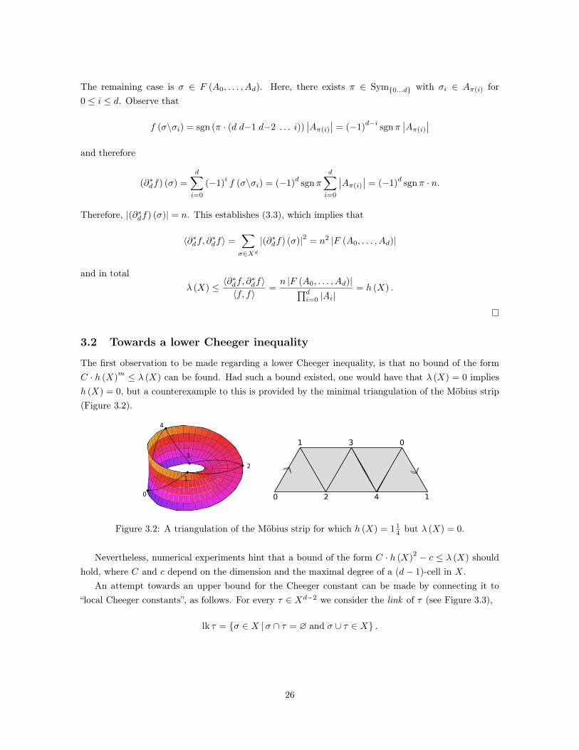
m ≤ λ (X) can be found. Had such a bound existed, one would have that λ (X) = 0 impliesh (X) = 0, but a counterexample to this is provided by the minimal triangulation of the Möbius strip(Figure 3.2).

1 3 0

0 2 4 1

Figure 3.2: A triangulation of the Möbius strip for which h (X) = 114 but λ (X) = 0.

Nevertheless, numerical experiments hint that a bound of the form C · h (X)2 − c ≤ λ (X) should

hold, where C and c depend on the dimension and the maximal degree of a (d− 1)-cell in X.An attempt towards an upper bound for the Cheeger constant can be made by connecting it to

“local Cheeger constants”, as follows. For every τ ∈ Xd−2 we consider the link of τ (see Figure 3.3),

lk τ = σ ∈ X |σ ∩ τ = ∅ and σ ∪ τ ∈ X .

26

Figure 3.3: Two examples for the link of a vertex in a triangle complex.

Since dim τ = d − 2, lk τ is a graph, and there is a 1 − 1 correspondence between vertices (edges)of lk τ and (d− 1)-cells (d-cells) of X which contain τ . We have the following bound for the Cheegerconstant of X:

Proposition 3.1. The bound h (X) ≤ h(lk τ)

1− d−1n

holds for any d-complex X and τ ∈ Xd−2.

Proof. Write τ = [τ0, τ1, . . . , τd−2] and denote Ai = τi for 0 ≤ i ≤ d− 2. Due to the correspondencebetween (lk τ)

j and cells in Xd−1+j containing τ ,

h (lk τ)def= min

B∐C=(lk τ)0

|Elk τ (B,C)| ·∣∣∣(lk τ)

0∣∣∣

|B| · |C|= minB

∐C=(lk τ)0

|F (A0, . . . , Ad−2, B,C)| ·∣∣∣(lk τ)

0∣∣∣

|B| · |C|.

Assume that the minimum is attained by B = B0 and C = C0. We define

Ad−1 = B0, Ad = V \

(d−1⋃i=0

Ai

).

Now A0, . . . , Ad is a partition of V , and

F (A0, . . . , Ad−2, B0, C0) = F (A0, . . . , Ad−2, Ad−1, Ad)

since no d-cell containing τ has a vertex in Ad\C0. In addition,∣∣∣(lk τ)0∣∣∣ |Ad|

n |C0|≥

∣∣∣(lk τ)0∣∣∣ |Ad| − |Ad−1| (|Ad| − |C0|)

n |C0|

=[n− (d− 1)− (|Ad| − |C0|)] |Ad| − |Ad−1| (|Ad| − |C0|)

n |C0|

=(n− (d− 1)) |Ad| − (|Ad−1|+ |Ad|) (|Ad| − |C0|)

n |C0|

=(n− (d− 1)) [|Ad| − (|Ad| − |C0|)]

n |C0|= 1− d− 1

n,

27

which implies

h (lk τ) =F (A0, . . . , Ad−2, Ad−1, Ad)

∣∣∣(lk τ)0∣∣∣

|B0| · |C0|=F (A0, . . . , Ad−2, Ad−1, Ad)n

|A0| · . . . · |Ad|·

∣∣∣(lk τ)0∣∣∣ |Ad|

n |C0|

≥ h (X) ·

∣∣∣(lk τ)0∣∣∣ |Ad|

n |C0|≥(

1− d− 1

n

)h (X) .

Since lk τ is a graph, its Cheeger constant can be bounded using the lower inequality in (1.1).We also note that the degree of a vertex in lk τ corresponds to the degree of a (d− 1)-cell in X, andtherefore (

1− d−1n

)28k

h2 (X) ≤ h (lk τ)2

8k≤ h (lk τ)

2

8kτ≤ λ (lk τ) (3.4)

where k is the maximal degree of a (d− 1)-cell in X, and kτ of a vertex in lk τ .We now see that a bound of the spectral gap of links by that of the complex would yield a lower

Cheeger inequality. Such a bound was discovered by Garland [Gar73], and was studied further byseveral authors [Żuk96, ABM05, GW12]. The following lemma appears in [GW12], for a normalizedversion of the Laplacian. We give here its form for the Laplacian we use.

Lemma 3.2 ([Gar73, GW12]). Let X be a d-dimensional simplicial complex. Given f ∈ Ωd−1, σ ∈Xd−1, τ ∈ Xd−2 define a function fτ : (lk τ)

0 → R by fτ (v) = f (vτ), and an operator ∆+τ :

Ωd−1 (X)→ Ωd−1 (X) by

(∆+τ f)

(σ) =

degτ (σ) f (σ)−

∑σ′∼στ⊆σ′

f (σ′) τ ⊂ σ

0 τ * σ

where degτ (σ) = # σ′ ∼ σ | τ ⊆ σ′ = deglk τ (σ\τ). The following then hold:

(1) ∆+ =(∑

τ∈Xd−2 ∆+τ

)− (d− 1)D.

(2) 〈∆+τ f, f〉 =

⟨∆+

lk τfτ , fτ⟩.

(3) If f ∈ Zd−1 then fτ ∈ Z0 (lk τ).

(4)∑τ∈Xd−2 〈fτ , fτ 〉 = d 〈f, f〉.

Proof. (1) By the definition of ∆+τ ,∑

τ∈Xd−2

∆+τ f (σ)− (d− 1)Df (σ) =

∑τ∈Xd−2

τ⊆σ

(degτ (σ) f (σ)−

∑σ′∼στ⊆σ′

f (σ′)

)− (d− 1) deg (σ) f (σ)

=

( ∑τ∈Xd−2

τ⊆σ

degτ (σ)− (d− 1) deg σf (σ)

)−

∑τ∈Xd−2

τ⊆σ

∑σ′∼στ⊆σ′

f (σ′)

= deg (σ) f (σ)−∑σ′∼σ

f (σ′) = ∆+f (σ) .

28

(2) Let f ∈ Ωd−1 and τ ∈ Xd−2. We first notice that (∆+τ f)τ = ∆+

lk τfτ , since(∆+τ f)τ

(v) =(∆+τ f)

(vτ) = degτ (vτ) f (vτ)−∑σ′∼vττ⊆σ′

f (σ′)

= degτ (vτ) f (vτ)−∑v′∼τv′τ∼vτ

f (v′τ) = deglk τ (v) fτ (v)−∑v′∼

lk τv

fτ (v′) = ∆+lk τfτ (v) .

Since (lk τ)0

= v ∈ V | v ∼ τ, this gives

⟨∆+

lk τfτ , fτ⟩

=⟨(

∆+τ f)τ, fτ⟩

=∑v∼τ

(∆+τ f)τ

(v) fτ (v) =∑v∼τ

(∆+τ f)

(vτ) f (vτ) =⟨∆+τ f, f

⟩where the last equality is since ∆+

τ f is supported on (d− 1)-cells containing τ .

(3) If f ∈ Zd−1 and τ ∈ Xd−2 then

(∂lk τ

0 fτ)

(∅) =∑

v∈(lk τ)0

fτ (v) =∑

v∈(lk τ)0

f (vτ) =∑v∼τ

f (vτ) = (∂d−1f) (τ) = 0

implies that fτ ∈ Z0 (lk τ).

(4) This is by∑τ∈Xd−2

〈fτ , fτ 〉 =∑

τ∈Xd−2

∑v∼τ

f2τ (v) =

∑τ∈Xd−2

∑v∼τ

f2 (vτ) = d∑

σ∈Xd−1

f2 (σ) = d 〈f, f〉 .

Assume now that f ∈ Zd−1 is a normalized eigenfunction for λ (X), i.e. 〈f, f〉 = 1 and ∆+f =

λ (X) f . Using the lemma we find that

λ (X) =⟨∆+f, f

⟩ (1)=

∑τ∈Xd−2

⟨∆+τ f, f

⟩− (d− 1) 〈Df, f〉 (2)

=∑

τ∈Xd−2

⟨∆+

lk τfτ , fτ⟩− (d− 1) 〈Df, f〉

≥∑

τ∈Xd−2

⟨∆+

lk τfτ , fτ⟩−(d− 1) k

(3)

≥∑

τ∈Xd−2

λ (lk τ) 〈fτ , fτ 〉−(d− 1) k(4)= d min

τ∈Xd−2λ (lk τ)−(d− 1) k.

By (3.4) we obtain the bound

d(1− d−1

n

)28k

h2 (X)− (d− 1) k ≤ λ (X) .

Sadly, this bound is trivial, as it is not hard to show that the l.h.s. is non-positive for every complex X.The line of research which seems most promising is to find a stronger relation between the spectral gapof the complex and that of its links, for the case of complexes with a complete skeleton (Lemma 3.2applies to general ones).

29

4 Mixing and pseudo-randomness

4.1 The complete skeleton case

Here we prove Theorem 1.4. We begin by formulating it precisely.

Theorem (1.4). Let X be a d-dimensional complex with a complete skeleton. Fix α ∈ R, and writeSpec (αI −∆+) = µ0 ≥ µ1 ≥ . . . ≥ µm (where m =

(nd

)− 1). For any disjoint sets of vertices

A0, . . . , Ad (not necessarily a partition), one has∣∣∣∣|F (A0, . . . , Ad)| −α · |A0| · . . . · |Ad|

n

∣∣∣∣ ≤ ρα · (|A0| · . . . · |Ad|)dd+1

whereρα = max

∣∣µ(n−1d−1)

∣∣, |µm| =∥∥∥(αI −∆+

) ∣∣Zd−1

∥∥∥ .Remark 4.1. Which α should one take in practice? In the introduction we state the theorem for α = k,the average degree of a (d− 1)-cell, so that it generalize the familiar form of the Expander MixingLemma for k-regular graphs. However, the expectation of |F (A0, . . . , Ad)| in the pseudo-random sense

is actually D |A0| · . . . · |Ad|, where D is the d-cell density |Xd|

(nd). By Proposition 2.5,α = nD = nk

n−d istherefore a more accurate choice. This becomes even clearer upon observing that we seek to minimizeρα =

∥∥∥(αI −∆+)∣∣Zd−1

∥∥∥, since Proposition 2.5 shows that the spectrum of ∆+∣∣Zd−1

is centered around

λavg = nD = nkn−d . While for a fixed d the choice between k and nk

n−d is negligible, this should be takeninto account when d depends on n.

Proof. For any disjoint sets of vertices A0, . . . , Ad−1, define δA0,...,Ad−1∈ Ωd−1 by

δA0,...,Ad−1(σ) =

sgn (π) ∃π ∈ Sym0...d−1 with σi ∈ Aπ(i) for 0 ≤ i ≤ d− 1

0 otherwise.

Since the skeleton of X is complete,

∥∥δA0,...,Ad−1

∥∥ =

√ ∑σ∈Xd−1

δ2A0,...,Ad−1

(σ) =√|A0| · . . . · |Ad−1|. (4.1)

Now, let A0, . . . , Ad be disjoint subsets of V (not necessarily a partition), and denote

ϕ = δA0,A1,A2,...,Ad−1

ψ = δAd,A1,A2,...,Ad−1.

Let σ be an oriented (d− 1)-cell with one vertex in each of A0, A1, . . . , Ad−1. We shall denote thisby σ ∈ F (A0, . . . , Ad−1), ignoring the orientation of σ. There is a correspondence between d-cells inF (A0, . . . , Ad) containing σ, and neighbors of σ which lie in F (Ad, A1, . . . , Ad−1). Furthermore, forsuch a neighbor σ′ we have ϕ (σ) = ψ (σ′), since σ and σ′ must share the vertices which belong to

30

A1, . . . , Ad−1. Therefore (cf. (2.5)),

〈ϕ,A∼ψ〉 =∑

σ∈Xd−1

ϕ (σ) (A∼ψ) (σ) =∑

σ∈Xd−1

∑σ′∼σ

ϕ (σ)ψ (σ′)

=∑

σ∈F (A0...Ad−1)

∑σ′∼σ

ϕ (σ)ψ (σ′) =∑

σ∈F (A0...Ad−1)

# σ′ ∈ F (Ad, A1, . . . , Ad−1) |σ′ ∼ σ

=∑

σ∈F (A0...Ad−1)

# τ ∈ F (A0, A1, . . . , Ad) |σ ⊆ τ = |F (A0, A1, . . . , Ad)| . (4.2)

Notice that since the Ai are disjoint, ϕ and ψ are supported on different (d− 1)-cells, so that for anyα ∈ R

〈ϕ,A∼ψ〉 =⟨ϕ,(D −∆+

)ψ⟩

=⟨ϕ,−∆+ψ

⟩=⟨ϕ,(αI −∆+

)ψ⟩. (4.3)

As ∆+ decomposes w.r.t. the orthogonal decomposition Ωd−1 = Bd−1 ⊕ Zd−1, and since Bd−1 ⊆Zd−1 = ker ∆+,

|F (A0, A1, . . . , Ad)| =⟨ϕ,(αI −∆+

)ψ⟩

=⟨ϕ,(αI −∆+

) (PBd−1ψ + PZd−1

ψ)⟩

=⟨ϕ, αPBd−1ψ +

(αI −∆+

)PZd−1

ψ⟩

= α 〈ϕ,PBd−1ψ〉+⟨ϕ,(αI −∆+

)PZd−1

ψ⟩. (4.4)

We proceed to evaluate each of these terms separately. Using (2.7) and (2.6) we find that

α 〈ϕ,PBd−1ψ〉 =α

n

⟨ϕ,∆−ψ

⟩=α

n

⟨ϕ,(nI −∆+

X −∆+

X

)ψ⟩

and by (4.2) and (4.3) this implies

α 〈ϕ,PBd−1ψ〉 =α

n

⟨ϕ,(nI −∆+

X

)ψ⟩

+α

n

⟨ϕ,−∆+

Xψ⟩

=α

n|FX (A0, A1, . . . , Ad)|+

α

n|FX (A0, A1, . . . , Ad)|

=α · |A0| · . . . · |Ad|

n. (4.5)

We turn to the second term in (4.4). First, we recall from Proposition 2.4 that dimBd−1 =(n−1d−1

).

Since Bd−1 ⊆ ker ∆+, we can assume that in Spec (αI −∆+) = µ0 ≥ µ1 ≥ . . . ≥ µm the first(n−1d−1

)values correspond to Bd−1, and the rest to

(Bd−1

)⊥= Zd−1. Thus,

ρα = max∣∣µ(n−1

d−1)

∣∣, |µm| = max|µ|∣∣∣µ ∈ Spec

(αI −∆+

) ∣∣Zd−1

=∥∥∥(αI −∆+

) ∣∣Zd−1

∥∥∥ , (4.6)

and therefore

∣∣⟨ϕ, (αI −∆+)PZd−1

ψ⟩∣∣ ≤ ‖ϕ‖ · ∥∥(αI −∆+

)PZd−1

ψ∥∥ ≤ ‖ϕ‖ · ∥∥∥(αI −∆+

) ∣∣Zd−1

∥∥∥ · ∥∥PZd−1ψ∥∥

≤ ρα · ‖ϕ‖ · ‖ψ‖ = ρα√|A0| |Ad| |A1| |A2| . . . |Ad−1| , (4.7)

31

where the last step is by (4.1). Together (4.4), (4.5) and (4.7) give∣∣∣∣|F (A0, A1, . . . , Ad)| −α · |A0| · . . . · |Ad|

n

∣∣∣∣ ≤ ρα√|A0| |Ad| |A1| |A2| . . . |Ad−1| .

Since A0, . . . , Ad play the same role, one can also obtain the bound

ρα

√∣∣Aπ(0)

∣∣ ∣∣Aπ(d)

∣∣ ∣∣Aπ(1)

∣∣ ∣∣Aπ(2)

∣∣ . . . ∣∣Aπ(d−1)

∣∣ ,for any π ∈ Sym0..d. Taking the geometric mean over all such π gives∣∣∣∣|F (A0, A1, . . . , Ad)| −

α · |A0| · . . . · |Ad|n

∣∣∣∣ ≤ ρα · (|A0| |A1| . . . |Ad|)dd+1 .

Remark. The estimate (4.7) is somewhat wasteful. As is done in graphs, a slightly better one is

∣∣⟨ϕ, (αI −∆+)PZd−1

ψ⟩∣∣ =

∣∣⟨PZd−1ϕ,(αI −∆+

)PZd−1

ψ⟩∣∣ ≤ ρα · ∥∥PZd−1

ϕ∥∥ · ∥∥PZd−1

ψ∥∥ ,

and we leave it to the curious reader to verify that this gives

∣∣⟨ϕ, (αI −∆+)PZd−1

ψ⟩∣∣ ≤ ρα

√√√√|A0|

(1−

∑d−1i=0 |Ai|n

)|Ad|

(1−

∑di=1 |Ai|n

)|A1| . . . |Ad−1| .

4.2 The general case

We move on the the case of complexes with non-complete skeleton. Recall that X is a (j, k, ε)-expander if ε < 1 and Spec ∆+

j

∣∣Zj⊆ [k (1− ε) , k (1 + ε)], and that given k = (k0, . . . , kd−1) and

ε = (ε0, . . . , εd−1), we say that X is a(k, ε)-expander if it is a (j, kj , εj)-expander for all j. The

restriction εj < 1 ensures that X has trivial j-th homology, i.e. βj = 0. While some of our results holdfor general ε (e.g. Lemma 1.7), or given any bound on it (e.g. Theorem 1.5), we shall need the strongerassumption for later applications.

In what follows we assume that X is a d-complex on n vertices, which is a (j, kj , εj)-expander for0 ≤ j < d, and prove the descent lemma and the mixing lemmas it implies.

Proof of Lemma 1.7. As before, to any disjoint sets of vertices A0, . . . , Aj , we associate the character-istic j-form

δA0...Aj (σ) =

sgn (π) ∃π ∈ Sym0...j with σi ∈ Aπ(i) for 0 ≤ i ≤ j

0 otherwise.

Restriction of j-forms to F (A0, . . . , Aj) forms an orthogonal projection operator on Ωj , which wedenote by PA0...Aj : (

PA0...Ajϕ)

(σ) =

ϕ (σ) σ ∈ F (A0, . . . , Aj)

0 otherwise.

32

As we have seen in the complete skeleton case, for disjoint sets A0, . . . , Aj+1 the form(−1)

j PA0...AjA∼j δA1...Aj+1vanishes outside F (A0, . . . , Aj), and to each j-cell therein it assigns the

number of its ∼-neighbors in F (A1, . . . , Aj+1). As these neighbors are in correspondence with (j + 1)-cells in F (A0, . . . , Aj+1), one obtains

∣∣⟨δA0...Aj ,PA0...AjA∼j δA1...Aj+1

⟩∣∣ = |F (A0, . . . , Aj+1)|.Next, let ϕ be a j-form which is supported on F (A1, . . . , Aj+1), and which assigns to each j-

cell σ the number of (j + 1)-galleries in A1, . . . , A` whose first cell contains σ. By the same con-siderations as above, (−1)

j PA0...AjA∼j ϕ assigns to every j-cell τ in F (A0, . . . , Aj) the number of(j + 1)-galleries in A0, . . . , A` whose first (j + 1) cell contains τ . Therefore,

∣∣⟨δA0...Aj ,PA0...AjA∼j ϕ⟩∣∣ =∣∣F j+1 (A0, . . . , A`)

∣∣, and we conclude by induction that

∣∣F j+1 (A0, . . . , A`)∣∣ =

∣∣∣∣∣⟨δA0...Aj ,

(`−j−1∏i=0

PAi...Ai+jA∼j

)δA`−j ...A`

⟩∣∣∣∣∣ . (4.8)

Since the Ai are disjoint, δAi...Ai+j and δAi+1...Ai+j+1are supported on different cells, so that

PAi...Ai+jTδAi+1...Ai+j+1= 0 for any diagonal operator T . Thus, all the A∼j in (4.8) can be replaced

by A∼j + T , and taking T = kjI −Dj we obtain

∣∣F j+1 (A0, . . . , A`)∣∣ =

∣∣∣∣∣⟨δA0...Aj ,

(`−j−1∏i=0

PAi...Ai+j(kjI −∆+

j

))δA`−j ...A`

⟩∣∣∣∣∣ . (4.9)

Our next step is to approximate this quantity using the lower j-th Laplacian. Denoting E = kjI −∆+j −

kjkj−1

∆−j , the orthogonal decomposition Ωj = Zj ⊕Bj gives

E = kj(PZj + PBj

)−∆+

j −kjkj−1

∆−j = kjPZj −∆+j +

kjkj−1

(kj−1PBj −∆−j

).

We first observe that∥∥kjPZj −∆+

j

∥∥ ≤ kjεj follows from Spec ∆+j

∣∣Zj⊆ [kj (1− εj) , kj (1 + εj)] and

∆+j

∣∣Bj≡ 0. For the lower Laplacian, we have

Spec ∆−j∣∣Bj

= Spec ∆−j∣∣Z⊥j

= Spec ∆−j \ 0(∗)= Spec ∆+

j−1\ 0 = Spec ∆+j−1

∣∣(Zj−1)⊥

= Spec ∆+j−1

∣∣Bj−1

⊆ Spec ∆+j−1

∣∣Zj−1

⊆ [kj−1 (1− εj−1) , kj−1 (1 + εj−1)] ,

where (∗) follows from the fact that ∆−j = ∂∗j ∂j and ∆+j−1 = ∂j∂

∗j . As ∆−j vanishes on Zj , we have in

total∥∥kj−1PBj −∆−j

∥∥ ≤ kj−1εj−1, so that

‖E‖ ≤∥∥kjPZj −∆+

j

∥∥+kjkj−1

∥∥kj−1PBj −∆−j∥∥ ≤ kj (εj−1 + εj) . (4.10)

We proceed to expand (4.9), using kjkj−1

∆−j +E = kjI−∆+j , and on occasions translating ∆−j by some

33

diagonal (in fact, scalar) operators:

∣∣F j+1 (A0, . . . , A`)∣∣ =

∣∣∣∣∣⟨δA0...Aj ,

(`−j−1∏i=0

PAi...Ai+j(

kjkj−1

∆−j + E

))δA`−j ...A`

⟩∣∣∣∣∣=

∣∣∣∣∣(

kjkj−1

)`−j ⟨δA0...Aj ,

(`−j−1∏i=0

PAi...Ai+j∆−j

)δA`−j ...A`

⟩

+

`−j∑m=1

(kjkj−1

)`−j−m⟨δA0...Aj ,

(`−j−m−1∏

i=0

PAi...Ai+j∆−j

)PA`−j−m...A`−mE·

·

(`−j−1∏

i=`−j−m+1

PAi...Ai+j(

kjkj−1

∆−j + E))

δA`−j ...A`

⟩∣∣∣∣∣∣∣∣∣∣=

∣∣∣∣∣(

kjkj−1

)`−j ⟨δA0...Aj ,

(`−j−1∏i=0

PAi...Ai+jAtj

)δA`−j ...A`

⟩(4.11)

+

`−j∑m=1

(kjkj−1

)`−j−m⟨δA0...Aj ,

(`−j−m−1∏

i=0

PAi...Ai+j(∆−j − kj−1I

))PA`−j−m...A`−mE·

·

(`−j−1∏

i=`−j−m+1

PAi...Ai+j(kjI −∆+

j

))δA`−j ...A`

⟩∣∣∣∣∣∣∣∣∣∣.

We first study the summand in line (4.11). Note that the form (−1)j PA0...AjAt

j δA1...Aj+1assigns to

every j-cell in F (A0, . . . , Aj) the number of j-cells in F (A1, . . . , Aj+1) with which it intersects, so that∣∣⟨δA0...Aj ,PA0...AjAtj δA1...Aj+1

⟩∣∣ =∣∣F j (A0, . . . , Aj+1)

∣∣ (recall that for A∼j in place of Atj we obtained∣∣F j+1 (A0, . . . , Aj+1)

∣∣). By the same arguments as before one sees that

∣∣F j (A0, . . . , A`)∣∣ =

∣∣∣∣∣⟨δA0...Aj ,

(`−j−1∏i=0

PAi...Ai+jAtj

)δA`−j ...A`

⟩∣∣∣∣∣ ,so that line (4.11) is precisely

(kjkj−1

)`−j ∣∣F j (A0, . . . , A`)∣∣, our estimate for

∣∣F j+1 (A0, . . . , A`)∣∣.

Denoting by E the error term (the line below (4.11)), we bound it using (4.10) together with∥∥∆−j − kj−1I∥∥ ≤ kj−1 and

∥∥kjI −∆+j

∥∥ ≤ kj (both follow from the discussion preceding (4.10)):

E ≤`−j∑m=1

(kjkj−1

)`−j−m ∥∥δA0...Aj

∥∥ k`−j−mj−1 kj (εj−1 + εj) km−1j

∥∥δA`−j ...A`∥∥= (`− j) k`−jj (εj−1 + εj)

√|F (A0, . . . , Aj)| |F (A`−j , . . . , A`)|,

which concludes the proof.

We remark that a slightly better bound is possible here: As Spec ∆+j ⊆ [0, kj (1 + εj)], we can

replace kjI − ∆+j in the line below (4.11) by kj(1+εj)

2 I − ∆+j , which is bounded by kj(1+εj)

2 , andlikewise for ∆−j (whose spectrum lies within [0, kj−1 (1 + εj−1)]). For example, putting ε = max εi thisgives

E ≤ (`− j) k`−jj 2ε

(1 + ε

2

)`−j−1√|F (A0, . . . , Aj)| |F (A`−j , . . . , A`)|

34

which might be useful when all εi are small.

Using the Descent Lemma repeatedly gives:

Proposition 4.2. For any j < `, there exists cj,` such that any disjoint sets of vertices A0, . . . , A` ina(k, ε)-expander satisfy∣∣∣∣∣∣∣F j+1 (A0, . . . , A`)

∣∣− k0k1 . . . kj−1k`−jj

n`

∏i=0

|Ai|

∣∣∣∣∣ ≤ cj,`k0k1 . . . kj−1k`−jj (ε0 + . . .+ εj) max |Ai| .

In particular, for j = d− 1, ` = d we obtain Theorem 1.5:

Theorem (1.5). Any disjoint sets of vertices A0, . . . , Ad in a(k, ε)-expander of dimension d satisfy∣∣∣∣|F (A0, . . . , Ad)| −

k0 . . . kd−1

nd|A0| · . . . · |Ad|

∣∣∣∣ ≤ cdk0 . . . kd−1 (ε0 + . . .+ εd−1) max |Ai| ,

for some constant cd which depends only on d.

Proof of Proposition 4.2. We denotem = max |Ai| and assume by induction that the proposition holdsfor j − 1 (and any `), i.e. that∣∣∣∣∣F j (A0, . . . , A`)−

k0 . . . kj−2k`−j+1j−1

n`

∏i=0

|Ai|

∣∣∣∣∣ ≤ cj−1,`mk0k1 . . . kj−2k`−j+1j−1 (ε0 + . . .+ εj−1) . (4.12)

For j = 0 this indeed holds, in the sense that∣∣∣∣∣F 0 (A0, . . . , A`)−k`−1

n`

∏i=0

|Ai|

∣∣∣∣∣ = 0. (4.13)

Let us denote by E the discrepancy∣∣∣∣∣∣F j+1 (A0, . . . , A`)

∣∣− k0k1...kj−1k`−jj

n`

∏`i=0 |Ai|

∣∣∣∣. Combining the

Descent Lemma with (4.12) (or (4.13), for j = 0) multiplied by(

kjkj−1

)`−jgives

E ≤ (`− j) k`−jj (εj + εj−1)√|F (A0, . . . , Aj)| |F (A`−j , . . . , A`)|

+ cj−1,`mk0k1 . . . kj−1k`−jj (ε0 + . . .+ εj−1) .

To bound |F (A0, . . . , Aj)| we use (4.12) with ` = j, which gives

∣∣F j (A0, . . . , Aj)∣∣ ≤ k0 . . . kj−1

nj

j∏i=0

|Ai|+ cj−1,jmk0 . . . kj−1 (ε0 + . . .+ εj−1)

≤ [1 + cj−1,j (ε0 + . . .+ εj−1)]mk0 . . . kj−1

≤ (1 + jcj−1,j)mk0 . . . kj−1.

(here we have used εi < 1, but any bound on the εi would do). The same holds for |F (A`−j , . . . , A`)|,

35

hence

E ≤ (`− j) k`−jj (εj + εj−1) (1 + jcj−1,j)mk0 . . . kj−1

+ cj−1,`mk0k1 . . . kj−1k`−jj (ε0 + . . .+ εj−1)

= mk0k1 . . . kj−1k`−jj [cj−1,` (ε0 + . . .+ εj−1) + (`− j) (1 + jcj−1,j) (εj + εj−1)]

≤ [cj−1,` + (`− j) (1 + jcj−1,j)]︸ ︷︷ ︸cj,`

mk0k1 . . . kj−1k`−jj (ε0 + . . .+ εj) .

as desired.

36

5 Examples and Applications

5.1 Gromov’s geometric overlap

Recall from Definition 1.8 that X has overlap ≥ ε if for every simplicial mapping of X into Rd, somepoint in Rd is covered by at least an ε-fraction of the d-cells of X. A theorem of Pach relates geometricoverlap to combinatorial expansion:

Theorem 5.1 ([Pac98]). For every d ≥ 1, there exists Pd > 0 such that for every d+1 disjoint subsetsP0, . . . , Pd of n points in Rd, there exist z ∈ Rd and subsets Qi ⊆ Pi with |Qi| ≥ Pd ·n, such that everyd-simplex with one vertex in each Qi contains z.

Combining Pach’s theorem with Theorem 1.4 gives a bound on the geometric overlap of a complexin terms of the width of its spectrum:

Corollary 5.2. Let X be a d-complex with a complete skeleton, and denote the average degree of a(d− 1)-cell in X by k. If the nontrivial spectrum of the Laplacian of X is contained in [k − ε, k + ε],then

overlap (X) ≥ Pdded+1

(Pd −

ε (d+ 1)

k

),

where Pd is Pach’s constant from Theorem 5.1.

Proof. Given ϕ : V → Rd, choose arbitrarily some partition of V into equally sized parts P0, . . . , Pd.By Pach’s theorem, there exist Pd > 0 and Qi ⊆ Pi of sizes |Qi| = Pd |Pi| such that for some x ∈ Rd+1

we have x ∈ conv ϕ (v) | v ∈ σ for any σ ∈ F (Q0, . . . , Qd). By the Mixing Lemma (Theorem 1.4),

|F (Q0, . . . , Qd)| ≥k · |Q0| · . . . · |Qd|

n− ε · (|Q0| · . . . · |Qd|)

dd+1 =

(Pdnd+ 1

)d( Pdkd+ 1

− ε).

On the other hand, ∣∣Xd∣∣ =

∣∣Xd−1∣∣ k

d+ 1=

(n

d

)k

d+ 1≤(end

)d k

d+ 1.

As this holds for every ϕ,

overlap (X) ≥(Pdd

e (d+ 1)

)d(Pd −

ε (d+ 1)

k

)≥ Pdded+1

(Pd −

ε (d+ 1)

k

).

Remark 5.3. Following Remark 4.1, if Spec ∆+∣∣Zd−1

⊆ [λavg − ε′, λavg + ε′] then using the MixingLemma with α = λavg = nk

n−d one has

|F (Q0, . . . , Qd)| ≥k · |Q0| · . . . · |Qd|

n− d− ε′ · (|Q0| · . . . · |Qd|)

dd+1 ≥

(Pdnd+ 1

)d(nkPd

(n− d) (d+ 1)− ε′

)so that

overlap (X) ≥ Pddned+1 (n− d)

(Pd −

ε′ (d+ 1)

λavg

).

37

In §5.4 we study the spectrum of random Linial-Meshulam complexes, and use this theorem to deducethat for suitable parameters they have the geometric overlap property.

For complexes with a non-complete skeleton we can use Theorem 1.5 to show the following:

Proposition 5.4. If X is a d-dimensional(k, ε)-expander then

overlapX >Pdd!

2d

[(Pdd+ 1

)d− cd (ε0 + . . .+ εd−1)

],

where Pd is Pach’s constant from Theorem 5.1, and cd is the constant from Theorem 1.5 (both dependonly on d).

In particular, a family of d-complexes which have ε0 + . . . + εd−1 small enough is a family ofgeometric expanders. For the proof of Proposition 5.4 we shall need the following lemma, whichrelates the Laplace spectrum to cell density:

Lemma 5.5. Let X be a d-complex with βj = 0 for j < d, and let λj be the average nontrivialeigenvalue of ∆+

j , for −1 ≤ j < d (in particular λ−1 = n). For any 0 ≤ m < d the average degree ofan m-cell is

avg deg σ |σ ∈ Xm = λm

(1− m+ 1

λm−1

), (5.1)

and the number of m-cells is

|Xm| = λm−1

m+ 1·m−2∏j=−1

(λjj + 2

− 1

)=λm−1 (n− 1)

m+ 1·m−2∏j=0

(λjj + 2

− 1

). (5.2)

Proof. Since the trivial spectrum of ∆+j consists of zeros,

|Xm| = 1

m+ 1

∑σ∈Xm−1

deg σ =1

m+ 1traceDm−1 =

1

m+ 1trace ∆+

m−1 =λm−1

m+ 1dimZm−1.

Thus, (5.2) is equivalent to the assertion that

dimZm−1 =

m−2∏j=−1

(λjj + 2

− 1

).

This is true for m = 0, and by induction, together with the triviality of the (m− 2)-th homology wefind that

dimZm−1 = dim Ωm−1 − dimBm−2 =∣∣Xm−1

∣∣− dimZm−2

=λm−2

m

m−3∏j=−1

(λjj + 2

− 1

)−

m−3∏j=−1

(λjj + 2

− 1

)=

m−2∏j=−1

(λjj + 2

− 1

)

as desired. Formula (5.1) follows from (5.2), as avg deg σ |σ ∈ Xm = (m+ 2)∣∣Xm+1

∣∣ / |Xm|.

We can now proceed:

38

Proof of Proposition 5.4. Let ϕ be a simplicial map X → Rd. As in the proof of Corollary 5.2, thereexist disjoint Qi ⊆ V of size |Qi| = Pdn

d+1 , and a point x ∈ Rd+1, such that x ∈ conv ϕ (v) | v ∈ σ forall σ ∈ F (Q0, . . . , Qd). Denoting K = k0 · . . . · dd−1 and E = ε0 + . . .+ εd−1, we have by Theorem 1.5

|F (Q0, . . . , Qd)| ≥Knd

(Pdnd+ 1

)d+1

− cdPdnKEd+ 1

=KPdnd+ 1

[(Pdd+ 1

)d− cdE

],

and by the lemma above

∣∣Xd∣∣ =

λd−1

d+ 1·d−2∏j=−1

(λjj + 2

− 1

)≤

d−1∏j=−1

λjj + 2

≤ nd−1∏j=0

kj (1 + εj)

j + 2<

2dnK(d+ 1)!

.

This means x is covered by at least a Pdd!2d

((Pdd+1

)d− cdE

)-fraction of the d-cells, and the proposition

follows.

5.2 Chromatic bounds

We turn our attention to colorings. We say that a d-complex X is c-colorable if there is a coloring of itsvertices by c colors so that no d-cell is monochromatic. The chromatic number of X, denoted χ (X),is the smallest c for which X is c-colorable. We will use the mixing property to show that spectralexpansion implies a chromatic bound, as is done for graphs in [LPS88]. These results are weaker thanHoffman’s chromatic bound for graphs [Hof70], as they require a two-sided spectral bound, and thebound obtained is not optimal. A chromatic bound for complexes which does generalize Hoffman’sresult was recently obtained in [Gol13].

Proposition (1.9). If X is a d-dimensional(k, ε)-expander, then

χ (X) ≥ 1

(d+ 1) d√cd (ε0 + . . .+ εd−1)

,

where cd is the constant from Theorem 1.5.

Proof. Coloring X by χ = χ (X) colors, there is necessarily a monochromatic set of vertices of size atleast n

χ . Takenχ of these vertices and partition them arbitrarily to d+ 1 sets A0, . . . , Ad of equal size.

As in a coloring there are no monochromatic d-cells we have F (A0, . . . , Ad) = ∅, so that Theorem 1.5reads

k0 . . . kd−1

nd

d∏i=0

|Ai| ≤ cdk0 . . . kd−1 (ε0 + . . .+ εd−1) max |Ai| ,

and since |Ai| = nχ·(d+1) , the conclusion follows.

39

5.3 Ideal expanders

Let us say that X is an ideal k-expander if it is a (j, kj , 0)-expander for 0 ≤ j < d. In this case, theDescent Lemma tell us that

F j+1 (A0, . . . , A`) =

(kjkj−1

)`−j ∣∣F j (A0, . . . , A`)∣∣ ,

and the number of j-galleries between disjoint sets of vertices is completely determined by their sizes:

∣∣F j (A0, . . . , A`)∣∣ =

k0k1 . . . kj−2k`−j+1j−1

n`

∏i=0

|Ai| (5.3)

(in particular, |F (A0, . . . , Ad)| = k0...kd−1

nd|A0| . . . |Ad|). For k =

( m︷ ︸︸ ︷n, . . . , n,

d−m︷ ︸︸ ︷0, . . . , 0

), an example

of an ideal k-expander is given by K(m)n , the m-th skeleton of the complete complex on n vertices.

For this complex (5.3) holds trivially, and perhaps disappointingly, these are the only examples ofideal expanders: if X is an ideal k-expander on n vertices, and X(j) = K

(j)n (which holds for j =

0), one has k0 = . . . = kj−1 = n, and also kj ≤ n by Proposition 2.3. For vertices v0, . . . , vj+1,|F (v0 , . . . , vj+1)| = k0...kj

nj+1 ∈ 0, 1 then forces either kj = n, which implies that X(j+1) = K(j+1)n

as well, or kj = 0, which means that X has no (j + 1)-cells at all.While ideal k-expanders do not actually exist, save for the trivial examples k = (n, . . . , n, 0, . . .),

they provide a conceptual way to think of expanders in general:(k, ε)-expanders spectrally approxi-

mate the ideal (nonexistent) k-expander, and the mixing lemma asserts that they also combinatoriallyapproximate it. This point of view seems close in spirit to that of spectral sparsification [ST11], whichproved to be fruitful in both graphs and complexity theory.

5.4 Linial-Meshulam complexes

In this section we study expansion in Linial-Meshulam complexes: recall that X (d, n, p) is a d-dimensional simplicial complex on n vertices, with a complete skeleton, and with every d-cell beingincluded independently with probability p. The main idea is the following lemma, which is a variationon the analysis in [GW12] of the spectrum of A∼ = D −∆+ .

Lemma 5.6. Let c > 0, and X = X(d, n, C·logn

n

). There exists γ = O

(√C)

such that X is a(d− 1, C log n, γC

)-expander, i.e.

Spec(

∆+∣∣Zd−1

)⊆ [(C − γ) log n, (C + γ) log n] ,

with probability at least 1− n−c.

Proof. We denote p = C·lognn . For C large enough we shall find γ = O

(√C)such that

∥∥∥(∆+ − pn · I) ∣∣Zd−1

∥∥∥ ≤ γ log n (5.4)

40

holds with probability at least 1− n−c. This implies the Lemma, as

Spec(

∆+∣∣Zd−1

)⊆ [pn− γ log n, pn+ γ log n] = [(C − γ) log n, (C + γ) log n] .

To show (5.4) we use∥∥∥(∆+ − pn · I) ∣∣Zd−1

∥∥∥ =∥∥∥(∆+ − p (n− d) I − pdI +D −D

) ∣∣Zd−1

∥∥∥≤∥∥∥(D − p (n− d) I)

∣∣Zd−1

∥∥∥+∥∥∥(A∼ + pdI)

∣∣Zd−1

∥∥∥ (5.5)

and we will treat each term separately. For the first, we have∥∥∥(D − (n− d) pI)∣∣Zd−1

∥∥∥ ≤ ‖D − (n− d) pI‖ = maxσ∈Xd−1

|deg σ − (n− d) p| .

Since deg σ ∼ B (n− d, p), a Chernoff type bound (e.g. [Jan02, Theorem 1]) gives that for every t > 0

Prob (|deg σ − (n− d) p| > t) ≤ 2e− t2

2(n−d)p+2t3 .

By a union bound on the degrees of the (d− 1)-cells we get

Prob

(max

σ∈Xd−1|deg σ − (n− d) p| > t

)≤ 2

(n

d

)e− t2

2(n−d)p+2t3 , (5.6)

and a straightforward calculation shows that there exists α = α (c, d) > 0 such that for t = α√np log n,

the r.h.s. in (5.6) is bounded by 12nc for large enough C and n. In total this implies

Prob(∥∥∥(D − (n− d) pI)

∣∣Zd−1

∥∥∥ ≤ α√C log n)≥ 1− 1

2nc. (5.7)

In order to understand the last term in (5.5) we follow [GW12], which shows that A∼X∣∣Zd−1

is close to

p times A∼Kdn

∣∣Zd−1

=(DKd

n−∆+

Kdn

) ∣∣Zd−1

, where Kdn is the complete d-complex on n vertices. Note

that DKdn

= (n− d) · I and ∆+Kdn

∣∣Zd−1

= n · I, and that Zd−1 (X) = Zd−1

(Kdn

)as both have the same

(d− 1)-skeleton. In the proof of Theorem 7 in [GW12] (which uses an idea from [Oli10]), it is shownthat

Prob(∥∥∥(A∼X + pdI)

∣∣Zd−1

∥∥∥ ≥ t) = Prob(∥∥∥A∼X ∣∣Zd−1

− pA∼Kdn

∣∣Zd−1

∥∥∥ ≥ t) ≤ 2

(n

d

)e−

t2

8pnd+4t .

Again, there exists β = β (c, d) > 0 such that for t = β√np log n, the r.h.s. is bounded by 1

2nc for largeenough C and n. Consequently,

Prob(∥∥∥(A∼X + pdI)

∣∣Zd−1

∥∥∥ ≤ β√C log n)≥ 1− 1

2nc,

so that by (5.5)Prob

(∥∥∥(∆+ − pnI) ∣∣Zd−1

∥∥∥ ≤ (α+ β)√C log n

)≥ 1− n−c,

41

and γ = (α+ β)√C gives the required result.

We obtain the following:

Corollary 5.7. Observe X = X(d, n, C·logn

n

).

(1) There exist H = C − O(√

C)

and Ξ = Ω(

2d√C)

such that the Cheeger constant and thechromatic number satisfy

h (X) ≥ H · log n and χ (X) ≥ Ξ (5.8)

asymptotically almost surely w.r.t. n.

(2) For any ϑ <(Pde

)d+1(where Pd is Pach’s constant from Theorem 5.1), for C and n large enough

a.a.s.overlap (X) > ϑ.

(3) If C < 1 then Prob (h (X) = 0)n→∞−→ 1.

Proof. (1) Since λ (X) ≤ h (X) (Theorem 1.2), h (X) ≥ H · log n follows from Lemma 5.6 withH = C−γ (recall that γ = O

(√C)). The same Lemma, together with Proposition 1.9 yield χ (X) ≥ Ξ

forΞ =

1

(d+ 1) d√cd (ε0 + . . .+ εd−1)

=1

(d+ 1) d√cd · γC

= Ω(

2d√C).

(2) Again by Lemma 5.6 a.a.s. Spec(

∆+∣∣Zd−1

)⊆ [λavg − ε′, λavg + ε′] with ε′ = 2γ log n. By Remark

5.3,

overlap (X) ≥ Pddned+1 (n− d)

(Pd −

2γ log n (d+ 1)

λavg

)≥ Pdded+1

(Pd −

2γ (d+ 1)

C − γ

)C→∞−→

(Pde

)d+1

.

(3) Choose some τ ∈ Xd−2. It was observed in [GW12] that lk τ ∼ G(n− d+ 1, C·logn

n

)(where

G (n, p) = X (1, n, p) is the Erdős–Rényi model), and G(n, C·logn

n

)has isolated vertices a.a.s. for

C < 1 [ER59, Erd61]. These correspond to isolated (d− 1)-cells in X (cells of degree zero), whoseexistence implies h (X) = 0 (and thus also λ (X) = 0).

5.5 Ramanujan triangle complexes

Let F be a nonarchimedean local field (e.g. Qp or Fpe ((t))) with ring of integers O, uniformizer π,and residue field Fq = O/πO of size q. For every d there exist an infinite (d− 1)-dimensional complexdenoted B = Bd (F ), the affine Bruhat-Tits building of type Ad−1 associated with F . The vertices ofB are in correspondence with the left K-cosets in G, where G = PGLd (F ), K = PGLd (O), and theyadmit a coloring in Z/dZ, defined by col (gK) = ordπ (det g)+dZ. We refer the reader to [Lub12b, §2.1]for the definition of B and its basic properties.

42

The group G = PGLd (F ) acts on B, and given a lattice Γ ≤ G the quotient Γ\B is a finite complex.For d = 2, B is a (q + 1)-regular tree (see, e.g. [Ser80, p. 70]), and its quotients by lattices in G are(q + 1)-regular graphs. A special family among these quotients form excellent expanders(†):

Theorem ([LPS88]). If Γ is an arithmetic lattice in G then the nontrivial spectrum of ∆+0 (Γ\B) is

contained within[q + 1− 2

√q, q + 1 + 2

√q](hence Γ\B is a

(0, q + 1,

2√q

q+1

)-expander).

Remark. In [LPS88], the eigenvalue 2 (q + 1) is also considered as trivial. This eigenvalue exists in thespectrum iff the quotient is bipartite, which happens when Γ preserves colors (i.e. 2 | ordπ (det γ) forall γ ∈ Γ).

The cited theorem makes use of a special case of the “Peterson-Ramanujan conjecture” for GL2,which is due to Eichler in characteristic zero, and to Drinfeld in positive characteristic. Thus, thecorresponding graphs were baptized “Ramanujan graphs”, and the term was broadened to include all(q + 1)-regular graphs whose nontrivial spectrum lies in the

[q + 1− 2

√q, q + 1 + 2

√q]strip. We refer

the reader to the monograph [Lub10] for more details.In recent years, several authors have turned to study the quotients of higher dimensional Bruhat-

Tits building, i.e. Γ\Bd for Γ a lattice in G = PGLd (F ): we refer the reader to [Bal00, CSŻ03,Li04, KLW10], and especially to [LSV05a, LSV05b], which study the consequences of the Ramanujanconjecture for GLd in positive characteristic, proved by Lafforgue [Laf02]. However, it seems that as ofnow, none of these works studies the simplicial Hodge Laplacian on these complexes, and furthermore,that there are many open questions regarding their combinatorial properties. In an ongoing jointresearch with Konstantin Golubev we pursuit this line of study. At present, we focus on trianglecomplexes, i.e. quotients of B3. These are regular complexes, with vertex degrees k0 = 2

(q2 + q + 1

)and edge degrees k1 = q + 1. There are two slightly different cases, according to whether or not X is3-colorable (equivalently, Γ preserves colors). We have the following Theorem:

Theorem 5.8 ([GP13]). Let X be a Ramanujan triangle complex on n vertices, which is not 3-colorable. Then

(1) The nontrivial spectrum of ∆+0 is contained within [k0 − 6q, k0 + 3q].

(2) The nontrivial spectrum of ∆+1 consists of:

(a) n(q2 + q − 2

)+ 2 eigenvalues in the strip

[k1 − 2

√q, k1 + 2

√q].

(b) For every λ ∈ Spec ∆+0

∣∣Z0, the eigenvalues 3k1

2 ±√(

3k12

)2 − λ. This amounts to n − 1

eigenvalues in each of the strips

I− =

[1

2

(3k1 −

√k2

1 + 32q

),

1

2

(3k1 −

√k2

1 − 4q

)]I+ =

[1

2

(3k1 +

√k2

1 − 4q

),

1

2

(3k1 −

√k2

1 + 32q

)].

(5.9)

(c) The eigenvalue 3k1, corresponding to the form ϕ ([vw]) = (−1)col(w)−col(v) (this is a disori-

entation, see Definition 6.6).(†)In fact, they are spectrally optimal expanders, in the sense of the Alon-Boppana theorem (Theorem 7.7).

43

If X is 3-colorable, then there are only n−3 eigenvalues of ∆+0 in [k0 − 6q, k0 + 3q]. The two other

nontrivial eigenvalues equal 3k02 , and correspond to the eigenforms ω± col(v), where ω = e

2πi3 . The n−3

eigenvalues in [k0 − 6q, k0 + 3q] then account for n − 3 eigenvalues of ∆+1 in each of I+ and I−, and

there are now n(q2 + q − 2

)+6 eigenvalues in

[k1 − 2

√q, k1 + 2

√q]. Unlike in the case of graphs, the

3k1 eigenvalue of ∆+1 appears even if X is not 3-colorable, as the difference col (w)− col (v) ∈ Z/3Z is

still well defined for neighboring vertices.

Note that a Ramanujan triangle complex is “almost” a(

1, q + 1,2√q

q+1

)-expander: the eigenvalues

which ruin this are the the disorientation, and the n− 1 eigenvalues in I+. Therefore, a mixing lemmafor these complexes, along the lines of Theorem 1.5, could perhaps be established by using only formswhich are orthogonal to the “bad eigenforms”. This is not hard for the disorientation, but at presentopen for the eigenforms which correspond to I+. Nevertheless, the fact that the spectrum is boundedfrom below suffices us to deduce an isoperimetric bound:

Theorem (Theorem 1.10, extended). If X is a non-3-colorable Ramanujan triangle complex with nvertices, vertex degree k0 = 2

(q2 + q + 1

)and edge degree k1 = q + 1, then

|F (A,B,C)||A| |B| |C|

≥ 1

n2(q + 1− 2

√q)

(2q2 + 2q + 2− 6q

(1 +

10

9 |A| |B| |C|

))holds for any partition V (X) = A

∐B∐C. Thus, if we fix ϑ > 0 and define

hϑ (X) = minV=A

∐B

∐C

|A|,|B|,|C|≥ϑn

|F (A,B,C)|n2

|A| |B| |C|, (5.10)

thenhϑ (X) ≥ 2q3 −Oϑ

(q2.5). (5.11)

Remarks. (1) This corresponds to the pseudo-random intuition of expansion: X has 16nk0k1 trian-

gles, so its triangle density is indeed13n(q2 + q + 1

)(q + 1)(

n3

) ≈ 2q3

n2.

(2) The restriction |A| , |B| , |C| ≥ ϑn is unavoidable, for the following reason: let us take any sub-linear function f (n) (i.e. f(n)

n

n→∞−→ 0) and define hf (X) by replacing ϑn with f (n) in (5.10). IfXi is any sequence of triangle complexes with ni =

∣∣X0i

∣∣→∞ and with globally bounded vertexdegrees, then one can take A ⊆ X0

i to be any set of size f (ni), B to be ∂A = v |dist (v,A) = 1(if |B| < f (ni) enlarge it by adding any vertices), and C the rest of the vertices. Assuming i islarge enough one has |A| , |B| , |C| ≥ f (ni), and F (A,B,C) = ∅ since all triangles with a vertexin A have their other vertices in either A or B. Therefore, hf (Xi) = 0 for all large enough i.

Theorem 1.10 is an immediate corollary from Theorem 5.8 and the following Cheeger-type inequal-ity:

Theorem 5.9. Let X be a triangle complex on n vertices V , with

Spec ∆+0

∣∣Z0⊆ [k0 − µ0, k0 + µ0]

Spec ∆+1

∣∣Z1⊆ [λ1,∞)

44

for some k0, µ0, λ1. Then

|F (A,B,C)|n2

|A| |B| |C|≥ λ1

(k0 − µ0

(1 +

10n3

9 |A| |B| |C|

))(5.12)

holds for any partition V = A∐B∐C, so that

hϑ (X) ≥ λ1

(k0 − µ0

(1 +

10

9ϑ3

)).

Note that if X has a complete skeleton then Spec ∆+0

∣∣Z0

= n, so that k0 = n and µ0 = 0.

Therefore, (5.12) reads |F (A,B,C)|n2

|A||B||C| ≥ λ1 · n, so that Theorem 1.2 is obtained as a special case. Wegive now the proofs of Theorems 5.8 and 5.9:

Proof of Theorem 5.8. The element σ =(

0 1 00 0 1π 0 0

)∈ G acts by rotation on the triangle consisting of

the vertices K, σK, and σ2K (note that σ3 = id in G). Let us choose fundamental vertex v0 = K,edge e0 = [K,σK], and triangle t0 =

[K,σK, σ2K

]. If X = Γ\B, we can identify Ω0 = Ω0 (Γ\B) with

L2 (Γ\G/K). As G preserves the orientation of edges, and acts transitively on the nonoriented edgesof B, we can identify Ω1 = L2 (Γ\G/E), where

E = stab e0 = K ∩ σKσ−1 =( ∗ ∗ ∗∗ ∗ ∗x y ∗

)∈ K

∣∣∣x, y ∈ πO(E is sometimes called a “parahoric subgroup”). If I is the Iwahori subgroup

I = K ∩ σKσ−1 ∩ σ2Kσ−2 =( ∗ ∗ ∗

x ∗ ∗y z ∗

)∈ K

∣∣∣x, y, z ∈ πO ,which fixes all vertices of t0, then I and 〈σ〉 commute, and Ω2 can be identified with L2 (T\G/E),where

Tdef= stabG t0 = 〈σ〉 I = I ∪ σI ∪ σ2I.

The space L2 (Γ\G/K) corresponds naturally to L2 (Γ\G)K , the space of K-fixed vectors in the

right G-representation L2 (Γ\G), and similarly for E and T . As I ⊆ E ⊆ K and I ⊆ T , the three ofL2 (Γ\G)

K , L2 (Γ\G)E and L2 (Γ\G)

T are contained in L2 (Γ\G)I - the space of Iwahori-fixed vectors.

We now turn to express the Laplacians and adjacency operators on B and its quotients as Hecke, andgeneralized Hecke operators on these spaces.

In dimension zero, A∼0 = A∼0,1 +A∼0,2 where A∼0,1 and A∼0,2 are the classical Hecke operators studiedin [CSŻ03, Li04, LSV05a, LSV05b], and which correspond, respectively, to

KσK =⋃

x,y∈Fq

( π x y1

1

)K ∪

⋃z∈Fq

(1π z

1

)K ∪

(1

1π

)K and

Kσ2K =⋃

x,y∈Fq

( π xπ y

1

)K ∪

⋃z∈Fq

(π z

1π

)K ∪

(1ππ

)K.

45

Similarly, A∼1 = A∼1,1 +A∼1,2 where A∼0,1 and A∼0,2 correspond to

EσE =(

11

π

)E ∪

⋃x∈Fq

(1x 1

π

)E and Eσ2E =

(π

1π

)E ∪

⋃x∈Fq

(1

π xπ

)E,

respectively. In dimension two, At2 corresponds to

T(

0 0 10 π 0π2 0 0

)T =

2⋃j=0

⋃x∈Fq

(1

1π

)j ( 1ππx π

)T

(this can be used for verification purposes, since Spec ∆+1

∣∣B1

= Spec ∆−2∣∣B1).

The representation L2 (Γ\G) decomposes as a sum of irreducible unitary representations,L2 (Γ\G) =

⊕i Vi, and L2 (Γ\G)

I=⊕

i VIi . It is therefore enough to study the Vi which contain

Iwahori-fixed vectors. Such representations are called Iwahori-spherical, and a theorem of Casselman[Cas80] states that they are embeddable in the principal series representations. The principal seriesrepresentation Vz with Satake parameters z = (z1, z2, z3), where zi ∈ C and z1z2z3 = 1, is obtained asfollows: The Borel group B =

( ∗ ∗ ∗0 ∗ ∗0 0 ∗

)∈ G

admits a character χz (b) =

∏3i=1 z

ordπ biii (here we need

z1z2z3 = 1 to assure that χz factors modulo Z (GL3 (F ))), and Vz is the unitary induction of χz fromB to G, namely

Vz =

f : G→ C

∣∣∣∣∣ f (bg) = δ−12 (b)χz (b) f (g) ∀b ∈ B´

K|f (k)| dk <∞

,

where δ (b) = ord2π (b11) ord−2

π (b33) is the unimodular character of B.By the Iwasawa decomposition G = BK, for f ∈ V Kz we have f (g) = f (bk) = δ−

12 (b)χz (b) f (k) =

δ−12 (b)χz (b) f (id), so that V Kz is at most one-dimensional. In fact, it is one-dimensional, since

b ∈ B ∩ K implies that b11, b22, b33 ∈ O×, so that f (bk) = δ−12 (b)χz (b) is well defined. Letting a

permutation w ∈ S3 stand for the the permutation matrix (T )i,j = δw(i),j in G, the so-called Iwahori-Bruhat decomposition G =

⋃w∈S3

BwI shows that dimV Iz = 6, with basis fww∈S3defined by

fw (w′) =

1 w=w′

0 w 6=w′ . The subspace VKz ⊆ V Iz is spanned by F

def=∑w∈S3

fw. Also, (1 2) =(

11

1

)∈ E

implies that G =⋃w∈A3

BwE, and that dimV Ez = 3 with basis hww∈A3, where hw

def= fw + fw·(1 2).

With some more work, one can show that G = BT⋃B (1 2)T , and that dimV Tz = 2 with basis

f( ) +z1

qf(1 3 2) +

1

z3qf(1 2 3), f(1 2) + z2f(2 3) +

1

z3qf(1 3).

As G acts both on Vz and on L2 (Γ\G) by right translation, the action of the (generalized) Heckeoperators on both of them is given by the corresponding decomposition to right cosets. For example,

(At

2 f)

(g) =

2∑j=0

∑x∈Fq

f

(g(

11

π

)j ( 1ππx π

))

for f ∈ L2 (Γ\G)T ∼= Ω2 (X). Using the coset decompositions corresponding to our Hecke operators, we

find that A∼0 acts on V Kz = CF as multiplication by q∑3i=1

(zi + z−1

i

). Denoting z =

∑3i=1

(zi + z−1

i

),

46

this gives (as ∆+0 = k0I −A∼0 )

Spec ∆+0

∣∣V Kz

= k0 − qz . (5.13)

Similarly, A∼1 acts on V Ez with respect to our chosen basis by

[A∼1 ]h( ),h(1 2 3),h(1 3 2) =

0 qz3 + qz1z3 q2z3 + qz2z3

z2 + z1z2 0 qz2 + qz2z3

z1q + z1z2 z1 + z1z3 0

.

Using ∆+1 = k1I − A∼1 one obtains that ∆+

1

∣∣V Ez

has a zero eigenvalue (which corresponds to ∂∗F ),and the eigenvalues

λ± =3k1 ±

√k2

1 + 4q∏3i=1 (1 + zi)

2=

3k1 ±√k2

1 + 8q + 4qz

2=

3k1

2±

√(3k1

2

)2

− λF , (5.14)

where λF = k0 − qz is the eigenvalue of ∆+0 acting on V Kz = CF .

In general, a Iwahori-spherical representation is only a subrepresentation of Vz. Let us denote byWz this subrepresentation (there is only one such). Tadic [Tad86] has classified the Satake triples z forwhich the representation Wz admits a unitary structure. In [KLW10] the possible z for PGL3 (F ) areexplicitly computed, and Wz is identified within Vz using [Bor76, Zel80]. Furthermore, the z for whichWz cannot appear in a Ramanujan complexes are singled out [KLW10, Theorem 2]. It turns out thata unitary Wz which can appear in a Ramanujan quotient, and which is E-spherical (i.e. have E-fixedvectors), is of one of the following types:

(a) |zi| = 1 for i = 1, 2, 3. In this case Vz is irreducible, hence Wz = Vz. Here z = 2< (∑zi) ∈

[−3, 6] gives λF ∈ [k0 − 6q, k0 + 3q], and λ± ∈ I± (see (5.14) and (5.9)).

(b) z =(

c√q , c√q, c−2

)for some |c| = 1. In this case WE

z is one-dimensional, and it is spannedby H = h(1 3 2) − qh(1 2 3), which corresponds to to λ− in (5.14). For this z we have

λ− =1

2

(3k1 ±

√k2

1 + 8q + 4q

(c√q

+ c√q + c

√q +

c

q+ c−2 + c2

))

=1

2

(3k1 −

√q2 + 8q

√q< (c) + 2q + 16q< (c)

2+ 1 + 8

√q< (c)

)=

1

2(3k1 − (q + 4

√q< (c) + 1)) = k1 − 2

√q< (c)

which lies in[k1 − 2

√q, k1 + 2

√q]. As H is not K-fixed, WK

z = 0.

(c) z =(q, 1, 1

q

). In this case Wz is the trivial representation ρ : G → C×, and WE

z = WKz are

one-dimensional (spanned by F ). As F is constant, ∆+0 F = 0 and ∆+

1 F = 3k1F (thiscan also be verified using (5.13) and (5.14)).

(d) z =(ωq, ω, ω

q

)where ω = e

2πi3 or ω = e−

2πi3 . Here Wz is the one-dimensional representation

ρ (g) = ωcol(g), and again WEz = WK

z = C ·F . This time ∆+0 F = 3k0

2 F , and ∆+1 F = 0.

47

Let X = Γ\B be a Ramanujan complex with L2 (Γ\G) =⊕

iWzi , which is not 3-colorable. In thiscase the representations of type (d) do not appear in L2 (Γ\G). The representation (c) appears oncein L2 (Γ\G), and corresponds to B0, the constant functions in Ω0, and to the disorientation forms inΩ1. Since representations of type (b) contain no K-fixed vectors, n = dim Ω0 (X) = dimL2 (Γ\G)

K=∑

i dimWKzi shows that that there are (n− 1) representations of type (a) in L2 (Γ\G), each contributing

three eigenvalues to ∆+1 (one of which is trivial). The representations of type (c) and (a) account so

far for 1 + 3 (n− 1) eigenforms in Ω1, and by n(q2 + q + 1

)= dim Ω1 =

∑i dimWE

zi it follows thatL2 (Γ\G) must contain n

(q2 + q + 1

)− 1− 3 (n− 1) = n

(q2 + q − 2

)+ 2 representations of type (b).

If X is 3-colorable, there are two representations of type (d) in L2 (Γ\G). These correspond tothe eigenfunctions f± (v) = ω± col v in Ω0, which have eigenvalue q

(q2 + q + 1

)= 3k0

2 , and to thecoboundary forms ∂∗f± in Ω1. The computation of the number of representations of type (a), (b) and(c) then continues analogously to the non 3-colorable case.

Proof of Theorem 5.9. Denote |A| , |B| , |C| by a, b, c, respectively, and define

f ∈ Ω1, f (vw) =

c v ∈ A,w ∈ B

a v ∈ B,w ∈ C

b v ∈ C,w ∈ A

0 else

(implying f (vw) = −c for v ∈ B,w ∈ A, etc.). Let fB = PB1f and fZ = PZ1f . Then

|F (A,B,C)|n2 =∑t∈T

(δf)2

(t) = ‖δf‖2 = ‖δfZ‖2

=⟨∆+fZ , fZ

⟩≥ λ1 ‖fZ‖2 = λ1

(‖f‖2 − ‖fB‖2

).

Let us denote E = k0PB1 −∆−1 . Since

Spec ∆−1∣∣B1 = Spec ∆+

0

∣∣B0⊆ Spec ∆+

0

∣∣Z0⊆ [k0 − µ0, k0 + µ0] ,

and Spec ∆−1∣∣Z1

= 0

we have ‖E‖ ≤ µ0, so that

‖fB‖2 = 〈PB1f,PB1f〉 = 〈PB1f, f〉 ≤|〈Ef, f〉|+

∣∣⟨∆−1 f, f⟩∣∣k0

≤ µ0 ‖f‖2 + ‖∂f‖2

k0.

48

We would like to bound ‖∂f‖2. Let us begin with

∑α∈A

(∂f)2

(α) =∑α∈A

(c∑β∈B

δαβ − b∑γ∈C

δαγ

)2

= c2∑α∈Aβ,β′∈B

δαβδαβ′ − 2bc∑α,β,γ

δαβδαγ + b2∑α,γ,γ′

δαγδαγ′

= c2∣∣F 1 (B,A,B)

∣∣− 2bc∣∣F 1 (B,A,C)

∣∣+ b2∣∣F 1 (C,A,C)

∣∣ .By [Par13a, Lem. 1.3] with ` = 2 and j = 0, we have (recall that k−1 = n and ε−1 = 0):∣∣∣∣∣∣∣F 1 (B,A,B)

∣∣− (k0

n

)2

b2a

∣∣∣∣∣ ≤ 2k0µ0b∣∣∣∣∣∣∣F 1 (B,A,C)∣∣− (k0

n

)2

bac

∣∣∣∣∣ ≤ 2k0µ0

√bc∣∣∣∣∣∣∣F 1 (C,A,C)

∣∣− (k0

n

)2

c2a

∣∣∣∣∣ ≤ 2k0µ0c.

Therefore, ∑α∈A

(∂f)2

(α) ≤ 2k0µ0

[c2b+ 2 (bc)

32 + b2c

]= 2k0µ0bc

(√b+√c)2

.

and repeating this for∑β∈B and

∑γ∈C gives

‖∂f‖2 ≤ 2k0µ0

[bc(√

b+√c)2

+ ac(√a+√c)2

+ ab(√

a+√b)2]≤ k0µ0n

3.

Using the classic expander mixing lemma for E (A,B), E (B,C) and E (C,A) we have

‖f‖2 = |E (A,B)| c2 + |E (B,C)| a2 + |E (C,A)| b2

≥(k0

nab− µ0

√ab

)c2 +

(k0

nbc− µ0

√bc

)a2 +

(k0

nca− µ0

√ca

)b2

= k0abc− µ0

[√abc2 +

√bca2 +

√acb2

]≥ k0abc−

µ0n3

9.

Combining everything now gives

|F (A,B,C)|n2

abc≥ λ1

abc

(‖f‖2 − ‖fB‖2

)≥ λ1

abc

(‖f‖2

(1− µ0

k0

)− µ0n

3

)≥ λ1

abc

((k0abc−

µ0n3

9

)(1− µ0

k0

)− µ0n

3

)≥ λ1

(k0 − µ0

(1 +

10n3

9abc

)).

49

6 High dimensional random walk

In this section we study the stochastic process on complexes which was demonstrated in §1.4. Forthis purpose we introduce a different inner product structure on Ωj than the one used so far, and thiswill change the Laplacians and the spectral gap as well (see §6.2). We do not assume that X has acomplete skeleton in this section, but we are again primarily interested in the (d− 1) dimension, hencewe will write again ∆± = ∆±d−1 and λ = λd−1. Throughout this section we assume that X is uniform,meaning that every cell is contained in some cell of dimension d.

6.1 The (d− 1)-walk and expectation process

Let X be a uniform d-dimensional complex and 0 ≤ p < 1. Recall that two oriented (d− 1)-cellsσ, σ′ ∈ Xd−1

± are said to be neighbors (denoted σ ∼ σ′) if there exists an oriented d-cell τ , such thatboth σ and σ′ are faces of τ with the orientations induced by it (see Figure 1.1). The following processis the generalization of the edge walk from §1.4:

Definition 6.1. The p-lazy (d− 1)-walk on a d-complex X is defined as follows: The walk starts atan initial oriented (d− 1)-cell σ0, and at each step the walker stays in place with probability p, andwith probability (1− p) chooses uniformly one of its neighbors and moves to it.

Put differently, it is the Markov chain on Xd−1± with transition probabilities

Prob (Xn+1 = σ′|Xn = σ) =

p σ′ = σ

1−pd deg(σ) σ′ ∼ σ

0 otherwise

,

For j = 0 Definition 6.1 gives the standard p-lazy random walk on a graph.

Definition 6.2. We say that X is (d− 1)-connected if the (d− 1)-walk on it is irreducible, i.e., forevery pair of oriented (d− 1)-cells σ and σ′ there exist a chain σ = σ0 ∼ σ1 ∼ . . . ∼ σn = σ′. Moreover,having such a chain defines an equivalence relation on the (d− 1)-cells of X, whose classes we call the(d− 1)-components of X.

Remark. Due to the assumption of uniformity, it is enough to observe unoriented cells - X is (d− 1)-connected iff for every σ, σ′ ∈ Xd−1 there exists a chain of unoriented (d− 1)-cells σ = σ0, σ1, . . . , σn =

σ′ with σi ∪ σi+1 ∈ Xd for all i. This is also equivalent to the assertion that for any τ, τ ′ ∈ Xd thereis a chain τ = τ0, τ1, . . . , τm = τ ′ of d-cells with τi ∩ τi−1 ∈ Xd−1 for all i (this is sometimes referredto as a chamber complex ). We note that it follows from uniformity that a (d− 1)-connected complexis connected as a topological space. The other direction does not hold: the complex IJ is not 1-connected, even though it is connected (and uniform).

Observing the (d− 1)-walk on X, we denote by pσ0n (σ) the probability that the random walk

starting at σ0 reaches σ at time n. We then have:

Definition 6.3. For d ≥ 2, the expectation process on X starting at σ0 is the sequence of (d− 1)-formsEσ0n ∞n=0 defined by

Eσ0n (σ) = pσ0

n (σ)− pσ0n (σ) .

50

For d = 1 (i.e. graphs) we simply define Ev0n = pv0n .(†) The normalized expectation process on X is

Eσ0n (σ)

def=

(d

p (d− 1) + 1

)nEσ0n (σ) =

(d

p (d− 1) + 1

)n[pσ0n (σ)− pσ0

n (σ)] ,

where p is the laziness of the walk. In particular, for d = 1 one has Ev0n = Ev0n = pv0n for all p.

The reason for this particular normalization is that for a lazy enough process (in particular forp ≥ 1

2 ) one has ‖Eσ0n ‖ = Θ

((p(d−1)+1

d

)n)(see (6.8)). Note that Eσ0

0 = Eσ00 = 1σ0

.

Remark 6.4. The name “expectation process” is due to the fact that for any (d− 1)-form f the expectedvalue of f at time n is

Eσ0n [f ] =

∑σ∈Xd−1

±1

pσ0n (σ) f (σ) =

∑σ∈Xd−1

Eσ0n (σ) f (σ)

where, as implied by the notation, Eσ0n (σ) f (σ) does not depend on the orientation of σ.

The evolution of the expectation process over time is given by Eσ0n+1 = AEσ0

n , where A = A (X, p)

is the transition operator acting on Ωd−1 by

(Af) (σ) = pf (σ) +(1− p)d

∑σ′∼σ

f (σ′)

deg (σ′)

(f ∈ Ωd−1, σ ∈ Xd−1

). (6.1)

In terms of the adjacency operator we have A = pI + (1− p)A∼d−1D−1, but we will not use this in

what follows. Note that the evolution of pσ0n is given by the same A, acting on all functions from Xd−1

±

to R, and not only on forms.It is sometimes useful to observe the Markov operatorM = M (X, p) associated with this evolution,

which is characterized byEσ0n+1 [f ] = Eσ0

n [Mf ] ,

and is given explicitly by

(Mf) (σ) = pf (σ) +1− p

ddeg (σ)

∑σ′∼σ

f (σ′)(f ∈ Ωd−1, σ ∈ Xd−1

).

This is the transpose of A, w.r.t. to a natural choice of basis for Ωd−1 (X).

6.2 Normalized Laplacians

Given any weight function w : X → (0,∞), Ωk become inner product spaces (for −1 ≤ k ≤ d) with

〈f, g〉 =∑σ∈Xk

w(σ)f(σ)g(σ) ∀f, g ∈ Ωk.

(†)The results which follow hold for graphs as well, using this definition of Ev0n , but they are all well known. In somecases the proofs are slightly different, and we will not trouble to handle this special case.

51

Recall that v / σ if v /∈ σ and vσ = v ∪ σ is a cell in X, and (∂kf) (σ) =∑v/σ f (vσ). The adjoint

coboundary operators w.r.t. the weighted inner products are given by

(δkf) (σ) = (∂∗kf) (σ) =1

w (σ)

k∑i=0

(−1)iw (σ\σi) f (σ\σi) 0 ≤ k ≤ d.

We will adhere to the notation ∂∗k until we discuss infinite complexes, where sometimes δk is definedeven though ∂k is not.

The following weight functions will be used throughout §6 and §7:

w (σ) =

1deg σ σ ∈ Xd−1

1 σ ∈ X\Xd−1.

Notice that for σ ∈ Xd−1

1

w (σ)= deg (σ) =

∣∣τ ∈ Xd∣∣σ ⊂ τ∣∣ = |v | v / σ| = 1

d

∣∣σ′ ∈ Xd−1∣∣σ′ ∼ σ∣∣ .

Due to our choice of weights, the inner product and coboundary operators in §6, §7 are given by

〈f, g〉 =

∑

σ∈Xkf (σ) g (σ) f, g ∈ Ωk, k 6= d− 1∑

σ∈Xd−1

f(σ)g(σ)deg σ f, g ∈ Ωd−1

(6.2)

(δkf) (σ) = (∂∗kf) (σ) =

k∑i=0

(−1)if (σ\σi) k ≤ d− 2

deg (σ)d−1∑i=0

(−1)if (σ\σi) k = d− 1

d∑i=0

(−1)if (σ\σi)

deg (σ\σi)k = d,

(6.3)

and the Laplacians by

(∆+f

)(σ) =

∑v/σ

(∂∗df) (vσ) =∑v/σ

d∑i=0

(−1)if (vσ\ (vσ)i)

deg (vσ\ (vσ)i)

= f (σ)−∑v/σ

d−1∑i=0

(−1)if (v (σ\σi))

deg (v (σ\σi))= f (σ)−

∑σ′∼σ

f (σ′)

deg (σ′)

(6.4)

and (∆−f

)(σ) = deg σ

d−1∑i=0

(−1)i∑

v/σ\σi

f (vσ\σi) . (6.5)

Several properties of the Laplacians are independent from the inner product chosen for Ω•. Forexample, the spectrum is real and non-negative, and the spectral gap λ(X) = min Spec

(∆+|Zd−1

)vanishes iff X has nontrivial (d− 1)-th homology. Note that while zero is still obtained precisely onclosed forms, i.e. ker ∆+ = Zd−1, these are not the same as for the non-normalized Laplacian. For

52

example, B0 consists of the scalar multiples of the degree function, and not of the constant functions.Let us define the following variant of the spectral gap:

Definition 6.5. The essential gap of X, denoted λ(X), is

λ(X) = min Spec(∆+|Bd−1

)= min Spec

(∆|Bd−1

).

While λ vanishes iff X has nontrivial (d− 1)-homology, λ never vanishes, as Bd−1 =(Zd−1

)⊥=

(ker ∆+)⊥. If the (d− 1)-homology is trivial then Bd−1 = Zd−1 implies λ = λ, hence λ is only of

additional interest when there is nontrivial homology. In a disconnected graph λ controls the mixingrate of the random walk as λ does for a connected graph, and we will see that the same happens inhigher dimension (see (6.10)).

In order to understand the other extremity of Spec ∆+ we introduce the following definition:

Definition 6.6. A disorientation of a d-complex X is a choice of orientation Xd+ of its d-cells, so that

whenever σ, σ′ ∈ Xd+ intersect in a (d− 1)-cell they induce the same orientation on it. If X has a

disorientation we say it is disorientable.

Remarks. (1) A disorientable 1-complex is precisely a bipartite graph, and thus disorientabilityshould be thought of as a high-dimensional analogue of bipartiteness. Another natural analogueis “(d+ 1)-partiteness”: having some partition A0, . . . , Ad of V so that every d-cell contains onevertex from each Ai. A (d+ 1)-partite complex is easily seen to be disorientable, but the conversedoes not hold for d ≥ 2.

(2) Notice the similarity to the notion of orientability : a d-complex is orientable if there is a choiceof orientations of its d-cells, so that cells intersecting in a codimension one cell induce oppositeorientations on it. However, orientability implies that (d− 1)-cells have degrees at most two,whereas disorientability imposes no such restrictions. Note that a complex can certainly be bothorientable and disorientable (e.g. Figure 6.1(a)).

Proposition 6.7. Let X be a finite complex of dimension d.

(1) Spec ∆+ (X) is the union of Spec ∆+ (Xi) where Xi are the (d− 1)-components of X.

(2) The spectrum of ∆+ = ∆+ (X) is contained in [0, d+ 1].

(3) Zero is achieved on the closed (d− 1)-forms, Zd−1.

(4) If X is (d− 1)-connected, then d+ 1 is in the spectrum iff X is disorientable, and is achieved onthe boundaries of disorientations (see (6.6)).

Proof. (1) follows from the observation that ∆+ decomposes w.r.t. the decomposition Ωd−1 (X) =⊕i Ωd−1 (Xi), as ∼-neighbors are necessarily in the same (d− 1)-component. We already know (3),

and the fact that the spectrum is nonnegative. Now, assume that ∆+f = λf . Choose σ ∈ Xd−1 whichmaximize |f(σ)|

deg(σ) . By (6.4),

λf (σ) =(∆+f

)(σ) = f (σ)−

∑σ′∼σ

f (σ′)

deg (σ′)

53

and therefore|λf (σ)| ≤ |f (σ)|+

∑σ′∼σ

|f (σ′)|deg (σ′)

≤ (d+ 1) |f (σ)| ,

(since # σ′ |σ′ ∼ σ = ddeg σ), hence λ ≤ d + 1 and (2) is obtained. Next, assume that X is(d− 1)-connected and that Xd

+ is a disorientation. Define

F (τ) =

1 τ ∈ Xd+

−1 τ ∈ Xd±\Xd

+

, (6.6)

and f = ∂dF . For any σ ∈ Xd−1± , there exists some vertex v with v / σ (since X is uniform).

Furthermore, by the assumption on Xd+, if v / σ and v′ / σ for vertices v, v′ then vσ ∈ Xd

+ if and onlyif v′σ ∈ Xd

+, and thusf (σ) = (∂dF ) (σ) =

∑v/σ

F (vσ) = deg (σ)F (τ)

where τ is any d-cell containing σ. If σ and σ′ are neighboring (d− 1)-faces in Xd−1± , then by definition,

for some τ ∈ Xd±, σ is a face of τ and σ′ is a face of τ , so that

f (σ)

deg σ+f (σ′)

deg σ′= F (τ) + F (τ) = 0,

and consequently for any σ ∈ Xd−1±

(∆+f

)(σ) = f (σ)−

∑σ′∼σ

f (σ′)

deg (σ′)= f (σ)−

∑σ′∼σ

−f(σ)

deg (σ)= (d+ 1) f (σ) ,

so that f is a ∆+-eigenform with eigenvalue d+ 1.In the other direction, assume that X is (d− 1)-connected and that ∆+f = (d+ 1) f for some

f ∈ Ωd−1 (X) \ 0. Fix some σ ∈ Xd−1± which maximize |f(σ)|

deg σ , normalize f so that |f(σ)|deg σ = 1, and

defineF =

∂∗df

d+ 1, Xd

+ =τ ∈ Xd

±∣∣F (τ) > 0

.

We have f = ∆+fd+1 =

∂d∂∗df

d+1 = ∂dF by assumption, and we proceed to show that Xd+ is a disorientation

with F the corresponding form as in (6.6). By the definition of ∆+

deg σ = |f (σ)| = 1

d

∣∣∣∣∣∑σ∼σ

f (σ)

deg (σ)

∣∣∣∣∣ ≤ 1

d

∑σ∼σ

|f (σ)|deg (σ)

≤ 1

d

∑σ∼σ

1 = deg σ,

so that |f(σ)|deg σ = 1 for every σ ∼ σ. Continuing in this manner, (d− 1)-connectedness implies that

|f(σ)|deg σ ≡ 1 on all Xd

±. Using again the definition of ∆+, for any σ in Xd±

f (σ)

deg σ= − 1

deg σ · d∑σ′∼σ

f (σ′)

deg (σ′).

Since the r.h.s is an average over terms whose absolute value is that of the l.h.s this givesf(σ′)deg σ′ = − f(σ)

deg σ

54

whenever σ ∼ σ′, hence

F (τ) =1

d+ 1

d∑i=0

(−1)if (τ\τi)

deg (τ\τi)=

f (τ\τ0)

deg (τ\τ0)

is always of absolute value one. Furthermore, if τ, τ ′ ∈ Xd± intersect in a face σ and induce opposite

orientations on it, then τ = vσ and τ ′ = v′σ for some vertices v, v′, hence

F (τ) = F (vσ) =f (σ)

deg σ= F (v′σ) = −F

(v′σ)

= −F (τ ′)

which concludes the proof.

6.3 Walk and spectrum

By equations (6.1) and (6.4), the transition operator A = A (X, p) of the (d− 1)-walk defined in §6.1relates to the normalized Laplacian by

A =p(d− 1) + 1

d· I − 1− p

d·∆+, (6.7)

so that the expectation process is given by:

Eσ0n = AnEσ0

0 =

(p(d− 1) + 1

d· I − 1− p

d·∆+

)nEσ0

0 .

This gives the asymptotic behavior of the expectation process:

Proposition 6.8. Let A = A (X, p) denote the transition operator of the p-lazy (d− 1)-walk on X.Then:

(1) The spectrum of A is contained in[2p− 1, p(d−1)+1

d

], with 2p − 1 achieved by disorientations,

and p(d−1)+1d by closed forms (Zd−1).

(2) The expectation process satisfies

1√Kd−2Kd−1

(p (d− 1) + 1

d

)n≤ ‖Eσ0

n ‖ ≤ max

(|2p− 1| , p (d− 1) + 1

d

)n(6.8)

where Kj is the maximal degree of a j-cell in X.

Proof. (1) follows trivially from (6.7) and Proposition 6.7. The upper bound in (2) follows from (1)by Eσ0

n = AnEσ00 and ‖Eσ0

0 ‖ = ‖1σ0‖ = 1√

deg σ0≤ 1. For the lower bound, let v be a vertex in σ0,

and σ0, . . . , σk the (d− 1)-cells containing σ0\v. Define f = ∂∗d1σ0\v =∑ki=0 deg σi · 1σi , so that

f ∈ Zd−1 and ‖f‖2 =∑ki=0 deg σi ≤ Kd−2Kd−1. Since ∆+ decomposes w.r.t. the orthogonal sum

55

Ωd−1 = Zd−1 ⊕Bd−1 so does A = p(d−1)+1d · I − 1−p

d ·∆+, hence by (1)

‖Eσ0n ‖ = ‖An1σ0

‖ ≥(p(d−1)+1

d

)n‖PZd−1 (1σ0

)‖ ≥(p(d−1)+1

d

)n ∣∣∣⟨ f‖f‖ ,1σ0

⟩∣∣∣=(p(d−1)+1

d

)n |f (σ0)|‖f‖ deg σ0

≥ 1√Kd−2Kd−1

(p(d−1)+1

d

)n.

This proposition leads to the connection between the asymptotic behavior of the (d− 1)-walk andthe homology and spectrum of the complex:

Theorem 6.9. Let Eσn be the normalized expectation process associated with the p-lazy (d− 1)-walk onX starting from σ (see Definitions 6.1, 6.3). Then Eσ∞ = limn→∞ Eσn exists and satisfies the following:

(1) If d−13d−1 < p < 1, then Eσ∞ is exact for every starting point σ if and only if Hd−1(X) = 0.(†) If

furthermore p ≥ 12 then

dist(Eσn , Bd−1

)= O

((1− 1− p

p (d− 1) + 1λ (X)

)n). (6.9)

(2) More generally, the dimension of Hd−1 (X) equals the dimension ofSpan

PZd−1

(Eσ∞) ∣∣∣σ ∈ Xd−1

.

(3) If p = d−13d−1 then Eσ∞ is exact for all σ if and only if X has a trivial (d− 1)-homology and no

disorientable (d− 1)-components.

(4) More generally, if d−13d−1 < p < 1 then Eσ∞ is closed, and likewise for p = d−1

3d−1 , unless X has adisorientable (d− 1)-component. If p ≥ 1

2 then

dist(Eσn , Zd−1

)= O

((1− 1− p

p (d− 1) + 1λ (X)

)n). (6.10)

Proof. Case (i) − d−13d−1

< p < 1: We have |2p− 1| < p(d−1)+1d , so that ‖A‖ = max SpecA =

p(d−1)+1d . Thus,

SpecA∣∣Bd−1

⊆[2p− 1,

p (d− 1) + 1

d

)⊆ (−‖A‖ , ‖A‖) .

Since A decomposes w.r.t. Ωd−1 = Bd−1 ⊕ Zd−1, and A∣∣Zd−1 = ‖A‖ · I

∣∣Zd−1 , this means that

(A‖A‖

)nconverges to the orthogonal projection PZd−1 . Now Eσn =

(d

p(d−1)+1

)nEσn =

(A‖A‖

)nEσ0 , which shows

thatEσ∞ = PZd−1

(Eσ0)

= PZd−1 (Eσ0 ) = PZd−1 (1σ) . (6.11)

In particular Eσ∞ is closed, so that if the homology of X is trivial then it is exact. On the other hand,assume that Eσ∞ is exact for all σ: then

Eσ∞ = PZd−1 (Eσ0 ) = PZd−1 (1σ) = PBd−1 (1σ) + PHd−1 (1σ)

(†)Note that the first value of p for which the homology can be studied via the walk in every dimension is p = 13.

56

so that PHd−1 (1σ) = 0 by (2.2). As 1σ span Ωd−1, this shows that Hd−1∼= Hd−1 = 0. To further

understand the dimension of the homology, observe that

SpanPZd−1

(Eσ∞) ∣∣∣σ ∈ Xd−1

= Hd−1 (X) ,

which follows fromPZd−1

(Eσ∞)

= PZd−1(PZd−1 (1σ)) = PHd−1 (1σ) .

If p ≥ 12 then we know not only that ‖A‖ = max SpecA but also that

∥∥∥A∣∣Zd−1

∥∥∥ = max Spec(A∣∣Zd−1

),

which allows us to say more: In this case A is positive semidefinite, so that (6.10) follows by

∥∥∥∥( d

p (d− 1) + 1A

)n− PZd−1

∥∥∥∥ =

∥∥∥∥( d

p (d− 1) + 1A∣∣Bd−1

)n∥∥∥∥=

∥∥∥∥(I − 1− pp (d− 1) + 1

·∆+

)n ∣∣Bd−1

∥∥∥∥ =

(1− 1− p

p (d− 1) + 1λ (X)

)n,

which gives (6.9) as well when the homology is trivial.Case (ii) − p = d−1

3d−1: Now, |2p− 1| = p(d−1)+1

d = ‖A‖. If X has no disorientable (d− 1)-components then again SpecA

∣∣Bd−1

⊆ (−‖A‖ , ‖A‖), which gives (6.11), and everything is as before.

On the other hand, let us assume that Eσ∞ is closed for all σ. Denoting by Ωd−1λ the λ-eigenspace of

A, now(

dp(d−1)+1A

)2n

converges to PZd−1 + PΩd−12p−1

(∆+ is diagonalizable and consequently so is A).

Since Eσ∞ is closed this shows that PΩd−12p−1

(1σ) = 0, and consequently that Ωd−12p−1 = 0, i.e. X has no

disorientable (d− 1)-components.

Remarks.

(1) The study of complexes via (d− 1)-walk gives a conceptual reason to the fact that the high-dimensional case is harder than that of graphs: while graphs are studied by the evolution ofprobabilities, analogue properties of high-dimensional complexes are reflected in the expectationprocess. As the latter is given by the difference of two probability vectors, it is much harder toanalyze. Several examples of this appear in the open questions in §9.

(2) In order to study the connectedness of a graph it is enough to observe the walk starting at onevertex. If pv0∞ is not exact (i.e. not proportional to the degree function) for even one v0, thenthe graph is necessarily disconnected. In general dimension, however, this is not enough: thereare complexes (even (d− 1)-connected ones!) with nontrivial (d− 1)-homology, such that Eσ∞ isexact for a carefully chosen σ.

(3) If one starts the process with a general initial distribution p0 instead of the Dirac probability1σ, then Theorem 6.9 holds for the corresponding expectation process (i.e. E0 (σ) = p0 (σ) −p0 (σ), En+1 = AEn). Furthermore, in these settings a disorientable component corresponds toa distribution for which En is 2-periodic for p = d−1

3d−1 (see Figure 6.1(a)); a nontrivial homologycorresponds to a distribution which induces a stationery non-exact En for p ≥ d−1

3d−1 (see Figure6.1(b)).

57

(a) (b)

Figure 6.1: Two distributions on the edges of 2-complexes (the orientations drawn have uniformprobability, and their inverses probability zero). (a) is a distribution for which En =

(53

)n En is 2-periodic under the 1

5 -lazy walk; (b) is a distribution for which En is stable and non exact (under thep-lazy walk, for any p > 1

5 ).

58

7 Infinite complexes

In this section we move on to infinite complexes. We use the weighted inner products and normalizedLaplacians introduced in §6, but some necessary adjustments are due: they are explained in the nexttwo sections.

7.1 Infinite graphs

Recall that for a finite graph G = (V,E), we observed ∆+ = ∆+ (G), and defined

λ (G) = min Spec ∆+∣∣(B0)⊥

= min Spec ∆+∣∣Z0.

In contrast, when G is an infinite graph (i.e. |V | = ∞) one usually restricts his attention to L2 (V )

and definesλ (G) = min Spec ∆+

∣∣L2(V )

. (7.1)

Here there is no restriction to Z0, nor to(B0)⊥. These two spaces, which coincide in the finite

dimensional case, sinceZ0 = ker ∂0 = (im ∂∗0)

⊥=(B0)⊥, (7.2)

fail to do so in the infinite settings. In fact, Z0 is not even defined, as (∂0f) (∅) =∑v∈V f (v) has no

meaning for general f ∈ L2 (V ). One can observeB0 = im δ0, taking (6.3) as the definition of δ0 (as ∂0 isnot defined). With this definition, B0 consists of the scalar multiples of the degree function. Since theseare never in L2 (V ) (assuming that there are no isolated vertices), we have B0 = 0 and

(B0)⊥

= L2 (V ),justifying (7.1). Another thing which fails here is the chain complex property ∂0∂1 = 0: there may existf ∈ Ω1 (G) such that ∂0∂1f is defined and nonzero. For example, take V = Z, E = i, i+1 | i ∈ Z,

and f ([i, i+1]) =

0 i < 0

1 0 ≤ i. Here ∂1f = 10, and thus (∂0∂1f) (∅) = 1. If G is transient, e.g. the Z3

graph, or a k-regular tree with k ≥ 3, then there are even such f in L2 - see §7.8.

7.2 Infinite complexes of general dimension

For a complex X of dimension d, and −1 ≤ k ≤ d, we denote

ΩkL2 = ΩkL2 (X) =f ∈ Ωk (X)

∣∣∣ ‖f‖2 <∞ ⊆ Ωk (X) ,

where we recall that

‖f‖2 =∑σ∈Xk

w (σ) f (σ)2

=

∑σ∈Xk f (σ)

2k 6= d− 1∑

σ∈Xkf(σ)2

deg σ k = d− 1.

Whenever referring to infinite complexes, the domain of all operators (i.e. ∂, δ,∆+,∆−,∆) is as-sumed to be ΩkL2 , unless explicitly stated that we are interested in Ωk.

Let us examine these operators. We shall always assume that the (d− 1)-cells in X have globally

59

bounded degrees, which ensures that the boundary and coboundary operators ∂d : Ωd → Ωd−1, δd :

Ωd−1 → Ωd are defined, bounded, and adjoint to one another, so that ∆+ = ∂dδd = ∂d∂∗d is bounded

and self-adjoint. We do not assume that the degrees in other dimensions are bounded, as this wouldrule out infinite graphs, for example. This means that in general δk does not take Ωk−1

L2 into ΩkL2 butonly to Ωk, and ∂k need not even be defined. In particular, one cannot always define ∆−.

The cochain property δkδk−1 = 0 always holds, whereas in general ∂k−1∂k (f) can be defined andnonzero for some f ∈ ΩkL2 . If the degrees of (k − 1)-cells are bounded, then δk and ∂k are boundedand δk = ∂∗k . Thus, if the degrees of (k − 1)-cells and (k − 2)-cells are globally bounded one has∂k−1∂k = (δkδk−1)

∗= 0∗ = 0 as well.

In contrast with infinite graphs, an infinite d-complex may have (d− 2)-cells of finite degree, sothat the image of δd−1 may contain L2-coboundaries. For example, if v is a vertex of finite degreein an infinite triangle complex, then the “star” δ11v is an L2-coboundary. We denote by Bd−1 theL2-coboundaries, i.e. Bd−1 = im δd−1 ∩ Ωd−1

L2 . In order to avoid trivial zeros in the spectrum of ∆+,we define Zd−1 =

(Bd−1

)⊥ (the orthogonal complement in Ωd−1L2 ), and

λ (X) = min Spec ∆+∣∣Zd−1

.

We stress out that Zd−1 is not necessarily the kernel of ∂d−1 (which is not even defined in general). Ifthe (d− 2)-degrees are globally bounded then ∂d−1 is defined and dual to δd−1, and this gives inclusionin one direction:

Zd−1 =(Bd−1

)⊥= (im δd−1)

⊥ ⊆ ker ∂d−1. (7.3)

For finite complexes there is an equality here (as in (7.2)) due to dimension considerations.

In infinite graphs we had B0 = 0, Z0 = Ω0L2 = L2 (V ) and λ = min Spec ∆+

∣∣L2(V )

. The followinglemma shows that this happens whenever all (d− 2)-cells are of infinite degree:

Lemma 7.1. If X is a d-complex whose (d− 2)-cells are all of infinite degree, then Bd−1 = 0 andthus λ (X) = min Spec ∆+.

Proof. Let f ∈ Ωd−2 be such that δd−1f ∈ Ωd−1L2 \ 0. Choose τ ∈ Xd−2

± for which f (τ) > 0, andlet σi∞i=1 be a sequence of (d− 1)-cells containing τ . Since

∑∞i=1 (δd−1f)

2(σi) ≤ ‖δd−1f‖2 <∞, for

infinitely many i we have |(δd−1f) (σi)| ≤ f(τ)2 . Since τ contributes f (τ) to (δd−1f) (σi), one of the

other faces of σi must be of absolute value at least f(τ)2(d−1) . Since these faces are all different (d− 2)-cells

(if σi ∩ σj contains τ and another (d− 2)-cell, then σi = σj), we have ‖f‖ =∞.

7.3 Example - arboreal complexes

Definition 7.2. We say that a d-complex is arboreal if it is (d− 1)-connected, and has no simple“d-loops”. That is, there are no non-backtracking closed chains of d-cells, σ0, σ1, . . . , σn = σ0 s.t.dim (σi ∩ σi+1) = d− 1 (σi and σi+1 are adjacent) and σi 6= σi+2 (the chain is non-backtracking).

For d = 1, these are simply trees. As in trees, there is a unique k-regular arboreal d-complex forevery k ∈ N, and we denote it by T dk . It can be constructed as follows: start with a d-cell, and attachto each of its faces k − 1 new d-cells. Continue by induction, adding to each face of a d-cell in the

60

boundary k− 1 new d-cells at every step. For example, the 2-regular arboreal triangle complex T 22 can

be thought of as an ideal triangulation of the hyperbolic plane, depicted in Figure 7.1.

Figure 7.1: The 2-regular arboreal triangle complex T 22 .

Theorem 7.3. The spectrum of the non-lazy transition operator on the k-regular arboreal d-complexis

SpecA(T dk , 0

)=

[

1−d−2√d(k−1)

kd ,1−d+2

√d(k−1)

kd

]∪

1d

2 ≤ k ≤ d[

1−d−2√d(k−1)

kd ,1−d+2

√d(k−1)

kd

]d < k.

(7.4)

Remarks.

(1) For d = 1 this gives the spectrum of the k-regular tree, which is a famous result of Kesten [Kes59]:

SpecA(T 1k , 0)

=

[−2√k − 1

k,

2√k − 1

k

].

(2) Since for 2 ≤ k ≤ d the value 1d is an isolated value of the spectrum of T dk , it follows that it

is in fact an eigenvalue. This is a major difference from the case of graphs, where the value1d = 1 cannot be an eigenvalue for infinite graphs. This phenomena will play a crucial role in thecounterexample for the Alon-Boppana theorem in general dimension (see §7.5-7.6).

(3) Another phenomena which does not occur in the case of graphs, is that in the region 2 ≤ k ≤ d

the spectrum expands as k becomes larger. The spectrum is maximal (as a set) for k = d + 1,where SpecA

(T dd+1, 0

)=[− 3d−1d(d+1) ,

1d

], merging with the isolated eigenvalue which appears for

smaller k.

(4) The spectra of the Laplacian ∆+ = ∆+(T dk), and of the p-lazy transition operator Ap =

A(T dk , p

), are obtained from (7.4) using ∆+ = I − d ·A and Ap = p · I + (1− p) ·A.

In order to prove Theorem 7.3 we will need the following lemma, for the idea of which we areindebted to Jonathan Breuer:

61

Lemma 7.4. Let X be any set, and L2(X) the Hilbert space of complex functions of finite L2-normon X (with respect to the counting measure). Let A be a bounded self adjoint operator on L2(X), anda < b ∈ R, such that the following hold:

(1) For every x ∈ X and a ≤ λ ≤ b, there exists ψλx ∈ L2(X) such that (A− λI)ψλx = 1x.

(2) The integral´ bac (λ)

2dλ is finite, where c (λ) = sup

x∈X

∥∥ψλx∥∥ .

Then (a, b) ∩ Spec (A) = ∅.

Proof. We show that P[a,b], the spectral projection of A on the interval [a, b], is zero, and the conclusion(a, b) ∩ Spec (A) = ∅ follows by the spectral theorem. Stone’s formula states that

(s) limε↓0

1

2πi

ˆ b

a

[(A− λ− iε)−1 − (A− λ+ iε)

−1]dλ = P(a,b) +

1

2Pa,b

where P(a,b) and Pa,b the spectral projections of A on (a, b) and a, b respectively, and (s) lim denotesa limit in the strong sense. Denoting P = P(a,b) + 1

2Pa,b, this gives for every x ∈ X

limε↓0

1

2πi

ˆ b

a

⟨[(A− λ− iε)−1 − (A− λ+ iε)

−1]1x,1x

⟩dλ = 〈P1x,1x〉

Evaluating the right hand side we get

〈P1x,1x〉 = limε↓0

1

2πi

ˆ b

a

⟨[(A− λ− iε)−1 − (A− λ+ iε)

−1]1x,1x

⟩dλ

= limε↓0

1

2πi

ˆ b

a

⟨[(A− λ− iε)−1 − (A− λ+ iε)

−1]

(A− λ)ψλx , (A− λ)ψλx

⟩dλ

= limε↓0

1

2πi

ˆ b

a

⟨(A− λ+ iε)

−1[A− λ+ iε−A+ λ+ iε] (A− λ− iε)−1

(A− λ)2ψλx , ψ

λx

⟩dλ

= limε↓0

ε

π

ˆ b

a

⟨((A− λ)2 + ε2

)−1(A− λ)

2ψλx , ψ

λx

⟩dλ

≤ limε↓0

ε

π

ˆ b

a

∥∥∥((A− λ)2 + ε2)−1

(A− λ)2∥∥∥ c (λ)

2dλ.

Defining fε,λ (t) = (t−λ)2

(t−λ)2+ε2, we have |fε,λ (t)| ≤ 1 for every t, λ ∈ R and ε > 0, and thus ‖fε,λ (A)‖ ≤ 1.

Therefore, using (2), the last limit above is zero. Consequently, for any x, y ∈ X

|〈P1x,1y〉| = |〈P1x,P1y〉| ≤ 〈P1x,P1x〉12 · 〈P1y,P1y〉

12 = 0.

It follows that for general f ∈ L2(X)

〈Pf, f〉 =

⟨P

(∑x∈X

f(x)1x

),∑y∈X

f(y)1y

⟩=∑x,y∈X

f(v)f(w) 〈P1x,1y〉 = 0,

which implies that P = 0, hence also P(a,b) and Pa,b, and therefore also P[a,b].

62

Proof of Theorem 7.3. Let X = T dk , and Λ± =1−d±2

√d(k−1)

kd . The proof is separated into two parts.First we prove that every Λ− ≤ λ ≤ Λ+, and also λ = 1

d when k ≤ d, is in the spectrum, by exhibitingan appropriate eigenform or an approximate one. In the second part we use Lemma 7.4 to prove thatthere are no other points in the spectrum.

Define an orientation Xd−1+ as follows: choose an arbitrary (d− 1)-cell σ0 ∈ Xd−1

± and place it inXd−1

+ . Then add to Xd−1+ all the k ·d neighbors of σ0. Next, for every neighbor τ of the recently added

k · d cells, add τ to Xd−1+ , unless τ or τ is already there. Continue expanding in this manner, adding

at each stage the neighbors of the last “layer” which are further away from the starting cell σ0. Apartfrom orientation, this process gives Xd−1

+ a layer structure: σ0 is the 0th layer, its neighbors the 1st

layer, and so on. We denote by Sn (X,σ0) the nth layer, and also write Bn (X,σ0) =⋃k≤n Sk (X,σ0)

for the “nth ball” around σ0. Figure 7.2 demonstrates this for the first four layers of T 22 .

B0

(T 2

2 , σ0

)

//

B1

(T 2

2 , σ0

)

//

??

??

B2

(T 2

2 , σ0

)

//

??

??

OO//

//

//

OO

//

B3

(T 2

2 , σ0

)

//

??

??

OO//

//

//

OO

//

?? ??

__

??

????

__

??

Figure 7.2: The orientation at the zeroth, first, second, and third layers of X = T 22 .

We shall study Xd−1+ -spherical forms, i.e. forms in Ωd−1 (X) which are constant on each layer of

Xd−1+ . For such a form f , we abuse notation and write f (n) for the value of f on the cells in the

nth layer of Xd−1+ . As in regular trees, if one allows forms which are not in L2, then for every λ ∈ R

there is a unique (up to a constant) Xd−1+ -spherical eigenform f with eigenvalue λ. This form is given

explicitly by

f(n) =

(λ− α−α+ − α−

)· αn+ +

(α+ − λα+ − α−

)· αn−,

where

α± =d− 1 + dkλ±

√(d− 1 + dkλ)

2 − 4d(k − 1)

2d (k − 1), (7.5)

except for the case α+ = α−, which happens when λ ∈ Λ−,Λ+. In this case f is given by

f(n) = (1− n)

((d− 1) + dkλ

2d (k − 1)

)n+ λn

((d− 1) + dkλ

2d (k − 1)

)n−1

,

but this will not concern us as the spectrum is closed, and it is therefore enough to show that (Λ−,Λ+)

is contained in it to deduce this for [Λ−,Λ+].The term inside the root in (7.5) is negative for Λ− < λ < Λ+, hence in this case |α+| = |α−| =1√

d(k−1). We claim the following: for any Λ− < λ < Λ+ there exist 0 < c1 < c2 < ∞ (which depend

on λ) such that

63

(1) For all n ∈ N,

|f (n)| ≤ c2

(1√

d(k − 1)

)n. (7.6)

(2) For infinitely many n ∈ N,

c1

(1√

d(k − 1)

)n≤ |f (n)| . (7.7)

Indeed, (1) follows from |f (n)| ≤[∣∣∣ λ−α−α+−α−

∣∣∣+∣∣∣ α+−λα+−α−

∣∣∣]( 1√d(k−1)

)n(as α+ 6= α− for Λ− < λ < Λ+).

Next, denote γ = λ−α−α+−α− and observe that

|f (n)| [d(k − 1)]n2 =

∣∣γαn+ + γαn−∣∣ [d(k − 1)]

n2 = 2<

(γ(α+

√d (k − 1)

)n).

If (2) fails, then |f (n)| [d(k − 1)]n2n→∞−→ 0. Since

∣∣∣α+

√d (k − 1)

∣∣∣ = 1, this means that n argα+n→∞−→

π2 − arg γ (modπ), hence α+ ∈ R, which is false.

Even though f is not in Ωd−1L2 (X) it induces a natural sequence of approximate eigenforms:

fn (σ) =

f (k) σ ∈ Sk (X,σ0) and k ≤ n

−f (k) σ ∈ Sk (X,σ0) and k ≤ n

0 otherwise.

To see this, observe that (A0 − λ) f = 0, and that fn coincides with f on Bn (X,σ0) for k ≤ n andvanishes on

(T kd)d−1 \Bn (X,σ0). It follows that (A0 − λ) fn is supported on Sn (X,σ0)∪Sn+1 (X,σ0),

and by |Sn (X,σ0)| = dnk (k − 1)n−1, the definition of A0, and (7.6)

‖(A0 − λ) fn‖2

‖fn‖2=|Sn (X,σ0)|

(1dk [f (n− 1)− (d− 1) f (n)]− λf(n)

)2+ |Sn+1 (X,σ0)|

(1dkf (n)

)2∑nj=0 |Sj (X,σ0)| f2(j)

=dnk (k − 1) n−1 ·

(−k−1

k f (n+ 1))2

+ dn+1k (k − 1) n(

1dkf (n)

)2f2 (0) +

∑nj=1 d

jk (k − 1)j−1

f2 (j)

=dnk−1 (k − 1) n+1f (n+ 1)

2+ dn−1k−1 (k − 1) nf (n)

2

f2 (0) +∑nj=1 d

jk (k − 1)j−1

f2 (j)

≤2c22dk

f2 (0) + kk−1

∑nj=1 [d (k − 1)]

jf (j)

2.

By (7.7), the denominator becomes arbitrarily large as n grows, and therefore ‖(A0−λ)fn‖2

‖fn‖2→ 0 and

λ ∈ SpecA0.Turning to the isolated eigenvalues in (7.4), one can easily check that f (n) = 1

dn is an eigenformwith eigenvalue 1

d , and for 2 ≤ k ≤ d it is in L2. This concludes the first part of the proof.

Next assume that λ ∈(−1, 1

d

)\ [Λ−,Λ+]. We show that in this case Lemma 7.4 can be applied. Let

64

σ0 and Xd−1+ be as before, including the layer structure. Define the following Xd−1

+ -spherical forms:

ψλσ0(n) =

αn+α+ − λ

, ϕλσ0(n) =

αn−α− − λ

. (7.8)

The functions ψλσ0is defined whenever λ 6= α+, which holds unless λ = 1

d and k ≤ d + 1 (see (7.5)).Similarly, ϕλσ0

is defined unless λ = −1, or λ = 1d and k ≤ d+ 1. It is straightforward to verify that

(A0 − λI)ψλσ0= (A0 − λI)ϕλσ0

= 1σ0

whenever the functions are defined. For every Xd−1+ -spherical form f one has

‖f‖2 =

∞∑n=0

|Sn (X,σ0)| f2 (n) = f2 (0) +k

k − 1

∞∑n=1

[(k − 1) d]nf2 (n) . (7.9)

One can verify that 0 < d (k − 1)α2+ < 1 holds for all λ < Λ−, and thus by (7.8) and (7.9)

∥∥ψλσ0

∥∥is finite. In fact,

∥∥ψλσ0

∥∥ is continuous w.r.t. λ in this region, so that it is bounded on every interval[a, b] ⊆ (−∞,Λ−). Furthermore, for any σ ∈ Xd−1 there is an isometry of T dk which takes σ0 to σ, andthus ψλσ0

to a form ψλσ with the same L2-norm as ψλσ0, and which satisfies (A0 − λI)ψλσ = 1σ. We can

now invoke Lemma 7.4 for [a, b] ⊆ (−∞,Λ−), using ψλσ0and its translations by isometries, and obtain

that (a, b) ∩ SpecA0 = ∅. Thus, SpecA0 does not intersect (−∞,Λ−).Similarly, 0 < d (k − 1)α2

− < 1 holds for all λ > Λ+, so that the same argumentation for ϕλσ0shows

that SpecA0 does not intersect (Λ+,∞), provided that d + 1 < k. When k ≤ d + 1 we know that1d ∈ SpecA0, and we need to show that SpecA0 does not intersect (Λ+,∞) \

1d

. This is done in the

same manner, observing all intervals [a, b] s.t. [a, b] ⊆(Λ+,

1d

)or [a, b] ⊆

(1d ,∞

).

7.4 Continuity of the spectral measure

In this section we generalize parts of Grigorchuk and Żuk’s work on graphs [GŻ99] to general simplicialcomplexes. We assume throughout the section that all d-complexes referred to are (d− 1)-connected,and that families and sequences of d-complexes we encounter have globally bounded (d− 1)-degrees.

For a uniform d-complex X we define the distance between two (d− 1)-cells to be the minimallength of a (d− 1)-chain connecting them:

dist (σ, σ′) = min

n

∣∣∣∣ ∃σ0, σ1, . . . , σn = σ0 ∈ Xd−1 s.t.

σi ∪ σi+1 ∈ Xd ∀i

.

We denote by Bn (X,σ) the ball of radius n around σ in X, which is the maximal uniform subcomplexof X all of whose (d− 1)-cells are of distance at most n from σ(†). A marked d-complex (X,σ) is ad-complex with a choice of a (d− 1)-cell σ. On the space of marked d-complexes with finite (d− 1)-

(†)this is similar to Bn (X,σ) defined in the proof of theorem 7.3, but there Bn (X,σ) referred only to the (d− 1)-cells,and here to the entire subcomplex

65

degrees one can define a metric by

dist ((X1, σ1) , (X2, σ2)) = inf

1

n+ 1: Bn (X1, σ1) is isometric to Bn (X2, σ2)

.

Remarks.

(1) A limit (X,σ) of a sequence (Xn, σn) in this space is unique up to isometry.

(2) For every K ∈ N, the subspace of d-complexes with (d− 1)-degrees bounded by K is compact.This is due to the fact that there is only a finite number of possibilities for a ball of radius n,so that every sequence has a converging subsequence by a diagonal argument (see [GŻ99] fordetails).

Our next goal is to study the relation of this metric to the spectra of complexes. We use somestandard spectral theoretical results which we summarize as follows: Let X be a countable set witha weighted counting measure w, i.e.,

´Xf =

∑x∈X w (x) f (x), and A a self-adjoint operator on

L2 (X,w). For every x ∈ X, the spectral measure µx is the unique regular Borel measure on C suchthat for every polynomial P (t) ∈ C [t]

〈P (A)1x,1x〉 =

ˆCP (z)dµx(z),

where 1x is the Dirac function of the point x. For x, y ∈ X the spectral measure µx,y is the uniqueregular Borel measure on C such that for every polynomial P

〈P (A)1x,1y〉 =

ˆCP (z)dµx,y(z).

The spectrum of A can be inferred from the spectral measures by

SpecA =⋃

x,y∈Xsuppµx,y =

⋃x∈X

suppµx. (7.10)

We wish to apply this mechanism to the analysis of the action of A = A (X, 0) = I−∆+

d on Ωd−1L2 (with

the inner product as in (6.2)), and this is justified by observing that for any choice of orientation Xd−1+

of Xd−1, we have an isometry Ωd−1L2∼= L2

(Xd−1

+ , w), where w (σ) = 1

deg σ . For any σ ∈ Xd−1± we

denote by µXσ the spectral measure of A w.r.t. 1σ. Similarly, µXσ,σ′ denotes the spectral measure of Aw.r.t. 1σ and 1σ′ .

Lemma 7.5. If limn→∞

(Xn, σn) = (X,σ) then µXnσn converges weakly to µXσ .

Proof. For regular finite Borel measures on R with compact support, weak convergence follows fromconvergence of the moments of the measures (see e.g. [Fel66, §VIII.1]). For m ≥ 0 the mth moment ofµXσ , denoted

(µXσ)(m), is given by

(µXσ)(m)

=

ˆCzmdµXσ (z) = 〈Am1σ,1σ〉 = 〈AmEσ0 ,1σ〉 = 〈Eσm,1σ〉 =

Eσm (σ)

deg σ,

66

where Eσm is the 0-lazy expectation process starting at σ, at time m. However,

Eσm (σ) = pσm (σ)− pσm (σ)

is determined by the structure of the complex in the ball Bm (X,σ). For large enough n, Bm (X,σ) isisometric to Bm (Xn, σn), which implies that

(µXnσn

)(m)=(µXσ)(m).

7.5 Alon-Boppana type theorems

Definition 7.6. A sequence of d-complexes Xn, whose (d− 1)-degrees are bounded globally, is saidto converge to the complex X (written Xn

n→∞−→ X) if (Xn, σn) converges to (X,σ) for some choice ofσn ∈ Xd−1

n and σ ∈ Xd−1.

In particular, if X is an infinite d-complex with bounded (d− 1)-degrees, and Xn is a sequenceof quotients of X whose injectivity radii approach infinity, then Xn

n→∞−→ X.

The following is (one form of) the classic Alon-Boppana theorem:

Theorem 7.7 (Alon-Boppana, cf. [GŻ99]). Let Gn be a sequence of graphs whose degrees are globallybounded, and G a graph s.t. Gn

n→∞−→ G. Then

lim infn→∞

λ (Gn) ≤ λ (G) .

In the literature one encounters many variations on this formulation: some refer only to quotientsof G, some only to regular graphs, and some are quantitative (e.g. [Nil91]).

In this section we study the analogue question for complexes of general dimension. We start withthe following:

Theorem 7.8. If Xnn→∞−→ X and λ ∈ SpecA (X, 0), there exist λn ∈ SpecA (Xn, 0) with lim

n→∞λn = λ.

The same holds for the corresponding Laplacians ∆+X and ∆+

Xn.

Proof. Let σn, σ be as in Definition 7.6. Since λ ∈ SpecA (X, 0), for every ε > 0 there exists σ′ ∈ Xd−1

such that µXσ′ ((λ− ε, λ+ ε)) > 0. We denote r = dist (σ, σ′), and restrict our attention to the tailof (Xn, σn) in which Br (Xn, σn) is isometric to Br (X,σ). If σ′n is the image of σ′ under such anisometry, and dn = max k |Bk (Xn, σn) ∼= Bk (X,σ), then Bdn−r (Xn, σ

′n) ∼= Bdn−r (X,σ′), and since

dn − r →∞ we have (Xn, σ′n)→ (X,σ′). By Lemma 7.5, µXnσ′n ((λ− ε, λ+ ε)) > 0 for large enough n

and therefore SpecA (Xn, 0) intersects (λ− ε, λ+ ε). The result for the Laplacians follows from thefact that ∆+ = I − d ·A.

In particular this gives:

Corollary 7.9. If Xnn→∞−→ X then SpecAX ⊆

⋃n SpecAXn .

This is an analogue of [Li04, Thm. 4.3], which is also regarded sometimes as an Alon-Boppanatheorem. In [Li04] the same statement is proved for the Hecke operators acting on the vertices ofX = Bn, the Bruhat-Tits building of type An−1 (see §5.5), and on a sequence of quotients of X whoseinjectivity radii approach infinity.

67

Returning to the spectral gap formulation of the Alon-Boppana Theorem, Theorem 7.8 yields asan immediate result that if Xn

n→∞−→ X then

lim infn→∞

min Spec ∆+Xn≤ min Spec ∆+

X ≤ λ (X) . (7.11)

In order to obtain the higher dimensional analogue of the Alon-Boppana theorem one would like toverify that this holds also when the spectrum of ∆+

Xnis restricted to Zd−1 =

(Bd−1

)⊥. But while thisholds for graphs, the situation is more involved in general dimension. First of all, it does not hold ingeneral:

Theorem 7.10. Let T 22 be the arboreal 2-regular triangle complex (Figure 7.1), and Xr = Br

(T 2

2 , e0

)be the ball of radius r around an edge in it (as in Figure 7.2). Then lim

r→∞λ (Xr) = 3

2 −√

2, while

λ(T 2

2

)= 0.

The proof follows in the next section. Before we delve into this counterexample, let us exhibit firstseveral cases in which the Alon-Boppana analogue does hold:

Theorem (1.12). If Xnn→∞−→ X, and one of the following holds:

(1) Zero is not in Spec ∆+X

∣∣Zd−1

(i.e. λ (X) 6= 0),

(2) zero is a non-isolated point in Spec ∆+X

∣∣Zd−1

, or

(3) the (d− 1)-skeletons of the complexes Xn form a family of (d− 1)-expanders,

then lim infn→∞ λ (Xn) ≤ λ (X).

Proof. By Theorem 7.8 there exist λn ∈ Spec ∆+Xn

with λn → λ (X). If (1) holds, then λn > 0 forlarge enough n, which implies that λn ∈ Spec ∆+

Xn

∣∣Zd−1

, hence λ (Xn) = min Spec ∆+Xn

∣∣Zd−1

≤ λn.Thus, lim infn→∞ λ (Xn) ≤ lim infn→∞ λn = λ (X). If (2) holds then there are µn ∈ Spec ∆+

X\ 0with µn → λ (X). For every µn there is a sequence λn,m ∈ Spec ∆+

Xm

∣∣Zd−1

with λn,mm→∞−→ µn, and

λn,n → λ (X).In (3) we mean that the (d− 2)-cells in Xn have globally bounded degrees, and the (d− 2)-

dimensional spectral gapsλd−2 (Xn) = min Spec ∆+

d−2

∣∣Zd−2(Xn)

are bounded away from zero (see Remark (1) after the proof). For example, if Xn are triangle com-plexes, this means that their underlying graphs form a family of expander graphs in the classical sense.By the previous cases, we can assume that λ (X) = 0, and furthermore that zero is an isolated point inSpec ∆+

X

∣∣Zd−1

. This implies that it is an eigenvalue, so that there exists 0 6= f ∈ Zd−1 (X) = Bd−1 (X)⊥

with ∆+Xf = 0.

Since Xnn→∞−→ X there exist σn ∈ Xn, σ∞ ∈ X, a sequence r (n) → ∞, and isometries ψn :

Br(n) (Xn, σn)∼=−→ Br(n) (X,σ∞). Define fn ∈ Ωd−1

L2 (Xn) by

fn (τ) =

f (ψn (τ)) dist (τ, σn) ≤ r (n)

0 r (n) < dist (τ, σn) .

68

We first claim that ‖∆+fn‖ and ‖∆−fn‖ converge to zero (∆− = ∆− (Xn) are defined since the(d− 2)-degrees are bounded). Since fn is zero outside Br(n) (Xn, σn) and coincide with f on it, by∆+f = 0 we have

∥∥∆+fn∥∥2

=∑

σ∈Xd−1n

∣∣∆+fn (σ)∣∣2 =

∑σ:r(n)≤dist(σ,σn)≤r(n)+1

∣∣∆+fn (σ)∣∣2

=∑

σ:r(n)≤dist(σ,σn)≤r(n)+1

∣∣∣∣∣fn (σ)−∑σ′∼σ

fn (σ′)

deg σ′

∣∣∣∣∣2

.

Using(∑k

i=1 ai

)2

≤ k∑ki=1 a

2i this gives

∥∥∆+fn∥∥2 ≤ (dK + 1)

∑σ:r(n)≤dist(σ,σn)≤r(n)+1

[|fn (σ)|2 +

∑σ′∼σ

|fn (σ′)|2],

where K is a bound on the degree of (d− 1)-cells in X and Xn. Since every (d− 1)-cell has at mostdK neighbors, we have

∥∥∆+fn∥∥2 ≤ dK (dK + 1)

∑σ:r(n)−1≤dist(σ,σn)≤r(n)+2

|fn (σ)|2

≤ dK (dK + 1)∥∥∥f ∣∣

X\BX(σ,r(n)−2)

∥∥∥2n→∞−→ 0.

The reasoning for ‖∆−fn‖ → 0 (see (6.5)) is analogous: (7.3) gives ∆−f = 0, and the assumptionsthat (d− 2)-degrees are globally bounded yields similar bounds as done for ∆+.

For every n write fn = zn + bn, with zn ∈ Zd−1 (Xn) and bn ∈ Bd−1 (Xn). It is enough to show

that ‖zn‖ are bounded away from zero, since then ‖∆+zn‖‖zn‖ =

‖∆+fn‖‖zn‖ → 0, showing that λ (Xn) =

min Spec(

∆+∣∣Zd−1(Xn)

)converge to zero.

Assume therefore that there are arbitrarily small ‖zn‖, and by passing to a subsequence that

‖zn‖ → 0. Then ‖bn‖ → ‖f‖ > 0, giving ‖∆−bn‖‖bn‖ =

‖∆−fn‖‖bn‖ → 0. This implies that λ′n =

min Spec(

∆−∣∣Bd−1(Xn)

)converge to zero. However,

λ′n = min Spec(

∆−∣∣Bd−1(Xn)

)= min Spec

(∂∗d−1∂d−1

∣∣Bd−1(Xn)

)?= min Spec

(∂d−1∂

∗d−1

∣∣Bd−2(Xn)

)= min Spec

(∆+d−2

∣∣Bd−2(Xn)

)≥ min Spec

(∆+d−2

∣∣Zd−2(Xn)

)= λd−2 (Xn)

where ? is due to the fact that Bd−1 and Bd−1 are the orthogonal complements of ker ∂d−1 and ker ∂∗d−1

respectively. This is a contradiction, since λd−2 (Xn) are bounded away from zero.

Remarks.(1) If X(j) denote the j-skeleton of a complex X, i.e. the subcomplex consisting of all cells of

dimension ≤ j, then one can look at λ(X

(d−1)n

)instead of at λd−2 (Xn). Since we have different

weight functions in codimension one, these are not equal. However, since we assumed that all

69

(d− 1) and (d− 2) degrees are globally bounded (and nonzero), the norms induced by thesechoices of weight functions are equivalent, and thus λ

(X

(d−1)n

)are bounded away from zero iff

λd−2 (Xn) are.

(2) The Alon-Boppana theorem for graphs follows from condition (2) in this Proposition (as donein [GŻ99]), since zero is never an isolated point in the spectrum of the Laplacian of an infiniteconnected graph. Otherwise, it would correspond to an eigenfunction, which is some multiple ofthe degree function, hence not in L2.

7.6 Analysis of balls in T 22

In this section we analyze the spectrum of balls in the 2-regular triangle complex T 22 , proving in

particular that they constitute a counterexample for the higher-dimensional analogue of Alon-Boppana(Theorem 7.10). We denote here Xr = Br

(T 2

2 , e0

), the ball of radius r around an edge e0 in T 2

2 : X0

is a single edge, X1 = , X2 = , X3 = , and so on. For r ≥ 1 we define three r × r matrices

denoted M (r)++,M

(r)+−,M

(r)−−, and for r ≥ 0 a (r + 1)× (r + 1) matrix M (r)

−+, as follows:

M(0)−+ =

(1), M

(1)++ = M

(1)+− = M

(1)−− =

(0)

M(1)−+ =

(1 −2−1 2

), M

(2)++ = M

(2)+− =

(12 −1−1 2

), M

(2)−− =

(32 −1−1 2

)

M(r)++ = M

(r)+− =

12 −1

− 12

32 −1

. . .− 1

232 −1−1 2

r

M(r)−− =

32 −1

− 12

32 −1

. . .− 1

232 −1−1 2

r

M(r)−+ =

1 −2− 1

232 −1

. . .− 1

232 −1−1 2

r + 1

Theorem 7.11. The spectrum of Xr = Br(T 2

2

)is given (including multiplicities) by

Spec ∆+ (Xr) = SpecM(r)++ ∪ SpecM

(r)+− ∪ SpecM

(r)−− ∪ SpecM

(r)−+ ∪

r−1⋃j=1

[SpecM

(j)++

]2r−j+1

where [X]i means that X is repeated i times.

To make this clear, this gives

∣∣Spec ∆+ (Xr)∣∣ = 4r + 1 +

r−1∑j=1

2r−j+1 · j = 2r+2 − 3 =∣∣X1

r

∣∣ = dim Ω1 (Xr) ,

70

as ought to be.

Proof. The symmetry group ofXr (for r ≥ 1) is G = id, τh, τv, σ, where τh is the horizontal reflection,τv is the vertical reflection (around the middle edge e0), and σ = τh τv = τv τh is a rotation by π.The irreducible representations of G are given in Table 7.1.

e τh τv σ

V++ 1 1 1 1V+− 1 1 −1 −1V−+ 1 −1 1 −1V−− 1 −1 −1 1

Table 7.1: The irreducible representations of G = Sym (Xr).

We define four orientations for Xr, denoted X±±r , demonstrated in Figure 7.3. In all of them e0

is oriented from left to right, and the first (top right) quadrant is oriented clockwise. Each of theother quadrants is then oriented according to the corresponding representation, e.g. X+−

r satisfies thefollowing: for every oriented edge e, if e ∈ X+−

r then τhe ∈ X+−r , while τve, σe /∈ X+−

r (so thatτve, σe ∈ X+−

r ).

X++3

//

??__

oo

oo

OO

//

OO

//

__ ??

__

??

??__

__

??

X+−3

//

oo

//

//

oo

__ ??

__??

X−+3

//

??

??

OO//

//

//

OO

//

?? ??

__

??

????

__

??

X−−3

//

??

__

OO//

oo

OO

//

oo

?? ??

____

__

??

__

??

Figure 7.3: The four choices of orientations for Xr, depicted for r = 3.

The space of 1-forms Ω1 (Xr) is naturally a representation of G = Sym (Xr), by (γf) (e) = f(γ−1e

)(where γ ∈ G, f ∈ Ω1 (Xr), e ∈ X1

r ). We denote by Ω(r)±± = Ω1

±± (Xr) its V±±-isotypic components.For example, f ∈ Ω

(r)+− if and only if it satisfies τhf = f and τvf = −f (which implies that σf =

τvτhf = −f).We say that a 1-form on Xr is ++-spherical, denoted f ∈ S(r)

++, if it is

(1) spherical in absolute value (i.e. |f (e)| = |f (e′)| whenever dist (e0, e) = dist (e0, e′)), and

(2) V++-isotypic (namely f ∈ Ω(r)++, or equivalently, f is of constant sign on X++

r ).

The definition of S(r)+−,S

(r)−+,S

(r)−− are analogue.

Let e1, . . . , er be edges in the first quadrant of Xr oriented as in X±±r , and with dist (ei, e0) = i.Let f be an eigenform of ∆+ with eigenvalue λ, which is in one of the S(r)

±±. Then for 2 ≤ i ≤ r − 1

λf (ei) =(∆+f

)(ei) = f (ei)−

1

2[f (ei−1)− f (ei) + 2f (ei+1)]

71

andλf (er) =

(∆+f

)(er) = f (er)− [f (er−1)− f (er)] .

The behavior of f around e0, e1 depends on the isotypic component. We assume r ≥ 2, and leave it tothe reader to verify the cases r = 0, 1. Every form in Ω

(r)++,Ω

(r)+−,Ω

(r)−− must vanish on the middle edge

e0: for the first two, since

f (e0) = (τhf) (e0) = f (τhe0) = f (e0) = −f (e0) ,

and for the last one since f (e0) = (−τvf) (e0) = −f (τve0) = −f (e0). For a spherical (−+)-functionswe have

λf (e0) =(∆+f

)(e0) = f (e0)− 1

2[4 · f (e1)] ,

and at e1 we have (using the fact that f (e0) = 0 for f ∈ Ω(r)++,Ω

(r)+−,Ω

(r)−−)

λf (e1) =(∆+f

)(e1) =

f (e1)− 1

2 [f (e1) + 2f (e2)] f ∈ Ω(r)++,Ω

(r)+−

f (e1)− 12 [f (e0)− f (e1) + 2f (e2)] f ∈ Ω

(r)−+

f (e1)− 12 [−f (e1) + 2f (e2)] f ∈ Ω

(r)−−.

The matrices M(r)±± represent these equations, and thus the ++-spherical spectrum of Xr is

Spec ∆+∣∣S(r)++

= SpecM(r)++, and likewise for the other S(r)

±±.

Until now we have only accounted for the spherical part of Ω1 (X), finding in total 4r+1 eigenvalues.The other eigenvalues are obtained by using spherical eigenforms of Xi with i < r.

Denote by Xhr the upper half of Xr, including e0, which is a fundamental domain for id, τv.

Observe that Xr\X1 (by which we mean Xr after deleting e0 and the two triangles adjacent to it, but

not the other four edges), is comprised of four copies of Xhr−1, which intersect only in vertices. Denote

these four copies of Xhr−1 by Y1, . . . , Y4. Let f ∈ S(r−1)

++ be a (++)-spherical λ-eigenform on Xr−1, anddefine g ∈ Ω1 (Xr) by g

∣∣Y1

= f∣∣Xhr−1

and g∣∣Y2

= g∣∣Y3

= g∣∣Y4

= 0. We show now that g is a λ-eigenform

of Xr. Since f ∈ Ω(r−1)++ , g (e1) = f (e0) = 0, where e1 is the edge incident to e0 in Y1. Therefore,

∆+g = λg holds everywhere outside Y1. It also holds at e1, since if e2, e′2 are the two edges incident

to e1 in Y1, then g (e2) = −g (e′2) since f is symmetric with respect to τh. Obviously, ∆+g = λg holdsin Y1\ e1, and we are done. We could have taken g

∣∣Yi

= f∣∣Xhr−1

for any i ∈ 1, 2, 3, 4, and the

resulting eigenforms are independent. We remark that taking f ∈ Ω(r−1)+− would also work, but would

give again the same eigenforms, while f ∈ Ω(r)−+,Ω

(r)−− would not define an eigenform on Xr.

More generally, Xr\Xj is comprised of 2j+1 copies of Xh

r−j , and in a similar way every eigenform of∆+∣∣S(r−j)++

contributes 2j+1 eigenforms to Xr. We recall that for f ∈ S(r−j)++ we always have f (e0) = 0,

and observe that due to the recursion relations if f 6= 0 then f (e1) 6= 0. Therefore, the eigenformsobtained from copies of Xh

r−j for various j are all linearly independent, as they are supported outsidedifferent balls in Xr. Together with the 4r + 1 spherical eigenforms, this accounts for

4r + 1 +

r∑j=1

2j+1 ·∣∣∣Spec ∆+

∣∣S(r−j)++

∣∣∣ = 4r + 1 +

r−1∑j=1

2j+1 (r − j) = 2r+2 − 3

72

independent eigenforms, and since this is the dimension of Ω1 (Xr) we are done.

Proposition 7.12. For every r ∈ N and λ ∈ SpecM(r)±±, either λ = 0 or 3

2 −√

2 < λ.

Proof. Let p[r]++ (λ) = det

(M

(r)++ − λI

), and similarly for the other ±±. Expanding M (r)

−− − λI byminors gives

p[1]−− (λ) = 1− λ, p

[2]−− (λ) = λ2 − 7

2λ+ 2, p

[3]−− = −λ3 + 5λ2 − 27

4λ+ 2

p[r]−− (λ) =

(3

2− λ)p

[r−1]−− (λ)− 1

2p

[r−2]−− (λ) (r ≥ 4) .

This yields a quadratic recurrence formula in Q [λ] whose solution (for r ≥ 2) is p[r]−− (λ) =

α (λ)µ+ (λ)r

+ β (λ)µ− (λ)r, where

α (λ) = 2− β (λ) =(2λ− 2)

√4λ2 − 12λ+ 1 + 4λ2 − 10λ− 2

(2λ− 3)√

4λ2 − 12λ+ 1 + 4λ2 − 12λ+ 1,

µ± (λ) =3

4− λ

2± 1

4

√4λ2 − 12λ+ 1.

For 0 < λ < 32 −√

2 one can verify that β (λ) < 0 < α (λ) and 0 < µ− (λ) < µ+ (λ), and for r ≥ 2

p[r]−− (λ) = µ+ (λ)

r

(α (λ) + β (λ)

(µ− (λ)

µ+ (λ)

)r)≥ µ+ (λ)

r

(α (λ) + β (λ)

(µ− (λ)

µ+ (λ)

)2)

= µ+ (λ)r−2

(α (λ)µ+ (λ)

2+ β (λ)µ− (λ)

2)

= µ+ (λ)r−2

p[2]−− (λ) > 0.

Using the solution for p[r]−− one can write p[r]

+−, for r ≥ 4, as

p[r]+− (λ) =

(1

2− λ)p

[r−1]−− (λ)− 1

2p

[r−2]−− (λ)

= α (λ)

((1

2− λ)µ+ (λ)− 1

2

)µ+ (λ)

r−2+ β (λ)

((1

2− λ

)µ− (λ)− 1

2

)µ− (λ)

r−2

Now α (λ)((

12 − λ

)µ+ (λ)− 1

2

)< 0 < β (λ)

((12 − λ

)µ− (λ)− 1

2

)for 0 < λ < 3

2 −√

2, and it followsthat p[r]

+− (λ) does not vanish in this interval. This takes care of p[r]++ (λ) as well, since M [r]

++ = M[r]+−.

The considerations for p[r]−+ (λ) are similar, and we leave them to the reader.

We can conclude now that Xrr∈N constitute a counterexample for high-dimensional Alon-Boppana:

Proof of Theorem 7.10. By the results in this section, the spectrum of ∆+Xr

is contained in 0 ∪(32 −√

2, 3]. Since Xr is contractible, its first homology is trivial and thus the zeros in the spectrum

all belong to coboundaries, i.e., Spec ∆+Xr

∣∣Z1⊆(

32 −√

2, 3]. Therefore, lim inf

r→∞λ (Xr) ≥ 3

2 −√

2. In

fact, lim infr→∞

λ (Xr) = 32 −√

2. This follows from 32 −√

2 ∈ SpecT 22 (by Theorem 7.3), together with

Theorem 7.8, which asserts that there exist λr ∈ Spec ∆+Xr

such that λr → 32 −√

2. As λr can be

73

assumed to be nonzero, they are in fact in Spec ∆+Xr

∣∣Z1, so that lim inf

r→∞λ (Xr) ≤ lim

r→∞λr = 3

2 −√

2.

Finally, by Lemma 7.1 and Theorem 7.3 we have λ(T 2

2

)= 0.

7.7 Spectral radius and random walk

The spectral radius of an operator T is ρ (T ) = max |λ| |λ ∈ SpecT. If T is a self-adjoint operatoron a Hilbert space then ρ (T ) = ‖T‖. In this section we observe the transition operator A = A (X, p)

acting on Ωd−1L2 , and relate it to the asymptotic behavior of the expectation process on X. Under

additional conditions, this can be translated to a result on the spectral gap of the complex.

Proposition 7.13. Let Eσn be the expectation process associated with the p-lazy (d− 1)-walk on a finiteor countable d-complex X with bounded (d− 1)-degrees.

(1) For all values of psup

σ∈Xd−1±

lim supn→∞

n√|Eσn (σ)| = ‖A‖ = ρ (A) .

(2) If 12 ≤ p ≤ 1 then

supσ∈Xd−1

±

lim supn→∞

n√Eσn (σ) = ‖A‖ = max SpecA =

p (d− 1) + 1

d− 1− p

d·min Spec ∆+.

(3) If 12 ≤ p ≤ 1 and all (d− 2)-cells in X are of infinite degree, then

supσ∈Xd−1

±

lim supn→∞

n√Eσn (σ) =

p (d− 1) + 1

d− 1− p

d· λ (X) .

Proof. For an oriented (d− 1)-cell σ,

Eσn (σ) = AnEσ0 (σ) = deg σ 〈An1σ,1σ〉 = deg σ

ˆCzndµσ (z) = deg σ

ˆSpecA

zndµσ (z) ,

where µσ is the spectral measure of A with respect to 1σ. It follows that

lim supn→∞

n√|Eσn (σ)| = lim sup

n→∞n

√deg σ

∣∣∣∣ˆsuppµσ

zndµσ (z)

∣∣∣∣ = max |λ| |λ ∈ suppµσ ,

and by Spec (A) =⋃

σ∈Xd−1±

supp (µσ) (see (7.10))

supσ∈Xd−1

±

lim supn→∞

n√|Eσn (σ)| = sup

σ∈Xd−1±

max |λ| |λ ∈ suppµσ = ρ (A) ,

settling (1). Since Spec (A) ⊆[2p− 1, p(d−1)+1

d

], in the case p ≥ 1

2 the spectrum of A is nonnegative.Therefore,

Eσn (σ) = AnEσ0 (σ) = deg σ 〈An1σ,1σ〉 ≥ 0

74

so that |Eσn (σ)| = Eσn (σ), and in addition ρ (A) = max SpecA. This accounts for (2), and combiningthis with Lemma 7.1 gives (3).

This proposition is a generalization of the classic connection between return probability and spectralradius in an infinite connected graph. Namely, for any vertex v the non-lazy walk on this graph satisfies

limn→∞

n√

pvn (v) = 1− λ (G) = max SpecA = ‖A‖ = ρ (A) ,

where A is the transition operator of the walk. There are slight differences, though: in generaldimension p ≥ 1

2 is needed for some of these equalities, and in addition one must take the supremumover all possible starting points for the process. For graphs this is not necessary (provided the graphis connected), and we do not know whether the same is true in general dimension. One case in whichthis is not necessary is when the complex is (d− 1)-transitive, in the sense that its symmetry groupacts transitively on Xd−1. This (together with Theorem 7.3) leads to the following corollary:

Corollary 7.14. For the k-regular arboreal d-complex T dk , the non-lazy random walk starting at any(d− 1)-cell σ satisfies

lim supn→∞

n√|pσn (σ)− pσn (σ)| =

d− 1 + 2√d(k − 1)

kd.

For p ≥ 12 , the p-lazy walk satisfies

lim supn→∞

n√

pσn (σ)− pσn (σ) =

p+ 1−pd 2 ≤ k ≤ d+ 1

p+ (1− p) 1−d+2√d(k−1)

kd d+ 1 ≤ k.

Another corollary of Proposition 7.13 is the following:

Corollary 7.15. If dimX = d and there exists some τ ∈ Xd−2 of finite degree (in particular, if X isfinite), then the p ≥ 1

2 lazy random walk satisfies

supσ∈Xd−1

±

lim supn→∞

n√pσn (σ)− pσn (σ) = p+

1− pd

.

Proof. The form δd−11τ is in Ωd−1L2 and in ker δd, so that 0 ∈ Spec ∆+.

7.8 Amenability, transience and recurrence

An infinite connected graph with finite degrees is said to be amenable if its Cheeger constant

h (X) = minA⊆V

0<|A|<∞

|E (A, V \A)||A|

is zero. It is called recurrent if with probability one the random walk on it returns to its starting point,and transient otherwise. A nonamenable graph is always transient.

75

All three notions have many equivalent characterizations. Among these are the following, whichrelate to the Laplacian of the graph:

(1) If X has bounded degrees, then it is amenable if and only if λ (X) = min Spec ∆+ = 0. Thisfollows from the discrete Cheeger inequalities for infinite graphs (see [Dod84, Tan84, AM85,Alo86]).

(2) X is transient if and only if Ev[number ofvisits to v

]=∑∞n=0 p

vn (v) <∞ for some v, or equivalently for

all v.

(3) X is transient if and only if there exists f ∈ Ω1L2 (X) such that ∂f = 1v for some v, or equivalently

for all v [Lyo83].

This suggests observing the following generalizations of these notions for a simplicial complex of di-mension d:

(A) λ (X) = 0.

(A′) min Spec ∆+ = 0.

(T)∑∞n=0 Eσn (σ) < ∞ for every σ ∈ Xd−1, where E is the normalized expectation process of

laziness p on X, for some 12 ≤ p < 1 (equivalently, all p - see Proposition 7.16(5)).

(T′) For every σ ∈ Xd−1 there exists f ∈ ΩdL2 (X) such that ∂df = 1σ.

For infinite graphs, (A) and (A′) are the same and are equivalent to amenability, and (T) (for any p)and (T′) are equivalent to transience. These definitions suggests many questions, some of which arepresented in §9. The next proposition points out some observations regarding them. Let us also definethe property:

(S) All (d− 2)-cells in X have infinite degrees,

which holds in any infinite graph.

Proposition 7.16. Let X be a complex of dimension d with bounded (d− 1)-degrees. Then

(1) (A)⇒ (A′).

(2) (A′) + (S)⇒ (A).

(3) ¬ (A′)⇒ (T′)⇒ (S).

(4) ¬ (A′)⇒ (T).

(5) If (T) holds for some 12 ≤ p < 1, then it holds for any such p.

(6) If zero is an isolated point in Spec ∆+ then ¬ (T).

76

Proof. (1) is trivial and (2) follows from Lemma 7.1.(3) If (A′) fails then 0 /∈ Spec ∆+, which means that ∆+ is invertible on Ωd−1

L2 (X). Thus, for everyσ ∈ Xd−1 there exists ψ ∈ Ωd−1

L2 s.t. ∆+ψ = 1σ, and taking f = δdψ gives (T′). If (S) fails, then someτ ∈ Xd−2 has finite degree. In this case for any f ∈ Ωd one has

(∂d−1∂df) (τ) =∑v/τ

(∂df) (vτ) =∑v/τ

∑w/vτ

f (wvτ) = 0,

since this sums over every d-cell containing τ exactly twice, with opposite orientations. If σ is any(d− 1)-cell containing τ , then ∂df = 1σ would give 0 = (∂d−1∂df) (τ) = (∂d−11σ) (τ) = 1, so that(T′) fails.

(4) If min Spec ∆+ > 0 then by Proposition 7.13(2)

supσ∈Xd−1

±

lim supn→∞

n

√Eσn (σ) = 1− 1− p

p (d− 1) + 1·min Spec ∆+ < 1

which gives∑∞n=0 Eσn (σ) <∞ for every σ.

(5) Let 12 ≤ p. Denote by

Ep,σn

∞n=0

the p-lazy normalized expectation process starting from σ,

and let Ap = p(d−1)+1d · Ap. Recall that Ep,σn = Anp E

p,σ0 = Anp1σ, and let µp = µ

Apσ be the spectral

measure of Ap w.r.t. σ. Then

∞∑n=0

Ep,σn (σ) =

∞∑n=0

Anp1σ (σ) = deg σ

∞∑n=0

⟨Anp1σ,1σ

⟩= deg σ

∞∑n=0

ˆSpec Ap

λndµp (λ) .

Since Spec Ap ⊆[d(2p−1)p(d−1)+1 , 1

]⊆ [0, 1], by monotone convergence

∞∑n=0

Ep,σn (σ) = deg σ

∞∑n=0

ˆSpec Ap

λndµp (λ) = deg σ

ˆSpec Ap

dµp (λ)

1− λ(7.12)

which is to be understood as ∞ if µp has an atom at λ = 1. Given p < q < 1 one has Aq =

πAp + (1− π) I, where π = π (p, q, d) = 1−q1−p ·

p(d−1)+1q(d−1)+1 ∈ (0, 1). The spectral measure of Aq w.r.t. σ is

thus given by µq = µAqσ = µ

Apσ g−1 where g (λ) = πλ+ 1− π, so that

∞∑n=0

Eq,σn (σ) = deg σ

ˆSpec(Aq)

dµq (λ)

1− λ= deg σ

ˆSpec Ap

dµp (λ)

1− (πλ+ 1− π)=

1

π

∞∑n=0

Ep,σn (σ)

which completes the proof. Finally, (6) follows from (7.12) as an isolated point in the spectrum impliesan atom at 1.

77

8 Isospectrality

This section, which is based on the paper [Par13b], treats the results on isospectrality which areintroduced in §1.6.

8.1 G-sets

Recall that our isospectral construction relies on the condition (1.7):

∀g ∈ G :

r∑i=1

|[g] ∩Hi||Hi|

=

r∑i=1

|[g] ∩Ki||Ki|

.

To explain where this condition comes from, we invoke the theory of G-sets. We start by recalling thebasic notions and facts.

For a group G, a (left) G-set X is a set equipped with a (left) action of G, i.e. a multiplicationrule G×X → X. Such an action partitions X into orbits, the subsets of the form Gx = gx | g ∈ Gfor x ∈ X. A G-set with one orbit is said to be transitive, and every G-set decomposes uniquely as adisjoint union of transitive ones, its orbits. For every subgroup H of G, the set of left cosets G/H is atransitive (left) G-set.

We denote by HomG (X,Y ) the set of G-set homomorphisms from X to Y , which are the functionsf : X → Y which commute with the actions, i.e. satisfy f (gx) = gf (x) for all g ∈ G, x ∈ X. Anisomorphism is, as usual, an invertible homomorphism.

Every transitive G-set is isomorphic to G/H, for some subgroup H of G, and G/H and G/K areisomorphic if and only if H and K are conjugate subgroups of G. More generally, every G-set isisomorphic to

⋃i∈I

G/Hi for some collection (possibly with repetitions) of subgroups Hi (i ∈ I) in G,and these are determined uniquely up to order and conjugacy. Namely, X =

⋃G/Hi and Y =

⋃G/Ki

are isomorphic if and only if after some reordering Hi is conjugate to Ki for every i.A right G-set is a set equipped with a right action of G, i.e. a multiplication rule X × G → X

(satisfying x (gg′) = (xg) g′). The classification of right G-sets by right cosets is analogous to that ofleft G-sets by left ones.

8.1.1 Linearly equivalent G-sets

Henceforth G is a finite group, and all G-sets are finite, so that every G-set is isomorphic to a finitedisjoint union of the form

⋃G/Hi. For a G-set X, C [X] denotes the CG-module (i.e. complex repre-

sentation of G) having X as a basis, with G acting on C [X] by the linear extension of its action onX, i.e. g

∑aixi =

∑aigxi (g ∈ G, ai ∈ C, xi ∈ X).

If X ∼= Y (as G-sets), then C [X] ∼= C [Y ] (as CG-modules), but not vice versa. In fact, this isprecisely where (1.6) and (1.7) come from:

Proposition 8.1. For two (finite) G-sets X,Y the following are equivalent:

(1) C [X] ∼= C [Y ] as complex representations of G.

(2) Every g ∈ G fixes the same number of elements in X and in Y .

78

(3) X ∼=⋃G/Hi and Y ∼=

⋃G/Ki for Hi,Ki ≤ G satisfying (1.7).

Proof. The character of C [X] is χC[X] (g) = |fixX (g)|, hence by character theory (1 ) is equivalentto (2 ). It is a simple exercise to show that

∣∣fixG/H (g)∣∣ = |[g]∩H||CG(g)|

|H| , so that for Hi such thatX ∼=

⋃G/Hi we obtain

|fixX (g)| =∑i

∣∣fixG/Hi (g)∣∣ = |CG (g)| ·

∑i

|[g] ∩Hi||Hi|

,

showing that (2 ) is equivalent to (3 ).

Definition 8.2. G-sets X and Y as in Proposition 8.1 are said to be linearly equivalent.

Remark. In the literature one encounters also the terms arithmetically equivalent, almost equivalent,Gassman pair, or Sunada pair. Also, sometimes the “trivial case”, namely when X ∼= Y as G-sets, isexcluded.

8.1.2 Back to the example

In (1.8) we presented subgroups Hi,Ki of G = e, σ, τ, στ ∼= Z/2Z × Z/2Z, which satisfied condition(1.7). Figure 8.1 shows the corresponding G-sets X =

⋃G/Hi and Y =

⋃G/Ki, and one indeed sees

that

|fixX (g)| = |fixY (g)| =

6 g = e

2 g = σ, τ, στ

Figure 8.1: X and Y are linearly equivalent G-setsfor G = e, σ, τ, στ, corresponding to the sub-groups in (1.8).

We note that X and Y are not isomorphic as G-sets, as the sizes of their orbits are different: Xhas three orbits of size two, whereas Y has one orbit of size four and two orbits of size one.

8.1.3 The transitive case - Gassman-Sunada pairs

When restricting to transitive G-sets, X and Y are linearly equivalent exactly when X ∼= G/H, Y ∼= G/K

for H,K ≤ G satisfying the Sunada condition (1.6). In the literature H,K are known as almostconjugate, locally conjugate, arithmetically equivalent, linearly equivalent, Gassman pair, or Sunadapair, and again one usually excludes the trivial case, which is when H and K are conjugate. For agroup to have a Sunada pair its order must be a product of at least five primes [DiP09], but thereexist such n (the smallest being 80), for which no group of size n has one. The smallest group whichadmits a Sunada pair is Z/8ZoAut (Z/8Z) (of size 32).

79

8.1.4 Tensor product of G-sets

The theory of G-sets is parallel in many aspects to that of R-modules (where R stands for a non-commutative ring). This section describes in some details the G-set analogue of the tensor product ofmodules. Except for Definition 8.3, and the universal property (8.1), this section may be skipped byabstract nonsence haters.

If M is a right R-module, for every abelian group A the group of homomorphisms HomAb (M,A)

has a structure of a (left) R-module, by (rf) (m) = f (mr). In fact, HomAb (M,_) is a functor fromAb to Rmod, the category of left R-modules. This functor has a celebrated left adjoint, the tensorproduct M ⊗R _ : Rmod→ Ab. This means that for every R-module N there is an isomorphism

HomAb (M ⊗R N,A) ∼= HomR (N,HomAb (M,A))

which is natural in N and A.The analogue for G-sets is this: If X is a right G-set, then for every set S the set HomSet (X,S)

has a structure of a (left) G-set, by (gf) (x) = f (xg). Here HomSet (X,_) is a functor from Set toGset (the category of left G-sets), and again it has a left adjoint:

Definition 8.3. The tensor product over G of a right G-set X and a left G-set Y , denoted X ×G Y ,is the set X×Y/(xg,y)∼(x,gy), i.e. the quotient set of the Cartesian product X × Y by the relations(xg, y) ∼ (x, gy) (for all x ∈ X, g ∈ G, y ∈ Y ).

The functor X ×G _ : Gset→ Set is indeed the left adjoint of HomSet (X,_): For every G-set Ythere is an isomorphism (natural in Y and S)

HomSet (X ×G Y, S) ∼= HomG (Y,HomSet (X,S)) .

As it is custom to write BA for HomSet (A,B), this can be written as

SX×GY ∼= HomG

(Y, SX

)(8.1)

which for G = 1 is the familiar isomorphism of sets SX×Y ∼=(SX)Y .

The tensor product of G-sets behaves much like that of modules, e.g., there are natural isomor-phisms as follows:

• Distributivity: (⋃Xi)×G Y ∼=

⋃(Xi ×G Y ).

• Associativity: (X ×G Y )×H Z ∼= X×G (Y ×H Z) (where Y is a (G,H)-biset, i.e. (gy)h = g (yh)

holds for all g ∈ G, y ∈ Y , h ∈ H).

• Neutral element: G×G X ∼= X.

• Extension of scalars: if H ≤ G, G is a (G,H)-biset. For an H-set X, this gives G×H X a G-setstructure (by g′ (g, x) = (g′g, x)). This construction is adjoint to the restriction of scalars: forany G-set Y one has

HomG (G×H X,Y ) ∼= HomH (X,Y ) . (8.2)

80

Remark. A point in which groups and rings differ is the following: A left G-set can be regarded as aright one, by defining the right action to be xg = g−1x. Thus, we shall allow ourselves to regard leftG-sets as a right ones, and vice versa(†). Going back to Definition 8.3, if we choose to regard X as aleft G-set, we obtain

X ×G Y =X × Y

(xg, y) ∼ (x, gy)=

X × Y(g−1x, y) ∼ (x, gy)

=X × Y

(x, y) ∼ (gx, gy)= X×Y/G

i.e. the tensor product is the orbit set of the normal (Cartesian) product of the left G-sets X and Y .A word of caution: the process of turning a left G-set into a right one does not give it, in general, a(G,G)-biset structure.

8.2 Action and spectrum

8.2.1 Tensor product of G-manifolds

Assume we have an action of G by isometries on a Riemannian manifold M and on a finite G-setX. Our purpose is to study M ×G X, which has a Riemannian orbifold structure as a quotient ofM ×X (where X is given the discrete topology)(‡). In §1.6 we discussed unions of the form

⋃M/Hi for

subgroups Hi ≤ G, and this is still our object of study: we can choose subgroups Hi of G such thatX ∼=

⋃G/Hi, and for any such choice we have an isometry M ×G X ∼=

⋃M/Hi. This can be verified

directly, or by the tensor properties:

M ×G X ∼= M ×G(⋃

G/Hi)∼=⋃

(M ×G G/Hi) ∼=⋃

(M ×G (G×Hi 1))

∼=⋃

((M ×G G)×Hi 1) ∼=⋃

(M ×Hi 1) ∼=⋃

M/Hi

where 1 denotes a one-element set. In this light, the tensor product generalizes the notion of quotients,since quotients by subgroups of G correspond to tensoring with transitive G-sets: M/H ∼= M ×G G/H.The advantage of studying M ×GX rather than

⋃M/Hi is that the former is free of choices, and thus

more suitable for functorial constructions, and yields more elegant proofs. On the other hand,⋃M/Hi

is much more familiar, and the reader is encouraged to envision M ×GX as a union of quotients of M .The next theorem, which describes the space of functions on M ×G X, is the heart of our isospec-

trality technique.

Theorem 8.4. If a finite group G acts by isometries on a Riemannian manifold M then for everyfinite G-set X there is an isomorphism

L2 (M ×G X) ∼= HomCG(C [X] , L2 (M)

)(where L2 (M) is a representation of G by (gf) (m) = f

(g−1m

).)

(†)For rings, a left R-module can only be regarded as a right Ropp-module, and in general R Ropp. In groups,G ∼= Gopp canonically by the inverse map.

(‡)More generally, if M and M ′ are G-manifolds, M ×GM ′ is an orbifold (manifold, if G acts freely on M ×M ′), buthere we shall only consider the tensor product of a G-manifold and a finite G-set (which can be regarded as a compactmanifold of dimension 0).

81

Remark. In the language of [BPBS09, PB10], this means that M ×G X is an M/C[X]-manifold, andsinceM×GX ∼=

⋃M/Hi, this is implied in [BPBS09, §9.3]. However, the perspective of tensor product

gives a direct proof.

Proof. We have isomorphisms of vector spaces:

CM×GX ∼= HomG

(X,CM

) ∼= HomCG(C [X] ,CM

). (8.3)

The left one is by adjointness of tensor and hom (8.1), and it is given explicitly by sending f ∈ CM×GX

to F ∈ HomG

(X,CM

)defined by F (x) (m) = f (m,x). The next isomorphism is by adjointness of

the free construction X 7→ C [X] and the forgetful functor CGmod→ Gset, i.e.

HomG (X,_) ∼= HomCG (C [X] ,_) , (8.4)

and is given explicitly by linear extension, namely, defining F (∑aixi) =

∑aiF (xi). The cor-

respondence of the L2 conditions then follows from the finiteness of G and X, and the fact that´M×X |f |

2=∑x∈X´M|f ( · , x)|2.

Definition 8.5. The spectrum of a Riemannian manifold M is the function SpecM : R → N whichprescribes to every number its multiplicity as an eigenvalue of the Laplace operator on M , i.e.SpecM (λ) = dimL2

λ (M) where L2λ (M) =

f ∈ L2 (M)

∣∣∆f = λf.

Corollary 8.6. If G acts on M , and X and Y are linearly equivalent G-sets, then M ×G X andM ×G Y are isospectral.

Remark. For transitive X and Y , this is equivalent to Sunada’s theorem.

Proof. By Theorem 8.4, we have L2 (M ×G X) ∼= L2 (M ×G Y ), but we must verify that this isomor-phism respects the Laplace operator. If y 7→

∑x∈X ay,xx is a CG-module isomorphism from C [Y ] to

C [X], then T : L2 (M ×G X)∼=−→ L2 (M ×G Y ) is given explicitly by (T f) (m, y) =

∑x∈X ay,xf (m,x)

(T is a transplantation map, see [Bus86, Bér92, CDS94, Cha95]). This isomorphism commutes withthe Laplace operators on their domains of definition, hence inducing isomorphism of eigenspaces,and in particular equality of spectra. Alternatively, one can replace L2 throughout Theorem 8.4with L2

λ, obtaining directly L2λ (M ×G X) ∼= HomCG

(C [X] , L2

λ (M)), and thus L2

λ (M ×G X) ∼=L2λ (M ×G Y ).

The theorem and corollary above give us isospectral manifolds, but do not tell us whether they areisometric or not. First of all, if X and Y are isomorphic as G-sets then M ×G X and M ×G Y arecertainly isometric. However, this may happen also for non-isomorphic G-sets(†). The next sectiondeals with this inconvenience.

(†)For example, if H and K are isomorphic subgroups of G, and the action of G on M can be extended to an actionof some supergroup G in which H and K are conjugate, then M/H and M/K are also isometric.

82

8.2.2 Unbalanced pairs

In §8.1.2 we concluded that the G-sets X and Y in Figure 8.1 were non-isomorphic by pointing outdifferences in the sizes of their orbits. This property is stronger than just being non-isomorphic, andwe give it a name.

Definition 8.7. For a finite group G, a pair of finite G-sets X,Y is an unbalanced pair if they arelinearly equivalent (i.e. C [X] ∼= C [Y ] as CG-modules), and if in addition they differ in the sizes oftheir orbits, namely, for some n the number of orbits of size n in X and the number of such orbits inY are different.

Remark 8.8. Since the size of a G-set X equals dimC [X], and the number of orbits in X equalsdim

(C [X]

G)

(†), linearly equivalent G-sets necessarily have the same size and number of orbits.Thus, there are no unbalanced pairs in which one of the sets is transitive, and in particular there areno unbalanced Sunada pairs.

Theorem 8.9. If X,Y is an unbalanced pair of G-sets, then for any faithful action of G by isometrieson a compact connected manifold M , the manifolds (or orbifolds) M×GX and M×GY are isospectraland non-isometric.

Proof. Isospectrality was obtained in Corollary 8.6. To show that M ×G X and M ×G Y cannot beisometric, we choose Hi such that X ∼=

⋃G/Hi, and observe that

• Since M is connected, M/Hi form the connected components of M ×G X.

• Since G acts faithfully and M is connected, volM/Hi = volM|Hi| .

Thus, the sizes of orbits in X correspond to the volumes of connected components in M ×G X (‡).Therefore, if X and Y form an unbalanced pair then M ×G X and M ×G Y differ in the volumes oftheir connected components. To be precise, if X and Y have different numbers of orbits of size n, thenM ×G X and M ×G Y have different numbers of connected components of volume n·volM

|G| .

8.2.3 The Burnside ring and the lattice of isospectral quotients

A nice point of view is attained from Ω (G), the Burnside ring of the group G. Its elements are formaldifferences of isomorphism classes of finite G-sets, namely X − Y where X and Y are finite G-sets,with X − Y = X ′ − Y ′ whenever X ∪ Y ′ ∼= X ′ ∪ Y . The operations in Ω (G) are disjoint unionand Cartesian product (extended to formal differences by distributivity). If we fix representativesH1, . . . ,Hr for the conjugacy classes of subgroups in G, the classification of G-sets (see §8.1) tells usthat Ω (G) =

∑ri=1 ni · G/Hi |ni ∈ Z, so that as an abelian group Ω (G)

+ ∼= Zr with G/Hiri=1 beinga basis.

Now, instead of looking at a pair of G-sets (X,Y ), we look at the element X − Y in Ω (G).First, we note that some information is lost: For any G-set Z, the pair (X,Y ) and the pair(X ′ = X ∪ Z, Y ′ = Y ∪ Z) both correspond to the same element in Ω (G), i.e. X − Y = X ′ − Y ′.

(†)V G denotes the G-invariant part of a representation V : V G = v ∈ V | gv = v ∀g ∈ G.(‡)This correspondence between sizes of orbits and volumes of components is apparent in Figures 8.1 and 1.3.

83

Second, we notice this is in fact desirable. In order to produce elegant isospectral pairs, one would liketo “cancel out” isometric connected components shared by two isospectral manifolds (as in [Cha95]),and the pair M ×GX ′, M ×G Y ′ is just the pair M ×GX, M ×G Y with each manifold added M ×GZ.

Thus, we would like to look at reduced pairs, pairs of G-sets X,Y which share no isomorphic sub-G-sets (equivalently, no isomorphic orbits). The map (X,Y ) 7→ X−Y gives a correspondence betweenreduced pairs and the elements of Ω (G)(†). Since X ∼= Y if and only if X−Y = 0, nonzero elements inΩ (G) correspond to reduced pairs of non-isomorphic G-sets, and 0 corresponds to the (reduced) pair(∅,∅).

A second ring of interest is R (G), the representation ring of G. Its elements are formal differencesof isomorphism classes of complex representations of G, with the operations being direct sum andtensor product. R (G) also denotes the ring of virtual characters of G, which is isomorphic to therepresentation ring (see e.g. [Ser77, §9.1]). There is a ring homomorphism from Ω (G) into R (G),given by X 7→ C [X] (or X 7→ χC[X], considering R (G) as the character ring). We denote the kernelof this homomorphism by L (G), and say that its elements are linearly trivial. The formal differenceX − Y is in L (G) if and only if C [X] ∼= C [Y ], so that we have a correspondence between linearlytrivial elements in Ω (G) and reduced pairs of linearly equivalent G-sets.

Since L (G), the ideal of linearly trivial elements, is a subgroup of the free abelian group Ω (G)+ ∼=

Zr, it is also free abelian: L (G) ∼= Zm for some m ≤ r. This means that we can find a Z-basis for L (G)

(we demonstrate how to compute such a basis in §8.4). This gives a lattice of linearly equivalent reducedpairs, as follows: if Xi − Yii=1..m is a basis for L (G), and we define for n = (n1, . . . , nm) ∈ Zm

Xn =

( ⋃i :ni>0

niXi

)∪

( ⋃i :ni<0

|ni|Yi

)

Yn =

( ⋃i :ni<0

|ni|Xi

)∪

( ⋃i :ni>0

niYi

)

then every reduced pair of linearly equivalent G-sets (X,Y ) is obtained by canceling out commonfactors in (Xn, Yn), for a unique n ∈ Zm.

Given an action of G on a manifold M , we associate with every G-set X a manifold, namelyM ×G X. The lattice of linearly equivalent pairs then maps to a lattice of isospectral pairs (see theexample in §8.4). For a general manifoldM , this might be only a sublattice of the lattice of isospectralquotients, which can be described as follows: We pull the spectrum function backwards to Ω (G),defining SpecX−Y = SpecM×GX −SpecM×GY (so that we have Spec : Ω (G)→ ZR). Isospectral pairsof the form (M ×G X,M ×G Y ) are exactly those for which X−Y ∈ ker Spec, and Corollary 8.6 statesthat this kernel (for any M) contains L (G).

8.3 Construction of unbalanced pairs

Our objective in this section is to find unbalanced pairs. That is, given a group G, to find two G-setsX,Y which differ in the number of orbits of some size, and such that C [X] ∼= C [Y ] as CG-modules.

(†)Just like the map (x, y) 7→ xygives a correspondence between reduced pairs of positive integers (x, y ∈ N such that

gcd (x, y) = 1), and positive rationals.

84

We shall do so by “balancing” unions of transitive G-sets, which correspond to coset spaces of the formG/H. For every subgroup H ≤ G we denote by SH the function

SH (g) = χC[G/H] (g) =∣∣fixG/H (g)

∣∣ =|[g] ∩H| |CG (g)|

|H|(8.5)

C [G/H] is sometimes called the quasiregular representation of G on H, and SH is thus the quasiregularcharacter. It also bears the names 1GH , 1↑GH , or IndGH1, being the induction of the trivial character ofH to G. Lastly, it is the image of G/H under the map Ω (G) → R (G), when the latter is regarded asthe ring of virtual characters of G.

In light of Proposition 8.1, we shall seek Hi, Ki such that∑i SHi =

∑i SKi , and then check that

the obtained linearly equivalent pair is unbalanced. We use a few easy computations:

(1) For the trivial subgroup 1 ≤ G, we have

S1 (g) =

|G| g = e

0 g 6= e(8.6)

(2) For H = G,SG ≡ 1 (8.7)

(3) For any H,SH (e) = [G : H] (8.8)

(4) For G abelian [g] = g and CG (g) = G, so that SH = [G : H] · 1H , i.e.

SH (g) =

[G : H] g ∈ H

0 g /∈ H(8.9)

8.3.1 Cyclic groups

Finite cyclic groups have no unbalanced pairs. This follows from the following:

Proposition 8.10. If G is finite cyclic, linearly equivalent G-sets are isomorphic.

Proof. Let G = Z/nZ, and D = d | d > 0, d | n. The subgroups of G are Hd = 〈d〉 for d ∈ D, andby (8.9) SHd = n

d · 1Hd . A non-trivial pair of linearly equivalent G-sets corresponds to two differentN-combinations of SHdd∈D that agree as functions. Finding such a pair is equivalent to finding anonzero Z-combination of SHdd∈D which vanishes. However, the matrix (SHd (d′))d,d′∈D is upper

triangular with non-vanishing diagonal, which means that

SHd

∣∣∣D

d∈D

are linearly independent over

Q, hence so are SHdd∈D.

8.3.2 G = Z/pZ× Z/pZ

Here we generalize the pair which appeared in Sections 1.6 and 8.1.2. Let p be a prime. G =

Z/pZ × Z/pZ has p + 1 subgroups of size (and index) p: Hλ =

(x, y)∣∣∣ xy = λ

, where λ ∈ P 1 (Fp) =

85

0, 1, .., p− 1,∞. Every non-identity element in G appears in exactly one of these, and we obtain by(8.8) and (8.9) ∑

λ∈P 1(Fp)

SHλ (g) =

p (p+ 1) g = e

p g 6= e.

Consulting (8.6) and (8.7), we find that this is the same as p ·SG + S1, so there is linear equivalencebetween

X =⋃

λ∈P 1(Fp)

G/Hλ and Y = 1 ∪ . . . ∪ 1︸ ︷︷ ︸p

∪G , (8.10)

where 1 denotes the G-set with one element (corresponding to G/G). Obviously, this is an unbalancedpair (X has p+ 1 orbits of size p, and Y has one orbit of size p2 and p orbits with a single element).Figure 8.1 shows X,Y for p = 2 (by their Schreier graphs with respect to the standard basis ofZ/2Z× Z/2Z).

8.3.3 Application - Hecke pairs

LetG = 〈σ, τ |σp = τp = 1, στ = τσ〉 ∼= Z/pZ× Z/pZ

act on the torus T = R2/Z2 by the rotations σ · (x, y) =

(x, y + 1

p

)and τ · (x, y) =

(x+ 1

p , y). From

the unbalanced pair (8.10) one obtains the isospectral pair T ×GX and T ×G Y , each a union of p+ 1

tori. These examples were constructed using different techniques by Doyle and Rossetti, who baptizedthem “Hecke pairs” [DR11]. The cases p = 2, 3, 5 are illustrated in Figure 8.2. One can verify that theanalogue pair for p = 4, for example, is not isospectral - the reason is that unlike in the prime case thesubgroups

Hλ =

(x, λx) |x ∈ Z/4Z λ = 0..3

(0, x) |x ∈ Z/4Z λ =∞

do not cover (Z/4Z× Z/4Z) \ 0 evenly.

Figure 8.2: Isospectral pairs consisting of unions of tori, obtained as the tensor product over G =Z/pZ × Z/pZ of the torus R2

/Z2 and the G-sets in (8.10), for p = 2, 3, 5. Grids are drawn to clarify thesizes.

86

Remark. Since the spectrum of a flat torus is represented by a quadratic form, isospectrality be-tween flat tori can be interpreted as equality in the representation numbers of forms(†). For example,isospectrality in the case p = 2 (Figure 8.2, top) asserts that together the quadratic forms 4m2 + n2,2m2 + 2n2 and 4m2 + n2 represent (over the integers) every value the same number of times as dom2 + n2, 4m2 + 4n2, and 4m2 + 4n2 together.

8.3.4 G = Z/qZo Z/pZ

Now let G be the non-abelian group of size pq, where p and q are primes such that q ≡ 1 (mod p). Ghas one subgroup Q of size q, and q subgroups P1, P2, . . . , Pq of size p. Since Q is normal we have

[g] ∩Q =

[g] g ∈ Q

∅ g /∈ Q⇒ SQ (g) =

p g ∈ Q

0 g /∈ Q.

Every non-identity element of G generates its entire centralizer, for otherwise it would be in the center.Thus for g 6= e

q∑i=1

SPi (g) =|CG (g)|

p

q∑i=1

|[g] ∩ Pi| =|CG (g)|

p· |[g] ∩ (G\Q)| =

0 g ∈ Q\ e

q g /∈ Q

but since Pi are all conjugate we have SPi = SP1 for all i. Denoting P = P1, we have by the aboveand (8.8)

SP (g) =

q g = e

0 g ∈ Q\e

1 g /∈ Q

and we find that

(p ·SP + SQ) (g) = (p ·SG + S1) (g) =

pq + p g = e

p g 6= e

which gives us the unbalanced pair

X = G/P ∪ . . . ∪ G/P︸ ︷︷ ︸p

∪G/Q and Y = 1 ∪ . . . ∪ 1︸ ︷︷ ︸p

∪G .

This pair was discovered and used for constructing isospectral surfaces by Hillairet [Hil08].

8.3.5 Example - dihedral groups

A nice family of groups of the form Z/qZo Z/pZ is formed by the dihedral groups of order 2q, where q isan odd prime. Dq =

⟨σ, τ

∣∣∣σq, τ2, (στ)2⟩acts by symmetries on the regular q-gon (say, with Neumann

boundary conditions). In this case, the unbalanced pair we obtained above isX = Dq/〈τ〉∪Dq/〈τ〉∪Dq/〈σ〉,Y = 1∪ 1∪Dq, which gives for every q an isospectral pair consisting of six orbifolds, five of which are

(†)This insight (in the opposite direction) led Milnor to the first construction of isospectral manifolds [Mil64].

87

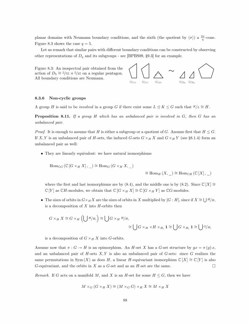
planar domains with Neumann boundary conditions, and the sixth (the quotient by 〈σ〉) a 2πq -cone.

Figure 8.3 shows the case q = 5.Let us remark that similar pairs with different boundary conditions can be constructed by observing

other representations of Dq and its subgroups - see [BPBS09, §9.3] for an example.

Figure 8.3: An isospectral pair obtained from theaction of D5

∼= Z/5Zo Z/2Z on a regular pentagon.All boundary conditions are Neumann.

8.3.6 Non-cyclic groups

A group H is said to be involved in a group G if there exist some L E K ≤ G such that K/L ∼= H.

Proposition 8.11. If a group H which has an unbalanced pair is involved in G, then G has anunbalanced pair.

Proof. It is enough to assume that H is either a subgroup or a quotient of G. Assume first that H ≤ G.If X,Y is an unbalanced pair of H-sets, the induced G-sets G×H X and G×H Y (see §8.1.4) form anunbalanced pair as well:

• They are linearly equivalent: we have natural isomorphisms

HomCG (C [G×H X] ,_) ∼= HomG (G×H X,_)

∼= HomH (X,_) ∼= HomCH (C [X] ,_)

where the first and last isomorphisms are by (8.4), and the middle one is by (8.2). Since C [X] ∼=C [Y ] as CH-modules, we obtain that C [G×H X] ∼= C [G×H Y ] as CG-modules.

• The sizes of orbits inG×HX are the sizes of orbits inX multiplied by [G : H], since ifX ∼=⋃H/Hi

is a decomposition of X into H-orbits then

G×H X ∼= G×H(⋃

H/Hi)∼=⋃G×H H/Hi

∼=⋃G×H ×H ×Hi 1 ∼=

⋃G×Hi 1 ∼=

⋃G/Hi

is a decomposition of G×H X into G-orbits.

Assume now that π : G H is an epimorphism. An H-set X has a G-set structure by gx = π (g)x,and an unbalanced pair of H-sets X,Y is also an unbalanced pair of G-sets: since G realizes thesame permutations in Sym (X) as does H, a linear H-equivariant isomorphism C [X] ∼= C [Y ] is alsoG-equivariant, and the orbits in X as a G-set and as an H-set are the same.

Remark. If G acts on a manifold M , and X is an H-set for some H ≤ G, then we have

M ×G (G×H X) ∼= (M ×G G)×H X ∼= M ×H X

88

i.e. the induced G-set gives the same manifold as does the original H-set.

Theorem 8.12. Every non-cyclic finite group has an unbalanced pair.

Proof. Let G be a non-cyclic finite group. Assume first that some p-Sylow group P ≤ G is not cyclic(in particular this is the case if G is abelian). Let Φ (P ) be the Frattini subgroup of P , which isthe intersection of all of its maximal proper subgroups. For any p-group P the quotient P/Φ(P ) isan elementary p-group of the same rank as P , so that if P is non-cyclic then P/Φ(P ) must containZ/pZ× Z/pZ. Therefore, Z/pZ× Z/pZ is involved in G and we are done by Proposition 8.11 and §8.3.2.

Zassenhaus classified the finite groups whose Sylow subgroups are all cyclic [Hal76, Thm. 9.4.3].They are of the form

Gm,n,r =⟨a, b∣∣ am = bn = e, b−1ab = ar

⟩= Z/mZoϑr Z/nZ

for m,n, r satisfying (m,n (r − 1)) = 1 (here ϑr (1) (1) = r, and rn ≡ 1 (modm) is implied to makeϑr : Z/nZ→ Aut (Z/mZ) ∼= (Z/mZ)

× a homomorphism). Since 0×kerϑr ≤ Z (G), and the quotient G/Z(G)

is never cyclic for nonabelian G, we can assume (by Proposition 8.11) that ϑr is injective. We canalso assume that n is prime, for otherwise for any nontrivial factor k of n we have a proper subgroup⟨a, bk

⟩= Z/mZ oϑ

rkZ/nk Z which is non-cyclic by the injectivity of ϑr. We can further assume that m

is prime. Otherwise, pick some prime q dividing m, and consider⟨am/q, b

⟩: it is cyclic only if ϑr fixes

am/q, i.e. arm/q = am/q, so that m | mq (r − 1), which is impossible since (m,n (r − 1)) = 1. Thus, by§8.3.4 we are done.

Since unbalanced G-sets are in particular non-isomorphic, this together with Proposition 8.10 givethe following:

Corollary 8.13. For a finite group G, the map Ω (G) → R (G) which takes a G-set X to the repre-sentation C [X] is injective iff G is cyclic.

Theorems 8.9 and 8.12 together imply the results announced in §1.6:

Corollary 8.14. If a finite non-cyclic group G acts faithfully by isometries on a compact connectedRiemannian manifold M , then there exist G-sets X,Y such that M ×GX and M ×G Y are isospectraland non-isometric.

From this follows:

Corollary 8.15. If M is a compact connected Riemannian manifold (or orbifold) such that π1 (M)

has a finite non-cyclic quotient, then M has isospectral non-isometric covers.

Proof. Let M be the universal cover ofM , and N a normal subgroup in π1 (M) such that G = π1(M)/N

is finite non-cyclic. M = M/N is a finite cover of M and thus compact, and G acts on it faithfully,with M/G = M . By the previous corollary there exist isospectral non-isometric unions of quotients ofM by subgroups of G, and these are covers of M .

89

8.4 Computation

Here we show how to compute, using GAP [GAP13], a basis for L (G), the ideal of linearly trivialelements in the Burnside ring Ω (G), which correspond to reduced pairs of linearly equivalent G-sets.We then consider an action of G and compute the isospectral pairs which correspond to this basis andaction.

Let G = D6 (see §8.3.5), and let Hi be a set of representatives for the conjugacy classes ofsubgroups of G (so that G/Hi is a Z-basis of Ω (G)). In the example which follows we compute thecorresponding quasiregular characters ci = SHi , which are the images of this basis under the mapΩ (G) → R (G). We then compute a basis for L (G), the kernel of this map, and apply the LLLalgorithm to this basis in order to possibly obtain a sparser one.

gap > G := DihedralGroup(12); ;

gap > H := List(ConjugacyClassesSubgroups(G), Representative); ;

gap > c := List(H, h −> List(PermutationCharacter(G, h))); ;

gap > LLLReducedBasis(NullspaceIntMat(c)).basis;

[[0, 1, 0,−1, 0, 0,−1, 0, 1, 0], [1,−1, 0,−1, 0, 0, 0,−1, 0, 2],

[−1, 1, 0, 1, 1, 0,−1, 0,−1, 0], [−1, 1, 1, 1, 0,−2, 0, 0, 0, 0]]

For example, the first element in the basis we obtained tells us that G/H2−G/H4−G/H7 +G/H9 vanishesin R (G), so that G/H2 ∪ G/H9 is linearly equivalent to G/H4 ∪ G/H7. One has to explore the outputof ConjugacyClassesSubgroups(G) to find out which subgroups these exactly are, or alternatively, toconstruct Hi oneself (in this case, for example, H2 belongs to the conjugacy class of 〈τ〉). The firstline in Table 8.1 presents representatives for the classes returned by ConjugacyClassesSubgroups(G),and the bottom four lines of the table show the basis that was calculated for L (D6) above. One maycheck that pairs II, III and IV are unbalanced.

Hi 〈1〉 〈τ〉⟨σ3⟩〈τσ〉

⟨σ2⟩〈τ,τσ3〉 〈τ,τσ2〉 〈σ〉 〈τσ,τσ3〉 〈τ,τσ〉

7/Hi

I 0 1 0 -1 0 0 -1 0 1 0

II 1 -1 0 -1 0 0 0 -1 0 2

III -1 1 0 1 1 0 -1 0 -1 0

VI -1 1 1 1 0 -2 0 0 0 0

Table 8.1: Representatives for the conjugacy classes of subgroups in D6, displayed with the corre-sponding quotients of the hexagon, and a basis for L (D6) = ker (Ω (D6)→ R (D6)).

Given an action of G on a manifold M , every difference of G-sets X − Y ∈ L (G) gives rise to anisospectral pair, namely M ×G X, M ×G Y . We consider the standard action of D6 on the regularhexagon, which we denote by 7. The second line in Table 8.1 shows the quotients 7/Hi correspondingto the subgroups Hi ≤ D6 in the topmost line, and we see that in this case there are no isometric

90

quotients arising from non-isomorphic G-sets. The isospectral pairs corresponding to the basis weobtained for L (D6) are shown in Table 8.2.

I ∼

II ∼

III ∼

IV ∼

I− III ∼

Table 8.2: The isospectral pairs corresponding to the basis for L (D6) described in Table 8.1, and anexample of an element obtained as a combination of these.

All isospectral pairs which arise from linear equivalences between D6-sets are spanned by thesefour, as explained in §8.2.3. The bottom line in Table 8.2 demonstrates such a pair (corresponding tothe element I− III). We remark that the pair corresponding to I is a hexagonal analogue of Chapman’s“two piece band” [Cha95] - such analogues exist for every n (but for odd n the isospectral pair obtainedis also isometric).

91

9 Generalizations and open questions

Isoperimetric constant

• As remarked after the statement of Theorem 1.2, one always has h (X) = 0 for X with a non-complete skeleton. One possible definition of a Cheeger constant for general complexes appearsin 5.5. Another natural candidate is the following:

h (X) = minV=

∐di=0 Ai

n · |F (A0, A1, . . . , Ad)||F ∂ (A0, A1, . . . , Ad)|

,

where F ∂ (A0, A1, . . . , Ad) denotes the set of (d− 1)-spheres (i.e. copies of the (d− 1)-skeletonof the d-simplex) having one vertex in each Ai. For a complex X with a complete skeleton,h (X) = h (X) as F ∂ (A0, . . . , Ad) = A0 × . . . × Ad. It is not hard to see that a lower Cheegerinequality does not hold here: consider any non-minimal triangulation of the (d− 1)-shpere, andattach a single d-simplex to one of the (d− 1)-cells on it. The obtained complex has λ = 0, andh = n. However, we conjecture that the upper bound still holds, namely, that the inequalityλ (X) ≤ h (X) holds for every d-complex.

• In Riemannian geometry, the Cheeger constant of a Riemannian manifold M is concerned withits partitions into two submanifolds along a common boundary of codimension one. The originalCheeger inequalities, due to Cheeger [Che70] and Buser [Bus82], relate the Cheeger constant tothe smallest eigenvalue of the Laplace-Beltrami operator on C∞ (M) = Ω0 (M). Can one definean isoperimetric quantity which concerns partitioning of M into d+ 1 parts, and relate it to thespectrum of the Laplace-Beltrami operator on Ωd−1 (M), the space of smooth (d− 1)-forms?

Random simplicial complexes

• In Lemma 5.6 it is shown that Linial-Meshulam complexes with expected degree O (log n) areexpanders. Is there a similar model for general complexes, for which the skeletons are notcomplete? Specifically, is there one in which the expected degrees of cells are only logarithmic inthe number of vertices - for example, a random triangle complex with n vertices, O(n log n) edges,and O(n log2 n) triangles, which is expanding (in contrast, we only know this for X

(2, n, C logn

n

)which has O

(n2 log n

)triangles).

• In the random graph model G = G (n, p) = X (1, n, p), taking p = kn with a fixed k gives

disconnected G a.a.s. However, random k-regular graphs are a.a.s. connected, and in fact areexcellent expanders (see e.g. [Fri08, Pud12]). In higher dimension, X = X

(d, n, kn

)has a.a.s.

a nontrivial (d− 1)-homology, and also h (X) = 0 (by Corollary 5.7 (2)). Can one constructa model for random regular complexes, and are these complexes high-dimensional expanders?This is interesting even for a weak notion of regularity, such as having a bounded fluctuation ofdegrees, or having all links of vertices isomorphic.

92

Random walk

• In an infinite connected graph, the limit of n√pvn (v) (which describes the spectral radius of the

transition operator, see §7.7) is independent of the starting point v. Is the same true in higherdimension? Namely, is lim supn→∞

n√Eσn (σ) independent of σ for a (d− 1)-connected complex?

• If X Y is a covering map of graphs, then λ (X) ≥ λ (Y ) (see e.g. [Kes59, Lemma 3.1], butbeware - Kesten uses λ (X) for what we denote by 1 − λ (X)). Does the same hold in higherdimension? If π : X Y is a covering map of d-complexes, then the same argumentation as ingraphs shows that for any σ ∈ Xd−1 and σ = π (σ) ∈ Y d−1 one has pσn (σ) ≤ pσn (σ) and alsopσn

(σ)≤ pσn (σ). This, however, does not suffice to show that E σn (σ) ≤ Eσn (σ). Showing that

this hold (or even that it holds after taking nth-roots and letting n→∞) would give the desiredresult.

• It is not hard to see that a (d+ 1)-partite d-complex is disorientable, but for d ≥ 2 one can alsoconstruct examples of disorientable complexes which are not (d+ 1)-partite. It seems reasonableto conjecture that for simply connected complexes these properties coincide. Is this indeed thecase?

• The suggestions for higher-dimensional analogues of amenability and transience raise severalquestions:

– Can high amenability and transience be characterized in non-spectral terms (i.e. combina-torial expansion, or some 1− 0 event in the (d− 1)-walk model)?

– Are the transience properties (T) and (T′) equivalent under some conditions?

– Are all d-complexes with degrees bounded by d+ 1 d-amenable?

• In classical settings, the Brownian motion on a Riemannian manifold constitutes a continuouslimit of the discrete random walk. Can one define a continuous process, say, on the (d− 1)-spherebundle of a Riemannian manifold, which relates to its (d− 1)-homology and to the spectrum ofthe Laplace-Beltrami operator on (d− 1)-forms?

• There are surprising and useful connections between random walks on graphs and electricalnetworks (see e.g. [DS84, LP05]). Can a parallel theory be devised for the random (d− 1)-walkon d-complexes?

Isospectrality

The isospectrality technique described in §8 (and thus Sunada’s technique as well) has actually littleto do with spectral geometry, since no property of the Laplace operator is used apart from being linearand commuting with isometries. For any linear operator F (on function spaces or other bundles, overmanifolds or general spaces), these methods produce F -isospectral objects, given an action of a groupwhich commutes with F .

However, it seems that in much more general settings, when a group action is studied, Sunada pairsare worth looking at. The most famous examples are Galois theory, giving Gassmann’s construction of

93

arithmetically equivalent number fields [Gas26], and Riemannian coverings, giving Sunada’s isospectralconstruction; but Sunada pairs were also studied in the context of Lie groups [DGL89], ergodic systems[LTW02], dessin d’enfants [MP10], the spectrum of discrete graphs [Bro96] and metric ones [SS06], theIhara zeta function of graphs [ST00], and the Witten zeta function of a Lie group [Lar04].

Sunada pairs in G correspond to linearly equivalent transitive G-sets, and we have seen that in thecontext of Riemannian coverings Sunada’s technique generalizes to non-transitive G-sets as well. It isnatural to ask whether other applications of Sunada pairs can be generalized in an analogous way. Ofparticular interest are unbalanced pairs, which do not exist in the transitive case (see Remark 8.8). Inthe settings of Riemannian manifolds they allowed us to deduce non-isometry, and one may hope thatthey play interesting roles in other situations.

94

References

[ABM05] R. Aharoni, E. Berger, and R. Meshulam, Eigenvalues and homology of flag complexes and vectorrepresentations of graphs, Geometric and functional analysis 15 (2005), no. 3, 555–566.

[AC88] N. Alon and F.R.K. Chung, Explicit construction of linear sized tolerant networks, Discrete Math-ematics 72 (1988), no. 1-3, 15–19.

[Alo86] N. Alon, Eigenvalues and expanders, Combinatorica 6 (1986), no. 2, 83–96.[AM85] N. Alon and V.D. Milman, λ1, isoperimetric inequalities for graphs, and superconcentrators, Jour-

nal of Combinatorial Theory, Series B 38 (1985), no. 1, 73–88.[Bal00] C.M. Ballantine, Ramanujan type buildings, Canadian Journal of Mathematics 52 (2000), no. 6,

1121–1148.[Bér92] P. Bérard, Transplantation et isospectralité I, Mathematische Annalen 292 (1992), no. 1, 547–559.[BKV+81] M. Blum, R.M. Karp, O. Vorneberger, C.H. Papadimitriou, and M. Yannakakis, Complexity of

testing whether a graph is a superconcentrator, Information Processing Letters 13 (1981), no. 4,164–167.

[BMS93] R. Beigel, G. Margulis, and D.A. Spielman, Fault diagnosis in a small constant number of par-allel testing rounds, Proceedings of the fifth annual ACM symposium on Parallel algorithms andarchitectures, ACM, 1993, pp. 21–29.

[Bor76] A. Borel, Admissible representations of a semi-simple group over a local field with vectors fixedunder an Iwahori subgroup, Inventiones mathematicae 35 (1976), no. 1, 233–259.

[BPBS09] R. Band, O. Parzanchevski, and G. Ben-Shach, The isospectral fruits of representation theory:quantum graphs and drums, Journal of Physics A: Mathematical and Theoretical 42 (2009), 175202.

[Bro96] R. Brooks, Some relations between graph theory and Riemann surfaces, Isr. Math. Conf. Proc. 11,Citeseer, 1996.

[Bus82] P. Buser, A note on the isoperimetric constant, Ann. Sci. École Norm. Sup.(4) 15 (1982), no. 2,213–230.

[Bus86] , Isospectral Riemann surfaces, Annales de l’Institut Fourier 36 (1986), no. 2, 167–192.[Cas80] W. Casselman, The unramified principal series of p-adic groups. I. The spherical function, Com-

positio Mathematica 40 (1980), no. 3, 387–406.[CDS94] P.B.J. Conway, P. Doyle, and K.D. Semmler, Some planar isospectral domains, Internat Math Res

Notices 9 (1994), 391–400.[Cha95] SJ Chapman, Drums that sound the same, American Mathematical Monthly 102 (1995), no. 2,

124–138.[Che70] J. Cheeger, A lower bound for the smallest eigenvalue of the Laplacian, Problems in analysis 195

(1970), 199.[CSŻ03] D.I. Cartwright, P. Solé, and A. Żuk, Ramanujan geometries of type An, Discrete mathematics

269 (2003), no. 1, 35–43.[DGL89] D.M. DeTurck, C.S. Gordon, and K.B. Lee, Isospectral deformations II: Trace formulas, metrics,

and potentials, Communications on Pure and Applied Mathematics 42 (1989), no. 8, 1067–1095.[DiP09] M. DiPasquale, On the order of a group containing nontrivial Gassmann equivalent subgroups,

Rose-Hulman Undergraduate Mathematics Journal 10 (2009), no. 1.[Dod84] J. Dodziuk, Difference equations, isoperimetric inequality and transience of certain random walks,

Trans. Amer. Math. Soc 284 (1984).[DR11] P.G. Doyle and J.P. Rossetti, Laplace-isospectral hyperbolic 2-orbifolds are representation-

equivalent, Arxiv preprint arXiv:1103.4372 (2011).[DS84] P.G. Doyle and J.L. Snell, Random walks and electric networks, no. 22, Mathematical Association

of America, 1984.[Eck44] B. Eckmann, Harmonische funktionen und randwertaufgaben in einem komplex, Commentarii

Mathematici Helvetici 17 (1944), no. 1, 240–255.

95

[ER59] P. Erdős and A. Rényi, On random graphs, Publicationes Mathematicae Debrecen 6 (1959), 290–297.

[Erd61] A. Erdos, P.and Rényi, On the evolution of random graphs, Bull. Inst. Internat. Statist 38 (1961),no. 4, 343–347.

[Fel66] W. Feller, An introduction to probability theory, vol. II, Wiley and Sons, New York, 1966.[FGL+12] J. Fox, M. Gromov, V. Lafforgue, A. Naor, and J. Pach, Overlap properties of geometric expanders,

J. Reine Angew. Math. 671 (2012), 49–83.[FP87] J. Friedman and N. Pippenger, Expanding graphs contain all small trees, Combinatorica 7 (1987),

no. 1, 71–76.[Fri98] J. Friedman, Computing Betti numbers via combinatorial Laplacians, Algorithmica 21 (1998),

no. 4, 331–346.[Fri08] , A proof of Alon’s second eigenvalue conjecture and related problems, Mem. Amer. Math.

Soc. 195 (2008), no. 910, viii+100. MR 2437174 (2010e:05181)[GAP13] The GAP Group, GAP – Groups, Algorithms, and Programming, Version 4.6.5, 2013.[Gar73] H. Garland, p-adic curvature and the cohomology of discrete subgroups of p-adic groups, The Annals

of Mathematics 97 (1973), no. 3, 375–423.[Gas26] F. Gassmann, Bemerkungen zur vorstehenden arbeit von Hurwitz, Math. Z 25 (1926), 124–143.[Gol13] K. Golubev, On the chromatic number of a simplicial complex, arXiv preprint arXiv:1306.4818

(2013).[GP13] K. Golubev and O. Parzanchevski, Spectrum and combinatorics of Ramanujan triangle complexes,

Preprint (2013).[Gro10] M. Gromov, Singularities, expanders and topology of maps. part 2: From combinatorics to topology

via algebraic isoperimetry, Geometric And Functional Analysis 20 (2010), no. 2, 416–526.[GW12] A. Gundert and U. Wagner, On Laplacians of random complexes, Proceedings of the 2012 sympo-

suim on Computational Geometry, ACM, 2012, pp. 151–160.[GWW92] C. Gordon, D.L. Webb, and S. Wolpert, One cannot hear the shape of a drum, American Mathe-

matical Society 27 (1992), no. 1.[GŻ99] R.I. Grigorchuk and A. Żuk, On the asymptotic spectrum of random walks on infinite families of

graphs, Random walks and discrete potential theory (Cortona, 1997), Sympos. Math 39 (1999),188–204.

[Hal76] M. Hall, The theory of groups, Chelsea Pub Co, 1976.[Hil08] L. Hillairet, Spectral decomposition of square-tiled surfaces, Mathematische Zeitschrift 260 (2008),

no. 2, 393–408.[HLW06] S. Hoory, N. Linial, and A. Wigderson, Expander graphs and their applications, Bulletin of the

American Mathematical Society 43 (2006), no. 4, 439–562.[Hof70] A.J. Hoffman, On eigenvalues and colorings of graphs, Graph theory and its applications (1970),

79–91.[Jan02] S. Janson, On concentration of probability, Contemporary combinatorics 10 (2002), no. 3, 1–9.[Kac66] M. Kac, Can one hear the shape of a drum?, The american mathematical monthly 73 (1966),

no. 4, 1–23.[Kes59] H. Kesten, Symmetric random walks on groups, Trans. Amer. Math. Soc. 92 (1959), 336–354. MR

0109367 (22 #253)[KLW10] M.H. Kang, W.C.W. Li, and C.J. Wang, The zeta functions of complexes from PGL(3): a

representation-theoretic approach, Israel Journal of Mathematics 177 (2010), no. 1, 335–348.[KRS00] W. Kook, V. Reiner, and D. Stanton, Combinatorial Laplacians of matroid complexes, Journal of

the American Mathematical Society 13 (2000), no. 1, 129–148.[Laf02] L. Lafforgue, Chtoucas de Drinfeld et correspondance de Langlands, Inventiones mathematicae 147

(2002), no. 1, 1–241.[Lar04] M. Larsen, Determining a semisimple group from its representation degrees, International Mathe-

matics Research Notices 2004 (2004), no. 38, 1989.

96

[Li04] W.C.W. Li, Ramanujan hypergraphs, Geometric and Functional Analysis 14 (2004), no. 2, 380–399.[LM06] N. Linial and R. Meshulam, Homological connectivity of random 2-complexes, Combinatorica 26

(2006), no. 4, 475–487.[LP05] R. Lyons and Y. Peres, Probability on trees and networks, Cambridge University Press, in prepa-

ration, 2005.[LPS88] A. Lubotzky, R. Phillips, and P. Sarnak, Ramanujan graphs, Combinatorica 8 (1988), no. 3, 261–

277.[LSV05a] A. Lubotzky, B. Samuels, and U. Vishne, Ramanujan complexes of type Ad, Israel Journal of

Mathematics 149 (2005), no. 1, 267–299.[LSV05b] , Explicit constructions of Ramanujan complexes of type Ad, Eur. J. Comb. 26 (2005), no. 6,

965–993.[LTW02] M. Lemańczyk, J.P. Thouvenot, and B. Weiss, Relative discrete spectrum and joinings, Monatshefte

für Mathematik 137 (2002), no. 1, 57–75.[Lub10] A. Lubotzky, Discrete groups, expanding graphs and invariant measures, vol. 125, Birkhauser,

2010.[Lub12a] , Expander graphs in pure and applied mathematics, Bull. Amer. Math. Soc 49 (2012),

113–162.[Lub12b] Alexander Lubotzky, Ramanujan complexes and high dimensional expanders, Takagi lectures 11

(2012), 29–58.[Lyo83] T. Lyons, A simple criterion for transience of a reversible Markov chain, The Annals of Probability

(1983), 393–402.[Mar88] G.A. Margulis, Explicit group-theoretical constructions of combinatorial schemes and their appli-

cation to the design of expanders and concentrators, Problemy Peredachi Informatsii 24 (1988),no. 1, 51–60.

[Mil64] J. Milnor, Eigenvalues of the Laplace operator on certain manifolds, Proceedings of the NationalAcademy of Sciences of the United States of America 51 (1964), no. 4, 542.

[MP10] M. Merling and R. Perlis, Gassmann equivalent dessins, Communications in Algebra 38 (2010),no. 6, 2129–2137.

[MS90] David W Matula and Farhad Shahrokhi, Sparsest cuts and bottlenecks in graphs, Discrete AppliedMathematics 27 (1990), no. 1, 113–123.

[MSS13] A. Marcus, D.A. Spielman, and N. Srivastava, Interlacing families I: Bipartite Ramanujan graphsof all degrees, arXiv preprint arXiv:1304.4132 (2013).

[MW11] J. Matoušek and U. Wagner, On Gromov’s method of selecting heavily covered points, Arxivpreprint arXiv:1102.3515 (2011).

[Nil91] A. Nilli, On the second eigenvalue of a graph, Discrete Mathematics 91 (1991), no. 2, 207–210.[Oli10] R.I. Oliveira, Concentration of the adjacency matrix and of the Laplacian in random graphs with

independent edges, Arxiv preprint ArXiv:0911.0600v2 (2010).[Pac98] J. Pach, A Tverberg-type result on multicolored simplices, Computational Geometry 10 (1998),

no. 2, 71–76.[Par13a] O. Parzanchevski, Mixing in high-dimensional expanders, arXiv preprint arXiv:1310.6477 (2013).[Par13b] , On G-sets and isospectrality, Annales de l’Institut Fourier, To appear (2013),

arXiv:1104.0315.[PB10] O. Parzanchevski and R. Band, Linear representations and isospectrality with boundary conditions,

Journal of Geometric Analysis 20 (2010), no. 2, 439–471.[PP14a] O. Parzanchevski and D. Puder, Stallings graphs, algebraic extensions and primitive elements

in F2, Mathematical Proceedings of the Cambridge Philosophical Society, To appear (2014+),arXiv:1210.6574.

[PP14b] D. Puder and O. Parzanchevski, Measure preserving words are primitive, Journal of the AmericanMathematical Society, To appear (2014+), arXiv:1202.3269.

[PR12] O. Parzanchevski and R. Rosenthal, Simplicial complexes: spectrum, homology and random walks,

97

arXiv preprint arXiv:1211.6775 (2012).[PRT14] O. Parzanchevski, R. Rosenthal, and R.J. Tessler, Isoperimetric inequalities in simplicial com-

plexes, Combinatorica, To appear (2014+), arXiv:1207.0638.[PS13] O. Parzanchevski and G. Schul, On the Fourier expansion of word maps, Bulletin of the London

Mathematical Society (2013), doi:10.1112/blms/bdt068.[Pud12] D. Puder, Expansion of random graphs: New proofs, new results, arXiv preprint arXiv:1212.5216

(2012).[Ser77] J.P. Serre, Linear representations of finite groups, vol. 42, Springer Verlag, 1977.[Ser80] , Trees, translated from french by John Stillwell, Springer Verlag, 1980.[SS06] T. Shapira and U. Smilansky, Quantum graphs which sound the same, Non-linear dynamics and

fundamental interactions (2006), 17–29.[ST00] H.M. Stark and A.A. Terras, Zeta functions of finite graphs and coverings, part II, Advances in

Mathematics 154 (2000), no. 1, 132–195.[ST11] D.A. Spielman and S.H. Teng, Spectral sparsification of graphs, SIAM Journal on Computing 40

(2011), no. 4, 981–1025.[Sun85] T. Sunada, Riemannian coverings and isospectral manifolds, The Annals of Mathematics 121

(1985), no. 1, 169–186.[Tad86] M. Tadic, Classification of unitary representations in irreducible representations of general lin-

ear group (non-archimedean case), Annales scientifiques de l’Ecole normale supérieure, vol. 19,Elsevier, 1986, pp. 335–382.

[Tan84] R.M. Tanner, Explicit concentrators from generalized n-gons, SIAM Journal on Algebraic andDiscrete Methods 5 (1984), 287.

[Zel80] A.V. Zelevinsky, Induced representations of reductive p-adic groups II. On irreducible representa-tions of GL(n), Annales Scientifiques de l’École Normale Supérieure, vol. 13, Société mathématiquede France, 1980, pp. 165–210.

[Żuk96] A. Żuk, La propriété (T) de Kazhdan pour les groupes agissant sur les polyedres, Comptes rendusde l’Académie des sciences. Série 1, Mathématique 323 (1996), no. 5, 453–458.

98