NBER WORKING PAPER SERIES

HIGH FREQUENCY EVIDENCE ON THE DEMAND FOR GASOLINE

Laurence LevinMatthew S. LewisFrank A. Wolak

Working Paper 22345http://www.nber.org/papers/w22345

NATIONAL BUREAU OF ECONOMIC RESEARCH1050 Massachusetts Avenue

Cambridge, MA 02138June 2016

The views expressed herein are those of the authors and do not necessarily reflect the views of the National Bureau of Economic Research.

NBER working papers are circulated for discussion and comment purposes. They have not been peer-reviewed or been subject to the review by the NBER Board of Directors that accompanies official NBER publications.

© 2016 by Laurence Levin, Matthew S. Lewis, and Frank A. Wolak. All rights reserved. Short sections of text, not to exceed two paragraphs, may be quoted without explicit permission provided that full credit, including © notice, is given to the source.

High Frequency Evidence on the Demand for GasolineLaurence Levin, Matthew S. Lewis, and Frank A. WolakNBER Working Paper No. 22345June 2016JEL No. L91

ABSTRACT

Daily city-level expenditures and prices are used to estimate the price responsiveness of gasoline demand in the U.S. Using a frequency of purchase model that explicitly acknowledges the distinction between gasoline demand and gasoline expenditures, we consistently find the price elasticity of demand to be an order of magnitude larger than estimates from recent studies using more aggregated data. We demonstrate directly that higher levels of spatial and temporal aggregation generate increasingly inelastic demand estimates, and then perform a decomposition to examine the relative importance of several different sources of bias likely to arise in more aggregated studies.

Laurence LevinVISA Decision Sciences901 Metro Center BoulevardMail Stop: M3-2BFoster City , CA 94404-2775llevin@visa.com

Matthew S. LewisJohn E. Walker Department of Economics Clemson University 228 Sirrine Hall Box 341309 Clemson, SC 29634-1309mslewis@clemson.edu

Frank A. WolakDepartment of EconomicsStanford UniversityStanford, CA 94305-6072and NBERwolak@zia.stanford.edu

1 Introduction

The price elasticity of demand for gasoline has been extensively studied over the last 40

years, and for good reason. Understanding gasoline demand responsiveness is critical in

determining gasoline tax rates and evaluating alternative policies that target the negative

externalities associated with automobile use (pollution, road congestion, etc.). In the U.S.,

continuing pressure to address climate change has prompted a variety of policy proposals at

the national level as well as legislative action at the state level. Starting in 2015, California

extended its cap-and-trade program for greenhouse gas emissions to cover transportation

fuels, and a number of other states have significantly increased their gasoline tax rates.

Gasoline prices have also become increasingly volatile as a result of periodic shortages in

available refining capacity and increased uncertainty in world oil markets. Understanding

consumers’ ability to respond to such price fluctuations is crucial for predicting the potential

macroeconomic impacts of future petroleum supply disruptions and for evaluating the ben-

efits of policy measures intended to mitigate these effects, such as the maintenance and use

of the U.S. Strategic Petroleum Reserve or the use of temporary gasoline tax suspensions.

While empirical studies of gasoline demand have adopted a variety of different es-

timation strategies, nearly all of them face the challenge of having to work with imperfect

and often highly aggregated data.1 Many utilize monthly, quarterly, or even annual ag-

gregate proxies of gasoline usage and average prices, often from a single national time

series.2 Others rely on cross-sectional data in an attempt to identify demand elasticities

based on price variation across regions or countries. In reality, individuals make gasoline

consumption decisions on a daily basis, responding directly to the gasoline prices observed

in their local area on that day. Empirical models relating monthly or annual gasoline vol-

umes to average prices across broad geographic areas necessarily aggregate these different

consumption decisions and are likely to mask a significant share of the response by con-1There are a number of survey articles and meta-analyses available (including Dahl and Sterner, 1991;

Goodwin, 1992; Espey, 1998; Basso and Oum, 2007; Brons et al., 2008) that summarize and analyze theliterature on gasoline demand estimation.

2The most commonly used proxy for gasoline consumption from the U.S. Energy Information Administrationmeasures the volume of gasoline disappearing from refineries or pipelines minus the estimated volume ofgasoline exported.

1

sumers a local price change. Moreover, the use of highly aggregated data generally requires

strong assumptions that restrict the demand relationship from varying across locations or

over time. As a result, unobserved heterogeneity in underlying demand has the potential

to bias elasticity estimates. Perhaps not surprisingly given such challenges, these aggregate

studies have produced a wide range of different estimates of demand elasticity. Academic

and government studies evaluating potential policy interventions in gasoline markets fre-

quently rely on estimates from this literature or adopt the same problematic methods to

obtain estimates despite the fact that the elasticity values can often substantially impact

predicted policy outcomes.

Our study uses daily gasoline prices and citywide gasoline expenditures from 243

U.S. cities to analyze the impact of daily prices on daily gasoline demand. These high-

frequency panel data have several important advantages. First, the expenditure informa-

tion comes from credit card transactions at the point of sale and, therefore, offers a much

more direct measure of consumer purchases. Second, observing sales and prices daily at

the city-level allows us to model demand at the level that purchase decisions actually occur,

rather than by relating average consumption across cities over some time-period to a cor-

responding average price. Finally, our panel data can be exploited by including extensive

fixed effects to better control for persistent differences in gasoline demand over time and

across locations.

Our approach yields robust estimates of the elasticity of consumers’ demand for

gasoline by utilizing a more accurate point-of-sale measure of consumption and adopting

an empirical strategy that leverages the higher frequency and greater geographic detail of

our consumption and price data to avoid the biases potentially impacting the estimates and

policy conclusions of previous studies. Second, we derive a decomposition identifying the

different sources of bias that arise in more aggregate models and then examine the relative

magnitudes of these different biases by estimating demand models at varying levels of data

aggregation. The results of the decomposition help to clarify why the different empirical

approaches utilized in the literature tend to generate such different estimates of the demand

elasticity.

2

Unlike the existing literature our analysis also directly addresses the fundamental

difference between gasoline demand (or usage) and gasoline expenditures—a difference

that becomes even more pronounced when using daily data. The price of gasoline on a

particular day can influence both how much gasoline a consumer uses in that day as well as

whether they decide to make a gasoline purchase. Our approach more accurately models

the demand for gasoline in a manner that recognizes the distinction between expenditure

and consumption. We specify a two-equation model of the consumer’s probability of gaso-

line purchase and daily gasoline demand that separates the demand decision from the pur-

chase decision in the most flexible manner possible given our city-level expenditure data.

Because we observe both the number of gasoline transactions and the total expenditures on

gasoline, we are able to separately identify changes in consumers’ probability of purchase

from changes in consumers’ underlying demand for gasoline. Aggregating our two-equation

model of individual gasoline purchase and demand over all individuals in a metropolitan

area yields a model of daily aggregate gasoline expenditures that we can use to recover a

price elasticity of demand for the metropolitan area.

Using this model we obtain estimates of gasoline demand elasticity ranging from

−.27 to −.35. These responses are nearly an order of magnitude more elastic than some

recent (and commonly cited) estimates from comparable studies (Hughes, Knittel and Sper-

ling, 2008; Small and Van Dender, 2007; Park and Zhao, 2010), implying that changes in

gasoline prices or taxes may have a much larger impact on gasoline usage or greenhouse

gas emissions than one might otherwise predict. Recent events seem to reflect this sub-

stantial responsiveness in gasoline demand. Declining gas prices during 2015 and 2016

have reportedly resulted in dramatic reductions in public transit ridership, increases in ve-

hicle miles traveled, and surge in sales of vehicles with lower fuel economy (Morath, 2016;

Sommer, 2015). While studies using aggregate data from the 1970’s and 80’s commonly

reported gasoline demand elasticity estimates around −.25 to −.303, our aggregation re-

sults suggest that many of these estimates were also likely to have been biased and that

actual demand response in earlier decades may have been substantially more elastic than3Surveys of these earlier results include: Dahl and Sterner (1991); Goodwin (1992); Espey (1998); Basso

and Oum (2007)

3

previously thought.

Like other studies using similar static models of gasoline demand, our estimates

should be interpreted to reflect the short-run demand response that occurs over a period

of several months or years, rather than the longer-run demand responses that could occur

over decades (potentially capturing expansions in public transit or the development of more

efficient cars). However, our daily data also allow us to also investigate whether demand

or consumer purchase decisions respond differently in the very short run. We consider

a dynamic two-equation frequency of purchase model which incorporates lagged prices,

allowing the immediate response of demand to a price change to differ from the longer

run demand response. We find evidence that gasoline expenditures respond even more

strongly in the days immediately following a price change (mainly due to a response in

the probability of purchase), but this temporary additional response largely dissipates after

4 to 5 days. The response that remains is nearly identical to that estimated by our main

(static) analysis. This further supports the argument that the estimates from our baseline

static model accurately reflect the same type of longer-run response that previous studies

attempt to estimate using monthly or annual data, rather than the very-short run response

that occurs in the days immediately following the shock.

In the second part of our analysis we investigate the consequences of estimating

demand using more highly aggregated data as is common in previous studies. As a first

step, we use our data to estimate a standard demand model aggregated over time and

across cities to varying degrees. The resulting estimates become increasingly less elastic as

the level of data aggregation increases. Estimating the model using our data aggregated to a

national time-series of monthly total expenditures and average prices results in elasticities

that are indistinguishable from zero, suggesting that studies using aggregated data may

substantially underestimate consumers’ price responsiveness.

Next, to better understand the impacts of data aggregation, we derive a decompo-

sition identifying three distinct components of bias that arise in more aggregate demand

models. First, demand models that assume a common price coefficient are often estimated

even though the underlying coefficients have the potential to differ across cities. While the

4

coefficient obtained from this restricted model does estimate a weighted average of these

coefficients, the weighting applied to each individual coefficient will generally change when

the model is estimated at a more spatially and temporally aggregated level. A second possi-

ble source of bias arises from correlation between the aggregated prices and the aggregated

day-of-sample and city fixed effects that appear in the disaggregated model. While this

bias will not occur in panel data models that retain a complete set of two-way fixed effects,

many of the studies in the existing literature estimating time-series or cross-sectional mod-

els or panel models with incomplete fixed effects may be subject to this form of bias. The

final source of potential bias arises when correlation between the average prices and error

term is created as a result of aggregation. The typical OLS identification assumptions for

a disaggregate demand model would require the price in a given city on a given day to be

uncorrelated with the unobserved demand shock in that city on that day. However, correla-

tion between prices and demand shocks on other days or in other cities can cause the prices

and errors in the aggregated panel data to be correlated, resulting in biased estimates.

Comparing our daily city-level estimates with those obtained using aggregated data

we are able to estimate the magnitude of the bias resulting from each of these three compo-

nents. The results reveal how the primary source of bias differs depending on the dimension

and degree of aggregation. Observed biases are largest in time series models where time-

period fixed effects can no longer be used to control for demand differences over time.

The sources of bias identified in our decomposition and the magnitudes suggested

in our aggregated regressions help to provide a more systematic explanation of why stud-

ies using different methodologies have obtained different elasticity estimates. Consistent

with our findings, recent time-series studies including Hughes et al. (2008) and Park and

Zhao (2010) tend to produce very inelastic estimates, potentially caused by significant pos-

itive bias. Studies estimating panel regressions (though at a more aggregated level than

ours) including Davis and Kilian (2011) and Li et al. (2014) are not subject to the most

significant source of bias and report more elastic estimates. However, these panel estimates

are still lower than those obtained in our daily city-level regressions. Our decomposition

provides guidance to researchers in evaluating whether particular market environments or

data sources may be more susceptible to the forms of correlation that are likely to result in

5

bias when estimating demand models using aggregate data, and is sufficiently general that

it can be used to evaluate almost any form of aggregation.

Accurate estimates of gasoline demand elasticity are crucial to making effective pub-

lic policy decisions. As we discuss in Section 7, the stronger demand response revealed in

our analysis suggests that carbon tax and fuel tax policies may have a substantially larger

impact on fuel use and greenhouse gas emissions than might be concluded based on other

recent studies. Similarly, the predicted impact on gasoline prices resulting from a supply

restriction such as a refinery or pipeline outage or even from the implementation of an

emissions cap-and-trade policy is likely to be significantly smaller than might otherwise

be expected. Our findings help clarify the need to be cautious when in utilizing elastic-

ity estimates based on aggregate data and highlight how the availability of more detailed

information could substantially improve policy analysis.

2 Approaches to Estimating Gasoline Demand

2.1 Common Estimation Strategies

There are a number of survey articles available (including Dahl and Sterner, 1991; Good-

win, 1992; Espey, 1998; Basso and Oum, 2007) that summarize and analyze the literature

on gasoline demand estimation. Nevertheless, it is helpful to provide a brief overview of

some of the benefits and limitations of a number of commonly used empirical approaches

in order to motivate our analysis and highlight the contribution of our study.

Most studies of aggregate gasoline demand estimate a simple log-linear model of

quantity as a function of the gasoline price and other variables such as average income to

control for shifts in demand. This specification is chosen mostly for convenience, so that the

coefficient on price represents an estimate of demand elasticity. A number of studies have

investigated alternative functional forms, and some find alternative forms to have a better

fit (e.g., Hsing, 1990), but generally the resulting elasticity estimates are not substantially

impacted by specification (see Sterner and Dahl, 1992; Espey, 1998).

Such “static” demand models can be appropriate as long as the researcher believes

6

that the price and quantity data in the sample represent observations from a stable rela-

tionship. In situations where it is thought that gasoline demand may take multiple peri-

ods to adjust to price changes, researchers often include a lagged dependent variable (the

parsimonious partial adjustment model approach) or specify a distributed lag model (the

more flexible approach) in which lagged values of prices and other control variables are

also included in the demand equation. Coefficients on lagged prices capture how demand

temporarily deviates from the longer-run equilibrium relationship as adjustment occurs, al-

lowing the sum of the coefficients on current and lagged prices to more accurately capture

the overall elasticity of demand in the longer run.

2.2 Identification

Regardless of functional form, demand specifications are most typically estimated using

OLS. As a result, if sufficient controls cannot be included in the demand equation, endo-

geneity of the price variable can arise as a result of supply side responses to unobserved

demand shifts. The instrumental variables approaches often adopted in other contexts are

rarely used in studies of gasoline demand due to a lack of credible instruments. Time-series

studies and even some panel-data studies rely almost exclusively on macroeconomic con-

trol variables, like average income, and seasonal dummy variables (when relevant), which

are certainly jointly determined with aggregate gasoline demand but do not perfectly pre-

dict fluctuations in gasoline usage. In this case, it is reasonable to expect this endogeneity

bias to make price elasticity estimates more inelastic than they should be. Higher levels of

data aggregation tend to exacerbate this problem, making it difficult to include sufficient

control variables and still have enough variation left in the data to identify demand. Our

identification strategy leverages the availability of high-frequency panel data to include ex-

tensive sets of time and cross-sectional fixed effects in order to eliminate potential sources

of endogeneity.

Two main factors determine the severity of bias that will result from price endo-

geneity in OLS estimates of demand: the prevalence and magnitude of unobserved demand

shocks relative to unobserved supply shocks and the elasticity of the supply curve. If de-

mand shifts are relatively small or the relevant supply curve is fairly flat, then observed

7

variation in price will mainly be the result of upward and downward shifts in the supply

curve. Correspondingly, our empirical specifications attempt to include fixed effects that

will remove most of the unobserved variation in demand while leaving a sufficient level of

supply variation to accurately identify the demand elasticity. Moreover, given the nature of

the gasoline storage and distribution infrastructure, the daily supply of gasoline is likely to

respond very elastically to any remaining daily demand shocks that are not absorbed by the

included fixed effects.4

Most of the variation in daily city-level gasoline demand is likely to come from

persistent differences across cities in per-capita gasoline consumption and from economic

changes that influence gasoline demand over time nationwide. These demand shifts repre-

sent the primary sources of potential endogeneity, and so our baseline demand specification

controls for these by including both city and day-of-sample fixed effects. The fixed effects

also remove a significant amount of supply variation including that generated by fluctua-

tions crude oil prices over time or by persistent regional differences in costs, competition,

environmental restrictions, or gasoline tax levels. However, temporary regional gasoline

supply shocks resulting from refinery outages or pipeline disruptions or regional variation

in seasonal gasoline content restrictions can create significant variation in the relative price

levels across cities that will not be absorbed by fixed effects. Our identification of demand

relies largely on these periodic shifts in local supply. While it is possible that demand shifts

remain even with city and day-of-sample fixed effects included in the model, these will

mostly come from predictable seasonal patterns or day-of-week purchase patterns which

can be adequately planned for through adjustments to inventories, refinery production, or

pipeline delivery schedules. Any additional idiosyncratic day-to-day fluctuations in local

purchasing are likely small enough to be easily accommodated using local terminal in-

ventories, so that relative price fluctuations not absorbed by city and day-of-sample fixed

effects should entirely reflect localized supply-side cost shocks. In other words, within the4Based on average inventory levels and daily consumption, there is typically enough gasoline stored at local

distribution terminals and refineries to supply 4 weeks worth of demand (for more information see the U.S.Energy Information Administration’s Petroleum Supply Monthly). In addition, gas stations often have severaldays of inventory in their underground tanks. Day-to-day fluctuations in demand can easily be supplied from acombination of these sources, allowing intertemporal arbitrage that minimizes the likelihood of any substantialprice response.

8

context of our model, the relevant daily supply curve is likely to be almost perfectly elastic,

minimizing any potential for endogeneity bias in our OLS estimates. For robustness, how-

ever, we are also able to estimate alternative specifications that include city-specific sets of

month-of-year and day-of-week fixed effects to control for potential differences across cities

in seasonal or weekly demand patterns yet still preserve the supply variation resulting from

unexpected refinery or pipeline disruptions.

While studies using aggregate data generally must resort to controlling for demand

shocks with observable controls and/or a more limited set of fixed effects, several recent

papers have attempted identify and utilize instrumental variables to more accurately model

demand. Hughes et al. (2008) estimate a specification of nationwide monthly gasoline de-

mand using crude oil production disruptions as instruments for monthly gasoline prices, but

find the resulting elasticity estimates to be nearly indistinguishable from those obtained in

their baseline OLS specifications. Davis and Kilian (2011) utilize monthly state-level aggre-

gate gasoline consumption and average prices to estimate a first-differenced model in which

changes in state gasoline tax rates serve as instrumental variables for changes in gasoline

price. Their preferred IV estimate suggests a demand elasticity of −0.46 (s.e. = 0.23), while

the corresponding OLS monthly state-level panel regression produces a substantially less

elastic estimate of −0.19 (s.e. = 0.04) and an estimation using data aggregated to the na-

tional monthly time series level produces an even smaller elasticity of −0.09 (s.e. = 0.04).5

Davis and Kilian’s IV estimate is much closer to our disaggregated elasticity estimates, sug-

gesting that both their IV approach and our disaggregated panel fixed effects approach may

be overcoming the potential simultaneity bias caused by baseline demand differences over

time.6 While we don’t observe enough state tax changes during our sample to consider such

an instrument, as another robustness check we do estimate an IV specification (described in

Appendix C) using regional wholesale spot gasoline prices as an instrument for local retail5Coglianese, Davis, Kilian and Stock (2015) point out that the IV estimate of Davis and Kilian (2011) may

be biased as a result of consumers anticipating the tax change and buying more gas in the month before the taxincrease than in the month after. When one month leads and lags are included to control for this, the elasticityestimate falls to −0.36 (s.e. = 0.24), nearly identical to the estimate we obtain from our frequency of purchasemodel.

6An important caveat is that their measure differs from ours in that it focuses on the demand responseoccurring during the month in which the corresponding state gasoline tax rate change occurs, which is likely toreflect a shorter run elasticity than is captured in our baseline model.

9

prices and obtain results similar to our OLS regressions.

3 Retail Gasoline Price and Expenditure Data

Our data contains daily gasoline price and expenditure data for 243 metropolitan areas

throughout the United States from February 1, 2006 to December 31, 2009. For each city

average daily retail prices of unleaded regular gasoline are obtained from the American

Automobile Association’s (AAA) Daily Fuel Gauge Report. The prices reported by AAA

are provided by the Oil Price Information Service (OPIS) which constructs the city average

prices using station-level prices collected from fleet credit card transactions and direct feeds

from gas stations.7

Our expenditure data were obtained from the financial services company Visa Inc.

The data reflect the total dollar amount of purchases by all Visa debit and credit card users

at gas stations within a city on a given day. As with the price data, cities are defined

based on the geographic definition of the associated Metropolitan Statistical Area (MSA).

In addition to total citywide expenditures, the Visa data also include the number of gasoline

transactions or purchases taking place at gas stations in each city during each day. This

allows us to separate the daily probability of purchase from the daily demand for gasoline.

We also observe the total number of Visa cards that are actively purchasing (any product)

within the current month. We use this as a measure of the total population of cards at risk

of recording a gasoline purchase during each day of that month.8

Although the data has many advantages, Visa does not directly observe the price

paid at the pump or the quantity of gasoline purchased by the customer. Instead, we con-

struct a measure of the total quantity of gasoline purchased in a particular MSA on a par-

ticular day by dividing the total expenditures of Visa card customers at gas stations by the7The OPIS price survey is the most comprehensive in the industry and is commonly used in research on

gasoline pricing.8At two points during the sample period (August 1, 2006 and August 1, 2007) Visa made small adjustments

to their merchant classification methodology which produce discrete jumps in our measure of gas station ex-penditures in some cities. To correct for this we estimate all models with additional city-specific data-periodfixed effects allowing the average expenditures and transaction counts to differ before, between, and after thesetwo dates.

10

average regular unleaded gasoline price in the city on that day. This approximation raises

several potential issues which we explore and address below.

First, in dividing total gas station expenditures by the regular gasoline price we are

ignoring the fact that around 15% of gas purchases are for mid-grade or premium gasoline

which sell at higher prices. If the fraction of regular-grade purchases were fairly constant

over time, we would not expect this unobserved price difference to impact our demand

elasticity estimates. However, the results of Hastings and Shapiro (2013) suggest that some

consumers may substitute from premium to regular grade gasoline when prices increase. In

Appendix A we discuss this possibility in more detail, derive an expression for the potential

bias, and use the estimates of Hastings and Shapiro (2013) to show that any such bias is

very likely to be negligible in our context.

A second and potentially more important source of bias arises from the fact that to-

tal gas station expenditures are also likely to include some non-gasoline purchases. Simply

dividing total expenditure by the gasoline price to produce a measure of quantity ignores

this possibility. If non-gasoline purchases are present, expenditures will appear more elastic

to gasoline price changes. Even if the prices and demand for non-gasoline items are not

correlated with the price of gasoline, dividing these expenditures by the price of gasoline

will mechanically generate an elasticity of −1 for the non-gasoline portion of the trans-

action.9 In general, the share of revenues generated by non-gasoline items is small but

non-trivial. According to the 2007 U.S. Economic Census, gasoline stations in the U.S. re-

ceive just over 21% of their total revenues from non-fuel sales.10 Fortunately, biases from

non-fuel purchases are only a concern for in-store transactions, and our data includes the

daily city-level expenditures and number of transactions separately for pay-at-pump and in-

store purchases. Pay-at-pump purchases represent over 76% of total expenditures and over

64% of all transactions in our data.11 Estimating gasoline demand using only pay-at-pump9See Appendix B for a more complete discussion of the resulting bias.

10Most of these non-fuel revenues come from food, cigarettes, and alcohol. Fuel sales often generate lessthan half of a station’s profits, but given the high volume sold it still represents the vast majority of stationrevenues.

11On average pay-at-pump transactions are larger (in dollar value) than in-store transactions. The most likelyexplanation is that some in-store transactions include only non-fuel items which tend to be less expensive thanthe typical gasoline purchase. Unfortunately, our data do not allow us to examine the distribution of individualtransaction amounts since we only observe the total expenditure for the day in each city.

11

transactions gives an alternative estimate of elasticity that is not subject to this bias and may

give some indication of the magnitude of the bias for in-store transactions. In addition, in

Appendix B we derive the magnitude of the bias that would be expected when non-gasoline

expenditures are present in the data, and use outside estimates of non-gasoline expendi-

tures to construct bias-corrected elasticity estimates. The results are consistent with the

notion that estimating elasticities using pay-at-pump purchases fully eliminates (or perhaps

even over-compensates for) any bias resulting from non-gasoline expenditures.

In the interest of completeness our analysis will present estimates utilizing all pur-

chases as well as estimates using only pay-at-pump purchases. To be conservative however,

we will mostly use pay-at-pump purchase data in our alternative specifications and supple-

mentary analysis.

3.1 Descriptive Statistics

Before we begin our empirical analysis it is helpful to highlight some important features

of the data. First, the price data reveal significant idiosyncratic fluctuation across cities.

Though prices in all cities are impacted by common factors like world oil prices, there are

many other factors that influence prices locally. Persistent price differences across states

arise as a result of differences in gasoline tax rates or in the blends of gasoline that are

required. More importantly, significant transitory differences in daily prices across the MSAs

arise frequently during our sample period. Figure 1 compares retail price fluctuations in Los

Angeles, Chicago, and New York over a typical 100 day period in 2007. It is clear that daily

city-level prices provide much richer price variation than monthly data with which to study

demand response.

Daily gasoline expenditures also follow different patterns across MSAs, presumably

due to both independent retail price movements and other city-specific events. Note that

daily expenditures necessarily change with retail prices because they represent the total

quantity purchased multiplied by the price paid. As noted earlier, we create a measure of the

total quantity of gasoline purchased each day using total daily expenditures divided by the

daily average retail price for each MSA . Figure 2 presents a normalized seven-day moving

12

Figure 1: Daily Average Retail Gasoline Prices for Selected Cities

2.80

3.00

3.20

3.40

8/22/07 9/11/07 10/1/07 10/21/07 11/10/07 11/30/07

Retail Price − Los Angeles, CA Retail Price − Chicago, IL Retail Price − New York, NY

Figure 2: Seven Day Moving Average of Total Quantity Purchased for Selected Cities Nor-malized by the City Average

0.90

0.95

1.00

1.05

1.10

1.15

8/22/07 9/11/07 10/1/07 10/21/07 11/10/07 11/30/07

Los Angeles, CA Chicago, IL New York, NY 7−day Moving Average of Normalized Quantity Purchased

13

average of this measure of the daily quantity purchased for the same three cities depicted

in Figure 1 over the same period.12 The daily quantities for each MSA are normalized by

the average quantity purchased in that MSA over the sample period. Just as with the prices,

the quantities move together at times but also exhibit significant differences. As an example

of the type of variation that will be important for our empirical identification of demand,

note that as the daily average price in California increases from being the lowest to the

highest of the three cities by the end of the time period in Figure 1, the normalized quantity

demanded falls from being the highest to the lowest over the same time period in Figure 2.

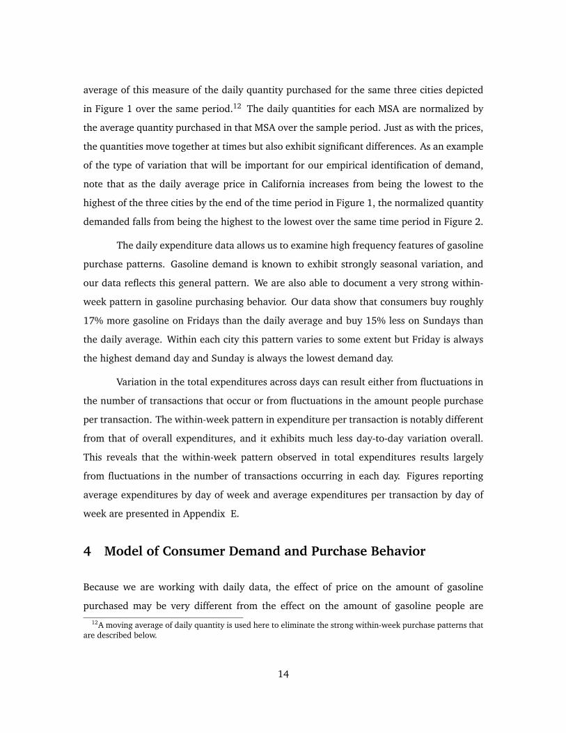
The daily expenditure data allows us to examine high frequency features of gasoline

purchase patterns. Gasoline demand is known to exhibit strongly seasonal variation, and

our data reflects this general pattern. We are also able to document a very strong within-

week pattern in gasoline purchasing behavior. Our data show that consumers buy roughly

17% more gasoline on Fridays than the daily average and buy 15% less on Sundays than

the daily average. Within each city this pattern varies to some extent but Friday is always

the highest demand day and Sunday is always the lowest demand day.

Variation in the total expenditures across days can result either from fluctuations in

the number of transactions that occur or from fluctuations in the amount people purchase

per transaction. The within-week pattern in expenditure per transaction is notably different

from that of overall expenditures, and it exhibits much less day-to-day variation overall.

This reveals that the within-week pattern observed in total expenditures results largely

from fluctuations in the number of transactions occurring in each day. Figures reporting

average expenditures by day of week and average expenditures per transaction by day of

week are presented in Appendix E.

4 Model of Consumer Demand and Purchase Behavior

Because we are working with daily data, the effect of price on the amount of gasoline

purchased may be very different from the effect on the amount of gasoline people are12A moving average of daily quantity is used here to eliminate the strong within-week purchase patterns that

are described below.

14

actually demanding at any given time. Consumers can buy and store gasoline in their car,

which implies that a consumer’s daily demand for gasoline can differ from its expenditures

on gasoline. This section presents a theoretical model that recovers an estimate of the

daily price elasticity of the unobserved demand for gasoline from data on the daily number

of purchases and expenditures on gasoline for each MSA. A latent customer-level daily

demand for gasoline and daily purchase probability give rise to an econometric model for

customer-level daily gasoline expenditures that we then aggregate to the MSA level.

Suppose the daily demand for each customer in a city j on a day d takes the form:

djd = exp(αj + λd + βln(pjd) + εjd), (1)

where αj is a fixed-effect for MSA j, λd is the fixed-effect for day-of-sample d, pjd is the price

of gasoline for day d in region j, and β is the price elasticity of demand. For each j, the εjd

are a sequence of unobserved mean-zero random variables that may be heteroscedastic and

correlated over time within each MSA but are distributed independently across MSAs and

are independent of pjd. Consumers must periodically purchase gasoline to satisfy this level

of daily usage. The probability that a consumer in MSA j purchases gasoline on a day d is

assumed to equal:

ρjd = γj + δd. (2)

where γj is a fixed-effect for MSA j and δd is the day-of-sample fixed effect for day d. We

assume that the expenditure on gasoline during day d by each customer in MSA j, ejd, is

related to the consumer’s daily purchase probability and daily gasoline demand through the

following relationship:

ejd =pjddjdρjd

. (3)

This model implies that the actual quantity of gasoline purchased (if purchase occurs) times

the daily probability of purchase is equal to the daily quantity demanded by that customer.

Because our data is at the MSA level we aggregate the customer-level model of daily gaso-

line expenditures over the total number of customers in MSA j during day d, Njd. The

number of customers in MSA j during day d making a gasoline purchase is equal to njd.

15

Therefore, Ejd, total gasoline expenditures during day d for MSA j can be expressed as:

Ejd = ejdnjd =pjdd(pjd, εjd)njd

ρjd. (4)

Because we observe the total number of active Visa cards (Njd) in MSA j during day

d, and the total number of gasoline transactions (njd), njd/Njd is an unbiased estimate of

ρjd, the probability of purchase for MSA j during day d. Accordingly, we can estimate the

parameters of equation 2 using OLS applied to:

njdNjd

= γj + δd + νjd, (5)

where the νjd are a sequence of mean-zero random variables that may be heteroscedastic

and correlated with εjd and over time within each MSA but are distributed independently

across MSAs. We can use the fitted values ρ̂jd = γ̂j + δ̂d to obtain a consistent estimates

of the ρjd. Substituting the estimated purchase probability into Equation 4 and taking logs

generates our econometric model of gasoline expenditures:

ln(Ejd) = αj + λd + (β + 1)ln(pjd) + ln(njd)− ln(ρ̂jd) + εjd. (6)

This model can alternatively be expressed in terms of the quantity purchased:

ln(Qjd) = αj + λd + βln(pjd) + ln(njd)− ln(ρ̂jd) + εjd, (7)

The empirical model in Equation 7 makes it possible to identify the underlying MSA-

level elasticity of demand for gasoline (β) using data on prices, the quantity purchased, and

the number of transactions. In Equations 1 & 2 the demand and probability of purchase are

both assumed to vary by city and day of sample, but different combinations of fixed effects

can easily be used to generate alternative specifications for each of these functions. We will

also consider a specification that includes both lagged and current prices in the demand

and purchase probability equations.

5 Estimation and Results

5.1 Frequency of Purchase Model

We begin by estimating city-level demand for gasoline using the model expressed in Equa-

tion 7. Results are reported in Table 1. Following the discussion of data concerns in Sec-

16

Table 1: Estimates of Baseline Empirical Model of Demand

Dependent Variable = ln(quantityjd)Pay-at-Pump Only All Purchases

(1) (2) (3) (4) (5) (6)ln(pricejd) −0.295 −0.364 −0.301 −0.378 −0.465 −0.408

(0.031) (0.022) (0.006) (0.030) (0.022) (0.008)ln(# of transactionsjd) 1 0.996 1 1.021

(0.002) (0.004)ln(predicted probability −1 −0.003 −1 0.006

of purchasejd) (0.001) (0.002)Note: Day-of-sample fixed effects and city fixed effects are included in all specifications. Standard errors in

Columns 1 & 4 are robust and clustered to allow serial correlation within city. Standard errors for the remaining

specifications are generated using a nonparametric bootstrap that allows errors to be serially correlated within

a city and jointly distributed with the error term in the first-stage regression.

tion 3, our main specifications are estimated using pay-at-pump purchases only, but we

also report the results when all purchases are used. The model implies that coefficients

on ln(njd) and ln(ρ̂jd) should be 1 and −1 respectively. We estimate the model with this

restriction imposed and without it. To facilitate comparisons with earlier studies of gasoline

demand we also include (in Columns 1 & 4) estimates from a basic log-linear aggregate

demand model. For the basic model we report heterskedacticity consistent standard error

estimates that allow for arbitrary serial correlation within each city. Standard error esti-

mates for the purchase model are generated using a nonparametric bootstrap to account

for the fact that the predicted probability of purchase is estimated in a first-stage regres-

sion.13

When estimated using pay-at-pump transactions only, the model with all restrictions

yields an elasticity estimate of −.36, while the unrestricted model produces a similar elas-

ticity estimate of −.30. The unrestricted coefficient on ln(njd) is very close to 1, but the

13Given that there are C cities and D days in the sample, the procedure first re-samples with replacement Cpairs of OLS residual vectors of length D from the purchase probability equation and the expenditure equationfor the same city. These are combined with the OLS estimates of the fitted values for both equations to computere-sampled purchase frequencies and expenditure levels vectors of length DC. The two-step estimation pro-cedure is then repeated for the resampled purchase frequency equation and then for the expenditure equationwith the logarithm of the fitted value from the estimated purchase frequency equation used as a regressor in theexpenditure equation to obtain estimates for the parameter values for both equations for that re-sample. Thesample variance of these re-samples is then used to compute the estimated standard errors for both parametervectors.

17

coefficient on ln(ρ̂jd) is very close to zero; far from the −1 implied by the theory. This

may be because the fixed effects absorb most of the variation in the probability of purchase

(given the functional form specified in Equation 7), and any variation left may be measured

with error. The estimated price elasticity is still similar to that from the model with restric-

tions imposed. Estimates of both the restricted and unrestricted models are somewhat more

elastic when using data from all purchases as would be expected if the inclusion of in-store

purchases results in some bias from non-gasoline transactions. Nevertheless, the pattern of

estimates across specifications is similar for the pay-at-pump and all-transaction samples.

The coefficient estimates from the basic demand model in Columns 1 & 4 are quite close to

those generated by our frequency of purchase model.

Including time fixed effects helps to control for shifts in demand, but it can also mask

supply shifts that could help to better identify demand elasticity. Hence, as an alternative

specification we estimate the demand model using month-of-sample fixed effects rather

than day-of-sample. Day-of-week fixed effects are also included to control for the weekly

pattern in demand suggested by Figure 3. The resulting coefficient estimates, reported in

Table 2, Column 1, are very similar to those of the benchmark pay-at-pump specification,

with the price elasticity estimated to be −.28, suggesting that month-of-sample and day-of-

sample fixed effects appear to work similarly in controlling for macroeconomic or gasoline

market specific fluctuations that might impact gasoline demand at the national level.

In all the specifications estimated to this point, demand elasticities are identified

off of city-specific variation in price and quantity purchased. However, large city-specific

or regional demand shifts occurring over time have the potential to bias these elasticity

estimates. Therefore, we estimate an additional set of specifications that include additional

controls for city-specific demand patterns. Table 2, Column 2 reports the results of a regres-

sion including month-of-sample effects for each city as well as day-of-week fixed effects.

Column 3 contains the estimates from a model including a full set of national day-of-sample

fixed effects in addition to the city-specific month-of-year effects to allow seasonal patterns

in demand to differ across cities. Column 4 adds further flexibility by including both day-

of-sample and city-specific month-of-sample fixed effects. The estimated elasticities vary

somewhat across these models, but are all of a similar magnitude to the baseline estimates

18

Table 2: Estimates from Alternative Specifications

Dependent Variable = ln(quantityjd)Pay-at-Pump Transactions

(1) (2) (3) (4)ln(pricejd) −0.278 −0.271 −0.301 −0.351

(0.011) (0.012) (0.006) (0.005)ln(# of transactionsjd) 1.007 1.010 0.989 0.994

(0.006) (0.006) (0.002) (0.002)ln(predicted probability 0.009 0.011 −0.003 −0.002

of purchasejd) (0.006) (0.006) (0.001) (0.001)

Fixed Effects:Day of Week X XMonth of Sample XDay of Sample X XCity XMonth of Year × City XMonth of Sample × City X X

Note: Standard errors are generated using a nonparametric bootstrap that allows

errors to be arbitrary serial correlated within a city and jointly distributed with the

error term in the first-stage regression.

in Table 1. It is important to note, however, that once separate month-of-sample fixed ef-

fects are included for each city they absorb any deviations from the national average that

last longer than one month. As a result, the elasticity estimate in Column 4 only reflects the

response in demand that occurs in the 4 weeks following a change in price. This estimate is

slightly more elastic than in the other specifications suggesting that very short run demand

response is even more elastic than that which persists over a longer time horizon.14 In gen-

eral, however, the results reveal that relatively elastic estimates of demand can be obtained

using a variety of different sources of variation within the data and are not sensitive to a

particular functional form.

Though the ability to include extensive fixed effects should minimize any poten-

tial endogeneity bias that might result from unobserved demand shocks, it is difficult to

conclude with certainty that these demand shocks have been entirely eliminated. Unob-14This result is confirmed when we explore the differences in longer-run vs shorter-run demand response in

more detail in Section 5.2.

19

served city-specific demand shocks could still bias our elasticity estimates downward if lo-

cal distribution terminals are not able to plan ahead or use inventories to costlessly absorb

these differences (i.e., if the local supply curve is not highly elastic with respect to daily

adjustments). As a final robustness check, we have estimated an instrumental variables

specification that utilizes spot market (wholesale) gasoline prices from large regional re-

fining centers (New York Harbor, the Gulf Coast, or Los Angeles) as instruments for local

retail prices. Market-wide fluctuations in wholesale gasoline prices resulting from a com-

bination of changes in demand and changes in crude oil and refining costs are captured

by day-of-sample fixed effects, but differences in wholesale gasoline prices between regions

still exhibit significant variation largely driven by unexpected refinery shocks. Under the

assumption that this regional variation in spot prices is relatively unaffected by temporary

city-specific demand fluctuations, using this IV approach could help to eliminate any re-

maining endogeneity generated by correlation between city-level prices and local demand

shocks.

The results of these IV specifications (described in more detail and reported in Ap-

pendix C) largely confirm that the robustness of the main OLS findings. The IV estimates of

both the basic aggregate demand model and the frequency of purchase model are slightly

more elastic but of a relatively similar magnitude to those reported in Tables 1 & 2.

What is most striking about these findings, in general, is that the elasticity estimates

from both our frequency of purchase model and the basic log-linear aggregate demand

model are consistently several times more elastic than those from comparable recent studies

including Hughes et al. (2008) whose estimates range from −.034 to −.077 for the period

2000–2006 and Park and Zhao (2010) whose time-varying estimates ranges from around

−.05 in 2000 to around −.15 in 2008. Our daily city-level purchase data clearly reveal a

much greater degree of demand response than has been suggested by much of the literature.

It is important to highlight that the use of daily data rather than, say, monthly

data does not imply that our elasticity estimates describe a “shorter run” demand response.

The relevant response horizon of any elasticity estimate depends on the variation in prices

used to identify the response parameter and when these movements occur relative to when

20

demand is observed. Prices change in this market on a daily basis and consumers make

purchase decisions on a daily basis, so behavior is likely to be more accurately represented

using a model of daily demand for gasoline. However, as in most studies, our baseline model

is static and does not allow the degree of demand responsiveness to change depending on

how long it has been since a price change occurred, so price changes occurring several

months ago are just as important as price changes occurring days or weeks ago in terms of

identifying demand elasticity.15 As a result, we believe that our main elasticity estimates

reflect the same type of consumer response that other studies attempt to measure using

more aggregated monthly or quarterly data. In the next section, we leverage our daily data

by relaxing these assumptions in the model to investigate if demand responds differently in

the very short run.

5.2 Short Run vs Longer Run Demand Elasticity

To this point our models have assumed that prices influence gasoline demand entirely

through the current gasoline price, implying that all demand response occurs immediately.

In practice, however, it is not unusual for the demand curves to be more elastic in the

short run than in the long run. Perhaps the most common of these situations occurs when

consumers can hold inventories and in the short run choose to add to or withdraw from

inventories in response to price changes even when they do not significantly change their

consumption in the long run. Gasoline consumers obviously hold small inventories of gaso-

line in their vehicle’s tank, so this behavior is feasible on a limited scale. Similarly, con-

sumers may have the ability to postpone (or expedite) some necessary trips or utilize public

transportation in response to a temporary increase (or decrease) in price, regardless of how

they change their overall driving habits. These types of behavior imply that, for a given

gasoline price today, the amount of gasoline purchased today might depend on whether the

price has been at or near its current level for a while or whether it was significantly higher

or lower a few days or a few weeks ago.

The elasticity estimate from most gasoline demand models (including our baseline15Specifically, our model of daily demand implies that if the daily price rose by 10 percent and remained

at this higher level, daily gasoline demand would remain lower by an amount equal to 10 percent times ourdemand elasticity for as long as the daily price remained 10 percent higher.

21

model) represent some average of these shorter-run and longer-run responses. However,

with daily data it is possible to separately identify these different responses by allowing

demand to depend on past prices as well as current price levels. Moreover, by using the

structure of our consumer purchase model and including past prices along with current

prices in both the individual demand and purchase equations, we are able to decompose

any potential short-run responses to examine whether consumers appear to be significantly

altering gasoline usage or simply shifting when they make purchases in the days following a

price change. If consumers are substituting away from driving in response to price increases

then their daily demand may be influenced by past prices. If consumers are using their

inventories of gasoline strategically, both current and past prices may influence a consumer’s

probability of purchase. We alter Equations 1 & 2 to allow for these types of behavior. The

demand for each customer in a city j on a day d can be specified as:

djd = exp(αj + λd + βln(pjd) +∑l∈L

ζlln(pj,d−l) + εjd), (8)

where pj,d−l represents the price l days prior to the current period and L represents the set

of lags lengths included in the specification. Similarly, the probability of purchase can be

expressed as:

ρjd = γj + δd + ψln(pjd) +∑l∈L

ηlln(pj,d−l). (9)

Leaving the consumer purchase model from Section 3 otherwise unchanged results in the

following final representation of the aggregate quantity purchased in city j on day d:

ln(Qjd) = αj + λd + βln(pjd) +∑l∈L

ζlln(pj,d−l) + ln(njd)− ln(ρ̂jd) + εjd, (10)

where the predicted purchase probability can be estimated from an OLS regression of:

njdNjd

= γj + δd + ψln(pjd) +∑l∈L

ηlln(pj,d−l) + νjd. (11)

In both the demand equation and the purchase probability equation we include log

of the current price and the lagged log prices from each of the previous 5 days as well as

longer lags of 10 and 20 days. Lags longer than 20 days are omitted as their inclusion

22

Table 3: Purchase Model with Lagged Prices

Traditional Model Purchase Frequency ModelDemand Purchase DemandEquation Equation Equation

(1) (2) (3)ln(pricejd) −0.775 −0.009 −0.458

(0.081) (0.002) (0.009)ln(pricej,d−1) −0.607 −0.028 0.098

(0.098) (0.002) (0.008)ln(pricej,d−2) 0.637 0.023 −0.002

(0.091) (0.001) (0.007)ln(pricej,d−3) 0.393 0.014 0.052

(0.044) (0.001) (0.006)ln(pricej,d−4) 0.184 0.003 0.020

(0.046) (0.002) (0.007)ln(pricej,d−5) 0.055 0.003 −0.011

(0.039) (0.002) (0.007)ln(pricej,d−10) −0.076 −0.003 0.0002

(0.021) (0.001) (0.003)ln(pricej,d−20) −0.119 −0.001 0.004

(0.021) (0.001) (0.004)ln(# of transactionsjd) 0.995

(0.002)ln(predicted probability −0.003

of purchasejd) (0.001)

Total Implied Elasticity −0.308 0.061 −0.29620 Days After a Price Change

Note: City and day of sample fixed effects are present in all specifications. The dependent variable in

Column 1 is the log of the average quantity purchased at the pump per capita by Visa customers in city

j on day d. Standard errors in Column 1 are robust and clustered to allow arbitrary serial correlation

within a city. The dependent variables Columns 2 & 3 are the share of Visa customers purchasing at

the pump and the log of the quantity purchased at the pump by Visa customers in city j on day d.

Standard errors in Columns 2 & 3 are generated using a nonparametric bootstrap that allows errors to

be arbitrary serial correlated within a city and jointly distributed with the error term in the first-stage

regression.

23

requires the use of a shorter sample for estimation, but when price lags of 40 and 60 days

are included their coefficients are small in magnitude and do not substantially affect the

estimates of the existing coefficients. For comparison we also estimate a similar version

of the more traditional single-equation demand specification that includes lagged prices.

Coefficient estimate from the traditional model are reported in in Column 1 of Table 3

and estimates from the demand and purchase probability equations from the frequency of

purchase model are reported in Columns 2 & 3. All specifications are estimated using only

pay-at-pump purchases. The final row of the table includes the total implied elasticity of

the probability of purchase or of demand response after 20 days.16 Estimates from the

traditional demand model and the demand equation in the purchase model are directly

comparable to the corresponding specifications without lags in of Table 1.

In the traditional demand model (Column 1), the coefficients on the current and

previous day’s log price are negative and much larger in magnitude than the corresponding

elasticity estimated without lags. The sum of the first two coefficient estimates in Column 1

imply that the amount of gasoline purchased one day after a 1% price increase will will

be 1.38% lower than it would have been without the price increase. During the following

3 to 4 days, however, the amount purchased tends to increase sharply, back towards its

original level, canceling out much of the very strong initial response in purchasing. The 10-

and 20-day lags reveal that the price response becomes slightly stronger once again, several

weeks after the price change. Adding together the coefficients of all the price lags in the

regression gives the response of demand 20 days after a permanent price change. This sum

of coefficients is reported in the last row of Table 3 and implies that the elasticity of demand

response after 20 days is −.31, nearly identical to the elasticities of −.30 identified in our

baseline model with no lags.

Coefficient estimates from the frequency of purchase model in columns (2) and (3)

of Table 3 reveal that the large response in the amount of gasoline purchased in the days

following a price change results almost entirely from a temporary change in the probability

of making a purchase rather than a change in gasoline demand or usage. The probability

16For the demand equations this is simply the sum of all the log-price coefficients. For the probability ofpurchase equation this is the sum of all the log-price coefficients divided by the mean probability of purchase.

24

of purchase falls (rises) significantly on the day of and particularly on the day following a

price increase (decrease). The coefficients on ln(pj,d) and ln(pj,d−1) imply that the purchase

probability one day after a price change exhibits an elasticity with respect to price of around

−1.12 all else equal.17 However, this response in the probability of purchase in the day of

and the day after a price change is entirely counteracted over the following few days to

leave the elasticity of the overall response of purchase probability after 20 days to be small

and slightly positive at .06.

In the demand equation (Column 3) the inclusion of lagged prices causes the coef-

ficient on the current value of ln(pjd) to increase in magnitude, suggesting an even larger

immediate demand response to price changes. As in the basic demand specification of Col-

umn 1, however, the sum of the coefficients on the current and lagged values of ln(pjd)

in the demand equation are very similar to the coefficient estimates for ln(pjd) when no

lagged prices are included (Table 1, Column 3). In other words, the total demand response

to a price shock that lasts longer than a few days exhibits a demand elasticity of around

−.30, nearly identical to the estimates in our baseline purchase model. The results also

reveal a small additional response within the first few days of a price shock, consistent with

the idea that consumers delay/expedite gasoline usage by a few days in response to price

fluctuations, but this effect does not appear to be as large as those resulting from changes

in the probability of purchase.

The results of both the traditional demand model and the purchase frequency model

provide evidence of a stronger responsiveness to price changes in the very short run, but

also confirm that these responses occur in addition to a more persistent response which

very closely resembles that implied by our earlier specifications. We conclude from this that

previous studies utilizing monthly or annual data did not obtain lower elasticity estimates

a result of consumers being less responsive to price changes that persist over longer time

periods. Instead, as we show in the next section, the use of such temporally aggregated

data is likely to bias elasticity estimates causing demand to appear less responsive than can

be revealed when using daily data.17The average probability of purchase by a cardholder on a give day is 0.033, so the elasticity of the probability

of purchase is computed as (−.009 −.028)/.033 = −1.12.

25

6 Examining the Divergence from Previous Findings

Given the rather large discrepancy between our elasticity estimates and those found in other

recent studies, we discuss in this section a number of differences in our analyses that could

potentially explain this disparity.

6.1 Sources of Gasoline Consumption Data

Perhaps the biggest challenge in studying gasoline demand is finding an accurate measure

of consumption. Nearly all available measures are recorded at a highly aggregated level

and are likely to measure actual gasoline usage within the specified time interval with a

considerable amount of error. The most common source used in recent time series or panel

studies (e.g., Hughes et al., 2008; Park and Zhao, 2010; Lin and Prince, 2013) is the U.S.

Energy Information Administration’s (EIA’s) data on finished motor gasoline “product sup-

plied”. These data are constructed from surveys of refineries, import/export terminals, and

pipeline operators, and the volumes reported reflect the disappearance of refined product

from these primary suppliers into the secondary distribution system (local distributers and

storage facilities). Each month the EIA reports amounts disappearing as the product sup-

plied in each of the nation’s five Petroleum Area Defense Districts (PADDs). Unfortunately,

given distribution lags and storage capabilities, the amount of product flowing from sec-

ondary distributors to retailers and ultimately to consumers could differ substantially from

the amount received by these suppliers in any given time period. In addition, to generate

a measure that represents domestic gasoline usage, the EIA must net out from total pro-

duction the estimated quantity of gasoline exported for use in other countries. This step

provides yet another dimension for potential error, and created serious measurement issues

in 2011 during a period of rapidly growing refined product exports.18

Another potential data source for gasoline consumption is the Federal Highway Ad-

ministration (FHWA), which collects information from each state on the number of gallons

of motor gasoline for which state excise taxes have been collected each month. This mea-

sure would appear to be more closely linked to consumption and it is available at the state18See Cui (2012).

26

level rather than the PADD level. However, a significant amount of measurement error is

generated by the fact that each state has its own procedures and systems for collecting this

information. The point in the supply chain at which the fuel is taxed also varies across

states. Some require taxes to be paid when the distributer first receives the fuel, while

others tax the volume of gasoline sold by the distributor. In fact, the FHWA includes in its

publications the disclaimer that the reported volumes “may reflect time lags of 6 weeks or

more between wholesale and retail levels.”19

In contrast to the EIA and FHWA data, our measure of gasoline expenditures from

Visa is recorded at the final step of the distribution process—when the consumer purchases

the product from the retailer. This eliminates the possibility that changes in consumer pur-

chase volumes are masked by additions or withdrawals from local storage. Moreover, it

allows daily city-specific volumes to be observed and more accurately linked with contem-

poraneous local prices, providing for a more direct identification of demand response.

6.2 Estimating Demand Elasticity Using Aggregated Data

In general, using highly aggregated data can mask much of the temporal and geographic

co-movements in prices and quantities that result from consumer demand response and

also make it more difficult to empirically identify consistent estimates of such response. To

illustrate this point, suppose the per-capita daily demand for gasoline in MSA c during day

d can be represented as:

qcd = Dcd(pcd, Xcd) + εcd, (12)

where pcd is price of gasoline in region c on day d and Xcd is the vector of characteristics of

region c and day d that enter the demand function for that region and day. These daily de-

mand functions for each MSA imply that Qm, the national average daily per-capita demand

for gasoline during month m, is equal to the sum of total consumption (qcdNcd) across cities

and days divided by the sum of the total population (Ncd) across cities and days:

Qm =

∑d ∈ Am

∑Cc=1NcdDcd(pcd, Xcd)∑

d ∈ Am

∑Cc=1Ncd

+

∑d ∈ Am

∑Cc=1Ncdεcd∑

d ∈ Am

∑Cc=1Ncd

, (13)

19FHWA Highway Statistics 2010, Table MF-33GA, Footnote 1.

27

where C is the total number of MSAs in the sample and Am denotes the set of days in

month m. This aggregation process implies that the national monthly demand for gasoline

depends on the daily prices for all days during that month for all MSAs, rather than simply

a single monthly national average price. Similarly, a monthly state-level average demand

would depend on the daily prices for all days during that month for all MSAs in that state.

However, this is not the model estimated in most empirical studies of aggregate demand.

Typically these studies only have access to aggregated price measures as well, and, as a

result estimate something like:

Qm = D̃(pm, X̃m) + ε̃m where pm =1

Am

1

C

∑d ∈ Am

C∑c=1

pcd. (14)

Given the data generating process in (12), the model in (14) will only hold under

very specific assumptions, such as the case in which the Dcd(pcd, Xcd) function is linear and

identical across cities and each εcd is uncorrelated not just with pcd and Xcd but also with

the values of these variables in other cities and periods over which aggregation occurs.20

If these conditions are not collectively satisfied in the markets being examined, then biases

arising from aggregation have the potential to explain the large differences observed be-

tween our elasticity estimates and those from previous studies. Fortunately, we are able to

investigate the impact of aggregation by using our data to create new data sets with varying

levels of temporal and geographic aggregation. We construct daily data sets of state level

and nationwide total quantity purchased and average price, as well as three monthly data

sets at the city, state, and national levels. To facilitate a more direct comparison with other

studies, we estimate basic log-log aggregate demand models and use aggregate per-capita

quantities calculated as the corresponding sum of the daily quantity purchased divided by

the total number of Visa customers in the combined area. For consistency, average prices

are also computed as a per-capita weighted average across cities and days.

As in our main analysis, a complete set of time period and cross-sectional fixed ef-

fects are used whenever possible to control for shifts in demand. When using daily national

time series data we include day-of-week and month-of-sample fixed effects. For the monthly

national time series we are restricted to using month of year (i.e. seasonal) fixed effects, so20The various issues necessities such strong assumptions will be detailed in Section 6.3.

28

per capita real personal disposable income is included as an additional control for demand

shifts.21 This final specification is identical to that of Hughes et al. (2008).

The demand estimates for each level of aggregation appear in Panel A of Table 4.

The top rows report the results when estimated using pay-at-pump purchases only while

the bottom rows report the results for all purchases. The first column reports the daily

city-level results again for comparison. The next three columns contain panel regressions

with varying levels of temporal and/or geographic aggregation. Price elasticity estimates

from these specifications are all very similar to each other (between −.22 and −.25 for

pay-at-pump purchases and between −.30 and −.34 for all purchases) and are less elastic

than corresponding estimates from the disaggregated regression in Column 1. The elasticity

estimates from the two time series regressions in Columns 5 & 6 are even smaller in magni-

tude, being indistinguishable from zero for pay-at-pump purchases and ranging from −.12

to −.14 for all purchases; much closer to the elasticities reported by Hughes et al. (2008)

in their national time-series study.22 Clearly, increasing levels of aggregation lead to less

elastic estimates of demand, particularly when moving from panel to time series data.

6.3 Sources of Aggregation Bias

In this section we decompose the impact of using different forms of aggregate price and

quantity data on the resulting elasticity estimates. Rather than assess the impact of aggre-

gating data with a log-log demand specification and have to deal with the fact that the sum

across days or cities of the log price or quantity is not the same as the log of the sum, we

consider a linear demand specification that can be aggregated using linear operations. To

evaluate the importance of this functional form choice, we begin by estimating estimating

these linear demand models at different levels of aggregation, just as was done with the

log-log model. In Panel B of Table 4, we report both coefficient estimates and the implied

elasticities evaluated at mean values of quantity per capita, price, and income per capita.

Although the linear and log-log specifications have the potential to yield different results,21Data on per capita personal disposable income comes from the Bureau of Economic Analysis.22In Appendix D we replicate the exact model of Hughes et al. (2008) using their data source but from

our 2006–2009 time period and show the results to be very similar to our pay-at-pump national time-seriesestimates.

29

Table 4: Regressions Using Aggregated Data

Geography: city city state state national nationalPeriodicity: daily monthly daily monthly daily monthly

(1) (2) (3) (4) (5) (6)Panel A: Log-Log Model: Dependent Variable = ln(quantity per capita)Pay-at-Pump Only:

ln(priceit) −0.323 −0.246 −0.245 −0.215 −0.014 −0.002(0.025) (0.028) (0.059) (0.066) (0.067) (0.021)

ln(incomeit) 0.339(0.171)

All Purchases:ln(priceit) −0.405 −0.338 −0.325 −0.295 −0.137 −0.130

(0.024) (0.028) (0.065) (0.073) (0.064) (0.016)ln(incomeit) 0.458

(0.146)Panel B: Linear Model: Dependent Variable = quantity per capitaPay-at-Pump Only:

priceit −0.046 −0.037 −0.030 −0.025 −0.009 −0.003(0.004) (0.004) (0.009) (0.010) (0.008) (0.002)

incomeit 0.005(0.002)

Implied Elasticities:price −0.312 −0.247 −0.201 −0.164 −0.062 −0.008income 0.379

All Purchases:priceit −0.077 −0.064 −0.058 −0.050 −0.035 −0.026

(0.006) (0.007) (0.016) (0.018) (0.009) (0.003)incomeit 0.010

(0.002)Implied Elasticities:price −0.379 −0.313 −0.285 −0.245 −0.174 −0.128income 0.613

Fixed Effects:Day of Sample X XDay of Week XMonth of Sample X X XMonth of Year XCity X XState X X

Note: Standard errors for panel specifications are robust and clustered at the level of the cross-

sectional unit to allow for arbitrary serial correlation. Standard errors for time-series specifications

are estimated using the Newey-West (1987) procedure and are robust to the forms of serial correla-

tion they consider. Implied elasticities are calculated at the sample-wide mean values of quantity per

capita, price, and income.30

for our data, the levels of the elasticity estimates evaluated at the sample mean of the data

and the degree to which they change across increasing levels of aggregation are quite sim-

ilar. We conclude from this comparison that the differences in estimates resulting from

data aggregation apparent in our setting is relatively pervasive and is not the result of a

particular functional form assumption or a particular mode of aggregation.

6.3.1 Decomposing the Impact of Aggregation on Elasticities in a Linear Model

Most studies of gasoline demand focus on a model in which all locations are assumed to

have the same price coefficient, our decomposition analysis considers a more general data

generating process in which the daily city-level per-capita demand for gasoline depends

linearly on the price of gasoline with a slope that may differ across cities:

Qcd = αd + λc + βcpcd + εcd, (15)

where c=1,...,C, d=1,...,D, C = 241 is the number of cities, and D = 1430 is the number of

days in our sample. This model can be written in matrix notation as:

Q = (IC ⊗ ιD)α + (ιC ⊗ ID)λ + Pβ + ε, (16)

where Q = (Q′1,Q′2, ...,Q

′C)′, Qc = (Qc1,Qc2, ...,QcD)′, ιC is a C × 1 vector on 1’s, ιD

is a D × 1 vector on 1’s, IC is a C × C identity matrix, ID is a D ×D identity matrix, α is

a C × 1 vector of city fixed effects, and λ is a D × 1 vector of day-of-sample fixed effects.

To account for the fact that each city can potentially have a different slope coefficient, P is

a CD × C matrix with the cth column having zeros everywhere but the cth block of length

D which is replaced with the D × 1 vector pc = (pc1, pc2, ..., pcD)′, β = (β1, β2, ..., βC)

′

and ε = (ε′1, ε′2, ..., ε

′C)′, εc = (εc1, εc2, ..., εcD)

′. Let Z = [IC ⊗ ιD | ιC ⊗ ID] equal the

DC × (D + C) matrix and δ = (α′, λ′)′ a (D + C) × 1 vector. In terms of this notation

(16) becomes:

Q = Zδ + Pβ + ε. (17)

Equation 17 can be estimated directly using OLS to recover an estimate of each

city’s βc. However, it is more common for a more restricted model of gasoline demand to be

31

estimated in which all locations are assumed to have the same price coefficient, implying

the following true model:

Q = Zδ∗ + (PιC)β∗ + ε∗. (18)

PιC is a DC × 1 vector that equals p = (p′1,p′2, ...,p

′C)′ and β∗ is a scalar.

Applying OLS to (17) yields:

Q = Zd + Pb + e, (19)

where d,b, and e are the OLS estimates of δ, β, and ε, respectively. Pre-multiplying both

sides of (19) by MZ = IDC − Z(Z′Z)−1Z′ yields

MZQ = MZPb+ e, (20)

where b = (P′MZP)−1P′MZQ. In terms of this notation, the OLS estimate of β∗ is

b∗ = (ιC′P′MZPιC)

−1ι′CP′MZQ. Substituting the expression for Q from (19) and rec-

ognizing that MZZ = 0 and MZe = e yields

b∗ = (ιC′P′MZPιC)

−1ι′CP′MZPb = (p′MZp)

−1p′MZPb, (21)

Note that if (16) is the true data generation process, then the OLS estimate b∗ is a weighted

average of the OLS estimates of βc in which the relative weighting of each city’s βc is based

on the degree of within-city variation in the residual prices (after controlling for city and

day-of-sample fixed effects). As we demonstrate below, different data aggregations will

yield different weighted sums of the OLS estimates of the βc as a component of the estimated

slope coefficient.

Using this notation, we can also derive expressions for the OLS estimate of the slope

coefficient with different quantity and price aggregates in terms of d,b, and e . Consider a

regression model aggregated to the month and state level. Suppose their are S states and

M months. This can be accomplished by pre-multiplying Q and p by a SM ×DC matrix A.

Assume that the rows of this matrix are ordered in blocks by states and within each block

by months and the columns of the matrix are ordered in blocks by cities and then by days

within each block. The mth row of the sth block is composed zeros for all elements except

32

those where city c is contained in state s and day d is contained in month m. In those cases

the element of the matrix is equal to Ncd the number of active purchasers in city c in day

d divided by the sum of all of the Ncd values in mth row of block s. Let p+ = Ap and

Q+ = AQ. These are the SM × 1 vectors of monthly per capita prices and quantities for

each state. Let Z+ = [IS ⊗ ιM | ιS ⊗ IM] the SM × (S +M) matrix of indicator variables

for the state and month-of-sample fixed effects. The OLS estimate of the slope coefficient

using state and month per capital variables is:

b+ = (p′A′MZ+Ap)−1p′A′MZ+AQ. (22)

Substituting (19) into (22) yields:

b+ = (p′A′MZ+Ap)−1p′A′MZ+AZd + (p′A′MZ+Ap)−1p′A′MZ+APb

+(p′AMZ+Ap)−1p′AMZ+Ae.(23)

This produces the following expression for the difference between b+ and b∗:

b+ − b∗ = [(p′A′MZ+Ap)−1p′A′MZ+A − (p′MZp)−1p′MZ]Pb

+(p′A′MZ+Ap)−1p′A′MZ+AZd+ (p′A′MZ+Ap)−1p′A′MZ+Ae.(24)

This difference can be decomposed into three components (represented by the three terms

of 24). The first results from the fact that aggregation changes how the city-specific price

response parameters in b are weighted within b+ relative to how they are weighted in b∗.

Specifically, the b+ estimate from the aggregate model weights elements of b from each state

based on the degree of relative variation in the monthly state-level average prices across

cities and months, while the b∗ estimate from the disaggregate model weights each city’s

coefficient based on the degree of relative variation in daily city-level prices.23. The second

component of the difference arises when the residuals of the state-level, monthly weighted

average prices regressed on state and month-of-sample fixed effects are correlated with the

state-level, monthly weighted average of the the city and day-of-sample fixed effects. If the

models using aggregate panel data retain a complete set of time-series and cross-section23Note that the product Pb represents a vector of the elements βcpcd. Thus, in the second term of the

β+ estimate in (23), premultiplying Pb by A produces a population-weighted average of these region-specificpredicted price effects across days of the month and cities within each state, while premultiplying these averagesby (p′MZp)

−1p′A′MZ+ produces a variance-weighted average across states and months of these population-weighted state-month average price effects.

33

fixed effects, this term will be zero. However, this will not be true when aggregating to

a time-series. The third term is non-zero if the residual from regressing state and month-

of-sample weighted-average prices on state and month-of-sample fixed effects is correlated

with residual from regressing the state and month-of-sample weighted-average values of

the OLS residuals from (19), e, on state and month-of-sample fixed effects. Although a

necessary condition for the consistency of the OLS estimates of δ and β is that pcd and εcd

are contemporaneously uncorrelated, if there is correlation between any prices in the same

state and month and any values of demand shock (ε) in same state and month, this third

term will be non-zero.

When comparing estimates obtained using time-series aggregated data, the specific

terms of the decomposition change but maintain a similar structure. For example, aggre-

gating to the daily national average level requires replacing the aggregation matrix A with

a new matrix B which will be a D×DC matrix where each row is composed of C blocks of

length D. All of the elements of the dth row are zero except for the dth element of each of

the C blocks, each of which is equal to Ncd divided by Nd =∑C

c=1Ncd. Using this notation,

Bp is the daily national per-capita weighted average price and BQ is the daily national

per-capita weighted average quantity. Although it is no longer possible to include day-of-

sample fixed effects, more time-aggregated fixed-effects can be included. Let Z# equal the

D ×M matrix that is composed of M blocks each of length equal to the number of days

in month m for m = 1, 2, ...,M . Define MZ# = ID − Z#(Z#′Z#)−1Z#′. Suppose that

the daily weighted-average quantity is regressed on the daily weighted-average price and

month-of-sample fixed effects. The slope coefficient from this regression is:

b# = (p′B′MZ#Bp)−1p′B′MZ#BQ. (25)

Therefore, the logic above yields the following expression for the difference between b#

and b∗:

b# − b∗ = [(p′B′MZ#Bp)−1p′B′MZ#B − (p′MZp)−1p′MZ]Pb

+(p′B′MZ#Bp)−1p′B′MZ#BZd+ (p′B′MZ#Bp)−1p′B′MZ#Be.(26)

The three components of (26) differ in several important ways from those in (24).

Because the matrix B generates a population-weighted national average, the first term in

34

(26) now represents the difference between a simple population-weighted average of the

elements of b and the residual-price-variation weighted average reflected in b∗. The second

term is due to correlation between the residual of daily weighted average prices regressed

on month-of-sample fixed effects and the residual from regressing the fitted values from

the city and day-of-sample fixed effects on month-of-sample fixed effects. In other words,

within-month fluctuations in nationwide demand that are correlated with national average

prices but do not represent demand response will now result in endogeneity bias due to

the inability to include daily fixed effects. The third term is non-zero if the residual from

regressing daily weighted-average prices on month-of-sample fixed effects is correlated with

the residual from regressing the state and month-of-sample weighted average values of

the OLS residuals from (19), e, on state and month-of-sample fixed effects. If there is

correlation between prices for same day and values of demand shock in same state and

month, this term will be non-zero.

While we allow the true price responsiveness of demand to vary across cities, our

decomposition reflects a comparison to the restricted OLS model which assumes a common

slope coefficient, in large part because nearly all studies of gasoline demand estimate such

models. In fact, for our daily city-level data, OLS estimation of the unrestricted model (15)

does reveal some degree of heterogeneity, though the city-specific price coefficients are

reasonably tightly centered around the mean of −.049 with a standard deviation of .010.

This mean also turns out to be quite close to the OLS estimate from the restricted model

(18), which produces b∗ = −.047. In other words, in the disaggregate data, the estimate of

the weighted average of the βc reflected in b∗ is very close to the unweighted average of the

estimates of the βc. We will see that with aggregation this will no longer be the case.

In Table 5 we examine the extent to which the three different sources of bias dis-

cussed above arise in our data. Each column presents the estimation results for a particular

degree of aggregation. The top panel presents the price coefficient from the aggregate

model and compares it to the price coefficient obtained using disaggregate data. Because

a linear demand model is used in all specifications, we also report the elasticity implied

by the coefficient when evaluated at the mean of the data. In the lower panel of Table 5

we decompose the difference in estimates from aggregate and disaggregate models by cal-

35

Table 5: Difference between Aggregate and Disaggregate Estimates of Responsiveness toPrice

(Pay-at-Pump Transactions Only)

Aggregated Panel Models Time-Series ModelsGeography: city state state national nationalPeriodicity: monthly daily monthly daily monthly

(1) (2) (3) (4) (5)Disaggregated:b∗ (from Eq 18) −0.047 −0.047 −0.047 −0.047 −0.047

(0.004) (0.004) (0.004) (0.004) (0.004)Implied Elasticity −0.312 −0.312 −0.312 −0.312 −0.312

Aggregated:b+ (from Eq 22) −0.037 −0.030 −0.025 −0.009 −0.001

(0.004) (0.009) (0.010) (0.007) (0.004)Implied Elasticity −0.247 −0.201 −0.164 −0.062 −0.004

Decomposition of the Difference (b+ − b∗) :Eq. 24, Term 1 0.0002 0.004 0.005 −0.0001 −0.0001Implied Impact on Elasticity 0.001 0.028 0.035 −0.001 −0.001

Eq. 24, Term 2 0 0 0 0.042 0.046Implied Impact on Elasticity 0 0 0 0.282 0.305

Eq. 24, Term 3 0.010 0.012 0.017 −0.005 0.0005Implied Impact on Elasticity 0.064 0.083 0.112 0.031 0.003Note: Included fixed effects in each specification are the same as those indicated in Table 4. Stan-

dard errors for panel specifications are robust and clustered at the level of the cross-sectional unit

to allow for arbitrary serial correlation. Standard errors for time-series specifications are estimated

using a Newey-West procedure and are robust to first-order serial correlation. Implied elasticity terms

represent the associated coefficient estimate multiplied by the sample mean price and divided by the

sample mean of the quantity per capita measure.

culating the values of the three different terms in Equation 24. In the aggregated panel

regressions (first 3 columns), the first term in Equation 24 contributes a moderate positive

impact making demand appear up to 11% less elastic in aggregate models. This suggests

that cities in which demand is more responsive are being relatively under-weighted in the

aggregated models, either because weighting within state is now based on population or

because weighting relative to cities in other states now depends on the degree variation

36

in state weighted average prices. In addition, the third term in Equation 24 consistently

contributes an even larger positive impact on the aggregated panel estimates, making de-

mand appear of up to 36% less elastic as a result of positive correlation between prices and

unexplained demand shifts occurring on other days within the month and in other cities

within the state.

In the aggregated time-series models (Columns 4 & 5 of Table 5) the source of bias is

entirely different, resulting instead from the inability to include the time-period fixed effects

that are present in the panel regressions. The incomplete set of time dummy variables

are only partially able to control for macroeconomic fluctuations that may influence both

gasoline demand and gasoline prices, and as a result, these models exhibit very inelastic

estimates (due to the large positive impact from the second term in Equation 26). Similar

issues will arise if data is aggregated over time necessitating the use of cross-sectional or

short-panel models that are no longer able to include a complete set of location fixed effects.

In this case, the inability to control for unobserved locational characteristics that influence

gasoline demand and are correlated with price local levels has the potential to substantially

bias elasticity estimates (most likely toward higher magnitudes).24 While not reported here,

models estimated after aggregating our data to city- or state-level cross-sections result in

estimates that are several times more elastic than our disaggregated results suggest.

We conclude from our decomposition that several important sources of bias may

result from estimating gasoline demand using aggregate data, and that the source and

degree of bias is likely to differ across the various levels of potential aggregation. Moreover,

the generalized decomposition provided above can be used to evaluate the effects of almost

any form of aggregation. As long as the aggregation process can be written as a matrix

times the original vector of daily city-level data, a decomposition of the sources of bias can

be computed as shown.24For example, people in highly populated areas might consume less gasoline per capita due to higher density

and/or public transportation, but might also face higher gasoline prices that reflect higher costs of distributionand retailing.

37

6.4 Implications for Studies Utilizing Aggregate Data

The findings from our bias decomposition analysis provide a framework for researchers

designing or implementing new studies of gasoline demand response to evaluate the scope

of potential biases that might arise from their data and empirical setting. In addition, by

revealing how estimates from different empirical designs are likely to be biased and in what

direction they may be biased, this will enable researchers and policymakers to utilize more

appropriately and effectively demand elasticity estimates from existing studies. The wide

ranging estimates of demand elasticity observed in the literature can be rationalized as

reflecting, at least in part, the varying biases resulting from different levels and dimensions

of data aggregation.

As an example, consider recent studies by Li, Linn and Muehlegger (2014) and

Rivers and Schaufele (2015) that examine how gasoline demand responds to changes in

gasoline-related taxes. Li et al. (2014) estimate a panel two-way fixed effects demand

model using state-level annual averages of gasoline deliveries and prices (very similar to

the type of log-log models we estimate in Table 4), obtaining estimates that are relatively

consistent with our similarly aggregated panel results. Rivers and Schaufele (2015) take a

similar approach using monthly province-level data from Canada. The focus of both studies,

however, is on distinguishing price changes generated by gasoline tax rate adjustments

from other non-tax related price changes and separately estimating the elasticity of demand

response to these two types of price changes. They consistently find demand to be more

elastic with respect to a change in gasoline tax. While both studies conclude that this

result may reflect differences in persistence or salience, our aggregation model illustrates

how different types of price changes (i.e., tax vs non-tax related) could result in different

degrees of aggregation bias. For a given level of aggregation, the magnitude of the bias

depends on the degree of heterogeneity and cross-correlation between consumption and

prices in different cities or on different days over which aggregation is occurring. Unlike

gas price fluctuations, gasoline taxes (and changes) are uniform across cities in the state and

exhibit only occasional (and coordinated) discrete changes across the days of each year. As

a result, tax-related prices changes are less likely to be correlated with unobserved demand

38

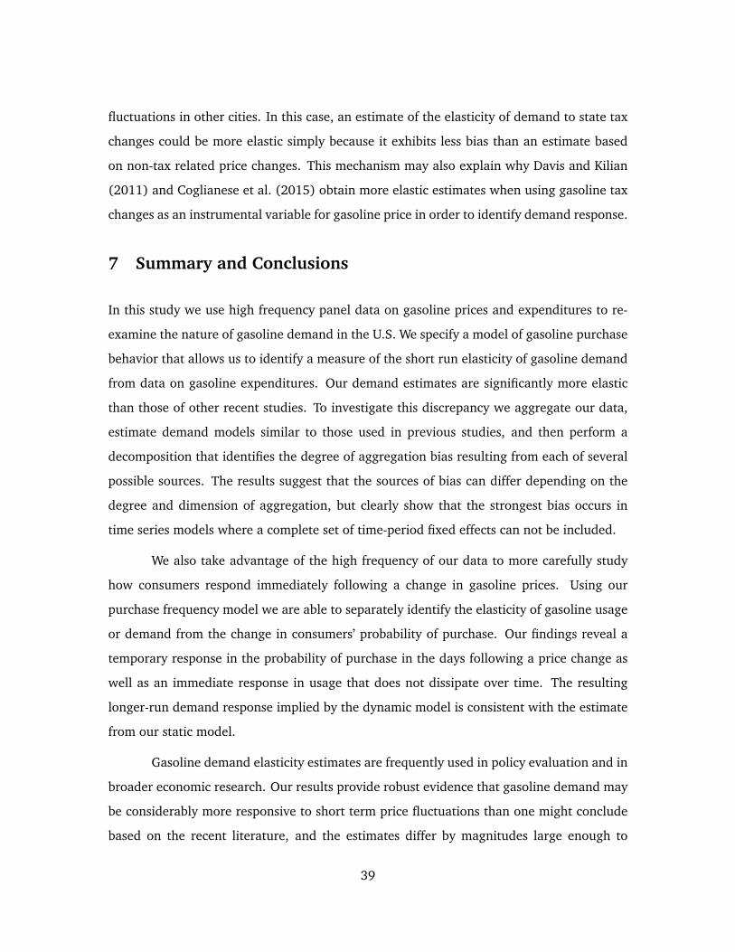
fluctuations in other cities. In this case, an estimate of the elasticity of demand to state tax

changes could be more elastic simply because it exhibits less bias than an estimate based

on non-tax related price changes. This mechanism may also explain why Davis and Kilian

(2011) and Coglianese et al. (2015) obtain more elastic estimates when using gasoline tax

changes as an instrumental variable for gasoline price in order to identify demand response.

7 Summary and Conclusions

In this study we use high frequency panel data on gasoline prices and expenditures to re-

examine the nature of gasoline demand in the U.S. We specify a model of gasoline purchase

behavior that allows us to identify a measure of the short run elasticity of gasoline demand

from data on gasoline expenditures. Our demand estimates are significantly more elastic

than those of other recent studies. To investigate this discrepancy we aggregate our data,

estimate demand models similar to those used in previous studies, and then perform a

decomposition that identifies the degree of aggregation bias resulting from each of several

possible sources. The results suggest that the sources of bias can differ depending on the

degree and dimension of aggregation, but clearly show that the strongest bias occurs in

time series models where a complete set of time-period fixed effects can not be included.

We also take advantage of the high frequency of our data to more carefully study

how consumers respond immediately following a change in gasoline prices. Using our

purchase frequency model we are able to separately identify the elasticity of gasoline usage

or demand from the change in consumers’ probability of purchase. Our findings reveal a

temporary response in the probability of purchase in the days following a price change as

well as an immediate response in usage that does not dissipate over time. The resulting

longer-run demand response implied by the dynamic model is consistent with the estimate

from our static model.

Gasoline demand elasticity estimates are frequently used in policy evaluation and in

broader economic research. Our results provide robust evidence that gasoline demand may

be considerably more responsive to short term price fluctuations than one might conclude

based on the recent literature, and the estimates differ by magnitudes large enough to

39

substantially impact subsequent policy evaluation or market analysis.

Hughes et al. (2008), for example, estimate that gasoline demand has become ex-

tremely inelastic in recent years and conclude that emission reduction goals that rely on

reductions in gasoline consumption will be difficult to achieve using gasoline taxes alone.

They suggest that alternative measures such as CAFE standards may be needed to meet

desired reductions while avoiding politically infeasible tax levels. Based on our more elastic

estimates, however, the required gasoline tax increase needed to achieve a particular reduc-

tion in consumption would be at least 5 times smaller than what would be predicted using

the estimates of Hughes et al. (2008).

Studies evaluating the impacts of cap-and-trade policies, like Borenstein, Bushnell,

Wolak and Zaragoza-Watkins (2015) who analyze expected permit prices under California’s

greenhouse gas emissions cap-and-trade program, also rely directly on existing parameter

estimates such as the price responsiveness of gasoline demand. Partly in response to recent

estimates like those of Hughes et al. (2008), they adopt a rather inelastic value for gaso-

line demand elasticity which may contribute to their overall prediction that the supply of

emissions abatement will be relatively inelastic to permit prices. Acknowledging a greater

elasticity in the demand for gasoline could reduce predicted GHG permit price levels and

volatility.

More accurate elasticity estimates can also substantially impact the inferences one

draws when evaluating the macroeconomic costs of gasoline and oil market disruptions and

the benefits of policies responses like maintaining a Strategic Petroleum Reserve (SPR) that

are intended to reduce these costs. If gasoline demand were significantly more elastic than

previously thought, prices will likely increase substantially less than would otherwise be

predicted in response to a oil supply disruption, and the quantity consumers will purchase

at these prices will be substantially smaller. As a result, the overall macroeconomic dis-

placement effect is likely to be much smaller that would have previously been predicted.

In addition, when consumers have more elastic demand, the release of a certain volume

of fuel from the SPR during a market disruption will not be as effective as a policy lever

aimed at reducing price levels. Our elasticity results strengthen any argument in favor of

40

eliminating or reducing the size of the SPR or mechanisms setting price for greenhouse gas

emissions by demonstrating a significantly larger price-responsiveness of gasoline demand.

In addition to providing a more robust and precise estimate of gasoline demand

response, our aggregation analysis and decomposition of the sources of aggregation bias in

this setting should help researchers and policy analysts to more successfully evaluate the

reliability of existing estimates and to improve empirical design and identification in future

studies.

References

Basso, Leonardo J. and Tae Hoon Oum, “Automobile Fuel Demand: A Critical Assessmentof Empirical Methodologies,” Transport Reviews, 2007, 27 (4), 449–484.

Borenstein, Severin, James Bushnell, Frank A. Wolak, and Matthew Zaragoza-Watkins,“Expecting the Unexpected: Emissions Uncertainty and Environmental Market Design,”Working Paper 20999, National Bureau of Economic Research March 2015.

Brons, Martijn, Peter Nijkamp, Eric Pels, and Piet Rietveld, “A meta-analysis of the priceelasticity of gasoline demand. A {SUR} approach,” Energy Economics, 2008, 30 (5), 2105– 2122.

Coglianese, John, Lucas W. Davis, Lutz Kilian, and James H. Stock, “Anticipation, TaxAvoidance, and the Price Elasticity of Gasoline Demand,” February 2015. National Bureauof Economic Research, Working Paper No. 20980.

Cui, Carolyn, “Questions Arise on Gasoline Data,” The Wall Street Journal, March 21, 2012,p. C1.

Dahl, Carol and Thomas Sterner, “Analysing Gasoline Demand Elasticities: A Survey,”Energy Economics, July 1991, 13 (3), 203–210.

Davis, Lucas W. and Lutz Kilian, “Estimating the Effects of a Gasoline Tax on CarbonEmissions,” Journal of Applied Econometrics, November/December 2011, 26 (7), 1187–1214.

Espey, Molly, “Gasoline Demand Revisited: An International Meta-analysis of Elasticities,”Energy Economics, 1998, 20 (3), 273–295.

Gicheva, Dora, Justine Hastings, and Sofia Villas-Boas, “Revisiting the Income Effect:Gasoline Prices and Grocery Purchases,” November 2007. NBER Working Paper No.13614.

Goodwin, P. B., “A Review of New Demand Elasticities with Special Reference to Short andLong Run Effects of Price Changes,” Journal of Transport Economics and Policy, May 1992,26 (2), 155–169.

41

Hastings, Justine S. and Jesse M. Shapiro, “Fungibility and Consumer Choice: Evidencefrom Commodity Price Shocks*,” The Quarterly Journal of Economics, 2013, 128 (4),1449–1498.

Hsing, Yu, “On the variable elasticity of the demand for gasoline: The case of the {USA},”Energy Economics, 1990, 12 (2), 132 – 136.

Hughes, Jonathan E., Christopher R. Knittel, and Daniel Sperling, “Evidence of a Shiftin the Short-Run Price Elasticity of Gasoline Demand,” The Energy Journal, 2008, 29 (1),93–114.

Li, Shanjun, Joshua Linn, and Erich Muehlegger, “Gasoline Taxes and Consumer Behav-ior,” American Economic Journal: Economic Policy, 2014, 6 (4), 302–42.

Lin, C.-Y. Cynthia and Lea Prince, “Gasoline Price Volatility and the Elasticity of Demandfor Gasoline,” Energy Economics, July 2013, 38, 111–117.

Morath, Eric, “Lower Gas Prices Drove Down Transit Use,” The Wall Street Journal, April 6,2016.

Park, Sung Y. and Guochang Zhao, “An estimation of U.S. gasoline demand: A smoothtime-varying cointegration approach,” Energy Economics, 2010, 32, 110–120.

Rivers, Nicholas and Brandon Schaufele, “Salience of carbon taxes in the gasoline mar-ket,” Journal of Environmental Economics and Management, November 2015, 74, 23 –36.

Small, Kenneth A. and Kurt Van Dender, “Fuel Efficiency and Motor Vehicle Travel: TheDeclining Rebound Effect,” Energy Journal, 2007, 28 (1), 25–51.

Sommer, Jeff, “Cheap Gas Is a Thrill, but a Costly One,” The New York Times, December 11,2015.

Sterner, Thomas and Carol Dahl, “Modeling Transport Fuel Demand,” in Thomas Sterner,ed., International Energy Economics, Chapman-Hall, 1992, pp. 65–79.

42

Appendices

A Exploring Potential Biases due to Substitution from RegularGrade to Premium Grade Gasoline

Our data include daily total revenues at gas stations aggregated to the city level and a city-

level average of regular grade gasoline prices. Our measure of the quantity purchased in

a city on a given day is generated by dividing the aggregate gasoline station revenue by

the average price. One concern with this approach arises from the fact that roughly 15%

of gasoline purchases are purchases of mid-grade or premium grade gasoline which sells

at a higher prices than regular grade. As a result, dividing total revenues (from sales of

all grades) by the price of regular grade gasoline generates a slight overestimate of the

number of total gallons purchased. If the relative shares of premium, mid-grade, and reg-

ular gasoline remains fairly constant over time the presence of premium and mid-grade

purchases would not bias our elasticity estimates, as all identification is based on rela-

tive changes in prices and quantities over time. However, Hastings and Shapiro (2013)

present evidence that gasoline consumers substitute from premium to regular grade fuel

when gasoline prices increase. If the relative purchase shares of regular and premium gaso-

line fluctuate with price this substitution could bias our elasticity estimate. The following

calculation approximates the potential size of such a bias.

Assuming that premium gasoline sells at a γ% premium over the regular grade price,

the true quantity of gasoline purchased can be represented by:

Qtrue =Sreg ∗RPreg

+(1− Sreg) ∗RPreg ∗ (1 + γ)

,

where Sreg is the share of all gasoline purchased that is of regular grade and (1 − Sreg)

represents the share of premium grade purchases, Preg represents the price of regular grade

gasoline, R is the total observed revenues from all gasoline sales. (For simplicity I am

considering just regular and premium grades.)

The measure of quantity we use in the paper does not adjust for the price difference

43

between premium and regular grade sales, so our measure can be expressed as:

Qmeasured =R

Preg≡ Sreg ∗R

Preg+

(1− Sreg) ∗RPreg

.

As a result, the bias in our measure of quantity will simply be:

BiasQ = Qtrue −Qmeasured =(1− Sreg) ∗R

Preg− (1− Sreg) ∗RPreg ∗ (1 + γ)

=γ

1 + γ(1− Sreg) ∗

R

Preg,

where γ1+γ reflects the percentage discount at which regular grade sells relative to premium

grade, and γ1+γ (1 − Sreg) then represents the percent to which our quantity measure is

biased (upward) from the true quantity as a result of assuming that all gasoline is sold at

the regular-grade price.

Once again, if γ and Sreg are constant over time our demand elasticity estimates will

not be affected by this bias. On the other hand, if the share of consumers buying regular

grade gasoline (Sreg) increases when prices rise (as Hastings and Shapiro (2013) suggest)

then some of the decrease in quantity we observe could be a result of people substituting

to cheaper regular grade gasoline rather than people reducing gasoline consumption alto-

gether. The magnitude of this effect, however, is almost sure to be rather small. Hastings

and Shapiro (2013) estimate that a $1.00 increase in the gasoline price is associated with a

1.4 percentage point increase in the share of people buying regular grade gasoline. Given

that prices average around $3.00 per gallon during our sample and the baseline share of

people buying regular grade gasoline is around 85%, this would imply a price elasticity of

substitution to regular grade gasoline of around 0.0005.

Measuring gasoline price in cents per gallon and assuming a mark-up on premium

gasoline of around 10% over regular, this implies that:

∂PercentBiasQ∂Preg

=γ

1 + γ(−∂Sreg∂Preg

) = 0.1 ∗ (−0.014) = −0.0014,

which in the absence of any actual demand response and at an average gasoline price of

$3.00 would generate a false elasticity of demand of around −0.0014 ∗ 3 = −0.0042. Given

that our demand elasticity estimates are two orders of magnitude larger than this, any

substitution from premium to regular gasoline associated with price changes will have a

negligible impact on our analysis.

44

B Exploring the Bias in Estimated Gasoline Demand ElasticityResulting from Non-Gasoline Purchases

As is discussed in Section 3, measuring quantity using the total revenues earned by gas

stations in a city on a particular day divided by the city’s average price of gasoline will

result in upward bias since around 21% of these revenues come from non-gasoline items.

More importantly for our demand analysis, the estimated response of gasoline consumption

to changes in prices will also biased upward (in absolute value). In our analysis we attempt

to avoid this issue by using only pay-at-pump transactions in our quantity calculations.

However, it is also possible to derive a reasonably accurate approximation of the magnitude

of the bias that would result from using all transactions to calculate the quantity of gasoline

sold. In this section we will derive the expected bias and show that it is fairly similar to

the difference in estimated elasticities found when using only pay-at-pump transactions as

opposed to all transactions.

Dividing total revenues by price results in a quantity measure Q̃ = Q + KP , where

Q represents the true quantity of gasoline sold, K represents the revenues from all non-

gasoline sales, and P is the price of gasoline. Using this representation, the response of our

measure of Q to a change in price will be:

∂Q̃

∂P=∂Q

∂P− K(P )

P 2+

1

P

∂K(P )

∂P.

Here we have allowed for the possibility that the demand for non-gasoline items may also

be influenced by changes in the price of gasoline. As a result, the elasticity of our measure

of Q with respect to price will be:

ε̃ =∂Q̃

∂P

P

Q̃=

∂Q

∂P

P

Q+ KP

− K(P )

P 2

P

Q+ KP

+1

P

∂K(P )

∂P

P

Q+ KP

=∂Q

∂P

P

Q

Q

Q+ KP

−KP

Q+ KP

+∂K(P )

∂P

P

K

KP

Q+ KP

= εgσg − (1− σg) + (1− σg) ∗ εk

= εgσg + (1− σg)(εk − 1),

where εg = ∂Q∂P

PQ represents the true elasticity of demand for gasoline, εk = ∂K(P )

∂PPK rep-

resent the elasticity of non-gasoline revenues with respect to the price of gasoline, and

45

σg = PQPQ+K represents the share of total revenues coming from gasoline sales. Alterna-

tively, the true elasticity of demand for gasoline can be expressed as a function of our

all-transactions elasticity estimate:

εg =ε̃

σg+

1− σgσg

(εk − 1).

Based on this result, we can approximate the expected bias using estimates of pa-

rameters from previous studies. A survey of gas station consumers conducted by the Na-

tional Association of Convenience Stores (NACS) estimates that around 27% of gas stations

transactions are in cash, and only 44% of customers enter the store during their visit.25

Assuming that all cash paying customers enter the store, at most 17% of all customers

(or 39% of those entering the store) are potentially making non-gasoline purchases with a

credit card. Data from the U.S. Economic Census suggests that 21% of all gas station rev-

enues come from non-gasoline items. Supposing that gasoline revenues can be attributed

proportionally across all payer types and non-gasoline revenues attributed proportionally

across customers entering the store, this would suggest that non-gasoline purchases repre-

sent roughly 6% of non-cash customers’ total spending.26

There are no direct estimates of how the demand for non-gasoline items at the sta-

tion responds to changes in the price of gasoline, but Gicheva et al. (2007) have examined

how gasoline prices impact consumer spending more generally. They estimate that con-

sumers reduce spending on food away from home by 45-56% when gas prices increase by

100%. However, they also find that grocery spending actually increases as consumers cook

at home more and that consumers substitute from more expensive to less expensive items

within each category. In some ways, food and drink from a gasoline convenience store

can be considered part of the food away from home category, but packaged items from the

convenience store could also be considered as similar to grocery items (or less expensive

options compared with other food away from home). As a result, it could be that spending25See the 2014 NACS Retail Fuels Report (http://www.nacsonline.com/YourBusiness/

FuelsReports/GasPrices_2014/Pages/default.aspx). Survey data from previous years couldnot be used because the question determining the share of customers entering the store was not included.

26The 6% results from multiplying the fraction those visiting the store that do not pay cash times the shareof revenues that are non-gasoline (39% × 21%) and then dividing this by the the overall share of non-cashcustomers times the share of revenues from gasoline (73% × 79%).

46

in convenience stores decreases when gas prices rise, but probably not to the same extent

as other food away from home.

Considering these findings, suppose the share of total credit card customer revenues

coming from gasoline sales (σg) is 94% (= 1 − .06), and the elasticity of non-gasoline

revenues with respect to the price of gasoline (εk) is 33%. Then, based on the bias derived

above and the demand elasticity estimated using all purchases in our data, the true gasoline

demand elasticity can be approximated as:

εg =ε̃

.94− .064 ∗ (−1.33) = 1.064ε̃+ .085.

Interestingly, the bias-adjusted elasticity estimates implied by this relationship are relatively

similar in magnitude to the elasticities obtained by estimating demand using only pay-at-

pump transactions (reported in Table 1). For example, applying this bias-adjustment to

the elasticity estimate of −.328 from the traditional demand model estimated using all

transactions (Column 4) would imply a true elasticity of gasoline of εg = 1.064(−.328) +

.085 = −.264, which is very close to the coefficient of −.259 that we obtain when estimating

the same model using only pay-at-pump transactions (Column 1). The estimate from our

probability of purchase model (Column 6) would imply a bias-adjusted elasticity estimate

of around −.336 which is also much closer to (though not as low as) the estimate of −.288

obtained using only pay-at-pump transactions (Column 3).

We conclude from the calculations above that biases resulting from the presence of

non-gasoline purchases in our data are non-negligible in magnitude but are nowhere near

large enough to explain the differences between our elasticity estimates and those obtained

by other recent studies. Moreover, our ability to estimate demand using only pay-at-pump

purchases appears to eliminate, or perhaps over-correct for, any bias resulting from non-

gasoline purchases.

47

C Instrumental Variables Estimates

Table 6 reports the instrumental variables estimation results for both the basic model (Col-

umn 1) and the restricted and unrestricted versions of the consumer purchase model (Columns

2 & 3) presented in Section 4. All specifications are estimated using only pay-at-pump pur-

chases. In an attempt to utilize exogenous variation refinery market conditions to identify

supply-driven price fluctuations we use the log of the current "spot market" price of gaso-

line in the region as an instrument for local retail prices. While using measures of refinery

outages directly as instruments might seem like attractive alternative, the relationship be-

tween outages and gasoline prices is complex and difficult to capture in a model because the

impact depends also on the level of inventories in the market, the ease of importing from

alternative sources, the available capacity at other refineries in the area, etc. Using spot

market prices reveals the net impact of these outages on gasoline markets. Input prices fur-

ther upstream are also not likely to be useful instruments here, as oil prices do not exhibit

the regional variation necessary to identify fluctuations in relative gasoline prices across

different parts of the country.

We use the spot market gasoline price data reported by the Department of Energy’s

Energy Information Administration for either New York Harbor, the Gulf Coast, or Los An-

geles depending on which of these large refining centers is most closely integrated into the

city’s gasoline supply network. Petroleum Area Defense District (PADD) geographic defini-

tions are used to classify this supply network integration. The New York Harbor spot price is

used as an instrument for cities in the New England and Central Atlantic portions of PADD

1; the Gulf Coast spot price is used for cities in the Lower Atlantic region of PADD 1 and

for cities in PADDs 2, 3, and 4; and the Los Angeles spot price is used for PADD 5 cities.

Resulting estimates are directly comparable to the OLS estimates from Columns 4 through

6 of Table 1.

48

Table 6: IV Estimates of Baseline Empirical Model of Demand

Dependent Variable = ln(quantityjd)Pay-at-Pump Only

(1) (2) (3)ln(pricejd) −0.357 −0.431 −0.323

(0.050) (0.085) (0.017)ln(# of transactionsjd) 1 0.996

(0.002)ln(predicted probability −1 −0.003

of purchasejd) (0.009)Note: Day-of-sample fixed effects and city fixed effects are included in all specifications.

Log retail gasoline prices in each city are instrumented for using the log of the spot price

of gasoline from the either New York Harbor, the Gulf Coast, or Los Angeles depending on

which of these refining centers is most closely linked with the city’s supply infrastructure.

Standard errors in Columns 1 & 4 are robust and clustered to allow serial correlation within

city. Standard errors for the remaining specifications are generated using a nonparametric

bootstrap that allows errors to be serially correlated within a city and jointly distributed with

the error term in the first-stage regression.

D Replication of Hughes et al. (2008) Model and Comparison toVisa Data

Once aggregated to a national time series our elasticity estimates are fairly close to those of

Hughes et al. (2008) who estimate an identical specification using data from 2000–2006.

Although our data is from a later period, we can generate a more accurate comparison by

replicating the same specification using their data sources but for our later time period. As in

their study, gasoline consumption is measured using the EIA’s monthly nationwide estimate

of motor gasoline “product supplied”. Price is measured using the U.S. city average price for

unleaded regular gasoline as reported in the U.S. Bureau of Labor Statistics’ CPI-Average

Price Data and is converted to constant 2005 dollars using the GDP implicit price deflator.

To check our ability to replicate the Hughes et al. (2008) analysis we first estimate

their baseline double-log specification (equivalent to Column 5 of Table 4 above) for the

period 2001–2006. Results are reported in Table 7, Column 1. The estimate of price elastic-

ity (−.042) is identical to that of Hughes et al. (2008).27 Estimating the same specification27Our estimate of the income elasticity is .32 as opposed to their estimate of .53. This discrepancy appears

49

Table 7: Elasticity Estimates from Replication of Hughes et al. (2008)

Dependent Variable = ln(quantity per capita)Date Range: 2000–2006 2006–2009 2006–2009 2006–2009Data Source: EIA/BLS EIA/BLS Visa/AAA Visa/AAA

(all purchases) (pay-at-pump)(1) (2) (3) (4)

ln(pricet) −0.042 0.026 −0.122 0.004(0.010) (0.024) (0.016) (0.017)

ln(incomet) 0.321 −1.272 0.154 0.093(0.066) (0.405) (0.167) (0.189)

Month-of-Year X X X XFixed Effects

Note: Columns (1) and (2) use EIA data on “product supplied” to measure quantity and the CPI average price

data for unleaded regular to measure price. Column (3) uses our Visa expenditure data to measure quantity

and a weighted average of our AAA average price data to measure price. Standard errors are estimated using a

Newey-West procedure and are robust to serial correlation.

using data from 2006–2009 yields a price elasticity that is slightly positive and not signifi-

cantly different from zero. This is very similar to our estimate from the same specification

using aggregated Visa pay-at-pump purchase data (reported in Column 4) but is much less

elastic than our estimate using all Visa purchases (Column 3). The use of an alternative

data source may be partially responsible for differences between our elasticity estimates

and those of previous studies, but overall the results above suggest that most of the differ-

ence likely a result of the level of data aggregation.

to have been caused by the fact that Hughes et al. (2008) use previously published estimates of disposablepersonal income that have since been revised by the BEA. We utilize the updated estimates so that our incomemeasures are consistent with those available for the 2006–2009 sample period.

50

E Additional Figures

Figure 3: Day-of-Week Averages of Daily Nationwide Gasoline Expenditures by Visa Cus-tomers in our 243 Cities

$200

$220

$240

$260

$280

$300

$320

Dol

lars

in M

illio

ns

Sunday Monday Tuesday Wednesday Thursday Friday Saturday

Day of Week

Figure 4: Day-of-Week Averages of Nationwide Gasoline Expenditures per Transaction byVisa Customers in our 243 Cities

$25.75

$26.00

$26.25

$26.50

$26.75

Dol

lars

Per

Tra

nsac

tion

Sunday Monday Tuesday Wednesday Thursday Friday Saturday

Day of Week51