Electronic copy available at: http://ssrn.com/abstract=1641387

HIGH FREQUENCY TRADING AND ITSIMPACT ON MARKET QUALITY

Jonathan A. Brogaard ∗

Northwestern UniversityKellogg School of Management

Northwestern University School of Lawj-brogaard@kellogg.northwestern.edu

July 16, 2010

∗I would like to thank my advisors, Tom Brennan, Robert Korajczyk, Robert McDonald, An-nette Vissing-Jorgensen for the considerable amount of time and energy they spent discussing thistopic with me. I would like to thank Nasdaq OMX for making available the data used in thisproject. Also, I would like to thank the many other professors and Ph.D. students at NorthwesternUniversity’s Kellogg School of Management and at Northwestern’s School of Law for assistanceon this paper. Please contact the author before citing this preliminary work.

1

Electronic copy available at: http://ssrn.com/abstract=1641387

Abstract

This paper examines the impact of high frequency traders (HFTs) onequities markets. I analyze a unique data set to study the strategies uti-lized by HFTs, their profitability, and their relationship with characteristicsof the overall market, including liquidity, price efficiency, and volatility. Ifind that in my sample HFTs participate in 77% of all trades and that theytend to engage in a price-reversal strategy. I find no evidence suggestingHFT withdraw from markets in bad times or that they engage in abnormalfront-running of large non-HFT trades. The 26 HFT firms in the sampleearn approximately $3 billion in profits annually. HFTs demand liquidityfor 50.4% of all trades and supply liquidity for 51.4% of all trades. HFTstend to demand liquidity in smaller amounts, and trades before and aftera HFT demanded trade occur more quickly than other trades. HFTs pro-vide the inside quotes approximately 50% of the time. In addition if HFTswere not part of the market, the average trade of 100 shares would resultin a price movement of $.013 more than it currently does, while a trade of1000 shares would cause the price to move an additional $.056. HFTs arean integral part of the price discovery process and price efficiency. Utiliz-ing a variety of measures introduced by Hasbrouck (1991a, 1991b, 1995),I show that HFT trades and quotes contribute more to price discovery thando non-HFT activity. Finally, HFT reduces volatility. By constructing ahypothetical alternative price path that removes HFTs from the market, Ishow that the volatility of stocks is roughly unchanged when HFT initiatedtrades are eliminated and significantly higher when all types of HFT tradesare removed.

2

Electronic copy available at: http://ssrn.com/abstract=1641387

1 Introduction

1.1 Motivation

On May 6, 2010 the Dow Jones Industrial Average dropped over 1,000 points inintraday trading in what has come to be known as the “flash crash”. The nextday, some media blamed high frequency traders (HFTs; HFT is also used to referto high frequency trading) for driving the market down (Krudy, June 10, 2010).Others in the media blamed the temporary withdrawal of HFTs from the market ascausing the precipitous fall (Creswell, May 16, 2010).1 HFTs have come to makeup a large portion of the U.S. equity markets, yet the evidence of their role in thefinancial markets has come from news articles and anecdotal stories. The SEC hasalso been interested in the issue. It issued a Concept Release regarding the topicon January 14, 2010 requesting feedback on how HFTs operate and what benefitsand costs they bring with them (Securities and Commission, January 14, 2010).

In addition, the Dodd Frank Wall Street Reform and Consumer Protection Actcalls for an in depth study on HFT (Section 967(2)(D)). In this paper I examine theempirical consequences of HFT on market functionality. I utilize a unique datasetfrom Nasdaq OMX that distinguishes HFT from non-HFT quotes and trades. Thispaper provides an analysis of HFT behavior and its impact on financial markets.Such an analysis is necessary since to ensure properly functioning financial mar-kets the SEC and exchanges must set appropriate rules for traders. These rulesshould be based on the actual behavior of actors and not on hearsay and anecdotalstories. It is equally important that institutional and retail investors understandwhether or not they are being manipulated or exploited by sophisticated traders,such as HFT.

This paper studies HFT from a variety of viewpoints. First, it describes theactivities of HFTs, showing that HFTs make up a large percent of all trading andthat they both provide liquidity and demand liquidity. Their activities tend to bestable over time. Second, it examines HFT strategy and profitability. HFTs gen-erally engage in a price reversal strategy, buying after price declines and sellingafter price gains. They are profitable, making around $3 billion each year on trad-ing volume of $30 trillion dollars traded. Third, it considers the impact of HFTson the market, focusing on three areas - liquidity, price discovery, and volatility.HFTs increase market liquidity: using a variety of Hasbrouck measures, I find thatHFTs appear to add to the efficiency of the markets. Finally, I find that HFTs tendto decrease volatility.

1To date, the true cause of the flash crash has not been determined.

3

Given these results, HFT appear to be a new form of market makers. HFTsappear to make markets operate better (i.e. increase liquidity and price efficiency,and reduce volatility) for all market participants.

HFT is a recent phenomenon. Tradebot, a large player in the field who fre-quently makes up over 5% of all trading activity, states that the strategy of HFThas only been around for the last ten years (starting in 1999). Whereas only re-cently an average trade on the NYSE took ten seconds to execute, (Hendershottand Moulton, 2007), now some firms entire trading strategy is to buy and sellstocks multiple times within a mere second. The acceleration in speed has arisenfor two main reasons: First, the change from stock prices trading in eighths todecimalization has allowed for more minute price variation. This smaller pricevariation makes trading with short horizons less risky as price movements are inpennies not eighths of a dollar. Second, there have been technological advancesin the ability and speed to analyze information and to transport data between lo-cations. As a result, a new type of trader has evolved to take advantage of theseadvances: the high frequency trader. Because the trading process is the basis bywhich information and risk become embedded into stock prices it is important tounderstand how HFT is being utilized and its place in the price formation process.

1.2 Definitions

To date, there lacks a clear definition for many of the terms in rapid trading andin computer controlled trading. Even the Securities and Exchange recognizes thisand says that high frequency trading “does not have a settled definition and mayencompass a variety of strategies in addition to passive market making” (Secu-rities and Commission, January 14, 2010). High frequency trading is a type ofstrategy that is engaged in buying and selling shares rapidly, often in terms of mil-liseconds and seconds. This paper takes the definition from the SEC: HFT refersto, “professional traders acting in a proprietary capacity that engages in strategiesthat generate a large number of trades on a daily basis” (Securities and Commis-sion, January 14, 2010). By some estimates HFT makes up over 50% of the totalvolume on equity markets daily (Securities and Commission, January 14, 2010;Spicer, December 2, 2009).

Other terms of interest when discussing HFT include “pinging” and “algorith-mic trading.”

The SEC defines pinging as, “an immediate-or-cancel order that can be usedto search for and access all types of undisplayed liquidity, including dark poolsand undisplayed order types at exchanges and ECNs. The trading center thatreceives an immediate-or-cancel order will execute the order immediately if it has

4

available liquidity at or better than the limit price of the order and otherwise willimmediately respond to the order with a cancelation” (Securities and Commission,January 14, 2010). The SEC goes on to clarify, “[T]here is an important distinctionbetween using tools such as pinging orders as part of a normal search for liquiditywith which to trade and using such tools to detect and trade in front of largetrading interest as part of an ‘order anticipation’ trading strategy” (Securities andCommission, January 14, 2010).

A type of trading that is similar to HFT, but fundamentally different is algorith-mic trading. Algorithmic Trading is defined as “”the use of computer algorithmsto automatically make trading decisions, submit orders, and manage those ordersafter submission” (Hendershott and Riordan, 2009). Algorithmic and HFT aresimilar in that they both use automatic computer generated decision making tech-nology. However, they differ in that algorithmic trading may have holding periodsthat are minutes, days, weeks, or longer, whereas HFT by definition hold theirposition for a very short horizon and try and to close the trading day in a neutralposition. Thus, HFT must be a type of algorithmic trading, but algorithmic tradingneed not be HFT.

2 Literature ReviewHFT has received little attention to date in the academic literature. This is be-cause until recently the concept of HFT did not exist. In addition, data to conductresearch in this area has not been available. The only academic paper regardingHFT is one by Kearns, Kulesza, and Nevmyvaka (2010), and this paper showsthat the maximum amount of profitability that HFT can make based on TAQ dataunder the implausible assumption that HFT enter every transaction that is prof-itable. The findings suggest that an upper bound on the profits HFT can earn peryear is $21.3 billion. Although my research is the first to look at the impact ofHFT on the stock market, it touches on a variety of related fields of research, themost relevant being algorithmic trading.

2.1 Algorithmic Trading

In principal algorithmic trading is similar to HFT except that the holding periodcan vary. It is also similar to HFT in that data to study the phenomena are difficultto obtain. Nonetheless several papers have studied algorithmic trading (AT).

Hendershott and Riordan (2009) use data from the firms listed on the DeutscheBoerse DAX. They find that AT supply 50% of the liquidity in that market. Theyfind that AT increase the efficiency of the price process and that AT contribute

5

more to price discovery than does human trading. Also, they find a positive re-lationship between AT providing the best quotes for stocks and the size of thespread. Regarding volatility, the study finds little evidence between any relation-ship between it and AT.

Hendershott, Jones, and Menkveld (2008) utilize a dataset of NYSE electronicmessage traffic, and use this as a proxy for algorithmic liquidity supply. Thetime period of their data surrounds the start of autoquoting on NYSE for differentstocks and so they use this event as an exogenous instrument for AT. The studyfinds that AT increases liquidity and lowers bid-ask spreads.

Chaboud, Hjalmarsson, Vega, and Chiquoine (2009) look at AT in the foreignexchange market. Like Hendershott and Riordan (2009), they find no evidenceof there being a causal relationship between AT and price volatility of exchangerates. Their results suggest human order flow is responsible for a larger portion ofthe return variance.

Together these papers suggest that algorithmic trading as a whole improvesmarket liquidity and does not impact, or may even decrease, price volatility. Thispaper fits in to this literature by decomposing the AT type traders into short-horizon traders and others and focusing on the impact of the short-horizon traderson market quality.

2.2 Theory

There is an extant literature in theoretical asset pricing. Of these papers only ahandful try to understand what the impact on market quality will be of havinginvestors with different investment time horizons. Two papers directly addressthe scenario when there are short and long term investors in a market: “Herd onthe Street: Informational Inefficiencies in a Market with Short-Term Speculation”(Froot, Scharfstein, and Stein, 1992); and “Short-Term Investment and the Infor-mational Efficiency of the Market” (Vives, 1995).

Froot, Scharfstein, and Stein (1992) find that short-term speculators may puttoo much emphasis on some (short term) information and not enough on funda-mentals. The result being a decrease in the informational quality of asset prices.Although the paper does not extend its model in the following direction, a de-crease in the informational quality suggests a decrease in price efficiency and anincrease in volatility.

Vives (1995) obtains the result that the market impact of short term investorsdepends on how information arrives. The informativeness of asset prices is im-pacted differently based on the arrival of information, “with concentrated arrivalof information, short horizons reduce final price informativeness; with diffuse ar-

6

rival of information, short horizons enhance it” (Vives, 1995). The theoreticalwork on short horizon investors suggest that HFT may be beneficial to marketquality or may be harmful to it.

3 Data

3.1 Standard Data

The data in this paper comes from a variety of sources. It uses in standard fash-ion CRSP data when considering daily data not included in the Nasdaq dataset.Compustat data is used to incorporate firm characteristics in the analysis.

3.2 Nasdaq High Frequency Data

The unique data set used in this study has data on trades and quotes on a groupof 120 stocks. The trade data consists of all trades that occur on the Nasdaq ex-change, excluding trades that occurred at the opening, closing, and during intradaycrosses. The trade date used in this study includes those from all of 2008, 2009and from February 22, 2010 to February 26, 2010. The trades include a millisec-ond timestamp at which the trade occurred and an indicator of what type of trader(HFT or not) is providing or taking liquidity.

The Quote data is from February 22, 2010 to February 26, 2010. It includesthe best bid and ask that is being offered by HFT firms and by non-HFT firms atall times throughout the day.

The Book data is from the first full week of the first month of each quarterin 2008 and 2009, September 15 - 19, 2008, and February 22 - 26, 2010. Itprovides the 10 best price levels on each side of the market that are available onthe Nasdaq book. Along with the standard variables for limit order data, the datashow whether the liquidity is provided by a HFT or a non-HFT, and whether theliquidity was displayed or hidden.

The Nasdaq dataset consists of 26 traders that have been identified as engag-ing primarily in high frequency trading. This was determined based on knowninformation regarding the different firms’ trading styles and also on the firms’website descriptions. The characteristics of HFT firms that are identified are thefollowing: They engage in proprietary trading; that is, the firm does not havecustomers but instead trades its own capital. The HFT use sophisticated tradingtools such as high-powered analytics and computing co-location services locatednear exchanges to reduce latency. The HFT engage in sponsored access providerswhereby they have access to the co-location services and can obtain large-volumediscounts. HFT tend to use OUCH protocol whereas non-HFT tend to use RASH.

7

The HFT firms tend to switch between long and short net positions several timesthroughout the day, whereas non-HFT labeled firms rarely switch from long toshort net positions on any given day. Orders by HFT firms are of a shorter timeduration than those placed by non-HFT firms. Also, HFT firms normally have alower ratio of trades per orders placed than for non-HFT firms.

Firms that others may define as HFT are not labeled as HFT firms here if theysatisfy one of the following: firms like Lime Brokerage and Swift Trade who pro-vide direct market access and other powerful trading tools to its customers, whoare likely engaging in HFT and thus are likely HFT traders but are not labeled so;proprietary trading firms that are a desk of a larger, integrated firm, like GoldmanSachs or JP Morgan; an independent firm that is engaged in HFT activities, butwho routes its trades through a MPID of a non-HFT type firm; firms that engagein HFT activities but because they are small are not considered in the study asbeing labeled a HFT firm.

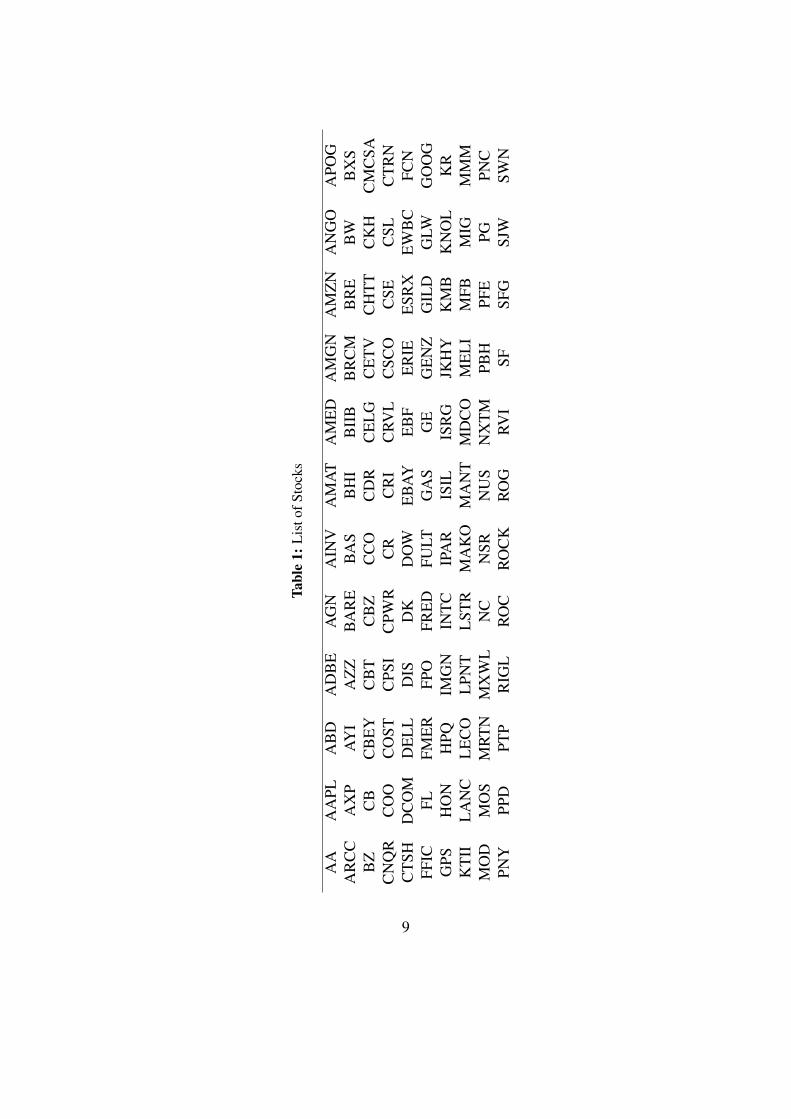
The data is for a sample of 120 Nasdaq stocks where the ticker symbols arelisted in Table 1. These sample stocks were selected by a group of academics. Thestocks consist of a varying degree of market capitalization, market-to-book ratios,industries, and listing venues.

4 Descriptive StatisticsBefore entering the analysis section of the paper, as HFT data has not been iden-tified before, I first provide the basic descriptive statistics of interest. I look at liq-uidity and trading statistics of the HFT sample and show they are typical stocks,I then compare the firm characteristics to the Compustat database and show theyare on average larger firms, but otherwise a relatively close match to an averageCompustat firm. Finally, I provide general statistics on the percent of the mar-ket trades in which HFT are involved, considering all types of trades, supplyingliquidity trades, and demanding liquidity trades.

Table 2 describes the 120 stocks in the Nasdaq sample data set. These statisticsare taken for the five trading days from February 22 to February 26, 2010. Thistable shows that these stocks are quite average and provide a reasonable subsampleof the market. The price of the stocks is on average 39.57 and ranges between 4.6and 544. The daily trading volume on Nasdaq for these stocks averages 1.064million shares, and ranges from as small as 2,000 shares to 14 million shares.This is done on average over 5,150 trades, whereas some stock trade just 8 timeson a given day while others trade as many as 59,799 times. The 120 stocks arequite liquid. Quoted half-spreads are calculated when trades occur. the average

8

Tabl

e1:

Lis

tofS

tock

s

AA

AA

PLA

BD

AD

BE

AG

NA

INV

AM

AT

AM

ED

AM

GN

AM

ZN

AN

GO

APO

GA

RC

CA

XP

AY

IA

ZZ

BA

RE

BA

SB

HI

BII

BB

RC

MB

RE

BW

BX

SB

ZC

BC

BE

YC

BT

CB

ZC

CO

CD

RC

EL

GC

ET

VC

HT

TC

KH

CM

CSA

CN

QR

CO

OC

OST

CPS

IC

PWR

CR

CR

IC

RVL

CSC

OC

SEC

SLC

TR

NC

TSH

DC

OM

DE

LL

DIS

DK

DO

WE

BA

YE

BF

ER

IEE

SRX

EW

BC

FCN

FFIC

FLFM

ER

FPO

FRE

DFU

LTG

AS

GE

GE

NZ

GIL

DG

LWG

OO

GG

PSH

ON

HPQ

IMG

NIN

TC

IPA

RIS

ILIS

RG

JKH

YK

MB

KN

OL

KR

KT

IIL

AN

CL

EC

OL

PNT

LST

RM

AK

OM

AN

TM

DC

OM

EL

IM

FBM

IGM

MM

MO

DM

OS

MR

TN

MX

WL

NC

NSR

NU

SN

XT

MPB

HPF

EPG

PNC

PNY

PPD

PTP

RIG

LR

OC

RO

CK

RO

GRV

ISF

SFG

SJW

SWN

9

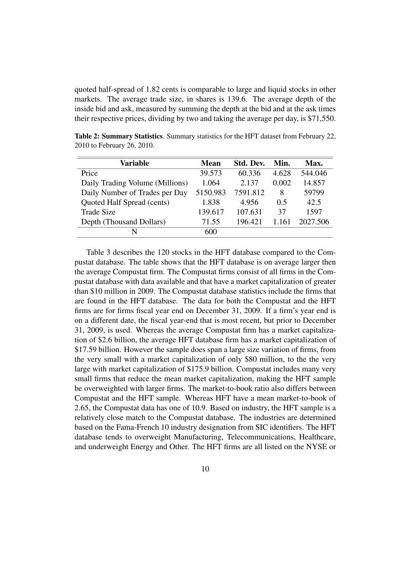
quoted half-spread of 1.82 cents is comparable to large and liquid stocks in othermarkets. The average trade size, in shares is 139.6. The average depth of theinside bid and ask, measured by summing the depth at the bid and at the ask timestheir respective prices, dividing by two and taking the average per day, is $71,550.

Table 2: Summary Statistics. Summary statistics for the HFT dataset from February 22,2010 to February 26, 2010.

Variable Mean Std. Dev. Min. Max.Price 39.573 60.336 4.628 544.046Daily Trading Volume (Millions) 1.064 2.137 0.002 14.857Daily Number of Trades per Day 5150.983 7591.812 8 59799Quoted Half Spread (cents) 1.838 4.956 0.5 42.5Trade Size 139.617 107.631 37 1597Depth (Thousand Dollars) 71.55 196.421 1.161 2027.506

N 600

Table 3 describes the 120 stocks in the HFT database compared to the Com-pustat database. The table shows that the HFT database is on average larger thenthe average Compustat firm. The Compustat firms consist of all firms in the Com-pustat database with data available and that have a market capitalization of greaterthan $10 million in 2009. The Compustat database statistics include the firms thatare found in the HFT database. The data for both the Compustat and the HFTfirms are for firms fiscal year end on December 31, 2009. If a firm’s year end ison a different date, the fiscal year-end that is most recent, but prior to December31, 2009, is used. Whereas the average Compustat firm has a market capitaliza-tion of $2.6 billion, the average HFT database firm has a market capitalization of$17.59 billion. However the sample does span a large size variation of firms, fromthe very small with a market capitalization of only $80 million, to the the verylarge with market capitalization of $175.9 billion. Compustat includes many verysmall firms that reduce the mean market capitalization, making the HFT samplebe overweighted with larger firms. The market-to-book ratio also differs betweenCompustat and the HFT sample. Whereas HFT have a mean market-to-book of2.65, the Compustat data has one of 10.9. Based on industry, the HFT sample is arelatively close match to the Compustat database. The industries are determinedbased on the Fama-French 10 industry designation from SIC identifiers. The HFTdatabase tends to overweight Manufacturing, Telecommunications, Healthcare,and underweight Energy and Other. The HFT firms are all listed on the NYSE or

10

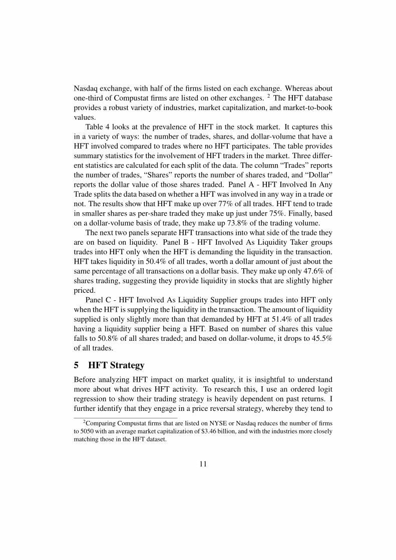
Nasdaq exchange, with half of the firms listed on each exchange. Whereas aboutone-third of Compustat firms are listed on other exchanges. 2 The HFT databaseprovides a robust variety of industries, market capitalization, and market-to-bookvalues.

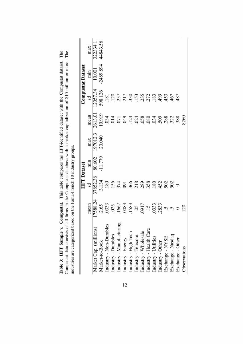
Table 4 looks at the prevalence of HFT in the stock market. It captures thisin a variety of ways: the number of trades, shares, and dollar-volume that have aHFT involved compared to trades where no HFT participates. The table providessummary statistics for the involvement of HFT traders in the market. Three differ-ent statistics are calculated for each split of the data. The column “Trades” reportsthe number of trades, “Shares” reports the number of shares traded, and “Dollar”reports the dollar value of those shares traded. Panel A - HFT Involved In AnyTrade splits the data based on whether a HFT was involved in any way in a trade ornot. The results show that HFT make up over 77% of all trades. HFT tend to tradein smaller shares as per-share traded they make up just under 75%. Finally, basedon a dollar-volume basis of trade, they make up 73.8% of the trading volume.

The next two panels separate HFT transactions into what side of the trade theyare on based on liquidity. Panel B - HFT Involved As Liquidity Taker groupstrades into HFT only when the HFT is demanding the liquidity in the transaction.HFT takes liquidity in 50.4% of all trades, worth a dollar amount of just about thesame percentage of all transactions on a dollar basis. They make up only 47.6% ofshares trading, suggesting they provide liquidity in stocks that are slightly higherpriced.

Panel C - HFT Involved As Liquidity Supplier groups trades into HFT onlywhen the HFT is supplying the liquidity in the transaction. The amount of liquiditysupplied is only slightly more than that demanded by HFT at 51.4% of all tradeshaving a liquidity supplier being a HFT. Based on number of shares this valuefalls to 50.8% of all shares traded; and based on dollar-volume, it drops to 45.5%of all trades.

5 HFT StrategyBefore analyzing HFT impact on market quality, it is insightful to understandmore about what drives HFT activity. To research this, I use an ordered logitregression to show their trading strategy is heavily dependent on past returns. Ifurther identify that they engage in a price reversal strategy, whereby they tend to

2Comparing Compustat firms that are listed on NYSE or Nasdaq reduces the number of firmsto 5050 with an average market capitalization of $3.46 billion, and with the industries more closelymatching those in the HFT dataset.

11

Tabl

e3:

HFT

Sam

ple

v.C

ompu

stat

.T

his

tabl

eco

mpa

res

the

HFT

-ide

ntifi

edda

tase

tw

ithth

eC

ompu

stat

data

set.

The

Com

pust

atda

taco

nsis

tsof

all

firm

sin

the

Com

pust

atda

taba

sew

itha

mar

ket

capi

taliz

atio

nof

$10

mill

ion

orm

ore.

The

indu

stri

esar

eca

tego

rize

dba

sed

onth

eFa

ma-

Fren

ch10

indu

stry

grou

ps.

HFT

Dat

aset

Com

pust

atD

atas

etm

ean

sdm

inm

axm

ean

sdm

inm

axM

arke

tCap

.(m

illio

ns)

1758

8.24

3785

2.38

80.6

0219

7012

.326

13.0

112

057.

3410

.001

3223

34.1

Mar

ket-

to-B

ook

2.65

3.13

4-1

1.77

920

.040

10.9

1959

8.12

6-2

489.

894

4484

3.56

Indu

stry

-Non

-Dur

able

s.0

333

.180

.034

.181

Indu

stry

-Dur

able

s.0

25.1

56.0

14.1

20In

dust

ry-M

anuf

actu

ring

.166

7.3

74.0

71.2

57In

dust

ry-E

nerg

y.0

083

.091

.049

.217

Indu

stry

-Hig

hTe

ch.1

583

.366

.124

.330

Indu

stry

-Tel

ecom

..0

5.2

18.0

24.1

53In

dust

ry-W

hole

sale

.091

7.2

89.0

58.2

35In

dust

ry-H

ealth

Car

e.1

5.3

58.0

80.2

72In

dust

ry-U

tiliti

es.0

333

.180

.034

.183

Indu

stry

-Oth

er.2

833

.452

.509

.499

Exc

hang

e-N

YSE

.5.5

02.2

88.4

53E

xcha

nge

-Nas

daq

.5.5

02.3

22.4

67E

xcha

nge

-Oth

er0

0.3

88.4

87O

bser

vatio

ns12

082

60

12

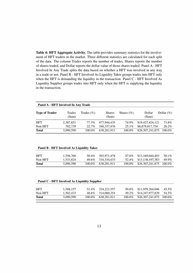
Table 4: HFT Aggregate Activity. The table provides summary statistics for the involve-ment of HFT traders in the market. Three different statistics are calculated for each splitof the data. The column Trades reports the number of trades, Shares reports the numberof shares traded, and Dollar reports the dollar value of those shares traded. Panel A - HFTInvolved In Any Trade splits the data based on whether a HFT was involved in any wayin a trade or not. Panel B - HFT Involved As Liquidity Taker groups trades into HFT onlywhen the HFT is demanding the liquidity in the transaction. Panel C - HFT Involved AsLiquidity Supplier groups trades into HFT only when the HFT is supplying the liquidityin the transaction.

Panel A - HFT Involved In Any Trade

Type of Trader Trades(Sum)

Trades (%) Shares(Sum)

Shares (%) Dollar(Sum)

Dollar (%)

HFT 2,387,851 77.3% 477,944,435 74.9% $19,427,424,121 73.8%Non HFT 702,739 22.7% 160,337,476 25.1% $6,879,817,754 26.2%Total 3,090,590 100.0% 638,281,911 100.0% $26,307,241,875 100.0%

Panel B - HFT Involved As Liquidity Taker

HFT 1,556,766 50.4% 303,971,478 47.6% $13,169,044,493 50.1%Non HFT 1,533,824 49.6% 334,310,433 52.4% $13,138,197,383 49.9%Total 3,090,590 100.0% 638,281,911 100.0% $26,307,241,875 100.0%

Panel C - HFT Involved As Liquidity Supplier

HFT 1,588,157 51.4% 324,221,557 50.8% $11,959,264,046 45.5%Non HFT 1,502,433 48.6% 314,060,354 49.2% $14,347,977,829 54.5%Total 3,090,590 100.0% 638,281,911 100.0% $26,307,241,875 100.0%

13

buy stocks at short-term troughs and they tend to sell stocks at short-term peaks.This is true regardless of whether they are supplying or demanding liquidity. Also,HFT tend to trade in larger, value firms, with lower volume and lower spreads anddepth. Finally, based on their trading activities at the aggregate level I estimatethey earn approximately $3 billion a year.

5.1 Investment Strategy

HFT do not readily share their trading strategies. However, the anecdotal storiesof HFT firms suggest they have essentially replaced the role of market makers byproviding liquidity and a continuous market into which other investors can trade.

What is known regarding HFT is that they tend to buy and sell in very shorttime periods. Therefore, rather than changes in firm fundamentals, HFT firmsmust be basing their decision to buy and sell from short term signals such as stockprice movements, spreads, or volume.

I begin the analysis by performing an all-inclusive ordered logit regressioninto the potentially important factors; thereafter I analyze the promising strategiesin more detail. There are three decisions a HFT firm makes at any given moment:Does it buy, does it sell, or does it do nothing. This decision making processoccurs continuously. I model this setting by using a three level ordered logit. Theordered logit is such that the lowest decision is to sell, the middle option is to donothing, and the highest option is to buy.

Before getting to the ordered logit, I summarize the theoretical reason for whyan ordered logit is appropriate in this setting, as first discussed by Hausman, Lo,and MacKinlay (1992).

HFT trading behavior consist of a sequence of actions Z(t1), Z(t2), . . . , Z(tη)observed at regular time intervals t0, t1, t2, . . . , tη. Let Z∗

k be an unobservablecontinuous random variable where

Z∗k = X

′

kβ + εk, E[εk|Xk] = 0, εk i.n.i.d. N(0, σ2k) (1)

where ‘i.n.i.d.’ stands for the assumption that the εk’s are independent but notidentically distributed, and Xk is a q × 1 vector of predetermined variables thatsets the conditional mean of Z∗

k . Whereas Hausman, Lo, and MacKinlay (1992)deal with tick by tick stock price data, the scenario in this paper deals with HFTtrade behavior data that is aggregated into ten second intervals. Therefore, thesubscripts are used to denote ten second period, not transaction time.

The essence of the ordered logit model is the assumption that observed HFTbehavior Zk are related to the continuous variable Z∗

k in the following mapping:

14

Zk =

s1 if Z∗

k ∈ A1,s2 if Z∗

k ∈ A2,...

...sm if Z∗

k ∈ Am,

where the sets Aj form a partition of the state space ζ∗ of Z∗k . The partition

will have the properties that ζ∗ =∪m

j=1Aj and Ai∩Aj = ∅ for i ̸= j, and the sj’sare the discrete values that comprise the state space ζ of Zk. The ordered logitspecification allows an investigator to understand the link between ζ∗ and ζ andrelate it to a set of economic variables used as explanatory variables that can beused to understand the HFT trading strategy. In this application the sj’s are Sell,Do Nothing, Buy. Note, the observable actions could also be split into size, forexample, Sell 1000 + shares, Sell 500 - 1000, etc., but I restrict the ζ partition tothese three natural breaks. The alternative fine tuned separation, for instance, bysubdividing the buys and selling into the number of shares exchanged, is beyondthe needs of this analysis.

I assume the error terms in εk’s in equation 1 are conditionally independently,but not identically, distributed, conditioned on the Xk’s and the other explanatoryvariables, Wk, that are omitted from equation 1, which allows for heteroscedas-ticity in σ2

k.The conditional distribution of observed return changes Zk, conditioned on

Xk and Wk, is determined by the partition boundaries calculated from the orderedlogit regression. As stated in Hausman, Lo, and MacKinlay (1992), for a Gaussianεk, the conditional distribution is

P (Zk = si|Xk,Wk)

= P (X′

kβ + εk ∈ Ai|Xk,Wk)

=

P (X

′

kβ + εk ≤ α1|Xk,Wk) if i = 1P (αi−1 < X

′

kβ + εk ≤ αi|Xk,Wk) if 1 < i < m,P (αm−1 < X

′

kβ + εk|Xk,Wk) if i = m,(2)

15

=

Φ(

α1−X′kβ

σk) if i = 1

Φ(αi−X

′kβ

σk)− Φ(

αi−1−X′kβ

σk) if 1 < i < m,

1− Φ(αm−1−X

′kβ

σk) if i = m,

(3)

where Φ(·) is the standard normal cumulative distribution function.The intuition for the ordered logit model is that the probability of the type of

behavior by the HFT is determined by where the conditional mean lies relative tothe partition boundaries. Therefore, for a given conditional meanX ′

kβ, shifting theboundaries will alter the probabilities of observing each state, Sell, Do Nothing,or Buy. The order of the outcomes could be reversed with no real consequenceexcept for the coefficients changing signs as the ordered logit only takes advantageof the fact there is some natural ordering of the events. The explanatory variablesthen allow one to analyze the different effects of relevant economic variables tounderstand HFT behavior . As the data determines where the partition boundariesthe ordered logit model creates an empirical mapping between the unobservableζ∗ state space and the observable ζ state space. Here, the empirical relationshipbetween HFT behavior can be analyzed with respect to the economic variablesXk

and Wk.I divide the time frames in to ten second intervals throughout the trading day.

3 For each ten second interval I utilize a variety of independent variables. Theregression I run is as follows:

HFTi,t = α +β1−11 × retlagi,0−10 +β12−22 × depthbidlagi,0−10

+β23−33 × depthasklagi,0−10 +β34−44 × spreadlagi,0−10

+β45−55 × tradeslagi,0−10 β56−66 × dollarvlagi,0−10

Each explanatory variable and its associated beta coefficient has a subscript0-10. This represents the number of lagged time periods away from the eventoccurring in the time t dependent variable. Subscript 0 represents the contempo-

3I also tried other time intervals, such as 250 milliseconds, one second and 100 second periods.The results from these alternative suggestions are similar in significance to the results presentedin that where a ten second period shows significance, so does the one second interval for tenlagged period’s worth, and similarly where ten lagged ten second intervals show significance, sodoes the one lagged one hundred second interval. The ten second intervals has been adopted afterattempting a variety of alterations but finding this one the best for keeping the results parsimoniousand still being able to uncover important results.

16

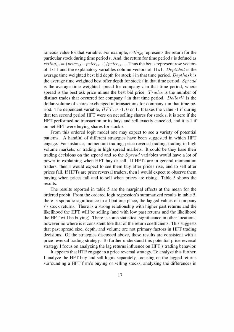
raneous value for that variable. For example, retlag0 represents the return for theparticular stock during time period t. And, the return for time period t is defined asretlagi,0 = (pricei,t−pricei,t−1)/pricei,t−1. Thus the betas represent row vectorsof 1x11 and the explanatory variables column vectors of 11x1. Depthbid is theaverage time weighted best bid depth for stock i in that time period. Depthask isthe average time weighted best offer depth for stock i in that time period. Spreadis the average time weighted spread for company i in that time period, wherespread is the best ask price minus the best bid price. Trades is the number ofdistinct trades that occurred for company i in that time period. DollarV is thedollar-volume of shares exchanged in transactions for company i in that time pe-riod. The dependent variable, HFT , is -1, 0 or 1. It takes the value -1 if duringthat ten second period HFT were on net selling shares for stock i, it is zero if theHFT performed no transaction or its buys and sell exactly canceled, and it is 1 ifon net HFT were buying shares for stock i.

From this ordered logit model one may expect to see a variety of potentialpatterns. A handful of different strategies have been suggested in which HFTengage. For instance, momentum trading, price reversal trading, trading in highvolume markets, or trading in high spread markets. It could be they base theirtrading decisions on the srpead and so the Spread variables would have a lot ofpower in explaining when HFT buy or sell. If HFTs are in general momentumtraders, then I would expect to see them buy after prices rise, and to sell afterprices fall. If HFTs are price reversal traders, then i would expect to observe thembuying when prices fall and to sell when prices are rising. Table 5 shows theresults.

The results reported in table 5 are the marginal effects at the mean for theordered probit. From the ordered logit regression’s summarized results in table 5,there is sporadic significance in all but one place, the lagged values of companyi’s stock returns. There is a strong relationship with higher past returns and thelikelihood the HFT will be selling (and with low past returns and the likelihoodthe HFT will be buying). There is some statistical significance in other locations,however no where is it consistent like that of the return coefficients. This suggeststhat past spread size, depth, and volume are not primary factors in HFT tradingdecisions. Of the strategies discussed above, these results are consistent with aprice reversal trading strategy. To further understand this potential price reversalstrategy I focus on analyzing the lag returns influence on HFT’s trading behavior.

It appears that HTF engage in a price reversal strategy. To analyze this further,I analyze the HFT buy and sell logits separately, focusing on the lagged returnssurrounding a HFT firm’s buying or selling stocks, analyzing the differences in

17

Table 5: HFT Ordered Logit - Exploratory Regression. This table includes severalexplanatory variables in order to uncover which HFT strategies are evidenced within thedata. The regression uses firm fixed effects.

Variable Coefficient T-Stat Variable Coefficient T-Statretlag0 7.461 (0.49) depthasklag1 -8.72e-13 (-1.01)retlag1 5.017∗∗ (3.22) depthasklag2 -5.15e-13 (-1.22)retlag2 4.577∗∗∗ (4.14) depthasklag3 3.49e-13 (0.69)retlag3 5.744∗∗∗ (5.63) depthasklag4 -2.97e-13 (-0.65)retlag4 4.405∗∗∗ (4.35) depthasklag5 -5.88e-13 (-1.19)retlag5 4.176∗∗∗ (5.04) depthasklag6 -5.81e-13 (-1.18)retlag6 4.254∗∗∗ (5.65) depthasklag7 5.55e-13 (1.21)retlag7 2.724∗∗∗ (3.82) depthasklag8 -2.03e-13 (-0.55)retlag8 1.423∗ (2.29) depthasklag9 -1.58e-13 (-0.34)retlag9 2.245∗∗ (3.08) depthasklag10 1.79e-13 (0.36)retlag10 1.216∗ (2.24) depthasklag0 1.68e-12 (1.42)spreadlag1 0.00528 (0.69) tradeslag1 -0.000184 (-1.38)spreadlag2 0.00199 (0.50) tradeslag2 0.00000749 (0.07)spreadlag3 -0.00549 (-1.19) tradeslag3 0.000203∗∗ (2.69)spreadlag4 -0.000316 (-0.05) tradeslag4 -0.000165∗ (-1.97)spreadlag5 0.000114 (0.03) tradeslag5 0.000169∗ (2.31)spreadlag6 0.00456 (0.79) tradeslag6 -0.0000886 (-0.95)spreadlag7 0.00254 (0.30) tradeslag7 0.0000884 (1.17)spreadlag8 -0.00960 (-1.56) tradeslag8 -0.000176∗ (-1.99)spreadlag9 0.00126 (0.30) tradeslag9 -0.00000946 (-0.08)spreadlag10 0.00870 (1.31) tradeslag10 0.0000171 (0.14)spreadlag0 -0.00332 (-0.47) tradeslag0 0.000208 (1.18)depthbidlag1 7.07e-13 (0.86) dvolumelag1 -4.09e-14 (-0.06)depthbidlag2 8.71e-13∗∗ (2.74) dvolumelag2 3.61e-13 (0.29)depthbidlag3 6.21e-13 (1.38) dvolumelag3 -1.68e-12∗ (-2.05)depthbidlag4 6.82e-13 (1.75) dvolumelag4 8.88e-13 (1.31)depthbidlag5 9.16e-13 (1.10) dvolumelag5 -1.37e-12∗ (-2.16)depthbidlag6 -5.30e-13 (-0.98) dvolumelag6 5.47e-13 (0.70)depthbidlag7 -2.33e-14 (-0.06) dvolumelag7 -3.29e-13 (-0.47)depthbidlag8 6.43e-13 (1.77) dvolumelag8 2.19e-13 (0.26)depthbidlag9 -1.22e-13 (-0.21) dvolumelag9 2.73e-13 (0.15)depthbidlag10 -1.75e-12∗ (-2.50) dvolumelag10 -3.70e-13 (-0.26)depthbidlag0 -1.80e-12 (-1.30) dvolumelag0 -3.99e-13 (-0.33)N 1281695Marginal effects; t statistics in parentheses∗ p < 0.05, ∗∗ p < 0.01, ∗∗∗ p < 0.001

18

demanding versus supplying liquidity.To better understand the HFT trading strategy I run logit regressions on dif-

ferent dependent variables. I consider a total of six different regressions: HFTselling, HFT selling when supplying liquidity, HFT selling when demanding liq-uidity, HFT buying, HFT buying when supplying liquidity, and HFT buying whendemanding liquidity. The results found in tables 6 and 7 are the marginal effects atthe mean. The Sell logit regressions are shown in table 6. The first column is theresults for HFT Sell, all types. The results show the strong relationship betweenpast returns and HFT decision to sell. prior to HFT executing a sale of a stock,the stock tend to rise, with statistically significance up to 90 seconds prior to thetrade, barring time period 8. This finding suggests HFT in general engage in aprice reversal strategy.

The next column has as the dependent variable a one if HFT were on netsupplying liquidity to the market and selling during a given ten second intervaland a zero otherwise. The results are similar to the previous results, except thatthe magnitude and statistical significance is not as strong. There appears to bemore scattered significance of past returns,

The last column in table 6 has as the dependent variable a one if HFT wereon net taking liquidity from the market and selling during the ten second intervaland a zero otherwise. There is still strong statistical significance from the ten pastreturn periods, barring the nineth one. The signs are the same as before, whichis consistent with a price reversal strategy. One large difference is the fact thatthe contemporaneous period return coefficient is large and negative. It is not clearfrom the logit model whether this means that HFT initiate a sale once prices havestarted to fall, or that after they start selling prices fall. This cannot be determinedfrom this regression as the contemporaneous return will include within its timeperiod HFT transactions, but I cannot determine whether HFT were selling beforeprices fell or after they fell within this ten second increment.

The Buy regressions are shown in table 7. The first columns is the result forHFT Buy, all types. The results show the strong relationship between past returnsand HFT decision to buy. Prior to HFT executing a purchase of a stock, the stocktend to fall, with statistically significance up to 100 seconds prior to the trade.

The next column has as the dependent variable a one if HFT were on netsupplying liquidity to the market and buying during a given ten second intervaland a zero otherwise. The results in the lag returns are similar to the previousresults, except that the magnitude of the coefficients are smaller. There is anespecially large relationship with the contemporaneous period return and the HFTdecision to supply liquidity and buy in a trade.

19

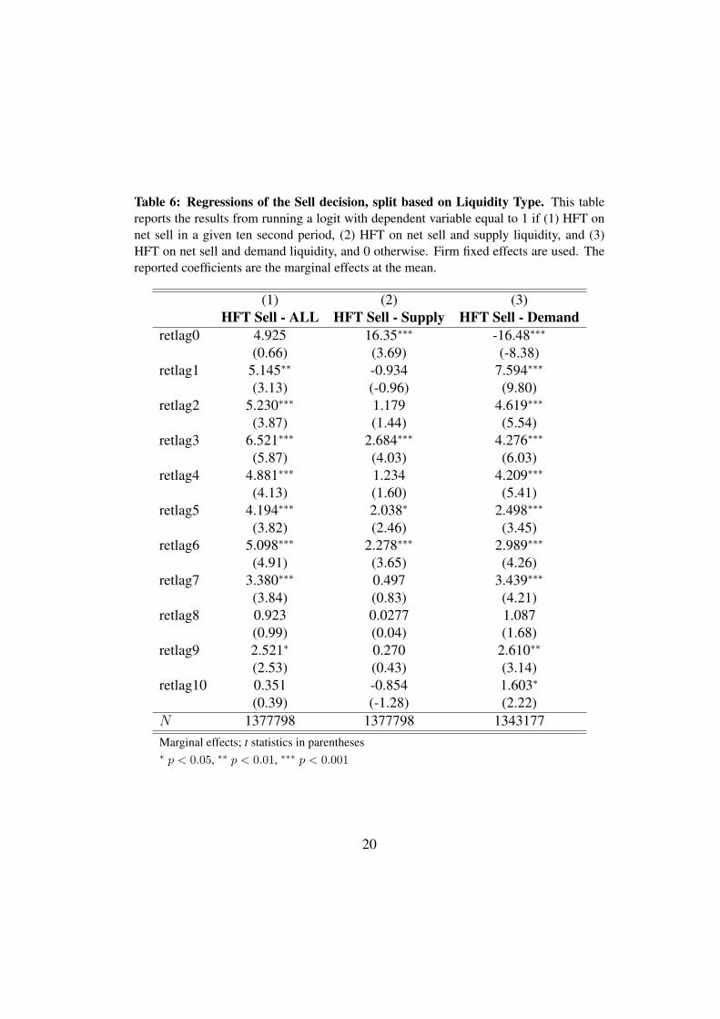
Table 6: Regressions of the Sell decision, split based on Liquidity Type. This tablereports the results from running a logit with dependent variable equal to 1 if (1) HFT onnet sell in a given ten second period, (2) HFT on net sell and supply liquidity, and (3)HFT on net sell and demand liquidity, and 0 otherwise. Firm fixed effects are used. Thereported coefficients are the marginal effects at the mean.

(1) (2) (3)HFT Sell - ALL HFT Sell - Supply HFT Sell - Demand

retlag0 4.925 16.35∗∗∗ -16.48∗∗∗

(0.66) (3.69) (-8.38)retlag1 5.145∗∗ -0.934 7.594∗∗∗

(3.13) (-0.96) (9.80)retlag2 5.230∗∗∗ 1.179 4.619∗∗∗

(3.87) (1.44) (5.54)retlag3 6.521∗∗∗ 2.684∗∗∗ 4.276∗∗∗

(5.87) (4.03) (6.03)retlag4 4.881∗∗∗ 1.234 4.209∗∗∗

(4.13) (1.60) (5.41)retlag5 4.194∗∗∗ 2.038∗ 2.498∗∗∗

(3.82) (2.46) (3.45)retlag6 5.098∗∗∗ 2.278∗∗∗ 2.989∗∗∗

(4.91) (3.65) (4.26)retlag7 3.380∗∗∗ 0.497 3.439∗∗∗

(3.84) (0.83) (4.21)retlag8 0.923 0.0277 1.087

(0.99) (0.04) (1.68)retlag9 2.521∗ 0.270 2.610∗∗

(2.53) (0.43) (3.14)retlag10 0.351 -0.854 1.603∗

(0.39) (-1.28) (2.22)N 1377798 1377798 1343177Marginal effects; t statistics in parentheses∗ p < 0.05, ∗∗ p < 0.01, ∗∗∗ p < 0.001

20

The last column in table 7 has as the dependent variable a one if HFT wereon net taking liquidity from the market and buying during the ten second intervaland a zero otherwise. There is still some statistical significance from the ten pastreturn periods, but only in time periods 0 and 3 - 6. The signs for the lag returnsare negative as expected, except for the contemporaneous period return, which islarge and positive. Like in the HFT Sell - Demand scenario, it is not clear fromthis logit model how to interpret this.

The results in table 6 and 7 show that HFT are engaged in a price reversalstrategy. This is true whether they are supplying liquidity or demanding it.

5.1.1 Front Running

A potential investing strategy of which HFT have been claimed to be engaged inis front running. That is, the anecdotal evidence charges HFT with detecting whenother market participants hope to move a large number of shares in a company andthat the HFT enters into the same position just before the other market participant.It is in this context where the HFT pinging, as defined in the Definitions section,and the SEC’s concern with it apply. That is, some claim HFT ping stock pricesto detect large orders being executed. If they detect a large order coming throughthey may increase their trading activity. The result of such an action by the HFTwould be to drive up the cost for the non-HFT market participant to execute thedesired transaction.

To see whether or not this is occurring on a systematic basis I perform thefollowing exercise: For each stock over the database time series I create twentybins based on trade size for trades initiated by non-HFT. Each bin has roughlythe same number of observations. Next, I look at the average percent of tradesthat were initiated by a HFT for different number of trades prior to the non-HFTinitiated trade (for prior trades 1 - 10).

I graph the results in figure 5. The x-axis is the 20 different non-HFT initiatedtrade size bins; the y-axis is the fraction of trades for different non-HFT trade sizebins for different prior trade periods that were initiated by a HFT; the z-axis is thedifferent prior trade periods.

The figure suggests front running by HFT before large orders is not systemati-cally occurring. In fact, it appears that larger trades, relative to each stock, tend tobe preceded by fewer HFT initiated trades. The non-HFT trades that are precededby the highest number of HFT initiated trades are those that are small and thoseare of moderate size. Also, it is interesting that the immediately preceding tradestend to have fewer HFT initiated trades than those further out. As will be shownlater, trades initiated by one type of market participant have a greater probability

21

Table 7: Regressions of the Buy decision, split based on Liquidity Type. This tablereports the results from running a logit with dependent variable equal to 1 if (1) HFT onnet buy in a given ten second period, (2) HFT on net buy and supply liquidity, and (3)HFT on net buy and demand liquidity, and 0 otherwise. Firm fixed effects are used. Thereported coefficients are the marginal effects at the mean.

(1) (2) (3)HFT Buy - ALL HFT Buy - Supply HFT Buy - Demand

retlag0 -2.793 -48.10∗∗∗ 53.48∗∗∗

(-0.37) (-14.21) (18.93)retlag1 -6.490∗∗∗ -4.910∗∗∗ -0.874

(-3.87) (-4.25) (-0.69)retlag2 -5.763∗∗∗ -4.533∗∗∗ -1.408

(-4.44) (-4.38) (-1.80)retlag3 -7.460∗∗∗ -4.257∗∗∗ -2.906∗∗

(-6.29) (-6.80) (-2.89)retlag4 -6.291∗∗∗ -2.802∗∗∗ -3.202∗∗∗

(-5.25) (-3.75) (-3.84)retlag5 -6.384∗∗∗ -2.572∗∗∗ -3.023∗∗∗

(-6.34) (-3.32) (-4.32)retlag6 -6.110∗∗∗ -3.042∗∗∗ -2.766∗∗∗

(-6.14) (-4.28) (-3.85)retlag7 -3.260∗∗ -2.001∗∗ -1.022

(-3.13) (-2.67) (-1.45)retlag8 -2.274∗ -1.553∗ -0.226

(-2.43) (-2.50) (-0.28)retlag9 -2.770∗∗ -1.513∗ -1.395∗

(-2.77) (-2.08) (-2.01)retlag10 -2.049∗ -1.908∗∗ 0.445

(-2.26) (-2.88) (0.67)N 1377798 1366278 1377798Marginal effects; t statistics in parentheses∗ p < 0.05, ∗∗ p < 0.01, ∗∗∗ p < 0.001

22

Figure 1: HFT Front Running. The graph shows the percent of trades initiated by HFTfor different prior time periods that precede different size non-HFT initiated trades. Thex-axis is the 20 different non-HFT initiated trade size bins; the y-axis is the fraction oftrades for different non-HFT trade size bins for different prior trade periods that wereinitiated by a HFT; the z-axis is the different prior trade periods.

23

of being preceded by the same type of market participant.

5.1.2 HFT Market Activity

In addition to understanding the trading behavior of HFT at the trade by tradelevel, it is informative to understand what drives HFT to trade in certain stockson certain days. Table 8 shows the variation in HFT market makeup in differentstock on different days. Panel A is the percent of trading variation of non-HFT andHFT in a certain stock on a given day. Panel B is the percent of trading variation ofHFT trading and non-HFT in supplying liquidity for a particular stock on a givenday. Panel C is the percent of trading variation of HFT trading and non-HFT indemanding liquidity for a particular stock on a given day.

Panel A shows that HFT’s share of the market varies a great deal depending onthe stock and the day. Its percent of all trades varies from 10.8% to 93.6% basedon number of trades. They average being involved in 61.8% of all trades, whichcompared to the numbers seen in the descriptive statistics from table 4, suggeststhat they trade more in stocks that trade frequently, as they make up 77% of alltrades in the entire market.

Panel B looks at HFT supplying liquidity. HFT supply liquidity in 35.5% oftrades in the average stock per day. This number is substantially smaller than the50% they were found to supply in the market as a whole in table 4. Thus, HFTmust supply liquidity in stocks that trade more frequently. Also, notice the widevariation in the supply of liquidity, in some stocks they provide no liquidity, whilein others they supply 74%.

Panel C looks at HFT demanding liquidity. They demand liquidity in 39.6% oftrades in the average stock per day. So HFT must be taking liquidity in stocks thattrade more frequently. Also, the HFT demand for liquidity varies substantiallyranging from 3.6% to 79.9%, but less than when they supply liquidity.

The results in table 8 show there is a large variation in the degree HFT tradingin different stocks over time, the next step is to consider which determinants resultin HFT increasing or decreasing their activity.

5.1.3 HFT Market Activity Determinants

Table 9 examines which determinants drive HFT trading. I perform an OLS re-gression, with the dependent variable being the percent of share volume, in whichHFT were involved in for a given company on a given day. I run the followingregression:

24

Table 8: Summary statistics 1 This table shows the variation in HFT market makeup.Panel A is the percent of trading variation of non-HFT and HFT in a certain stock on agiven day. Panel B is the percent of trading variation of HFT trading and non-HFT insupplying liquidity for a particular stock on a given day. Panel C is the percent of tradingvariation of HFT trading and non-HFT in demanding liquidity for a particular stock on agiven day.

Panel A - HFT Involved In A Stock

Trades SharesType of Trader Mean Median Std.

Dev.Min Max Mean Median Std.

Dev.Min Max

HFT 61.8% 64.0% 18.25 10.8% 93.6% 58.4% 59.4% 17.99 7.8% 90.9%Non HFT 39.3% 37.1% 19.24 6.4% 92.2% 42.7% 41.6% 18.83 9.1% 93.1%Total 100.0%100.0% 100.0%100.0%

Panel B - HFT Involved In A Stock As Liquidity Supplier

HFT 36.8% 35.5% 15.99 0% 74.4% 33.4% 32.7% 14.54 0.2% 66.4%Non HFT 64.1% 65.3% 16.63 25.6% 100.0%67.5% 67.9% 15.13 33.6% 100.0%Total 100.0%100.0% 100.0%100.0%

Panel C - HFT Involved In A Stock As Liquidity Taker

HFT 39.6% 40.3% 16.43 3.6% 79.9% 37.8% 37.7% 16.49 2.6% 78.9%Non HFT 61.1% 60.3% 16.70 20.1% 96.4% 62.8% 62.7% 16.73 21.1% 97.4%Total 100.0%100.0% 100.0%100.0%

25

Hi,t = α+MCi ∗ βi +MBi ∗ βi +NTi,t ∗ βi,t +NVi,t ∗ βi,t +Depi,t ∗ βi, t+ V oli,t ∗ βi,t + ACi,t ∗ βi, t,

where i is the subscript representing the firm, t is the subscript for each day, His the percent of share volume in which HFT are involved out of all trades, MC isthe log market capitalization as of December 31, 2009, MB is the market to bookratio as of December 31, 2009, which is winsorized at the 99th percentile, NT isthe number of non HFT trades that occurred, scaled by market capitalization, NVis the volume of non HFT dollars that were exchanged, scaled by market capital-ization, Dep is the average depth of the bid and of the ask, equally weighted, V olis the ten second realized volatility summed up over the day, AC is the absolutevalue of the Durbin-Watson score minus two from a regression of returns over thecurrent and previous ten second period.

Table 9 reports the standardized regression coefficients. That is, instead ofrunning the typical OLS regression on the regressors, the variables, both depen-dent and independent, are de-meaned, and are divided by their respective standarddeviations so as to standardize all variables. The coefficients reported can be un-derstood as signaling that when there is a one standard deviation change in anindependent variable, the coefficient is the expected change in standard deviationsthat will occur in the dependent variable. This makes the regressors underlyingscale of units irrelevant to interpreting the coefficients. Thus, the larger the coef-ficient, the more important its role in impacting the dependent variable.

The results show that market capitalization is very important and has a posi-tive relationship with HFT market percent. The market to book ratio is slightlystatistically significant, but with a very small negative coefficient, suggesting HFTtend to slightly prefer value firms. Also statistically significant and with moderateeconomically significant is the dollar volume of non HFT trading, which is inter-preted as HFT preferring to trade when there is less volume, all else being equal.The spread and depth variables are statistically significant and both have mediumeconomically significance. HFT prefer to trade when there is less depth and lowerspreads between bids and asks, all else being equal. Volatility, autocorrelation,and the number of non HFT trades are not statistically significant.

26

Table 9: Determinants of HFT Percent of the Market This table has as the dependentvariable the percent (in dollar volume) of trades involving a HFT for a given stock on agiven day.

(1)Economic Impact

Market Cap. 0.722∗∗∗

(19.51)Market / Book -0.063∗

(-2.13)$ of Non HFT Volume -0.138∗∗∗

(-3.82)Average Spread -0.111∗∗∗

(-3.88)Average Depth -0.132∗∗∗

(-4.79)Volatility -0.031

(-1.07)Autocorrelation -0.017

(-0.62)# of Non HFT Trades 0.042

(0.98)Constant ∗

(2.54)Observations 590Adjusted R2 0.575Standardized beta coefficients; t statistics in parentheses∗ p < 0.05, ∗∗ p < 0.01, ∗∗∗ p < 0.001

27

5.1.4 HFT Market Activity Time Series

A concern surrounding the May 6 “flash crash” was that the regular market par-ticipants, such as HFT, stopped trading. Although the database I have does notinclude the May 6, 2010 date, it does span 2008 and 2009, which were volatiletimes in U.S. equity markets. To see whether HFT percent of market trades variessignificantly from day to day, and especially around time periods when the U.S.market experienced large losses, I look at each trading day and count what frac-tion of trades in which HFT were involved. The results are shown in figure 2.There are three graphs. The first is a time series of the fraction of trades HFTwere involved in during 2008 and 2009. The second graph looks at the fraction ofshares in which HFT were involved during this period. The final graph looks atthe fraction of dollar volume in which HFT were involved during this period. Ineach graph there are three lines. The line labeled “All HFT” represents the frac-tion of exchanges in which HFT were involved either as a liquidity provider or aliquidity taker; the line labeled “HFT Liquidity Supplied” represents the fractionof transactions in which HFT were providing liquidity; the line “HFT LiquidityDemanded” represents the fraction of trades in which HFT were demanding liq-uidity. All three graphs have minimal volatility among the three measures. Espe-cially of note, there is no abnormally large drop, or increase, in HFT participationoccurring in September of 2009, when the U.S. equity markets were especiallyvolatile.

5.2 Profitability

HFT engage in a price reversal strategy and they make up a large portion of themarket. Given their trading amount a question of interest is how profitable is theirbehavior. HFT have been portrayed as making tens of billions of dollars fromother investors. Due to the limitations of the data, I can only provide an estimateof the profitability of HFT. The HFT labeled trades come from many firms, but Icannot distinguish which HFT firm is buying and selling at a given time. Also,recall the dataset only contains Nasdaq trades. Therefore, there will be many othertrades that occur that the dataset does not include. Nasdaq makes up about 20%of all trades and so 4 out of every 5 trades are not part of the data set.

I consider all HFT to be one trader. I take all the buys and sells at the respec-tive prices of the HFT and calculate how much money was spent on purchasesand received from sales. HFT tend to switch between being net long and net shortthroughout the day, but at the end of the day they tend to hold very few shares.With these considerations in mind, I can calculate an estimate of the total prof-

28

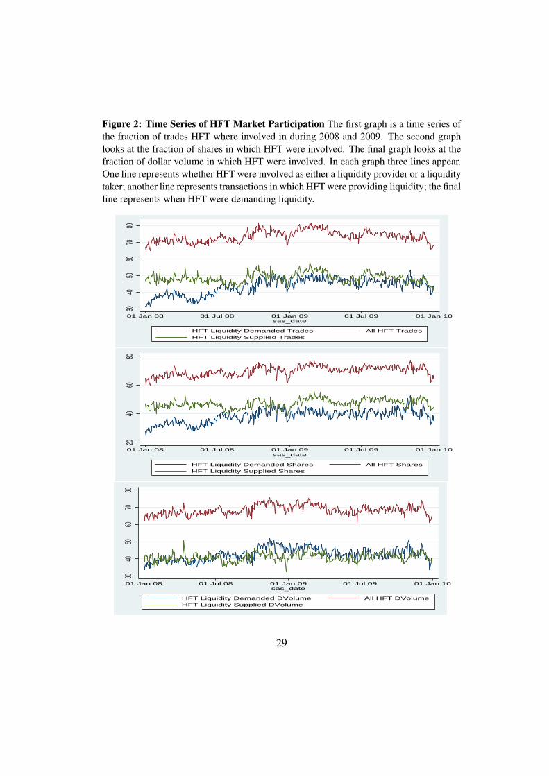
Figure 2: Time Series of HFT Market Participation The first graph is a time series ofthe fraction of trades HFT where involved in during 2008 and 2009. The second graphlooks at the fraction of shares in which HFT were involved. The final graph looks at thefraction of dollar volume in which HFT were involved. In each graph three lines appear.One line represents whether HFT were involved as either a liquidity provider or a liquiditytaker; another line represents transactions in which HFT were providing liquidity; the finalline represents when HFT were demanding liquidity.

3040

5060

7080

01 Jan 08 01 Jul 08 01 Jan 09 01 Jul 09 01 Jan 10sas_date

HFT Liquidity Demanded Trades All HFT TradesHFT Liquidity Supplied Trades

2040

6080

01 Jan 08 01 Jul 08 01 Jan 09 01 Jul 09 01 Jan 10sas_date

HFT Liquidity Demanded Shares All HFT SharesHFT Liquidity Supplied Shares

3040

5060

7080

01 Jan 08 01 Jul 08 01 Jan 09 01 Jul 09 01 Jan 10sas_date

HFT Liquidity Demanded DVolume All HFT DVolumeHFT Liquidity Supplied DVolume

29

itability of these 26 firms. As many stocks do not end the day with an exact netzero buying and selling by HFT, I take any excess shares and assume they weretraded at the mean price of that stock for that day. The result of this exercise isthat on average, per day, HFT make $298,113.1 from the 120 stocks in my sampleon trades that occur on Nasdaq.

The above number substantially underestimates the actual profitability of HFT.First, the 120 stocks have a combined market capitalization of $2,110,589.3 (mil-lion), whereas all compustat firms’ combined market capitalization is $17,156,917.3(million), and so I should multiply the profitability by 8.13, raising the per dayHFT profitability from all stocks to $2,423,659.5 per day. The other large factorto be incorporated is that Nasdaq trades make up approximately 20% of all trades,so assuming HFT trade on other exchanges as they do on Nasdaq, the previousnumber should be multiplied by five. Thus the estimated daily profit of these 26firms is $12,118,297.5. Per year that is $3,029,574,380. Although this is a largeabsolute number, relatively it is small, especially given that HFT trade around $30trillion annually.

There is no adjustment made for transaction costs yet. However, such costswill be negligible, the reason being that when HFT provide liquidity they receivea rebate from the exchange, for example Nasdaq offers $.20 per 100 shares forwhich traders provided liquidity, but this is only for large volume traders like theHFT. On the other hand, Nasdaq charges something like $.25 per 100 shares forwhich trades take liquidity. As the amount of liquidity demanded is slightly lessthan the liquidity supplied by HFT, these two values practically cancel themselvesout.

Figure 3 displays the time series of HFT profitability per day. The graph is afive day-moving average of profitability of HFT per day for the 120 firms in thedataset. Profitability varies substantially from day to day, even after smoothingout the day to day fluctuations.

To try to understand what drives the changes in profitability per day I lookat the determinants for what stocks on different days are the most profitable. Iregress the profitability on several potentially important variables, the same onesused in the regression to determine HFT percent of the market. I run the followingstandardized regression (to obtain the economic impact):

Profiti,t = α+Hi,t ∗ βi,t +MCi ∗ βi +MBi ∗ βi +NTi,t ∗ βi,t +NVi,t ∗ βi,t +Depi,t ∗ βi, t+ V oli,t ∗ βi,t + ACi,t ∗ βi, t,

30

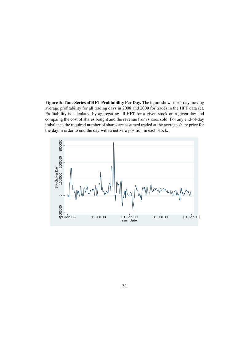
Figure 3: Time Series of HFT Profitability Per Day. The figure shows the 5-day movingaverage profitability for all trading days in 2008 and 2009 for trades in the HFT data set.Profitability is calculated by aggregating all HFT for a given stock on a given day andcompaing the cost of shares bought and the revenue from shares sold. For any end-of-dayimbalance the required number of shares are assumed traded at the average share price forthe day in order to end the day with a net zero position in each stock.

−100

0000

010

0000

020

0000

030

0000

0$

Prof

it Pe

r Day

01 Jan 08 01 Jul 08 01 Jan 09 01 Jul 09 01 Jan 10sas_date

31

where all variables are defined as before, and the dependent variable Profittakes on three different definitions. The results are displayed in Table 10. In thefirst column Profit is defined as the profit per HFT share traded averaged overstock i on day t; in the second column it is the amount of money HFT madefor stock i on day t; in the third column it is the number of HFT shares tradedfor stock i on day t. The second and third regression decompose the parts ofthe first regression’s dependent variable. Again, the reported coefficients havebeen standardized so that the coefficient value represents a one standard deviationmovement in a particular variable’s impact on Profit.

The Profit per HFT Share Traded regression has no statistically or economi-cally significant variables and has a negative r-squared. The second regression,with the dependent variable as profits, has two coefficients that are statisticallysignificant. Autocorrelation and Volatility. Autocorrelation has a smaller coeffi-cient and is negative, implying the less predictable price movements in a stock themore profitable is that stock for HFT. The V olatility measure has a large positiveeconomic impact and is highly statistically significant.

The third regression, HFT shares traded, has three statistically significant andeconomically significant variables. MarketCap. is positive with a coefficient of0.21, the AverageDepth coefficient is positive and has a coefficient of 0.098,and the V olatility coefficient, which also has a positive relationship with thedependent variable, shows the largest coefficient magnitude of 0.622.

The results in this section have shown that HFT engage in a price reversaltrading strategy, that HFT tend to trade more in large stocks with relatively lowvolume with narrow spreads and depth. Also, HFT are profitable, making approx-imately $3 billion a year, and that the profitability is driven by volatility. Next, Iinvestigate the role HFT play in demanding and supplying liquidity.

6 Market QualityThe following section analyzes HFT impact on market quality. Market qualityrefers to liquidity, price discovery, and volatility. Each analysis uses differenttechniques to study the relationship between HFT and each type of market quality.

6.1 HFT Liquidity

Liquidity supply and demand in the microstructure literature refers to which sideof the transaction entered the marketable order and which side had a limit orderin place that was executed. The side with the limit order is the liquidity supplier,and the marketable order side is the liquidity taker. In this section I look at the de-

32

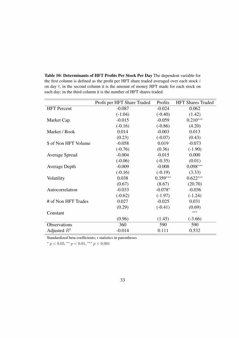
Table 10: Determinants of HFT Profits Per Stock Per Day The dependent variable forthe first column is defined as the profit per HFT share traded averaged over each stock ion day t; in the second column it is the amount of money HFT made for each stock oneach day; in the third column it is the number of HFT shares traded.

Profit per HFT Share Traded Profits HFT Shares TradedHFT Percent -0.087 -0.024 0.062

(-1.04) (-0.40) (1.42)Market Cap. -0.015 -0.059 0.210∗∗∗

(-0.16) (-0.86) (4.20)Market / Book 0.014 -0.003 0.013

(0.23) (-0.07) (0.43)$ of Non HFT Volume -0.058 0.019 -0.073

(-0.76) (0.36) (-1.90)Average Spread -0.004 -0.015 0.000

(-0.06) (-0.35) (0.01)Average Depth -0.009 -0.008 0.098∗∗∗

(-0.16) (-0.19) (3.33)Volatility 0.038 0.359∗∗∗ 0.622∗∗∗

(0.67) (8.67) (20.70)Autocorrelation -0.033 -0.078∗ -0.036

(-0.62) (-1.97) (-1.24)# of Non HFT Trades 0.027 -0.025 0.031

(0.29) (-0.41) (0.69)Constant ∗∗∗

(0.96) (1.45) (-3.66)Observations 360 590 590Adjusted R2 -0.014 0.111 0.532Standardized beta coefficients; t statistics in parentheses∗ p < 0.05, ∗∗ p < 0.01, ∗∗∗ p < 0.001

33

scriptive statistics of how HFT demand liquidity, then I examine how they supplyliquidity, finally I analyze how much liquidity they provide in the quotes and thebook, not just for trades.

6.1.1 HFT Liquidity Demand

The results in table 4 show that liquidity is demanded by HFT in 50.4% of alltrades. This section will analyze how HFT initiated trades tend to behave com-pared to non-HFT trades. HFT tend to demand liquidity in similar dollar sizetrades as do non HFT. There appears to be clustering in trades, whereby if a previ-ous trade is a buy, it is much more likely the next trade will also be a buy, and thesame is true for sales, and this clustering is stronger for HFT than for Non-HFT.Trades that either proceed a HFT or follow a HFT tend to occur more quicklythan those proceeding or following a non-HFT. As trade size increases, the timebetween trade decreases, and this is true regardless of the size of the firm. Finally,HFT demands are quite consistent across the day, but they make up a significantlysmaller portion of trades at the opening and close of the trading day.

Table 11 looks at the percent of all transactions for different size trades, indollar terms, and with different HFT and non-HFT liquidity providers and de-manders. The first column of Table 11 reports the fraction of trading volume fordifferent combinations of HFT firms and non-HFT firms as liquidity providersand takers. For small trades, those worth less than $1,000 HFT are not as involvedas Non HFT, this is consistent with the previous results that show HFT tended totrade more in stocks with large market caps, which typically have stock prices inthe double digits. Most trades occur in the value range of $1,000 to $4,999. TheHFT in two of their three categories are the most engaged in these transactions.HFT’s share of trades engaged in falls in the $5,000 to $14,999 category, exceptfor when they are demanding liquidity. In the $30,000 plus category of trades,HFT provide the least amount of liquidity, but tend to demand the most. This sug-gest that HFT are liquidity takers in large trades and liquidity providers in smallshares, which is consistent with the theory that HFT are concerned with informedtraders in big trades.

The previous table analyzed the frequency of different types of trades, thenext table examines the conditional frequency and occurrence of different types oftrades. Table 12, similar to that in Biais, Hillion, and Spatt (1995) and Hendershottand Riordan (2009), provides evidence on the clustering of HFT trades in tradesequences. In the table, H stands for HFT and N stands for non-HFT. The firstletter in the rows for Panel A and B is who is demanding liquidity at Time t-1. The second letter in these two panels is who is demanding liquidity at time

34

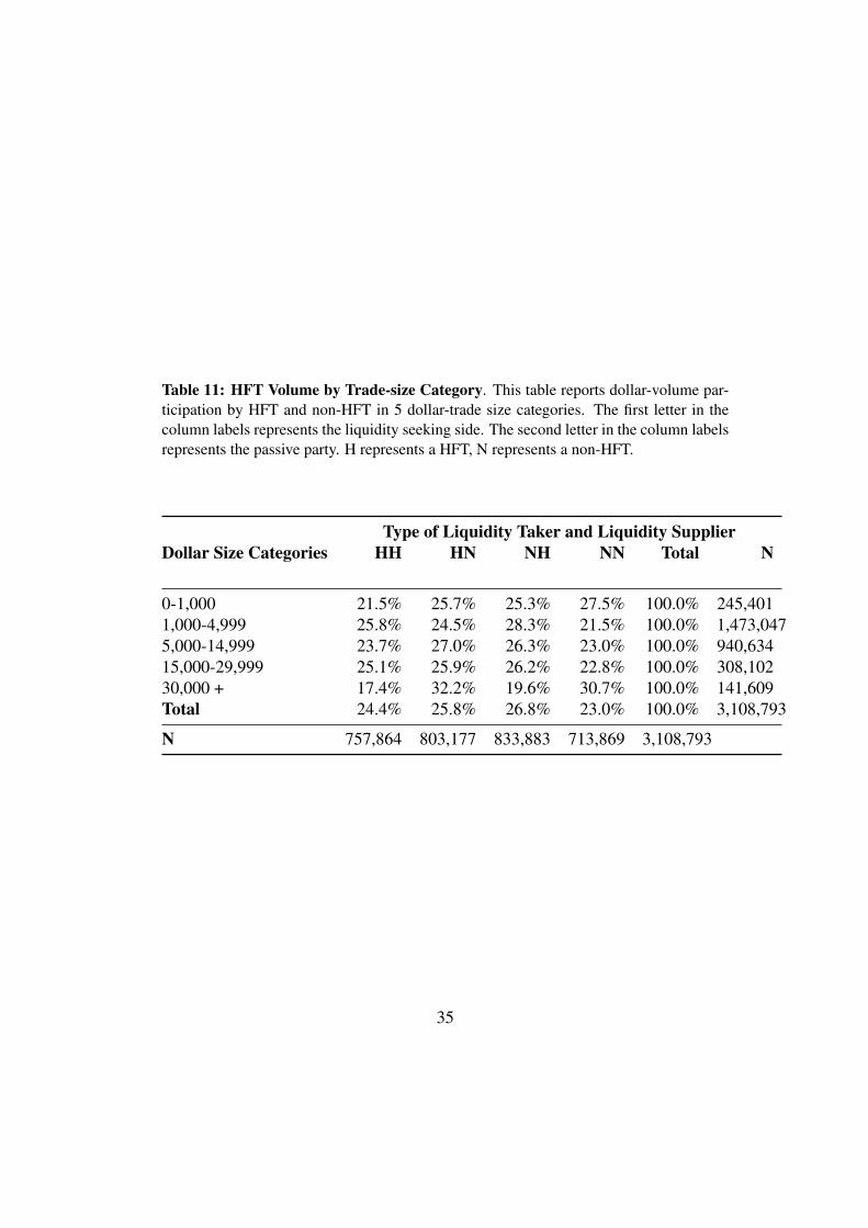
Table 11: HFT Volume by Trade-size Category. This table reports dollar-volume par-ticipation by HFT and non-HFT in 5 dollar-trade size categories. The first letter in thecolumn labels represents the liquidity seeking side. The second letter in the column labelsrepresents the passive party. H represents a HFT, N represents a non-HFT.

Type of Liquidity Taker and Liquidity SupplierDollar Size Categories HH HN NH NN Total N

0-1,000 21.5% 25.7% 25.3% 27.5% 100.0% 245,4011,000-4,999 25.8% 24.5% 28.3% 21.5% 100.0% 1,473,0475,000-14,999 23.7% 27.0% 26.3% 23.0% 100.0% 940,63415,000-29,999 25.1% 25.9% 26.2% 22.8% 100.0% 308,10230,000 + 17.4% 32.2% 19.6% 30.7% 100.0% 141,609Total 24.4% 25.8% 26.8% 23.0% 100.0% 3,108,793

N 757,864 803,177 833,883 713,869 3,108,793

35

t. Panel A reports the unconditional frequency of observing HFT and non-HFTtrades. Seeing a HFT demand liquidity in time t-1 followed by a HFT demandingliquidity in time t is as common as seeing any other time t-1, t sequence. PanelB reports the conditional frequency of observing HFT and non-HFT trades afterobserving trades of other participants. In Panel B, the columns are whether theliquidity taker is buying (B) or selling (S). The first letter represents what theliquidity taker is doing in the time t-1 trade. The second letter represents what theliquidity taker is doing in the time t trade. In column and row headings t indexestrades, not time. The results suggest that one tends to see liquidity demanderspurchase shares follow a previous trade of a liquidity demander purchasing shares,and the same with sales, regardless of what type of trader was demanding theliquidity. The clustering affect is stronger, in both buying and selling, for HFTdemanders than it is for Non-HFT demanders.

Panel C provides conditional probabilities based on the previous trade’s sizeand type of trader. The rows represent the type of trader taking liquidity at time t-1, either H for HFT or N for non-HFT. In addition, the rows are further partitionedbased on the size of the trade, measured by the dollar size of shares exchanged inthe t-1 trade. 1 represents a trade of size $0 -$999; 2 represents a trade of size$1,000 - $4,999; 3 represents a trade of size $5,000 - $14,999; 4 represents a tradeof size $15,000 - $29,999; and 5 represents a trade of size greater than $30,000.The columns identify who was the liquidity demander at time t (H or N) and isfurther partitioned along the size categories discussed above. The results showthat trades of size and type of liquidity demander are highly dependent on theprevious trade type. HFT tend to trade with HFT, and the larger the dollar size ofa trade the higher the likelihood the next trade will be large.

The next set of results regarding type of trader initiating trading looks at thetime between trades. Table 13 reports the average time between trades depen-dent on different trade characteristics. All times reported are in seconds. PanelA reports the average amount of time between two trades, two HFT liquidity de-manding trades, and two non-HFT liquidity demanding trades, and between atrade where the t-1 trade was initiated by a trader who was a HFT, or a non-HFT.Both trades when the liquidity demander is HFT at both t-1 and t, and when HFTis the liquidity demander at t-1, regardless of who demands liquidity at time t, aremore rapidly executed.

Panel B provides the average amount of time between two different trade or-derings and total dollar-volume and per trade dollar-volume categories. The firsttwo columns in Panel B is for some trade type at t-1 and at time t there is a liquid-ity taker of H or N, where the columns are separated based on the time t liquidity

36

Table 12: Trade Frequency Conditional on Previous Trade. Panel A reports the un-conditional frequency of observing HFT and non-HFT trades. Panel B reports the con-ditional frequency of observing HFT and non-HFT trades after observing trades of otherparticipants. In column and row headings t index trades. Panel C provides conditionalprobabilities based on the previous trade’s size and participant. The first letter in the rowsfor Panel A and B is who is demanding liquidity at Time t-1. The second letter in thesetwo panels is who is demanding liquidity at time t.

Panel A

T-1 Type and T Type %

HH 24.4%HN 25.8%NH 26.8%NN 23.0%Total 100.0%

Panel B

T-1 Buy or Sell and T Buy or SellT-1 Type and T Type BB BS SB SS Total

% % % % %

HH 44.3% 5.9% 5.9% 43.9% 100.0%HN 44.1% 6.5% 6.3% 43.1% 100.0%NH 41.9% 7.5% 7.7% 42.9% 100.0%NN 41.5% 7.7% 7.8% 42.9% 100.0%Total 43.0% 6.9% 6.9% 43.2% 100.0%

Panel C

LD Sizelag LD Size H1 H2 H3 H4 H5 N1 N2 N3 N4 N5 Total

% % % % % % % % % % %

H1 25.9% 32.2% 13.3% 2.5% 1.0% 7.5% 10.8% 5.4% 0.8% 0.4% 100.0%H2 5.1% 58.2% 14.8% 3.8% 1.6% 1.3% 11.4% 3.0% 0.7% 0.3% 100.0%H3 3.2% 23.1% 46.2% 6.1% 2.3% 0.9% 4.3% 12.0% 1.3% 0.5% 100.0%H4 1.9% 18.2% 18.7% 35.0% 7.6% 0.5% 2.9% 4.5% 8.6% 2.1% 100.0%H5 1.7% 17.0% 16.2% 17.3% 27.8% 0.5% 2.7% 3.9% 5.2% 7.6% 100.0%N1 6.8% 7.4% 3.5% 0.7% 0.3% 39.6% 29.5% 9.6% 1.7% 0.8% 100.0%N2 1.7% 11.5% 2.8% 0.7% 0.3% 5.3% 57.9% 14.5% 3.6% 1.8% 100.0%N3 1.3% 4.6% 12.4% 1.6% 0.6% 2.7% 23.1% 44.8% 6.0% 2.7% 100.0%N4 0.6% 3.4% 3.9% 9.0% 2.5% 1.5% 17.8% 18.6% 34.5% 8.1% 100.0%N5 0.7% 3.7% 4.0% 4.8% 7.9% 1.5% 18.3% 18.0% 17.3% 23.9% 100.0%Total 3.7% 23.9% 15.4% 5.1% 2.3% 4.2% 23.6% 14.9% 4.8% 2.2% 100.0%

37

taker. The last two columns is similar except that its columns are distinguishedbased on the time it takes when the time t-1 liquidity taker is a certain type (H orN). Rows S1 through M5 represent different types of stocks. The first character,S,M, or L, represents the dollar volume traded in a given stock on a given day, withS being for trades in small stocks with total dollar volume under $800 Million, Mfor medium stocks with dollar volume between $800 Million and $1.2 Billion,and L for large stocks with dollar volume greater than $1.2 Billion. The secondcharacter ,the number 1 through 5 represents the size of the particular trade. Ifthe trade was less than $1000 then it is a 1, if its between $1,000 and $4,999 itsa 2, if between $5,000 and $14,999 its a 3, if between $15,000 and $29,999 its a4, and if its greater than $30,000 it is a 5. The results suggest that as more dollarvolume is traded ,the time between trades decreases. Also, within each day dollarvolume category, the larger the trade, usually the shorter the time before anothertrade occurs. This is the opposite of what Hendershott and Riordan (2009) find;they see that small orders for Algorithmic Traders tend to execute faster. This isevidence that HFT actively monitor the market for liquidity, but that they focustheir trading strategy around price pressures from large trades. Finally, for mostof the different categories, HFT tend to trade more rapidly, whether looking attime t-1 or time t.

Finally, I examine the intraday pattern of HFT supply and demand of liquidity.If HFT do try and end the day with a near net zero position in stocks then theyshould wind down their trading before the end of the trading day in order to pre-vent getting stuck with shares in their position they do not want to hold overnight.Similarly, at the beginning of the trading day they will have few positions in whichthey are trying to maintain a near net zero position in and so trading should be lessprevalent. To analyze this I create a time series of the type of traders throughoutthe day. I take all trades that occur on February 22, 2010 - February 26, 2010 andput them in to ten second bins based on the time of day they occurred, regardlessof the day. Then, I split them into the types of trades based on who was supplyingliquidity and demanding liquidity and calculate the percent of each type of trans-action per time period bin. Figure 4 shows the make up of different types of tradesthroughout the day. The four different patterns, HH, HN, NH, NN refer to the typeof liquidity demander (first letter) and liquidity supplier (second letter). The figureis stacked so that each time period sums to one. During the day the trading ratiosare quite stable, except at the beginning and end of day. During these periods HFTtend to trade with each other much less frequently and HFT tend to initiate fewertrades and to provide liquidity in fewer trades. This is consistent with the scenarioof HFT trying to end the day near net-zero in their equity positions.

38

Table 13: Average Time Between Trades. All values are in seconds. Panel A reportsthe average amount of time between two trades, two HFT liquidity demanding trades,and two non-HFT liquidity demanding trades, and between a trade where the initial tradehad a HFT, or a non-HFT liquidity demander. Panel B provides the average amount oftime between two different trade orderings and trade-size categories (refer to the previoustable for the different trade-size categories) The first two columns in Panel B is for sometrade type at t-1 and at time t there is a liquidity taker of H or N, where the columns areseparated based on the time t liquidity taker. The last two columns is similar except thatits columns are distinguished based on the time it takes when the time t-1 liquidity takeris a certain type (H or N).

Panel AHFT Non-HFT

Unconditional Time Between Trades 3.351 5.667Time Between Trades of Same Type of Trader 8.696 9.081

Panel BTime t Liquidity Taker Time t-1 Liquidity TakerHFT Non-HFT HFT Non-HFT

S1 30.746 25.449 18.384 35.843S2 9.620 10.578 7.582 12.657S3 5.069 5.513 4.485 6.134S4 3.426 3.354 2.742 4.067S5 4.576 4.065 3.572 5.056M1 0.988 1.538 1.183 1.378M2 1.219 1.399 1.064 1.572M3 1.095 1.435 1.112 1.434M4 1.098 1.166 0.998 1.273M5 1.136 0.989 0.851 1.290L1 0.746 1.266 0.899 1.118L2 1.135 1.119 0.841 1.447L3 0.746 1.149 0.842 1.065L4 0.780 0.724 0.668 0.833L5 0.729 0.639 0.602 0.760

39

Figure 5 also looks at trades throughout the day, but only charts the percent ofdollar volume in which HFT are demanding liquidity (top graph) and supplyingliquidity (bottom graph). Again this shows that HFT significantly reduce boththeir supply and their demand for liquidity at the start and end of trading hours.

Figure 4: Type of Liquidity Providers / Takers throughout the day. The figure showsthe make up of traders throughout the day. It shows that HFT tend to reduce their tradingactivity at the opening and closing of the trading day. the first letter is the liquidity taker,the second letter is the liquidity provider.

.2.4

.6.8

1St

acke

d Pe

rcen

t of T

rade

s

9:43 11:6 12:30 1:53 3:16 4:40Time of Day

HH Transaction HN TransactionNH Transaction NN Transaction

6.1.2 HFT Liquidity Supply

This section analyzes how HFT supply liquidity. I focus on the amount of liquid-ity HFT supply. I show that, beyond supplying liquidity in 51.4% of all trades,they also often supply the inside quotes throughout the day. I then consider thedeterminants that determine which stocks, and on what days, do HFT providethe inside quotes. Finally, I examine what the additional price impact would beon stocks if HFT where not part of the book. There is a sizeable impact, whichshows the importance of HFT providing liquid markets.

6.1.2.1 HFT Time at Inside Quotes To begin analyzing HFT’s role in pro-viding liquidity in the stock market I look at the amount of time HFT supply theinside bid or ask compared to non-HFT firms. For each stock, on each day, I take

40

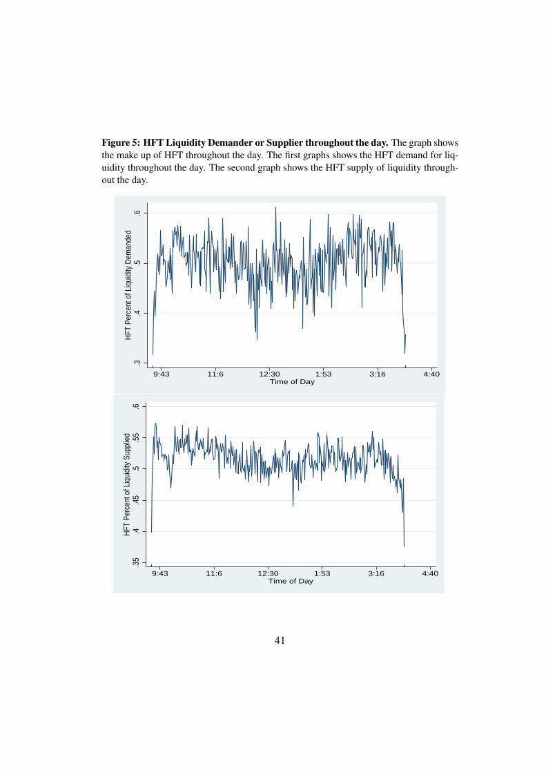
Figure 5: HFT Liquidity Demander or Supplier throughout the day. The graph showsthe make up of HFT throughout the day. The first graphs shows the HFT demand for liq-uidity throughout the day. The second graph shows the HFT supply of liquidity through-out the day.

.3.4

.5.6

HFT

Per

cent

of L

iqui

dity

Dem

ande

d

9:43 11:6 12:30 1:53 3:16 4:40Time of Day

.35

.4.4

5.5

.55

.6H

FT P

erce

nt o

f Liq

uidi

ty S

uppl

ied

9:43 11:6 12:30 1:53 3:16 4:40Time of Day

41

the number of minutes HFT are providing the inside bid or ask and, either: (a)subtract the number of minutes non-HFT are providing the best inside bid or ask(ties are dropped), these are the “Minutes” results, or (b), divide this value by thetotal number of minutes where HFT and non-HFT did not have the same insidequotes, these are the “Percent” results. The results are in Table 14.

Table 14 looks at, for the 120 stocks, whether the HFT provide more liquiditythan non-HFT traders by considering how often they are providing the inside quote(bid or ask). The way the metric is constructed there are a total of 900 minutes( 2*60*7.5) that a HFT could potentially be providing the inside quote. This istwice as many minutes then what actually occur during the trading day. The tableis separated into two categories - the category “HFT -” is when the HFT providesfewer inside quotes than the non-HFT for a stock on a given day; category “HFT+” is when the HFT is more frequently the inside quote provider for a stock ona given day. The reason to separate out the two types is that it may be that somestocks HFT do not actively try and provide inside quotes for, thus just taking theaverage across all stocks would underweight the liquidity they provide in stocksfor which they are activily trying to place competitive quotes. Table 14 has threepanels, and within each panel either a category called “Minutes” or “Percent.”Panel A considers quotes for all stocks; Panel B considers quotes for stocks ondays they are below their average spread; and Panel C considers quotes for stockson days they are above their average spread. The Minutes results display thenumber of minutes HFT provide the inside quotes more than non-HFT throughthe following calculation: sum the number of minutes HFT provide the best bidor ask, subtract the number of minutes non-HFT are providing the best inside bidor ask, and drop ties. A problem with this is that since the ties will vary acrossdays and stocks, the Minutes approach does not necessarily capture the frequencythat HFT provide better inside quotes than non-HFT. The Percent results avoidsthis issue by dividing the number of minutes HFT provide the best quotes by thetotal number of minutes where HFT and non-HFT did not have the same insidequotes.

It does not appear there is a significant difference between the stocks in whichHFT decide to place aggressive bid/ask orders and those in which it does not.The very low value for the mean of Net - by itself may imply that the HFT do notattempt to match or out-price the quotes of non-HFT for some stocks. But lookingat the “Percent” data, shows that the Net - and Net + results are about equallydistant from .5. Thus, the “Minutes” Net - results must be biased downwards asa result of a large number of periods where HFT and non-HFT provide the sameprices. Looking at the Panel A - Percent results, on average HFT provide the

42

best inside quotes 45% of the time, a significant portion of the trading day. Thissuggests that HFT act as market makers and are competitive.

Panel B and C divide the stocks into those that are offering higher spreadsthan usual and those offering lower spreads than usual. Panel B reports the lowspread stock days, Panel C the high spread stock days. The results between thetwo subsets do not differ much from one another. The average time HFT offerthe best quotes is slightly higher when spreads are high at 71.7% compared to70.1% when it is low. Also, HFT provide the best quotes more often than non-HFT slightly more often when spreads are high, doing so 46% of the time asopposed to 45.1% when spreads are low. This is consistent with HFT attemptingto capture liquidity supply profits as found in Foucault and Menkveld (2008) andHendershott and Riordan (2009) make/take liquidity cycle, but as the differenceis small does not provide much support for it.

6.1.2.2 HFT Time at Inside Quotes Determinants Tables 14 shows that HFTare at the inside quotes frequently, but not as much as non-HFT. I perform an OLSregression similar to that found in table 9 to understand what determinants arerelated to which stocks and days HFT decide to provide the best quotes. Table 15shows the results. It is very similar to table 9, with all variables being definedexactly the same as before except the dependent variable. The regression is:

Li,t = α+MCi ∗ βi +MBi ∗ βi +NTi,t ∗ βi,t +NVi,t ∗ βi,t +Depi,t ∗ βi,t + V oli,t ∗ βi,t + ACi,t ∗ βi,t,

where the variables and subscripts are defined as above, and the dependentvariable, Li,t is the percent of the time for which HFT provide the best insidequotes compared to all times when HFT and non-HFT quotes differ.

The coefficients reported, like those in table 9, are standardized beta coeffi-cients which allows for an easy way to decide which determinants are more impor-tant. The results suggest there are several explanatory variables that matter, all ex-cept Autocorrelation are statistically significant, and all except AverageDepthhave coefficient magnitudes greater than .16. MarketCap. and #ofNonHFTTradeshave positive coefficients, with MarketCap. being the most important determi-nant of determining HFT providing the best quotes. The other coefficients arenegative, suggesting that HFT prefer to provide the inside quotes for value firms,less volatility firms, firms with narrower spreads, and firms with a lower bookdepth.

43

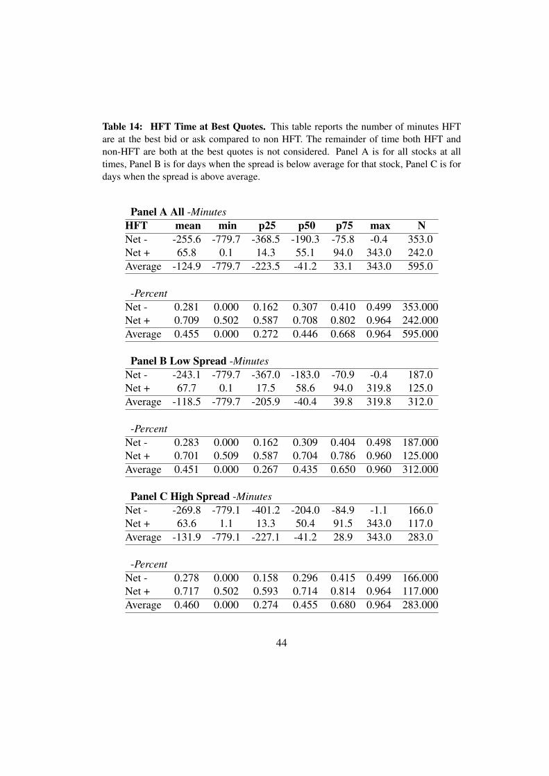
Table 14: HFT Time at Best Quotes. This table reports the number of minutes HFTare at the best bid or ask compared to non HFT. The remainder of time both HFT andnon-HFT are both at the best quotes is not considered. Panel A is for all stocks at alltimes, Panel B is for days when the spread is below average for that stock, Panel C is fordays when the spread is above average.

Panel A All -MinutesHFT mean min p25 p50 p75 max NNet - -255.6 -779.7 -368.5 -190.3 -75.8 -0.4 353.0Net + 65.8 0.1 14.3 55.1 94.0 343.0 242.0Average -124.9 -779.7 -223.5 -41.2 33.1 343.0 595.0

-PercentNet - 0.281 0.000 0.162 0.307 0.410 0.499 353.000Net + 0.709 0.502 0.587 0.708 0.802 0.964 242.000Average 0.455 0.000 0.272 0.446 0.668 0.964 595.000

Panel B Low Spread -MinutesNet - -243.1 -779.7 -367.0 -183.0 -70.9 -0.4 187.0Net + 67.7 0.1 17.5 58.6 94.0 319.8 125.0Average -118.5 -779.7 -205.9 -40.4 39.8 319.8 312.0

-PercentNet - 0.283 0.000 0.162 0.309 0.404 0.498 187.000Net + 0.701 0.509 0.587 0.704 0.786 0.960 125.000Average 0.451 0.000 0.267 0.435 0.650 0.960 312.000

Panel C High Spread -MinutesNet - -269.8 -779.1 -401.2 -204.0 -84.9 -1.1 166.0Net + 63.6 1.1 13.3 50.4 91.5 343.0 117.0Average -131.9 -779.1 -227.1 -41.2 28.9 343.0 283.0

-PercentNet - 0.278 0.000 0.158 0.296 0.415 0.499 166.000Net + 0.717 0.502 0.593 0.714 0.814 0.964 117.000Average 0.460 0.000 0.274 0.455 0.680 0.964 283.000

44

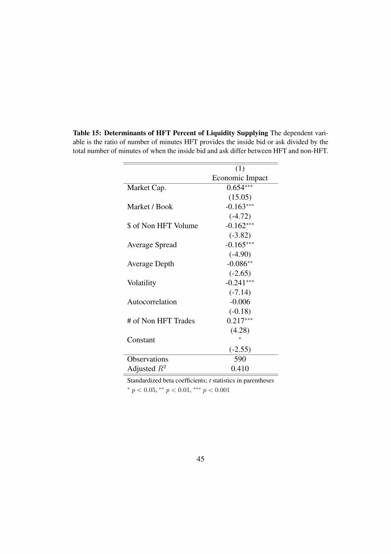
Table 15: Determinants of HFT Percent of Liquidity Supplying The dependent vari-able is the ratio of number of minutes HFT provides the inside bid or ask divided by thetotal number of minutes of when the inside bid and ask differ between HFT and non-HFT.

(1)Economic Impact

Market Cap. 0.654∗∗∗

(15.05)Market / Book -0.163∗∗∗

(-4.72)$ of Non HFT Volume -0.162∗∗∗

(-3.82)Average Spread -0.165∗∗∗

(-4.90)Average Depth -0.086∗∗

(-2.65)Volatility -0.241∗∗∗

(-7.14)Autocorrelation -0.006

(-0.18)# of Non HFT Trades 0.217∗∗∗

(4.28)Constant ∗

(-2.55)Observations 590Adjusted R2 0.410Standardized beta coefficients; t statistics in parentheses∗ p < 0.05, ∗∗ p < 0.01, ∗∗∗ p < 0.001

45

6.1.2.3 Price Impact Reduction from HFT Liquidity Thus far, the analysison liquidity has been by looking at the best inside bid and ask. Another way oflooking at HFT impact on liquidity is by looking at the depth of the book sup-plied by HFT. I analyze what difference having HFT providing liquidity in thebook provides in decreasing the price impact of a trade. That is, one can observethe book with all of the limit orders in it and then remove the liquidity providedby HFT and see what the impact would be on the cost of executing a trade fordifferent size trades. The results of this exercise are presented in Table 16. I con-sider a variety of different impacts based on the number of shares hypotheticallybought. The number of shares varies from 100 to 1000. I show the price impactbased on market capitalization and also for the overall sample (column All). Themarket capitalizations are divided so that Very Small includes firms under $ 400million, Small are those between $400 million and $1.5 billion, Medium are thosebetween $1.5 billion and $3 billion, and large are for firms valued at more than $3billion. I present both the dollar impact, where a 1 represents one dollar increasein the price impact if HFT were not in the book, and a Basis impact, where a 1represents a 1 basis percent increase if HFT were not in the book.

As the trade size increases, the price impact increases across firms of all sizesand for all ten trade size increases. Interestingly the Small category tends to bemore impacted by the withdrawal of HFT liquidity than is the Very Small category.One might expect the very small to impacted the most and their be a downwardtrend in impact as one moves to the large firms. The price impact is substantial.For an average 1000 share trade, if HFT were not part of the book the price impactwould be .19 percent higher than it actual is because of the liquidity HFT provide.

6.2 HFT Price Discovery

HFT makes up a significant portion of the market, both on the demand and supplyside, but that does not imply its activities increase price efficiency. In this section Iutilize three of Hasbrouck’s methodologies to see whether HFT provide new infor-mation to the market. First, I utilize the impulse response function whose resultscan be interpreted as the amount of private information different traders bring toprices by measuring the amount of the price adjustment from the trade that is per-manent. HFT provide more private information to the market than do non-HFTtraders. Second, I use a variance decomposition technique that takes the resultsof the impulse response function and relates the different type of traders’ tradesto the price discovery process. The results show that HFT are more important inthe price discovery process than non-HFT trades. Finally, I implement the infor-mation shares approach which takes the innovations in HFT and non-HFT quotes

46

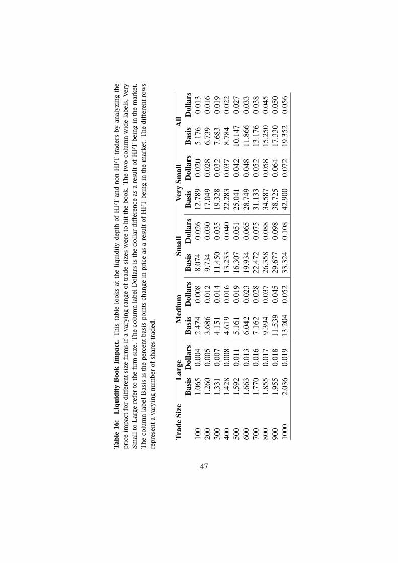
Tabl

e16

:L

iqui

dity

Boo

kIm

pact

.T

his

tabl

elo

oks

atth

eliq

uidi

tyde

pth

ofH

FTan

dno

n-H

FTtr

ader

sby

anal

yzin

gth

epr

ice

impa

ctfo

rdiff

eren

tsiz

efir

ms

ifa

vary

ing

rang

eof

trad

e-si

zes

wer

eto

hitt

hebo

ok.

The

two-

colu

mn

wid

ela

bels

,Ver

ySm

allt

oL

arge

refe

rto

the

firm

size

.The

colu

mn

labe

lDol

lars

isth

edo

llard

iffer

ence

asa

resu

ltof

HFT

bein

gin

the

mar

ket.

The

colu

mn

labe

lBas

isis

the

perc

entb

asis

poin

tsch

ange

inpr

ice

asa

resu

ltof

HFT

bein

gin

the

mar

ket.

The

diff

eren

trow

sre

pres

enta

vary

ing

num

bero

fsha

res

trad

ed.

Trad

eSi

zeL

arge

Med

ium

Smal

lVe

rySm

all

All

Bas

isD

olla

rsB

asis

Dol

lars

Bas

isD

olla

rsB

asis

Dol

lars

Bas

isD

olla

rs10

01.

065

0.00

42.

474

0.00

88.

074

0.02

612

.789

0.02

05.

176

0.01

320

01.

260

0.00

53.

686

0.01

29.

734

0.03

017

.049

0.02

86.

739

0.01

630

01.

331

0.00

74.

151

0.01

411

.450

0.03

519

.328

0.03

27.

683

0.01

940

01.

428

0.00

84.

619

0.01

613

.233

0.04

022

.283

0.03

78.

784

0.02

250

01.

592

0.01

15.

161

0.01

916

.307

0.05

125

.041

0.04

210

.147

0.02

760

01.

663

0.01

36.

042

0.02

319

.934

0.06

528

.749

0.04

811

.866

0.03

370

01.

770

0.01

67.

162

0.02

822

.472

0.07

531

.133

0.05

213

.176

0.03

880

01.

855

0.01

79.

394

0.03

726

.358

0.08

834

.587

0.05

815

.250

0.04

590

01.

955

0.01

811

.539

0.04

529

.677

0.09

838

.725

0.06

417

.330

0.05

010

002.

036

0.01

913

.204

0.05

233

.324

0.10

842

.900

0.07

219

.352

0.05

6

47

and decomposes the variance of the common component of the price to attributecontribution to the efficient price path between the two types of traders. The HFTprovide substantially more information to the price process than do non-HFT. TheHasbrouck methodologies utilized in this paper are similar to those found in Hen-dershott and Riordan (2009) and other papers.

6.2.1 Permanent Price Impact

To measure the information content of HFT and non-HFT trades I calculate thepermanent price impact of HFT and non-HFT trades. Hendershott and Riordan(2009) performed a similar calculation for trader types looking at algorithmictrading, while Barclay, Hendershott, and McCormick (2003) used the technique tocompare information from different markets. The HFT dataset is especially wellsuited for this as it is in milliseconds and thus avoids problems of multiple tradesoccurring in one time period, as occurs with data denoted in seconds. I estimatethe model on a trade-by-trade basis using 10 lags for HFT and non-HFT trades. Iestimate the model for each stock for each day. As in Barclay, Hendershott, andMcCormick (2003) and Hendershott and Riordan (2009), I estimate three equa-tions, a midpoint quote return equation, an HFT equation, and a non-HFT tradeequation. The time index, t, is based on event time, not clock time, and so eacht is an event that is a trade or quote change. qH is defined as the signed (+1 fora buy, -1 for a sell) HFT trades and qN is the similarly denoted signed non-HFTtrades. rt is defined as the quote midpoint to quote midpoint return between tradechanges. The 10-lag vector auto regression (VAR) is:

rt =10∑i=1

αirt−i +10∑i=0

βiqHt−i +

10∑i=0

γiqNt−i + ϵ1,t,

qHt =10∑i=1

δirt−i +10∑i=0

ρiqHt−i +

10∑i=0

ζiqNt−i + ϵ2,t,

qNt =10∑i=1

πirt−i +10∑i=0

νiqHt−i +

10∑i=0

ψiqNt−i + ϵ3,t.

After estimating the VAR model, I invert the VAR to get the vector movingaverage (VMA) model to obtain:

48

rtqHtqNt

=

a(L) b(L) c(L)d(L) e(L) f(L)g(L) h(L) i(L)

ϵ1,tϵ2,tϵ3,t

, (4)

where the vectors a(L) - i(L) are lag operators. Hasbrouck (1991a) interpretsthe impulse response function for HFT,

∑10t=0 b(L), as the private information con-

tent of an innovation in HFT trades. The non-HFT impulse response function is∑10t=0 c(L) and is the private information content of an innovation in non-HFT

trades. The impulse response function is a technology first used in the macro-economic literature to determine the impact of an exogenous shock to the econ-omy as it worked its way through the economy. Hasbrouck (1991a) and Has-brouck (1991b) took this methodology and applied it to the microstructure litera-ture. The expected portion of a trade should not impact prices and so should notshow up in the impulse response function; however, the unexpected portion, theinnovation, of a trade should influence the price of future trades. The impulseresponse function estimates this impact on future trades.

Table 17 shows the results of the HFT and non-HFT impulse response func-tion for 10 events into the future. There are 105 firms presented as fifteen stocksdo not contain enough data to calculate the VAR. Each stock is reported individ-ually. For each stock I estimate the statistical significance of the difference ofthe impulse response function for the HFT and Non-HFT 5 trading days usinga t-test. The t-test is adjusted using Newey-West standard errors to account forthe time-series correlation in observations. Also, I calculate the overall averageHFT and non-HFT impulse response function, this calculation incorporates theNewey-West correction for time series and also a correction for the cross-sectioncorrelation standard errors.

Of the 105 companies represented 90 of them have the HFT impulse responsefunction being larger than the non-HFT impulse response. None of the 15 firmswhere the non-HFT impulse response function is larger than HFT’s are statisti-cally significant. Of the 90 in the other direction, 26 of the differences are statisti-cally significant. On average, HFT’s impulse response function is 1.017 and NonHFT’s impulse response is 0.759. The overall difference is statistically signifi-cant. This suggests that HFT provide more private information than do non-HFTtrades. This is similar to the findings in Hendershott and Riordan (2009) withalgorithmic trades. Thus, an innovation in HFT trading tends to lead to a 34%greater permanent price change than does a trade by a non HFT.

49

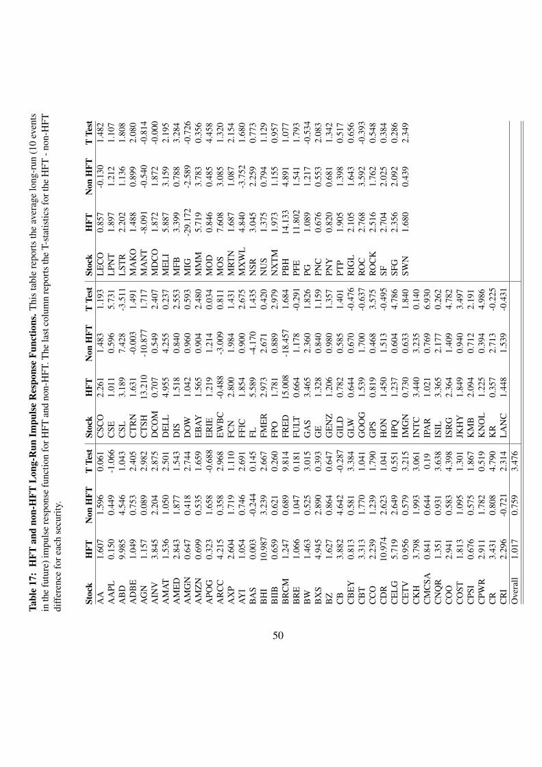
Tabl

e17

:H

FTan

dno

n-H

FTL

ong-

Run

Impu

lse

Res

pons

eFu

nctio

ns.T

his

tabl

ere

port

sth

eav

erag

elo

ng-r

un(1

0ev

ents

inth

efu

ture

)im

puls

ere

spon

sefu

nctio

nfo

rHFT

and

non-

HFT

.The

last

colu

mn

repo

rts

the

T-st

atis

tics

fort

heH

FT-n

on-H

FTdi

ffer

ence

fore

ach

secu

rity

.

Stoc

kH

FTN

onH

FTT

Test

Stoc

kH

FTN

onH

FTT

Test

Stoc

kH

FTN

onH

FTT

Test

AA

1.60

71.

596

0.06

1C

SCO

2.26

11.

483

1.19

3L

EC

O0.

857

-0.1

301.

482

AA

PL0.

150

0.44

9-1

.066

CSE

1.01

10.

596

5.73

1L

PNT

1.89

71.

212

1.10

7A

BD

9.98

54.

546

1.04

3C

SL3.

189

7.42

8-3

.511

LST

R2.

202

1.13

61.

808

AD

BE

1.04

90.

753

2.40

5C

TR

N1.

631

-0.0

031.

491

MA

KO

1.48

80.

899

2.08

0A

GN

1.15

70.

089

2.98

2C

TSH

13.2

10-1

0.87

71.

717

MA

NT

-8.0

91-0

.540

-0.8

14A

INV

3.84

52.

204

2.87

5D

CO

M0.

707

0.54

92.

407

MD

CO

1.87

21.

872

-0.0

00A

MA

T1.

536

1.05

02.

501

DE

LL

4.95

54.

255

0.23

7M

EL

I5.

887

3.15

92.

195

AM

ED

2.84

31.

877

1.54

3D

IS1.

518

0.84

02.

553

MFB

3.39

90.

788

3.28

4A

MG

N0.

647

0.41

82.

744

DO

W1.

042

0.96

00.

593

MIG

-29.

172

-2.5

89-0

.726

AM

ZN

0.69

90.

535

1.65

9E

BA

Y1.

565

0.90

42.

480

MM

M5.

719

3.78

30.

356

APO

G0.

323

1.65

8-0

.688

ER

IE1.

219

1.21

40.

034

MO

D0.

846

0.48

54.

458

AR

CC

4.21

50.

358

2.96

8E

WB

C-0

.488

-3.0

090.

811

MO

S7.

608

3.08

51.

320

AX

P2.

604

1.71

91.

110

FCN

2.80

01.

984

1.43

1M

RT

N1.

687

1.08

72.

154

AY

I1.

054

0.74

62.

691

FFIC

1.85

40.

900

2.67

5M

XW

L4.

840

-3.7

521.

680

BA

S0.

003

-0.2

440.

145

FL5.

589

-4.1

701.

435

NSR

3.04

52.

259

0.77

3B

HI

10.9

873.

239

2.66

7FM

ER

2.97

32.

671

0.42

0N

US

1.37

50.

794

1.12

9B

IIB

0.65

90.

621

0.26

0FP

O1.

781

0.88

92.

979

NX

TM

1.97

31.

155

0.95

7B

RC

M1.

247

0.68

99.

814

FRE

D15

.008

-18.

457

1.68

4PB

H14

.133

4.89

11.

077

BR

E1.

066

1.04

70.

181

FULT

0.66

41.

178

-0.2

91PF

E11

.802

1.54

11.

793

BW

1.46

30.

525

3.01

5G

AS

3.46

52.

360

1.82

6PG

1.08

91.

217

-0.5

34B

XS

4.94

52.

890

0.39

3G

E1.

328

0.84

01.

159

PNC

0.67

60.

553

2.08

3B

Z1.

627

0.86

40.

647

GE

NZ

1.20

60.

980

1.35

7PN

Y0.

820

0.68

11.

342

CB

3.88

24.

642

-0.2

87G

ILD

0.78

20.

585

1.40

1PT

P1.

905

1.39

80.

517

CB

EY

0.81

30.

581

3.38

4G

LW0.

644

0.67

0-0

.476

RIG

L2.

105

1.64

30.

656

CB

T3.

313

1.77

01.

041

GO

OG

1.53

91.

700

-0.6

37R

OC

2.76

83.

592

-0.3

93C

CO

2.23

91.

239

1.79

0G

PS0.

819

0.46

83.

575

RO

CK

2.51

61.

762

0.54

8C

DR

10.9

742.

623

1.04

1H

ON

1.45

01.

513

-0.4

95SF

2.70

42.

025

0.38

4C

EL

G5.

719

2.64

90.

551

HPQ

1.23

70.

604

4.78

6SF

G2.

356

2.09

20.

286

CE

TV

0.95

60.

579

3.21

5IM

GN

0.73

00.

633

1.84

0SW

N1.

680

0.43

92.

349

CK

H3.

798

1.99

33.

061

INT

C3.

440

3.23

50.

140

CM

CSA

0.84

10.

644

0.19

IPA

R1.

021

0.76

96.

930

CN

QR

1.35

10.

931

3.63

8IS

IL3.

365

2.17

70.

262

CO

O2.

941

0.58

34.

398

ISR

G2.

364

1.40

94.

782

CO

ST1.

813

1.09

51.

301

JKH

Y1.

849

0.94

03.

497

CPS

I0.

676

0.57

51.

867

KM

B2.

094

0.71

22.

191

CPW

R2.

911

1.78

20.

519

KN

OL

1.22

50.

394

4.98

6C

R3.

431

0.80

84.

790

KR

0.35

72.

713

-0.2

25C

RI

2.29

6-0

.721

2.31

4L

AN

C1.

448

1.53

9-0

.431

Ove

rall

1.01

70.

759

3.47

6

50

6.2.1.1 LR - SR Price Impact The results in table 17 show that HFT has alarger price impact than does non-HFT over the 10 period intervals. An item ofinterest is whether the price impact is immediate or gradual over the ten futuretime periods. Similar to the methodology used in Chaboud, Hjalmarsson, Vega,and Chiquoine (2009) and Hendershott and Riordan (2009), I test whether theprice process may cause an immediate overreaction to one type of trade and thatover the next nine periods in the future the impact decreases. If it is the casethat there is an immediate overreaction to a HFT trade this would support thetheory that HFT increase the volatility of markets. To analyze this I report thedifference between the long-run (LR; 10 event forecast horizon) and short-run(SR; immediate) impulse response functions in table 18.

Of the 105 The LR-SR impulse response is less for HFT than for non-HFTin 25 of the 105 firms. Of those 25 firms none are statistically significant. Ofthe 80 firms where the LR-SR impulse response function is greater for HFT thannon-HFT 15 are statistically significant. Also, for each market participant col-umn, a positive number implies that the LR impact of a trade is greater than theSR impact, and a negative number implies there is a short run overreaction andthat over the next nine periods the permanent price impact falls. The results oftable 18 suggest that HFT individual innovations have more private informationthan non-HFT trades and that the difference is persistent and increases beyond theimmediate impact of the trade.

6.2.2 Aggregate Amount of Information in HFT - Variance Decomposition

The permanent price impact section above shows that HFT demanded trades addimportant information to the market, but the methodology does not directly esti-mate the importance of HFT and non-HFT trading in the overall price formationprocess. To examine this I follow Hasbrouck (1991b) to decompose the varianceof the efficient price into the portion of total price discovery that is correlated withHFT and non-HFT trades. The results indicate which trades contribute more toprice discovery. The methodology decomposes the variance of the efficient priceinto the portion of total price discovery that is correlated with HFT and non-HFTtrades.

This analysis was also in Hendershott and Riordan (2009) to determine whetheralgorithmic or human traders contribute more to price discovery and I followa similar methodlogy. To perform the variance decomposition the return seriesrt(using midpoint returns to avoid the bid-ask bounce) into its random walk com-ponent mt and stationary component st: rt = mt + st.

mt represents the efficient price where mt = mt−1 + wt and wt is a random

51

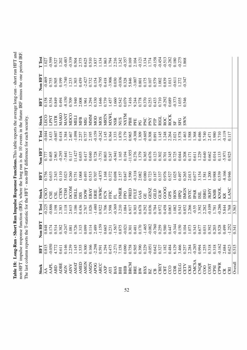
Tabl

e18

:L

ong-

Run

-Sho

rtR

unIm

puls

eR

espo

nse

Func

tions

.Thi

sta

ble

repo

rts

the

aver

age

long

-run

-sho

rtru

nH

FTan

dno

n-H

FTim

puls

ere

spon

sefu

nctio

n(I

RF)

,whe

reth

elo

ngru

nis

the

10ev

ents

inth

efu

ture

IRF

min

usth

eon

epe

riod

IRF.

The

last

colu

mn

repo

rts

the

T-st

atis

ticfo

rthe

HFT

-non

-HFT

diff

eren

cefo

reac

hse

curi

ty.

Stoc

kH

FTN

onH

FTT

Test

Stoc

kH

FTN

onH

FTT

Test

Stoc

kH

FTN

onH

FTT

Test

AA

0.81

50.

848

-0.2

25C

SCO

0.75

60.

777

-0.0

44L

EC

O0.

158

-0.4

691.

027

AA

PL-0

.050

0.17

4-0

.886

CSE

0.63

30.

405

3.43

3L

PNT

0.35

40.

755

-0.5

99A

BD

4.77

20.

514

1.19

8C

SL2.

343

2.96

3-0

.607

LST

R0.

849

0.50

50.

527

AD

BE

0.61

10.

382

2.38

3C

TR

N0.

110

-0.2

950.

418

MA

KO

0.49

40.

199

1.20

2A

GN

0.14

6-0

.247

1.11

8C

TSH

5.02

3-7

.641

1.38

4M

AN

T-8

.150

-3.7

40-0

.483

AIN

V2.

239

1.08

12.

615

DC

OM

0.26

00.

117

2.46

7M

DC

O0.

709

1.23

3-0

.339

AM

AT

1.14

50.

726

3.18

6D

EL

L0.

751

11.4

27-1

.098

ME

LI

1.94

01.

303

0.50

4A

ME

D1.

535

1.31

50.

436

DIS

1.06

80.

655

2.25

7M

FB2.

008

0.45

92.

375

AM

GN

0.30

00.

099

2.76

7D

OW

0.49

30.

417

0.75

7M

IG1.

961

-2.4

270.

625

AM

ZN

0.16

60.

114

1.02

6E

BA

Y0.

515

0.04

02.

195

MM

M3.

294

0.73

20.

510

APO

G-2

.298

2.48

9-1

.480

ER

IE0.

707

0.72

8-0

.159

MO

D0.

330

0.15

43.

837

AR

CC

0.59

1-1

.159

0.92

2E

WB

C-4

.875

-3.7

51-0

.242

MO

S1.

646

-0.7

951.

134

AX

P1.

294

0.66

51.

706

FCN

1.16

80.

803

1.14

5M

RT

N0.

739

0.41

81.

863

AY

I0.

475

0.23

13.

598

FFIC

0.37

20.

247

0.36

4M

XW

L1.

457

-3.9

061.

794

BA

S-2

.271

-1.5

67-0

.369

FL0.

698

-6.9

411.

333

NSR

1.66

00.

030

2.21

6B

HI

7.15

80.

875

3.21

0FM

ER

2.15

71.

165

1.87

0N

US

0.54

2-0

.036

1.24

2B

IIB

0.09

0-0

.021

1.08

4FP

O0.

847

0.19

43.

179

NX

TM

0.07

90.

328

-0.3

57B

RC

M0.

758

0.30

16.

917

FRE

D3.

590

-11.

955

0.96

5PB

H7.

416

5.84

60.

169

BR

E0.

505

0.48

10.

303

FULT

-0.3

180.

276

-0.3

08PF

E9.

244

-3.0

072.

104

BW

0.39

00.

170

0.67

8G

AS

2.08

21.

379

1.30

9PG

0.77

80.

801

-0.1

21B

XS

0.22

9-1

.465

0.29

2G

E0.

080

0.36

5-0

.605

PNC

0.37

00.

175

3.13

4B

Z-0

.051

-0.0

820.

036

GE

NZ

0.72

30.

676

0.30

8PN

Y0.

253

0.10

71.

774

CB

0.64

2-0

.760

0.78

4G

ILD

0.18

70.

123

0.89

1PT

P0.

433

0.57

9-0

.158

CB

EY

0.32

70.

259

0.97

2G

LW0.

337

0.30

21.

145

RIG

L0.

710

1.00

2-0

.454

CB

T1.

182

0.58

00.

458

GO

OG

0.97

60.

701

1.24

8R

OC

-0.2

920.

839

-0.5

13C

CO

0.48

40.

447

0.06

3G

PS0.

527

0.34

52.

264

RO

CK

0.68

91.

013

-0.2

82C

DR

6.12

9-0

.344

1.08

2H

ON

1.02

50.

725

2.02

1SF

-0.3

73-0

.611

0.18

0C

EL

G3.

466

0.15

00.

543

HPQ

0.49

70.

044

3.57

8SF

G1.

035

1.27

2-0

.275

CE

TV

0.25

70.

104

0.85

2IM

GN

0.26

50.

208

1.46

3SW

N0.

546

-0.3

471.

868

CK

H2.

284

1.07

32.

266

INT

C2.

013

0.17

11.

588

CM

CSA

-0.2

850.

343

-0.5

5IP

AR

0.67

70.

611

1.36

8C

NQ

R0.

994

0.67

73.

392

ISIL

3.15

41.

229

0.48

6C

OO

1.25

50.

031

2.28

2IS

RG

1.58

10.

640

5.74

0C

OST

0.31

80.

392

-0.1

09JK

HY

1.20

00.

662

2.47

1C

PSI

0.31

80.

203

1.78

1K

MB

0.98

80.

014

1.98

0C

PWR

-0.1

620.

528

-0.2

86K

NO

L0.

539

0.13

33.

710

CR

2.68

40.

499

5.84

4K

R-8

.166

-5.9

71-0

.119

CR

I0.

623

-1.2

521.

768

LA

NC

0.94

60.

925

0.11

7O

vera

ll0.

515

0.34

13.

563

52

walk with Ewt = 0; st is the non-persistent price component. Let σ2ϵ1

= Eϵ21, σ2ϵ2

= Eϵ22, and σ2ϵ3

= Eϵ23, I decompose the variance of the efficient price mt intotrade-correlated and trade-uncorrelated changes:

σ2w = (

10∑i=0

ai)2σ2

ϵ1+ (

10∑i=0

bi)2σ2

ϵ2+ (

10∑i=0

ci)2σ2

ϵ3, (5)

where the a, b, c are as defined in the previous section as the lag coefficientsfound in the VMA matrix. The (

∑10i=0 bi)

2σ2ϵ2

term represents the proportion of theefficient price variance attributable to HFT and the (

∑10i=0 ci)

2σ2ϵ3

term representsthe non-HFT proportion of the efficient price variance. The (

∑10i=0 ai)

2σ2ϵ1

term isthe already public information portion of price discovery.

The results from this exercise are found in table 19. I report the average con-tribution by HFT and by non HFT for each company over the five days. The finalcolumn is the t-statistic for the difference between the HFT and non-HFT contri-bution and is adjusted for its time-series correlation with Newey-West standarderrors. I also report the average overall contribution, whose t-statistic is correctedfor time-series correlation and for cross-sectional correlation. The HFT is the con-tribution to price discovery from HFT, and the same interpretation is true with thenon-HFT column. The contribution to the Returns component (the public infor-mation) is the public information related to price discovery, it is unreported herefor lack of space, but can be easily calculated by taking the difference between 1and the sum of the HFT and non-HFT components.

Of the 118 firms 68 of them show HFT as having a greater contribution toprice discovery, and 28 of those stocks’ HFT - non-HFT contribution differenceis statistically significant. In the 50 stocks where the non-HFT contribution isgreater than that of the HFT, the difference is statistically significant for 7 firms.On average HFT contributes 86% more to price discovery than do non-HFT.

6.2.3 Information Share

This section examines the role HFT and non-HFT quotes play in the price dis-covery process, whereas the previous two sections had been analyzing the roleof trades. I use the Information Shares (IS) approach introduced by Hasbrouck(1995) and that is used in, among others, Chaboud, Hjalmarsson, Vega, and Chiquoine(2009) and Hendershott and Riordan (2009). This approach has been used to de-termine which of several markets contributes more to price discovery, and, as willbe done here, to determine which type of market participant contributes more tothe price discovery process.

53

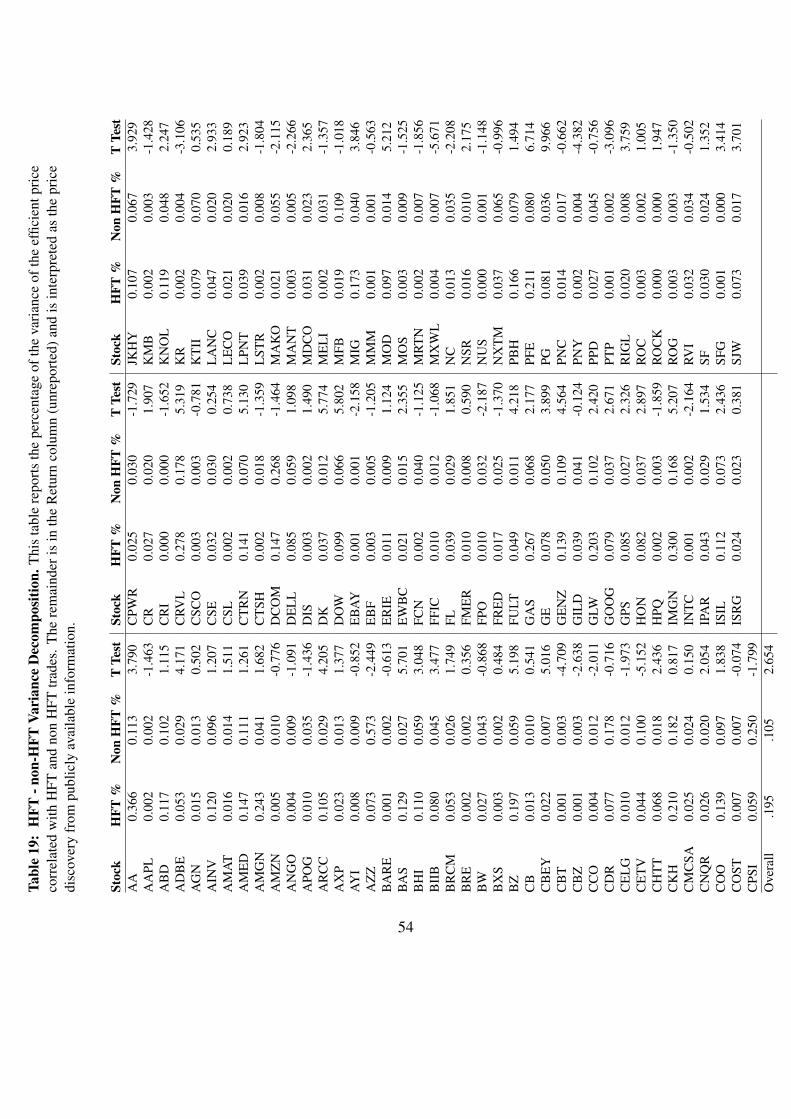
Tabl

e19

:H

FT-n

on-H

FTVa

rian

ceD

ecom

posi

tion.

Thi

sta

ble

repo

rts

the

perc

enta

geof

the

vari

ance

ofth

eef

ficie

ntpr

ice

corr

elat

edw

ithH

FTan

dno

nH

FTtr

ades

.T

here

mai

nder

isin

the

Ret

urn

colu

mn

(unr

epor

ted)

and

isin

terp

rete

das

the

pric

edi

scov

ery

from

publ

icly

avai

labl

ein

form

atio

n.

Stoc

kH

FT%

Non

HFT

%T

Test

Stoc

kH

FT%

Non

HFT

%T

Test

Stoc

kH

FT%

Non

HFT

%T

Test

AA

0.36

60.

113

3.79

0C

PWR

0.02

50.

030

-1.7

29JK

HY

0.10

70.

067

3.92

9A

APL

0.00

20.

002

-1.4

63C

R0.

027

0.02

01.

907

KM

B0.

002

0.00

3-1

.428

AB

D0.

117

0.10

21.

115

CR

I0.

000

0.00

0-1

.652

KN

OL

0.11

90.

048

2.24

7A

DB

E0.

053

0.02

94.

171

CRV

L0.

278

0.17

85.

319

KR

0.00

20.

004

-3.1

06A

GN

0.01

50.

013

0.50

2C

SCO

0.00

30.

003

-0.7

81K

TII

0.07

90.

070

0.53

5A

INV

0.12

00.

096

1.20

7C

SE0.

032

0.03

00.

254

LA

NC

0.04

70.

020

2.93

3A

MA

T0.

016

0.01

41.

511

CSL

0.00

20.

002

0.73

8L

EC

O0.

021

0.02

00.

189

AM

ED

0.14

70.

111

1.26

1C

TR

N0.

141

0.07

05.

130

LPN

T0.

039

0.01

62.

923

AM

GN

0.24

30.

041

1.68

2C

TSH

0.00

20.

018

-1.3

59L

STR

0.00

20.

008

-1.8

04A

MZ

N0.

005

0.01

0-0

.776

DC

OM

0.14

70.

268

-1.4

64M

AK

O0.

021

0.05

5-2

.115

AN

GO

0.00

40.

009

-1.0

91D

EL

L0.

085

0.05

91.

098

MA

NT

0.00

30.

005

-2.2

66A

POG

0.01

00.

035

-1.4

36D

IS0.

003

0.00

21.

490

MD

CO

0.03

10.

023

2.36

5A

RC

C0.

105

0.02

94.

205

DK

0.03

70.

012

5.77

4M

EL

I0.

002

0.03

1-1

.357

AX

P0.

023

0.01

31.

377

DO

W0.

099

0.06

65.

802

MFB

0.01

90.

109

-1.0

18A

YI

0.00

80.

009

-0.8

52E

BA

Y0.

001

0.00

1-2

.158

MIG

0.17

30.

040

3.84

6A

ZZ

0.07

30.

573

-2.4

49E

BF

0.00

30.

005

-1.2

05M

MM

0.00

10.

001

-0.5

63B

AR

E0.

001

0.00

2-0

.613

ER

IE0.

011

0.00

91.

124

MO

D0.

097

0.01

45.

212

BA

S0.

129

0.02

75.

701

EW

BC

0.02

10.

015

2.35

5M

OS

0.00

30.

009

-1.5

25B

HI

0.11

00.

059

3.04

8FC

N0.

002

0.04

0-1

.125

MR

TN

0.00

20.

007

-1.8

56B

IIB

0.08

00.

045

3.47

7FF

IC0.

010

0.01

2-1

.068

MX

WL

0.00

40.

007

-5.6

71B

RC

M0.

053

0.02

61.

749

FL0.

039

0.02

91.

851

NC

0.01

30.

035

-2.2

08B

RE

0.00

20.

002

0.35

6FM

ER

0.01

00.

008

0.59

0N

SR0.

016

0.01

02.

175

BW

0.02

70.

043

-0.8

68FP

O0.

010

0.03

2-2

.187

NU

S0.

000

0.00

1-1

.148

BX

S0.

003

0.00

20.

484

FRE

D0.

017

0.02

5-1

.370

NX

TM

0.03

70.

065

-0.9

96B

Z0.

197

0.05

95.

198

FULT

0.04

90.

011

4.21

8PB

H0.

166

0.07

91.

494

CB

0.01

30.

010

0.54

1G

AS

0.26

70.

068

2.17

7PF

E0.

211

0.08

06.

714

CB

EY

0.02

20.

007

5.01

6G

E0.

078

0.05

03.

899

PG0.

081

0.03

69.

966

CB

T0.

001

0.00

3-4

.709

GE

NZ

0.13

90.

109

4.56

4PN

C0.

014

0.01

7-0

.662

CB

Z0.

001

0.00

3-2

.638

GIL

D0.

039

0.04

1-0

.124

PNY

0.00

20.

004

-4.3

82C

CO

0.00

40.

012

-2.0

11G

LW0.

203

0.10

22.

420

PPD

0.02

70.

045

-0.7

56C

DR

0.07

70.

178

-0.7

16G

OO

G0.

079

0.03

72.

671

PTP

0.00

10.

002

-3.0

96C

EL

G0.

010

0.01

2-1

.973

GPS

0.08

50.

027

2.32

6R

IGL

0.02

00.

008

3.75

9C

ET

V0.

044

0.10

0-5

.152

HO

N0.

082

0.03

72.

897

RO

C0.

003

0.00

21.

005

CH

TT

0.06

80.

018

2.43

6H

PQ0.

002

0.00

3-1

.859

RO

CK

0.00

00.

000

1.94

7C

KH

0.21

00.

182

0.81

7IM

GN

0.30

00.

168

5.20

7R

OG

0.00

30.

003

-1.3

50C

MC

SA0.

025

0.02

40.

150

INT

C0.

001

0.00

2-2

.164

RVI

0.03

20.

034

-0.5

02C

NQ

R0.

026

0.02

02.

054

IPA

R0.

043

0.02

91.

534

SF0.

030

0.02

41.

352

CO

O0.

139

0.09

71.

838

ISIL

0.11

20.

073

2.43

6SF

G0.

001

0.00

03.

414

CO

ST0.

007

0.00

7-0

.074

ISR

G0.

024

0.02

30.

381

SJW

0.07

30.

017

3.70

1C

PSI

0.05

90.

250

-1.7

99O

vera

ll.1

95.1

052.

654

54

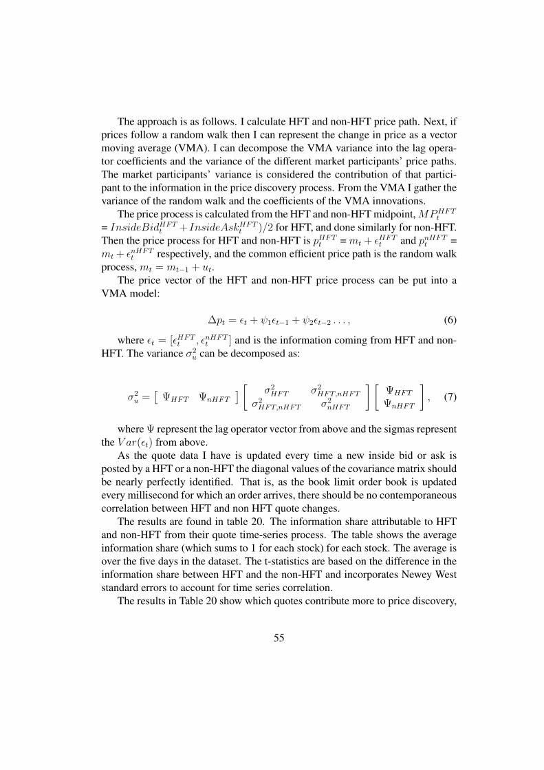
The approach is as follows. I calculate HFT and non-HFT price path. Next, ifprices follow a random walk then I can represent the change in price as a vectormoving average (VMA). I can decompose the VMA variance into the lag opera-tor coefficients and the variance of the different market participants’ price paths.The market participants’ variance is considered the contribution of that partici-pant to the information in the price discovery process. From the VMA I gather thevariance of the random walk and the coefficients of the VMA innovations.

The price process is calculated from the HFT and non-HFT midpoint,MPHFTt

= InsideBidHFTt +InsideAskHFT

t )/2 for HFT, and done similarly for non-HFT.Then the price process for HFT and non-HFT is pHFT

t = mt + ϵHFTt and pnHFT

t =mt + ϵnHFT

t respectively, and the common efficient price path is the random walkprocess, mt = mt−1 + ut.

The price vector of the HFT and non-HFT price process can be put into aVMA model:

∆pt = ϵt + ψ1ϵt−1 + ψ2ϵt−2 . . . , (6)

where ϵt = [ϵHFTt , ϵnHFT

t ] and is the information coming from HFT and non-HFT. The variance σ2

u can be decomposed as:

σ2u =

[ΨHFT ΨnHFT

] [ σ2HFT σ2

HFT,nHFT

σ2HFT,nHFT σ2

nHFT

] [ΨHFT

ΨnHFT

], (7)

where Ψ represent the lag operator vector from above and the sigmas representthe V ar(ϵt) from above.

As the quote data I have is updated every time a new inside bid or ask isposted by a HFT or a non-HFT the diagonal values of the covariance matrix shouldbe nearly perfectly identified. That is, as the book limit order book is updatedevery millisecond for which an order arrives, there should be no contemporaneouscorrelation between HFT and non HFT quote changes.

The results are found in table 20. The information share attributable to HFTand non-HFT from their quote time-series process. The table shows the averageinformation share (which sums to 1 for each stock) for each stock. The average isover the five days in the dataset. The t-statistics are based on the difference in theinformation share between HFT and the non-HFT and incorporates Newey Weststandard errors to account for time series correlation.

The results in Table 20 show which quotes contribute more to price discovery,

55

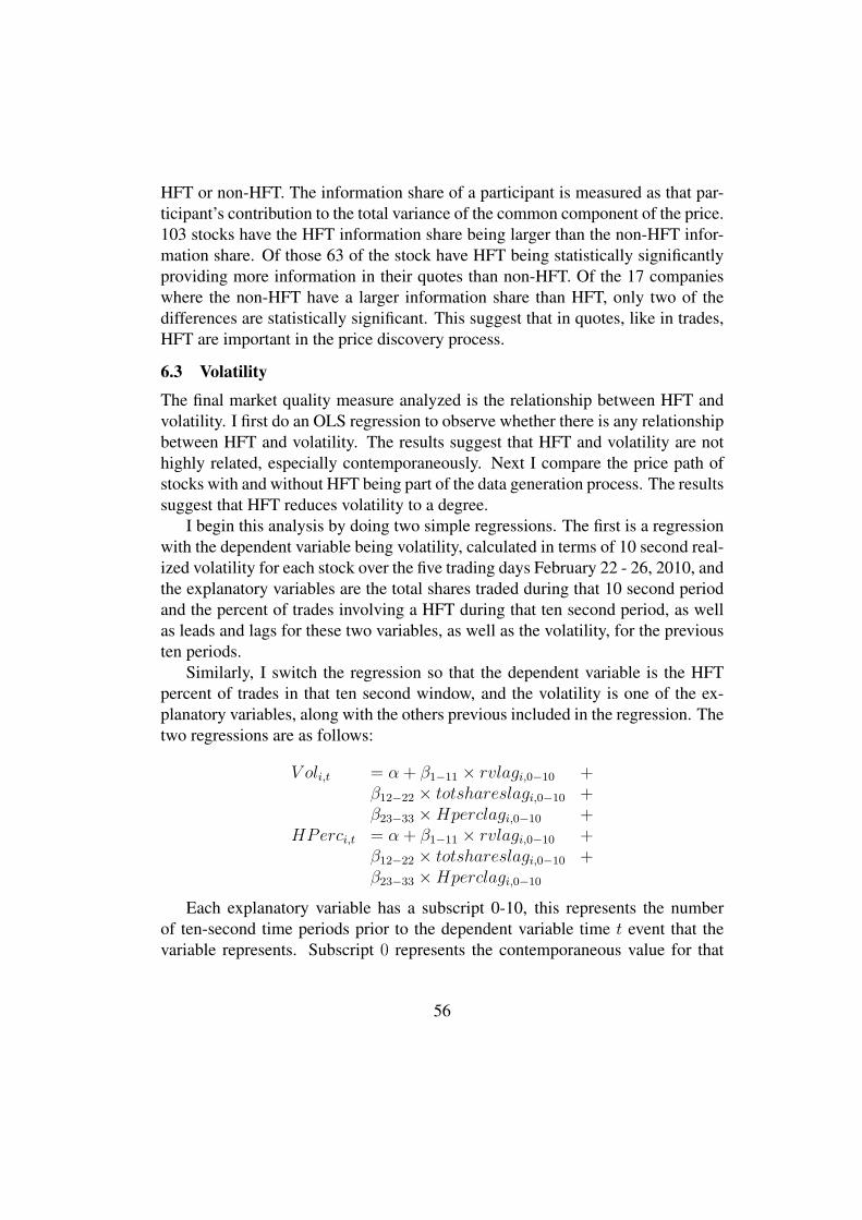
HFT or non-HFT. The information share of a participant is measured as that par-ticipant’s contribution to the total variance of the common component of the price.103 stocks have the HFT information share being larger than the non-HFT infor-mation share. Of those 63 of the stock have HFT being statistically significantlyproviding more information in their quotes than non-HFT. Of the 17 companieswhere the non-HFT have a larger information share than HFT, only two of thedifferences are statistically significant. This suggest that in quotes, like in trades,HFT are important in the price discovery process.

6.3 Volatility

The final market quality measure analyzed is the relationship between HFT andvolatility. I first do an OLS regression to observe whether there is any relationshipbetween HFT and volatility. The results suggest that HFT and volatility are nothighly related, especially contemporaneously. Next I compare the price path ofstocks with and without HFT being part of the data generation process. The resultssuggest that HFT reduces volatility to a degree.

I begin this analysis by doing two simple regressions. The first is a regressionwith the dependent variable being volatility, calculated in terms of 10 second real-ized volatility for each stock over the five trading days February 22 - 26, 2010, andthe explanatory variables are the total shares traded during that 10 second periodand the percent of trades involving a HFT during that ten second period, as wellas leads and lags for these two variables, as well as the volatility, for the previousten periods.

Similarly, I switch the regression so that the dependent variable is the HFTpercent of trades in that ten second window, and the volatility is one of the ex-planatory variables, along with the others previous included in the regression. Thetwo regressions are as follows:

V oli,t = α+ β1−11 × rvlagi,0−10 +β12−22 × totshareslagi,0−10 +β23−33 ×Hperclagi,0−10 +

HPerci,t = α+ β1−11 × rvlagi,0−10 +β12−22 × totshareslagi,0−10 +β23−33 ×Hperclagi,0−10

Each explanatory variable has a subscript 0-10, this represents the numberof ten-second time periods prior to the dependent variable time t event that thevariable represents. Subscript 0 represents the contemporaneous value for that

56

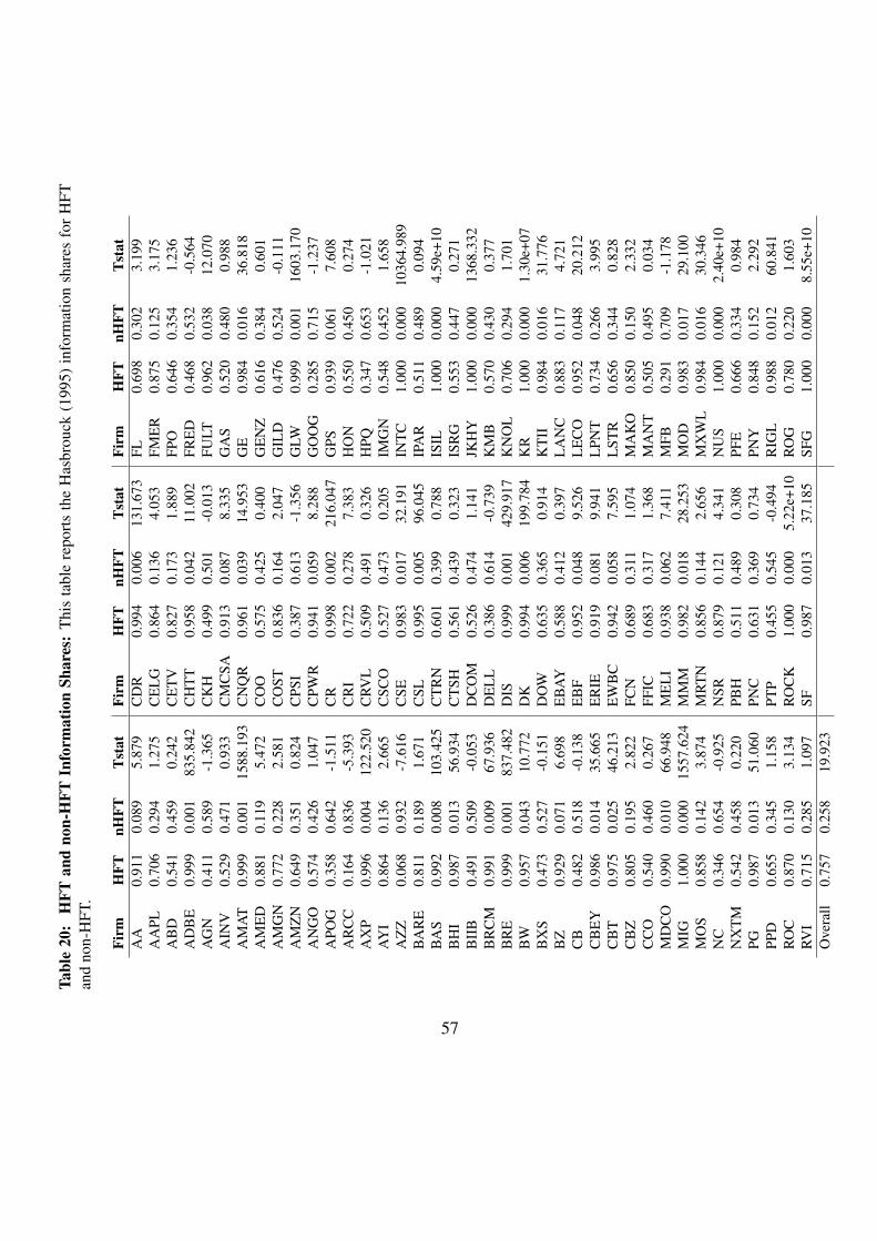
Tabl

e20

:H

FTan

dno

n-H

FTIn

form

atio

nSh

ares

:T

his

tabl

ere

port

sth

eH

asbr

ouck

(199

5)in

form

atio

nsh

ares

for

HFT

and

non-

HFT

.

Firm

HFT

nHFT

Tst

atFi

rmH

FTnH

FTT

stat

Firm

HFT

nHFT

Tst

atA

A0.

911

0.08

95.

879

CD

R0.

994

0.00

613

1.67

3FL

0.69

80.

302

3.19

9A

APL

0.70

60.

294

1.27

5C

EL

G0.

864

0.13

64.

053

FME

R0.

875

0.12

53.

175

AB

D0.

541

0.45

90.

242

CE

TV

0.82

70.

173

1.88

9FP

O0.

646

0.35

41.

236

AD

BE

0.99

90.

001

835.

842

CH

TT

0.95

80.

042

11.0

02FR

ED

0.46

80.

532

-0.5

64A

GN

0.41

10.

589

-1.3

65C

KH

0.49

90.

501

-0.0

13FU

LT0.

962

0.03

812

.070

AIN

V0.

529

0.47

10.

933

CM

CSA

0.91

30.

087

8.33

5G

AS

0.52

00.

480

0.98

8A

MA

T0.

999

0.00

115

88.1

93C

NQ

R0.

961

0.03

914

.953

GE

0.98

40.

016

36.8

18A

ME

D0.

881

0.11

95.

472

CO

O0.

575

0.42

50.

400

GE

NZ

0.61

60.

384

0.60

1A

MG

N0.

772

0.22

82.

581

CO

ST0.

836

0.16

42.

047

GIL

D0.

476

0.52

4-0

.111

AM

ZN

0.64

90.

351

0.82

4C

PSI

0.38

70.

613

-1.3

56G

LW0.

999

0.00

116

03.1

70A

NG

O0.

574

0.42

61.

047

CPW

R0.

941

0.05

98.

288

GO

OG

0.28

50.

715

-1.2

37A

POG

0.35

80.

642

-1.5

11C

R0.

998

0.00

221

6.04

7G

PS0.

939

0.06

17.

608

AR

CC

0.16

40.

836

-5.3

93C

RI

0.72

20.

278

7.38

3H

ON

0.55

00.

450

0.27

4A

XP

0.99

60.

004

122.

520

CRV

L0.

509

0.49

10.

326

HPQ

0.34

70.

653

-1.0

21A

YI

0.86

40.

136

2.66

5C

SCO

0.52

70.

473

0.20

5IM

GN

0.54

80.

452

1.65

8A

ZZ

0.06

80.

932

-7.6

16C

SE0.

983

0.01

732

.191

INT

C1.

000

0.00

010

364.

989

BA

RE

0.81

10.

189

1.67

1C

SL0.

995

0.00

596

.045

IPA

R0.

511

0.48

90.

094

BA

S0.

992

0.00

810

3.42

5C

TR

N0.

601

0.39

90.

788

ISIL

1.00

00.

000

4.59

e+10

BH

I0.

987

0.01

356

.934

CT

SH0.

561

0.43

90.

323

ISR

G0.

553

0.44

70.

271

BII

B0.

491

0.50

9-0

.053

DC

OM

0.52

60.

474

1.14

1JK

HY

1.00

00.

000

1368

.332

BR

CM

0.99

10.

009

67.9

36D

EL

L0.

386

0.61

4-0

.739

KM

B0.

570

0.43

00.

377

BR

E0.

999

0.00

183

7.48

2D

IS0.

999

0.00

142

9.91

7K

NO

L0.

706

0.29

41.

701

BW

0.95

70.

043

10.7

72D

K0.

994

0.00

619

9.78

4K

R1.

000

0.00

01.

30e+

07B

XS

0.47

30.

527

-0.1

51D

OW

0.63

50.

365

0.91

4K

TII

0.98

40.

016

31.7

76B

Z0.

929

0.07

16.

698

EB

AY

0.58

80.

412

0.39

7L

AN

C0.

883

0.11

74.

721

CB

0.48

20.

518

-0.1

38E

BF

0.95

20.

048

9.52

6L

EC

O0.

952

0.04

820

.212

CB

EY

0.98

60.

014

35.6

65E

RIE

0.91

90.

081

9.94

1L

PNT

0.73

40.

266

3.99

5C

BT

0.97

50.

025

46.2

13E

WB

C0.

942

0.05

87.

595

LST

R0.

656

0.34

40.

828

CB

Z0.

805

0.19

52.

822

FCN

0.68

90.

311

1.07

4M

AK

O0.

850

0.15

02.

332

CC

O0.

540

0.46

00.

267

FFIC

0.68

30.

317

1.36

8M

AN

T0.

505

0.49

50.

034

MD

CO

0.99

00.

010

66.9

48M

EL

I0.

938

0.06

27.

411

MFB

0.29

10.

709

-1.1

78M

IG1.

000

0.00

015

57.6

24M

MM

0.98

20.

018

28.2

53M

OD

0.98

30.

017

29.1

00M

OS

0.85

80.

142

3.87

4M

RT

N0.

856

0.14

42.

656

MX

WL

0.98

40.

016

30.3

46N

C0.

346

0.65

4-0

.925

NSR

0.87

90.

121

4.34

1N

US

1.00

00.

000

2.40

e+10

NX

TM

0.54

20.

458

0.22

0PB

H0.

511

0.48

90.

308

PFE

0.66

60.

334

0.98

4PG

0.98

70.

013

51.0

60PN

C0.

631

0.36

90.

734

PNY

0.84

80.

152

2.29

2PP

D0.

655

0.34

51.

158

PTP

0.45

50.

545

-0.4

94R

IGL

0.98

80.

012

60.8

41R

OC

0.87

00.

130

3.13

4R

OC

K1.

000

0.00

05.

22e+

10R

OG

0.78

00.

220

1.60

3RV

I0.

715

0.28

51.

097

SF0.

987

0.01

337

.185

SFG

1.00

00.

000

8.55

e+10

Ove

rall

0.75

70.

258

19.9

23

57

variable. Volatility is defined as, for example using the fourth lag, rvlag4 =(log(pricei,t−5/pricei,t4))

2. The betas represent row vectors of 1x11 and the ex-planatory variables column vectors of 11x1. rv is the squared price change forcompany i for the respective time period. totshares is the number of shares thatwere traded for a company i in that ten second time period. Hperc is the percentof trades for stock i in that time period for which HFT were involved.

Table 21 shows the results of the two regressions and only reports the variablesof interest HFT trading percent “HFT%” for the first regression and “RV ” forthe second regresion. In the first two columns are the results of the first regressionwith volatility as the dependent variable. The last two columns display the resultfor the second regression with HFT percent of trading as the dependent variable.For both, only the results of the variables of interest are shown. The results suggestthat there is some statistically significant relationship between the two variables.when Volatility is the dependent variable, the Percent of HFT trading coefficientis statistically significant and negative in the two period lag period.

In the second regression, with HFT Percent as the dependent variable, manyof the prior volatility coefficients are statistically significant. The periods lag 1, 2,5, 9, and 10 statistically significant. All of the statistically significant lag coeffi-cients are positive except for period 9. This suggests that after volatility has beenelevated HFT tend to make up more of the market trades. Of course, because ofthe endogeneity problem and econometric issues not much weight should be puton these results. I include them only to show that there might be a relationshipbetween HFT and volatility. The next section attempts to avoid the econometricissues and to reduce the endogeneity problem.

6.3.0.1 HFT Impact on Volatility I next try to disentangle the HFT - Volatil-ity relationship and minimize the endogeneity problem. To reduce the impact ofendogeneity, I take advantage of the book data I have available in one minute in-crements. With this data I can estimate what the price impact would have beenhad there been no HFT demanding liquidity or supplying liquidity. That is, I havethe actual price series for each stock, but I can supplement that with the hypo-thetical price series of each stock assuming that there were no HFT in the market.Table 22, 23, and 24 shows the results. For each stock I calculate the realizedvolatility, the sum over one minute increments of the absolute value of the returnsover the day. I perform this calculation for each stock on each day and do it forthe actual price path, and also for an alternative price path based on the role ofHFT. In table 22 I remove HFT initiated trades and also HFT liquidity providingtrades. Thus, were the realized volatility calculation would have used a trade by

58

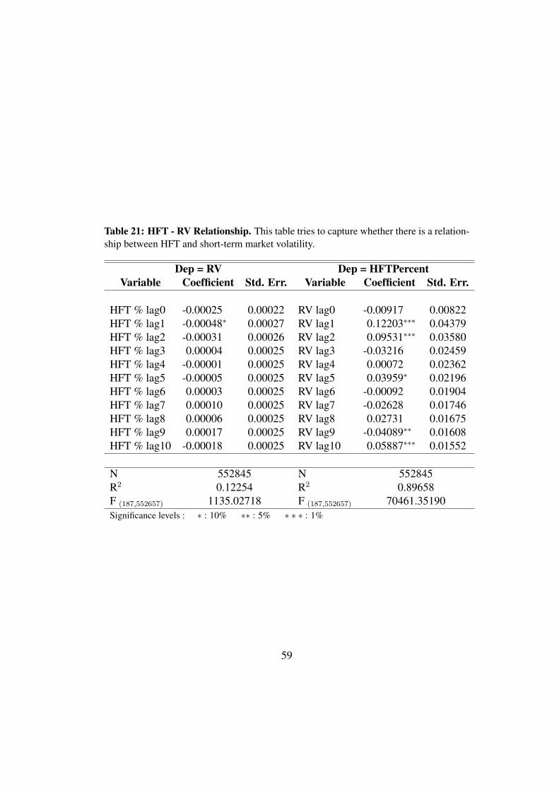
Table 21: HFT - RV Relationship. This table tries to capture whether there is a relation-ship between HFT and short-term market volatility.

Dep = RV Dep = HFTPercentVariable Coefficient Std. Err. Variable Coefficient Std. Err.

HFT % lag0 -0.00025 0.00022 RV lag0 -0.00917 0.00822HFT % lag1 -0.00048∗ 0.00027 RV lag1 0.12203∗∗∗ 0.04379HFT % lag2 -0.00031 0.00026 RV lag2 0.09531∗∗∗ 0.03580HFT % lag3 0.00004 0.00025 RV lag3 -0.03216 0.02459HFT % lag4 -0.00001 0.00025 RV lag4 0.00072 0.02362HFT % lag5 -0.00005 0.00025 RV lag5 0.03959∗ 0.02196HFT % lag6 0.00003 0.00025 RV lag6 -0.00092 0.01904HFT % lag7 0.00010 0.00025 RV lag7 -0.02628 0.01746HFT % lag8 0.00006 0.00025 RV lag8 0.02731 0.01675HFT % lag9 0.00017 0.00025 RV lag9 -0.04089∗∗ 0.01608HFT % lag10 -0.00018 0.00025 RV lag10 0.05887∗∗∗ 0.01552

N 552845 N 552845R2 0.12254 R2 0.89658F (187,552657) 1135.02718 F (187,552657) 70461.35190Significance levels : ∗ : 10% ∗∗ : 5% ∗ ∗ ∗ : 1%

59

a HFT initiated trade, it instead has to grab the price from the next trade that isinitiated by a non-HFT. Also, when the realized volatility would have had a tradewhere a HFT was providing the liquidity, I adjust the price based on the size of thetrade and the price impact it would have on the book after removing the HFT bookentries. Table 23 does the same calculation but only removes the HFT liquidityproviding trades. Finally, table 24 removes only the HFT initiated trades from thealternative price path.

In table 22 of the 120 stocks, only one exhibits that volatility would not bereduced if HFT had not been in the market. Of those where HFT reduced thevolatility, 85 of them have volatility that is statistically significantly less thanwhat it would be if HFT had not been part of the market. The t statistics forthe individual firms use Newey-West standard errors to account for the time se-ries correlation. the overall t-statistic also corrects for cross-sectional correlation.These results suggest that HFT help to reduce the volatility in the market.

Table 23 looks at what happens when HFT is only removed from providingliquidity. Only one firm shows that volatility is increased by removing HFT fromproviding liquidity. Of the 119 that show HFT is reduced, 82 show a statisti-cally significant difference in volatility. The t statistics for the individual firms useNewey-West standard errors to account for the time series correlation. the overallt-statistic also corrects for cross-sectional correlation. This is the mechanical por-tion of the HFT price reduction: when liquidity is removed, the only way pricescan move is further away from their previous path, thus increasing volatility.

Table 24 again compares the realized volatility of the 120 firms, but it com-pares the volatility of the actual price path with the volatility of the price path ifonly HFT initiated trades are removed. Table 24, unlike the previous table, mayshow a positive, negative, or no direction in its impact on volatility. Of the 120firms, 72 of them have a higher volatility when HFT initiated trades are present.Thus, a small majority of firms experience slightly higher volatility with HFTinitiated trades. However of these 72 stocks, only one is statistically significant.Of the 48 stocks where the presence of HFT initiated trades reduces volatilitynone show a statistically significant difference in volatility. The t statistics forthe individual firms use Newey-West standard errors to account for the time se-ries correlation. the overall t-statistic also corrects for cross-sectional correlation.These results suggest that HFT initiated trades do not result in increased volatility.

60

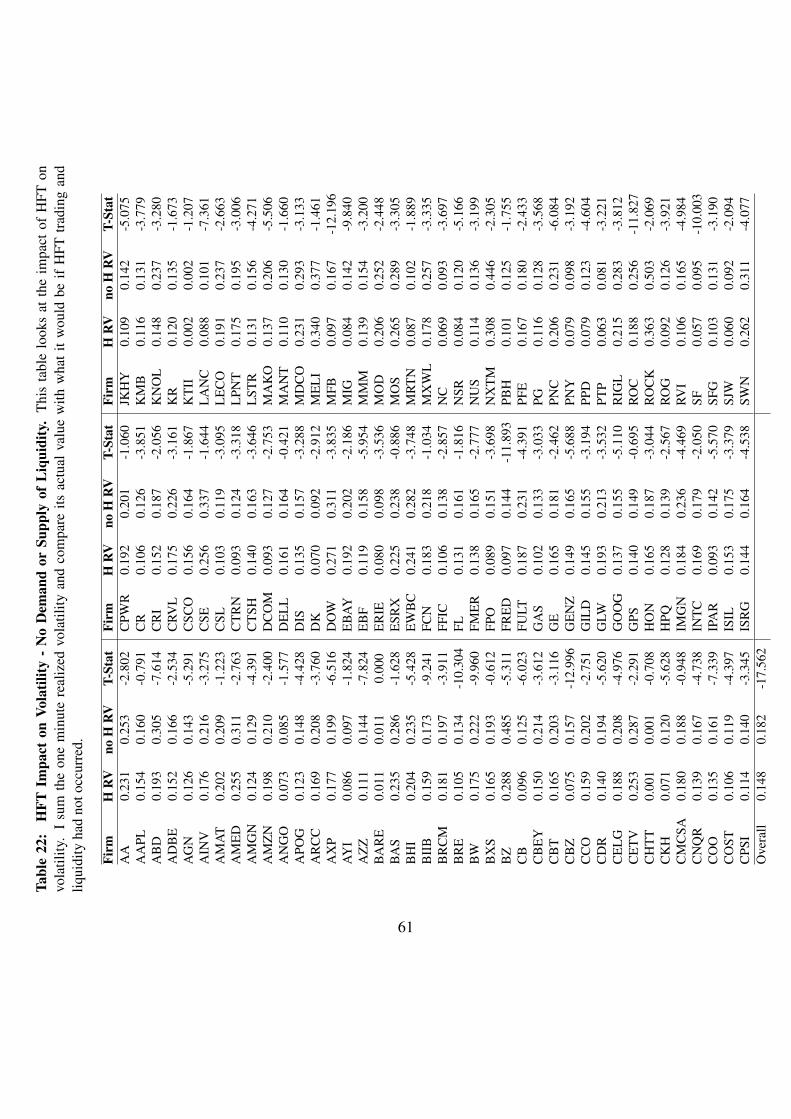
Tabl

e22

:H

FTIm

pact

onVo

latil

ity-

No

Dem

and

orSu

pply

ofL

iqui

dity

.T

his

tabl

elo

oks

atth

eim

pact

ofH

FTon

vola

tility

.I

sum

the

one

min

ute

real

ized

vola

tility

and

com

pare

itsac

tual

valu

ew

ithw

hat

itw

ould

beif

HFT

trad

ing

and

liqui

dity

had

noto

ccur

red.

Firm

HR

Vno

HR

VT-

Stat

Firm

HR

Vno

HR

VT-

Stat

Firm

HR

Vno

HR

VT-

Stat

AA

0.23

10.

253

-2.8

02C

PWR

0.19

20.

201

-1.0

60JK

HY

0.10

90.

142

-5.0

75A

APL

0.15

40.

160

-0.7

91C

R0.

106

0.12

6-3

.851

KM

B0.

116

0.13

1-3

.779

AB

D0.

193

0.30

5-7

.614

CR

I0.

152

0.18

7-2

.056

KN

OL

0.14

80.

237

-3.2

80A

DB

E0.

152

0.16

6-2

.534

CRV

L0.

175

0.22

6-3

.161

KR

0.12

00.

135

-1.6

73A

GN

0.12

60.

143

-5.2

91C

SCO

0.15

60.

164

-1.8

67K

TII

0.00

20.

002

-1.2

07A

INV

0.17

60.

216

-3.2

75C

SE0.

256

0.33

7-1

.644

LA

NC

0.08

80.

101

-7.3

61A

MA

T0.

202

0.20

9-1

.223

CSL

0.10

30.

119

-3.0

95L

EC

O0.

191

0.23

7-2

.663

AM

ED

0.25

50.

311

-2.7

63C

TR

N0.

093

0.12

4-3

.318

LPN

T0.

175

0.19

5-3

.006

AM

GN

0.12

40.

129

-4.3

91C

TSH

0.14

00.

163

-3.6

46L

STR

0.13

10.

156

-4.2

71A

MZ

N0.

198

0.21

0-2

.400

DC

OM

0.09

30.

127

-2.7

53M

AK

O0.

137

0.20

6-5

.506

AN

GO

0.07

30.

085

-1.5

77D

EL

L0.

161

0.16

4-0

.421

MA

NT

0.11

00.

130

-1.6

60A

POG

0.12

30.

148

-4.4

28D

IS0.

135

0.15

7-3

.288

MD

CO

0.23

10.

293

-3.1

33A

RC

C0.

169

0.20

8-3

.760

DK

0.07

00.

092

-2.9

12M

EL

I0.

340

0.37

7-1

.461

AX

P0.

177

0.19

9-6

.516

DO

W0.

271

0.31

1-3

.835

MFB

0.09

70.

167

-12.

196

AY

I0.

086

0.09

7-1

.824

EB

AY

0.19

20.

202

-2.1

86M

IG0.

084

0.14

2-9

.840

AZ

Z0.

111

0.14

4-7

.824

EB

F0.

119

0.15

8-5

.954

MM

M0.

139

0.15

4-3

.200

BA

RE

0.01

10.

011

0.00

0E

RIE

0.08

00.

098

-3.5

36M

OD

0.20

60.

252

-2.4

48B

AS

0.23

50.

286

-1.6

28E

SRX

0.22

50.

238

-0.8

86M

OS

0.26

50.

289

-3.3

05B

HI

0.20

40.

235

-5.4

28E

WB

C0.

241

0.28

2-3

.748

MR

TN

0.08

70.

102

-1.8

89B

IIB

0.15

90.

173

-9.2

41FC

N0.

183

0.21

8-1

.034

MX

WL

0.17

80.

257

-3.3

35B

RC

M0.

181

0.19

7-3

.911

FFIC

0.10

60.

138

-2.8

57N

C0.

069

0.09

3-3

.697

BR

E0.

105

0.13

4-1

0.30

4FL

0.13

10.

161

-1.8

16N

SR0.

084

0.12

0-5

.166

BW

0.17

50.

222

-9.9

60FM

ER

0.13

80.

165

-2.7

77N

US

0.11

40.

136

-3.1

99B

XS

0.16

50.

193

-0.6

12FP

O0.

089

0.15

1-3

.698

NX

TM

0.30

80.

446

-2.3

05B

Z0.

288

0.48

5-5

.311

FRE

D0.

097

0.14

4-1

1.89

3PB

H0.

101

0.12

5-1

.755

CB

0.09

60.

125

-6.0

23FU

LT0.

187

0.23

1-4

.391

PFE

0.16

70.

180

-2.4

33C

BE

Y0.

150

0.21

4-3

.612

GA

S0.

102

0.13

3-3

.033

PG0.

116

0.12

8-3

.568

CB

T0.

165

0.20

3-3

.116

GE

0.16

50.

181

-2.4

62PN

C0.

206

0.23

1-6

.084

CB

Z0.

075

0.15

7-1

2.99

6G

EN

Z0.

149

0.16

5-5

.688

PNY

0.07

90.

098

-3.1

92C

CO

0.15

90.

202

-2.7

51G

ILD

0.14

50.

155

-3.1

94PP

D0.

079

0.12

3-4

.604

CD

R0.

140

0.19

4-5

.620

GLW

0.19

30.

213

-3.5

32PT

P0.

063

0.08

1-3

.221

CE

LG

0.18

80.

208

-4.9

76G

OO

G0.

137

0.15

5-5

.110

RIG

L0.

215

0.28

3-3

.812

CE

TV

0.25

30.

287

-2.2

91G

PS0.

140

0.14

9-0

.695

RO

C0.

188

0.25

6-1

1.82

7C

HT

T0.

001

0.00

1-0

.708

HO

N0.

165

0.18

7-3

.044

RO

CK

0.36

30.

503

-2.0

69C

KH

0.07

10.

120

-5.6

28H

PQ0.

128

0.13

9-2

.567

RO

G0.

092

0.12

6-3

.921

CM

CSA

0.18

00.

188

-0.9

48IM

GN

0.18

40.

236

-4.4

69RV

I0.

106

0.16

5-4

.984

CN

QR

0.13

90.

167

-4.7

38IN

TC

0.16

90.

179

-2.0

50SF

0.05

70.

095

-10.

003

CO

O0.

135

0.16

1-7

.339

IPA

R0.

093

0.14

2-5

.570

SFG

0.10

30.

131

-3.1

90C

OST

0.10

60.

119

-4.3

97IS

IL0.

153

0.17

5-3

.379

SJW

0.06

00.

092

-2.0

94C

PSI

0.11

40.

140

-3.3

45IS

RG

0.14

40.

164

-4.5

38SW

N0.

262

0.31

1-4

.077

Ove

rall

0.14

80.

182

-17.

562

61

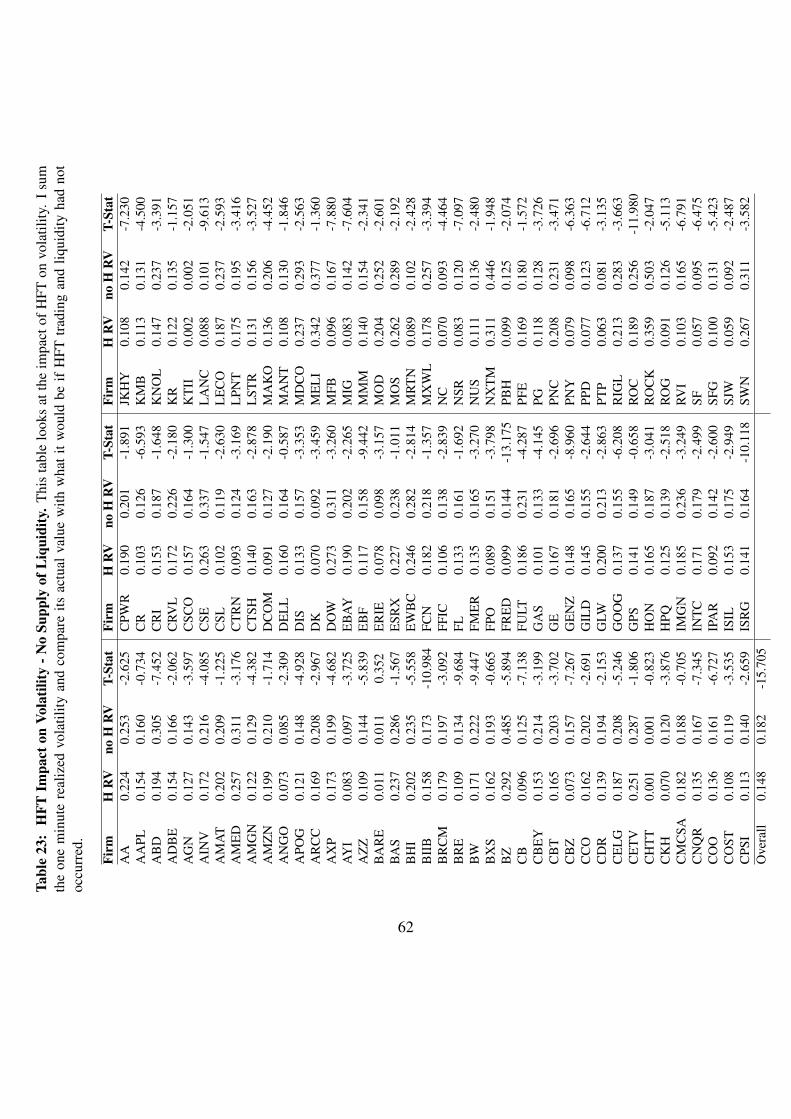
Tabl

e23

:H

FTIm

pact

onVo

latil

ity-N

oSu

pply

ofL

iqui

dity

.Thi

sta

ble

look

sat

the

impa

ctof

HFT

onvo

latil

ity.

Isu

mth

eon

em

inut

ere

aliz

edvo

latil

ityan

dco

mpa

reits

actu

alva

lue

with

wha

tit

wou

ldbe

ifH

FTtr

adin

gan

dliq

uidi

tyha

dno

toc

curr

ed.

Firm

HR

Vno

HR

VT-

Stat

Firm

HR

Vno

HR

VT-

Stat

Firm

HR

Vno

HR

VT-

Stat

AA

0.22

40.

253

-2.6

25C

PWR

0.19

00.

201

-1.8

91JK

HY

0.10

80.

142

-7.2

30A

APL

0.15

40.

160

-0.7

34C

R0.

103

0.12

6-6

.593

KM

B0.

113

0.13

1-4

.500

AB

D0.

194

0.30

5-7

.452

CR

I0.

153

0.18

7-1

.648

KN

OL

0.14

70.

237

-3.3

91A

DB

E0.

154

0.16

6-2

.062

CRV

L0.

172

0.22

6-2

.180

KR

0.12

20.

135

-1.1

57A

GN

0.12

70.

143

-3.5

97C

SCO

0.15

70.

164

-1.3

00K

TII

0.00

20.

002

-2.0

51A

INV

0.17

20.

216

-4.0

85C

SE0.

263

0.33

7-1

.547

LA

NC

0.08

80.

101

-9.6

13A

MA

T0.

202

0.20

9-1

.225

CSL

0.10

20.

119

-2.6

30L

EC

O0.

187

0.23

7-2

.593

AM

ED

0.25

70.

311

-3.1

76C

TR

N0.

093

0.12

4-3

.169

LPN

T0.

175

0.19

5-3

.416

AM

GN

0.12

20.

129

-4.3

82C

TSH

0.14

00.

163

-2.8

78L

STR

0.13

10.

156

-3.5

27A

MZ

N0.

199

0.21

0-1

.714

DC

OM

0.09

10.

127

-2.1

90M

AK

O0.

136

0.20

6-4

.452

AN

GO

0.07

30.

085

-2.3

09D

EL

L0.

160

0.16

4-0

.587

MA

NT

0.10

80.

130

-1.8

46A

POG

0.12

10.

148

-4.9

28D

IS0.

133

0.15

7-3

.353

MD

CO

0.23

70.

293

-2.5

63A

RC

C0.

169

0.20

8-2

.967

DK

0.07

00.

092

-3.4

59M

EL

I0.

342

0.37

7-1

.360

AX

P0.

173

0.19

9-4

.682

DO

W0.

273

0.31

1-3

.260

MFB

0.09

60.

167

-7.8

80A

YI

0.08

30.

097

-3.7

25E

BA

Y0.

190

0.20

2-2

.265

MIG

0.08

30.

142

-7.6

04A

ZZ

0.10

90.

144

-5.8

39E

BF

0.11

70.

158

-9.4

42M

MM

0.14

00.

154

-2.3

41B

AR

E0.

011

0.01

10.

352

ER

IE0.

078

0.09

8-3

.157

MO

D0.

204

0.25

2-2

.601

BA

S0.

237

0.28

6-1

.567

ESR

X0.

227

0.23

8-1

.011

MO

S0.

262

0.28

9-2

.192

BH

I0.

202

0.23

5-5

.558

EW

BC

0.24

60.

282

-2.8

14M

RT

N0.

089

0.10

2-2

.428

BII

B0.

158

0.17

3-1

0.98

4FC

N0.

182

0.21

8-1

.357

MX

WL

0.17

80.

257

-3.3

94B

RC

M0.

179

0.19

7-3

.092

FFIC

0.10

60.

138

-2.8

39N

C0.

070

0.09

3-4

.464

BR

E0.

109

0.13

4-9

.684

FL0.

133

0.16

1-1

.692

NSR

0.08

30.

120

-7.0

97B

W0.

171

0.22

2-9

.447

FME

R0.

135

0.16

5-3

.270

NU

S0.

111

0.13

6-2

.480

BX

S0.

162

0.19

3-0

.665

FPO

0.08

90.

151

-3.7

98N

XT

M0.

311

0.44

6-1

.948

BZ

0.29

20.

485

-5.8

94FR

ED

0.09

90.

144

-13.

175

PBH

0.09

90.

125

-2.0

74C

B0.

096

0.12

5-7

.138

FULT

0.18

60.

231

-4.2

87PF

E0.

169

0.18

0-1

.572

CB

EY

0.15

30.

214

-3.1

99G

AS

0.10

10.

133

-4.1

45PG

0.11

80.

128

-3.7

26C

BT

0.16

50.

203

-3.7

02G

E0.

167

0.18

1-2

.696

PNC

0.20

80.

231

-3.4

71C

BZ

0.07

30.

157

-7.2

67G

EN

Z0.

148

0.16

5-8

.960

PNY

0.07

90.

098

-6.3

63C

CO

0.16

20.

202

-2.6

91G

ILD

0.14

50.

155

-2.6

44PP

D0.

077

0.12

3-6

.712

CD

R0.

139

0.19

4-2

.153

GLW

0.20

00.

213

-2.8

63PT

P0.

063

0.08

1-3

.135

CE

LG

0.18

70.

208

-5.2

46G

OO

G0.

137

0.15

5-6

.208

RIG

L0.

213

0.28

3-3

.663

CE

TV

0.25

10.

287

-1.8

06G

PS0.

141

0.14

9-0

.658

RO

C0.

189

0.25

6-1

1.98

0C

HT

T0.

001

0.00

1-0

.823

HO

N0.

165

0.18

7-3

.041

RO

CK

0.35

90.

503

-2.0

47C

KH

0.07

00.

120

-3.8

76H

PQ0.

125

0.13

9-2

.518

RO

G0.

091

0.12

6-5

.113

CM

CSA

0.18

20.

188

-0.7

05IM

GN

0.18

50.

236

-3.2

49RV

I0.

103

0.16

5-6

.791

CN

QR

0.13

50.

167

-7.3

45IN

TC

0.17

10.

179

-2.4

99SF

0.05

70.

095

-6.4

75C

OO

0.13

60.

161

-6.7

27IP

AR

0.09

20.

142

-2.6

00SF

G0.

100

0.13

1-5

.423

CO

ST0.

108

0.11

9-3

.535

ISIL

0.15

30.

175

-2.9

49SJ

W0.

059

0.09

2-2

.487

CPS

I0.

113

0.14

0-2

.659

ISR

G0.

141

0.16

4-1

0.11

8SW

N0.

267

0.31

1-3

.582

Ove

rall

0.14

80.

182

-15.

705

62

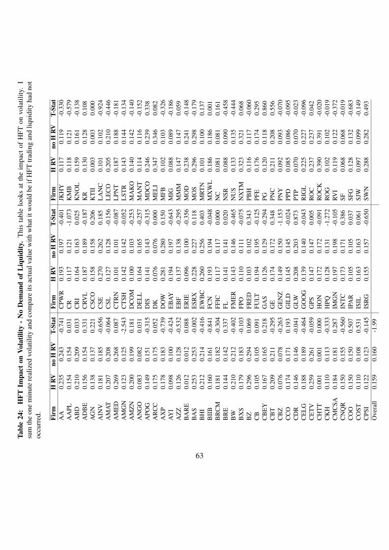
Tabl

e24

:H

FTIm

pact

onVo

latil

ity-

No

Dem

and

ofL

iqui

dity

.T

his

tabl

elo

oks

atth

eim

pact

ofH

FTon

vola

tility

.I

sum

the

one

min

ute

real

ized

vola

tility

and

com

pare

itsac

tual

valu

ew

ithw

hati

twou

ldbe

ifH

FTtr

adin

gan

dliq

uidi

tyha

dno

toc

curr

ed.

Firm

HR

Vno

HR

VT-

Stat

Firm

HR

Vno

HR

VT-

Stat

Firm

HR

Vno

HR

VT-

Stat

AA

0.23

50.

243

-0.7

41C

PWR

0.19

30.

197

-0.4

01JK

HY

0.11

70.

119

-0.3

30A

APL

0.15

40.

154

0.03

1C

R0.

117

0.12

1-1

.073

KM

B0.

118

0.12

1-0

.579

AB

D0.

210

0.20

90.

033

CR

I0.

164

0.16

30.

025

KN

OL

0.15

90.

161

-0.1

38A

DB

E0.

156

0.15

40.

331

CRV

L0.

187

0.18

9-0

.187

KR

0.13

00.

128

0.10

8A

GN

0.13

80.

137

0.22

1C

SCO

0.15

80.

158

0.20

6K

TII

0.00

30.

003

0.00

0A

INV

0.18

10.

185

-0.6

56C

SE0.

270

0.26

20.

185

LA

NC

0.10

10.

102

-0.9

24A

MA

T0.

207

0.20

8-0

.064

CSL

0.12

70.

128

-0.1

56L

EC

O0.

205

0.21

0-0

.446

AM

ED

0.26

90.

268

0.08

7C

TR

N0.

101

0.10

1-0

.087

LPN

T0.

187

0.18

8-0

.181

AM

GN

0.12

30.

125

-2.5

43C

TSH

0.14

20.

142

-0.0

52L

STR

0.14

30.

144

-0.1

34A

MZ

N0.

200

0.19

90.

181

DC

OM

0.10

00.

103

-0.2

53M

AK

O0.

140

0.14

2-0

.140

AN

GO

0.08

30.

082

0.03

1D

EL

L0.

164

0.16

5-0

.257

MA

NT

0.11

40.

116

-0.1

52A

POG

0.14

90.

151

-0.3

15D

IS0.

141

0.14

3-0

.315

MD

CO

0.24

60.

239

0.33

8A

RC

C0.

175

0.17

50.

052

DK

0.07

60.

076

0.00

0M

EL

I0.

347

0.34

60.

082

AX

P0.

178

0.18

3-0

.739

DO

W0.

281

0.28

00.

150

MFB

0.10

20.

103

-0.3

26A

YI

0.09

80.

100

-0.4

24E

BA

Y0.

194

0.19

7-0

.643

MIG

0.08

80.

089

-0.1

86A

ZZ

0.12

60.

128

-0.5

32E

BF

0.13

70.

138

-0.2

95M

MM

0.14

70.

147

0.05

9B

AR

E0.

012

0.01

20.

088

ER

IE0.

096

0.10

0-0

.356

MO

D0.

238

0.24

1-0

.148

BA

S0.

253

0.25

3-0

.002

ESR

X0.

228

0.22

70.

118

MO

S0.

296

0.29

8-0

.179

BH

I0.

212

0.21

4-0

.416

EW

BC

0.26

00.

256

0.40

3M

RT

N0.

101

0.10

00.

137

BII

B0.

160

0.16

1-0

.841

FCN

0.19

30.

194

-0.0

48M

XW

L0.

186

0.18

60.

001

BR

CM

0.18

10.

182

-0.3

04FF

IC0.

117

0.11

70.

000

NC

0.08

10.

081

0.16

1B

RE

0.14

40.

142

0.33

7FL

0.14

10.

141

0.02

0N

SR0.

088

0.09

0-0

.458

BW

0.21

00.

212

-0.4

02FM

ER

0.14

30.

146

-0.4

65N

US

0.13

30.

135

-0.4

44B

XS

0.17

90.

183

-0.1

03FP

O0.

110

0.11

1-0

.075

NX

TM

0.32

30.

321

0.06

8B

Z0.

296

0.29

40.

069

FRE

D0.

103

0.10

20.

343

PBH

0.11

60.

117

-0.0

60C

B0.

105

0.10

50.

091

FULT

0.19

40.

195

-0.1

25PF

E0.

176

0.17

40.

295

CB

EY

0.16

70.

165

0.21

8G

AS

0.12

60.

129

-0.2

94PG

0.12

00.

118

0.86

0C

BT

0.20

90.

211

-0.2

95G

E0.

174

0.17

20.

348

PNC

0.21

10.

208

0.55

6C

BZ

0.07

60.

078

-0.2

63G

EN

Z0.

149

0.15

0-1

.153

PNY

0.09

20.

093

-0.0

70C

CO

0.17

40.

171

0.19

3G

ILD

0.14

50.

145

-0.0

24PP

D0.

085

0.08

6-0

.095

CD

R0.

146

0.14

6-0

.041

GLW

0.20

80.

203

0.87

3PT

P0.

070

0.07

0-0

.023

CE

LG

0.18

80.

189

-0.4

64G

OO

G0.

139

0.14

0-0

.043

RIG

L0.

225

0.22

7-0

.096

CE

TV

0.25

90.

261

-0.0

59G

PS0.

147

0.14

70.

005

RO

C0.

237

0.23

70.

042

CH

TT

0.00

10.

001

0.00

0H

ON

0.17

20.

172

-0.0

91R

OC

K0.

390

0.39

1-0

.020

CK

H0.

110

0.11

3-0

.333

HPQ

0.12

80.

131

-1.2

72R

OG

0.10

20.

102

-0.0

19C

MC

SA0.

184

0.18

10.

287

IMG

N0.

197

0.19

8-0

.105

RVI

0.11

90.

122

-0.3

72C

NQ

R0.

150

0.15

5-0

.560

INT

C0.

173

0.17

10.

386

SF0.

068

0.06

8-0

.019

CO

O0.

150

0.15

00.

507

IPA

R0.

105

0.10

50.

037

SFG

0.12

80.

132

-0.6

83C

OST

0.11

00.

108

0.53

1IS

IL0.

163

0.16

30.

061

SJW

0.09

70.

099

-0.1

49C

PSI

0.12

20.

123

-0.1

45IS

RG

0.15

50.

157

-0.6

50SW

N0.

288

0.28

20.

493

Ove

rall

0.15

90.

160

-1.9

9

63

7 ConclusionThis paper examines high frequency trading and its role in financial markets. HFTmake up a large majority of all trades. They supply liquidity in about half of alltrades and demand liquidity in about half as well. Their activities i nthe market,both in initiating trades and in providing liqidity, are stable over time. They tendto engage in a price reversal strategy, and this is stronger when they are demand-ing liquidity. There is no evidence of abusive front running occurring. The HFTfirms are profitable, making around $3 billion between the 26 of them. HFT preferto trade in large stocks with lower volume, lower spreads and depth, and compa-nies that are considered value firms. They tend to make more money in volatiletimes. HFT prefer to demand liquidity in small amounts, usually in value between$1,000 and $4,999, and they tend to have lower time between trades than non-HFT. They provide the best quotes about 45% of the time. They provide moreinside quotes for larger value firms, with lower volume, lower volatility, lowerspreads and depth, and with greater number of trades. From the different Has-brouck measures, the evidence suggest HFT play a very important role in priceefficiency and the price discovery process. In fact, they provide more useful in-formation to the price generation process than do non-HFT. Finally, HFT activityeither has no impact on volatility or tends to decrease it.

64

ReferencesM.J. Barclay, T. Hendershott, and D.T. McCormick. Competition among trad-

ing venues: Information and trading on electronic communications networks.Journal of Finance, 58(6):2637–2665, 2003.

B. Biais, P. Hillion, and C. Spatt. An empirical analysis of the limit order bookand the order flow in the Paris Bourse. Journal of Finance, 50(5):1655–1689,1995.

A. Chaboud, E. Hjalmarsson, C. Vega, and B. Chiquoine. Rise of the machines:Algorithmic trading in the foreign exchange market. International FinanceDiscussion Papers, 2009.

J. Creswell. Speedy New Traders Make Waves Far From Wall Street. New YorkTimes, (http://www.nytimes.com/2010/05/17/business/17trade.html?dbk), May16, 2010.

T. Foucault and A.J. Menkveld. Competition for order flow and smart order rout-ing systems. The Journal of Finance, 63(1):119–158, 2008.

K.A. Froot, D.S. Scharfstein, and J.C. Stein. Herd on the street: Informationalinefficiencies in a market with short-term speculation. Journal of finance, 47(4):1461–1484, 1992.

J. Hasbrouck. Measuring the information content of stock trades. Journal ofFinance, 46(1):179–207, 1991a.

J. Hasbrouck. The summary informativeness of stock trades: An econometricanalysis. Review of Financial Studies, 4(3):571–595, 1991b.

J. Hasbrouck. One security, many markets: Determining the contributions to pricediscovery. Journal of Finance, pages 1175–1199, 1995.

J.A. Hausman, A.W. Lo, and A.C. MacKinlay. An ordered probit analysis oftransaction stock prices. Journal of financial economics, 31(3):319–379, 1992.

T. Hendershott and P.C. Moulton. Speed and stock market quality: The NYSEsHybrid. Manuscript, UC Berkeley, 2007.

T. Hendershott and R. Riordan. Algorithmic trading and information. SSRN, 2009.

65

T. Hendershott, C.M. Jones, and A.J. Menkveld. Does Algorithmic Trading Im-prove Liquidity? Journal of Finance, Forthcoming, 2008.

M. Kearns, A. Kulesza, and Y. Nevmyvaka. Empirical Limitations on High Fre-quency Trading Profitability. Unpublished, 2010.

E. Krudy. Is the May 6 ”flash crash” in US stock markets the new normal?Reuters, (http://www.reuters.com/article/idUSN1057063420100610), June 10,2010.

Securities and Exchange Commission. Concept Release on Equity Market Struc-ture. (Concept Release on Equity Market Structure), January 14, 2010.

Lash H. Spicer, J. Who’s afraid of high-frequency trading. Reuters,(http://www.reuters.com/article/idUSN173583920091202), December 2, 2009.

X. Vives. Short-term investment and the informational efficiency of the market.Review of Financial Studies, 8(1):125–160, 1995.

66