HIGH-FREQUENCY TURBULENCE AND SEDIMENT FLUX MEASUREMENTS IN AN UPPER ESTUARINE ZONE

Hubert CHANSON, Mark TREVETHAN, and Maiko TAKEUCHI Div. of Civil Engineering, The University of Queensland, Brisbane QLD 4072, Australia

Ph.: (61 7) 3365 4163 - Fax: (61 7) 3365 4599 - E-mail: h.chanson@uq.edu.au Abstract : In natural estuaries, the predictions of scalar dispersion are rarely predicted accurately because of a lack of fundamental understanding of the turbulence structure in estuaries. Herein detailed turbulence field measurements were conducted continuously at high frequency for 50 hours in the upper zone of a small subtropical estuary with semi-diurnal tides. Acoustic Doppler velocimetry was deemed the most appropriate measurement technique for such shallow water depths (less than 0.4 m at low tides), and a thorough post-processing technique was applied. In addition, some experiments were conducted in laboratory under controlled conditions using water and soil samples collected in the estuary to test the relationship between acoustic backscatter strength and suspended sediment load. A striking feature of the field data set was the large fluctuations in all turbulence characteristics during the tidal cycle, including the suspended sediment flux. This feature was rarely documented. Keywords : Turbulence measurements, Suspended sediment concentration, Subtropical estuary, Continuous high-frequency sampling, Acoustic backscatter.

INTRODUCTION In natural estuaries, the prediction of scalar dispersion in estuaries can rarely be predicted

analytically without exhaustive field data for calibration and validation. Why is it? In natural estuaries, the flow Reynolds number is typically within the range of 1 E+5 to 1 E+8 and more. That is, the flow is turbulent, and we lack some fundamental understanding of the turbulence structure in estuaries. In addition, a few studies investigated the lower and middle estuary but the upper/upstream estuary dynamics received little attention.

The purpose of this study is to investigate thoroughly the turbulence and sediment suspension characteristics in the upper estuary zone of a small subtropical system. Detailed field measurements were conducted continuously at high frequency in a small estuary with semi-diurnal tides. Laboratory experiments were conducted under controlled conditions using the estuary water and soil samples to validate the monotonic relationship between acoustic backscatter strength, turbidity and suspended sediment load. The results yielded an unique series of high-frequency long duration (50 Hz, 50 hours) measurements of turbulent velocity and suspended sediment concentration SSC in the upper estuary.

TURBULENCE CHARACTERISTICS Turbulent flows have a great mixing potential involving a wide range of eddy length scales.

Although the turbulence is a "random" process, the small departures from a Gaussian probability distribution are some key features of turbulence. For example, the skewness and kurtosis give some information on the temporal distribution of the turbulent velocity fluctuation around its mean value. A non-zero skewness indicates some degree of temporal asymmetry of the turbulent fluctuation (e.g. acceleration versus deceleration, sweep versus ejection). The skewness retains some sign information and it can be used to extract basic information without ambiguity. An excess kurtosis larger than zero is associated with a peaky signal: e.g., produced by intermittent turbulent events.

In turbulence studies, the measured statistics include usually (a) the spatial distribution of Reynolds stresses, (b) the rates at which the individual Reynolds stresses are produced, destroyed or transported from one point in space to another, (c) the contribution of different sizes of eddy to the Reynolds stresses, and (d) the contribution of different sizes of eddy to the rates mentioned in (b) and to rate at which Reynolds stresses are transferred from one range of eddy size to another (BRADSHAW 1971). The Reynolds stress is a transport effect resulting from turbulent motion induced by velocity fluctuations with its subsequent increase of momentum exchange and of mixing (PIQUET 1999). The turbulent transport is a property of the flow. The turbulent stress tensor, or Reynolds stress tensor, includes the normal and tangential stresses, although there is no fundamental

difference between normal stress and tangential stress. For example, (vx+vy)/ 2 is the component of the velocity fluctuation along a line in the xy-plane at 45º to the x-axis; hence its mean square

2/)vv2vv( yx2

y2

x ××++ is the component of the normal stress over the density in this direction although it is a combination of normal and tangential stresses in the x- and y-axes.

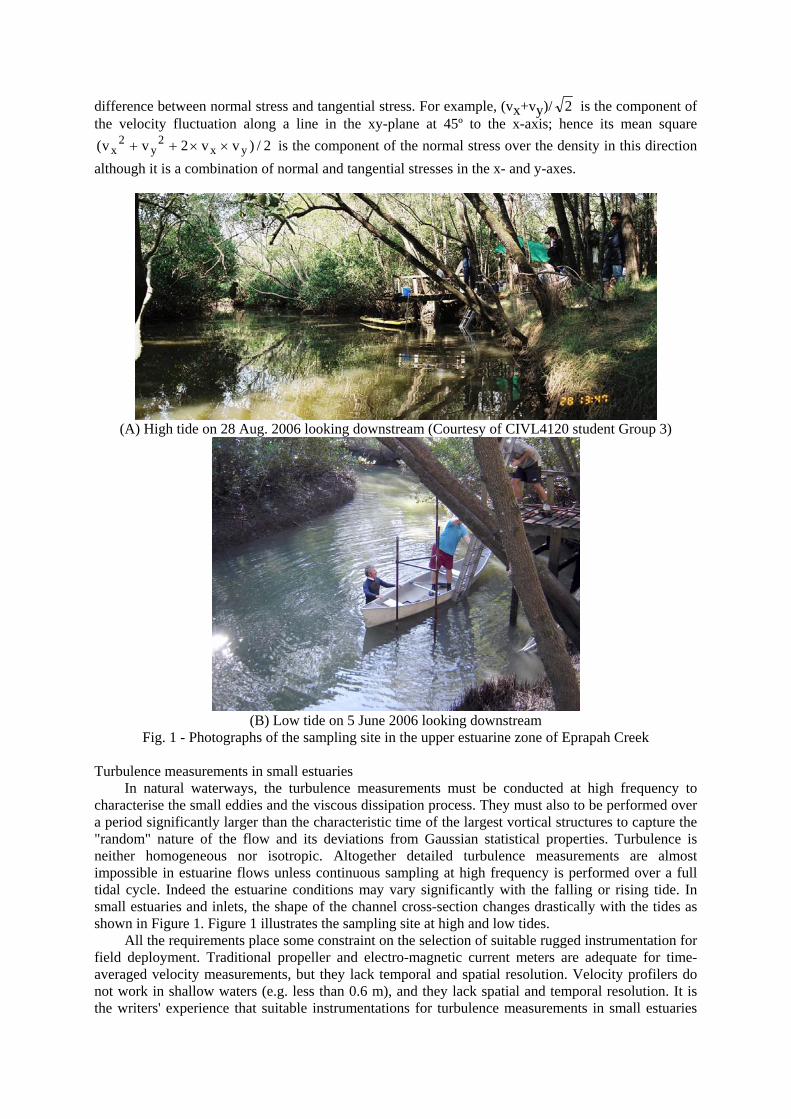
(A) High tide on 28 Aug. 2006 looking downstream (Courtesy of CIVL4120 student Group 3)

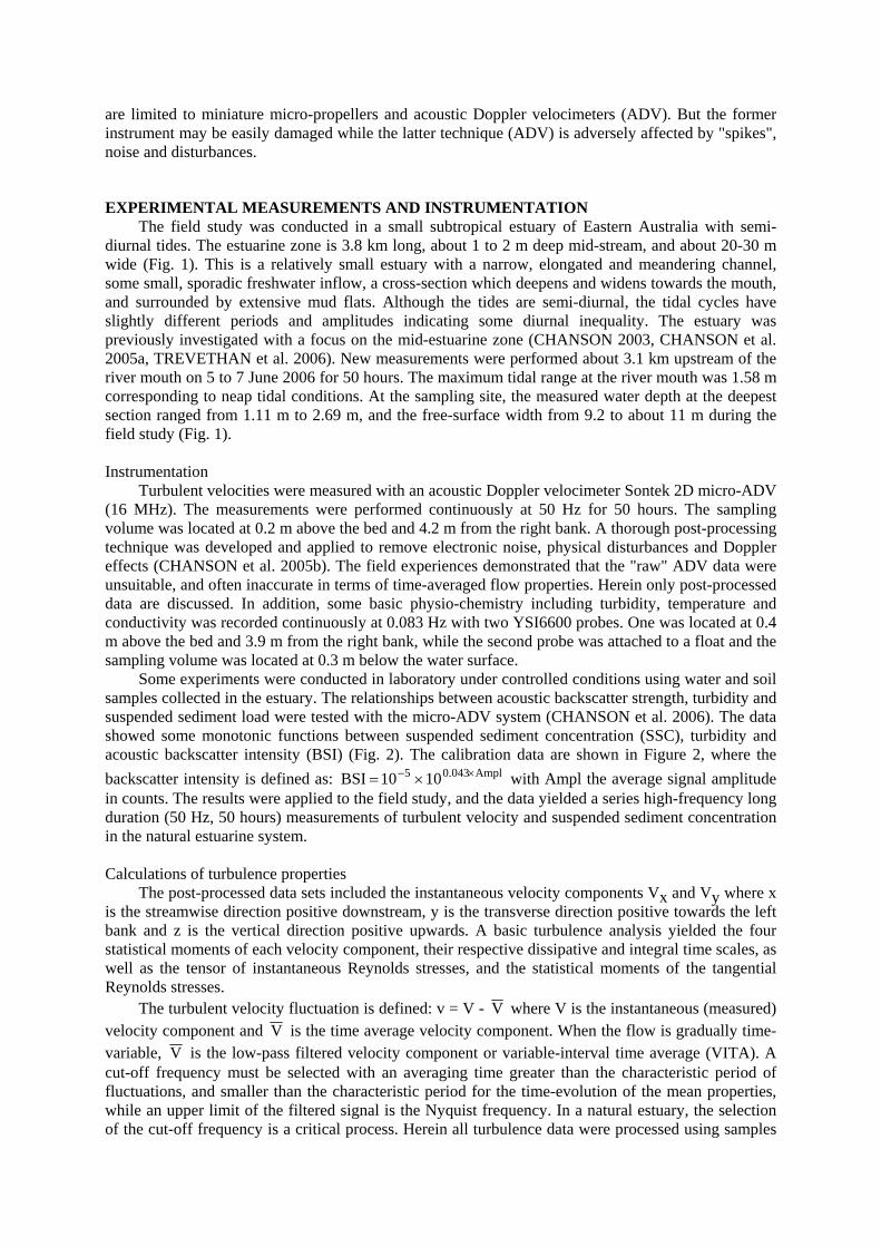
(B) Low tide on 5 June 2006 looking downstream

Fig. 1 - Photographs of the sampling site in the upper estuarine zone of Eprapah Creek Turbulence measurements in small estuaries

In natural waterways, the turbulence measurements must be conducted at high frequency to characterise the small eddies and the viscous dissipation process. They must also to be performed over a period significantly larger than the characteristic time of the largest vortical structures to capture the "random" nature of the flow and its deviations from Gaussian statistical properties. Turbulence is neither homogeneous nor isotropic. Altogether detailed turbulence measurements are almost impossible in estuarine flows unless continuous sampling at high frequency is performed over a full tidal cycle. Indeed the estuarine conditions may vary significantly with the falling or rising tide. In small estuaries and inlets, the shape of the channel cross-section changes drastically with the tides as shown in Figure 1. Figure 1 illustrates the sampling site at high and low tides.

All the requirements place some constraint on the selection of suitable rugged instrumentation for field deployment. Traditional propeller and electro-magnetic current meters are adequate for time-averaged velocity measurements, but they lack temporal and spatial resolution. Velocity profilers do not work in shallow waters (e.g. less than 0.6 m), and they lack spatial and temporal resolution. It is the writers' experience that suitable instrumentations for turbulence measurements in small estuaries

are limited to miniature micro-propellers and acoustic Doppler velocimeters (ADV). But the former instrument may be easily damaged while the latter technique (ADV) is adversely affected by "spikes", noise and disturbances.

EXPERIMENTAL MEASUREMENTS AND INSTRUMENTATION The field study was conducted in a small subtropical estuary of Eastern Australia with semi-

diurnal tides. The estuarine zone is 3.8 km long, about 1 to 2 m deep mid-stream, and about 20-30 m wide (Fig. 1). This is a relatively small estuary with a narrow, elongated and meandering channel, some small, sporadic freshwater inflow, a cross-section which deepens and widens towards the mouth, and surrounded by extensive mud flats. Although the tides are semi-diurnal, the tidal cycles have slightly different periods and amplitudes indicating some diurnal inequality. The estuary was previously investigated with a focus on the mid-estuarine zone (CHANSON 2003, CHANSON et al. 2005a, TREVETHAN et al. 2006). New measurements were performed about 3.1 km upstream of the river mouth on 5 to 7 June 2006 for 50 hours. The maximum tidal range at the river mouth was 1.58 m corresponding to neap tidal conditions. At the sampling site, the measured water depth at the deepest section ranged from 1.11 m to 2.69 m, and the free-surface width from 9.2 to about 11 m during the field study (Fig. 1). Instrumentation

Turbulent velocities were measured with an acoustic Doppler velocimeter Sontek 2D micro-ADV (16 MHz). The measurements were performed continuously at 50 Hz for 50 hours. The sampling volume was located at 0.2 m above the bed and 4.2 m from the right bank. A thorough post-processing technique was developed and applied to remove electronic noise, physical disturbances and Doppler effects (CHANSON et al. 2005b). The field experiences demonstrated that the "raw" ADV data were unsuitable, and often inaccurate in terms of time-averaged flow properties. Herein only post-processed data are discussed. In addition, some basic physio-chemistry including turbidity, temperature and conductivity was recorded continuously at 0.083 Hz with two YSI6600 probes. One was located at 0.4 m above the bed and 3.9 m from the right bank, while the second probe was attached to a float and the sampling volume was located at 0.3 m below the water surface.

Some experiments were conducted in laboratory under controlled conditions using water and soil samples collected in the estuary. The relationships between acoustic backscatter strength, turbidity and suspended sediment load were tested with the micro-ADV system (CHANSON et al. 2006). The data showed some monotonic functions between suspended sediment concentration (SSC), turbidity and acoustic backscatter intensity (BSI) (Fig. 2). The calibration data are shown in Figure 2, where the backscatter intensity is defined as: Ampl043.05 1010BSI ×− ×= with Ampl the average signal amplitude in counts. The results were applied to the field study, and the data yielded a series high-frequency long duration (50 Hz, 50 hours) measurements of turbulent velocity and suspended sediment concentration in the natural estuarine system. Calculations of turbulence properties

The post-processed data sets included the instantaneous velocity components Vx and Vy where x is the streamwise direction positive downstream, y is the transverse direction positive towards the left bank and z is the vertical direction positive upwards. A basic turbulence analysis yielded the four statistical moments of each velocity component, their respective dissipative and integral time scales, as well as the tensor of instantaneous Reynolds stresses, and the statistical moments of the tangential Reynolds stresses.

The turbulent velocity fluctuation is defined: v = V - V where V is the instantaneous (measured) velocity component and V is the time average velocity component. When the flow is gradually time-variable, V is the low-pass filtered velocity component or variable-interval time average (VITA). A cut-off frequency must be selected with an averaging time greater than the characteristic period of fluctuations, and smaller than the characteristic period for the time-evolution of the mean properties, while an upper limit of the filtered signal is the Nyquist frequency. In a natural estuary, the selection of the cut-off frequency is a critical process. Herein all turbulence data were processed using samples

that contain 10,000 data points (200 s) and calculated every 10 s along the entire data sets. The sample size (200 s) was deduced from a sensitivity analysis. It was chosen to be much larger than the instantaneous velocity fluctuation time scales, to contain enough data points to yield statistically meaningful results, and to be considerably smaller than the period of tidal fluctuations. In a study of boundary layer flows, FRANSSON et al. (2005) proposed a cut-off frequency that is consistent with the selected sample size.

Acoustic backscatter intensity BSI

Susp

ende

d se

dim

ent c

once

ntra

tion

SSC

(kg/

m3 )

Turb

idity

(NTU

)

0 2 4 6 8 10 12 140 0

0.2 40

0.4 80

0.6 120

0.8 160

Eprapah waters, Bed sample 1CHANSON et al. (2006)

SSC dataTurbidity dataSSC = 0.9426 * (1 - exp(-0.1109 * BSI))Turbidity = 171.1 * (1 - exp(-0.1593 * x))

Fig. 2 - Relationships between suspended sediment concentration, turbidity and acoustic backscatter

intensity for the Sontek 2D micro-ADV (A641F) at Eprapah Creek

Fig. 3 - Velocity auto-correlation function and turbulent time scale definitions

An auto-correlation analysis yields further the Eulerian dissipation and integral time scales for

each velocity component (Fig. 3). The integral time scale, or Taylor macro scale, is a rough measure of the longest connection in the turbulent behaviour of a velocity component. The dissipation time scale τE represents a measure of the most rapid changes that occur in the fluctuations of a velocity component, and it is the smallest energetic time scale. Herein τE was calculated using the method of HALLBACK et al. (1989) extended by FRANSSON et al. (2005) and KOCH and CHANSON (2005).

The Reynolds stress tensor includes the normal and tangential stresses. Each instantaneous Reynolds stress (e.g. yx vv ××ρ ) is characterised by its four statistical moments : i.e., the time-

averaged stress, its standard deviation, skewness and kurtosis, where ρ is the fluid density. Lastly the turbulence calculations were not conducted when more than 20% of the 10,000 data

points were corrupted/repaired during the ADV data post-processing.

Time (s) since 00:00 on 5/6/2006

Dep

th (m

)

Con

duct

ivity

(mS/

cm)

40000 60000 80000 100000 120000 140000 160000 180000 200000 2200000.9 24

1.1 28

1.3 32

1.5 36

1.7 40

1.9 44

2.1 48

2.3 52

2.5 56

2.7 60Water depth (m)Conductivity at 0.4 m above bed (mS/cm)Conductivity at 0.3 m below surface (mS/cm)

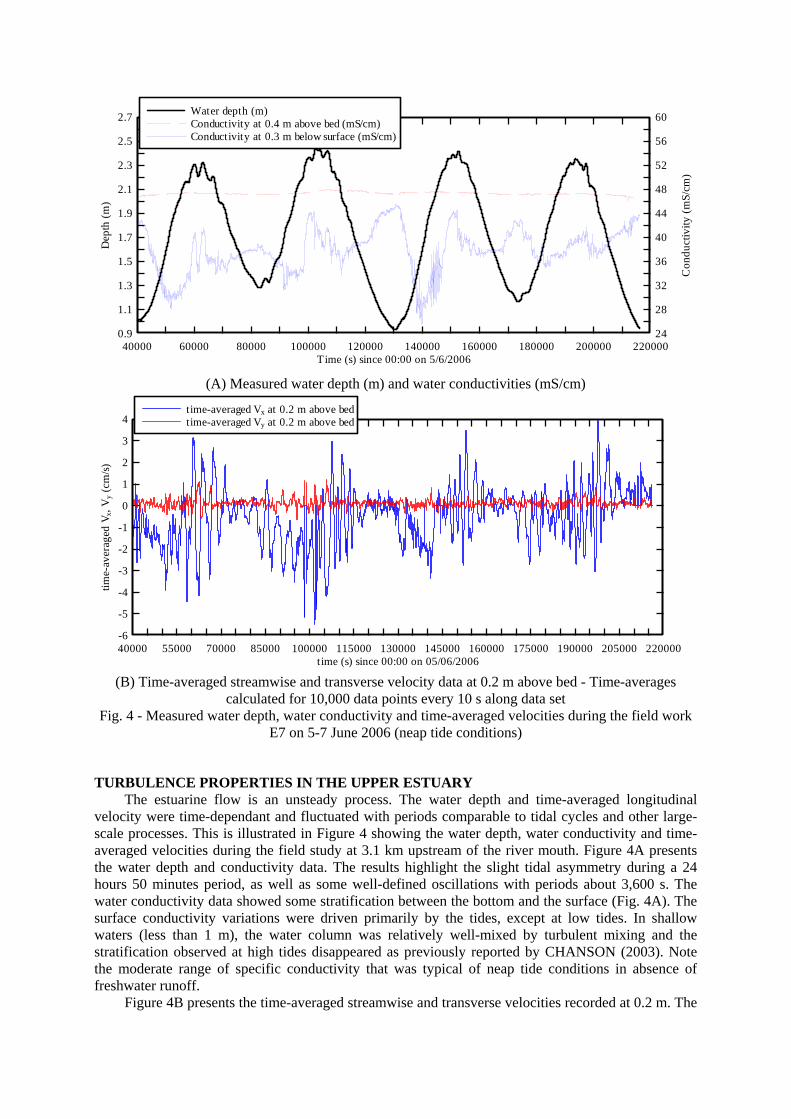
(A) Measured water depth (m) and water conductivities (mS/cm)

time (s) since 00:00 on 05/06/2006

time-

aver

aged

Vx,

Vy (

cm/s)

40000 55000 70000 85000 100000 115000 130000 145000 160000 175000 190000 205000 220000-6

-5

-4

-3

-2

-1

0

1

2

3

4time-averaged Vx at 0.2 m above bedtime-averaged Vy at 0.2 m above bed

(B) Time-averaged streamwise and transverse velocity data at 0.2 m above bed - Time-averages

calculated for 10,000 data points every 10 s along data set Fig. 4 - Measured water depth, water conductivity and time-averaged velocities during the field work

E7 on 5-7 June 2006 (neap tide conditions)

TURBULENCE PROPERTIES IN THE UPPER ESTUARY The estuarine flow is an unsteady process. The water depth and time-averaged longitudinal

velocity were time-dependant and fluctuated with periods comparable to tidal cycles and other large-scale processes. This is illustrated in Figure 4 showing the water depth, water conductivity and time-averaged velocities during the field study at 3.1 km upstream of the river mouth. Figure 4A presents the water depth and conductivity data. The results highlight the slight tidal asymmetry during a 24 hours 50 minutes period, as well as some well-defined oscillations with periods about 3,600 s. The water conductivity data showed some stratification between the bottom and the surface (Fig. 4A). The surface conductivity variations were driven primarily by the tides, except at low tides. In shallow waters (less than 1 m), the water column was relatively well-mixed by turbulent mixing and the stratification observed at high tides disappeared as previously reported by CHANSON (2003). Note the moderate range of specific conductivity that was typical of neap tide conditions in absence of freshwater runoff.

Figure 4B presents the time-averaged streamwise and transverse velocities recorded at 0.2 m. The

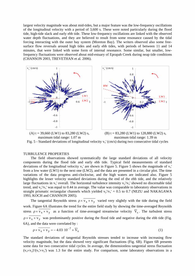
largest velocity magnitude was about mid-tides, but a major feature was the low-frequency oscillations of the longitudinal velocity with a period of 3,600 s. These were noted particularly during the flood tide, high-tide slack and early ebb tide. These low-frequency oscillations are linked with the observed water depth fluctuations, and they are believed to result from some resonance caused by the tidal forcing interacting with the outer bay system (Moreton Bay). The writers observed also some free-surface flow reversals around high tides and early ebb tides, with periods of between 11 and 14 minutes, that were linked with some form of internal resonance. Some similar, but smaller, low-frequency fluctuations were observed about mid-estuary of Eprapah Creek during neap tide conditions (CHANSON 2003, TREVETHAN et al. 2006).

-1

-0.8

-0.6

-0.4

-0.2

0

0.2

0.4

0.6

0.8

1

-1 -0.6 -0.2 0.2 0.6 1

LW1

HW LW2

vx' (cm/s)

-1

-0.8

-0.6

-0.4

-0.2

0

0.2

0.4

0.6

0.8

1

-1 -0.6 -0.2 0.2 0.6 1

LW1

LW2

HW

vx' (cm/s)

(A) t = 39,660 (LW1) to 83,280 (LW2) s,

maximum tidal range: 1.07 m (B) t = 83,280 (LW1) to 128,880 (LW2) s,

maximum tidal range: 1.39 m Fig. 5 - Standard deviations of longitudinal velocity vx' (cm/s) during two consecutive tidal cycles

TURBULENCE PROPERTIES The field observations showed systematically the large standard deviations of all velocity

components during the flood tide and early ebb tide. Typical field measurements of standard deviations of the longitudinal velocity vx' are shown in Figure 5. Figure 5 shows the magnitude of vx' from a low water (LW1) to the next one (LW2), and the data are presented in a circular plot. The time variations of the data progress anti-clockwise, and the high waters are indicated also. Figure 5 highlights the lesser velocity standard deviations during the end of the ebb tide, and the relatively large fluctuations in vx' overall. The horizontal turbulence intensity vy'/vx' showed no discernable tidal trend, and vy'/vx' was equal to 0.44 in average. The value was comparable to laboratory observations in straight prismatic rectangular channels which yielded vy'/vx' = 0.5 to 0.7 (NEZU and NAKAGAWA 1993, KOCH and CHANSON 2005).

The tangential Reynolds stress yx vv ××ρ varied very slightly with the tide during the field work. Figure 6A illustrates the trend for the entire field study by showing the time-averaged Reynolds stress yx vv ××ρ as a function of time-averaged streamwise velocity xV . The turbulent stress

yx vv ××ρ was predominantly positive during the flood tide and negative during the ebb tide (Fig. 6A), and the data were correlated by :

x7

yx V1003.4vv ×−=××ρ − (1)

The standard deviations of tangential Reynolds stresses tended to increase with increasing flow velocity magnitude, but the data showed very significant fluctuations (Fig. 6B). Figure 6B presents some data for two consecutive tidal cycles. In average, the dimensionless tangential stress fluctuation (vx×vy)'/(vx'×vy') was 1.3 for the entire study. For comparison, some laboratory observations in a

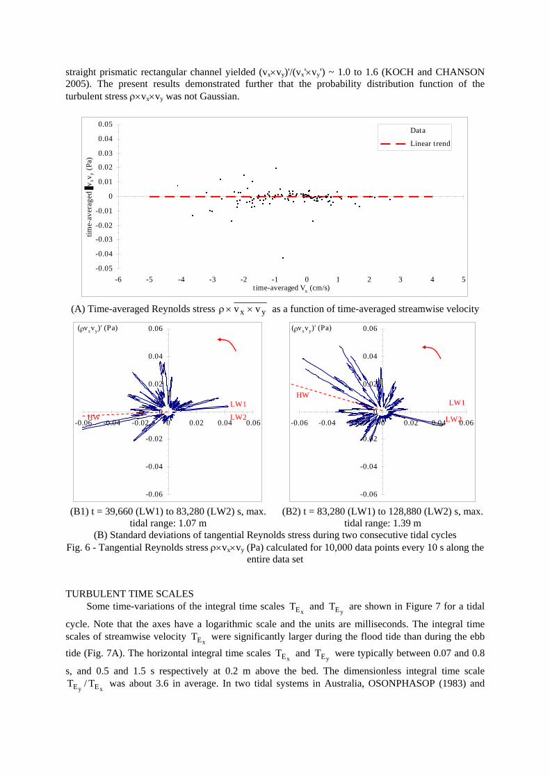
straight prismatic rectangular channel yielded (vx×vy)'/(vx'×vy') ~ 1.0 to 1.6 (KOCH and CHANSON 2005). The present results demonstrated further that the probability distribution function of the turbulent stress ρ×vx×vy was not Gaussian.

-0.05

-0.04

-0.03

-0.02

-0.01

0

0.01

0.02

0.03

0.04

0.05

-6 -5 -4 -3 -2 -1 0 1 2 3 4 5time-averaged Vx (cm/s)

time-

aver

aged

vxv

y (Pa

)

Data

Linear trend

(A) Time-averaged Reynolds stress yx vv ××ρ as a function of time-averaged streamwise velocity

-0.06

-0.04

-0.02

0

0.02

0.04

0.06

-0.06 -0.04 -0.02 0 0.02 0.04 0.06

LW1

LW2HW

(ρvxvy)' (Pa)

-0.06

-0.04

-0.02

0

0.02

0.04

0.06

-0.06 -0.04 -0.02 0 0.02 0.04 0.06

LW1

LW2

HW

(ρvxvy)' (Pa)

(B1) t = 39,660 (LW1) to 83,280 (LW2) s, max.

tidal range: 1.07 m (B2) t = 83,280 (LW1) to 128,880 (LW2) s, max.

tidal range: 1.39 m (B) Standard deviations of tangential Reynolds stress during two consecutive tidal cycles

Fig. 6 - Tangential Reynolds stress ρ×vx×vy (Pa) calculated for 10,000 data points every 10 s along the entire data set

TURBULENT TIME SCALES Some time-variations of the integral time scales

xET and yET are shown in Figure 7 for a tidal

cycle. Note that the axes have a logarithmic scale and the units are milliseconds. The integral time scales of streamwise velocity

xET were significantly larger during the flood tide than during the ebb tide (Fig. 7A). The horizontal integral time scales

xET and yET were typically between 0.07 and 0.8

s, and 0.5 and 1.5 s respectively at 0.2 m above the bed. The dimensionless integral time scale

yET /xET was about 3.6 in average. In two tidal systems in Australia, OSONPHASOP (1983) and

TREVETHAN et al. (2006) observed respectively yET /

xET ~ 1.7 and 1.0, while KOCH and

CHANSON (2005) observed yET /

xET ~ 0.4 in a laboratory channel.

The turbulent dissipation time scale, or Taylor micro-scale, is a characteristic time scale of the smaller eddies which are primary responsible for the dissipation of energy. The data yielded dissipation time scales of about 1 ms in average, with most data between 0.4 and 3 ms. Such dissipation time scales were smaller than the time between two consecutive samples: e.g., 1/Fscan = 0.02 s for Fscan = 50 Hz. The findings highlighted that a high-frequency sampling is required and the sampling rates must be at least 50 Hz to capture a range of eddy time scales relevant to the dissipation processes. The analysis of dissipation time scales of all velocity components showed no obvious trend with the tidal phase (Fig. 8). The dimensionless transverse dissipation time scale was about

yEτ /xEτ

~ 1.9. KOCH and CHANSON (2005) obtained yEτ /

xEτ ~ 0.9 in a rectangular channel. Some

estimate of integral length scales may be derived using Taylor's hypothesis: Exf TV ×=Λ . The integral scale Λf is a measure of the longest connection between the velocities at two points of the flow field (HINZE 1975). Herein the horizontal integral length scales were between 0.2 and 3 cm.

-4

-3

-2

-1

0

1

2

3

4

-4 -3 -2 -1 0 1 2 3 4

LW1

LW2HW

log10T Ex (ms)

-4

-3

-2

-1

0

1

2

3

4

-4 -3 -2 -1 0 1 2 3 4

LW1

LW2HW

log10T Ey (ms)

(A) Longitudinal integral time scales

xET (B) Transverse integral time scales yET

Fig. 7 - Integral turbulent time scales (units: ms) for t = 39,660 (LW1) to 83,280 (LW2) s

-5

-3

-1

1

3

5

-5 -3 -1 1 3 5

LW1

LW2HW

log10 τEx (µs)

-5

-3

-1

1

3

5

-5 -3 -1 1 3 5

LW1

LW2HW

log10 τEy (µs)

(A)

xEτ (B) yEτ

Fig. 8 - Turbulent dissipation time scales (units: µs) for t = 39,660 (LW1) to 83,280 (LW2) s

SUSPENDED SEDIMENT FLUX High-frequency suspended sediment concentration data were deduced from the ADV backscatter

signal. The instantaneous advective suspended sediment flux per unit area qs was calculated as :

xs VSSCq ×= (6)

where qs and Vx are positive in the downstream direction, and SSC is the suspended sediment concentration SSC is in kg/m3. The results are presented in Figure 9. The sediment flux data showed typically an upstream, negative suspended sediment flux during the flood tide and a downstream, positive sediment flux during the ebb tide. The instantaneous sediment flux data qs showed considerable time-fluctuations that derived from a combination of velocity and suspended sediment concentration fluctuations. The data demonstrated further some high-frequency fluctuation with some form of sediment flux bursts that were likely linked to and caused by some turbulent bursting phenomena next to the bed (e.g. JACKSON 1976). Some low-frequency fluctuations in sediment flux were also observed.

The sediment flux data were integrated with respect of time. The result gave the net sediment mass transfer per unit area during a full tidal cycle. For the entire field study, the net sediment mass transfer per area was negative and yielded -4.2 kg/m2 on average. The net sediment flux was upstream.

Time (s) since 00:00 on 5/6/2006

SSC×V

x (kg

/s/m

2 )

Wat

er d

epth

(m)

40000 60000 80000 100000 120000 140000 160000 180000 200000 220000-0.002 0.6

-0.0016 0.8

-0.0012 1

-0.0008 1.2

-0.0004 1.4

0 1.6

0.0004 1.8

0.0008 2

0.0012 2.2

0.0016 2.4

0.002 2.6

40000 60000 80000 100000 120000 140000 160000 180000 200000 220000-0.002 0.6

-0.0016 0.8

-0.0012 1

-0.0008 1.2

-0.0004 1.4

0 1.6

0.0004 1.8

0.0008 2

0.0012 2.2

0.0016 2.4

0.002 2.6SSC×V x (kg/s/m2)Water depth (m)

Fig. 9 - Time variations of suspended sediment flux per unit surface area (SSC×Vx), positive

downstream, and measured water depth for the 50 hours study period

CONCLUSIONS In natural estuaries, the suspended sediment processes are driven by the turbulent momentum

mixing. The predictions of scalar dispersion can rarely be predicted accurately because of a lack of fundamental understanding of the turbulence structure in estuaries. Herein detailed turbulence and suspended sediment field measurements were conducted continuously at high frequency in a small subtropical estuary with semi-diurnal tides. The study was focused on the upper estuarine region of an elongated system.

The data set demonstrated some unique features of the upstream estuary, in particular some low-frequency longitudinal flow oscillations induced by internal and outer resonance. These long-period oscillations induced fluctuations in turbulent velocity and suspended sediment flux that were

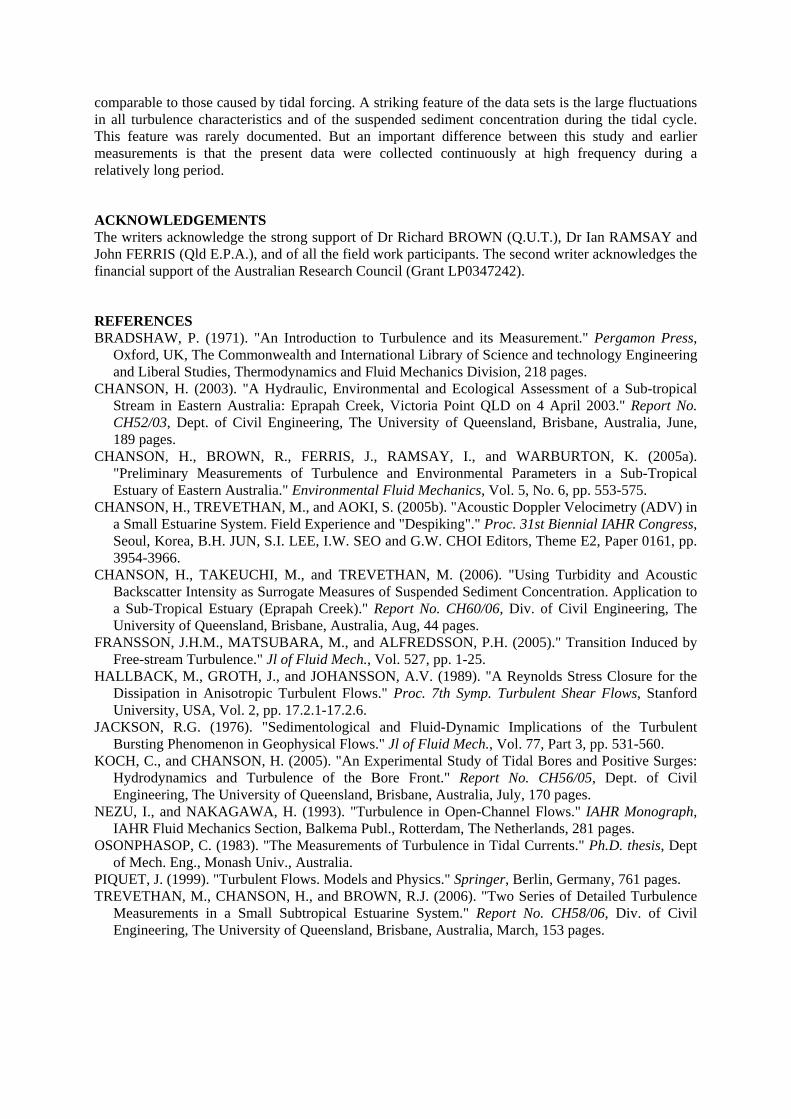
comparable to those caused by tidal forcing. A striking feature of the data sets is the large fluctuations in all turbulence characteristics and of the suspended sediment concentration during the tidal cycle. This feature was rarely documented. But an important difference between this study and earlier measurements is that the present data were collected continuously at high frequency during a relatively long period.

ACKNOWLEDGEMENTS The writers acknowledge the strong support of Dr Richard BROWN (Q.U.T.), Dr Ian RAMSAY and John FERRIS (Qld E.P.A.), and of all the field work participants. The second writer acknowledges the financial support of the Australian Research Council (Grant LP0347242).

REFERENCES BRADSHAW, P. (1971). "An Introduction to Turbulence and its Measurement." Pergamon Press,

Oxford, UK, The Commonwealth and International Library of Science and technology Engineering and Liberal Studies, Thermodynamics and Fluid Mechanics Division, 218 pages.

CHANSON, H. (2003). "A Hydraulic, Environmental and Ecological Assessment of a Sub-tropical Stream in Eastern Australia: Eprapah Creek, Victoria Point QLD on 4 April 2003." Report No. CH52/03, Dept. of Civil Engineering, The University of Queensland, Brisbane, Australia, June, 189 pages.

CHANSON, H., BROWN, R., FERRIS, J., RAMSAY, I., and WARBURTON, K. (2005a). "Preliminary Measurements of Turbulence and Environmental Parameters in a Sub-Tropical Estuary of Eastern Australia." Environmental Fluid Mechanics, Vol. 5, No. 6, pp. 553-575.

CHANSON, H., TREVETHAN, M., and AOKI, S. (2005b). "Acoustic Doppler Velocimetry (ADV) in a Small Estuarine System. Field Experience and "Despiking"." Proc. 31st Biennial IAHR Congress, Seoul, Korea, B.H. JUN, S.I. LEE, I.W. SEO and G.W. CHOI Editors, Theme E2, Paper 0161, pp. 3954-3966.

CHANSON, H., TAKEUCHI, M., and TREVETHAN, M. (2006). "Using Turbidity and Acoustic Backscatter Intensity as Surrogate Measures of Suspended Sediment Concentration. Application to a Sub-Tropical Estuary (Eprapah Creek)." Report No. CH60/06, Div. of Civil Engineering, The University of Queensland, Brisbane, Australia, Aug, 44 pages.

FRANSSON, J.H.M., MATSUBARA, M., and ALFREDSSON, P.H. (2005)." Transition Induced by Free-stream Turbulence." Jl of Fluid Mech., Vol. 527, pp. 1-25.

HALLBACK, M., GROTH, J., and JOHANSSON, A.V. (1989). "A Reynolds Stress Closure for the Dissipation in Anisotropic Turbulent Flows." Proc. 7th Symp. Turbulent Shear Flows, Stanford University, USA, Vol. 2, pp. 17.2.1-17.2.6.

JACKSON, R.G. (1976). "Sedimentological and Fluid-Dynamic Implications of the Turbulent Bursting Phenomenon in Geophysical Flows." Jl of Fluid Mech., Vol. 77, Part 3, pp. 531-560.

KOCH, C., and CHANSON, H. (2005). "An Experimental Study of Tidal Bores and Positive Surges: Hydrodynamics and Turbulence of the Bore Front." Report No. CH56/05, Dept. of Civil Engineering, The University of Queensland, Brisbane, Australia, July, 170 pages.

NEZU, I., and NAKAGAWA, H. (1993). "Turbulence in Open-Channel Flows." IAHR Monograph, IAHR Fluid Mechanics Section, Balkema Publ., Rotterdam, The Netherlands, 281 pages.

OSONPHASOP, C. (1983). "The Measurements of Turbulence in Tidal Currents." Ph.D. thesis, Dept of Mech. Eng., Monash Univ., Australia.

PIQUET, J. (1999). "Turbulent Flows. Models and Physics." Springer, Berlin, Germany, 761 pages. TREVETHAN, M., CHANSON, H., and BROWN, R.J. (2006). "Two Series of Detailed Turbulence

Measurements in a Small Subtropical Estuarine System." Report No. CH58/06, Div. of Civil Engineering, The University of Queensland, Brisbane, Australia, March, 153 pages.