High-Order Output-Based Adaptive Simulations of Turbulent ...kfid/MYPUBS/Fidkowski_Ceze_2016_SciTe… · High-Order Output-Based Adaptive Simulations of Turbulent Flow Over a Three

High-Order Output-Based Adaptive Simulations of

Turbulent Flow Over a Three Dimensionsional Bump

Krzysztof J. Fidkowski∗

Department of Aerospace Engineering, University of Michigan, Ann Arbor, MI 48109, USA

Marco A. Ceze†

NASA Ames Research Center, Moffett Field, CA, USA

This paper presents output-based high-order adaptive simulations of a three-dimensional benchmark problem for turbulence model verification. The flow over asmooth bump is modeled using the Reynolds-averaged compressible Navier-Stokesequations, with a negative-viscosity formulation of the Spalart-Allmaras (SA) one-equation closure. The initial high-order, curved, hexahedral mesh for the adaptiveruns is generated manually with sufficient boundary layer resolution to enable ro-bust convergence at the approximation orders tested. Thereafter, resolution isadded using fixed-fraction, hanging-node refinement driven by an output error in-dicator, calculated from a discrete adjoint-weighted residual. A comparison of theoutput convergence results to previous data verifies the methods used and demon-strates the benefit of high-order approximation for this case. In addition, severalimplementation details are discussed, including quality curved-mesh generation,wall distance calculation, hanging-node refinement, snapping of boundaries to thegeometry, and a nonlinear Newton continuation strategy.

I. Introduction

The Reynolds-averaged Navier-Stokes (RANS) equations remain an invaluable model routinelyused in analysis and design of aerospace vehicles. RANS simulations are computationally cheapcompared to other options for simulation turbulence because they take advantage of anisotropicmeshes that reduce the degrees of freedom required to accurately resolve thin boundary and shearlayers. However, realizing this advantage is not always straightforward, especially for high-ordermethods that use curved elements. Maintaining mesh validity in these cases, particularly in adaptivethree-dimensional simulations, remains a challenging task and a subject of ongoing research.

The combination of high-order approximation and mesh adaptation offers an attractive solutionstrategy for RANS simulations, which generally contain both smooth and singular features.1 Inaddition, output-based adaptive methods2–5 offer a systematic approach for identifying regionsof the domain that require more resolution for the prediction of scalar outputs of interest. Thesemethods also return error estimates that can improve the robustness of solution verification and theefficiency uncertainty quantification studies. It is for these reasons that we consider output-basedmethods in the present study.

In this paper, we apply a high-order adaptive solution technique to a three-dimensional bench-mark test case modeled using the RANS equations, closed with a negative-turbulent-viscosity modi-fication of the Spalart-Allmaras (SA) one-equation model.6 Many previous works have investigated

∗Associate Professor, AIAA Senior Member, [email protected]†Postdoctoral Fellow, Oak Ridge Associated Universities, [email protected]

1 of 19

American Institute of Aeronautics and Astronautics

the RANS-SA equations, including in a high-order adaptive setting.1,7–10 The majority of the latterwork has focused on demonstrating benefits of adaptive refinement and/or high-order over uniformor heuristic refinement for such flows. More recently, the authors and several other groups havecompared RANS results across discretizations and mesh types/refinement techniques, for severaltwo-dimensional benchmark problems.11 In the present work we extend the verification to threedimensions, with an in-depth study of one simulation: flow over a smooth three-dimensional bump.

The remainder of this paper is organized as follows. Section II presents the compressible Navier-Stokes equations closed with the RANS-SA model, and Section III discusses their discretizationwith a high-order discontinuous finite-element method. Section IV details several implementationaspects specific to three-dimensional RANS simulations. Section V describes the output error esti-mation and adaptation techniques, and Section VI presents results for the several benchmark casesconsidered. Section VII concludes with a summary and a discussion of possible future directions.

II. The Reynolds-Averaged Compressible Navier-Stokes Equations

The model equations in this work are compressible Navier-Stokes, Reynolds-averaged with aversion of the Spalart-Allmaras turbulence model that is modified for improved stability for negativevalues of the turbulence working variable, ν.6 The resulting Reynolds-averaged Navier-Stokes(RANS) equations are, using index notation with implied summation on repeated indices,

∂tρ + ∂j(ρuj) = 0

∂t(ρui) + ∂j(ρujui + pδij) − ∂jτij = 0

∂t(ρE) + ∂j(ρujH) − ∂j(uiτij − qj) = 0

∂t(ρν)︸︷︷︸unsteady

+ ∂j(ρuj ν)︸︷︷︸convective

− ∂j

[1

σρ(ν + νfn)∂j ν

]︸︷︷︸

diffusive

+ Sν︸︷︷︸source

= 0

(1)

where the terms have been split according to their treatment in the discretization, and where sourceterm for the ν equation is

Sν =1

σ(ν + νfn)∂jρ∂j ν −

cb2ρ

σ∂j ν∂j ν − P +D.

In the above equations, ρ is the density, ρuj is the momentum, E is the total energy, H = E + p/ρis the total enthalpy, p = (γ − 1)

(ρE − 1

2ρuiui)

is the pressure, γ is the ratio of specific heats, Pis the turbulence production, D is the turbulence destruction, and i, j index the spatial dimension,dim. The Reynolds stress, τij , is

τij = 2(µ+ µt)εij , εij =1

2(∂iuj + ∂jui)−

1

3∂kukδij .

µ is the laminar dynamic viscosity, obtained using Sutherland’s law,

µ = µref

(T

Tref

)1.5(Tref + Ts

T + Ts

), (2)

where T = p/(ρR) is the temperature, R is the gas constant for air (the difference in specific heats),and the eddy viscosity, µt, is

µt =

ρνfv1 ν ≥ 0

0 ν < 0fv1 =

χ3

χ3 + c3v1

, χ =ν

ν.

2 of 19


The heat flux, qj , is given by

qj = (κ+ κt)∂iT, κ = Cpµ/Pr, κt = Cpµt/Prt,

where Pr and Prt are the laminar and turbulent Prandtl numbers, and Cp is the specific heat atconstant pressure. The production term, P , is

P =

cb1Sρν χ ≥ 0

cb1Sρν χ < 0,

where the modified vorticity S is written as

S =

S + S S ≥ −cv2S

S +S(c2

v2S + cv3S)

(cv3 − 2cv2)S − SS < −cv2S

, S =νfv2

κ2d2, fv2 = 1− χ

1 + χfv1. (3)

In Eqn. 3, S =√

2ΩijΩij is the vorticity magnitude (summation implied on i, j), and Ωij =12(∂ivj − ∂jvi) is the vorticity tensor. d is the distance to the closest wall. The destruction term,D, is given by

D =

cw1fw

ρν2

d2χ ≥ 0

−cw1ρν2

d2χ < 0

, fw = g

(1 + c6

w3

g6 + c6w3

)1/6

, g = r + cw2(r6 − r), r =ν

Sκ2d2.

Finally, in Eqn. 1, fn = 1 for positive ν and

fn =cn1 + χ3

cn1 − χ3, when χ < 0. (4)

Relevant closure coefficients are

cb1 = 0.1355 cw1 =cb1κ2

+1 + cb2σ

cv1 = 7.1

cb2 = 0.622 cw2 = 0.3 κ = 0.41

σ = 2/3 cw3 = 2 Prt = 0.9

cn1 = 16 cv2 = 0.7 cv3 = 0.9

III. Discontinuous Galerkin Discretization

We discretize Eqn. 1 using a discontinuous Galerkin (DG) finite element method.9,12 Definingthe state vector as u = [ρ, ρui, ρE, ρν]T , we write Eqn. 1 in compact conservative form,

∂tu +∇ · ~F(u,∇u) + S(u,∇u) = 0, (5)

where ~F is the combined inviscid/viscous flux vector, and S is the source term associated with theturbulence closure equation. We approximate the state in a finite dimensional space, uh ∈ Vh,where Vh is the space of element-wise discontinuous polynomials of order p. Choosing a basis forVh yields the following state approximation on element k,

u(~x)∣∣k

=

n(p)∑j=1

Ukjφj(~x),

3 of 19


where Ukj are the six unknowns associated with basis function j on element k. We denote by U =Ukj all of these unknowns rolled into one vector. By virtue of the discontinuous approximationspace inherent to DG, the basis functions used to approximate the state need not correspond to thegeometrical shape of the element. For example, whereas tensor product basis functions are typicallyused on hexahedral elements, in DG one can also use full-order “tetrahedral” basis functions. Thisresults in a significant savings in degrees of freedom for the same nominal order of convergence: forexample, a p = 4 tensor product basis requires 125 unknowns per element, while a p = 4 full-orderbasis only requires 35 unknowns per element. This yields storage savings factors of over 3.5 for thestate and 12 for the residual Jacobian matrix.

Multiplying Eqn. 5 by test functions in Vh, which are the same as the basis functions for DG,integrating by parts on each element, and using the Roe13 convective flux and the second form ofBassi and Rebay (BR2)14 for the viscous treatment, we obtain the following system of nonlinearequations,

R(U) = 0. (6)

III.A. Symmetry boundary conditions

The bump case presently considered requires symmetry boundary conditions on several boundaries.In the continuous limit, symmetry requires vanishing normal state derivatives. A finite-dimensionalsolution will generally violate these requirements pointwise, so we must enforce the BC weakly. Thisenforcement involves transforming the state and gradient, similarly to methods in previous works,15

though we construct a state/gradient on the boundary instead of employing a ghost cell. Startingwith the state, we require that at a symmetry boundary all vectors in the state (e.g. a velocity) havetheir normal components zeroed out. This results in a linear transformation from the interior (u+)to the boundary (ub) state vector, which reads ub = Au+. A is the identity matrix for all statesexcept the momentum, which transforms as (ρ~v)b = V (ρ~v)+, where V = I − ~n⊗ ~n = δij − ninj . ~nis the outward-pointing normal, and I = δij is the dim×dim identity matrix.

The state gradient transformation must account for possibly nonzero normal velocity com-ponents. We first consider a hypothetical ghost state (u−) and gradient (∇u−), obtained byreflecting the velocity about the symmetry plane. Specifically, u− = Bu+, where B is an iden-tity matrix for all states except the momentum, which transforms as (ρ~v)− = W (ρ~v)+, whereW = I − 2~n ⊗ ~n = δij − 2ninj . Note that B = 2A − I and that W = 2V − I. Differentiatingthe expression for u− in space gives the gradient, which we must reflect by applying W , so that∇u− = B∇u+W T . Finally, we obtain the gradient at the boundary, ∇ub, by averaging the interiorand exterior gradients – this is consistent with what would happen in the viscous flux calculationif there were actually a symmetrical mesh on the other side of the symmetry line. So we have

∇ub =1

2

(∇u+ +∇u−

)=

1

2

(∇u+ + B∇u+W T

)=

1

2

(∇u+ + (2A− I)∇u+(2V T − I)

)= ∇u+ + A∇u+(2V T − I)−∇u+V = ∇u+~n⊗ ~n+ A∇u+(I − 2~n⊗ ~n).

III.B. Scaling of ν

The SA working variable, ν, will generally be orders of magnitude smaller than the other statecomponents. We use scaling or “non-dimensionalization” of ν to make its range of numerical valuessimilar to the other state components. This proves to be effective in improving the performance ofthe linear and nonlinear solvers.12 We store the scaled quantity, ρν ′, given by

ρν ′ =ρν

κSAµ∞,

4 of 19


where κSA is a scaling factor, typically O(√Re), and µ∞ is the free-stream laminar dynamic

viscosity. In addition, the SA ν equation is divided by κSAµ∞.

IV. Implementation

IV.A. Mesh Generation

A curved, hexahedral mesh was generated manually as a starting mesh for the adaptive runs. High-order curved elements provide geometric fidelity that is essential for robust and accurate solutionsvia the discontinuous Galerkin method, even at solution approximation orders of p = 1.16 In thiswork, we employ curved elements throughout the domain, as the presence of highly-anisotropicelements near the wall precludes the use of just one layer of curved elements. The anisotropyis motivated by efficiency: RANS simulations require much higher resolution, i.e. smaller lengthscales, perpendicular to the wall compared to parallel to the wall, so that anisotropic “pancake”elements reduce the total degrees of freedom without sacrificing accuracy.

In this work, each hexahedron in physical space is obtained by mapping a unit reference cubevia tensor-product polynomials of order q, as shown in Figure 1. Nodal Lagrange basis functions,with equal node spacing in reference space, yield curved elements that interpolate the providednodes, (q + 1)3 total. This property is useful for defining curved hexahedra via the coordinates oftheir (q + 1)3 nodes.

X

Y

Z

y

x

z

reference space global space

~x =∑n(q)

j=1 ~xjφj(~X)

Figure 1. Reference-to-global mapping for a hexahedral elements, shown for q = 2 geometry approximationwith 27 nodes.

The high-order nodes inside the elements should be spaced roughly uniformly in physical space,unless attempting to optimize the elements’ approximation power,17 to minimize skewness andavoid the risk of negative mapping Jacobians. However, the elements themselves should ideallybe distributed non-uniformly over the domain to provide efficient solution approximation. In thiswork we use logarithmic spacing for the element corner nodes, and linear spacing for the in-betweenhigh-order nodes, as illustrated in Figure 2. For the present bump problem, these spacings areprescribed for a uniform lattice in a featureless duct, which is then deformed and blended to fit thegiven geometry.

Several remarks about the high-order meshes are in order. First, the meshes are watertight byvirtue of the uniqueness of edge and face approximations. That is, each edge is fully defined by thenodes on that edge, regardless of the positions of the other nodes in the element. The same is truefor the faces. Second, although we use high-order curved elements, slope/normal continuity is notexplicitly enforced at inter-element boundaries. However, the mismatch in the slope, along withthe geometry errors in general, diminish as the mesh is refined. Third, curved elements requirenon-canonical mass matrices, and these are computed via quadrature and stored for the duration ofthe run. Finally, when a mesh is adapted, new nodes placed on the curved boundary are snapped tothe geometry. This demands sufficient resolution from the initial mesh to prevent element inversion,

5 of 19


Figure 2. To increase resolution near the bump wall, elements (the boundaries of which are denoted by blacklines) are spaced logarithmically away from the wall. However, to minimize element skewness, the nodes insideeach element (identified by the blue triangulation) are spaced uniformly.

as only the first layer of elements adjacent to the boundary is affected by the snapping.

IV.B. Wall Distance Calculation

The distance to the closest wall, d, is required for the Spalart-Allmaras turbulence model. Thisdistance is used at every quadrature point, during the construction of the residual and resid-ual Jacobian matrix. Rather than separately storing the distance at every quadrature point, thewall distance is approximated by a polynomial of order pwd on each element. This polynomial isconstructed by evaluating the wall distance at each Lagrange node used in the polynomial approx-imation on an element.

The wall distance is calculated at each order pwd Lagrange node of each element using thefollowing procedure. First, the distance to each boundary node is calculated via a brute-forceprocedure to pre-select the closest boundary faces, which are those adjacent to the closest node.For each of these boundary faces, which can generally be curved, the wall distance is computedby first subdividing the high-order face into linear triangles, with 2(q + 1) subdivisions along eachedge. Thus, a quadrilateral boundary face would be split into 2[2(q+1)]2 = 8(q+1)2 triangles. Thedistance to each of these triangles is computed by projection, and the closest triangle is selected.The minimum distance to the linear triangles could be used as an estimate of the wall distance,though it could be insufficiently accurate for highly-curved faces. Rather, the projection of the pointin question onto the closest triangle defines reference-space coordinates on the original face thatare used to “snap” the projection to the curved face geometry via the reference-to-global geometrymapping, as illustrated in Figure 3. The distance to this snapped projection then defines the walldistance. For further accuracy, the projection could serve as an initial guess for Newton-Raphsoniterations to minimize the distance on the curved face, though this extra step has not been foundto produce additional accuracy gains above the geometry approximation error of the curved faces,as indicated by the wall distance error study in Figure 4.

6 of 19


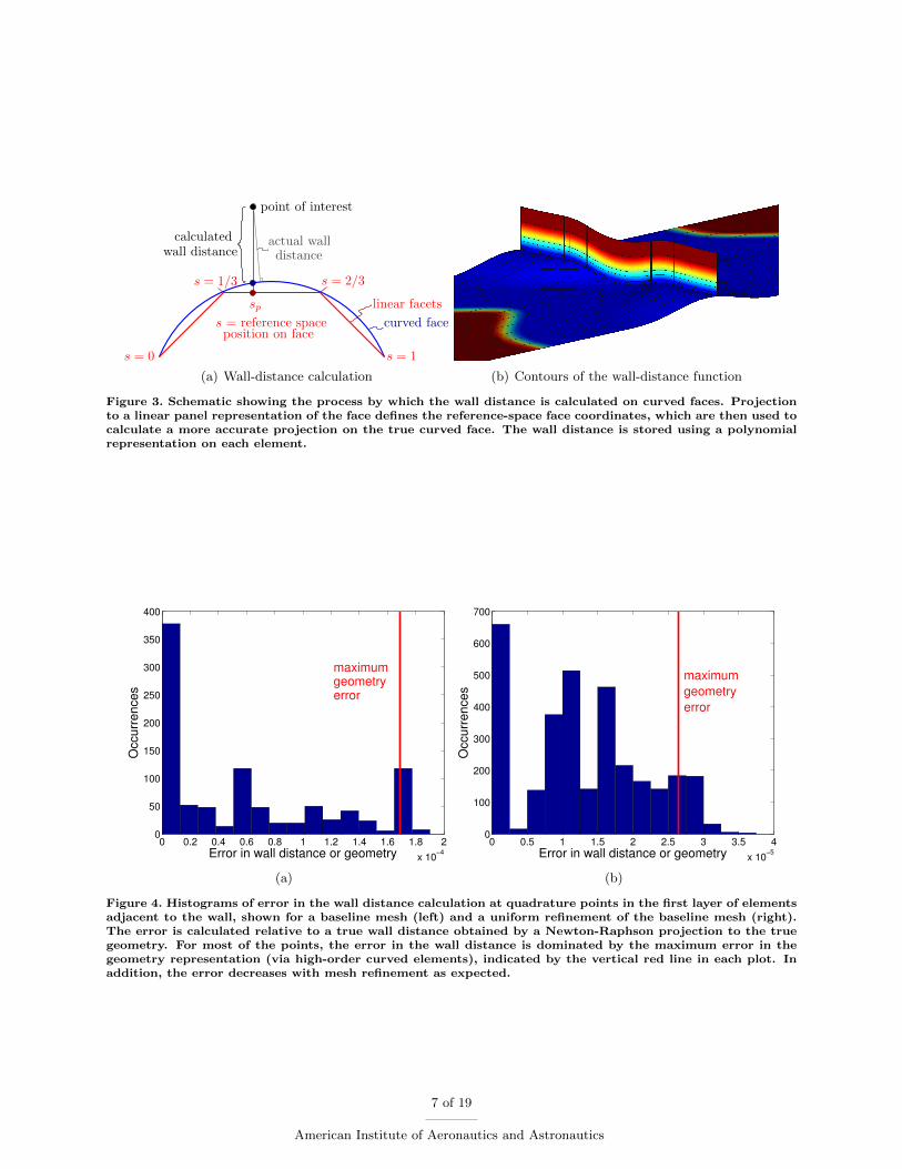
actual wallcalculatedwall distance distance

point of interest

sp

s = 2/3

s = 1s = 0

s = 1/3

position on faces = reference space

linear facets

curved face

(a) Wall-distance calculation (b) Contours of the wall-distance function

Figure 3. Schematic showing the process by which the wall distance is calculated on curved faces. Projectionto a linear panel representation of the face defines the reference-space face coordinates, which are then used tocalculate a more accurate projection on the true curved face. The wall distance is stored using a polynomialrepresentation on each element.

0 0.2 0.4 0.6 0.8 1 1.2 1.4 1.6 1.8 2

x 10−4

0

50

100

150

200

250

300

350

400

Error in wall distance or geometry

Occurr

ences

maximumgeometryerror

(a)

0 0.5 1 1.5 2 2.5 3 3.5 4

x 10−5

0

100

200

300

400

500

600

700

Error in wall distance or geometry

Occurr

ences

maximum

geometry

error

(b)

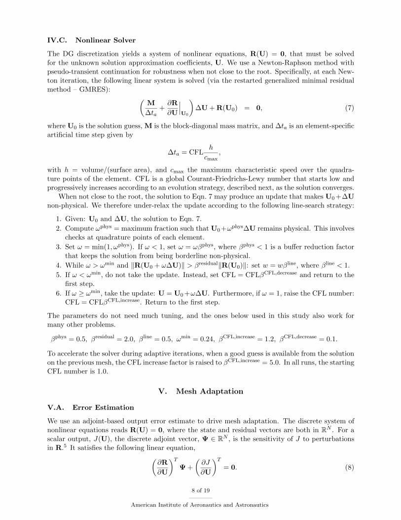
Figure 4. Histograms of error in the wall distance calculation at quadrature points in the first layer of elementsadjacent to the wall, shown for a baseline mesh (left) and a uniform refinement of the baseline mesh (right).The error is calculated relative to a true wall distance obtained by a Newton-Raphson projection to the truegeometry. For most of the points, the error in the wall distance is dominated by the maximum error in thegeometry representation (via high-order curved elements), indicated by the vertical red line in each plot. Inaddition, the error decreases with mesh refinement as expected.

7 of 19


IV.C. Nonlinear Solver

The DG discretization yields a system of nonlinear equations, R(U) = 0, that must be solvedfor the unknown solution approximation coefficients, U. We use a Newton-Raphson method withpseudo-transient continuation for robustness when not close to the root. Specifically, at each New-ton iteration, the following linear system is solved (via the restarted generalized minimal residualmethod – GMRES): (

M

∆ta+∂R

∂U

∣∣∣U0

)∆U + R(U0) = 0, (7)

where U0 is the solution guess, M is the block-diagonal mass matrix, and ∆ta is an element-specificartificial time step given by

∆ta = CFLh

cmax,

with h = volume/(surface area), and cmax the maximum characteristic speed over the quadra-ture points of the element. CFL is a global Courant-Friedrichs-Lewy number that starts low andprogressively increases according to an evolution strategy, described next, as the solution converges.

When not close to the root, the solution to Eqn. 7 may produce an update that makes U0 +∆Unon-physical. We therefore under-relax the update according to the following line-search strategy:

1. Given: U0 and ∆U, the solution to Eqn. 7.

2. Compute ωphys = maximum fraction such that U0 +ωphys∆U remains physical. This involveschecks at quadrature points of each element.

3. Set ω = min(1, ωphys). If ω < 1, set ω = ωβphys, where βphys < 1 is a buffer reduction factorthat keeps the solution from being borderline non-physical.

4. While ω > ωmin and ‖R(U0 + ω∆U)‖ > βresidual‖R(U0)‖: set w = wβline, where βline < 1.

5. If ω < ωmin, do not take the update. Instead, set CFL = CFLβCFL,decrease and return to thefirst step.

6. If ω ≥ ωmin, take the update: U = U0 +ω∆U. Furthermore, if ω = 1, raise the CFL number:CFL = CFLβCFL,increase. Return to the first step.

The parameters do not need much tuning, and the ones below used in this study also work formany other problems.

βphys = 0.5, βresidual = 2.0, βline = 0.5, ωmin = 0.24, βCFL,increase = 1.2, βCFL,decrease = 0.1.

To accelerate the solver during adaptive iterations, when a good guess is available from the solutionon the previous mesh, the CFL increase factor is raised to βCFL,increase = 5.0. In all runs, the startingCFL number is 1.0.

V. Mesh Adaptation

V.A. Error Estimation

We use an adjoint-based output error estimate to drive mesh adaptation. The discrete system ofnonlinear equations reads R(U) = 0, where the state and residual vectors are both in RN . For ascalar output, J(U), the discrete adjoint vector, Ψ ∈ RN , is the sensitivity of J to perturbationsin R.5 It satisfies the following linear equation,(

∂R

∂U

)TΨ +

(∂J

∂U

)T= 0. (8)

8 of 19


The adjoint vector provides an estimate of the error in the output when computing on a finite-dimensional approximation space. Consider two finite-dimensional spaces: a coarse approximationspace, VH , on which we calculate the state and output, and a fine space, Vh (obtained by incre-menting the approximation order by 1), on which we compute the adjoint and relative to which weestimate the error. We would like to measure the output error in the coarse solution relative to thefine space,

output error: δJ ≡ JH(UH)− Jh(Uh). (9)

We assume that the fine approximation space contains the coarse approximation space, so that alossless state injection, UH

h ≡ IHh UH , exists, where IHh is the coarse-to-fine state injection (prolon-gation) operator. The fine-space solution, Uh ∈ RNh , solves Rh(Uh) = 0, but the injected statewill generally not give zero fine-space residuals, Rh(UH

h ) 6= 0. Instead, the injected coarse statesolves a perturbed fine-space problem, Rh(U′h) − Rh(UH

h ) = 0, and the fine-space adjoint, Ψh,tells us to expect an output perturbation given by the inner product between the adjoint and theresidual perturbation,

δJ ≈ −ΨThRh(UH

h ). (10)

This estimate assumes small perturbations in the state when the output or equations are nonlinear.It does not require the fine-space primal solution, Uh, but it does require the fine-space adjoint. Inthis work, we fully converge the fine-space adjoint about the injected state, UH

h , storing the fine-space Jacobian and using ΨH

h ≡ IHh ΨH as a initial guess in the GMRES iterative solver for Ψh.For the three-dimensional problem considered in this work, this does add non-trivial additionalcomputational cost and memory overhead. However, we do this to minimize additional sourcesof error. In practice, techniques such as iterative smoothing or reconstruction can be used toapproximate the fine-space adjoint and reduce the cost.5,9, 12

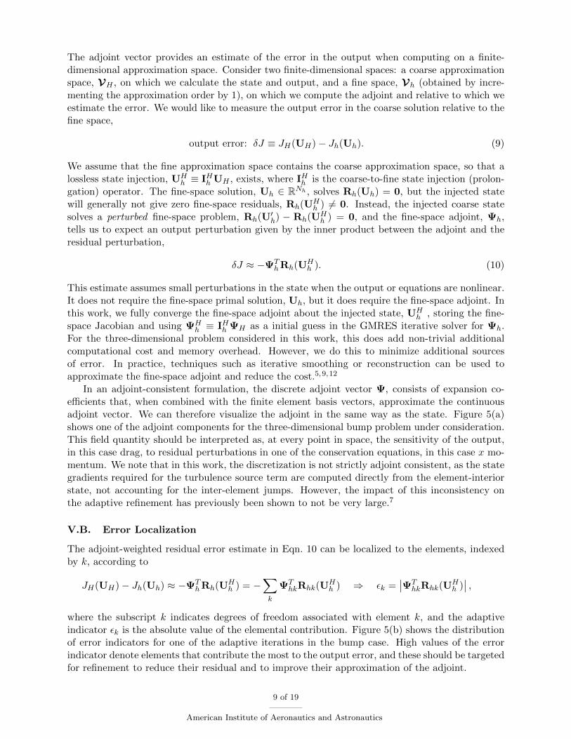
In an adjoint-consistent formulation, the discrete adjoint vector Ψ, consists of expansion co-efficients that, when combined with the finite element basis vectors, approximate the continuousadjoint vector. We can therefore visualize the adjoint in the same way as the state. Figure 5(a)shows one of the adjoint components for the three-dimensional bump problem under consideration.This field quantity should be interpreted as, at every point in space, the sensitivity of the output,in this case drag, to residual perturbations in one of the conservation equations, in this case x mo-mentum. We note that in this work, the discretization is not strictly adjoint consistent, as the stategradients required for the turbulence source term are computed directly from the element-interiorstate, not accounting for the inter-element jumps. However, the impact of this inconsistency onthe adaptive refinement has previously been shown to not be very large.7

V.B. Error Localization

The adjoint-weighted residual error estimate in Eqn. 10 can be localized to the elements, indexedby k, according to

JH(UH)− Jh(Uh) ≈ −ΨThRh(UH

h ) = −∑k

ΨThkRhk(U

Hh ) ⇒ εk =

∣∣ΨThkRhk(U

Hh )∣∣ ,

where the subscript k indicates degrees of freedom associated with element k, and the adaptiveindicator εk is the absolute value of the elemental contribution. Figure 5(b) shows the distributionof error indicators for one of the adaptive iterations in the bump case. High values of the errorindicator denote elements that contribute the most to the output error, and these should be targetedfor refinement to reduce their residual and to improve their approximation of the adjoint.

9 of 19


(a) Drag adjoint (b) Adaptive indicator

Figure 5. Flow over a three-dimensional bump: the conservation of x-momentum component of the drag adjointon a medium resolution mesh, and the localized output error which serves as the adaptive indicator.

V.C. Hanging-Node Hexahedral Mesh Refinement

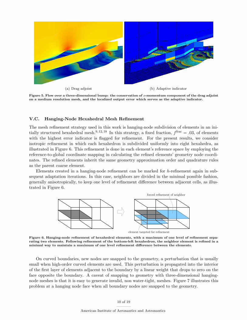
The mesh refinement strategy used in this work is hanging-node subdivision of elements in an ini-tially structured hexahedral mesh.9,12,18 In this strategy, a fixed fraction, f frac = .03, of elementswith the highest error indicator is flagged for refinement. For the present results, we considerisotropic refinement in which each hexahedron is subdivided uniformly into eight hexahedra, asillustrated in Figure 6. This refinement is done in each element’s reference space by employing thereference-to-global coordinate mapping in calculating the refined elements’ geometry node coordi-nates. The refined elements inherit the same geometry approximation order and quadrature rulesas the parent coarse element.

Elements created in a hanging-node refinement can be marked for h-refinement again in sub-sequent adaptation iterations. In this case, neighbors are divided in the minimal possible fashion,generally anisotropically, to keep one level of refinement difference between adjacent cells, as illus-trated in Figure 6.

element targeted for refinement

forced refinement of neighbor

Figure 6. Hanging-node refinement of hexahedral elements, with a maximum of one level of refinement sepa-rating two elements. Following refinement of the bottom-left hexahedron, the neighbor element is refined in aminimal way to maintain a maximum of one level refinement difference between the elements.

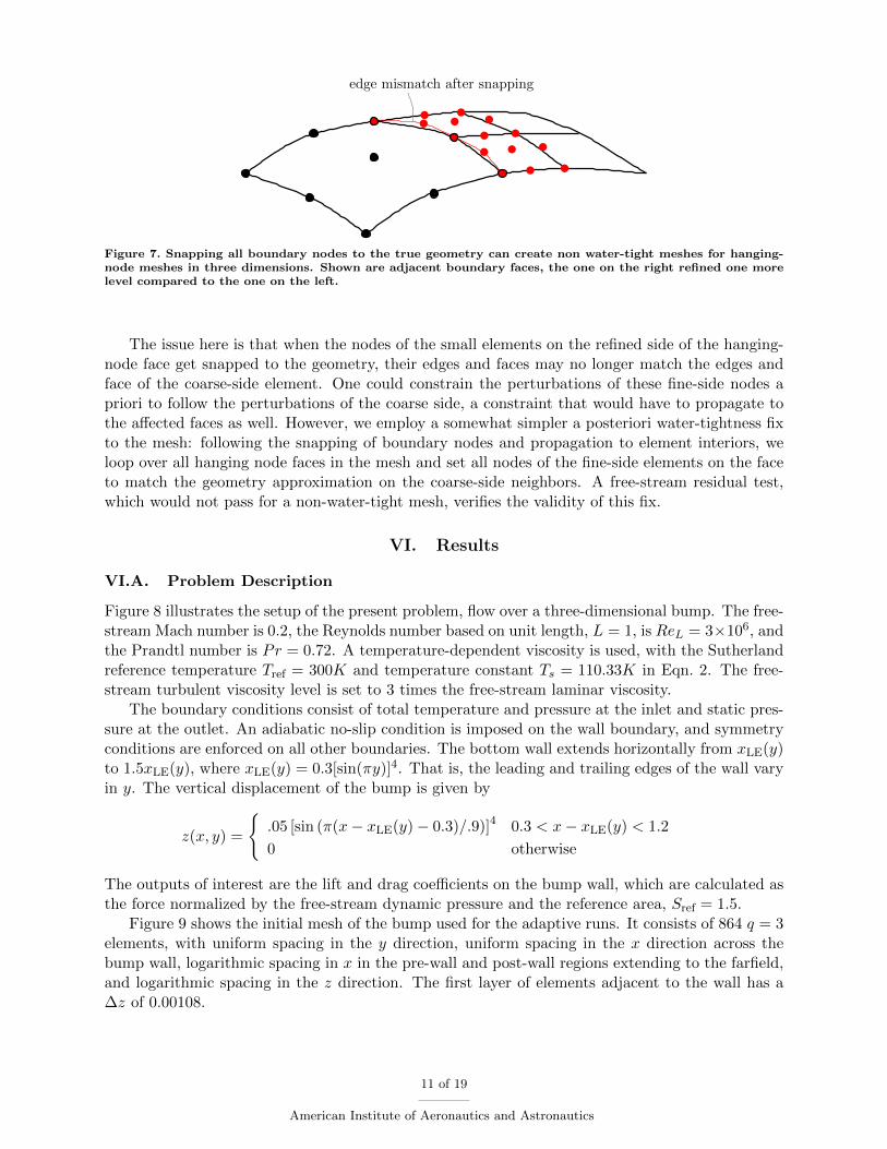
On curved boundaries, new nodes are snapped to the geometry, a perturbation that is usuallysmall when high-order curved elements are used. This perturbation is propagated into the interiorof the first layer of elements adjacent to the boundary by a linear weight that drops to zero on theface opposite the boundary. A caveat of snapping to geometry with three-dimensional hanging-node meshes is that it is easy to generate invalid, non water-tight, meshes. Figure 7 illustrates thisproblem at a hanging node face when all boundary nodes are snapped to the geometry.

10 of 19


edge mismatch after snapping

Figure 7. Snapping all boundary nodes to the true geometry can create non water-tight meshes for hanging-node meshes in three dimensions. Shown are adjacent boundary faces, the one on the right refined one morelevel compared to the one on the left.

The issue here is that when the nodes of the small elements on the refined side of the hanging-node face get snapped to the geometry, their edges and faces may no longer match the edges andface of the coarse-side element. One could constrain the perturbations of these fine-side nodes apriori to follow the perturbations of the coarse side, a constraint that would have to propagate tothe affected faces as well. However, we employ a somewhat simpler a posteriori water-tightness fixto the mesh: following the snapping of boundary nodes and propagation to element interiors, weloop over all hanging node faces in the mesh and set all nodes of the fine-side elements on the faceto match the geometry approximation on the coarse-side neighbors. A free-stream residual test,which would not pass for a non-water-tight mesh, verifies the validity of this fix.

VI. Results

VI.A. Problem Description

Figure 8 illustrates the setup of the present problem, flow over a three-dimensional bump. The free-stream Mach number is 0.2, the Reynolds number based on unit length, L = 1, is ReL = 3×106, andthe Prandtl number is Pr = 0.72. A temperature-dependent viscosity is used, with the Sutherlandreference temperature Tref = 300K and temperature constant Ts = 110.33K in Eqn. 2. The free-stream turbulent viscosity level is set to 3 times the free-stream laminar viscosity.

The boundary conditions consist of total temperature and pressure at the inlet and static pres-sure at the outlet. An adiabatic no-slip condition is imposed on the wall boundary, and symmetryconditions are enforced on all other boundaries. The bottom wall extends horizontally from xLE(y)to 1.5xLE(y), where xLE(y) = 0.3[sin(πy)]4. That is, the leading and trailing edges of the wall varyin y. The vertical displacement of the bump is given by

z(x, y) =

.05 [sin (π(x− xLE(y)− 0.3)/.9)]4 0.3 < x− xLE(y) < 1.2

0 otherwise

The outputs of interest are the lift and drag coefficients on the bump wall, which are calculated asthe force normalized by the free-stream dynamic pressure and the reference area, Sref = 1.5.

Figure 9 shows the initial mesh of the bump used for the adaptive runs. It consists of 864 q = 3elements, with uniform spacing in the y direction, uniform spacing in the x direction across thebump wall, logarithmic spacing in x in the pre-wall and post-wall regions extending to the farfield,and logarithmic spacing in the z direction. The first layer of elements adjacent to the wall has a∆z of 0.00108.

11 of 19


xLE(y)

1.5 + xLE(y)

y = 0

y = −1y

z

x

z = 5

inflow at x = −25

outflow at x = 26.5

z(x, y): wall

Figure 8. Setup for the bump problem.

(a) Zoomed-out view (b) Zoomed-in view

Figure 9. Initial mesh used for the adaptive simulations, consisting of 864 q = 3 elements.

12 of 19


VI.B. Output Convergence

Starting from the initial mesh, solutions at prescribed orders, p, were converged using the nonlinearsolver outlined in Section IV.C with βCFL,increase = 1.2. A full-order “tetrahedral” basis was usedto reduce the size of the systems at high orders compared to the tensor-product “hexahedral”basis. Order continuation was used, where the solution at order p was used to initialize the stateat order p + 1. Free-stream initial conditions were used for p = 1. Following convergence on theinitial mesh, adaptive refinements were performed at each order p using the hanging node strategydescribed in Section V.C with f frac = .03. Both lift and drag output adjoints were used to driveseparate refinement sequences. Since the solution was not expected to change much between theadaptive iterations, a more aggressive CFL increase factor of βCFL,increase = 5 was used to speedup convergence.

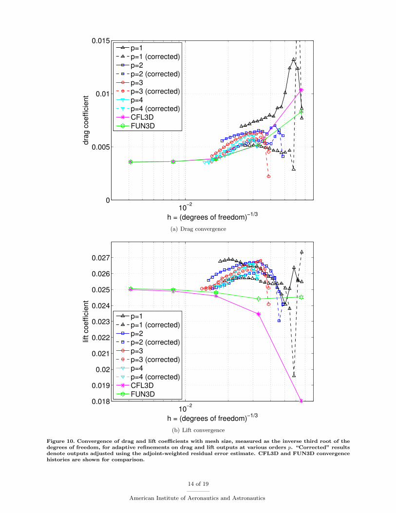
Figure 10 shows the convergence of the drag and lift coefficients with adaptive refinement. Thedata are shown as output versus h, which is a measure of the mesh size defined as h = (dof)−1/3. Fora mesh with isotropic elements, all of the same size, this would correspond to the mesh diameter.For our adapted and anisotropic meshes, this is no longer the case, and instead h is a surrogatemeasure of the number of degrees of freedom: the larger the h the fewer the degrees of freedom,the cheaper the cost. In addition to the raw output data at each order p, Figure 10 also showsthe “corrected” outputs, which are obtained by subtracting the adjoint-weighted residual outputerror estimate, δJ in Eqn. 10, from the computed output. In the asymptotic regime and when theadjoint is solved to sufficient accuracy, this correction should yield a faster converging output.

As shown in Figure 10 the DG results in this work appear to eventually, for fine meshes andhigh orders, converge to the same results obtained using the CFL3D and FUN3D codes, the datafor which was provided on the NASA turbulence modeling resource website. At order p = 1,the convergence is not yet apparent and from the trend would require many more iterations (amuch smaller h) to converge. The corrected p = 1 result is closer to the expected true value,but its convergence is also not very rapid. Order p = 2 performs better, with a more rapidconvergence, especially for the lift output at the finer meshes. In addition, the corrected p = 2result appears competitive with the CFL3D and FUN3D data at similar degrees of freedom. As theorder increases, the convergence improves further, with the p = 4 raw and corrected data showingvery good convergence to the results predicted by the fine CFL3D and FUN3D runs.

VI.C. Adapted Meshes

The adaptive refinement strategy selectively increases resolution in areas where nonzero residualsare present and affect the output of interest the most. The resulting adapted meshes are specific tothe output calculated and to the order of approximation used. We take a close look at the meshesobtained at the 10th adaptive iteration, for the drag and lift outputs, using approximation ordersp = 1 an p = 4.

Figures 11 and 12 show the meshes adapted to the drag and lift outputs respectively, at p = 1approximation order. We see similar, though not identical, refinement patterns. Both outputs aresensitive to the leading-edge region and to the crest of the bump. The regions before and after thebump are refined in slightly different fashions: the drag-adapted mesh shows increased resolutionin these regions, especially near the wall at the x = 1.2 cut.

Figures 13 and 14 show the drag- and lift-adapted meshes for order p = 4. These are also atthe 10th adaptive iteration, and given the same adaptive refinement fraction, they have a numberof elements similar to the p = 1 meshes. However, the distribution of resolution at p = 4 differsmarkedly from that at p = 1. We see much less resolution added away from the wall at the higherorder, indicating that this region is relatively well-resolved compared to the region near the wall,where the density of elements is high for p = 4. This translates into more surface refinement and

13 of 19


10−2

0

0.005

0.01

0.015

h = (degrees of freedom)−1/3

dra

g c

oe

ffic

ien

t

p=1p=1 (corrected)p=2p=2 (corrected)p=3p=3 (corrected)p=4p=4 (corrected)CFL3DFUN3D

(a) Drag convergence

10−2

0.018

0.019

0.02

0.021

0.022

0.023

0.024

0.025

0.026

0.027

h = (degrees of freedom)−1/3

lift

co

eff

icie

nt

p=1p=1 (corrected)p=2p=2 (corrected)p=3p=3 (corrected)p=4p=4 (corrected)CFL3DFUN3D

(b) Lift convergence

Figure 10. Convergence of drag and lift coefficients with mesh size, measured as the inverse third root of thedegrees of freedom, for adaptive refinements on drag and lift outputs at various orders p. “Corrected” resultsdenote outputs adjusted using the adjoint-weighted residual error estimate. CFL3D and FUN3D convergencehistories are shown for comparison.

14 of 19


(a) 3D view (b) Cuts at x = 0.3 (top), x = 0.75, and x = 1.2

Figure 11. Mesh at the 10th drag-based adaptive iteration (6213 elements) using p = 1 approximation.


Figure 12. Mesh at the 10th lift-based adaptive iteration (6357 elements) using p = 1 approximation.

15 of 19


more refinement of the boundary layer just off the wall at p = 4. Also, comparing the drag- andlift-adapted meshes, we see that the drag output requires more resolution on the bump crest andaft of the bump, whereas the lift output requires more resolution at the leading-edge region andin regions further away from the wall. The refinement patterns are relatively smooth, suggestingthat the effect of the adjoint inconsistency in the turbulent source term treatment on the meshrefinement is not strong.


Figure 13. Mesh at the 10th drag-based adaptive iteration (6280 elements) using p = 4 approximation.


Figure 14. Mesh at the 10th lift-based adaptive iteration (6627 elements) using p = 4 approximation.

VI.D. Field Plots

Figure 15 shows a selection of field quantities for a relatively well-resolved mesh, using p = 4approximation order. The pressure contours are smooth and show the expected trend of lowpressure over the crest of the bump and pressure buildup near the leading-edge regions. Theturbulent viscosity contours at various x locations show an increasingly thicker turbulent viscositylayer, with three-dimensional structure – a strong core in the center at x = 2.4 downstream of thebump wall. The Mach number contours show the expected no-slip boundary condition at the bump

16 of 19


wall, and a thin boundary layer region that increases in thickness aft of the bump. Finally, theentropy contours show generation of entropy over the surface of the wall, with larger levels on thebump crest.

(a) Pressure coefficient, cp (-0.64 to 0.22) (b) ν at x = 0.3(top), 1.2, 2.4; (0 to 60/240/750ν∞)

(c) Mach contours (0 to 0.25) (d) Entropy contours

Figure 15. Plots of several field quantities on a fine mesh, using p = 4 approximation order.

VII. Conclusions

This paper has presented the results of adaptive simulations for Reynolds-averaged turbulentflow over a three-dimensional bump, using a high-order discontinuous Galerkin finite element dis-cretization. Details on the fluid model and the discretization were presented, notably regardinggeneration of curved meshes, calculation of the wall distance, and solution of the nonlinear systemvia pseudo-time stepping. Adaptive refinement was driven by an adjoint-weighted residual, withthe output-specific discrete adjoint solution computed on a finer space providing residual sensitivityinformation. Hanging-node adaptation was employed to increase resolution, with a water-tightnessenforcement to ensure mesh validity when snapping boundary points to the true geometry. Thethree-dimensional runs were performed on hexahedral elements but using a tetrahedral, full-order,basis in order to significantly reduce the size of the system for the same formal convergence order.

The adaptive results show that when using high-order approximation, both the drag and liftoutputs converge to the asymptotic values predicted by previous CFL3D and FUN3D runs. De-

17 of 19


pending on the accuracy tolerance, there is an advantage of the high-order DG simulations of upto an order of magnitude in degrees of freedom (slightly more than a factor of two in h) over theCFL3D and FUN3D runs. However, this advantage does not directly extend to computational time,as degrees of freedom in high-order DG simulations are generally more computationally expensivethan those for second-order finite volume simulations. We also note that the incorporation of theoutput error estimate improves the convergence of the output, but that there is still a large pre-asymptotic region in which the output is far away from the truth value and the correction, basedon linearized theory, does not uncover all of the error. This effect is strongest at the lower orders,suggesting another reason for using high-order approximation.

Further benefits in adaptive three-dimensional simulations will likely be achieved by more gen-eral adaptive mechanics, e.g. using fully-unstructured tetrahedral meshes, or hybrid prismatic andtetrahedral meshes, for which the impact of the initial mesh quality is not as limiting. In addi-tion, even for hanging-node refinement, anisotropic h refinement and combined h and p refinementshould provide noticeable improvements compared to the isotropic h strategy employed in thiswork. Nevertheless, this study verified both the fluid model and the ability of adjoint-based refine-ment to successfully target the desired output with incremental resolution in small portions of thethree-dimensional domain.

References

1Yano, M., Modisette, J., and Darmofal, D., “The importance of mesh adaptation for higher-order discretizationsof aerodynamics flows,” AIAA Paper 2011-3852, 2011.

2Becker, R. and Rannacher, R., “An optimal control approach to a posteriori error estimation in finite elementmethods,” Acta Numerica, edited by A. Iserles, Cambridge University Press, 2001, pp. 1–102.

3Venditti, D. A. and Darmofal, D. L., “Anisotropic grid adaptation for functional outputs: application totwo-dimensional viscous flows,” Journal of Computational Physics, Vol. 187, No. 1, 2003, pp. 22–46.

4Hartmann, R. and Houston, P., “Adaptive discontinuous Galerkin finite element methods for the compressibleEuler equations,” Journal of Computational Physics, Vol. 183, No. 2, 2002, pp. 508–532.

5Fidkowski, K. J. and Darmofal, D. L., “Review of output-based error estimation and mesh adaptation incomputational fluid dynamics,” American Institute of Aeronautics and Astronautics Journal , Vol. 49, No. 4, 2011,pp. 673–694.

6Allmaras, S., Johnson, F., and Spalart, P., “Modifications and clarifications for the implementation of theSpalart-Allmaras turbulence model,” Seventh International Conference on Computational Fluid Dynamics (ICCFD7)1902, 2012.

7Oliver, T. A., A High–order, Adaptive, Discontinuous Galerkin Finite Elemenet Method for the Reynolds-Averaged Navier-Stokes Equations, Ph.D. thesis, Massachusetts Institute of Technology, Cambridge, Massachusetts,2008.

8Oliver, T. A. and Darmofal, D. L., “Impact of turbulence model irregularity on high–order discretizations,”AIAA Paper 2009-953, 2009.

9Ceze, M. A. and Fidkowski, K. J., “An anisotropic hp-adaptation framework for functional prediction,” Amer-ican Institute of Aeronautics and Astronautics Journal , Vol. 51, 2013, pp. 492–509.

10Yano, M., An Optimization Framework for Adaptive Higher-Order Discretizations of Partial Differential Equa-tions on Anisotropic Simplex Meshes, Ph.D. thesis, Massachusetts Institute of Technology, Cambridge, Massachusetts,2012.

11Ceze, M. A. and Fidkowski, K. J., “High-order output-based adaptive simulations of turbulent flow in twodimensions,” AIAA Paper 2015–1532, 2015.

12Ceze, M. A. and Fidkowski, K. J., “Drag prediction using adaptive discontinuous finite elements,” AIAAJournal of Aircraft , Vol. 51, No. 4, 2014, pp. 1284–1294.

13Roe, P. L., “Approximate Riemann solvers, parameter vectors, and difference schemes,” Journal of Computa-tional Physics, Vol. 43, 1981, pp. 357–372.

14Bassi, F. and Rebay, S., “Numerical evaluation of two discontinuous Galerkin methods for the compressibleNavier-Stokes equations,” International Journal for Numerical Methods in Fluids, Vol. 40, 2002, pp. 197–207.

15Leicht, T. and Hartmann, R., “Error estimation and anisotropic mesh refinement for 3D laminar aerodynamicflow simulations,” Journal of Computational Physics, Vol. 229, 2010, pp. 7344–7360.

18 of 19


16Bassi, F. and Rebay, S., “High–order accurate discontinuous finite element solution of the 2-D Euler equations,”Journal of Computational Physics, Vol. 138, 1997, pp. 251–285.

17Sanjaya, D. P. and Fidkowski, K. J., “Improving high-order finite element approximation through geometricalwarping,” AIAA Paper 2015–2605, 2015.

18Ceze, M. A. and Fidkowski, K. J., “Output-driven anisotropic mesh adaptation for viscous flows using discretechoice optimization,” AIAA Paper 2010-0170, 2010.

19 of 19


Documents

High-Order Output-Based Adaptive Simulations of Turbulent ...kfid/MYPUBS/Fidkowski_Ceze_2016_SciTe… · High-Order Output-Based Adaptive Simulations of Turbulent Flow Over a Three