HIGH POWER OPERATION OF TWO SIDE-COUPLEDSTANDING WAVE LINAC STRUCTURES

by

J. McKeown, H.R. Schneider and s.o. SchriberAtomic Energy of Canada LimitedChalk River Nuclear Laboratories

Chalk River, Ontario, Canada

Introduction

The 805 MHz side coupler linearaccelerator design developed at Los Alamosand operated successfully there at six percent duty factor, has been tested to higheraverage powers at Chalk River NuclearLaboratories. Two side coupled cavity tankshave been built and operated at power levelsin excess of 50 kW at 100% duty factor. Oneof the tanks (Modell) was built solely forinvestigating high power operation, whilethe other (Model 4) is a pre-acceleratorsection of a 4 MeV high intensity electronlinac (1).

Tank Design and Construction

Modell, shown in Fig. 1, consistsof seven accelerating cells plus two halfcell terminations. segments for this tankwere machined from Electron PrototypeAccelerator forgings obtained fromLos Alamos (2). The tank was brazed intwo sections which were then joined with aflange connection and a knife edge seal.Twenty-four longitudinal cooling channelsmade by flattening ~-inch diameter coppertubing, were soft-soldered to the wall ofthe tank. The side couplers were cooledby conduction from the segment only. Powerwas coupled in through an iris in thesecond accelerating cell from the end of

TABLE

the tank. The tank was pumped throughthe couplers on one side by an ion pump.

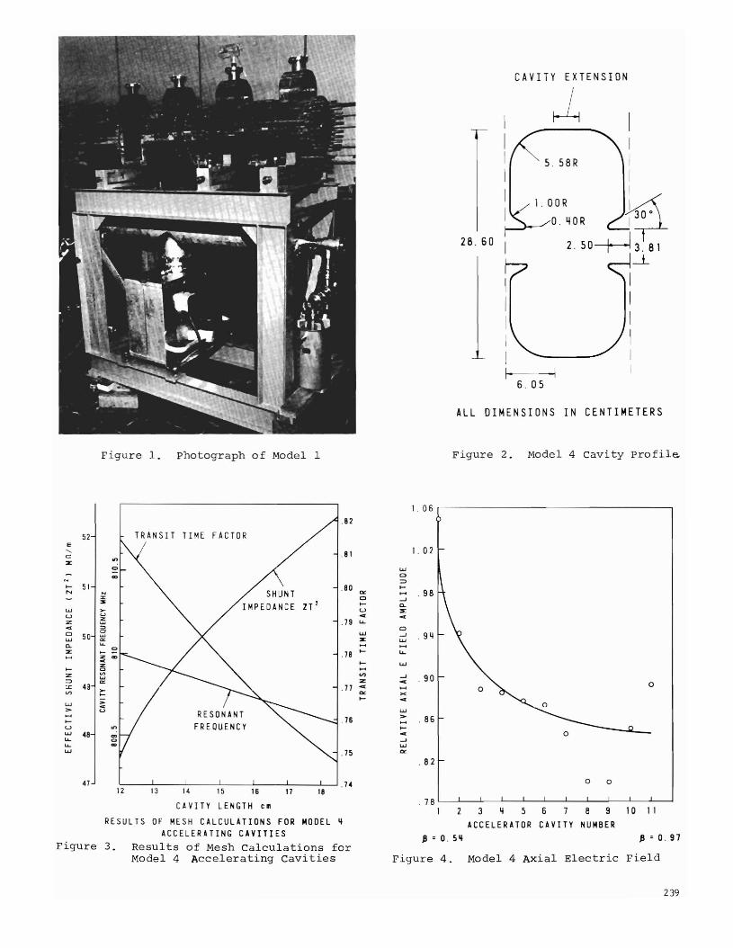
Model 4 is designed for aninjection energy of 96 keV (~=.54) andan output of 1.37 MeV (~=.96). Thelarge velocity change means that thecavity lengths must be increased tomaintain synchronism. The acceleratorcavity profile is shown in Fig. 2.Variation in cavity length is accomplishedby adding straight sections of differentlengths in the centre of the cell. Thereason for this construction is histori­cal. The copper segments used hadoriginally been machined for a ~=.65

tank. Fortunately, the cavity resonantfrequency is quite insensitive to thelength of extension, as can be seenfrom the graph of frequency versus cavitylength in Fig. 3. Thus the design of agraded-~ tank using these segments wasrelatively simple.

All the graphs in Fig. 3 pertainto the cavity profile in Fig. 2, and wereobtained from field calculations usingthe numerical mesh program SAMINT­OPOPSCAN (3).

The design of the graded-~ tankwas generated by a cell by cell energygain calculation for the synchronousparticle, in a manner similar to that1

Model 4 Accelerating Cavity Design

output PowerCavity Design Average Electron Dissipation

Cavity No. Length Axial Field Energy Per Cellmetres MV/m keV kW

1 0.1147 1.20 196 2.302 0.1370 1.13 306 2.223 0.1505 1.09 420 2.154 0.1591 1.07 536 2.105 0.1649 1.05 654 2.056 0.1691 1.04 772 2.037 0.1721 1.03 892 2.008 0.1744 1.03 1012 1.989 0.1762 1.02 1131 1.98

10 0.1776 1.02 1252 1.9611 0.1787 1.01 1373 1.95

233

used for design of Alvarez tanks.

Unequal accelerator cavity sizescombined with equal side coupler slot sizeslead to coupling factors and hence fieldamplitudes that vary from cell to cell.The magnitude of the field tilt was deter­mined empirically from a simple three cellmodel, and taken into account in thedesign. Fig. 4 shows the axial fieldamplitude along the tank. The solid curvecorresponds to the design while the plottedpoints were measured in the completed tank.Table 1 summarizes some of the designvalues for the accelerating cells of Model 4.

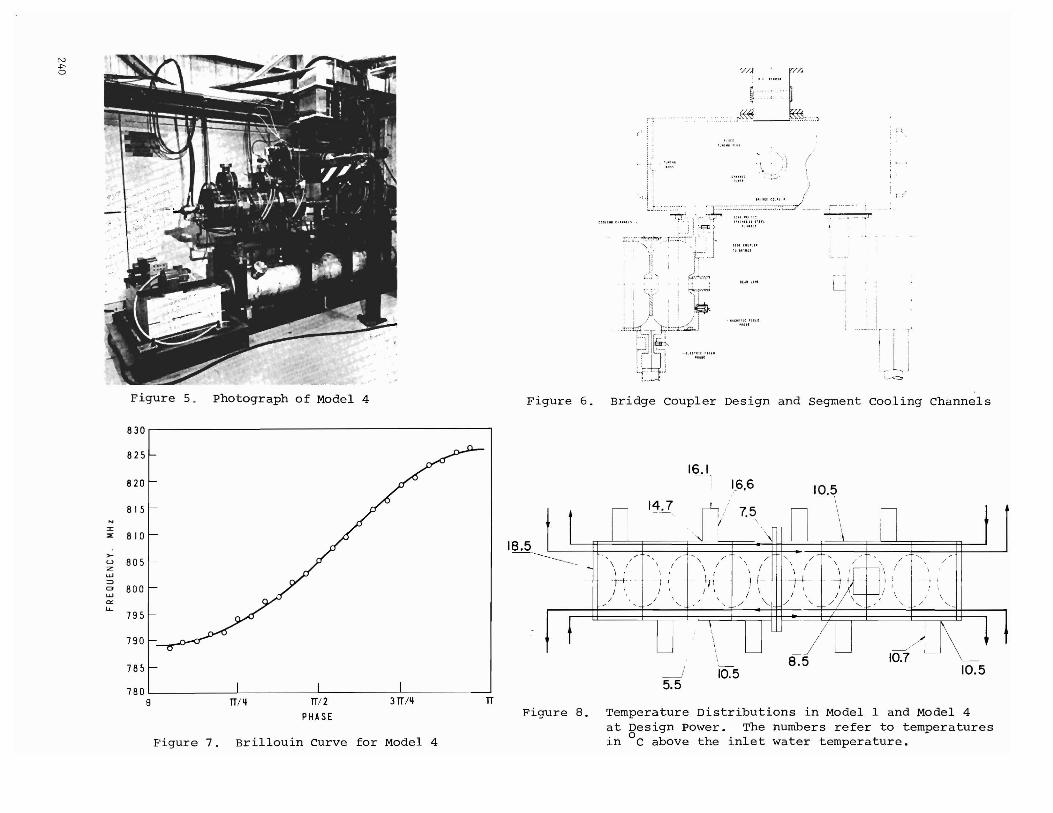
Fig. 5 is a photograph of theModel 4 tank prior to installation ofshielding. The tank was built in twosections each about 1 meter long, andjoined by a bridge coupler 80 cm long.Rf power is coupled to the tank through aniris in the bridge.

Attachment of the bridge to theaccelerator sections was made by an edge­weld seal at the centre of the sidecouplers adjacent to the bridge asillustrated in Fig. 6. Also shown are theaccelerator cavity cooling channels whichdiffer from those of Modell. In thiscase, prior to final assembly, two circum­ferential slots were machined into eachsegment and a cover brazed over them toform the cooling channels. Better thermalcoupling to the region of maximum powerdissipation is achieved in this way.

Tuning

Accelerating cell segments andcoupling cavities were tuned prior tofinal brazing. The tuning was done inthree steps; 1) segment tuning, 2) couplertuning, 3) coupling constant adjustment.

In the case of Model I, thesegments were tuned by clamping them sep­arately between copper plates in apneumatic press. The resonant frequencyof the two half cavities so formed wasmeasured to determine the amount of copperto be removed from the drift tUbe nose.After two or three machining operationsthe cavity frequencies were brought within100 kHz of the required tune value. Forthe purposes of this measurement the twohalf cavities were electrically isolatedby metal plugs in the beam hole and ashorting plate in the coupling slot.

Couplers were tuned by a combinationof machining copper from the capacitiveloading bosses and adjusting the distancebetween the bosses with a specially

234

designed jig. Their resonant frequencieswere determined by clamping them in turnonto a segment in the tuning press andmeasuring the 0, rr/2 and rr-mode fre­quencies and then calculating thecoupler frequencies using the usualcoupled circuit model (4).

Coupling constants were checkedafter brazing of the couplers to thesegments by measuring the two modefrequencies of a coupler and half cellwith the other half cell of the segmentdetuned. Only small adjustments werenecessary to equalize the couplingconstants to within 1%.

The tuning of Model 4 whilediffering in detail followed thegeneral procedure above. Because thistank is terminated in full cellshowever, it was necessary to tune theseterminating cavities 1 MHz lower than theothers to achieve minimum field in theside couplers.

After final brazing the Q values forModell and Model 4 were 24,400 and 23,350respectively. Both models showed a de­crease in the rr/2 mode frequency ofapproximately 0.5 MHz after brazing.Fitting of a Brillouin curve to themode spectrum showed that second neighbourcoupling had increased significantly.possible origin of these changes are:

1) Sagging of the coupling slotduring brazing

2) Cavity frequency shift becauseof improved rf contact at thebraze joints

3) Braze alloy flow from the segmentjoint into the vicinity of thecoupling slot.

Boroscope examination showed that suchalloy flow did occur in some cells.

The Brillouin curve for Model 4is shown in Fig. 7. The alternate highand low deviations of the measuredfrequencies from the fitted curve, nearthe ends of the curve, appear to berelated to the break in periodicitycaused by the bridge coupler. No suchdeviations were observed when the twotank sections were measured separately,but a similar behaviour has been noted inanother bridge coupled tank, built forthe Electron Test Accelerator.

Testing Facilities

Radiofrequency System

Two klystrons were used at varioustimes in the high power tests of the struc­tures viz, a 100 kW klystron (VA-853M) anda high efficiency 100 kW klystron (VA-3076).All were operated with the normal serviceinterlocks for vacuum and water flow. Afast protect system was used to detect andannunciate excessive forward or reversepower transients, rf arcs at the klystronwindow and excessive body current. Thesesignals remove the drive power to theklystron in less than 1 ~sec. If thealarm condition persists for longer than30 ~sec a crowbar system is triggered toremove the dc voltage from the tube. Rfarcs at the klystron window or excessivebody current produce an unconditionalcrowbar.

The low power drive system consistsof a voltage-programmable stable oscillator,fixed attenuator, isolator, diode switchand directional coupler feeding 10 mW ofrf power to a transistorized 30 db class Camplifier. The klystrons are generallyrun unsaturated and the drive power of0-10 watts is provided through a voltageprogrammable PIN modulator.

The klystrons were commissioned bydumping the power into a flat water load.Calorimetric measurements of efficiencywere taken and with careful tuning at805 MHz, efficiencies of 53% for theVA-853M and 65% for the VA-3076 wereachieved at 100 kW. It was found howeverthat the klystrons behaved more stablyalthough at lowered efficiency when tunedat broader bandwidths of around 7 MHz.

Driving into resonant loads at highpower imposes considerable demands on therf control systems. Our approach to thesolution of some of these problems aremore fully discussed elsewhere (1). Inthe experiments discussed here a highpower isolator having an insertion lossof 0.3 db and reverse attenuation of3.8 db was used to provide some toleranceto excursions from resonance. Our reversepower trip was set at 2 kW by a signaltaken from a WR-975 waveguide directionalcoupler protecting the klystron.

Tank Resonance Control

It was initially planned to provideresonance control of Modell through itscooling water temperature. This provedunsuccessful. We decided therefore toexperiment with control of the tank

resonant frequency using a mechanicaltuner in the bridge of Model 4 for fastcontrol while the cooling system regulatesthe water temperature to provide slowresonance control only. Experiments havebeen performed with Model 4 to keep thefrequency fixed by using the bridgetuning plunger to compensate for thermalchanges at high power. Results ofthese experiments are presented else­where.

All high power tests describedbelow were performed with a constantinlet water temperature. The klystrondrive frequency was controlled by anautomatic frequency controller whichadjusted the frequency of the masteroscillator to the resonant frequency ofthe tank. The controller operates byfrequency modulating the drivefrequency with a 10 kHz signal, giving amaximum frequency deviation of 1.5 kHz,and then detecting the resulting ampli­tude modulation of the cavity fieldswith a crystal detector. The demodulatedcavity signal and the 10 kHz modulatingsignal are combined in a phase sensitivedetector circuit to produce the feedbackcontrol signal.

Structure Properties at High Power

Tank commissioning

For the Model 1 tests an arcdetector was used to trip the klystronpower in addition to the vacuum, radiationand cooling water flow trips used byModel 4. Initial attempts to run thetanks by gradually increasing the cwpower led to numerous klystron tripsfrom arcs, reverse power and poorvacuum. The latter was presumably due tomultipactoring. Even after the tankshave been run at high cw power for longperiods a recommissioning procedure isrequired before the structures willsupport again the design fields of1 MV/m.

A satisfactory conditioning pro­cedure was developed as follows. Atvery low average power the tank ispulsed to high peak power for approximat­ely 20 ~sec at a fixed resonantfrequency. An RC filter is set at 30~sec so that the reverse power peaks atthe beginning and end of the pulse donot activate the reverse power trips.Usually the tank pressure increases froma base level of around 10-7 torr to 10-6

torr during this cleaning process. Whenthe tank vacuum improves the pulse width

235

is increased until the average powerceases to become negligible, resulting ina change of the tank resonant frequency.At this point the rise and fall time of thepulse fed to the PIN modulator in the kly­stron drive line is increased to a fewmilliseconds. This operation usuallygives rise to multipactor resonances whichagain increase the tank pressure. Aftersome hours the frequency of multipactoringdecreases and when it disappears the basepressure is regained. At this point cwoperation can begin. Recently an isolatorproviding 17.5 db of reverse powerattenuation, when the ferrites are cold,has been installed. The ability to with­stand larger arc induced impedance mis­matches at low duty factors will allowmore rapid tank conditioning in the future.

Temperature Distributions

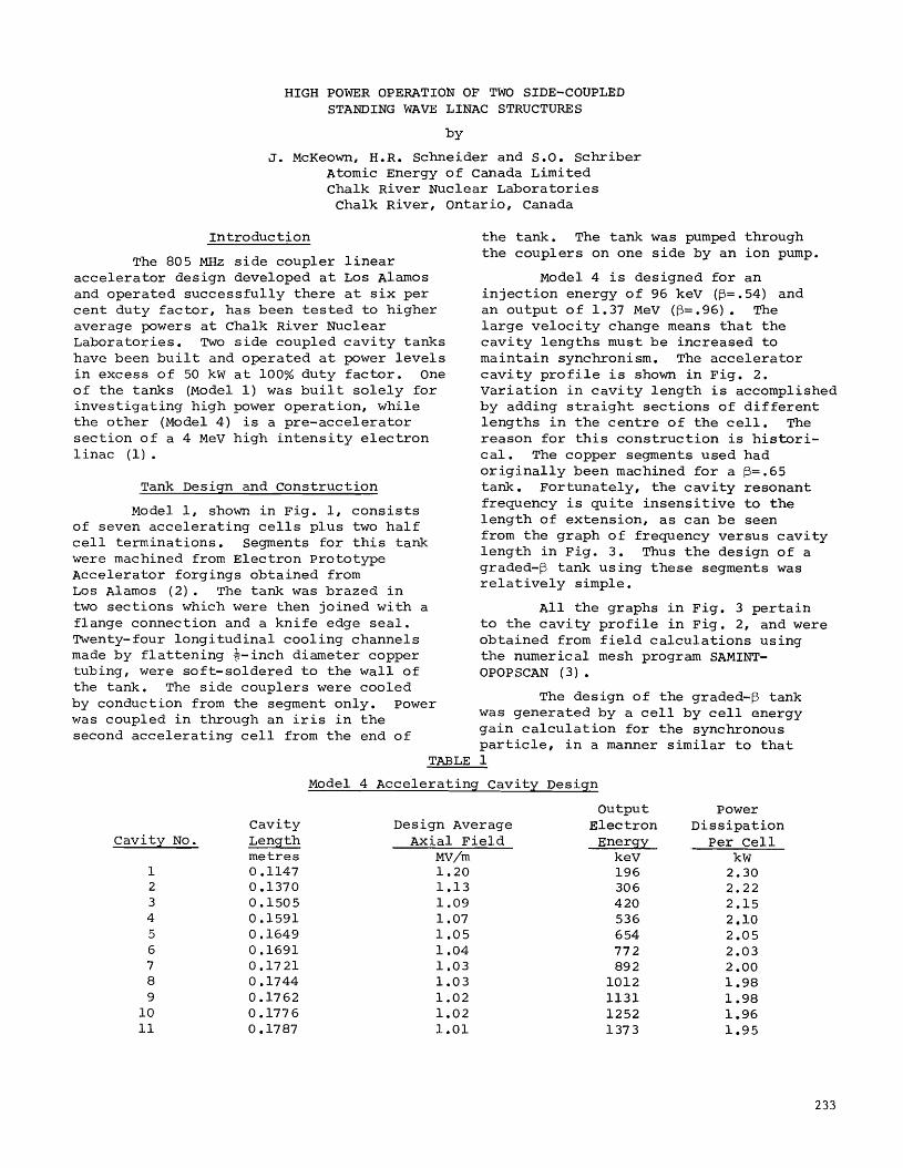
structure de-tuning will occurthrough thermal expansion of the structure.Of particular interest is the temperaturedistribution in the septum between twoaccelerating cells. A numerical cal­culation (5) of the temperature gradient inthe Modell cavities was compared withmeasurements taken at two different pene­trations of two cells when a net power of20 kW (2.5 kW/cell) was supplied to thestructure. The depths and temperaturesshown in Table 2 are measured relative tothe outer surface.

sistent with a calculated value of 219.8kHz for Modell. Measurements were alsomade of the frequency changes at zero powerresulting from changes in the averagetemperature. The thermal sensitivity ofthe ~/2 mode frequency was found to be-13.6 kHz/oC consistent with the thermalexpansion of copper.

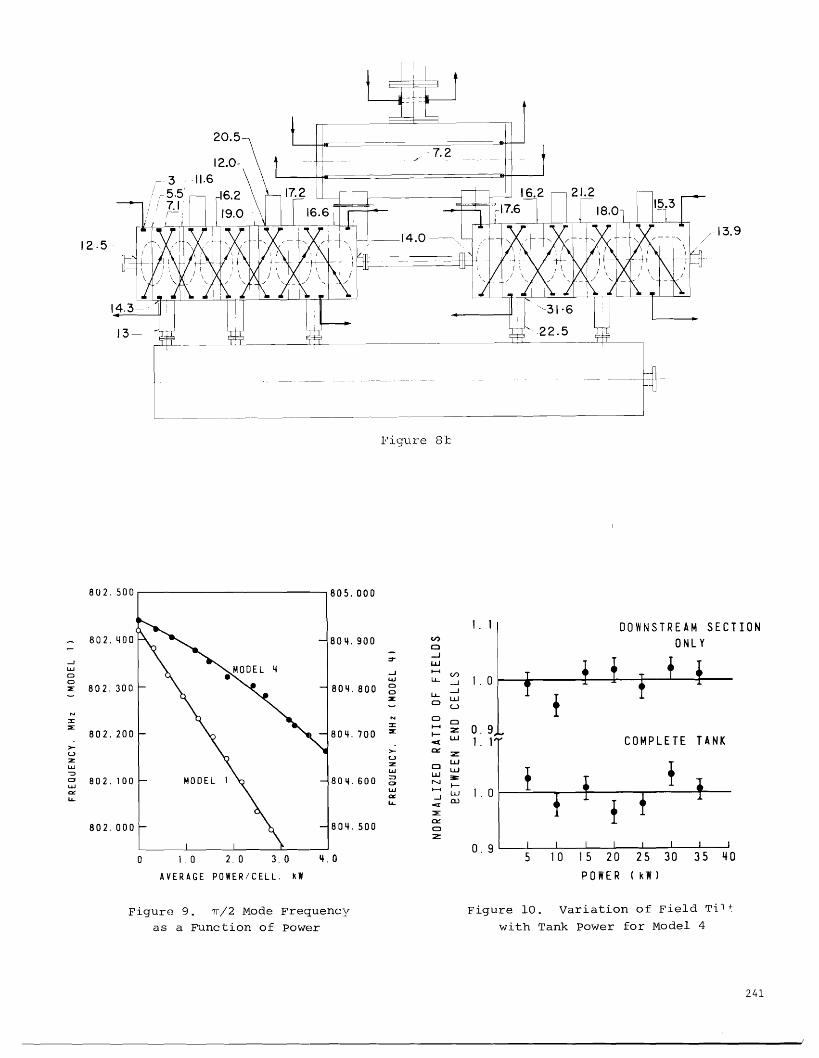
The physical distortion of the cellprofile at high power decreases the ~/2

mode frequency. This decrease is dueprimarily to the expansion at the highelectric field point of the acceleratingcell nose. For both tanks the frequencydecreases almost linearly with power asshown in Fig. 9. In Modell the dropin frequency is constant at 158 kHz/kW/cell. Of this, 68 kHz/kW/cell comes fromthe increase in the ambient temperature ofthe walls and the remaining 90 kHz/kW/cell is assumed to come from profile dis­tortion. In Model 4 the total drop infrequency from both sources has an averagevalue of 87 kHz/kW/cell. The considerabledecrease in sensitivity of the lattertank to thermal changes caused by rfpower, demonstrates the superior heattransfer characteristics obtained bymachining the cooling channels into thetank structure.

Field Distributions

The Model 1 tank was coupled to

TABLE 2: septum Temperatures in Modell

Penetration intoseptum (cms)

MeshCalculation (oC)

MeasuredCell #1 Cell #7

8.3

5.7

22.2

7.8

Copper temperature distributionsrelative to the average cooling water temp­erature were measured for the design powersof 20 kw (2.5 kW/cell) and 32 kW (2.57/cellaverage) for Model 1 and Model 4 respect­ively. The data presented in Fig. 8 showthe copper temperatures relative to theinlet cooling water temperature.

Rf Performance at High Power

(i) Frequency changes

Frequency increases attributed tothe change in the dielectric constant withremoval of dry nitrogen from the tanks werefound to be 222 kHz and 201 kHz for Model 1and Model 4 respectively. This is con-

236

give a low power VSWR of 1.04. Thematch changes smoothly from a slightlyundercoupled condition to a slightlyovercoupled condition with increase inpower. In Model 4 an overcoupled matchof 1.15 was achieved through a circulariris in the bridge of 9.65 cms indiameter. There is some structure in thereverse power curve in going from low tohigh power at 100% duty factor. This maybe due to small discharges which do notseem to occur when the klystron is pulsedat very low average power.

Fig. 10 shows the variation offield tilt with tank power for Model 4.The results have been normalised to

consider only the ratio of signals from thefield probes located at the opposite endsof the tank sections and the complete tank.The rms deviation from the mean field ratiois 2.4% for these data without evidence ofany systematic trend.

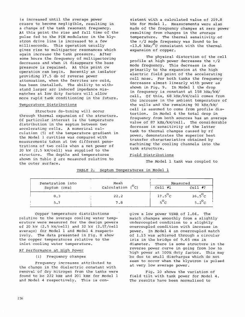
A more sensitive measure of the tankbehaviour is found from 'the side-couplerfields. A comparison of side couplerfields measured for both cw and pulsedoperation with a peak input power of 61.5kW in Model 1 and 32 kW in Model 4 showedwide variations. The results are givenin Table 3. These can only be accountedfor by changes in the cell-to-cell couplingand small changes in relative cell resonantfrequencies due to temperature differences.Model 4 does not show quite as large aspread as does Modell.

Resonant frequencies of modes otherthan the v/2 mode were measured at variousv/2 mode power levels. Power for thesemodes was obtained by driving one sidecoupler with a swept signal of 10 wattsand detecting in another coupler using anotch filter to suppress the ff/2 mode.A marker frequency from a stableoscillator was imposed on the sweptfrequency in order to measure accuratelythe mode frequencies. Th~ results of ananalysis of the mode frequencies using thecoupled circuit analog are shown inTable 4.

For both tanks the model shows theexpected trend of a decrease in resonantfrequency for both accelerating cells andside couplers. The first and secondneighbour coupling is independent of power

TABLE 3: Ratio of High Power cW/Pulsed Side Coupler Fields

CouplerNumber

123456789

1011

Model 161.5 kW 10% duty factor

0.3 ms pulse

cw field/pulsed field

1.550.251.571.411.442.490.701.02

Model 434 kW 1.2% duty factor!

3 ms pulse

cw field/pulsed field

1.140.660.570.820.931.31.30.960.831.071.2

TABLE 4~ Results from Mode Spectra Fit at Different Power Levels

I SecondII Nearest Nearest

v/2 Mode Accelerating I Side Coupler Neighbour Neighbour ! stopInput Power Cell Frequency I Cell Frequency

I

Coupling Coupling Band!

(kW) (MHz)I

(MHz) (MHz)! Constant constantModel 1

0 803.994 802.205 0.04456 -0.00395 0.2072.5 803.951 ! 802.164 0.04456 -0.00392 0.215

I

3 803.902 ! 802.117 0.04456 -0.00394 0.208

I

15 803.720 I 801.889 0.04457 -0.00394 0.25420 803.588 ! 801.766 0.04458 -0.00395 0.239

I Model 40 806.878 I 804.841 0.04503 -0.00484 0.0935 806.841 804.787 0.04507 -0.00483 0.112 I

15 806.802 i 804.681 0.04496 -0.00490 0.15225 806.686

I804.561 0.04507 -0.00480 0.197

I

32 806.619 804.488 0.04506 -0.00474 0.225

237

for Modell. For Model 4 the second neigh­bour coupling peaks slightly at inter­mediate powers but the results are notconclusive. For both tanks the stop bandincreases with power, significantly forModel 4.

The results for both tanks aresurprising as one would expect the acceler­ating cell frequencies to change at agreater rate than the side couplers withchanges in power. The coupled circuitanalysis will provide a better analog tostructure behaviour for the Model 1 tankthan the Model 4 tank. For the latter tankthe model provides only an average of thecoupling constants. Also the bridge inModel 4 with its consequent lack of secondneighbour coupling and the full end cellsdisturbs the symmetry of the model. It isnevertheless somewhat surprising that themodel indicates larger coupler frequencyshifts than accelerating cell frequencyshifts at high power for both tanks.

The phase differences between firstand last cells was less than 0.7

0from zero

power to 20 kW for Modell. From coupledloop model calculations these differenceswould imply less than ± 1.5% changes inrelative axial field changes. The phasechanges for Model 4 were greater but aclearly defined systematic trend was ob­served. When the power was increased froma calorimetrically measured power of 6 kWto 39 kw the low energy end of the structuredecreased in phase by 1.3

0relative to the

high energy end of the structure.

Model 4 Beam Test

In a preliminary run a beam of250 ~A was accelerated through Model 4 andstopped in a copper Faraday cup immediatelyafter the final cell. The average beamenergy was determined from radiation andcalorimetric measurements to be (1.24 ± 0.1MeV) for a net power of 24.1 kW. Thededuced value for the effective shuntimpedance (ZT2), assuming a synchronousphase angle of 26

0, is 67.7 ~ 8 MO, or

24% below the value of 88.3 MO calculatedfor the case with couplers and couplingslots neglected.

Conclusion

The side coupled linear acceleratordesign developed at Los Alamos has beentested up to axial fields of 1.6 MV/m with100% duty factor. The structures arestable at these power levels and have beenused to accelerate a test electron beam to

238

1.34 MeV at average axial fields of 1.1Mv/m. Under these conditions the axialelectric field tilts are less than 2.4%and the phase changes were found to differoby 1.3 from low power measurements.

Milling the cooling channels intothe segment structure reduces detuning athigh power. Lack of water cooling in theside couplers is a weakness in the presentdesigns and coupler cooling channelsshould be incorporated in future tanks tobe used at high power.

Acknowledgements

We are indebted to S.B. Hodge whowas responsible for the mechanical designof the tanks.

References

(1) liThe Chalk River Electron TestAccelerator ll J.S. Fraser, S.H. Kidner,J. McKeown and G.E. MCMichael,paper this conference.

(2) IIDesign and Initial Performance of a20 MeV High Current Side CoupledCavity Electron Accelerator ll

E.A. Knapp and W.J. Shlaer, Proceed­ings of 1968 Proton Linear Acceler­ator Conference (BNL 50120) p. 635.

(3) o. Aboul-Atta and A. Malecki,private communication.

(4) IIStanding Wave High Energy Acceler­ator Structures ll E.A. Knapp,B.C. Knapp, and J.M. Potter, Reviewof Scientific Instruments ~' 979,(1968) .

(5) CAVE, a program to calculate temp­erature distributions in linaccavities, J. Griffiths, privatecommunication.

6. 05

5. 58 R

CAVITY EXTENSION

IIII

,----,--' 000: OR h12B.60 I 2. 50~ 3.81

-i.

I

IIIII

ALL DIMENSIONS IN CENTIMETERS

Figure 1. Photograph of Modell Figure 2. Model 4 Cavity Profile

.82

52 TRANSIT TIME FACTORE.....

.81c:::0:

<;>

II)

0- 51 .80N N SHUNT IX

:I: 0::IE

IMPEDANCE ZT! 0-w >- uu u ...z ~ .79 LL« ::>0 0 UJ50 ~

w '" :::0:0.. ~ .....:::0: .78 0-.....

0-0- .....Z V)

OJ :z::<: 4a . 77 ...V) ~ IX

>-0-

W ..>- u.....

.760-uUJ 48LLLLw .75

47 .7412 13 14 15 16 17 18

CAVITY LENGTH CIII

RESULTS OF MESH CALCULATIONS FOR MODEL IIACCELERATING CAVITIES

Figure 3. Results of Mesh Calculations forModel 4 Accelerating Cavities

1. 06

1.02

w0OJ0-..... · 98--'0..:::0:...0--' · 911w.....LL

UJ

--' · 90... 0.....><...w>- · 860-... 0--'UJor:

.82

o 0

· 781 2 3 II 5 6 7 8 9 10 11

ACCELERATOR CAVITY NUMBERIJ = O. 511 IJ = O. 97

Figure 4. Model 4 Axial Electric Field

239

]",:··r.f"' ....._k

, ,

,-

~ I- _,

"'~.-<:::o

; .

i.....L.!c ..· r ..~'

I ! :1 t iI I I~-_... L,.J

.~_~~~_~~ .!l ..• i I

, I IL_)

I---ILj

i

(",\

W",)

'''<:r ~,i:rC~;0.::;:j-Jf ~ J.~~.;~

1\ '~r";, ~ : I' i"i..l,,',

,i j:i' ~__±-)..,/ '" i ; ; I'

"+' -r- h ,.;;±.......!'~J ~~_..~- .....[tg,

1 _",,,,,,,,,,.I "...

~ _. _.J

N-!'­o

Figure 6. Bridge Coupler Design and Segment cooling Channels

10.510.7

I "-

1\ / \ /. LI \

I ·--1I \ i \

" \ ....

1..6.6

10.5

16.1-,I

-..l5.5

\\ ,·t·-j- .. ·I '

I

Figure 8. Temperature Distributions in Model 1 and Model 4at Design Power. The numbers refer to temperaturesin °c above the inlet water temperature.

IT

Figure 5. Photograph of Model 4

830

825

820

815N

:r::l[ 810

>-(J 805zw:::>a 800w

'"LL.

795

790

785

7808 TTl'! TTl 2 3ITI'!

PHASE

Figure 7. Brillouin Curve for Model 4

I

Figure 8t

COMPLETE TANK

DOWNSTREAM SECTIONONLY

1. 0 \----=:....-__-...-+---....,.....-----llf--

1. 0 f-----:IIiI~--_+_--±--~---L--1---

O. 9 L..--.l_----L_----l.._--l.-_......L..-_...L--_L-----J

5 10 15 20 25 30 35 40

POWER (kW)

1.1

0.91.1

Figure 10. Variation of Field Ti 1 +

with Tank Power for Model 4

802. 500 ...---------------....... 805. 000

802.400 804.900 <.I)

a~

.J-' L.LJw

-' .....-.t0 (/)

0 w l.J... -l::::E 802.300 804.800 0

0 .J::::E

l.J... L.LJ0 U

:t: 0 a::::E :t: .....-.t :z:802.200 804. 700 ::::E I- L.LJ>-

cru >- ex :z:z u

L.LJw z a-=> w

UJL.LJ

C3 B02.100 804.600 ::JN

~

W 0 r-D' w ........

L.LJ..... D' -'..... <[OJ

~

802.000 804.500ex0:z:

a 1. a 2. 0 3.0 ~.O

AVERAGE POWER/CELL. kW

Figure 9. Tr/2 Mode Frequencyas a Function of Power

241