Embed Size (px)
Citation preview
1/34
High Precision Pulsar Timing with PINT a newsoftware package
Jing Luo
University of Toronto
March 21, 2019PyGamma19
2/34
Outline
I PulsarsI Pulsar timing with PINT
I Pulse time of arrival (TOA)I Modeling TOAsI Updating timing modelI Applications
I Future plans
3/34
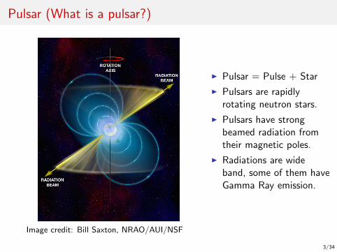
Pulsar (What is a pulsar?)
I Pulsar = Pulse + Star
I Pulsars are rapidlyrotating neutron stars.
I Pulsars have strongbeamed radiation fromtheir magnetic poles.
I Radiations are wideband, some of them haveGamma Ray emission.
Image credit: Bill Saxton, NRAO/AUI/NSF
4/34
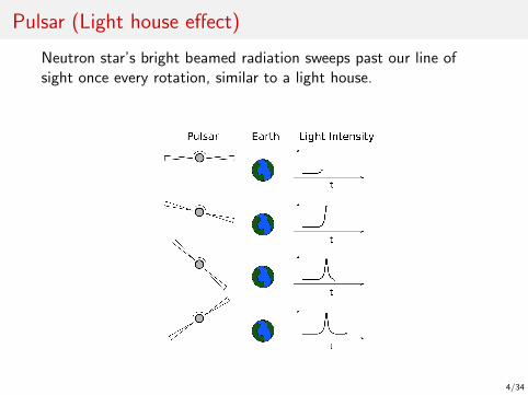
Pulsar (Light house effect)
Neutron star’s bright beamed radiation sweeps past our line ofsight once every rotation, similar to a light house.
Figure 1
5/34
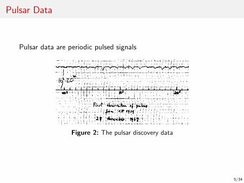
Pulsar Data
Pulsar data are periodic pulsed signals
Figure 2: The pulsar discovery data

6/34
Pulsar Data in pop culture
Figure 3: Pulses from CP1919 aliened with their period

7/34
Pulsar data at high energy
Figure 4: An example of PSR b1957+20 Fermi data.
8/34
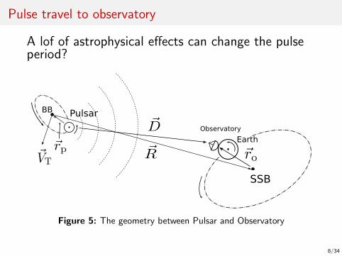
Pulse travel to observatory
A lof of astrophysical effects can change the pulseperiod?
SSB
Earth
Observatory
BB Pulsar
Figure 5: The geometry between Pulsar and Observatory

9/34
Pulsar Timing with PINT
Pulsar Timing with PINT

10/34
Pulsar Timing
Pulsar timing is a technique of modeling astrophysical phenomena(e.g., pulsar emission and propagation) via the pulse time ofarrivals (TOAs)
I Pulsar timing process
Figure 6
11/34
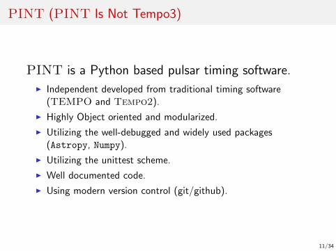
PINT (PINT Is Not Tempo3)
PINT is a Python based pulsar timing software.
I Independent developed from traditional timing software(TEMPO and Tempo2).
I Highly Object oriented and modularized.
I Utilizing the well-debugged and widely used packages(Astropy, Numpy).
I Utilizing the unittest scheme.
I Well documented code.
I Using modern version control (git/github).
12/34
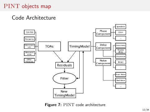
PINT objects map
Code Architecture
Figure 7: PINT code architecture
13/34
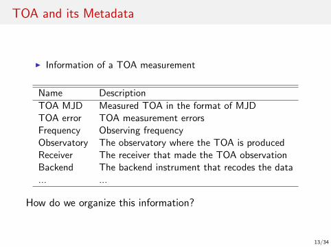
TOA and its Metadata
I Information of a TOA measurement
Name Description
TOA MJD Measured TOA in the format of MJDTOA error TOA measurement errorsFrequency Observing frequencyObservatory The observatory where the TOA is producedReceiver The receiver that made the TOA observationBackend The backend instrument that recodes the data... ...
How do we organize this information?
14/34
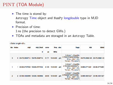
PINT (TOA Module)
I The time is stored by:Astropy Time object and NumPy longdouble type in MJDformat.
I Precision of time:1 ns (the precision to detect GWs.)
I TOAs and metadata are storaged in an Astropy Table.
15/34
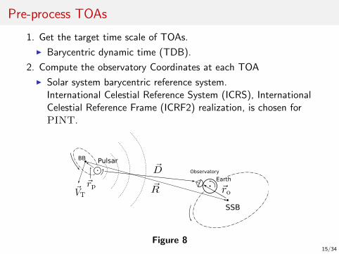
Pre-process TOAs
1. Get the target time scale of TOAs.
I Barycentric dynamic time (TDB).
2. Compute the observatory Coordinates at each TOA
I Solar system barycentric reference system.International Celestial Reference System (ICRS), InternationalCelestial Reference Frame (ICRF2) realization, is chosen forPINT.
SSB
Earth
Observatory
BB Pulsar
Figure 8
16/34
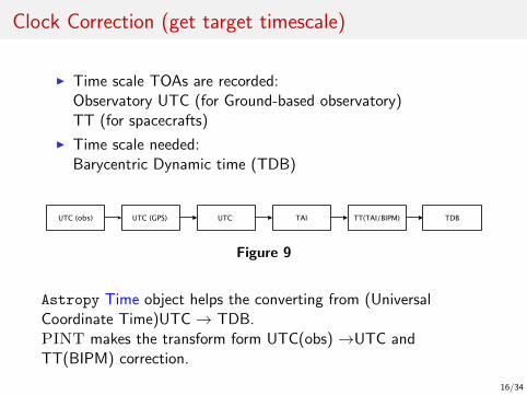
Clock Correction (get target timescale)
I Time scale TOAs are recorded:Observatory UTC (for Ground-based observatory)TT (for spacecrafts)
I Time scale needed:Barycentric Dynamic time (TDB)
Figure 9
Astropy Time object helps the converting from (UniversalCoordinate Time)UTC → TDB.PINT makes the transform form UTC(obs) →UTC andTT(BIPM) correction.
17/34
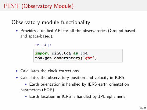
PINT (Observatory Module)
Observatory module functionality
I Provides a unified API for all the observatories (Ground-basedand space-based).
I Calculates the clock corrections.
I Calculates the observatory position and velocity in ICRS.
I Earth orientation is handled by IERS earth orientationparameters (EOP).
I Earth location in ICRS is handled by JPL ephemeris.
18/34
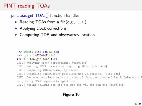
PINT reading TOAs
pint.toas.get TOAs() function handles:
I Reading TOAs from a file(e.g., .tim)
I Applying clock corrections.
I Computing TDB and observatroy location.
Figure 10
19/34
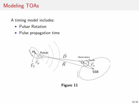
Modeling TOAs
A timing model includes:
I Pulsar Rotation
I Pulse propagation time
SSB
Earth
Observatory
BB Pulsar
Figure 11

20/34
Timing Model (Pulsar Rotation)
Modeling pulsar rotationUnder the pulsar co-moving frame
N(te) = N0 + ν0(te − t0) +1
2ν̇0(te − t0)2 +
1
6ν̈0(te − t0)3 + . . . , (1)
Notation Parameter Description
N0 ... Reference phaset0 ... Reference timete ... Pulse emission timeν0 F0 Spin frequencyν̇0 F1 Time derivative of spin frequencyν̈0 F2 Second order spin frequency derivative
However, the pulses are observed at the observatory.
te = tobs −∆, (2)
∆ is pulse propagation time.
21/34
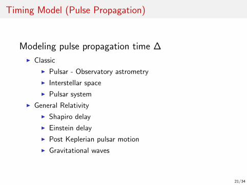
Timing Model (Pulse Propagation)
Modeling pulse propagation time ∆
I Classic
I Pulsar - Observatory astrometry
I Interstellar space
I Pulsar system
I General Relativity
I Shapiro delay
I Einstein delay
I Post Keplerian pulsar motion
I Gravitational waves
22/34
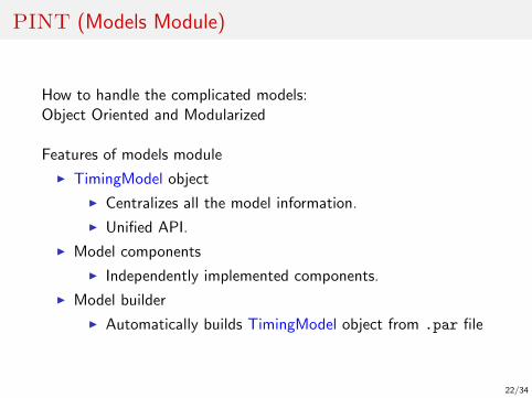
PINT (Models Module)
How to handle the complicated models:Object Oriented and Modularized
Features of models module
I TimingModel object
I Centralizes all the model information.
I Unified API.
I Model components
I Independently implemented components.
I Model builder
I Automatically builds TimingModel object from .par file
23/34
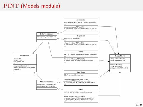
PINT (Models module)
24/34
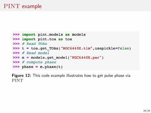
PINT example
Figure 12: This code example illustrates how to get pulse phase viaPINT
25/34
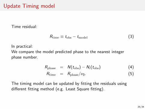
Update Timing model
Time residual:
Rtime ≡ tobs − tmodel (3)
In practical:We compare the model predicted phase to the nearest integerphase number.
Rphase = N(tobs)− Ni (tobs) (4)
Rtime = Rphase/ν0. (5)
The timing model can be updated by fitting the residuals usingdifferent fitting method (e.g. Least Square fitting).
26/34
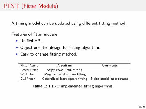
PINT (Fitter Module)
A timing model can be updated using different fitting method.
Features of fitter module
I Unified API.
I Object oriented design for fitting algorithm.
I Easy to change fitting method.
Fitter Name Algorithm Comments
PowellFitter Scipy Powell minimizing ...WlsFitter Weighted least square fitting ...GLSFitter Generalized least square fitting Noise model incorporated
Table 1: PINT implemented fitting algorithms
27/34
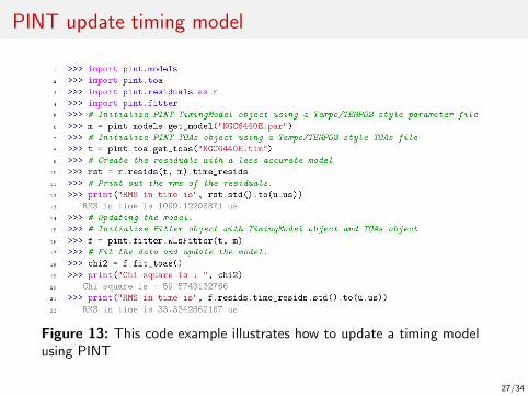
PINT update timing model
Figure 13: This code example illustrates how to update a timing modelusing PINT
28/34
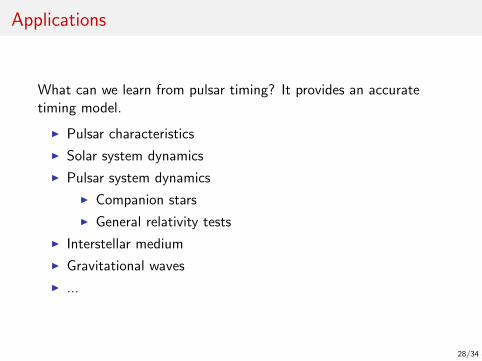
Applications
What can we learn from pulsar timing? It provides an accuratetiming model.
I Pulsar characteristics
I Solar system dynamics
I Pulsar system dynamics
I Companion stars
I General relativity tests
I Interstellar medium
I Gravitational waves
I ...
29/34
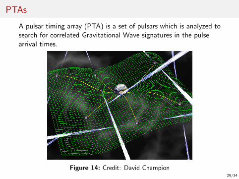
PTAs
A pulsar timing array (PTA) is a set of pulsars which is analyzed tosearch for correlated Gravitational Wave signatures in the pulsearrival times.
Figure 14: Credit: David Champion
30/34
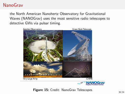
NanoGrav
the North American Nanohertz Observatory for GravitationalWaves (NANOGrav) uses the most sensitive radio telescopes todetective GWs via pulsar timing.
Figure 15: Credit: NanoGrav Telescopes

31/34
Current Status
I PINT is able to process NANOGrav 11-year data set.
I A set of high energy data analysis scripts and tools areprovided.
I PINT package has been adopted by:
I NANOGrav collaboration
I NASA’s NICER mission
I PINT is incorporated with gravitational wave analysispipelines.
I PINT is used to analyze NANOGrav 12.5-year data.
32/34
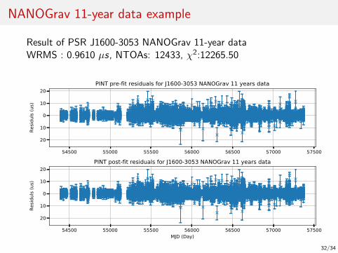
NANOGrav 11-year data example
Result of PSR J1600-3053 NANOGrav 11-year dataWRMS : 0.9610 µs, NTOAs: 12433, χ2:12265.50
54500 55000 55500 56000 56500 57000 57500
−20
−10
0
10
20
Resid
uls (
us)
PINT pre-fit residuals for J1600-3053 NANOGrav 11 years data
54500 55000 55500 56000 56500 57000 57500MJD (Day)
−20
−10
0
10
20
Resid
uls (
us)
PINT post-fit residuals for J1600-3053 NANOGrav 11 years data
33/34
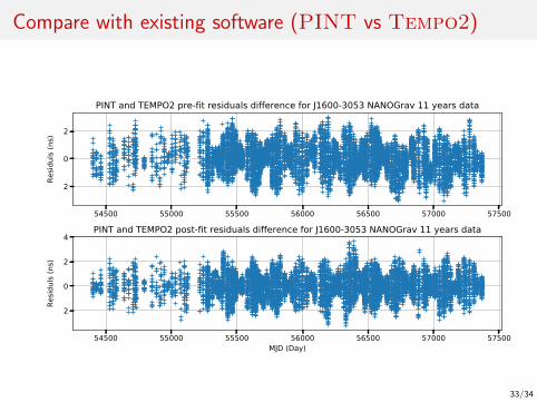
Compare with existing software (PINT vs Tempo2)
54500 55000 55500 56000 56500 57000 57500
−2
0
2
Resid
uls (
ns)
PINT and TEMPO2 pre-fit residuals difference for J1600-3053 NANOGrav 11 years data
54500 55000 55500 56000 56500 57000 57500MJD (Day)
−2
0
2
4
Resid
uls (
ns)
PINT and TEMPO2 post-fit residuals difference for J1600-3053 NANOGrav 11 years data
34/34
The Future
I PINT enables interactive pulsar data analysis and facilitatesthe pulsar tools development platform. (a lot of pulsar timingdata analysis tools will be based on PINT)
I PINT will be used as the major data analysis tool forNANOGrav 14-year data.
I PINT always welcome new features, new observatories, andPull request on Github: https://github.com/nanograv/PINT


![Pulsar Timing Analysis - Raman Research Institute · Pulsar Timing Analysis ... Event data file name[P2010_events_diffuse_gti.fits] ... TEMPO2 with Fermi plugin or manual entry of](https://img.pdfslide.net/doc/110x75/5b0c7f527f8b9a8b038c3b6c/pulsar-timing-analysis-raman-research-timing-analysis-event-data-file-namep2010eventsdiffusegtifits.jpg)