High-Precision Single-Frequency GPS Point Positioning

Tomas Beran, Donghyun Kim and Richard B. Langley

Geodetic Research Laboratory, Department of Geodesy and Geomatics Engineering, University of New Brunswick, Fredericton, New Brunswick, Canada

BIOGRAPHIES Tomas Beran received his Master’s degree in Surveying Science from the Czech Technical University in Prague in 1999. He is currently a Ph.D. candidate in the Department of Geodesy and Geomatics Engineering at the University of New Brunswick (UNB), where he is investigating the use of GPS for single-frequency precise point positioning. This research is being performed under the supervision of Professor Richard Langley at the department’s Geodetic Research Laboratory. Donghyun Kim is a research associate in the Department of Geodesy and Geomatics Engineering at the University of New Brunswick, where he has developed the UNB RTK software for a gantry crane auto-steering system. He has a B.Sc., M.Sc. and Ph.D. in geomatics from Seoul National University. He has been involved in GPS research since 1991. Currently, he carries out research related to ultrahigh-performance RTK positioning at up to a 50 Hz data rate, with application to real-time deformation monitoring, Internet-based moving platform tracking, and machine control. Richard Langley is a professor in the Department of Geodesy and Geomatics Engineering at the University of New Brunswick, where he has been teaching and conducting research since 1981. He has a B.Sc. in applied physics from the University of Waterloo and a Ph.D. in experimental space science from York University, Toronto. Professor Langley has been active in the development of GPS error models since the early 1980s and is a contributing editor and columnist for GPS World magazine. ABSTRACT The objective of the research described in this paper is to develop a Kalman filter-based functional model for single-frequency positioning which is suitable for low

dynamic platforms such as cars or boats. No external sensors are used and the precise velocity information comes from the time-differenced carrier-phase measurements. The Kalman filter combines these measurements with undifferenced code data to solve for user position, velocity, clock errors and major biases such as ambiguities. Utilizing the velocity information with range measurements provides fast convergence of the filter. The advantage over sequential least squares processing techniques is that it relies on an accurate model of the system dynamics. Imposing a near-constant acceleration constraint, we achieved high performance in terms of position accuracy by tuning the filter process noise parameters. Initial results from processing of geodetic-quality data show decimeter level accuracy, which is close to that of real-time standalone dual-frequency point positioning. Results of processing low-quality data are of similar accuracy, but they include biases due to multipath, residual atmospheric effects and some point positioning modeling considerations, which remain to be addressed. INTRODUCTION The precise point positioning technique is attractive to researchers because it does not require two or more simultaneously operating GPS receivers. It does not limit the solution success to a particular baseline length and it is suitable for various platforms. A number of research groups have demonstrated use of this technique for low earth orbiter position determination. Recent precise point positioning results show decimetre accuracy with use of dual-frequency geodetic-quality receiver [Bisnath and Langley, 2002]. High precision positioning results with a single GPS receiver can be obtained by use of precise GPS ephemerides and satellite clock offset information. Reliance on only single frequency measurements makes the solution more challenging, due to the ionospheric

delay estimation. To make the technique suitable for low-cost GPS hardware, we focused our research on extending this approach to single-frequency positioning. In this paper, our precise point positioning technique will be reviewed as well as Kalman filter techniques for various platforms. Data testing and conclusions will indicate strengths and weaknesses and the direction of future research. Precise Point Positioning Recent single point positioning concepts enhance pseudorange-based positioning with carrier-phase processing. Global networks of geodetic-quality GPS receivers providing precise GPS satellite orbits and precise satellite clock offset estimates allow for single point positioning. Single-receiver positioning functional models use pseudorange and carrier-phase measurements and data from global GPS networks. A carrier-phase-smoothed pseudorange processing technique was first proposed by Ron Hatch in the early 1980s [Hatch, 1982]. The carrier-phase and pseudorange combination uses averaged noisy code-phase range measurements to estimate the ambiguity term in the precise carrier-phase measurements. The longer the pseudorange smoothing, which requires continuous, cycle-slip-free, carrier-phase measurements, the better the carrier-phase ambiguity estimate. Point positioning modelling considerations include relativistic GPS satellite clock correction due to the eccentricity of GPS satellite orbits; GPS satellite phase centre to centre of mass offset; GPS satellite phase wind-up due to the relative rotation of the GPS satellite antennas with respect to receiver antenna; sub-diurnal variations in Earth rotation; solid Earth tides; ocean loading; and consistency between models used in the generation of GPS orbits and clocks and models used in the point positioning processing [Bisnath and Langley, 2002]. The UNB3 tropospheric prediction model [Collins, 1999] is used to correct for the most of the tropospheric delay. The omission of residual zenith delay estimation causes, on average, approximately few centimetre-level biases in the position estimates. Improved positioning results could be obtained with such estimation. FILTER MODELS AND SOLUTIONS The Kalman filter is usually used in variety of estimation processes, because it utilizes all measurements and dynamic information up to the current epoch. Single frequency pseudorange and carrier-phase measurements

are combined in the Kalman filter in a way that would optimize the use of information content of both types of observables. The discrete Kalman filter system model (dynamic model) is given by:

1,11, −−− += kkkkkk wxΦx , , 1 , 1~ ( , )k k k kN− −w 0 Q (1) where kx is the system state at time kt ; 1, −kkΦ is the system transition matrix which relates the state at time

1−kt to the state at time kt . The system transition matrix is derived from a set of differential equations describing the system dynamics. 1, −kkw is the system noise vector.

, 1k k−Q is the process noise variance matrix. The Kalman filter measurement model is given by:

kkkk vxHz += , ~ ( , )k kNv 0 R (2) where kz is the measurement vector; kH is the linearized system design matrix; i.e. the matrix of partial derivatives of the measurements with respect to each of the state variables; and kv is the measurement noise vector. kR is the measurement noise variance-covariance matrix. The complete set of discrete Kalman filter equations and their solutions can be found in Gelb [1974]. To avoid iteration in the solution, the extended Kalman filter is usually employed. In the extended Kalman filter, linearization takes place about the filter’s best estimate of the state. The degree to which the user dynamics are constrained or predictable dictates the type of process model used. A GPS receiver clock process model and dynamic platform process models will be described.

Receiver Clock Model Two state parameters, which represent the phase and frequency errors in a GPS receiver are required in any GPS-based estimator [Axelrad and Brown, 1996]. This model says that we expect both the frequency and phase to random walk over a short period of time. The discrete process equations are given by:

1,11, −−− += kkckckkckc wxΦx (3) where:

=

− tddt

kc 1x ,

∆=− 10

11,

tkkcΦ

∆∆

∆∆+∆

==−

tStS

tStStSE

tdtd

tdtddtTcckkc

2

23][ 2

23

1, wwQ

The white noise spectral amplitudes dtS and tdS can be related to the Allan variance parameters [Brown and Hwang, 1992]. Spectral amplitudes dtS and dtS were chosen to represent an uncontrolled crystal oscillator. Pseudorange and Carrier-Phase Model A pseudorange and carrier-phase model has been investigated. Absence of a velocity observable in this system makes it more suitable for static positioning applications. In this case, receiver position and receiver clock terms must be estimated together with other nuisance parameters such as carrier-phase ambiguities and zenith ionospheric delays. If kinematic GPS data are processed with this type of filter, the uncertainty in the position state parameters prediction (the system noise matrix) would have to be large enough to accommodate changes in position. Uncertain state parameters cause large innovation (observed minus predicted measurement) values and therefore less smoothing in the filter. The corresponding dynamic model is given by the following equation:

1,11, −−− += kkSkSkkSkS wxΦx (4) where:

1[ ... ]T

S n ion ionx y z N N dt dt d d=x (5)

Sx is the system state vector which includes position, ambiguities for n satellites, receiver clock parameters and ionospheric delay parameters. The corresponding system transition matrix follows:

=

−

−−

1,

1,1,

kki

kkckkS

ΦΦ

IΦ (6)

with (3 ) x (3 )n n= + +I identity matrix, where n is the number of satellites; and 1,1, −− = kkckki ΦΦ . The system noise covariance matrix is:

, 1

( )

( )[ ]

p p

T a aS k k S S

c

i

S t

S tE−

∆ ⋅

∆ ⋅ = =

I

IQ w wQ

Q

(7)

where (3 x 3)p =I identity matrix, ( x )a n n=I identity matrix and

∆∆

∆∆

=−

tStS

tStS

ti

ii

kki

2

232

23

1,Q

where pS represents the spectral amplitude for the

position random process. pS for a static observer should theoretically be set to zero (random bias model), but this may inherently cause numerical problems. This could be the result of the error covariance matrix converging to zero, when the filter deals with infinitesimally small numbers after a prolonged duration of processing. A value which maximizes the smoothing of the position component estimates is used (random-walk model). The same theory could be applied to the dynamic model of the ambiguity parameters. Instead of treating carrier phase ambiguities as constants, the spectral amplitude for the ambiguity random process, aS , is set to a value which allows ambiguities to absorb some of the unmodelled biases, such as residual atmospheric biases and multipath effects. iS represents the spectral amplitude of the zenith ionospheric delay integrated random-walk model. The pseudorange and carrier-phase measurement model follows the form of Equation (2):

ksksksks vxHz += (8) where:

0

i ioi

sk i i

−=

−

P Pz

Φ Φ,

i i

o−P P are observed minus computed pseudoranges and

0i i−Φ Φ are observed minus computed carrier-phases

−=

0)(01...010)(01...00

EFhhhEFhhh

iz

iy

ix

iz

iy

ixi

ksH ,

i

xh , iyh , i

zh are the measurement partial derivatives with respect to the receiver position; F(E) are the broadcast model ionospheric delay mapping functions [ICD-GPS-200C, 1999];

=

Φi

iP

kseε

v ,

and iPe and i

Φε are the measurement errors associated

with iP and iΦ , respectively. Pseudorange and Time-Differenced Carrier-Phase Model A low dynamic system model is more suitable for platforms with near-constant or zero accelerations, such as cars or boats. Time-differencing of carrier-phase measurements eliminates the carrier-phase ambiguity parameters and provides a velocity observable to the filter. The corresponding dynamic model is given by the following:

111, −−− += kLkLkkLkL wxΦx (9)

where:

TL tddtzyxzyx ][=x (10)

Lx includes the user position, velocity and receiver clock

terms. The corresponding system transition matrix follows:

, 1

, 1

00 00 0

Lk k

ck k

∆t

−

−

⋅ =

I IΦ I

Φ (11)

with I a 3 x 3 identity matrix. The system noise matrix is:

3 2

2

, 1

( ) ( ) 03 2

[ ] ( ) ( ) 020 0

p p

TLk k L l p p

c

t tS S

tE S S t−

∆ ∆⋅ ⋅

∆

= = ⋅ ∆ ⋅

I I

Q w w I I

Q

(12)

The spectral amplitude of the position and velocity integrated random-walk model, pS , is set in the same way as in the pseudorange and carrier-phase model. If the dynamical uncertainty of the vehicle is large, filtering would not improve the navigation solution. The process noise parameters were tuned to obtain an optimal solution. The pseudorange and time-differenced carrier-phase measurement model follows:

kLkLkLkL vxHz += (13)

where:

0

i ioi

Lk i iδ δ

−=

−

P Pz

Φ Φ,

i i

o−P P are observed minus computed pseudorange

measurements and 0i iδ δ−Φ Φ are observed minus

computed time-differenced carrier-phase measurements.

0 0 0 1 0

0 0 0 0 1

i i ix y zi

sk i i ix y z

h h h

h h h

=

H ,

i

xh , iyh , i

zh are the measurement partial derivatives with respect to the receiver position.

=

Φi

iP

kse

δεv ,

and i

Pe and iΦδε are the measurement errors associated

with iP and iδΦ , respectively. The broadcast ionospheric delay model and associated parameter values (Klobuchar model) were used. This model reportedly corrects for at least 50% (r.m.s.) of the ionospheric delay [Klobuchar, 1996] Recent developments have been made in an attempt to include the ionospheric delay parameters in the pseudorange and time-differenced carrier-phase model functional model, in the same way as it was done in the pseudorange and carrier-phase model. These developments are not reported in this paper. Point positioning modelling considerations such as relativistic GPS satellite clock correction; GPS satellite phase wind-up; sub-diurnal variations in Earth rotation; solid Earth tides and ocean loading remain to be added to the functional model. DATA TESTING AND ANALYSIS A number of tests were conducted to justify the selection of various functional models. The initial version of the processing software, programmed in Matlab, was built to illustrate the performance of various types of filters on widely varying data types. Two cases of static data and one case of kinematic data testing will be presented. Static Data Testing with a High-Quality GPS Receiver The objective of the static data testing was to investigate the pseudorange and carrier-phase filter’s ability to estimate ambiguities together with the zenith ionospheric delay parameters and to test the performance of the filter against high-quality positioning results.

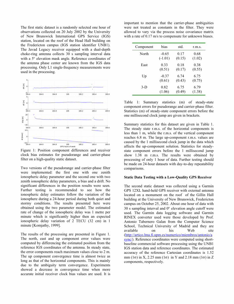
The first static dataset is a randomly selected one hour of observations collected on 20 July 2002 by the University of New Brunswick International GPS Service (IGS) station, located on the roof of the Head Hall building on the Fredericton campus (IGS station identifier UNB1). The Javad Legacy receiver equipped with a dual-depth choke-ring antenna collects 30 s sampling interval data with a 5° elevation mask angle. Reference coordinates of the antenna phase center are known from the IGS data processing. Only L1 single-frequency measurements were used in the processing.

164.4 164.6 164.8 165 165.2 165.4 165.6−5

0

5

dN [m

]

164.4 164.6 164.8 165 165.2 165.4 165.6−5

0

5

dE [m

]

164.4 164.6 164.8 165 165.2 165.4 165.6

−20

0

20

dUp

[m]

164.4 164.6 164.8 165 165.2 165.4 165.6−0.5

0

0.5

dt [m

sec]

GPS hours of week Figure 1: Position component differences and receiver clock bias estimates for pseudorange and carrier-phase filter on a high-quality static dataset. Two versions of the pseudorange and carrier-phase filter were implemented: the first one with one zenith ionospheric delay parameter and the second one with two zenith ionospheric delay parameters, a bias and a drift. No significant differences in the position results were seen. Further testing is recommended to see how the ionospheric delay estimates follow the variation of the ionosphere during a 24-hour period during both quiet and stormy conditions. The results presented here were obtained using the two parameter model. The estimated rate of change of the ionospheric delay was 1 metre per minute which is significantly higher then an expected ionospheric delay variation of 2 TECU (32 cm) in 1 minute [Komjathy, 1999]. The results of the processing are presented in Figure 1. The north, east and up component error values were computed by differencing the estimated position from the reference IGS coordinates of the antenna. In steady state, the error components reach maximum values close to 2 m. The up component convergence time is almost twice as long as that of the horizontal components. This is mainly due to the ambiguity term convergence. Experiments showed a decrease in convergence time when more accurate initial receiver clock bias values are used. It is

important to mention that the carrier-phase ambiguities were not treated as constants in the filter. They were allowed to vary via the process noise covariance matrix with a rate of 0.17 m/s to compensate for unknown biases.

Component bias std. r.m.s.

North -0.65 (-1.01)

0.17 (0.15)

0.68 (1.02)

East 0.33 (0.51)

0.18 (0.17)

0.38 (0.55)

Up -0.37 (0.61)

6.74 (0.43)

6.75 (0.75)

3-D 0.82 (1.06)

6.75 (0.49)

6.79 (1.38)

Table 1: Summary statistics (m) of steady-state component errors for pseudorange and carrier-phase filter. Statistics (m) of steady-state component errors before the one millisecond clock jump are given in brackets. Summary statistics for this dataset are given in Table 1. The steady state r.m.s. of the horizontal components is less than 1 m, while the r.m.s. of the vertical component reaches 6.8 m. The large up-component r.m.s. values are caused by the 1 millisecond clock jump in the data which affects the up-component solution. Statistics for steady-state component errors before the 1 millisecond jump show 1.38 m r.m.s. The results were obtained by processing of only 1 hour of data. Further testing should be made on 24-hour datasets with day-to-day repeatability comparisons. Static Data Testing with a Low-Quality GPS Receiver The second static dataset was collected using a Garmin GPS 12XL hand-held GPS receiver with external antenna located on a monument on the roof of the Gillin Hall building at the University of New Brunswick, Fredericton campus on October 25, 2002. About one hour of data with 30 s sampling interval and 0° elevation angle cutoff were used. The Garmin data logging software and Garmin RINEX converter used were those developed by Prof. Antonio Tabernero Galan from the Computer Science School, Technical University of Madrid and they are available on his Web site (http://artico.lma.fi.upm.es/numerico/miembros/antonio/async/). Reference coordinates were computed using short-baseline commercial software processing using the UNB1 IGS station data and reference coordinates. The estimated accuracy of the reference Cartesian coordinates is 1.52 mm (1σ) in X, 2.25 mm (1σ) in Y and 2.18 mm (1σ) in Z components, respectively.

The objective of this experiment was to process low-grade single-frequency GPS receiver data from a location which is known to have significant multipath disturbance (L1 pseudorange multipath plus noise observable r.m.s. from the UNAVCO teqc data quality checking software is 1.12 m). Two types of Kalman filter processing models were used: the pseudorange and carrier-phase filter and the pseudorange and time-differenced carrier-phase model.

136.7 136.8 136.9 137 137.1 137.2 137.3 137.4 137.5 137.6 137.7−10

0

10

dN [m

]

136.7 136.8 136.9 137 137.1 137.2 137.3 137.4 137.5 137.6 137.7−10

0

10

dE [m

]

136.7 136.8 136.9 137 137.1 137.2 137.3 137.4 137.5 137.6 137.7

−20

0

20

dUp

[m]

136.7 136.8 136.9 137 137.1 137.2 137.3 137.4 137.5 137.6 137.7180

200

220

240

dt [m

sec]

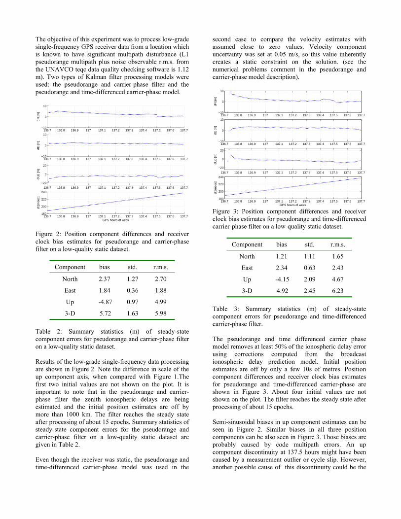
GPS hours of week Figure 2: Position component differences and receiver clock bias estimates for pseudorange and carrier-phase filter on a low-quality static dataset.

Component bias std. r.m.s.

North 2.37 1.27 2.70

East 1.84 0.36 1.88

Up -4.87 0.97 4.99

3-D 5.72 1.63 5.98 Table 2: Summary statistics (m) of steady-state component errors for pseudorange and carrier-phase filter on a low-quality static dataset. Results of the low-grade single-frequency data processing are shown in Figure 2. Note the difference in scale of the up component axis, when compared with Figure 1.The first two initial values are not shown on the plot. It is important to note that in the pseudorange and carrier-phase filter the zenith ionospheric delays are being estimated and the initial position estimates are off by more than 1000 km. The filter reaches the steady state after processing of about 15 epochs. Summary statistics of steady-state component errors for the pseudorange and carrier-phase filter on a low-quality static dataset are given in Table 2. Even though the receiver was static, the pseudorange and time-differenced carrier-phase model was used in the

second case to compare the velocity estimates with assumed close to zero values. Velocity component uncertainty was set at 0.05 m/s, so this value inherently creates a static constraint on the solution. (see the numerical problems comment in the pseudorange and carrier-phase model description).

136.7 136.8 136.9 137 137.1 137.2 137.3 137.4 137.5 137.6 137.7−10

0

10

dN [m

]

136.7 136.8 136.9 137 137.1 137.2 137.3 137.4 137.5 137.6 137.7−10

0

10

dE [m

]

136.7 136.8 136.9 137 137.1 137.2 137.3 137.4 137.5 137.6 137.7

−20

0

20

dUp

[m]

136.7 136.8 136.9 137 137.1 137.2 137.3 137.4 137.5 137.6 137.7180

200

220

240

dt [m

sec]

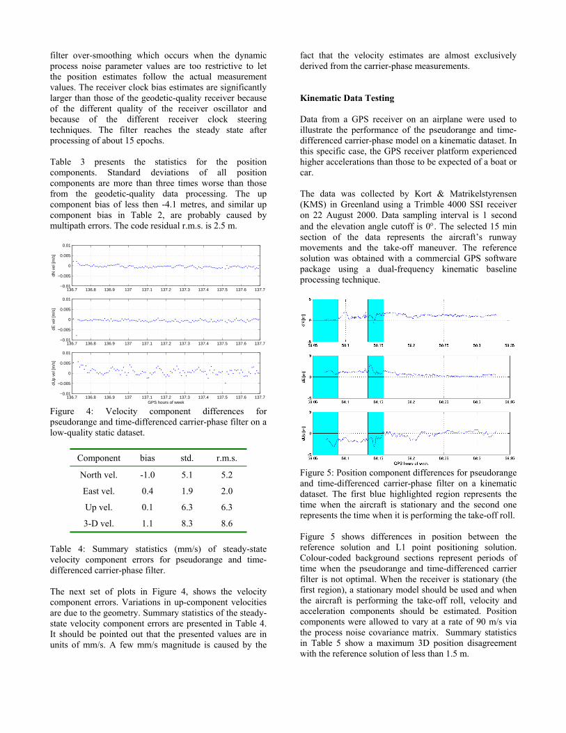
GPS hours of week Figure 3: Position component differences and receiver clock bias estimates for pseudorange and time-differenced carrier-phase filter on a low-quality static dataset.

Component bias std. r.m.s.

North 1.21 1.11 1.65

East 2.34 0.63 2.43

Up -4.15 2.09 4.67

3-D 4.92 2.45 6.23 Table 3: Summary statistics (m) of steady-state component errors for pseudorange and time-differenced carrier-phase filter. The pseudorange and time differenced carrier phase model removes at least 50% of the ionospheric delay error using corrections computed from the broadcast ionospheric delay prediction model. Initial position estimates are off by only a few 10s of metres. Position component differences and receiver clock bias estimates for pseudorange and time-differenced carrier-phase are shown in Figure 3. About four initial values are not shown on the plot. The filter reaches the steady state after processing of about 15 epochs. Semi-sinusoidal biases in up component estimates can be seen in Figure 2. Similar biases in all three position components can be also seen in Figure 3. Those biases are probably caused by code multipath errors. An up component discontinuity at 137.5 hours might have been caused by a measurement outlier or cycle slip. However, another possible cause of this discontinuity could be the

filter over-smoothing which occurs when the dynamic process noise parameter values are too restrictive to let the position estimates follow the actual measurement values. The receiver clock bias estimates are significantly larger than those of the geodetic-quality receiver because of the different quality of the receiver oscillator and because of the different receiver clock steering techniques. The filter reaches the steady state after processing of about 15 epochs. Table 3 presents the statistics for the position components. Standard deviations of all position components are more than three times worse than those from the geodetic-quality data processing. The up component bias of less then -4.1 metres, and similar up component bias in Table 2, are probably caused by multipath errors. The code residual r.m.s. is 2.5 m.

136.7 136.8 136.9 137 137.1 137.2 137.3 137.4 137.5 137.6 137.7−0.01

−0.005

0

0.005

0.01

dN v

el [m

/s]

136.7 136.8 136.9 137 137.1 137.2 137.3 137.4 137.5 137.6 137.7−0.01

−0.005

0

0.005

0.01

dE v

el [m

/s]

136.7 136.8 136.9 137 137.1 137.2 137.3 137.4 137.5 137.6 137.7−0.01

−0.005

0

0.005

0.01

dUp

vel [

m/s

]

GPS hours of week Figure 4: Velocity component differences for pseudorange and time-differenced carrier-phase filter on a low-quality static dataset.

Component bias std. r.m.s.

North vel. -1.0 5.1 5.2

East vel. 0.4 1.9 2.0

Up vel. 0.1 6.3 6.3

3-D vel. 1.1 8.3 8.6 Table 4: Summary statistics (mm/s) of steady-state velocity component errors for pseudorange and time-differenced carrier-phase filter. The next set of plots in Figure 4, shows the velocity component errors. Variations in up-component velocities are due to the geometry. Summary statistics of the steady-state velocity component errors are presented in Table 4. It should be pointed out that the presented values are in units of mm/s. A few mm/s magnitude is caused by the

fact that the velocity estimates are almost exclusively derived from the carrier-phase measurements. Kinematic Data Testing Data from a GPS receiver on an airplane were used to illustrate the performance of the pseudorange and time-differenced carrier-phase model on a kinematic dataset. In this specific case, the GPS receiver platform experienced higher accelerations than those to be expected of a boat or car. The data was collected by Kort & Matrikelstyrensen (KMS) in Greenland using a Trimble 4000 SSI receiver on 22 August 2000. Data sampling interval is 1 second and the elevation angle cutoff is 0°. The selected 15 min section of the data represents the aircraft’s runway movements and the take-off maneuver. The reference solution was obtained with a commercial GPS software package using a dual-frequency kinematic baseline processing technique.

Figure 5: Position component differences for pseudorange and time-differenced carrier-phase filter on a kinematic dataset. The first blue highlighted region represents the time when the aircraft is stationary and the second one represents the time when it is performing the take-off roll. Figure 5 shows differences in position between the reference solution and L1 point positioning solution. Colour-coded background sections represent periods of time when the pseudorange and time-differenced carrier filter is not optimal. When the receiver is stationary (the first region), a stationary model should be used and when the aircraft is performing the take-off roll, velocity and acceleration components should be estimated. Position components were allowed to vary at a rate of 90 m/s via the process noise covariance matrix. Summary statistics in Table 5 show a maximum 3D position disagreement with the reference solution of less than 1.5 m.

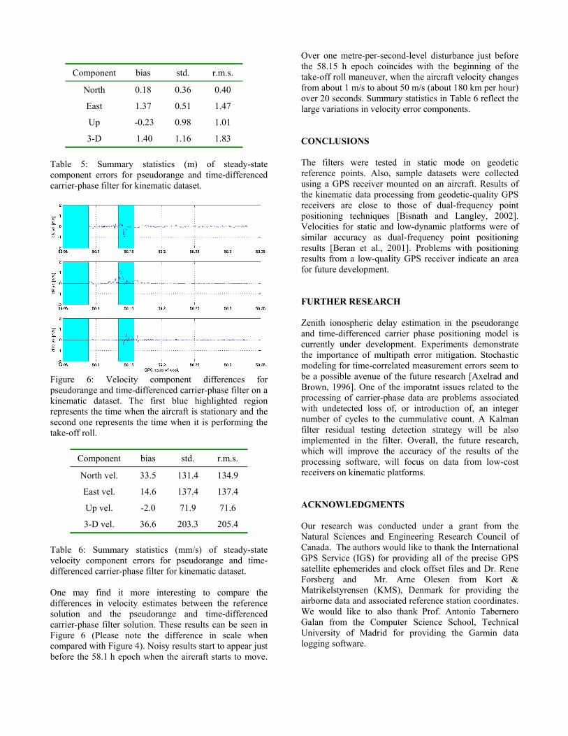
Table 5: Summary statistics (m) of steady-state component errors for pseudorange and time-differenced carrier-phase filter for kinematic dataset.

Figure 6: Velocity component differences for pseudorange and time-differenced carrier-phase filter on a kinematic dataset. The first blue highlighted region represents the time when the aircraft is stationary and the second one represents the time when it is performing the take-off roll.

Component bias std. r.m.s.

North vel. 33.5 131.4 134.9

East vel. 14.6 137.4 137.4

Up vel. -2.0 71.9 71.6

3-D vel. 36.6 203.3 205.4 Table 6: Summary statistics (mm/s) of steady-state velocity component errors for pseudorange and time-differenced carrier-phase filter for kinematic dataset. One may find it more interesting to compare the differences in velocity estimates between the reference solution and the pseudorange and time-differenced carrier-phase filter solution. These results can be seen in Figure 6 (Please note the difference in scale when compared with Figure 4). Noisy results start to appear just before the 58.1 h epoch when the aircraft starts to move.

Over one metre-per-second-level disturbance just before the 58.15 h epoch coincides with the beginning of the take-off roll maneuver, when the aircraft velocity changes from about 1 m/s to about 50 m/s (about 180 km per hour) over 20 seconds. Summary statistics in Table 6 reflect the large variations in velocity error components. CONCLUSIONS The filters were tested in static mode on geodetic reference points. Also, sample datasets were collected using a GPS receiver mounted on an aircraft. Results of the kinematic data processing from geodetic-quality GPS receivers are close to those of dual-frequency point positioning techniques [Bisnath and Langley, 2002]. Velocities for static and low-dynamic platforms were of similar accuracy as dual-frequency point positioning results [Beran et al., 2001]. Problems with positioning results from a low-quality GPS receiver indicate an area for future development. FURTHER RESEARCH Zenith ionospheric delay estimation in the pseudorange and time-differenced carrier phase positioning model is currently under development. Experiments demonstrate the importance of multipath error mitigation. Stochastic modeling for time-correlated measurement errors seem to be a possible avenue of the future research [Axelrad and Brown, 1996]. One of the imporatnt issues related to the processing of carrier-phase data are problems associated with undetected loss of, or introduction of, an integer number of cycles to the cummulative count. A Kalman filter residual testing detection strategy will be also implemented in the filter. Overall, the future research, which will improve the accuracy of the results of the processing software, will focus on data from low-cost receivers on kinematic platforms. ACKNOWLEDGMENTS Our research was conducted under a grant from the Natural Sciences and Engineering Research Council of Canada. The authors would like to thank the International GPS Service (IGS) for providing all of the precise GPS satellite ephemerides and clock offset files and Dr. Rene Forsberg and Mr. Arne Olesen from Kort & Matrikelstyrensen (KMS), Denmark for providing the airborne data and associated reference station coordinates. We would like to also thank Prof. Antonio Tabernero Galan from the Computer Science School, Technical University of Madrid for providing the Garmin data logging software.

Component bias std. r.m.s.

North 0.18 0.36 0.40

East 1.37 0.51 1.47

Up -0.23 0.98 1.01

3-D 1.40 1.16 1.83

REFERENCES Axelrad, P. and R.G. Brown (1996). “GPS Navigation

Algorithms.” In Global Positioning System: Theory and Applications Volume 1, Eds. B.W. Parkinson, J.J. Spilker Jr., Progress in Astronatics and Aeronautics Volume 164, American Institute of Aeronautics and Astronautics, Inc., Washington, D.C., U.S.A., pp. 409-433.

Beran, T., S.B. Bisnath and R.B. Langley (2001). “Single Receiver GPS Positioning in Support of Airborne Gravity for Exploration and Mapping.” Poster presented at the GEOIDE 3rd Annual Conference, Fredericton, June 20-22, 2001.

Bisnath, S.B. and R.B. Langley (2002). “High Precision, Kinematic Positioning with a Single GPS Receiver.” Navigation; Journal of The Institute of Navigation, Vol. 49, No. 3, Fall 2002, pp. 161-169.

Brown, R.G. and P.Y.C. Hwang (1983). “A Kalman Filter

Approach to Precission GPS Geodesy.” Navigation; Journal of The Institute of Navigation, Vol. 30, No. 4, Winter 1983-1984, pp. 338-349.

Brown, R.G. and P.Y.C. Hwang (1990). “GPS Navigation: Combining the Pseudorange with Continuos Carrier-Phase using a Kalman Filter.” Navigation; Journal of The Institute of Navigation, Vol. 37, No. 2, Summer 1990, pp. 181-196.

Brown, R.G. and P.Y.C. Hwang (1992). Introduction to

Random Signals and Applied Optimal Estimation. 2nd ed., Wiley, New York, 502 pp.

Collins, J.P. (1999). Assessment and Development of the

Tropospheric Delay Model for Aircraft Users of the Global Positioning System. M.Sc.E. thesis, Department of Geodesy and Geomatics Engineering Technical Report No. 203, University of New Brunswick, Fredericton, New Brunswick, Canada, 174 pp.

Gelb, A. (Ed.) (1974). Applied Optimal Estimation. The

MIT Press, Massachusetts Institute of Technology, Cambridge, 374 pp.

Hatch, R. (1982), “The Synergism of GPS Code and Carrier Measurements.” Proceedings of the Third International Geodetic Symposium on Satellite Doppler Positioning, Las Cruces, New Mexico, U.S.A., 8-12 February 1982, Vol. II, pp. 1213-1232.

ICD-GPS-200C (1999). Navstar GPS Space Segment/Navigation User Interface Control Document, ARINC Research Corporation, 138 pp.

Klobuchar, J. A. (1996). “Ionospheric Effects on GPS.” in Gobal Positioning System: Theory and Applications Volume 1, Eds. B.W. Parkinson, J.J. Spilker Jr., Progress in Astronautics and Aeronautics Volume 164, American Institute of Aeronautics and Astronautics, Inc., Washington, D.C., U.S.A., pp. 485-514.

Komjathy, A. (1999). Global Ionospheric Total Electron

Content Mapping Using the Global Positioning System. Ph.D. dissertation, Department of Geodesy and Geomatics Engineering Technical Report No. 188, University of New Brunswick, Fredericton, New Brunswick, Canada, 248 pp.