High-Resolution Imaging Without Iteration: A Fast and Robust Method for

Breast Ultrasound Tomography

P. Huthwaite

Department of Mechanical Engineering

Imperial College London

SW7 2AZ,

UK

F. Simonetti

School of Aerospace Systems

University of Cincinnati

Cincinnati

OH 45221,

USA

(Dated: June 16, 2011)

High-resolution breast tomography 1

Abstract

Breast ultrasound tomography has the potential to improve the cost,

safety and reliability of breast cancer screening and diagnosis over the

gold-standard of mammography. Vital to achieving this potential is the

development of imaging algorithms to unravel the complex anatomy of

the breast and its mechanical properties. The solution most commonly

relied upon is Time-of-Flight Tomography but this exhibits low res-

olution due to the presence of diffraction effects. Iterative full-wave

inversion methods present one solution to achieve higher resolution,

but these are slow and are not guaranteed to converge to the cor-

rect solution. Presented here is HARBUT, the Hybrid Algorithm for

Robust Breast Ultrasound Tomography, which utilises the complemen-

tary strengths of Time-of-Flight and Diffraction Tomography resulting

in a direct, fast, robust and accurate high resolution method of recon-

structing the sound-speed through the breast. The algorithm is shown

to produce accurate reconstructions with realistic data from a complex

3D simulation, with masses as small as 4mm being clearly visible.

PACS numbers: 43.80Qf, 43.60Pt, 43.20Fn

2

I. INTRODUCTION

Breast cancer is by far the most common cancer among women throughout the world,

with 411 000 deaths per year1. Breast cancer screening programmes, where women over the

age of 40 to 50 years have their breasts regularly checked for cancer, have been shown to

reduce death rates2,3. The current screening gold-standard is mammography, which projects

X-rays through the breast so that the absorption of the photons by the structures within

produces shadows which form an image. The detection of cancer is based on the assumption

that the cancer mass is denser – and hence absorbs more X-ray radiation – than the sur-

rounding tissue. The sensitivity (true positive rate) of the method is estimated at 68% to

88%4, but this drops to around 30% to 40% in radiographically dense breasts where struc-

tures within the breast – parenchyma and stroma – mask the presence of cancer masses.

Dense breast is a common occurrence, affecting approximately 50% of women under 50 years

and a third over5, and it is also in the latter group that the risk of developing cancer is the

highest.

There are two main diagnostic tools complementary to mammography that are now

routinely used in the clinic. The objective of these is to increase sensitivity and specificity

(true negative rate). Magnetic Resonance Imaging (MRI) is one method, producing accurate

images and achieving high sensitivity6. However, its use leads to a large number of unneeded

biopsies due to its low specificity7. Additionally the cost of examination is typically an order

of magnitude more expensive than mammography, and it relies on the injection of contrast

agents, making it unsuitable for widespread screening.

A second option used to aid diagnosis is sonography, which produces an image via a

handheld ultrasound array. Sonography is more sensitive in dense breasts than mammogra-

phy because it can distinguish between structures with similar density but different acoustic

impedance. However, being handheld, it is highly operator dependent and its use is limited

to situations where the areas of interest – an ambiguous mass for example – have already

been identified. This makes the technique in its current form unsuitable for screening.

3

Breast

Water

tankToroidal array

(a) (b)

x

y

x’

FIG. 1. Schematic of the system for breast ultrasound tomography. (a) The patient lies

prone with the breast suspended in a water tank. A transducer array begins at the chest

wall and gathers sets of data at many slices through the breast. Shown in (b) is a single

illumination and the scattered field produced which is measured by the transducer array.

We define x′ as a point inside the scatterer.

The possibility of improving the sensitivity and specificity of sonography has been inves-

tigated since the 1970s within the framework of breast Ultrasound Tomography (UST)8–15.

Thanks to recent progress in solid state electronics and array technology it is now possible

to replace handheld probes with automated systems11,12 such as the one shown in Fig. 1

which can produce full volume breast scans. The patient lies prone with the breast sus-

pended in the water bath and the array is repeatedly moved down to image slices through

it. At each slice, a single transducer provides an illumination, with the total field being

recorded around the breast. This process is repeated with the next transducer providing

the illumination and so on to provide a full matrix of scattering data for each vertical loca-

tion of the array. This matrix is then used to reconstruct the mechanical properties of the

materials within the breast with the goal of using these to distinguish cancer from healthy

tissue. Identifying the characteristic mechanical properties of cancer within the breast is

key to achieve high sensitivity and specificity. Greenleaf first proposed that cancer masses

are characterised by higher sound speed and attenuation than the surrounding medium16;

recent work is suggesting a similar pattern12.

The dominant approach in breast UST is Time-of-Flight Tomography (TFT)9,10,12,17–22

4

which applies a ray-based approach to arrival times for transmitted signals in order to

produce – either directly in the case of straight rays or with iterations for bent rays – a

sound-speed map. This follows the approach in X-ray CT based reconstruction systems

which can rely on simple straight ray approximations23,24. Diffraction effects are ignored

under this approximation and a measure of the achievable resolution is√Lλ where L is the

distance between transducer pairs and λ is the wavelength25–31. The size of a typical breast

limits the shortest λ to about 1mm to achieve full breast penetration and the minimum

distance between sensors L to about 200mm, thus resulting in a resolution in the region of

14mm. Although this should only be taken as an approximate estimation of the resolution

of TFT, it suggests that TFT is not suitable for imaging very fine structures in the breast.

Higher resolution imaging methods based on the Born or Rytov approximations, such

as Diffraction Tomography (DT)32–35, are suitable for imaging fine details of the breast

architecture. However, DT is of little use in breast imaging because the object to be imaged

must be of low contrast relative to the background and small relative to λ, such that the

maximum phase distortion through the object is much less than π, for the approximations

to be valid. The breast is a large object (around 50λ across at λ = 2mm) and the contrast

is high enough that the criterion for the validity of the approximation, as given in Ref. 34,

cannot generally be satisfied for breast UST.

An alternative solution being considered is to improve the resolution of the TFT image

with an iterative full-wave inversion technique36–38. The method uses the low resolution

TFT algorithm to reconstruct a starting model of the breast mechanical properties. The

algorithm then runs a numerical computer simulation to predict the signals that would be

measured with the system in Fig. 1 for this model. The target of the algorithm is to minimise

the residual between the resulting signal and the measured signal by updating the material

properties of the breast; the breast model that minimises the residual provides the final

image. The model refinement is generally achieved by a gradient-based stepping method.

The first issue with this technique is that the algorithm will only converge to the nearest

local minimum rather than the global minimum of the problem. Because of this, the starting

5

model – i.e. the image produced by the TFT algorithm – must already be close to the global

minimum. Also, the technique is susceptible to uncertainties not considered in the forward

model – for example transducer characteristics, 3D effects, and noise which can lead to the

the algorithm converging to an incorrect solution. Speed is another significant drawback:

a full set of illuminations needs to be simulated at each step (and more to calculate the

gradient) with many iterations needed to generate the final image.

This paper introduces HARBUT, the Hybrid Algorithm for Robust Breast Ultrasound

Tomography, which addresses the need for a fast, robust, high-resolution breast ultrasound

tomography method, by combining the complementary strengths of the TFT and DT al-

gorithms to reconstruct a sound speed map. The TFT image is used to correct for the

aberration that causes DT to break down under the Born approximation. A similar ap-

proach has already been introduced by Mast39, although this uses DT rather than TFT

as a background, limiting the contrast which can be imaged. Here, we provide an imaging

algorithm optimised for the circular array configuration in Fig. 1, and study how 3D features

close to the image plane affect the reconstructions. The latter point is of primary importance

because the circular array configuration is not ideal for 3D imaging which would require a

spherical aperture.

Sec. II describes the standard Born approximation upon which DT is based and modifies

it such that it forms the basis for the new algorithm. Sec. III presents the new imaging

method, and Sec. IV details the model and data that will be used to test it. Sec. V presents

the image reconstructions obtained with the new method and consideration to practical

implementation is given in Sec. VI.

II. SCATTERING THEORY

Here, we introduce a formulation for ultrasound scattering that provides the basis for

the imaging method presented in Sec. III.

The standard acoustic wave equation40 is the accepted model used to describe ultrasound

6

propagation in tissue

ρ(r)∇.[

1

ρ(r)∇p(r)

]

− 1

c(r)2∂2p(r)

∂t2= 0 (1)

where p(r) is the pressure at point r, ρ(r) is the density and c(r) is the sound speed. By

converting this to the temporal frequency domain it can be rewritten as

(∇2 + k2w)ψ = −Oψ (2)

where ψ is the scalar potential of the field (equal to the Fourier transform of the pressure)

and kw = 2πf/cw is the wavenumber of the water background where f is the frequency

and cw is the sound speed in water. Throughout this paper the homogeneous background

corresponds to the water bath (with subscript w), although these equations are valid for any

homogeneous background. The object function, O(r), is the mathematical representation of

the breast and is defined as

O(r) = k2w

[(

cwc(r)

)2

− 1

]

− ρ1/2(r)∇2ρ−

1/2(r) (3)

where c(r) is the actual sound speed at point r. The aim of tomography is to reconstruct

this object function. The second term in (3) accounts for variations in the local density field,

ρ41. The dependence of the density term on the Laplacian means that it is only significant

at an interface where rapid changes in density occur; this term will therefore be low away

from the boundaries within the breast and is considered negligible for the rest of this paper,

as will be explained in detail later in Sec. VI.

In order to solve (2) we define the water wave field ψw as the solution to the case where

there is no breast immersed in the water, and use the Green’s function in water Gw to reach,

under the Born approximation33,34

ψ ≈ ψw −∫

Ω

GwOψwdx′. (4)

For the Born approximation to be valid, the maximum phase distortion as waves pass

through the object must be less than π34. It is this that limits the applicability of the stan-

7

dard Born approximation imaging methods to breast UST – the breast is typically around

100mm (50λ at λ = 2mm) in diameter meaning that its sound speed contrast relative to

the water bath must be less than 1% to meet this criterion.

In this paper we address the phase distortion problem by dividing the object function

into a sum of an ‘artificial’ inhomogeneous background object function Ob, and a small

perturbation Oδ so that

O(r) = Ob(r) +Oδ(r). (5)

Using the same procedure as in standard DT33,34 we can derive the following integral

ψ = ψb −∫

Ω

GbOδψdx′ (6)

where Gb is the Green’s function defined for the inhomogenous background and ψb is the

illumination distorted by the background.

Provided Oδ is sufficiently small, under the integral we can approximate the ψ term with

the background term ψb so that

ψ ≈ ψb −∫

Ω

GbOδψbdx′ (7)

which is a more accurate version of (4). Equation (7) is central to the Distorted Born Iter-

ative Method (DBIM) that aims to solve the wave equation through an iterative scheme42.

For (7) to be sufficiently accurate the background medium has to be selected so as to ensure

that the phase difference between ψb and ψ is much less than π. This is the inhomogeneous

equivalent of the standard Born criterion as given in Ref. 34.

It is the combination of size and contrast of the bulk of the breast which breaks the

standard Born approximation. Provided we have a background that accounts for the average

speed through the breast then the sizes and contrast of the remaining perturbations should

be small enough that the Born approximation criterion given in Ref. 34 will be valid for

them. In this context, TFT provides a suitable background, as will be demonstrated in

Sec. V.

8

III. THE HARBUT METHOD

This section uses the formulation from the previous section as a basis for HARBUT. We

start from a particular implementation of DT that has been introduced in Ref. 43.

A. An implementation of DT

This method consists of two main steps: beamforming (BF) and the application of a

filter. We begin with the derivation of the beamforming algorithm.

We introduce the coordinates x and y as the coordinates of the receiver transducer and

source transducer respectively. x′ is defined as in Fig. 1. Using these, and defining the

scattered field as ψs = ψ − ψw, we can rewrite (4) as

ψs(x,y) ≈ −∫

Ω

Gw(x,x′)O(x′)ψw(y,x

′)dx′. (8)

We can demonstrate the symmetry of this equation by recognising that ψw(y,x′) = Gw(y,x

′)

i.e. the field produced by an illumination at y can simply be replaced by the equivalent

Green’s function. This leads to

ψs(x,y) ≈ −∫

Ω

Gw(x,x′)O(x′)Gw(y,x

′)dx′. (9)

Now consider a single point scatterer in a water background. In this case, the equation

is simplified from an integral to

ψs(x,y) = Gw(x,x′)qGw(x

′,y) (10)

where we have taken the scattering potential of the point as q, located at x′. Knowing

the location of the point scatterer we can rearrange (10) to determine the exact scattering

potential from a single scattering measurement, i.e.

q =ψs(x,y)

Gw(x,x′)Gw(x′,y). (11)

9

In this equation, it can be considered that the 1Gw

factors provide corrections to the scattered

field ψs so as to account for the phase shift and amplitude change as the wave propagates

through the medium. In general, however, the location of each scatterer is unknown, and

there are multiple scatterers present so that the signals interfere and make the use of (11)

unfeasible in its current form.

The solution considered here is to take advantage of the multiple send-receive pairs

in the data, rather than just the single pair as above. This is done in the beamforming

algorithm (also known as the sum and delay method or SAFT - Synthetic Aperture Focusing

Technique), which is performed in the time domain by applying a backwards time shift to

account for the shift that occurs as the wave propagates through the medium, and summing

up the results for each send-receive pair44–46. In the frequency domain, the time-shifts

correspond to the phase shifts of the Green’s functions, so that the image value at point z is

IBF∗(z) =

∫

S

∫

S

ψs(x,y)

sgn [Gw(x, z)] sgn [Gw(z,y)]dxdy (12)

where S is the aperture of the transducer array and the sign function is defined as sgn(x) =

x/|x| so that only the phase component of Gw is used. For real, sampled data the continuous

integrals are replaced by discrete sums. Due to this integral/summing process, if there is

a scatterer present at the imaging point then the integrand will sum coherently leading to

a large value, but if there is no scatterer at the point then the summing will be incoherent

and the result will be much weaker, with the values cancelling themselves out.

When quantitatively determining the scattering potential in Eq. (11), it is clearly nec-

essary to correct for both amplitude and phase changing as the wave travels through the

medium. Following this, we adjust Eq. (12) to use the full Green’s functions in the beam-

forming integrand, matching the form of Eq. (11), to give

IBF (z) =

∫

S

∫

S

ψs(x,y)

Gw(x, z)Gw(z,y)dxdy. (13)

Throughout this paper we use this version of the BF algorithm since by accounting for

amplitude we keep the algorithm more general. This would allow us, for example, to ac-

10

Scattering

dataBeamforming Filter

Object

function

pertrubation,

Oδ

Time-of-flight

TomographyOb

Original BF/DT algorithm

HARBUT

FIG. 2. Flowchart of the stages which make up the original BF/DT algorithm, and the

additional TFT stage which is included in HARBUT

count for background media which cause significant amplitude changes, for example through

attenuation.

As discussed in Ref. 43, the BF image is a distorted image of the DT reconstruction

with different weights applied to different spatial frequencies which generates a distorted

reconstruction. The DT reconstruction is obtained by correcting this weighting, which

is done by Fourier transforming the BF image, applying the weighting corrections, and

transforming the result back to the geometrical space. This approach is more flexible than

directly generating the DT image, and is essential for HARBUT, as presented in the next

section.

B. Combining DT and TFT

We now consider the case of imaging in an inhomogeneous background. This process

is similar to the homogeneous case, with the addition of the TFT algorithm to provide a

suitable background. Fig. 2 illustrates the process.

The first step is to perform the beamforming algorithm, this time accounting for the

background. Starting from (7), we substitute ψb = Gb and include the source and receiver

coordinates x and y

ψ(x,y) ≈ ψb(x,y)−∫

Ω

Gb(x,x′)Oδ(x

′)Gb(y,x′)dx′. (14)

11

We use a TFT image to provide the background sound speed field. In this paper we gen-

erate the TFT image by the method in Ref. 47, although the actual method used is not

critical to the success of the algorithm, provided it gives a reasonable low resolution recon-

struction of the sound-speed. The Green’s functions for this background field need to be

calculated via a numerical simulation, where each illumination is calculated separately to

provide wavefield values at all points in the imaging domain. An eikonal equation solver48

provides sufficiently accurate results throughout the domain, with significant speed advan-

tages over alternatives such as frequency domain finite difference; a secondary advantage of

using ray-approximation-based methods is that such solvers (and the solutions they provide)

are often already available as part of the TFT algorithm. The use of the eikonal solver is

a distinction between our algorithm and Ref. 39, which uses a simple straight-ray approxi-

mation; our algorithm is therefore better suited to cases where the breast causes significant

refraction. The numerical method is only used to provide a phase correction relative to the

Green’s function in homogeneous water bath, so that

Gb (x′,y) = G0 (x

′,y) eiω∆t (15)

where ∆t is the difference in arrival time between the propagation in the background model

and propagation in homogeneous water, calculated via the eikonal solver.

If we now consider a point scatterer in an inhomogeneous medium, we can follow through

exactly the same logic as in Sec. III.A except starting with (14) instead of (9) to give the

BF image of the perturbation relative to the background,

IBFδ (z) =

∫

S

∫

S

ψδ(x,y)

Gb(x, z)Gb(z,y)dxdy (16)

where ψδ = ψ − ψb is the perturbation of the measured field relative to the background.

Given that all of these quantities can be established, either from measurements or numerical

models, we can form the modified beamforming image from this equation. This is similar

in approach to the Kirchhoff migration method used in geophysics49. Kirchhoff migration is

only used on reflected data, however, and reconstructs the interfaces of impedance variations

12

in the subsurface rather than material properties. Similar work has been done in medical

imaging which again only reconstructs impedance variations13.

The BF image generated from (16) is then converted to the DT image using the filter

introduced in Ref. 43. This filter is given as a function of spatial frequency, Ω as

F (Ω) =kw|Ω|

√

1− |Ω|2/4k2w8π2Π

Λ(Ω) (17)

where

Λ (Ω) =

1, |Ω| < 2kw

0, |Ω| > 2kw.

Having obtained Oδ by filtering IBFδ , it is combined with the background velocity field

according to (3) and (5), forming the final HARBUT image. It should be observed that

HARBUT solves (7); this process corresponds to the first iteration of the DBIM42,50. How-

ever, our approach uses a different scheme to solve (7) based on the TFT starting model

and the combination of BF and DT. This combination represents the main novelty of the

method and is key to its robustness and speed, as discussed next.

Mast39,51 proposed a similar synthetic-aperture type method for reconstructing sound

speed maps while correcting for aberrations. However, this was only used for iterating from

a homogeneous starting point, rather than a TFT image, so its range of validity was only

about double that of the standard Born approximation. The contrast and size of the breast

– in general – is likely to be beyond this.

For the proposed method to be feasible in practice, it is necessary to consider the ex-

perimental constraints that affect the nature and accuracy of the measurements. In this

context, the main factors are:

1. 3D effects and sampling conditions. The array architecture shown in Fig. 1 is suitable

for imaging 2D objects. The anatomy of the breast is fully 3D which would require

a spherical array to perform all the measurements required to satisfy the Nyquist

sampling criterion. Therefore it is important to understand whether the reconstruction

can be treated as 2D and what type of artefacts one could expect as a result.

13

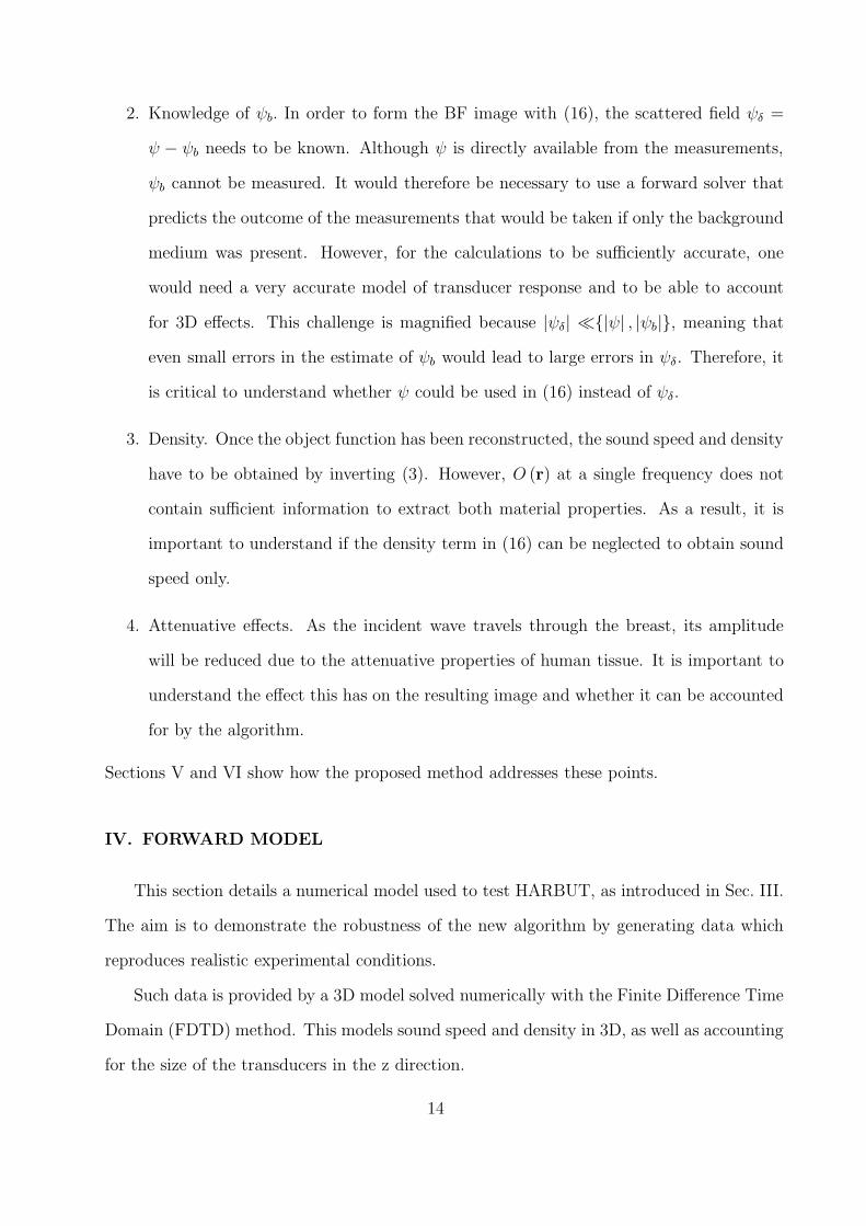
2. Knowledge of ψb. In order to form the BF image with (16), the scattered field ψδ =

ψ − ψb needs to be known. Although ψ is directly available from the measurements,

ψb cannot be measured. It would therefore be necessary to use a forward solver that

predicts the outcome of the measurements that would be taken if only the background

medium was present. However, for the calculations to be sufficiently accurate, one

would need a very accurate model of transducer response and to be able to account

for 3D effects. This challenge is magnified because |ψδ| ≪|ψ| , |ψb|, meaning that

even small errors in the estimate of ψb would lead to large errors in ψδ. Therefore, it

is critical to understand whether ψ could be used in (16) instead of ψδ.

3. Density. Once the object function has been reconstructed, the sound speed and density

have to be obtained by inverting (3). However, O (r) at a single frequency does not

contain sufficient information to extract both material properties. As a result, it is

important to understand if the density term in (16) can be neglected to obtain sound

speed only.

4. Attenuative effects. As the incident wave travels through the breast, its amplitude

will be reduced due to the attenuative properties of human tissue. It is important to

understand the effect this has on the resulting image and whether it can be accounted

for by the algorithm.

Sections V and VI show how the proposed method addresses these points.

IV. FORWARD MODEL

This section details a numerical model used to test HARBUT, as introduced in Sec. III.

The aim is to demonstrate the robustness of the new algorithm by generating data which

reproduces realistic experimental conditions.

Such data is provided by a 3D model solved numerically with the Finite Difference Time

Domain (FDTD) method. This models sound speed and density in 3D, as well as accounting

for the size of the transducers in the z direction.

14

A. Physical model

Selecting a suitable, realistic breast model is challenging since the necessary material

properties of the breast are difficult to measure and tend to vary from person to person. The

wide range in quoted values (see for example Refs. 52–54) reflects this variation. Therefore,

we use the more extreme, higher contrast values (which are more challenging to Born-

approximation-based algorithms) in order provide a thorough test of the new algorithm.

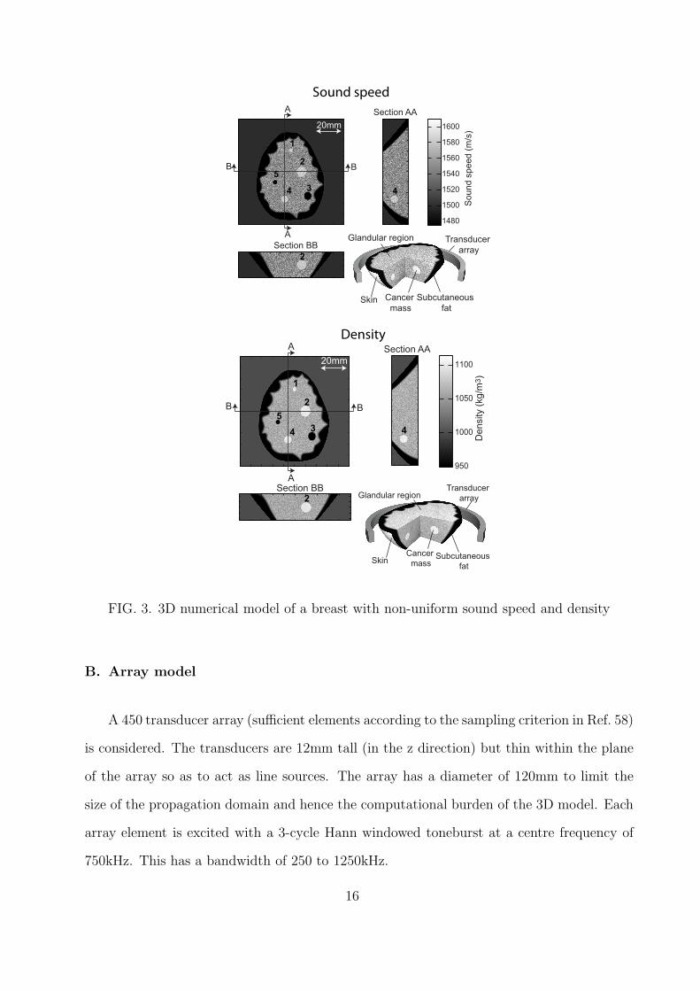
The model is fully 3D to represent the actual shape of the human breast, as shown in

Fig. 3 for the sound speed and density. A glandular region forms the bulk of the breast

model, with an irregular subcutaneous fat layer around the boundary. Material properties

for the glandular region and fat are given in Table I. Existing numerical studies have so far

used data generated by 2D models used to test breast UST algorithms; a novel aspect of

our work is the use of more realistic 3D data for this purpose.

The glandular region is represented by a random medium. As shown in Refs. 55, 56, a

random medium will reduce the amplitude of a transmitted signal by diverting energy away

from the receivers and out of the plane of the array, thus leading to a form of apparent

attenuation. The same effect is produced by the small scale features in the breast which

are also responsible for the speckle phenomenon. We use a random medium model based

on that outlined in Ref. 54, although with longer correlation lengths due to the relatively

large spacing of the FDTD grid. Following the empirical relationship that density tends to

vary linearly with sound speed57, we use the same random field pattern for both density and

velocity.

Five inclusions are placed in the model: three representing cancer masses and two repre-

senting fat spheres. The material properties of these are given in Table I and the dimensions

and locations in Table II. The goal of the imaging algorithm is to be able to detect these

and identify whether each inclusion is cancer from the reconstructed mechanical properties.

15

20mm

1480

1500

1520

1540

1560

1580

1600

Glandular region

Cancer

mass

Subcutaneous

fat

Transducer

array

Skin

A

A

BB

Section AA

Section BB

So

un

d s

pe

ed

(m

/s)

1

4 3

2

5

2

4

A

A

BB

950

1000

1050

110020mm

Section AA

Section BBD

en

sity (

kg

/m3)

4

2

1

4

2

3

5

Glandular region

Cancer

massSubcutaneous

fat

Transducer

array

Skin

Sound speed

Density

FIG. 3. 3D numerical model of a breast with non-uniform sound speed and density

B. Array model

A 450 transducer array (sufficient elements according to the sampling criterion in Ref. 58)

is considered. The transducers are 12mm tall (in the z direction) but thin within the plane

of the array so as to act as line sources. The array has a diameter of 120mm to limit the

size of the propagation domain and hence the computational burden of the 3D model. Each

array element is excited with a 3-cycle Hann windowed toneburst at a centre frequency of

750kHz. This has a bandwidth of 250 to 1250kHz.

16

C. Numerical simulation

A 3D FDTD modelling method is used with a standard Yee grid59, with the mesh

terminated with efficient convolutional perfectly matched layers60 to minimise reflections

from the boundary of the domain. 14 nodes were used per 2mm wavelength, so that the

grid spacing is 1/7 mm. A domain of 861 by 861 by 189 nodes was used. This is large

enough for the 120mm array in the x and y directions and is 24mm tall in the z direction to

allow the beam to diffract as it travels into the domain. A Courant number of 0.95 is chosen

which gives a time step of 2.96×10−8s (based on a maximum velocity of 1620m/s), therefore

needing 4056 time steps for the 0.12ms simulation (long enough for a wave in water to travel

1.5 times the array diameter). The array locations are rounded to the nearest node so the

recorded coordinates for each transducer are adjusted accordingly. 450 separate simulations

have to be performed – one for each illumination. To model the effect of the transducer

out of the plane, each transducer is modelled as a set of in-phase point sources at all nodes

along a 12mm tall line.

A single illumination for this configuration takes around 4 hours to run on a single core

of an AMD Opteron 8384 2.7GHz processor. Parallelism was achieved in a coarse-grained

manner by running many – typically 64 – illuminations simultaneously. Using a cluster of

two quad-core Intel Xeon E5462 2.8GHz processors per node and 40 nodes, running all 450

simulations was completed within around 48 hours, with quite a large dependency on the

queueing system in place on the cluster. These times are for the forward simulation only;

the actual imaging algorithm, running on a single computer, is several orders of magnitude

faster, as detailed in Sec. V.

D. Data Processing

Two sets of data are generated: an incident data set where the material properties

throughout the model are the same as that of water and the set for the case where the breast

phantom described in Sec. IV.A is present. When performing experimental measurements,

17

100 200 300 400

100

200

300

400

-1

0

1

Source Transducer

Re

ce

ive

r T

ran

sd

uce

r

Tim

e (

μs)

Travel times

0.5

-1.5

-0.5

0

0

0

0.002

0.004

0.006

0.008

0.01

0.012

0.014

0.016

Amplitude at 750kHz

100 200 300 400

100

200

300

400

Source Transducer

Re

ce

ive

r T

ran

sd

uce

r

0

0

(a)

(b)

1

1

1

2

1

1

1

2

FIG. 4. Matrices of processed data, plotted for all send-receive pairs. (a) gives the arrival

times of the modelled signals relative to the incident signal, estimated by a frequency domain

deconvolution. (b) presents the amplitude, taken at 750kHz. In both plots, the regions

marked 1 correspond to the transmit-receive pairs with a line-of-sight passing through the

subcutaneous fat layer and those marked 2 to the transducer pairs that ‘see through’ the

volume of the phantom.

the incident data set can be generated by taking measurements when there are no objects

present in the water bath. These data need to be processed prior to passing them through

the imaging algorithms.

Fig. 4(a) presents this difference in arrival times, estimated for all send-receive pairs

18

relative to the incident field. The arrival time is defined as the time at which the first

disturbance is measured at the receiver. These have to be established quantitatively in order

to be able to perform the TFT algorithm; here we use a deconvolution via the frequency

domain. The aim of this deconvolution is to find what the incident signal is convolved with

to generate the total, time-shifted signal; ideally this forms the Dirac delta function, the

offset of which provides the relative time offset. We perform the deconvolution by Fourier

transforming the total signal and dividing by the Fourier transform of the incident signal,

then inverse Fourier transforming the result back to the time domain. The relative arrival

time is taken as the peak of the resulting function. Following the Wiener Deconvolution61 we

add an extra term to the denominator of the division to avoid division by zeros. There are

more accurate methods (e.g. Ref. 62) of establishing the arrival times but this is sufficiently

accurate for us to obtain the low resolution TFT background we need. In the figure, the

regions marked as 2 correspond to the send-receive pairs with a line of sight through the

glandular region of the model; the main effect is to make the waves arrive earlier due to

the higher sound speed of the glandular material. To either side of these diagonal regions,

in the boundaries marked 1, the waves do not pass into the glandular region but only pass

through the subcutaneous fat, which is slower than the water bath and leads to later arrival

of the waves. These therefore appear lighter in the figure.

Fig. 4(b) gives the amplitude of each send-receive pair, produced at 750kHz by taking a

discrete Fourier transform of the measured data. The data have been normalised such that

they represent what would be seen if a unit point source was used to provide the illumination.

If there was no scatterer present then the field would be the same as the Green’s function

sampled around the array. Under this condition, a singularity would be present along the

principal diagonal due to the measurement being taken at the source location. However,

this singularity is removed by gating off the incident signal for the source and surrounding

measurements, which leaves the dark stripe down the diagonal.

The bright boundaries (marked 1) are the waves which have passed solely through the

subcutaneous fat. The relatively high amplitude indicates that some form of focusing is

19

occurring. Waves passing through the bulk of the glandular region, 2, have lower amplitude

due to the effects of the random glandular material that scatters sound in all directions in

space. The diagonal crossing patterns throughout this region are due to the presence of the

inclusions.

V. RESULTS

Fig. 5 shows the separate stages of HARBUT compared to the original sound speed

model of the central slice of the phantom in Fig. 5(a). The TFT reconstruction in Fig. 5(b)

shows the expected low resolution characteristics since diffraction is not accounted for. The

reconstruction allows us to detect the subcutaneous fat layer and the glandular region;

however, the inclusions are not reliably detectable. Enhanced TFT reconstructions are

likely to be possible – for example by using a higher centre frequency to improve resolution

– but the improvements will still be fundamentally limited by the algorithm’s inability to

deal with diffraction.

Fig. 5(c) is the modified BF image using the background from Fig. 5(b). The absolute

value of the complex values at each pixel is plotted. In this reconstruction, the total field

ψ is used rather than the perturbation ψδ. The features are masked by the presence of

the transmission signals in the data used to reconstruct the image. Converting to the DT

image in Fig. 5(d), using the filter from Ref. 43 based on the free space kw, allows all

five inclusions to be identified. The inclusions appear inverted because of the definition of

the object function in eq. (3). This perturbation component is sufficiently small that the

approximation ψ = ψb necessary for the algorithm to work is valid. The total object function

in Fig. 5(e) is calculated by combining Ob from Fig. 5(b) and the Oδ in Fig. 5(d) according

to (5).

Fig. 5(f) is the final sound speed reconstruction obtained from Fig. 5(e) by inverting (3)

and ignoring density effects. All five inclusions can be very clearly seen and all the irregular

features of the subcutaneous fat layer are reconstructed. The sharp boundaries at the edge

20

1480

1500

1520

1540

1560

1580

1600

So

un

d s

pe

ed

(m

/s)

20mm

(a)

(b)TFT reconstructionOriginal central slice

(c)Corrected BF image

(d)

Hybrid velocity reconstruction(e)

Oδ component of hybrid image

(f)

Array

Hybrid reconstruction of O

1480

1500

1520

1540

1560

1580

1600

So

un

d s

pe

ed

(m

/s)

No

n-d

ime

nsio

na

l

1480

1500

1520

1540

1560

1580

1600

So

un

d s

pe

ed

(m

/s)

−106

106

0

m-2

1

0

2

3

4

5

6

7

8

x10-4

−106

106

0

m-2

FIG. 5. (a) The original central slice of the sound speed map as in Fig. 3, with the locations

of the transducer array marked. (b) is the TFT sound speed reconstruction. This is used

as the background for the corrected beamforming at 750kHz in (c). The modulus of the

complex reconstruction is given. This is then filtered to get the object function perturbation

component Oδ given in (d). (e) is the full object function O generated by combining (d)

and the background object function Ob calculated from (b). (f) is the hybrid sound speed

reconstruction from the object function (e).

21

1480

1500

1520

1540

1560

1580

1600

So

un

d s

pe

ed

(m

/s)

20mm

(a)Original central slice (b)DT reconstruction

FIG. 6. Standard DT reconstruction. The size and the contrast of the original phantom (a)

are large enough that the standard Born approximation is invalid, causing the reconstruction

(b) to have extensive artefacts that obscure the inclusions.

of the model and at the edge of the glandular region are blurred in the reconstruction; also

the random medium representing the glandular region appears more homogeneous. This

blurring is due to an averaging effect in the z direction that determines the so called slice

thickness63 as discussed in Sec. VI. This effect is also responsible for the reconstructed

contrast of inclusion 1 being reduced.

In Tab. III we present the average sound speeds through each of the reconstructed

inclusions. Due to the z-direction averaging, the contrast tends to be reduced, particularly

for the smaller inclusions. Overall, however, all inclusions are reconstructed with a small

error – within 0.72% – and the image is a dramatic improvement over the TFT reconstruction

of Fig. 5(b).

The use of beamforming before the application of the DT filter makes HARBUT very

robust against noise. We have tested how HARBUT performs when noise is present by

adding a noise matrix, N, to the matrix in Fig. 4(b). The entries of the N-matrix are

complex random numbers with a Gaussian amplitude distribution with standard deviation

s and phase uniformly distributed between −π and π. The noise level is defined as the ratio

between s and the rms value of the moduli of the entries in the matrix in Fig. 4(b). The

sound speed reconstruction with the noise present has a slightly granular appearance, but

apart from this is effectively unchanged.

Finally, to demonstrate the effectiveness of HARBUT, Fig. 6(b) shows the reconstruction

22

obtained with the standard BF/DT algorithm43 with a homogeneous water background. Due

to the size and contrast of the phantom relative to the water background, the condition for

validity of the Born approximation is violated. As the illuminating field travels inside the

phantom, it accumulates a phase delay larger than π. As a result, the total field that

propagetes through the object is in opposition of phase with the free space incident field

(which replaces it under the Born approximation) leading to the artefacts in Fig. 6(b).

The current implementation of the BF/DT stage uses Matlab. To generate the 481 by

481 pixel image given the background correction data currently takes around 60 seconds on

an HP z600 dual quad-core workstation without significant optimisation. The background

correction data, required to calculate Gb, are taken from the final iteration of the TFT

algorithm and therefore have no associated overhead. We have also produced an optimised

C++ version which produces the same image in 5 seconds. This compares to the TFT

method itself which takes around 1 minute to complete (although this is strongly dependent

on parameters such as pixel size) and DBIM which according to one example, where it is

applied to breast ultrasound tomography50, took around 9 hours per iteration for a relatively

small domain of 50λ by 50λ.

VI. PRACTICAL CONSIDERATIONS

In this section we discuss the practical aspects that were introduced at the end of Sec. III,

points 1) to 4).

A. 3D effects and sampling conditions

Fig. 7 compares the hybrid image from the 3D data as in Fig. 5(f) with a reconstruction

using data from a similar simulation, except performed in 2D using the central slice of

Fig. 3. The 2D reconstruction has sharp boundaries at the edge of the glandular region

and the breast itself, which are both blurred in the 3D version. The granular appearance

of the random medium is also better defined in the 2D reconstruction than the 3D. These

23

1480

1500

1520

1540

1560

1580

1600

So

un

d s

pe

ed

(m

/s)

3D data 2D data

20mm

(a) (b)

FIG. 7. Comparison of the HARBUT reconstruction from 3D data (a) and 2D data (b).

The boundaries of the glandular region and the phantom itself in the 3D reconstruction are

blurred in comparison to the 2D reconstruction. The random medium which makes up the

glandular region is also more homogeneous in the 3D reconstruction. These effects are a

result of averaging in the out-of-plane direction.

differences are caused by blurring in the z (out-of-plane) direction in the 3D reconstruction

due to the finite height of the transducer beam, as will be explained in this section.

For this purpose it is necessary to consider the 3D Point Spread Function (PSF) which

gives the response of the imaging system to a point scatterer. If the PSF is space invariant,

i.e. does not depend on the position of the point scatterer, then the image is a convolution

of the PSF with the original object function. The PSF is space invariant for standard DT43,

assuming plane wave illuminations and measurements taken in the far field, and here we

assume that it can also be considered space invariant for HARBUT due to the relatively low

contrast of the background sound speed map.

To generate the 3D PSF, a point scatterer at the origin – the centre of the array at z = 0

– is imaged with the transducer array at several axial locations; these images are then stacked

to form the point scatterer response. Fig. 8 gives the PSF for the system considered in this

paper. In the x and y directions it is 1mm (λ/2) thick because of the Born approximation

resolution limit, but in the z direction – as shown in Fig. 8(d) – the response stretches out

to around ±4.5mm, using a threshold of −6dB relative to the maximum.

Due to the convolution, each point in the final image will be a weighted average of the

object function in the z direction with the weights defined by the PSF projection in Fig. 8.

24

x

y

z

0

1

x

z

x

y

-6dB threshold

-10

10

0

z (

mm

)y (

mm

)

0

-5

5

(a)(b)

(c)

(d)

(e)

4.5

FIG. 8. Normalised Point Spread Function at the centre of the array for the system modelled

in this paper – 12mm tall transducers with an array diameter of 120mm. The PSF is thin –

about 1mm (λ/2) wide – within the plane due to the resolution of the Born approximation

used in the reconstruction. As shown in (d), taking a threshold at −6dB relative to the

maximum, the PSF extends in the region −4.5mm< z < 4.5mm, making its height around

9mm. This is significantly wider than the in-plane PSF dimensions.

This means that any structure not aligned in the z direction will be blurred in the final

reconstruction. This is evident in Fig. 5(f), where the boundaries of the glandular region

and the subcutaneous fat layer becomed blurred since they intersect the imaging plane at

an oblique angle.

The extent of the interval in the z direction over which material properties are averaged

defines the slice thickness. To estimate the slice thickness, a simple ‘spiral staircase’ model

is used. This consists of point scatterers at a series of heights and a series of radii, with the

points at each particular height being arranged in one radial direction, forming the steps in

the staircase. Fig. 9(a) shows this schematically.

The scatterers are placed at heights of 0-10mm with 0.5mm gaps and radii of 15-50mm

with 5mm gaps. Fig. 9(b) is the image obtained with the hybrid method at one position of the

array. For an ideal imaging system with 0mm slice thickness the image should contain only

a single set of eight scatterers along the radial direction in the plane at z = 0. Instead, due

25

0

1

z = 0mm

1mm

2mm3mm

4mm

5mm

6mm

7mm 8mm

9mm

10mm

Normalised magnitude of

reconstructed object function

-6dB

drop

‘Staircase’

continues

x

z

y

Transducer array

(a) (b)

FIG. 9. (a) is a schematic 3D diagram of the arrangement of scatterers in the spiral staircase

model. (b) gives the 2D reconstruction of data from such a model, simulated with the 3D

FDTD method, for heights 0-10mm at 0.5mm gaps and radii of 15-50mm at 5mm gaps.

The artefacts surrounding each scatterer are a result of the relatively course FDTD mesh

used, rather than the imaging process, and are ignored. The transducers are modelled as

the 12mm tall line sources used in all the simulations in this paper and are at a radius of

60mm. There is a clear drop in response as the height of the scatterer is increased due to the

transducer beam height. Following Fig. 8(d), the 4.5mm z offset points lie around the −6dB

threshold, indicating this is the boundary of the slice captured by the transducer array.

to the spreading of the PSF in the z direction, weaker reconstructions of the scatterers from

different heights can be observed. However, the amplitude of the reconstructed scatterers

decays as the corresponding distance from the plane of the array increases. In particular a

−6dB drop in amplitude can be observed for the scatterers at z = 4.5mm, thus verifying

that the slice thickness is around 9mm.

The finite slice thickness is a result of the reduction in sensitivity of the transducer

array to scatterers at greater distances from z = 0. The sensitivity of the array drops

because there is a reduction in both 1) the amplitude of the illuminating beam incident on

the scatterer and 2) the sensitivity of the receiving transducer to waves from the scatterer.

Here, we consider only a point scatterer along the axis of the array so that the distances to

all transducers are the same, and therefore, by the principle of reciprocity, 1) and 2) will

both cause the same amplitude drop. Therefore, the −6dB drop in array sensitivity, which

26

defines the boundary of the slice thickness, will be achieved when the illuminating beam

and the receiver sensitivity each drop by −3dB. Considering the Fraunhofer zone of a line

transducer64, the thickness of the beam, B, at the centre of the array with a −3dB threshold

as

B =0.884λrarr

h(18)

where rarr is the radius of the array and h is the transducer height. For the case considered

here, the −6dB slice thickness becomes 8.8mm at the centre of the array, which is close

enough to the 9mm slice thickness to verify the validity of (18). Equation (18) shows

that it is possible that the slice thickness could be reduced by increasing the height of the

transducers, although the benefit of this is limited because the Fraunhofer approximation

becomes invalid with large transducers. Alternatively, a synthetic aperture approach could

be used to reduce the slice thickness as described in Ref. 65.

B. The subtraction problem

The beamforming algorithm in (16) uses the field ψδ, which is calculated as the difference

between the measured field and the background field

ψδ = ψ − ψb. (19)

However, to obtain the reconstructions in Fig. 5 we have used the total field ψ that is directly

available from the measurements in place of ψδ. Here, we justify why this is possible.

In principle, ψb could be calculated by solving the wave equation with the background

field with the FDTD method. However, this would not be reliable in practice because the

perturbation field ψδ is small compared to ψ and ψb, so any small errors in the estimation of

ψb will cause large errors in ψδ. Errors in the ψb estimation are unavoidable, mainly because

of uncertainty in the transducer response.

Here, we show that it is not necessary to perform the subtraction and it is sufficient to

27

1480

1500

1520

1540

1560

1580

1600

−0.06 −0.04 −0.02 0 0.02 0.04 0.061494

1496

1498

1500

1502Sound speed reconstruction Sound speed along y = 0

(a) (b)

y = 0

x position (m)

So

un

d s

pe

ed

(m

/s)

20mm

FIG. 10. Image generated by imaging ψδ = ψb in the corresponding background velocity

field. This is present in the final image if the subtraction is not performed. The error is

within ±1m/s through the majority of the imaging domain.

form the BF image from the measured total field directly, i.e.

Iδ (z) =

∫

ψ

GbGb

dx′. (20)

For this purpose it is observed that the BF and filtering steps in HARBUT are linear (for

a fixed background) with respect to the measurements. This means that we can define a

linear operator, IDT , that maps the measurements or data, d, onto an image, i, i.e.

i = IDT (d) . (21)

When the data correspond to ψδ then Oδ = IDT (ψδ). If instead, the data correspond to the

total field then

IDT (ψ) = IDT (ψδ) + IDT (ψb) = Oδ + IDT (ψb) . (22)

The term IDT (ψb) therefore represents the error caused by making the assumption that the

background field does not need to be subtracted. Fig. 10 shows IDT (ψb) converted to a

velocity image for the ψb calculated for the TFT background of Fig. 5(b). The velocity map

is within ±1m/s of the background except the region outside the array where ring artefacts

appear, which is an acceptably small error given that the structures of interest to us have a

sound speed contrast relative to the background in the order of 5%.

This convenient property makes the proposed approach very robust because it means

that we do not need to estimate ψb, thus avoiding significant sources of error.

28

1480

1500

1520

1540

1560

1580

160020mm

So

un

d s

pe

ed

(m

/s)

FIG. 11. The artefacts caused by ignoring density variations in the velocity reconstructions.

This image is produced from a new 2D simulation. This simulation uses a constant sound

speed field of 1500m/s and a density field corresponding to the central slice from Fig. 3.

The reconstruction, as with the rest of the paper, assumes density to be negligible and

reconstructs the resulting field as velocity perturbations.

C. Density

Here we show that density variations within the breast can be neglected.

Equation (3) defines the object function, which includes a term dependent on the density

field. The form of this term means that in order for the density to contribute a significant

amount to O (r), a large density gradient must be present. Within soft tissue, density varies

continuously; therefore the object function, O, is mainly defined by the sound speed. Even

if the density were to vary suddenly at the interface of a cancer mass, the limited density

contrast would still make the density term in (3) negligible.

It is possible to isolate the effects of the density field from the velocity field in the

reconstruction by performing a new forward simulation with only the density variations

present and a constant sound speed. We have performed this simulation in 2D using the

central slice from Fig. 3 for the density field. The reconstruction with this data is given

in Fig. 11. The sound speed map is obtained assuming that the density term in (3) is

negligible. If this were true the reconstructed velocity should be 1500m/s (the same as

29

the water background) across the image plane, but instead different values of sound speed

are seen where density discontinuities occur, showing that density affects the sound speed

reconstruction to some extent. However, the values of sound speed significantly differ from

the background velocity only at the boundaries of sudden density variations. This leads to

two main conclusions: 1) the absolute value of density does not affect the velocity estimate; 2)

the errors in velocity at sudden density variations help the visualisation of these boundaries

and therefore aid the definition of complex morphologies. It is recognised, however, that

density could subsequently be determined from the image by using multiple frequencies

according to the approach outlined in Ref. 66.

D. Amplitude correction

The amplitudes of the waves drop as they pass through the 3D breast phantom. One

cause of this is the random medium of the glandular region, which scatters energy from the

waves in all directions. Some of the energy is scattered out of the plane of the array and is

lost; 2D reconstructions ignore this so it becomes a form of attenuation. A second amplitude

loss occurs due to the oblique angle at which the wave hits the phantom boundary. The wave

is refracted slightly upwards (or downwards depending on the relative sound speeds of the

breast and the water) which causes an amplitude drop due to the misalignment of the wave

with the receiver67. In experimental data both these effects will be present, along with the

attenuation caused by the material itself. This loss in amplitude, if it is not accounted for,

will cause the reconstructed object function perturbation Oδ to be too small. However, one

solution to this problem would be to correct the amplitude loss in the same way we correct

the phase. A ray-based attenuation image could be formed in the manner of the TFT image,

which would include material attenuation, as well as 3D scattering and deflection since the

effects are inseparable. From this, the wave amplitudes at all points in the domain for

all illuminations could be calculated using a forward model, which could then correct the

Green’s functions used in the BF algorithm.

30

0 50 100 150 200 250 300 350 400 4500

1

Transducer

Source Through transmission

Ave

rag

ed

re

lative

sig

na

l a

mp

litu

de

0.1

0.2

0.3

0.4

0.5

0.6

0.7

0.8

0.9

Ratio

approximated

to 0.5

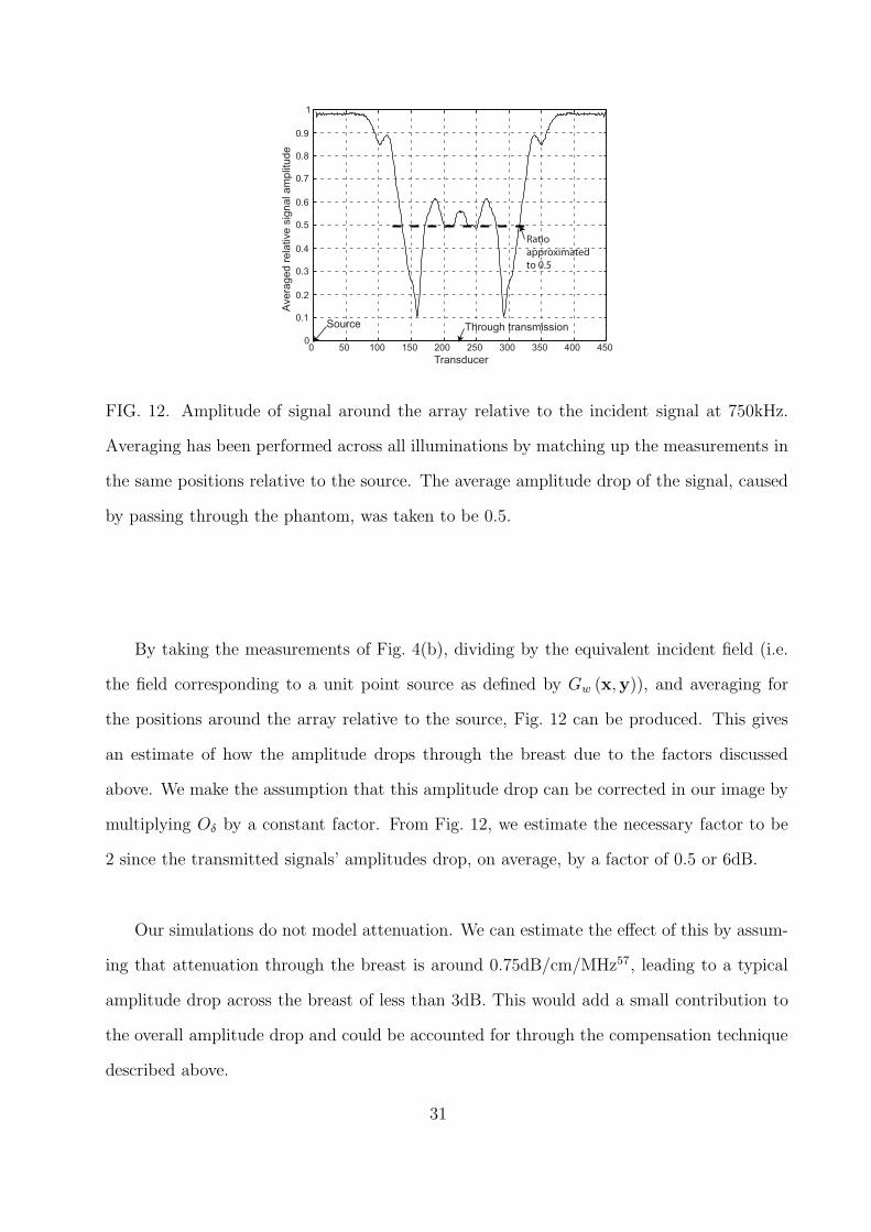
FIG. 12. Amplitude of signal around the array relative to the incident signal at 750kHz.

Averaging has been performed across all illuminations by matching up the measurements in

the same positions relative to the source. The average amplitude drop of the signal, caused

by passing through the phantom, was taken to be 0.5.

By taking the measurements of Fig. 4(b), dividing by the equivalent incident field (i.e.

the field corresponding to a unit point source as defined by Gw (x,y)), and averaging for

the positions around the array relative to the source, Fig. 12 can be produced. This gives

an estimate of how the amplitude drops through the breast due to the factors discussed

above. We make the assumption that this amplitude drop can be corrected in our image by

multiplying Oδ by a constant factor. From Fig. 12, we estimate the necessary factor to be

2 since the transmitted signals’ amplitudes drop, on average, by a factor of 0.5 or 6dB.

Our simulations do not model attenuation. We can estimate the effect of this by assum-

ing that attenuation through the breast is around 0.75dB/cm/MHz57, leading to a typical

amplitude drop across the breast of less than 3dB. This would add a small contribution to

the overall amplitude drop and could be accounted for through the compensation technique

described above.

31

VII. CONCLUSIONS

We have introduced HARBUT, the Hybrid Algorithm for Robust Breast Ultrasound To-

mography, which provides a resolution improvement over Time-of-Flight Tomography while

avoiding the convergence and speed problems of iterative methods. Diffraction Tomography

methods are unsuitable for this purpose because the contrast and size of the breast relative

to the homogeneous water background breaks the Born approximation. By reformulating

the problem using an inhomogeneous background which is sufficiently close to the actual

sound speed map, the relative contrast can be reduced such that the approximation becomes

valid.

It is shown that the TFT algorithm can provide such a background. Imaging against

this is performed in two stages. A modified BF algorithm, using Green’s functions calculated

for the background, generates the first image. This is then converted into the equivalent DT

image by filtering in the spatial frequency domain.

HARBUT is demonstrated to accurately reconstruct the sound speed through a breast

phantom model from 3D simulated data, despite sampling the wavefield with an array ar-

chitecture suitable for 2D imaging, and the presence of uncertainties such as transducer

response that are likely to occur in real experiments. At a frequency of 750kHz, masses

as small as 4mm in diameter can be clearly imaged. An in-plane resolution of 1mm was

achieved, with a slice thickness of 9mm. Density contrast and randomly varying material

properties with sub-wavelength coherence lengths have little influence on the final recon-

struction. 3D structures intersecting the plane of the array are partially projected onto the

imaging plane due to the size of the slice thickness.

Acknowledgments

The authors would like to thank EPSRC for supporting this research with grant

EP/F00947X/1.

32

References

1 F. Kamangar, G. Dores, and W. Anderson, “Patterns of cancer incidence, mortality,

and prevalence across five continents: defining priorities to reduce cancer disparities in

different geographic regions of the world”, Journal of Clinical Oncology 24, 2137 (2006).

2 P. Autier, M. Boniol, C. LaVecchia, L. Vatten, A. Gavin, C. Hery, and M. Heanue, “Dis-

parities in breast cancer mortality trends between 30 european countries: retrospective

trend analysis of who mortality database”, British Medical Journal 341, 3620 (2010).

3 M. Silverstein, M. Lagios, A. Recht, D. Allred, S. Harms, R. Holland, D. Holmes,

L. Hughes, R. Jackman, T. Julian, et al., “Image-detected breast cancer: state of the

art diagnosis and treatment”, Journal of the American College of Surgeons 201, 586–597

(2005).

4 T. M. Kolb, J. Lichy, and J. H. Newhouse, “Comparison of the performance of screening

mammography, physical examination, and breast us and evaluation of factors that influ-

ence them: An analysis of 27,825 patient evaluation”, Radiology 225, 165–175 (2002).

5 P. C. Stomper, D. J. D’Souza, P. A. Dinitto, and et al., “Analysis of parenchymal density

on mammograms in 1353 women 25-79 years old”, AJR Am J Roentgenol 167, 1261–1265

(1996).

6 D. Saslow, C. Boetes, W. Burke, S. Harms, M. Leach, C. Lehman, E. Morris, E. Pisano,

M. Schnall, S. Sener, et al., “American cancer society guidelines for breast screening with

mri as an adjunct to mammography”, CA: A Cancer Journal for Clinicians 57, 75 (2007).

7 M. Kriege, C. Brekelmans, C. Boetes, P. Besnard, H. Zonderland, I. Obdeijn, R. Manoliu,

T. Kok, H. Peterse, M. Tilanus-Linthorst, et al., “Efficacy of mri and mammography for

breast-cancer screening in women with a familial or genetic predisposition”, The New

England journal of medicine 351, 427 (2004).

8 J. F. Greenleaf, S. A. Johnson, S. L. Lee, G. T. Herman, and E. H. Wood, “Algebraic

reconstruction of spatial distributions of acoustic absorption within tissue from their two-

dimensional acoustic projections”, International Symposium on Acoustical Holography

33

and Imaging, 5th, Palo Alto, Calif 5, 591–603 (1973).

9 P. Carson, C. Meyer, A. Scherzinger, and T. Oughton, “Breast imaging in coronal planes

with simultaneous pulse echo and transmission ultrasound”, Science 214, 1141 (1981).

10 J. Schreiman, J. Gisvold, J. Greenleaf, and R. Bahn, “Ultrasound transmission computed

tomography of the breast”, Radiology 150, 523 (1984).

11 M. P. Andre, H. S. Janee, P. Martin, G. P. Otto, B. A. Spivey, and D. A. Palmer, “High-

speed data acquisition in a diffraction tomography system employing large-scale toroidal

arrays”, Int. J. Imag. Syst. Tech. 8, 137–147 (1997).

12 N. Duric, P. Littrup, L. Poulo, A. Babkin, R. Pevzner, E. Holsapple, O. Rama, and

C. Glide, “Detection of breast cancer with ultrasound tomography: First results with the

computed ultrasound risk evaluation (cure) prototype”, Medical physics 34, 773 (2007).

13 H. Gemmeke and N. Ruiter, “3d ultrasound computer tomography for medical imag-

ing”, Nuclear Instruments and Methods in Physics Research Section A: Accelerators,

Spectrometers, Detectors and Associated Equipment 580, 1057–1065 (2007).

14 S. Mensah and E. Franceschini, “Near-field ultrasound tomography”, J. Acoust. Soc. Am.

121, 1423–33 (2007).

15 C. Hansen, N. Huttebrauker, H. Ermert, M. Hollenhorst, L. Heuser, and G. Schulte-

Altedorneburg, “Determination of a mean sound velocity in the female breast for artifact

reduction in full angle spatial compounding”, in Ultrasonics Symposium (IUS), 2009

IEEE International, 538–541 (IEEE) (2010).

16 J. F. Greenleaf, S. A. Johnson, W. F. Samayoa, and F. A. Duck, “Algebraic reconstruction

of spatial distributions of acoustic velocities in tissue from their time-of-flight profiles”,

in Acoustical Holography, edited by P. S. Green, volume 6, 71–90 (Plenum Press, New

York) (1975).

17 J. Greenleaf, S. Johnson, and R. Bahn, “Quantitative cross-sectional imaging of ultra-

sound parameters”, in Ultrasonics Symposium, 1977, 989–995 (1977).

18 H. Schomberg, “An improved approach to reconstructive ultrasound tomography”, Jour-

nal of Physics D: Applied Physics 11, L181 (1978).

34

19 M. Krueger, A. Pesavento, and H. Ermert, “A modified time-of-flight tomography concept

for ultrasonic breast imaging”, IEE Ultrasonics Symposium 1381–1385 (1996).

20 Y. Quan and L. Huang, “Sound-speed tomography using first-arrival transmission ultra-

sound for a ring array”, in Proc. SPIE, volume 6513, pp. 651306-1–651306-9 (2007).

21 S. Li, M. Jackowski, D. Dione, T. Varslot, L. Staib, and K. Mueller, “Refraction corrected

transmission ultrasound computed tomography for application in breast imaging”, Med-

ical Physics 37, 2233 (2010).

22 A. Hormati, I. Jovanovic, O. Roy, and M. Vetterli, “Robust ultrasound travel-time tomog-

raphy using the bent ray model”, in Society of Photo-Optical Instrumentation Engineers

(SPIE) Conference Series, volume 7629, pp. 76290I-1–76290I-12 (2010).

23 K. Tanabe, “Projection method for solving a singular system of linear equations and its

applications”, Numerische Mathematik 17, 203–214 (1971).

24 A. Louis and F. Natterer, “Mathematical problems of computerized tomography”, Pro-

ceedings of the IEEE 71, 379–389 (1983).

25 P. Williamson, “A guide to the limits of resolution imposed by scattering in ray tomog-

raphy”, Geophysics 56, 202–207 (1991).

26 R. Snieder and A. Lomax, “Wavefield smoothing and the effect of rough velocity perturba-

tions on arrival times and amplitudes”, Geophysical Journal International 125, 796–812

(1996).

27 G. Schuster, “Resolution limits for crosswell migration and traveltime tomography”, Geo-

physical Journal International 127, 427–440 (1996).

28 R. Pratt, “Seismic waveform inversion in the frequency domain, part 1: Theory and

verification in a physical scale model”, Geophysics 64, 888–901 (1999).

29 P. Thore and C. Juliard, “Fresnel zone effect on seismic velocity resolution”, Geophysics

64, 593–603 (1999).

30 S. Hung, F. Dahlen, and G. Nolet, “Wavefront healing: a banana–doughnut perspective”,

Geophysical Journal International 146, 289–312 (2001).

31 J. Spetzler, C. Sivaji, O. Nishizawa, and Y. Fukushima, “A test of ray theory and scat-

35

tering theory based on a laboratory experiment using ultrasonic waves and numerical

simulation by finite-difference method”, Geophysical Journal International 148, 165–178

(2002).

32 A. Devaney, “A filtered backpropagation algorithm for diffraction tomography”, Ultra-

sonic imaging 4, 336–350 (1982).

33 M. Born and E. Wolf, Principles of Optics pp. 695–703 (Cambridge University Press,

Cambridge) (1999).

34 A. C. Kak and M. Slaney, Principles of computerized tomographic reconstruction pp.

203–218 (IEEE Press, New York) (1998).

35 F. Simonetti, L. Huang, N. Duric, and P. Littrup, “Diffraction and coherence in breast

ultrasound tomography: A study with a toroidal array”, Medical physics 36, 2955 (2009).

36 F. Natterer and F. Wubbeling, Mathematical methods in image reconstruction pp. 1–216

(Society for Industrial Mathematics) (2001).

37 A. Tarantola, Inverse problem theory and methods for model parameter estimation pp.

1–630(Society for Industrial Mathematics) (2005).

38 J. Wiskin, D. Borup, S. Johnson, M. Berggren, T. Abbott, and R. Hanover, “Full-wave,

non-linear, inverse scattering”, Acoustical Imaging 183–193 (2007).

39 T. D. Mast, “Aberration correction for time-domain ultrasound diffraction tomography”,

The Journal of the Acoustical Society of America 112, 55 (2002).

40 P. M. Morse and K. U. Ingard, Theoretical Acoustics, pp. 227–305 (McGraw-Hill Book

Company, New York, London) (1968).

41 S. Pourjavid and O. Tretiak, “Numerical solution of the direct scattering problem through

the transformed acoustical wave equation”, The Journal of the Acoustical Society of

America 91, 639 (1992).

42 W. Chew and Y. Wang, “Reconstruction of two-dimensional permittivity distribution

using the distorted born iterative method”, IEEE Transactions on Medical Imaging 9,

218–225 (1990).

43 F. Simonetti and L. Huang, “From beamforming to diffraction tomography”, Journal of

36

Applied Physics 103, 103110 (2008).

44 S. Norton and M. Linzer, “Ultrasonic reflectivity imaging in three dimensions: exact

inverse scattering solutions for plane, cylindrical, and spherical apertures.”, IEEE trans-

actions on bio-medical engineering 28, 202 (1981).

45 F. Anderson and F. Morgan, “Active imaging analysis via ellipsoidal projections”, Acous-

tical imaging 21, 171–182 (1995).

46 J. Jensen, S. Nikolov, K. Gammelmark, and M. Pedersen, “Synthetic aperture ultrasound

imaging”, Ultrasonics 44, e5–e15 (2006).

47 S. Li, K. Mueller, M. Jackowski, D. Dione, and L. Staib, “Fast marching method to

correct for refraction in ultrasound computed tomography”, in 3rd IEEE International

Symposium on Biomedical Imaging: Nano to Macro, 2006, 896–899 (2006).

48 J. Sethian, “A fast marching level set method for monotonically advancing fronts”, Pro-

ceedings of the National Academy of Sciences of the United States of America 93, 1591

(1996).

49 W. Schneider, “Integral formulation for migration in two and three dimensions”, Geo-

physics 43, 49 (1978).

50 M. Haynes and M. Moghaddam, “Large-domain, low-contrast acoustic inverse scattering

for ultrasound breast imaging”, Biomedical Engineering, IEEE Transactions on 57, 2712–

2722 (2010).

51 T. D. Mast, “Wideband quantitative ultrasonic imaging by time-domain diffraction to-

mography”, The Journal of the Acoustical Society of America 106, 3061 (1999).

52 C. Li, N. Duric, P. Littrup, and L. Huang, “In vivo breast sound-speed imaging with

ultrasound tomography”, Ultrasound in medicine & biology 35, 1615–1628 (2009).

53 S. Goss, R. Johnston, and F. Dunn, “Comprehensive compilation of empirical ultrasonic

properties of mammalian tissues”, The Journal of the Acoustical Society of America 64,

423 (1978).

54 E. Franceschini, S. Mensah, D. Amy, and J. Lefebvre, “A 2-d anatomic breast ductal com-

puter phantom for ultrasonic imaging”, IEEE transactions on ultrasonics, ferroelectrics,

37

and frequency control 53, 1281 (2006).

55 L. Foldy, “The multiple scattering of waves. i. general theory of isotropic scattering by

randomly distributed scatterers”, Physical Review 67, 107–119 (1945).

56 M. Cowan, K. Beaty, J. Page, Z. Liu, and P. Sheng, “Group velocity of acoustic waves

in strongly scattering media: Dependence on the volume fraction of scatterers”, Physical

Review E 58, 6626–6636 (1998).

57 T. D. Mast, “Empirical relationships between acoustic parameters in human soft tissues”,

Acoustics Research Letters Online 1, 37 (2000).

58 F. Simonetti, L. Huang, and N. Duric, “On the sampling of the far-field operator with a

circular ring array”, J. Appl. Phys. 101, 083103 (2007).

59 K. Yee, “Numerical solution of inital boundary value problems involving maxwell’s equa-

tions in isotropic media”, IEEE Transactions on antennas and propagation 14, 302–307

(1966).

60 D. Komatitsch and R. Martin, “An unsplit convolutional perfectly matched layer im-

proved at grazing incidence for the seismic wave equation”, Geophysics 72, 155–167

(2007).

61 N. Wiener, Extrapolation, interpolation, and smoothing of stationary time series pp. 1–

116 (The MIT Press) (1964).

62 C. Li, L. Huang, N. Duric, H. Zhang, and C. Rowe, “An improved automatic time-of-flight

picker for medical ultrasound tomography”, Ultrasonics 49, 61–72 (2009).

63 A. Goldstein and B. Madrazo, “Slice-thickness artifacts in gray-scale ultrasound”, Journal

of Clinical Ultrasound 9, 365–375 (1981).

64 J. W. Goodman, Introduction to Fourier Optics pp. 73–75 (McGraw-Hill, New York)

(1996).

65 F. Simonetti and L. Huang, “Synthetic aperture diffraction tomography for three-

dimensional imaging”, Proceedings of the Royal Society A: Mathematical, Physical and

Engineering Science 465, 2877 (2009).

66 R. Lavarello and M. Oelze, “Density imaging using inverse scattering”, The Journal of

38

the Acoustical Society of America 125, 793 (2009).

67 F. Simonetti, L. Huang, and N. Duric, “A multiscale approach to diffraction tomography

of complex three-dimensional objects”, Appl. Phys. Lett. 95, 061904 (2009).

39

TABLE I. Material properties of the structures in the breast phantom

Structure Sound speed (m/s) Density (kg/m3) Standard deviation (%) Correlation length (mm)

Water 1500 1000 - -

Glandular region 1550 1060 2 1.5

Fat 1470 950 - -

Cancer masses 1580 1100 1 1.5

40

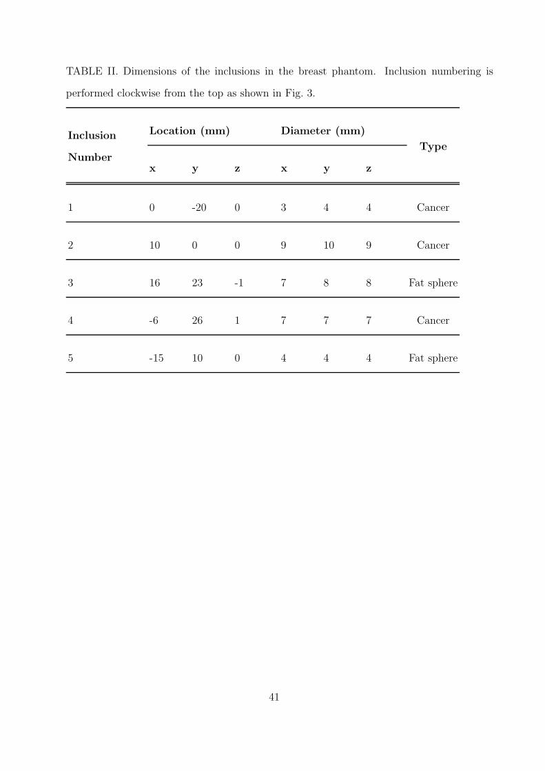
TABLE II. Dimensions of the inclusions in the breast phantom. Inclusion numbering is

performed clockwise from the top as shown in Fig. 3.

Inclusion

Number

Location (mm) Diameter (mm)

Type

x y z x y z

1 0 -20 0 3 4 4 Cancer

2 10 0 0 9 10 9 Cancer

3 16 23 -1 7 8 8 Fat sphere

4 -6 26 1 7 7 7 Cancer

5 -15 10 0 4 4 4 Fat sphere

41

TABLE III. Reconstructed average sound speeds within each inclusion

Inclusion Actual sound speed (m/s) Reconstructed sound speed (m/s) Error

1 1580 1568 0.76%

2 1580 1575 0.32%

3 1470 1463 0.48%

4 1580 1571 0.57%

5 1470 1473 0.20%

42

List of Figures

FIG. 1 Schematic of the system for breast ultrasound tomography. (a) The patient

lies prone with the breast suspended in a water tank. A transducer array

begins at the chest wall and gathers sets of data at many slices through the

breast. Shown in (b) is a single illumination and the scattered field produced

which is measured by the transducer array. We define x′ as a point inside

the scatterer. . . . . . . . . . . . . . . . . . . . . . . . . . . . . . . . . . . . 4

FIG. 2 Flowchart of the stages which make up the original BF/DT algorithm, and

the additional TFT stage which is included in HARBUT . . . . . . . . . . . 11

FIG. 3 3D numerical model of a breast with non-uniform sound speed and density . 16

FIG. 4 Matrices of processed data, plotted for all send-receive pairs. (a) gives the

arrival times of the modelled signals relative to the incident signal, estimated

by a frequency domain deconvolution. (b) presents the amplitude, taken at

750kHz. In both plots, the regions marked 1 correspond to the transmit-

receive pairs with a line-of-sight passing through the subcutaneous fat layer

and those marked 2 to the transducer pairs that ‘see through’ the volume of

the phantom. . . . . . . . . . . . . . . . . . . . . . . . . . . . . . . . . . . . 18

FIG. 5 (a) The original central slice of the sound speed map as in Fig. 3, with

the locations of the transducer array marked. (b) is the TFT sound speed

reconstruction. This is used as the background for the corrected beamforming

at 750kHz in (c). The modulus of the complex reconstruction is given. This

is then filtered to get the object function perturbation component Oδ given

in (d). (e) is the full object function O generated by combining (d) and the

background object function Ob calculated from (b). (f) is the hybrid sound

speed reconstruction from the object function (e). . . . . . . . . . . . . . . . 21

43

FIG. 6 Standard DT reconstruction. The size and the contrast of the original phan-

tom (a) are large enough that the standard Born approximation is invalid,

causing the reconstruction (b) to have extensive artefacts that obscure the

inclusions. . . . . . . . . . . . . . . . . . . . . . . . . . . . . . . . . . . . . . 22

FIG. 7 Comparison of the HARBUT reconstruction from 3D data (a) and 2D data

(b). The boundaries of the glandular region and the phantom itself in the

3D reconstruction are blurred in comparison to the 2D reconstruction. The

random medium which makes up the glandular region is also more homoge-

neous in the 3D reconstruction. These effects are a result of averaging in the

out-of-plane direction. . . . . . . . . . . . . . . . . . . . . . . . . . . . . . . 24

FIG. 8 Normalised Point Spread Function at the centre of the array for the system

modelled in this paper – 12mm tall transducers with an array diameter of

120mm. The PSF is thin – about 1mm (λ/2) wide – within the plane due

to the resolution of the Born approximation used in the reconstruction. As

shown in (d), taking a threshold at −6dB relative to the maximum, the PSF

extends in the region −4.5mm< z < 4.5mm, making its height around 9mm.

This is significantly wider than the in-plane PSF dimensions. . . . . . . . . 25

FIG. 9 (a) is a schematic 3D diagram of the arrangement of scatterers in the spiral

staircase model. (b) gives the 2D reconstruction of data from such a model,

simulated with the 3D FDTD method, for heights 0-10mm at 0.5mm gaps

and radii of 15-50mm at 5mm gaps. The artefacts surrounding each scatterer

are a result of the relatively course FDTD mesh used, rather than the imaging

process, and are ignored. The transducers are modelled as the 12mm tall line

sources used in all the simulations in this paper and are at a radius of 60mm.

There is a clear drop in response as the height of the scatterer is increased

due to the transducer beam height. Following Fig. 8(d), the 4.5mm z offset

points lie around the −6dB threshold, indicating this is the boundary of the

slice captured by the transducer array. . . . . . . . . . . . . . . . . . . . . . 26

44

FIG. 10 Image generated by imaging ψδ = ψb in the corresponding background veloc-

ity field. This is present in the final image if the subtraction is not performed.

The error is within ±1m/s through the majority of the imaging domain. . . 28

FIG. 11 The artefacts caused by ignoring density variations in the velocity reconstruc-

tions. This image is produced from a new 2D simulation. This simulation

uses a constant sound speed field of 1500m/s and a density field correspond-

ing to the central slice from Fig. 3. The reconstruction, as with the rest of

the paper, assumes density to be negligible and reconstructs the resulting

field as velocity perturbations. . . . . . . . . . . . . . . . . . . . . . . . . . . 29

FIG. 12 Amplitude of signal around the array relative to the incident signal at 750kHz.

Averaging has been performed across all illuminations by matching up the

measurements in the same positions relative to the source. The average

amplitude drop of the signal, caused by passing through the phantom, was

taken to be 0.5. . . . . . . . . . . . . . . . . . . . . . . . . . . . . . . . . . 31

45