High-resolution multicomponent seismic imaging of ... · PDF fileHigh-resolution multicomponent seismic imaging of deepwater gas-hydrate systems MILOM. BACKUS, ... into a horizontal

Multicomponent seismic data have unique value forstudying near-seafloor geology in deepwater environments.When properly processed, PP (compressional) and PS (con-verted-shear) images made from multicomponent seismicdata acquired in deepwater with seafloor sensors show near-seafloor geology with impressive detail. These high-reso-lution images are invaluable for studying deepwatergas-hydrate systems.

The target zone for gas-hydrate exploration across theGulf of Mexico consists of the upper several hundred metersof sediment immediately below the seafloor where waterdepths are greater than 500 m. A dream come true! No sur-face multiples, no ground roll, no mudroll, only porpoisesnorts. A homogenous medium with little attenuationbetween the source and the target. And with modern two-component ocean-bottom-cable (OBC) recording it gets evenbetter! With a hydrophone and a geophone, up- and down-traveling wavefields can be separated. Adirect measurementof the downgoing seismic wavelet is thus available fordeconvolution.

More? Add two orthogonal horizontal geophones andacquire four-component (4-C) data, and we gain access toa high-quality set of PS reflections that markedly increasevertical resolution and provide additional rock propertyinformation. To take advantage of this remarkably favorableimaging opportunity with existing 4-C OBC data, we adopta radically different and much simpler approach to pro-cessing and interpretation than that currently used fordeeper targets. For example, since the 1940s, thousands ofpages have been published on approaches to surface-mul-tiple reduction. The problem still occupies several sessionsat each SEG Annual Meeting. Our definition of the gas-hydrate target zone permits the following approach to themultiple-contamination problem: Forget it!

With the introduction of digital processing in the 1950s,deconvolution immediately became a central part of thedigital seismic system. Deconvolution requires a specifica-tion of the seismic wavelet. Wavelet estimation has occu-pied thousands of pages in the literature over the past sixdecades. With our definition of the gas-hydrate target andgiven an OBC recording system, we have available a sim-ple approach to acquire the seismic wavelet. This approachwas introduced in the 1960s by Schneider and Backus forprocessing ocean-bottom-seismometer data acquired in deepoceans as a part of the Vela Uniform project to detect under-ground nuclear tests. In the application discussed here,angle-dependent and bubbly air-gun sources, the elusivetime-zero, the seismic wavelet phase, the effect of the sourceghost, and the wavelet shape—all of these issues—are dealtwith when we define the gas-hydrate target and have mod-ern OBC data available for our investigations.

4-C OBC data provide further intriguing opportunities.Because of the very low rigidity of many shallow sedimentsin the deep sea, the vertical resolution available from PSreflections can be much higher than that available from PPdata, competitive even with the resolution provided bydeep-running, kilohertz-range, chirp-sonar systems. Further,in deepwater sediments, PS reflection amplitudes can be dif-ferent from PP amplitudes because small rigidity changesproduce large fractional changes in shear impedance but

small changes in compressional impedance.With deepwater 4-C OBC data, we can go beyond pro-

viding improved imagery of near-seafloor geology by recov-ering rock property information. The registration of PPimagery with PS imagery can provide detailed VP/VS ratioinformation. A large range of incident angles is available forrecovery of interval VP velocity and for the analysis of angle-

High-resolution multicomponent seismic imaging of deepwater gas-hydrate systemsMILO M. BACKUS, PAUL E. MURRAY, BOB A. HARDAGE, and ROBERT J. GRAEBNER, Bureau of Economic Geology, Austin, Texas, USA

578 THE LEADING EDGE MAY 2006

Figure 1. OBC data location and system descriptions.

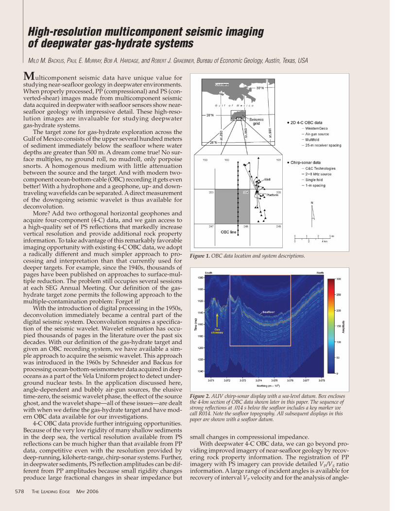
Figure 2. AUV chirp-sonar display with a sea-level datum. Box enclosesthe 4-km section of OBC data shown later in this paper. The sequence ofstrong reflections at .014 s below the seafloor includes a key marker wecall R014. Note the seafloor topography. All subsequent displays in thispaper are shown with a seafloor datum.

dependent reflectivity. Improved vertical resolution andnew rock property information are thus available with 4-COBC data. It is true that the surface multiple can interferewith PS reflection data. Fortunately we have found a sim-ple and effective approach to use multicomponent data toremove this multiple from horizontal-component data. Thecomplications normally encountered in seismic wave trans-mission to the target zone are not encountered because thethick water layer is a well behaved medium. Any trans-mission issues in the upper sediments constitute part of thegeologic signal rather than being a nasty problem that com-plicates the recovery of deeper target information.

The methods discussed in this paper are designed forgas-hydrate targets. They are not generally applicable fordeeper targets or for OBC data recorded on the continentalshelf or in shallow water. We conclude that deepwater gas-hydrate targets provide a delightful research opportunity.Our results to date have surprised us, and we anticipatemany future surprises as we proceed to more widely applythese concepts. In this paper, we illustrate results for 4-COBC data collected in the Gulf of Mexico at a water depthof about 850 m. We outline both the processing approachwe use and the rationale for this approach.

Imaging the gas-hydrate target zone. Our example data setincludes conventional 4-C OBC data and autonomousunderwater vehicle (AUV) chirp-sonar data over a 4-km linein the Green Canyon area on the northern slope of the gulf(Figure 1). The operational aspects of AUV systems will bedescribed later when we discuss Figure 16. For the present,we want to stress that only shallow sediments (depths of40–60 m) are revealed by AUV chirp-sonar data. An exam-ple AUV image is illustrated in Figure 2 after the data havebeen corrected to a sea-level datum.

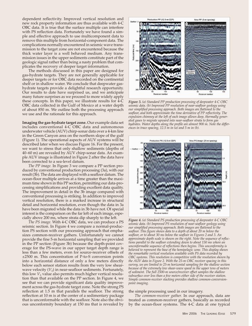
The PP image. In Figure 3 we compare a PP section pro-duced by conventional production processing (3a), with ourresult (3b). The data are displayed with a seafloor datum. Theocean-floor multiple arrives at a time greater than the maxi-mum time shown in this PP section, permitting our data-pro-cessing simplifications and providing excellent data quality.The improvement in detail in the 3b image compared withconventional processing is striking. In addition to improvedvertical resolution, there is a marked increase in structuraldetail and horizontal resolution, even though the data in 3ahave been migrated while the data in 3b have not. Of specialinterest is the comparison on the far left of each image, espe-cially above 200 ms, where strata dip sharply to the left.

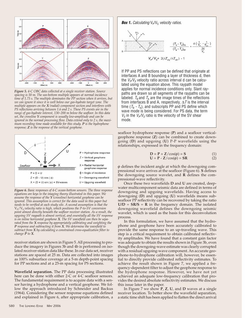
The PS image. With 4-C OBC data, we can produce a PSseismic section. In Figure 4 we compare a normal-produc-tion PS section with our processing approach that empha-sizes common-receiver gathers. Unfortunately we cannotprovide the fine 5-m horizontal sampling that we providedin the PP section (Figure 3b) because the depth-point cov-erage for the PS-wave in our upper target depth range isless than a few meters, even for source-receiver offsets of±2500 m. This concentration of P-to-S conversion pointsinto a horizontal distance of only a few meters directlybelow each sensor station results from the very low shear-wave velocity (VS) in near-seafloor sediments. Fortunately,this low VS value also permits much higher vertical resolu-tion than that available on the PP section. In Figure 4, wesee that we can provide significant data quality improve-ment across the gas-hydrate target zone. Note the strong PSreflection at 1.5 m that parallels the seafloor. The strongreflection at 10 m is at the center of a sedimentary packagethat is unconformable with the seafloor. Note also the obvi-ous unconformity boundary at 150 ms that is revealed by

the simple processing used in our imagery.The common-receiver gather. In our approach, data are

treated as common-receiver gathers, basically as recordedby the ocean-floor systems. The 4-C data at one typical

MAY 2006 THE LEADING EDGE 579

Figure 3. (a) Standard PP production processing of deepwater 4-C OBCseismic data. (b) Improved PP resolution of near-seafloor geology usingour simplified processing approach. Both images are flattened to theseafloor, and both approximate the time derivative of PP reflectivity. Theexpulsion chimney at the left of each image allows deep, thermally gener-ated gases to migrate upward into near-seafloor strata to form gashydrates. Water depths along the profile are almost 900 m. Note the differ-ences in trace spacing, 12.5 m in (a) and 5 m in (b).

Figure 4. (a) Standard PS production processing of deepwater 4-C OBCseismic data. (b) Improved PS resolution of near-seafloor geology usingour simplified processing approach. Both images are flattened to theseafloor. This figure shows data to a depth of about 20 m below theseafloor, or to about 30 ms below the seafloor in Figures 2 and 3. Anapproximate depth scale is shown on the right. Note the sequence of reflec-tions parallel to the seafloor extending down to about 150 ms where anunconformable sequence of reflections then begins. This unconformity isbelieved to represent the base of the hemipelagic zone. This display showsthe remarkable vertical resolution available with PS data recorded byOBC systems. This resolution is competitive with the resolution shown bythe AUV data in Figure 2. With the 25-m OBC receiver spacing in thissurvey, we are limited to 25-m horizontal sampling for the shallow sectionbecause of the extremely low shear-wave speed in the upper tens of metersof sediment. The full 2500-m source/receiver offset samples the shallowsubsurface over less than a few meters either side of the receiver station.Simple common-receiver stacking provides shallow common-conversion-point imaging.

receiver station are shown in Figure 5. All processing to pro-duce the imagery in Figures 3b and 4b is performed on iso-lated receiver-station data like these. In our data set, receiverstations are spaced at 25 m. Data are collected into imagesas 100% subsurface coverage at a 5-m depth-point spacingfor PP sections and at a 25-m spacing for PS sections.

Wavefield separation. The PP data processing illustratedhere can be done with either 2-C or 4-C seafloor sensors.The fundamental requirement is to acquire data with a sen-sor having a hydrophone and a vertical geophone. We fol-low the approach introduced by Schneider and Backus(1964). Considering the sensor response equations definedand explained in Figure 6, after appropriate calibration, a

seafloor hydrophone response (P) and a seafloor vertical-geophone response (Z) can be combined to create down-going (D) and upgoing (U) P-P wavefields using therelationships, expressed in the frequency domain:

D = P + Z/cos(φ) = S (1)U = P - Z/cos(φ) = SR (2)

φ defines the incident angle at which the downgoing com-pressional wave arrives at the seafloor (Figure 6). S definesthe downgoing source wavelet, and R defines the com-pressional-wave reflectivity.

Once these two wavefields D and U are created, deep-water multicomponent seismic data are defined in terms ofdowngoing and upgoing wavefields. Having access todowngoing (D) and upgoing (U) wavefields means sub-seafloor PP reflectivity can be recovered by taking the ratioU/D = SR/S = R in the frequency domain. The isolateddowngoing wavefield defines the downgoing seismicwavelet, which is used as the basis for this deconvolutionprocess.

In this formulation, we have assumed that the hydro-phone and geophone have been accurately calibrated toprovide the same response to an up-traveling wave. Thisstep is a critical requirement to obtain calibrated reflectiv-ity amplitudes. We have found that a constant gain factorwas adequate to obtain the results shown in Figure 3b, eventhough the downgoing-wave estimate was clearly corruptedwith a residual upgoing-wave component. An accurate geo-phone-to-hydrophone calibration will, however, be essen-tial to directly provide calibrated reflectivity estimates. Toachieve the result shown in Figure 7, we applied a fre-quency-dependent filter to adjust the geophone response tothe hydrophone response. However, we have not yetachieved an adequate low-frequency calibration that pro-vides the desired absolute reflectivity estimates. We discussthis issue later in the paper.

In Figure 7 we show P, Z, U, and D waves at a singlereceiver location. To better show the wavefield separation,a static time shift has been applied to flatten the direct arrival


Figure 6. Basic responses of 4-C ocean-bottom sensors. The three responseequations are keys to the imaging theory illustrated in this paper. Weassume the response of the Y (crossline) horizontal geophone can beignored. This assumption is correct for the data used in this paper butneeds to be verified at each study site. A second assumption is that theVP/VS velocity ratio is high, which positions the P-to-SV conversionpoint almost directly beneath the seafloor receiver station. As a result, theupgoing SV raypath is almost vertical, and essentially all the SV responseis on inline horizontal geophone X. The SV wavefield can then be sepa-rated from the X response by appropriately calibrating and weighting theP response and subtracting it from X. We determine the wavefield tosubtract from X by calculating a constrained cross-equalization filter tochange P to X.

Figure 5. 4-C OBC data collected at a single receiver station. Sourcespacing is 50 m. The sea-bottom multiple appears at normal incidencetime of 1.75 s. The multiple dominates the PP section when it arrives, butwe can ignore it since it is well below our gas-hydrate target zone. Themultiple appears on the X (radial) component section and interferes withPS reflections arriving between 1.6 and 2 s. These PS events are in therange of gas-hydrate interest, 130–200 m below the seafloor. In this dataset, the crossline Y component is usually low-amplitude and can beignored in the normal processing flow. Data extend only to 2 s, the maxi-mum recording time made available for this study. P is the hydrophoneresponse; Z is the response of the vertical geophone.

Box 1. Calculating VP/VS velocity ratios.

If PP and PS reflections can be defined that originate atinterfaces A and B bounding a layer of thickness d, thenthe VP/VS velocity ratio across interval d can be calcu-lated using the equation above. This raypath modelapplies for normal incidence conditions only. Slant ray-paths are drawn so all segments of the raypaths can belabeled. TB and TA are the image times of the reflectionsfrom interfaces B and A, respectively, ∆T is the intervaltime (TB - TA), and subscripts PP and PS define whichwave mode is being considered. For PS data, the termVS in the VP/VS ratio is the velocity of the SV shearmode.

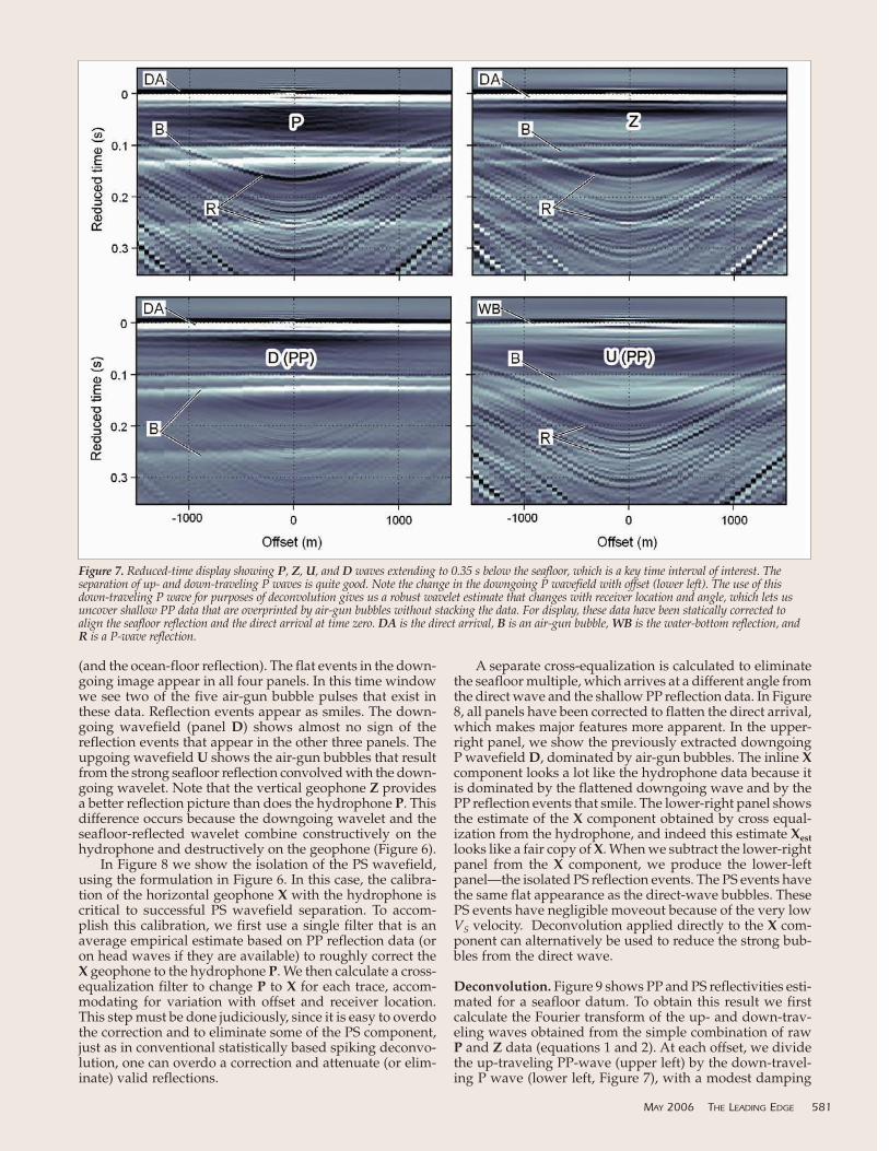
(and the ocean-floor reflection). The flat events in the down-going image appear in all four panels. In this time windowwe see two of the five air-gun bubble pulses that exist inthese data. Reflection events appear as smiles. The down-going wavefield (panel D) shows almost no sign of thereflection events that appear in the other three panels. Theupgoing wavefield U shows the air-gun bubbles that resultfrom the strong seafloor reflection convolved with the down-going wavelet. Note that the vertical geophone Z providesa better reflection picture than does the hydrophone P. Thisdifference occurs because the downgoing wavelet and theseafloor-reflected wavelet combine constructively on thehydrophone and destructively on the geophone (Figure 6).

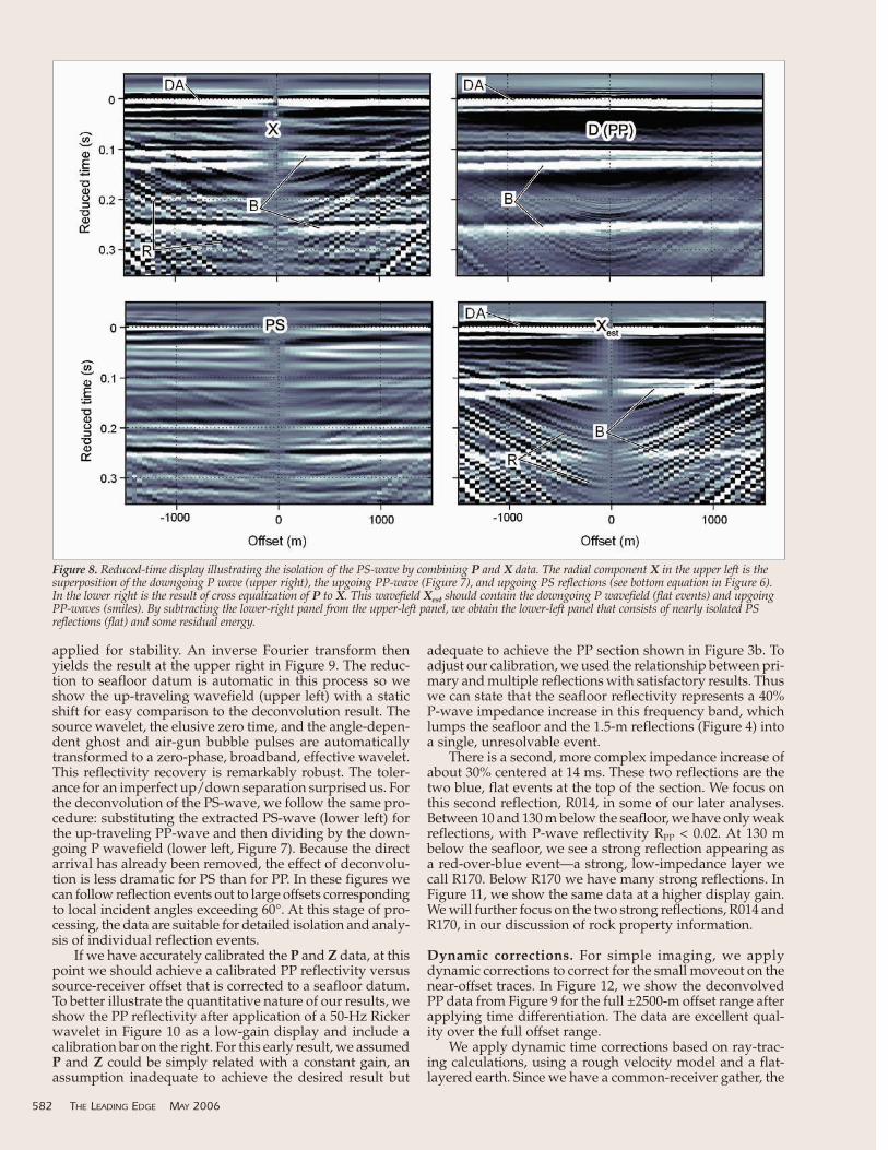
In Figure 8 we show the isolation of the PS wavefield,using the formulation in Figure 6. In this case, the calibra-tion of the horizontal geophone X with the hydrophone iscritical to successful PS wavefield separation. To accom-plish this calibration, we first use a single filter that is anaverage empirical estimate based on PP reflection data (oron head waves if they are available) to roughly correct theX geophone to the hydrophone P. We then calculate a cross-equalization filter to change P to X for each trace, accom-modating for variation with offset and receiver location.This step must be done judiciously, since it is easy to overdothe correction and to eliminate some of the PS component,just as in conventional statistically based spiking deconvo-lution, one can overdo a correction and attenuate (or elim-inate) valid reflections.

A separate cross-equalization is calculated to eliminatethe seafloor multiple, which arrives at a different angle fromthe direct wave and the shallow PP reflection data. In Figure8, all panels have been corrected to flatten the direct arrival,which makes major features more apparent. In the upper-right panel, we show the previously extracted downgoingP wavefield D, dominated by air-gun bubbles. The inline Xcomponent looks a lot like the hydrophone data because itis dominated by the flattened downgoing wave and by thePP reflection events that smile. The lower-right panel showsthe estimate of the X component obtained by cross equal-ization from the hydrophone, and indeed this estimate Xestlooks like a fair copy of X. When we subtract the lower-rightpanel from the X component, we produce the lower-leftpanel—the isolated PS reflection events. The PS events havethe same flat appearance as the direct-wave bubbles. ThesePS events have negligible moveout because of the very lowVS velocity. Deconvolution applied directly to the X com-ponent can alternatively be used to reduce the strong bub-bles from the direct wave.

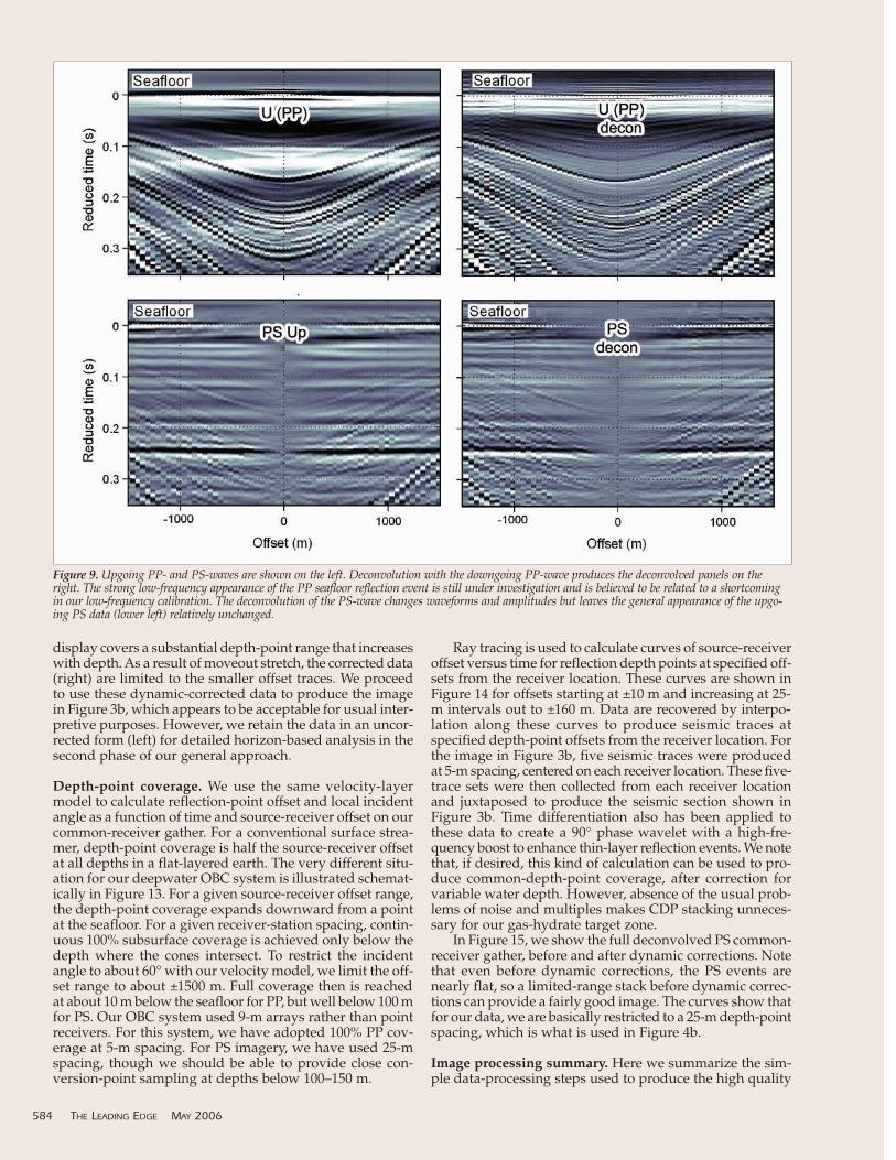
Deconvolution. Figure 9 shows PP and PS reflectivities esti-mated for a seafloor datum. To obtain this result we firstcalculate the Fourier transform of the up- and down-trav-eling waves obtained from the simple combination of rawP and Z data (equations 1 and 2). At each offset, we dividethe up-traveling PP-wave (upper left) by the down-travel-ing P wave (lower left, Figure 7), with a modest damping


Figure 7. Reduced-time display showing P, Z, U, and D waves extending to 0.35 s below the seafloor, which is a key time interval of interest. Theseparation of up- and down-traveling P waves is quite good. Note the change in the downgoing P wavefield with offset (lower left). The use of thisdown-traveling P wave for purposes of deconvolution gives us a robust wavelet estimate that changes with receiver location and angle, which lets usuncover shallow PP data that are overprinted by air-gun bubbles without stacking the data. For display, these data have been statically corrected toalign the seafloor reflection and the direct arrival at time zero. DA is the direct arrival, B is an air-gun bubble, WB is the water-bottom reflection, andR is a P-wave reflection.

applied for stability. An inverse Fourier transform thenyields the result at the upper right in Figure 9. The reduc-tion to seafloor datum is automatic in this process so weshow the up-traveling wavefield (upper left) with a staticshift for easy comparison to the deconvolution result. Thesource wavelet, the elusive zero time, and the angle-depen-dent ghost and air-gun bubble pulses are automaticallytransformed to a zero-phase, broadband, effective wavelet.This reflectivity recovery is remarkably robust. The toler-ance for an imperfect up/down separation surprised us. Forthe deconvolution of the PS-wave, we follow the same pro-cedure: substituting the extracted PS-wave (lower left) forthe up-traveling PP-wave and then dividing by the down-going P wavefield (lower left, Figure 7). Because the directarrival has already been removed, the effect of deconvolu-tion is less dramatic for PS than for PP. In these figures wecan follow reflection events out to large offsets correspondingto local incident angles exceeding 60°. At this stage of pro-cessing, the data are suitable for detailed isolation and analy-sis of individual reflection events.

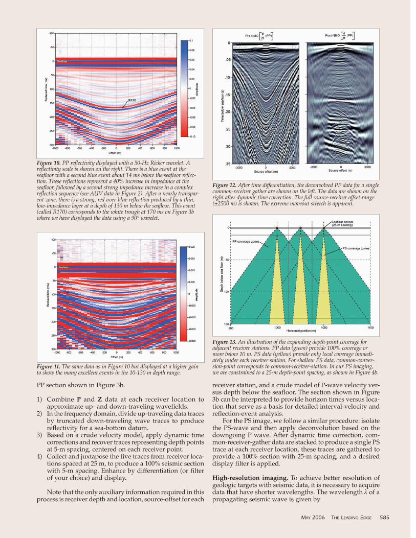
If we have accurately calibrated the P and Z data, at thispoint we should achieve a calibrated PP reflectivity versussource-receiver offset that is corrected to a seafloor datum.To better illustrate the quantitative nature of our results, weshow the PP reflectivity after application of a 50-Hz Rickerwavelet in Figure 10 as a low-gain display and include acalibration bar on the right. For this early result, we assumedP and Z could be simply related with a constant gain, anassumption inadequate to achieve the desired result but

adequate to achieve the PP section shown in Figure 3b. Toadjust our calibration, we used the relationship between pri-mary and multiple reflections with satisfactory results. Thuswe can state that the seafloor reflectivity represents a 40%P-wave impedance increase in this frequency band, whichlumps the seafloor and the 1.5-m reflections (Figure 4) intoa single, unresolvable event.

There is a second, more complex impedance increase ofabout 30% centered at 14 ms. These two reflections are thetwo blue, flat events at the top of the section. We focus onthis second reflection, R014, in some of our later analyses.Between 10 and 130 m below the seafloor, we have only weakreflections, with P-wave reflectivity RPP < 0.02. At 130 mbelow the seafloor, we see a strong reflection appearing asa red-over-blue event—a strong, low-impedance layer wecall R170. Below R170 we have many strong reflections. InFigure 11, we show the same data at a higher display gain.We will further focus on the two strong reflections, R014 andR170, in our discussion of rock property information.

Dynamic corrections. For simple imaging, we applydynamic corrections to correct for the small moveout on thenear-offset traces. In Figure 12, we show the deconvolvedPP data from Figure 9 for the full ±2500-m offset range afterapplying time differentiation. The data are excellent qual-ity over the full offset range.

We apply dynamic time corrections based on ray-trac-ing calculations, using a rough velocity model and a flat-layered earth. Since we have a common-receiver gather, the


Figure 8. Reduced-time display illustrating the isolation of the PS-wave by combining P and X data. The radial component X in the upper left is thesuperposition of the downgoing P wave (upper right), the upgoing PP-wave (Figure 7), and upgoing PS reflections (see bottom equation in Figure 6).In the lower right is the result of cross equalization of P to X. This wavefield Xest should contain the downgoing P wavefield (flat events) and upgoingPP-waves (smiles). By subtracting the lower-right panel from the upper-left panel, we obtain the lower-left panel that consists of nearly isolated PSreflections (flat) and some residual energy.

display covers a substantial depth-point range that increaseswith depth. As a result of moveout stretch, the corrected data(right) are limited to the smaller offset traces. We proceedto use these dynamic-corrected data to produce the imagein Figure 3b, which appears to be acceptable for usual inter-pretive purposes. However, we retain the data in an uncor-rected form (left) for detailed horizon-based analysis in thesecond phase of our general approach.

Depth-point coverage. We use the same velocity-layermodel to calculate reflection-point offset and local incidentangle as a function of time and source-receiver offset on ourcommon-receiver gather. For a conventional surface strea-mer, depth-point coverage is half the source-receiver offsetat all depths in a flat-layered earth. The very different situ-ation for our deepwater OBC system is illustrated schemat-ically in Figure 13. For a given source-receiver offset range,the depth-point coverage expands downward from a pointat the seafloor. For a given receiver-station spacing, contin-uous 100% subsurface coverage is achieved only below thedepth where the cones intersect. To restrict the incidentangle to about 60° with our velocity model, we limit the off-set range to about ±1500 m. Full coverage then is reachedat about 10 m below the seafloor for PP, but well below 100 mfor PS. Our OBC system used 9-m arrays rather than pointreceivers. For this system, we have adopted 100% PP cov-erage at 5-m spacing. For PS imagery, we have used 25-mspacing, though we should be able to provide close con-version-point sampling at depths below 100–150 m.

Ray tracing is used to calculate curves of source-receiveroffset versus time for reflection depth points at specified off-sets from the receiver location. These curves are shown inFigure 14 for offsets starting at ±10 m and increasing at 25-m intervals out to ±160 m. Data are recovered by interpo-lation along these curves to produce seismic traces atspecified depth-point offsets from the receiver location. Forthe image in Figure 3b, five seismic traces were producedat 5-m spacing, centered on each receiver location. These five-trace sets were then collected from each receiver locationand juxtaposed to produce the seismic section shown inFigure 3b. Time differentiation also has been applied tothese data to create a 90° phase wavelet with a high-fre-quency boost to enhance thin-layer reflection events. We notethat, if desired, this kind of calculation can be used to pro-duce common-depth-point coverage, after correction forvariable water depth. However, absence of the usual prob-lems of noise and multiples makes CDP stacking unneces-sary for our gas-hydrate target zone.

In Figure 15, we show the full deconvolved PS common-receiver gather, before and after dynamic corrections. Notethat even before dynamic corrections, the PS events arenearly flat, so a limited-range stack before dynamic correc-tions can provide a fairly good image. The curves show thatfor our data, we are basically restricted to a 25-m depth-pointspacing, which is what is used in Figure 4b.

Image processing summary. Here we summarize the sim-ple data-processing steps used to produce the high quality


Figure 9. Upgoing PP- and PS-waves are shown on the left. Deconvolution with the downgoing PP-wave produces the deconvolved panels on theright. The strong low-frequency appearance of the PP seafloor reflection event is still under investigation and is believed to be related to a shortcomingin our low-frequency calibration. The deconvolution of the PS-wave changes waveforms and amplitudes but leaves the general appearance of the upgo-ing PS data (lower left) relatively unchanged.

PP section shown in Figure 3b.

1) Combine P and Z data at each receiver location toapproximate up- and down-traveling wavefields.

2) In the frequency domain, divide up-traveling data tracesby truncated down-traveling wave traces to producereflectivity for a sea-bottom datum.

3) Based on a crude velocity model, apply dynamic timecorrections and recover traces representing depth pointsat 5-m spacing, centered on each receiver point.

4) Collect and juxtapose the five traces from receiver loca-tions spaced at 25 m, to produce a 100% seismic sectionwith 5-m spacing. Enhance by differentiation (or filterof your choice) and display.

Note that the only auxiliary information required in thisprocess is receiver depth and location, source-offset for each

receiver station, and a crude model of P-wave velocity ver-sus depth below the seafloor. The section shown in Figure3b can be interpreted to provide horizon times versus loca-tion that serve as a basis for detailed interval-velocity andreflection-event analysis.

For the PS image, we follow a similar procedure: isolatethe PS-wave and then apply deconvolution based on thedowngoing P wave. After dynamic time correction, com-mon-receiver-gather data are stacked to produce a single PStrace at each receiver location, these traces are gathered toprovide a 100% section with 25-m spacing, and a desireddisplay filter is applied.

High-resolution imaging. To achieve better resolution ofgeologic targets with seismic data, it is necessary to acquiredata that have shorter wavelengths. The wavelength λ of apropagating seismic wave is given by


Figure 12. After time differentiation, the deconvolved PP data for a singlecommon-receiver gather are shown on the left. The data are shown on theright after dynamic time correction. The full source-receiver offset range(±2500 m) is shown. The extreme moveout stretch is apparent.

Figure 13. An illustration of the expanding depth-point coverage foradjacent receiver stations. PP data (green) provide 100% coverage ormore below 10 m. PS data (yellow) provide only local coverage immedi-ately under each receiver station. For shallow PS data, common-conver-sion-point corresponds to common-receiver-station. In our PS imaging,we are constrained to a 25-m depth-point spacing, as shown in Figure 4b.

Figure 10. PP reflectivity displayed with a 50-Hz Ricker wavelet. Areflectivity scale is shown on the right. There is a blue event at theseafloor with a second blue event about 14 ms below the seafloor reflec-tion. These reflections represent a 40% increase in impedance at theseafloor, followed by a second strong impedance increase in a complexreflection sequence (see AUV data in Figure 2). After a nearly transpar-ent zone, there is a strong, red-over-blue reflection produced by a thin,low-impedance layer at a depth of 130 m below the seafloor. This event(called R170) corresponds to the white trough at 170 ms on Figure 3bwhere we have displayed the data using a 90° wavelet.

Figure 11. The same data as in Figure 10 but displayed at a higher gainto show the many excellent events in the 10-130 m depth range.

λ = V/f (3)

where V is propagation velocity and f is frequency. Thisequation shows there are two ways to reduce an imagingwavelength λ: either (1) increase f, or (2) reduce V.

Short-wavelength option 1: Increasing the frequency with AUVtechnology. If deepwater strata are illuminated with conven-tional air-gun sources towed at the sea surface, we can improveupon conventional imaging as illustrated in Figure 3a, but res-olution is still limited by the long-wavelength spectrum of theair gun data. An approach now used to acquire deepwater,short-wavelength PP data for studying near-seafloor geologyis to use an AUV system (Figure 16). An AUV travels approx-imately 50 m above the seafloor and illuminates subseafloorstrata with chirp-sonar pulses having a frequency bandwidthof 2–8 kHz. This increase in signal frequency shortens PPwavelengths by a factor of almost 100 compared to the wave-lengths of a conventional air-gun signal used for oil and gasexploration. The result is an illuminating wavefield havingwavelengths of a fraction of a meter when near-seafloor veloc-ity VP is 1500–1600 m/s, a common range of VP for deepwa-ter, near-seafloor sediments across gas-hydrate target intervals.An example of an AUV chirp-sonar image acquired at the loca-tion of our OBC data is shown in Figure 2, with a detail zoomshown in Figure 17. Figure 18 shows the AUV data over the

4-km study line as collected (below) and then as flattened toa sea-bottom datum (above). These high-frequency signalspenetrate only 40–60 m into the seafloor, but they image bed-ding of meter-scale thicknesses across this near-seafloor imagespace. The horizontal sampling of 1 m or less enhances thevalue of AUV data.

Short-wavelength option 2: Reducing the velocity by switch-ing to PS imaging. It is not possible to acquire shorter-wave-length PP data by reducing VP in a seismic propagationmedium. The value of VP within a system of targeted stratais fixed and cannot be altered. However, a seismic imagingeffort can switch from the conventional approach of usingthe PP seismic mode and focus on using another wave modethat does have reduced velocity within near-seafloor strata.That logic has great benefit for imaging deepwater, near-seafloor geology when the imaging effort focuses on PS datarather than on PP data. Across many deepwater areas, par-ticularly deepwaters of the Gulf of Mexico, VS in near-seafloorsediments tends to be 20–50 times less than VP. Thus if PPand PS data have equivalent frequency content, which theydo for shallow penetration distances into the seafloor, PS datawill have wavelengths much shorter than PP wavelengths.

The illuminating wavefield that created the PS data shownin Figure 4 was a 10–150 Hz P wavefield produced by a con-ventional air-gun array positioned at the sea surface, the


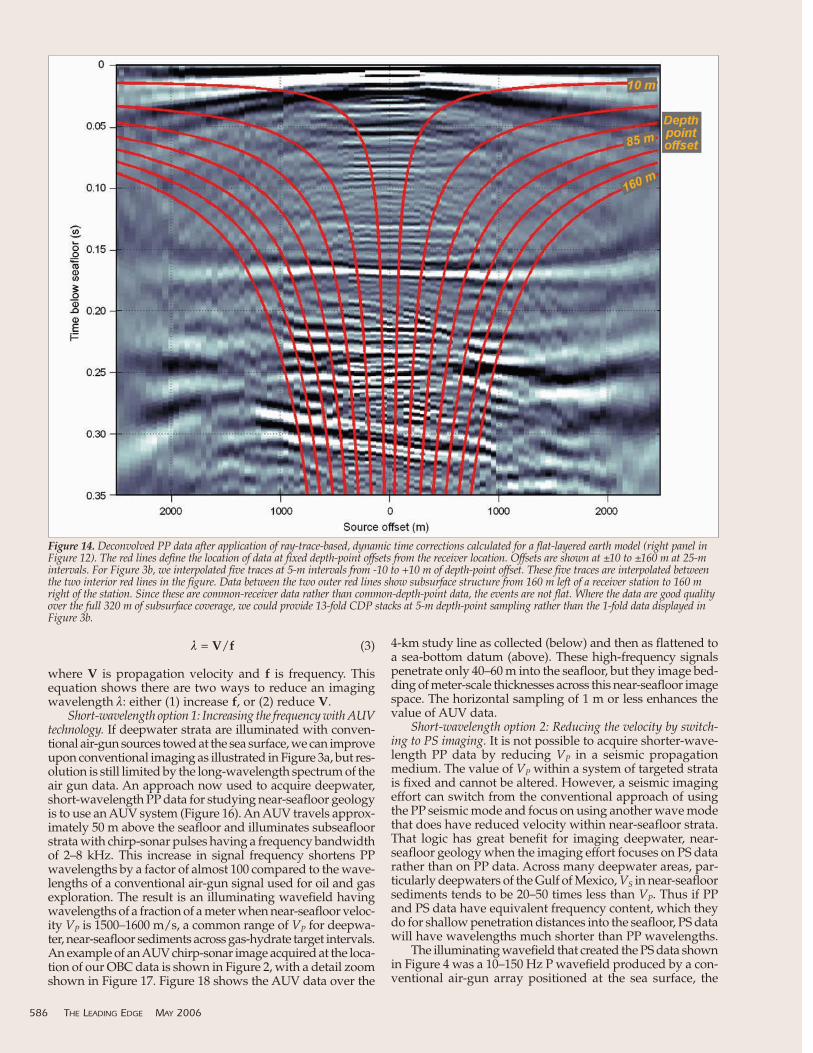
Figure 14. Deconvolved PP data after application of ray-trace-based, dynamic time corrections calculated for a flat-layered earth model (right panel inFigure 12). The red lines define the location of data at fixed depth-point offsets from the receiver location. Offsets are shown at ±10 to ±160 m at 25-mintervals. For Figure 3b, we interpolated five traces at 5-m intervals from -10 to +10 m of depth-point offset. These five traces are interpolated betweenthe two interior red lines in the figure. Data between the two outer red lines show subsurface structure from 160 m left of a receiver station to 160 mright of the station. Since these are common-receiver data rather than common-depth-point data, the events are not flat. Where the data are good qualityover the full 320 m of subsurface coverage, we could provide 13-fold CDP stacks at 5-m depth-point sampling rather than the 1-fold data displayed inFigure 3b.


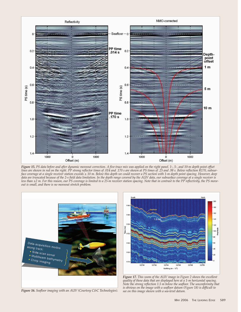
Figure 15. PS data before and after dynamic moveout correction. A five-trace mix was applied on the right panel. 1-, 5-, and 10-m depth point offsetlines are shown in red on the right. PP strong reflector times of .014 and .170 s are shown at PS times of .25 and .98 s. Below reflection R170, subsur-face coverage at a single receiver station exceeds ± 10 m. Below this depth we could recover a PS section with 1-m depth point spacing. However, deepdata are truncated because of the 2-s field data limitation. In the depth range covered by the AUV data, our subsurface coverage at a single receiver isless than ±2 m. For this reason, our PS coverage is limited to a 25-m receiver station spacing. Note that in contrast to the PP reflectivity, the PS move-out is small, and there is no moveout stretch problem.

Figure 16. Seafloor imaging with an AUV (Courtesy C&C Technologies).

Figure 17. This zoom of the AUV image in Figure 2 shows the excellentquality of these data that are displayed here at a 1-m horizontal spacing.Note the strong reflection 1.5 m below the seafloor. The unconformity thatis obvious on the image with a seafloor datum (Figure 18) is difficult tosee on this image shown with a sea-level datum.

same source used to produce the PP images in Figure 3.Because VS in near-seafloor sediment along this OBC profileis less than 100 m/s, the PS data have wavelengths less than1 m just as do the high-frequency AUV chirp-sonar data inFigure 17, even though the PS data are low frequency.

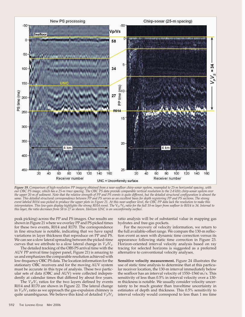
In Figure 19, we compare the shallow PS image with thechirp-sonar image, which has been resampled to 25-m spac-ing to correspond to the PS section. The event at 1.5 mappears at 2 ms on the PP chirp-sonar section and at 60 mson the PS image, implying a VP/VS ratio of ~60. The 10-mdeep event at 14 ms on the PP section appears at 250 ms onthe PS data. Note the unconformity UNC at ~150 ms on PSthat ties to ~7 or 8 ms on PP, with the latter time positionbetter seen in the upper panel of Figure 18. This unam-biguous registration of our PS data to the chirp-sonar datain the shallow section is both remarkable and surprising.

Unfortunately these high-resolution PS images cannot beextended to great subseafloor depths. PS wavelengthsincrease, and thus PS resolution decreases, with increasingdepth. At this location, the VP/VS ratio decreases sharply

below 20 m to about 8 and reduces to 4 and less below 150 mwhere PS and PP resolution is more comparable. However,for deepwater strata close to the seafloor, the spatial resolu-tion of PS data is most impressive. The contrast in the reso-lution of companion-mode PP and PS 4-C OBC imagesexhibited by these comparisons is, to some people, amazing.

Rock properties. For detailed analysis of these data, wefocus on major reflection horizons and apply static timecorrections to these targeted events based on raypath cal-culations. Two strong events were analyzed on this data set.One is the R014 event shown in Figure 19 at 14 ms on theAUV PP section and at 250 ms on the PS section. The sec-ond, a strongly reflecting, thin, low-speed layer 130 m belowthe seafloor, is shown in Figure 20. This event, R170, is at170 ms on PP and at about 980 ms on PS. Note the compa-rable waveforms on the OBC PP and PS reflections. InFigures 19 and 20, the correspondence between PP and PSdetailed structural variations is remarkable. To see this cor-respondence in greater detail, we picked the events (simple


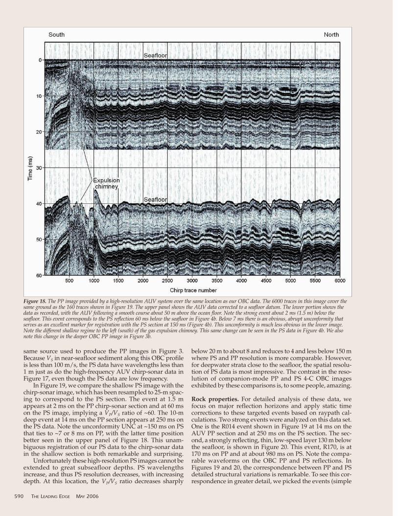
Figure 18. The PP image provided by a high-resolution AUV system over the same location as our OBC data. The 6000 traces in this image cover thesame ground as the 160 traces shown in Figure 19. The upper panel shows the AUV data corrected to a seafloor datum. The lower portion shows thedata as recorded, with the AUV following a smooth course about 50 m above the ocean floor. Note the strong event about 2 ms (1.5 m) below theseafloor. This event corresponds to the PS reflection 60 ms below the seafloor in Figure 4b. Below 7 ms there is an obvious, abrupt unconformity thatserves as an excellent marker for registration with the PS section at 150 ms (Figure 4b). This unconformity is much less obvious in the lower image.Note the different shallow regime to the left (south) of the gas expulsion chimney. This same change can be seen in the PS data in Figure 4b. We alsonote this change in the deeper OBC PP image in Figure 3b.

peak picking) across the PP and PS images. Our results areshown in Figure 21 where we overlay PP and PS picked timesfor these two events, R014 and R170. The correspondencein fine structure is notable, indicating that we have rapidvariations in layer thickness that reproduce on PP and PS.We can see a slow lateral spreading between the picked-timecurves that we attribute to a slow lateral change in VP/VS.

The detailed tracking of the OBS PS arrival time with theAUV PP arrival time (upper panel, Figure 21) is amazing tous and emphasizes the comparable resolution achieved withlow-frequency OBC PS data. The location information for thestationary OBC receivers and for the moving AUV systemmust be accurate in this type of analysis. These two partic-ular sets of data (OBC and AUV) were collected indepen-dently at calendar times that differed by about five years.

The VP/VS ratios for the two layers defined by eventsR014 and R170 are shown in Figure 22. The lateral changein VP/VS ratio as we approach the gas-expulsion chimney isquite unambiguous. We believe this kind of detailed VP/VS

ratio analysis will be of substantial value in mapping gashydrates and free-gas pockets.

For the recovery of velocity information, we return tothe full available-offset range. We compare the 130-m reflec-tion event as seen with dynamic time correction versus itsappearance following static time correction in Figure 23.Horizon-oriented interval velocity analysis based on raytracing for selected horizons is suggested as a preferredalternative to conventional velocity analyses.

Sensitive velocity measurement. Figure 24 illustrates theuse of static time analysis to determine that at this particu-lar receiver location, the 130-m interval immediately belowthe seafloor has an interval velocity of 1550–1560 m/s. Thissensitivity of less than 0.5% in interval velocity over a 130-m thickness is notable. We usually consider velocity uncer-tainty to be much greater than traveltime uncertainty inestimates of depth and thickness. This 0.5% sensitivity tointerval velocity would correspond to less than 1 ms time


Figure 19. Comparison of high-resolution PP imagery obtained from a near-seafloor chirp-sonar system, resampled to 25-m horizontal spacing, withour OBC PS image, which has a 25-m trace spacing. The OBC PS data provide comparable vertical resolution to the 2-8 kHz chirp-sonar system overthe upper 20 m of sediment. Note that the relative strength of PP and PS events is quite different, but the detailed structural configuration is almost thesame. This detailed structural correspondence between PP and PS serves as an excellent basis for depth registering PP and PS sections. The strongevent labeled R014 was picked to produce the upper plots in Figure 21. At this near-seafloor level, the OBC PP data lack the resolution to make thisinterpretation. This low-gain display highlights the strong R014 event. The VP/VS ratio for the full 10-m layer from seafloor to R014 is 34. Internal tothis layer, the ratio decreases from 58 to 27 as shown. Horizon UNC is an unconformity surface.

error in determining interval thickness. We believe gas-hydrate targets will permit the observation of local intervalvelocities with unusual sensitivity.

In Figure 25 we show the static-corrected R170 PP andPS reflection events on a single common-receiver gather. Thisdisplay provides QC opportunities and a basis for furtherdetailed interpretation. Various approaches to interpretationare under investigation. We expect to be able to recoverdetailed vertical and lateral variations in VP/VS in gas-hydrate target zones by picking specific, registered-hori-zon, arrival times on the PP and PS imagery as was donefor two particular horizons in Figure 21. When we do nothave access to AUV data, we will be limited in vertical res-olution because of the limitations of OBC PP resolution.

Hydrophone-to-geophone calibration. To achieve a properseparation of up- and down-traveling compressional wave-fields, a frequency-dependent relationship between hydro-phone and geophone responses to a unidirectional wavefieldmust first be applied to 4-C OBC data. We believe that thebest approach to this calibration is the use of waves thatarrive prior to the direct arrival. Head waves at far offsetsshould provide a clean upgoing wavefield. Unfortunately,in all of our work to date we have had access only to dataarriving before 2 s traveltime, so we have not had this cal-ibration method available. We have recently gained accessto OBC data on the Gulf of Mexico slope and in the BarentsSea that include far-offset data. We hope to use head wavesto improve calibrated reflectivity with these new data, par-ticularly at low frequencies. If successful, this calibrated


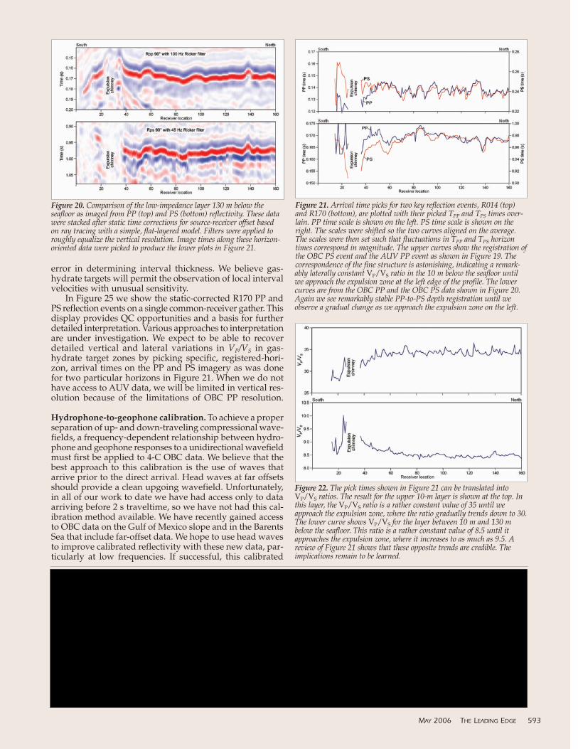
Figure 21. Arrival time picks for two key reflection events, R014 (top)and R170 (bottom), are plotted with their picked TPP and TPS times over-lain. PP time scale is shown on the left. PS time scale is shown on theright. The scales were shifted so the two curves aligned on the average.The scales were then set such that fluctuations in TPP and TPS horizontimes correspond in magnitude. The upper curves show the registration ofthe OBC PS event and the AUV PP event as shown in Figure 19. Thecorrespondence of the fine structure is astonishing, indicating a remark-ably laterally constant VP/VS ratio in the 10 m below the seafloor untilwe approach the expulsion zone at the left edge of the profile. The lowercurves are from the OBC PP and the OBC PS data shown in Figure 20.Again we see remarkably stable PP-to-PS depth registration until weobserve a gradual change as we approach the expulsion zone on the left.

Figure 22. The pick times shown in Figure 21 can be translated intoVP/VS ratios. The result for the upper 10-m layer is shown at the top. Inthis layer, the VP/VS ratio is a rather constant value of 35 until weapproach the expulsion zone, where the ratio gradually trends down to 30.The lower curve shows VP/VS for the layer between 10 m and 130 mbelow the seafloor. This ratio is a rather constant value of 8.5 until itapproaches the expulsion zone, where it increases to as much as 9.5. Areview of Figure 21 shows that these opposite trends are credible. Theimplications remain to be learned.

Figure 20. Comparison of the low-impedance layer 130 m below theseafloor as imaged from PP (top) and PS (bottom) reflectivity. These datawere stacked after static time corrections for source-receiver offset basedon ray tracing with a simple, flat-layered model. Filters were applied toroughly equalize the vertical resolution. Image times along these horizon-oriented data were picked to produce the lower plots in Figure 21.

reflectivity may allow direct estimates ofP-wave impedance across gas-hydrate tar-get zone. For some results in this paper, asingle empirically-derived filter was usedto correct for the average response differ-ence between hydrophone and geophone.A simple constant factor relating P and Zwas adequate to produce the result inFigure 3b. In Figures 10 and 11 we showfiltered PP reflectivity in which the cali-bration is based on independent estimatesof primary-to-multiple relationships. Wehope to achieve this same reflectivity cali-bration directly with improved hydro-phone-geophone calibration. In ourcurrent results, we observe features of theseabottom reflection that are puzzling,including suggestions of a very low P-wavevelocity. Further, though we are not con-cerned with surface multiples, the upper10 m of sediment is likely a strong interbed-multiple generator. Our reflectivity cali-bration is quite sensitive to the calibrationof relative-component response, whereasour imagery and reflection results are not.

PZ combinations. Relationships betweenthe usual production processing that cre-ates standard “PZ” traces and the up/downwavefield separation that we employ hereare not entirely clear. Different contractorsuse a variety of approaches to produce a PZ


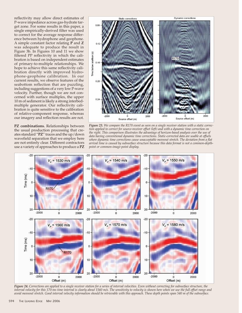
Figure 23. We compare the R170 event as seen on a single receiver station with a static correc-tion applied to correct for source-receiver offset (left) and with a dynamic time correction onthe right. This comparison illustrates the advantage of horizon-based analysis over the use ofdata having conventional dynamic time corrections. Static-corrected data are usable at offsetswhere dynamic time corrections cause unacceptable moveout stretch. The deviation from a flatarrival time is caused by subsurface structure because this data format is not a common-depth-point or common-image-point display.

Figure 24. Corrections are applied to a single receiver station for a series of interval velocities. Even without correcting for subsurface structure, theinterval velocity for this 170-ms time interval is clearly about 1560 m/s. The sensitivity to velocity is shown here when we use the full offset range andavoid moveout stretch. Good interval velocity information should be retrievable with this approach. These depth points span 540 m of the subsurface.

trace, with their objective usually being to empirically min-imize water reverberations. However, water reverberationsare not a concern for deepwater gas-hydrate target zones.

In any case, to achieve the results described in this paper,one must start with hydrophone and geophone data and prop-erly combine P and Z sensor responses.

Common-receiver-point processing. The confinement of ourprocessing to common-receiver gathers to produce our PP andPS images is of first-order significance. We also could applya slant-stack technique among shots for a given receiver. Thismodification would eliminate the variation in incidence anglewith time below the seafloor and might be advantageous. Weplan to try this modification in the next development round.

Seafloor datum is important. The use of a seafloor datumarises automatically from our approach to the deconvolutionprocess. Our data can be adjusted to a sea-level datum byapplying a static time shift to the sections shown in Figures 3and 4. Clearly a seafloor datum is convenient for dealing witha velocity model that depends on depth below the seafloor.Further, we believe a seafloor datum has significant interpre-tive advantages. For example, the bottom-simulating reflec-tion (BSR) related to many gas-hydrate systems outside theGulf of Mexico tends to parallel the seafloor, so a seafloordatum is particularly appropriate for recognizing BSR events.In Figures 4 and 18 we point out the improved visibility ofthe first reflections that are unconformable with the oceanfloor when a seafloor datum is used. Also, unless one dynam-ically corrects the vertical time scale for the PS section toaccurately agree with PP time, significant distortions occurin apparent PP and PS structure. Such distortions hurt ourability to depth register PP and PS data, and an accuratedepth registration is required before we can effectively use4-C OBC data. We have found that we are able to depth reg-ister standard production sections of PP and PS data much

more readily after correctingboth PP and PS data from theirstandard sea-level-datum pre-sentations to seafloor-datumpresentations.

Registration of PP and PS data.For a meaningful joint-inter-pretation of PP and PS reflec-tion data, depth registration ofPP and PS reflection time is fun-damental. In the gas-hydratetarget zone, with its very highVP/VS ratio, depth registrationis different from the usual case.In this example, our ability tounambiguously register OBCPS data to the totally differentPP chirp-sonar data for theR014 reflection (Figure 19) is aremarkable accomplishment.The unambiguous correspon-dence of the R170 event on PPand PS OBC data is also notable(Figures 20 and 21). These twoparticular correlations couldnot be achieved on normal pro-duction data, nor were theyachieved by a casual interpre-tation of our improved imageswhen we used conventional

approaches. We provide some comments on this depth reg-istration for the gas-hydrate target zone.

First, starting at the seafloor, we have a zone of reflectorsthat parallel the ocean floor, underlain by a layer sequenceunconformable to the seafloor and having sharp lateral vari-ations of arrival time below the seafloor (Figure 19). The onsettime of unconformity surface UNC in this figure and the cor-respondence of the unconformable structure immediatelybelow surface UNC provide an unambiguous PP to PS reg-istration. We can now flatten both PP and PS on this lowersequence and find the next unconformity. This dependenceon successive sequence flattening is a powerful approach toPP and PS depth registration when we have such extremedifferences in VP and VS.

Second, in this environment of high VP/VS values, largeVS contrasts can produce strong PS events but only weak PPevents. However, a strong PP reflection is likely to also appearas a strong PS reflection. Low-gain displays are thus helpfulin identifying these strong events, as illustrated in Figures 18and 19. Note that these marker reflections do not stand out inthe typical display that is aimed at showing all reflectors,whether strong or weak. These strong-amplitude reflectionsare also key events for detailed geologic analysis.

Finally, the detailed picked times on strong events providean excellent further basis for registration, as shown in Figure21. Given these picked times, we can fit PP times to PS timesand determine appropriate VP/VS relationships. For the R014reflection, we calculate an interval VP/VS value of 34 and alocal VP/VS value of 27 (Figure 19). For the R170 event, theinterval VP/VS value is 8, and the local VP/VS value is 7 (seeBox 1).

Shear-wave static corrections. In production OBC process-ing of PS data, shallow shear-wave statics are often a majorproblem. With the shallow geologic control demonstratedhere, we can provide important shallow information to assist


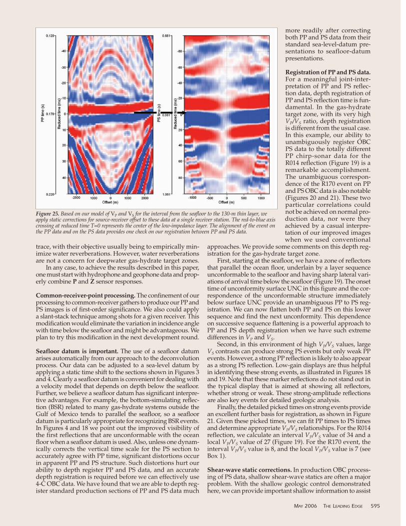
Figure 25. Based on our model of VP and VS for the interval from the seafloor to the 130-m thin layer, weapply static corrections for source-receiver offset to these data at a single receiver station. The red-to-blue axiscrossing at reduced time T=0 represents the center of the low-impedance layer. The alignment of the event onthe PP data and on the PS data provides one check on our registration between PP and PS data.

static analyses. Starting with the R170 event, we note that thePP and PS times overlay very well, except for the trend as weapproach the expulsion zone (Figure 21). This information canserve as a basis for shear-wave corrections for deeper data. Inour example OBC line, the shear-wave statics along the north-ern 3 km of the profile we have studied do not seem to beimportant. We expect to see stronger variations as we workwith more data locations.

Comparison with VSP systems. The processing of a 4-C OBCcommon-receiver gather can be compared to the processingof a vertical seismic profile (VSP) where reflection informa-tion is recovered from strata immediately beneath the VSP ver-tical array. In a VSP, we rarely have a hydrophone. Instead,the separation of up- and down-traveling wave is accom-plished by processing data acquired with a vertical array of3-C geophones. The use of the down-traveling wave as thewavelet for the VSP deconvolution process is analogous to theapproach we use here. Our approach to the dynamic correc-tion and recovery of a set of traces at several fixed offsets froma seafloor receiver station is also similar, at least in principal,to the traditional VSP-to-CDP transform used for offset VSPsources. In either case (deepwater OBC data or deep-well VSPdata), we have a great disparity between the length of the ray-path from source to target and the length of the raypath fromtarget to receiver. For the reader knowledgeable in VSP pro-cessing, this comparison may be helpful in understanding theOBC approach used here. Unfortunately, in VSP applicationswe do not have a line of wells at 25-m intervals like we havewith our deepwater receivers in OBC applications.

Conclusion. Deepwater multicomponent seismic data haveapplications for studying near-seafloor geology with a detailthat has not been appreciated or implemented across the geo-physical industry. The use of multicomponent data is par-ticularly important for evaluating deepwater gas-hydratesystems, which is our emphasis. Using 4-C OBC data forgeomechanical analyses of the seafloor is an obvious exten-sion of 4-C OBC technology that needs to be exploited. Suchgeotechnical applications will allow geophysicists to becomevaluable technical allies with engineers who have to under-stand seafloor stability across areas where deepwater facil-ities will be constructed.

Suggested reading. “Ocean-bottom seismic measurements offthe California coast” by Schneider and Backus (Journal ofGeophysical Research, 1964). “Enhanced PS-wave images of deep-water, near-seafloor geology from 2D, 4-C OBC data in the Gulfof Mexico” by Backus et al. (SEG 2005 Expanded Abstracts). TLE

Acknowledgments: Statoil, DOE NETL (contract DE-PS26-05NT42405),the Gas Hydrates Research Consortium at the University of Mississippi(DOE NETL contract DE-FC26-02NT41628), and MMS (contract0105CT39388) all contributed funding to support our research. Seismicdata were provided by WesternGeco. AUV data were provided throughMMS contract 1435-01-99-CA-30951 and the Gas Hydrates ResearchConsortium at the University of Mississippi.

Corresponding author: [email protected]


Documents

High-resolution multicomponent seismic imaging of ... · PDF fileHigh-resolution multicomponent seismic imaging of deepwater gas-hydrate systems MILOM. BACKUS, ... into a horizontal