High School Environments, STEM Orientations, and the

Gender Gap in Science and Engineering Degrees∗

Joscha Legewie and Thomas A. DiPrete

Columbia University and University of Wisconsin - Madison Madison

July 21, 2011

Abstract

This study examines two important and related dimensions of the persisting gender gap in science,

technology, engineering, and mathematics (STEM) bachelor degrees: First, the life-course timing

of a stable gender gap in STEM orientation, and second, variations in the gender gap across

high schools. We build on existing psychological and sociological gender theories to develop a

theoretical argument about the development of STEM orientations during adolescence and the

potential influence of the local high school environment on the formation of STEM orientations by

females and males. Using the National Education Longitudinal Study (NELS), we then decompose

the gender gap in STEM bachelor degrees and show that the solidification of the gender gap in

STEM orientations is largely a process that occurs during the high school years. Far from being

a fixed attribute of adolescent development, however, we find that the size of the gender gap in

STEM orientation is quite sensitive to local high school influences; going to school at a high school

that is supportive of a positive orientation by females towards math and science can reduce the

gender gap in STEM bachelor degrees by 25% or more.

∗This project was supported by Award Number R01EB010584 from the National Institute Of Biomedical ImagingAnd Bioengineering. The content is solely the responsibility of the authors and does not necessarily represent the officialviews of the National Institute Of Biomedical Imaging And Bioengineering or the National Institutes of Health.

Introduction

When then-Harvard President Lawrence Summers pointed at innate differences between men and

women as a possible explanation for women’s under-representation in high level science positions, he

sparked an intense public controversy that mirrors a continuing debate in the scientific community.

Despite the striking reversal of the gender gap in educational attainment (Buchmann and DiPrete

2006) and the near gender parity in math performance (Hyde et al. 2008), women still pursue science,

technology, engineering, and mathematics (STEM) degrees at much lower rates than their male peers

do. Figure 1 illustrates these trends. It shows, on the one hand, how women have made impressive

gains in college attainment compared to men and now clearly outnumber men among college graduates

in recent decades. On the other hand, women continue to lag behind in terms of bachelor degrees

awarded in the ’quantitative’ sciences (illustrated in the graph for different STEM sub-fields).1 This

persistent pattern of gender inequality in college science majors and the implications for later career

choices and labor market earnings has been a major concern for scientist and policy-makers alike.

Such differences are not only relevant for the representation of women in high income and prestigious

jobs and as such for gender equality in general but also for the supply of qualified labor in science

oriented jobs, which is often regarded as a linchpin for the future of the US economy in an increasingly

competitive global environment.

In this paper, we explore two important and related dimensions of the persisting gender gap in

STEM degrees. The first dimension is the timing of the emergence of a gender gap in orientation

towards STEM fields. Our analysis of the middle-school through college phase of the educational life

course reveals that the high school years play a major role in shaping gendered orientations toward

science and engineering. The second dimension concerns the impact of the high school environment

on the development of these orientations during the decisive high school years. In particular, we use

multilevel models to document how the gender gap in STEM orientation in twelfth grade varies across

high schools, and we estimate the causal effect of the high school curriculum on the gender gap in

STEM orientation. Far from being a fixed attribute of adolescent development, we find that the size

of the gender gap in STEM orientation is quite sensitive to local high school influences; going to school

in a high school that is supportive of a positive orientation by females towards math and science can

reduce the gender gap in STEM bachelor degrees by 25% or more. Together these two dimensions

of timing and local environmental influence extend existing theories and open concrete avenues for

policy intervention.1Exceptions to this trend are the biological, biomedical and life sciences, in which women today outnumber men.

1

Figure 1: Gender Gap in Bachelor Degrees Awarded by Field of Study, 1969-2007

1970 1980 1990 2000

0.0

0.5

1.0

1.5

2.0

2.5

Year

Fem

ale/

Mal

e O

dds

Rat

io

Female Advantage

Male Advantage

All Fields(incl. non-science)

Engineering and Engin. Tech.

biological and biomedical sciences

Mathematics and Statistics

Physical Sciences and Sci. Tech.

Source: Digest of Educational Statistics 2009, Table 268, 299, 303, 305, 312 and 313

We begin by developing a theoretical argument about the development of STEM orientations

during adolescence, and the potential influence of the local environment on the formation of STEM

orientations by females and males. While acknowledging the importance of the global environment,

we argue that local environments centrally affect the strength and salience of gender stereotypes

about math and science. Their influence operates mainly through two important processes. First,

peers, parents and teachers – all important actors in the local environment – support and encourage

certain career paths for boys and girls while disparaging others. Second, the influence of gender

stereotypes about STEM occupations depends on the level of exposure to STEM academic courses

and to information about STEM fields and STEM occupations. Both arguments imply that the size

of the gender gap in STEM bachelor degrees is shaped to a considerable extent by the character of the

high school environment. Variations in this environment will therefore affect the size of the gender

gap in STEM orientations.

We then turn to an empirical examination of the timing and the local variation across high schools.

First, we decompose the gender gap in STEM bachelor degrees into various pathways to examine the

emergence and solidification of gender differences in the orientation towards science and engineering in

the adolescent life course. In particular, we use the National Education Longitudinal Study (NELS)

to follow the 1988 cohort of eighth grade students through adolescence and young adulthood, and

observe how orientations towards STEM fields emerge and change from eighth grade through college.

2

We find that the substantial gender gap in eighth grade orientation is relatively inconsequential for

the persisting gender gap in STEM degrees at the completion of college. Instead, the high school

years play a major role in shaping gendered orientations towards science and engineering. Second, we

examine the role of the high school for this decisive period. In particular, we use multilevel models to

document how the gender gap in STEM orientation at the end of high school varies across high schools,

and we estimate the causal effect of high school curriculum on the gender gap in STEM orientation.

The results show substantial variation in the gender gap in STEM orientation across schools, which

supports our argument that the local environment plays a major role in shaping these orientations

among boys and girls. The significant effect of high school curriculum on the gender gap in STEM

orientation provides the beginning of an understanding about the source of the high school effect.

Our results imply that the gender gap could be considerably reduced if high school environments were

reshaped to model those high schools that are most supportive of female interest and competency in

science and mathematics.

Explanations for the Persisting Gender Gap in STEM Degrees

The most prominent explanations of the persisting gender gap in STEM degrees revolve around two

issues. First, the debate about gender differences in math ability continues to the present day even

though the gender gap in math performance has largely closed. The second area focuses on women’s

lack of interest in STEM fields and is related to multiple factors such as job-related values, occupational

preferences, and work-family balance.

Recent research on differences in math ability has shown that the gender gap in math performance

(Hyde et al. 2008) and course taking (Xie and Shauman 2005, Cha. 2) has largely closed; female

performance on math tests is very similar to that of males. Girls take at least as many math classes

in high school as do boys, and the classes are at a similar level of rigor (Lee et al. 2007). These

facts notwithstanding, gender differences in math ability continue to play an important role in the

debate about the persisting gender gap in STEM degrees. This debate largely revolves around findings

that males excel at spatial orientation and visualization (Kimura 2002, 142f), and are more likely to

fall on the extremes of the performance distribution in standardized mathematics tests (Ellison and

Swanson 2010; Lohman and Lakin 2009; Hedges and Nowell 1995). The male advantage in the right

tail of mathematics tests may have implications for gender inequality in STEM degrees, though a

connection between the two facts remains controversial (Xie and Shauman 2005, 89ff; Weinberger

2005). Meanwhile, Ceci et al. (2009) casts persuasive doubt on the power of the spatial ability theory

3

to account for observed gender differences in STEM degrees.

The second area of active debate about the persisting gender gap in STEM degrees focuses on

gender differences in career preferences. Surveys consistently show that women are less interested in

STEM fields from early adolescence (e.g. Lapan et al. 2000) both in the general population and in

the subpopulation of high performing students (Lubinski and Benbow 1992). A number of studies

suggest that females are more interested in jobs involving people and social interactions, and emphasize

intrinsic, altruistic, and social rewards associated with an occupation. Males, in contrast, are more

interested in jobs involving physical objects and abstract concepts, and place a higher value on extrinsic

rewards such as money, prestige, and power (Eccles 2007; Beutel and Mooney Marini 1995; Johnson

2001; Davies and Guppy 1996; Konrad et al. 2000). Thus, gender differences in attitudes and values

might explain, in part, why adolescents’ expectations about college major and occupation remain

quite gender typed (Lueptow et al. 2001; Wilson and Boldizar 1990).

Gender differences in values and attitudes are associated with the division of labor in the family.

Since the construction of masculinity commonly places work at the center of adult life, boys tend not

to experience conflict between their work and family roles (Arnold 1995; Eccles and Hoffman 1984).

But because the perception of femininity emphasizes the importance of family, conflict between work

and family is a prominent feature of women’s lives (Duxbury and Higgins 1991; Williams 2000). Young

women anticipate this career-family conflict long before they experience it firsthand (Shauman 2008).

Even career-oriented women may take a contingency approach to planning their future by choosing

career paths that they perceive to be compatible with future family roles (Almquist et al. 1980; Angrist

and Almquist 1993; Felmlee 1993; Okamoto and England 1999; Gerson 1985; Seymour and Hewitt

1997).

Males and females also appear to differ in their self-evaluations about math and science aptitude.

According to the Expectancy-Value model (Eccles 1994; Eccles 2007) an individual’s expectations

for success, and the value that he or she attaches to the task are directly related to individuals’

educational and occupational choices. Along with gender differences in job values and expected adult

roles, gender differences in perceived skills appear to attenuate women’s interest in STEM fields

(Correll 2001; Pajares 2005).

The Nature and Origin of Gender Differences

The existence of small differences between the genders in mathematics ability and larger differences in

values, attitudes, and self-evaluations beg the questions of how these differences arise and how mutable

4

they may be. Biological theories suggest that the differences in performance and preferences are at

least partly the result of innate genetic, hormonal, and brain structure differences between males and

females that largely emerged through evolutionary processes driven by the different reproductive roles

of men and women (Lippa 2005; Halpern 2000, Cha. 4). Cognitive psychological theories similarly see

the formation of basic gender identity as preceding behavior and emerging through cognitive processes

(Martin et al. 2002, 911). Recent investigations, however (Ceci et al. 2009; Penner 2008; Guiso et al.

2008; Andreescu et al. 2008), downplay the relative importance of biological factors and point at

substantial cross-national variations in the size of the gender gap as evidence for the importance of

cultural factors in the formation of gendered identities and behaviors.

Some psychological theories – in particular Bussey and Bandura’s (1999) “social cognitive theory”

of gender development – attempt to integrate psychological and sociological approaches to gender roles

in order to account for the apparent environmental influences on gender development. More broadly,

sociological and social-psychological gender theories generally view gender as socially constructed –

i.e., as a product of gender stereotypes about femininity and masculinity. Gender stereotypes set

up expectations about appropriate preferences and behavior, and thereby influence how boys and

girls perceive themselves, how they perform their gender to construct their own identity, and how

they perceive others perceiving and reacting to them as boys and girls.2 Status expectation theory

further argues that gender stereotypes typically include status beliefs that attach greater competence

in valued skills to the advantaged status (Ridgeway 2001).

Gender stereotypes are relevant for the persisting gender gap in STEM degrees because they en-

compass beliefs about social roles connected to housework and child-rearing, and about skills such as

math and science ability as well as appropriate occupations (Charles and Bradley 2002). Based on

status expectation theory, Correll (2001) also argues for a gender bias in the self-assessment of career

relevant tasks such as math skills and shows how bias affects career relevant decisions. Status beliefs,

like other aspects of STEM-related gender stereotypes arise from the socio-cultural environment (Cor-

rell 2004; Hill et al. 2010). Thus, heterogeneity in behavior can arise not simply through heterogeneous

individual responses to the environment, but also through variation in these environmental influences

themselves.2This view is similar to the “doing gender” perspective West and Zimmerman (1987), according to which – using a

recent interpretation from England (2005, p. 269) - “each of us is held accountable to make sense to others in terms ofgender norms, even if none of us actually prefer or believe in the rightness of the norms.”

5

Life Course Timing in the Emergence of the Gender Gap

Theories that give primacy to environmental influences tend to take a broader life course perspec-

tive on gender differentiation, but developmental psychologists also recognize that gender stereotypes

elaborate throughout childhood and adolescence. Martin et al. (1990) found that by the age of 10,

children have attached gender stereotypes to predominantly male occupations such as plumber or con-

struction worker and to predominantly female occupations such as nurse or hairdresser. Liben et al.

(2001) found that both 6-8 year old and 11-12 year old children are aware of the gendered character

of occupations (see also McGee and Stockard 1991), and that children generally see male occupations

(both familiar and fictitious) as higher status than female. Importantly, while meta-analyses suggest

that gender stereotypes in general become less rigid after ages five or six (Signorella et al. 1993), the

gender stereotyping of occupations became more pronounced as children aged into the 11-12 range

in the Liben et al. (2001) study. These results suggest that the point of greatest salience to gender

identity for particular roles or behaviors varies with the level of cognitive understanding of these be-

haviors and of their potentially gendered character. We expect this cognitive understanding to mature

during the high school years, when students typically begin the study of more abstract mathematics

and science, and when students begin to gain a sophisticated understanding of the world of work and

its relevance to gender.

The Local and Global Environment, and the Formation of Educational and

Occupational Plans

Both biological theories about gender and cultural theories that conceptualize culture as a coherent

system of global norms and expectations imply that gender differences in the orientation towards

STEM fields are relatively insensitive to variation in the local environment. In a similar vein, Xie

and Shauman (1997) argued that occupational aspirations are formulated via cognitive processes

that involve “the whole social environment at the societal level as the ultimate source of sex-typing.”

According to this model, environmental knowledge about gender is global in character (e.g., knowledge

about sex typing of occupations in the global labor market) so that the global and not the local

environment matters. They argued that “specific actors are viewed only as socializing agents of the

larger environment [...] this cognitive process involves too many individuals for any single actor to

play a dominant role” (pp. 238-239).

Other research traditions, however, emphasize the importance of actors in the local environment

for the socialization process and for shaping occupational aspirations. Bussey and Bandura’s social-

6

cognitive theory, for example, claims that gender differentiation is shaped by the local environment

through three specific influence processes: modeling, “enactive experience,” (the positive or negative

evaluations one obtains from the environment for one’s behavior), and “direct tuition” (the conveyance

of information about different behaviors and how they are linked to gender). The 1966 Coleman

report (Coleman 1966), argued that the family is the most important determinant of achievement

but also pointed at the importance of peers for performance in schools. The Wisconsin model of

status attainment held that adolescents form their educational and occupational aspirations through

socialization, with the major influence coming from parents, peers, and teachers (Hauser et al. 1983;

Sewell and Hauser 1975; Sewell et al. 1969). More recently, the literature on stereotype threat and self-

assessment asserts that the impact of gender and racial stereotypes on behavior depends on specific

cues from the local environment (Aronson and Steele 2005; Good et al. 2008).

Based on these theories, we emphasize the importance of the local environment in constructing

and reinforcing gendered beliefs and gender stereotypes. In particular, we argue that two processes

shape the orientation towards STEM degrees among boys and girls and create variations in across

local contexts. The first process concerns local influence from parents, teachers, and peers, and the

second concerns curricular knowledge about STEM fields and STEM occupations.

First, we argue that peers, parents and teachers – all important actors in the local environment –

support and encourage certain career paths for boys and girls while disparaging others. Building on

ethnographic studies (e.g. Francis 2000; an Ghaill 1994) that document the multiple strategies used

by boys and girls to construct their own gender identities, Legewie and DiPrete (2011) have argued

that local environmental variation in the support and sanctions for certain ways of ’doing gender’

affects the size of the classroom and school-specific gender gap in academic performance. DiPrete and

McDaniel (2011) have made a similar argument in regard to families, which suggests that the gender

gap is smaller when boys grow up in a family that encourages a strong instrumental orientation and

affective attachment to school as a means to achieve important life goals. Jacobs and Bleeker (2004)

have found that parents influence the development of their sons’ and daughters’ interest in math and

science by the extent of (frequently gendered) parental engagement in math and science activities

during elementary school. Other studies have found that teachers can influence gender differences

in orientation towards STEM for elementary school as well as college students (Habashi et al. 2009;

Carrell et al. 2010).3 These considerations challenge Xie and Shauman’s model of global environmental

influence and argue that heterogeneity in math and science interests emerge not just from individual3Park et al. (2011) recently found evidence that all-boys high schools increase the level of male interest in STEM

fields in South Korea, but that all-girls schools do not have a corresponding effect on the proportion of females whomajor in STEM fields while in college.

7

differences but from differences in the local environment, and in particular the school environment.

These local variations influence the gender gap through the ways in which others perceive and treat

boys and girls. But the local variations also exert influence by setting up expectations for appropriate

preferences and behavior, and by the ways in which boys and girls perceive themselves and how they

construct their own gender identities.

A second important aspect of the local environment is the availability of academic knowledge about

STEM fields and of information about STEM careers. Information about occupations in adolescence

is highly incomplete and therefore subject to local environmental variation. This variation is of

potentially great importance for females, given that STEM fields –most notably in engineering and

the physical sciences – are typically viewed as pathways to male careers. It is also important given

the evidence from psychology that females tend to react more subtly to gender stereotypes than males

in the process of forming interests in particular subjects and particular occupations. The greater

level of subtlety opens the way for greater importance of the local environment in the extent of

gender stereotyping of STEM occupations and fields of study, and its impact on the development of

educational plans and occupational aspirations. As a consequence, we expect that knowledge about

the actual character of science and mathematics will weaken gender stereotypes. Studies of high school

curricula show wide variation in the extent and depth of course offerings in science and mathematics

(Adelman 2006; Owings 1998). The high schools with the strongest science and mathematics curricular

offerings arguably also offer the greater antidote to the discouragement of female interest in STEM

fields due to gender stereotyping.

Summary

The above discussion argues that the process of forming gender stereotypes unfolds throughout ado-

lescence, as tendencies toward greater flexibility in the development of gender stereotypes are either

supported or inhibited by the particular character of the local school environment. The combination

of imperfect knowledge about science and scientific professions and the different ways in which peers,

parents and teachers shape gender stereotypes concerning science and scientific professions implies

that the local environment can be of particular importance for the formation of individual orienta-

tions towards STEM fields. This local variation comes partly from variations in the (true or false)

factual presentation of the association between gender and various aspects of STEM fields and STEM

work, and partly from variations in how actors in the local environment such as peers, parents, and

teachers influences individual orientation to STEM fields. In the following sections, we first document

8

the importance of the high school years to the development of a gender gap in STEM orientations,

then show how sensitive this gap is to the local high school environment.

Pathways to a STEM Bachelor Degree

To decompose the persisting gender gap in STEM degrees, we analyze data from the National Educa-

tion Longitudinal Study 1988-2000 (NELS). NELS provides a large sample of eighth grade students,

who were followed over time as they graduated from high school and entered the labor force or pursued

post-secondary degrees. The panel structure of the data together with with the availability of detailed

information on educational careers allows us to examine the educational paths that lead to a bachelor

degree in STEM fields. We restrict our sample to students who participated in the eighth and twelfth

grade surveys (base year and second follow up) and the 2000 follow up survey (fourth follow up). The

size of this restricted sample is 8,320.4 From this sample, 1,260 (15.2%) cases are dropped because

of missing data on the relevant variables, which brings the analysis sample down to 7,060. All of the

analysis use the appropriate weights provided by NELS. Appendix A provides further details about

the sample restrictions and the variables used in the analysis.

Building on Xie and Shauman (2005, Cha. 4), we decompose the probability that an individual

graduates from college with a STEM bachelor degree into different possible pathways as defined by

transition rates between STEM orientations at three stages of the educational career.5 We use the

orientation towards science and engineering in eighth grade as the origin state.6 This measure captures

the pre-high school gender differences in orientation towards science and engineering. As the second

stage towards a STEM BA, we use the expressed intention to study a STEM field in college at the

end of high school (twelfth grade). As the third and final outcome stage, we use graduating from

a four-year college with a STEM bachelor degree by 2000 (8 years after the expected high school4All sample sizes are rounded to the nearest 10 (National Center of Educational Statistics requirement).5Our decomposition extends Xie and Shauman’s results (2005, Cha. 4) in important ways: First and most im-

portantly, we incorporate eighth grade orientation towards science, which allows us to study how orientations towardsscience develop within as well as post-high school. Second, we analyze the pathways separately for the academicallytalented population because it is important to study transitions in terms of those who are in some meaningful sense"at risk" to major in science and engineering based on their preparation and ability. Third, we not only examine thepathways to a STEM degree in general, but also look at the pathway to a degree in specific STEM sub-fields. Thisextension is potentially important considering the vastly different trends for engineering, math, and physics on the onehand and biology and life science on the other hand (see Figure 1). Fourth, we update Xie and Shauman’s results withmore recent data. Their analysis is based on high school seniors from 1982 (High School and Beyond) while our analysisis based on seniors from 1992 (NELS). We find that the high school orientation is relatively more important and lateentry transitions are relatively less important to the gender gap in STEM bachelor degrees than they reported. Thisdifference is not an historical change between High School and Beyond and NELS; we find the same pattern in ourreanalysis of High School and Beyond data as in the analysis of NELS data that we report on in this paper.

6The orientation during eighth grade is measured using the occupational expectation by age 30. Respondents wereasked ’What kind of work do you expect to be doing when you are 30 years old? ’ and one of the response categorieswas ’Science/Engineering ’ (5.8%), which we used to define a science and engineering orientation in eighth grade.

9

No STEM Orien.FemaleMale

STEM Orien.FemaleMale

No CollegeFemaleMale

College, no STEMFemaleMale

College, STEMFemaleMale

8th Grade STEM

Orientation

12th Grade STEM

Orientation

No STEM BAFemaleMale

STEM BAFemaleMale

STEM BA

Degree

High School

Transition Rates

Post-High School

Transition Rates

90.5% 95.9%

9.5% 4.1%

30.8% 24.4%

52.6% 68.8%

16.6% 6.8%

90.2% 94.1%

9.8% 5.9%

Male 41.8%**Female 27.9%

Male 33.1%

Female 35.1%

Figure 2: Persistence in the Pathway to a STEM BA DegreeSource: National Education Longitudinal Study, 1988-2000

Note: Asterisks ( * p < 0.05, ** p < 0.01) and bold font indicate whether the gender difference in a specific

transition rate is significant.

graduation date). Figures 2, 3, and 4 all show the same distribution of these three states for boys

and girls but highlight different components of the transitions that produce the gender gap in STEM

bachelor degrees. In particular, Figure 2 shows the pathway of persistence, which is defined as a

continuing science and engineering orientation from one state to the next. The leakage pathway

shown in Figure 3, in contrast, is defined as having a science and engineering orientation in one state

but not the next. Finally, Figure 4 shows the gender gap in late entry, which is defined by transfer

from a non-science orientation in one state to a science orientation in the next state. We calculate

these transition rates within high school (high school transition rates) as the probability of each twelfth

grade state conditional on the eighth grade orientation, and we calculate post-high school transition

rates as the probability of obtaining a STEM BA conditional on the orientation at the end of high

school. This decomposition allows us to examine at what stage of the life course gender differences in

the orientation towards science and engineering emerge, and at what point these differences become

stable and have lasting implications.7

The results presented in all three figures show a substantial gender gap in eighth grade orientation

towards science and engineering. Boys are more than twice as likely as girls to expect to work in

science or engineering in middle school (9.5% compared to 4.1%). This finding is in line with earlier

studies reporting gender differences in the orientation towards and perception of math and science7For simplicity, we do not distinguish between respondents who did not graduate from college and those who graduate

with a non-STEM major. We thereby simplify the decomposition to exclude gender differences in rates of STEM bachelordegrees that arise from gender differences in the probability of getting a BA.

10

No STEM Orien.FemaleMale

STEM Orien.FemaleMale

No CollegeFemaleMale

College, no STEMFemaleMale

College, STEMFemaleMale

8th Grade STEM

Orientation

12th Grade STEM

Orientation

No STEM BAFemaleMale

STEM BAFemaleMale

STEM BA

Degree

High School

Transition Rates

Post-High School

Transition Rates

90.5% 95.9%

9.5% 4.1%

30.8% 24.4%

52.6% 68.8%

16.6% 6.8%

90.2% 94.1%

9.8% 5.9%M

ale 1

0.8%

Female

7.9%

Male 47.4%**

Female 64.2%

Male

66.9

%Fe

male

64.9

%

Figure 3: Leakage from the Pathway to a STEM BA DegreeSource: National Education Longitudinal Study, 1988-2000

Note: Asterisks ( * p < 0.05, ** p < 0.01) and bold font indicate whether the gender difference in a specific

transition rate is significant.

from early childhood to adolescence (Jacobs et al. 2002). Comparing Figures 2 and 4, we see that

eighth grade STEM orientation predicts twelfth grade STEM orientation for both boys and girls.

Thus, 41.8% of males with an eighth grade STEM orientation have a twelfth grade STEM orientation

(persistence), as compared with only 13.9% of males who lacked an eighth grade STEM orientation

(late entry). Similarly, 27.9% of females with an eighth grade STEM orientation have a twelfth grade

STEM orientation, as compared with only 5.8% of females who lacked a STEM orientation in eighth

grade. Accordingly, boys are more likely to persist in and enter a science orientation during the high

school years than are girls (41.8% compared to 27.9% for persistence and 13.9% compared to 5.8% for

late entry; see Figure 2 and 4). The gender gap in persistence rates, however, disappears after high

school. In other words, once high school seniors have developed an orientation towards science and

engineering, boys and girls are equally likely to pursue this orientation after high school and actually

graduate from college with a STEM BA (33.1% compared to 35.1%, the difference is not statistically

significant). The same pattern is shown in Figure 3 in terms of leakage rates. It shows that girls

are more likely to change their orientation from a STEM to a non-STEM orientation from eighth to

twelfth grade (64.2% for females; 47.4% for males), whereas these leakage rates are the same for the

post-high school period (64.9% for females, 66.9% for males). The gender gap in late entry, however,

remains substantial even in the post-high school period so that boys are more likely to be recruited

for STEM field both during the high school years as well as after graduating from high school. Thus,

the results in Figure 4 show pronounced (and highly significant) gender differences in the rate of entry

11

No STEM Orien.FemaleMale

STEM Orien.FemaleMale

No CollegeFemaleMale

College, no STEMFemaleMale

College, STEMFemaleMale

8th Grade STEM

Orientation

12th Grade STEM

Orientation

No STEM BAFemaleMale

STEM BAFemaleMale

STEM BA

Degree

High School

Transition Rates

Post-High School

Transition Rates

90.5% 95.9%

9.5% 4.1%

30.8% 24.4%

52.6% 68.8%

16.6% 6.8%

90.2% 94.1%

9.8% 5.9%

Male 13.9%

**

Female 5.8%

Male 7.8%**Female 5.1%

Male 0.7%

Female 0.3%

Figure 4: Late Entry as a Pathway to a STEM BA DegreeSource: National Education Longitudinal Study, 1988-2000

Note: Asterisks ( * p < 0.05, ** p < 0.01) and bold font indicate whether the gender difference in a specific

transition rate is significant.

into the science track for both the high school and the post-high school transitions rates.

Overall, these gender differences in initial eighth grade distributions and in the three transition

rates of persistence, leakage, and late entry lead to a substantial gender gap in STEM degrees by the

end of college: only 5.9% of female college graduates obtained a STEM bachelor degree, as compared

with 9.8% of males. To determine the contribution of the different components of the decomposition

to the overall gender gap, we successively assigned women the male orientation distribution as of

eighth grade and the various male transition rates, and calculated how the gender gap would change

under these hypothetical scenarios. Table 1 shows the results from these simulations. They show

that the science orientation during eighth grade only plays a marginal role even though we observed

a substantial gender gap in the orientation towards science during eighth grade. In particular, the

gender gap would be reduced by 10.5% if women had the same eighth grade science orientation as men.

The reason for this slight importance of pre-high school orientation is the role of the high school years

in shaping the science orientation of boys and girls. If males and females had the same transition

rates within high school, the gender gap in STEM BAs would be reduced by a substantial 55.3%.

The combination of eighth grade orientation and within-high school transition rates mathematically

identify the twelfth grade science and engineering orientation, which accounts for 68.5% of the gap

(i.e., 68.5% of the gap would disappear if women had the same twelfth grade orientation as men).

Post-high school transition rates, and in particular gender differences in the rate of late entry into the

science track, play the second most important role for the gender gap and account for 47.1% of the

12

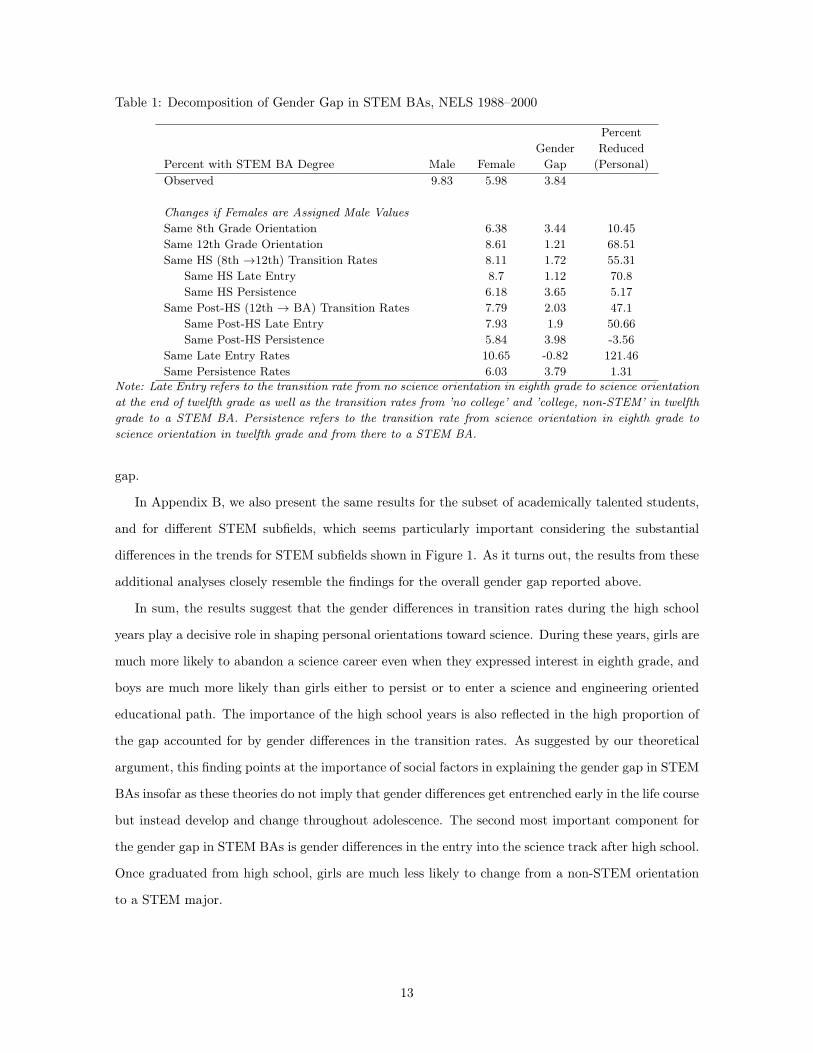
Table 1: Decomposition of Gender Gap in STEM BAs, NELS 1988–2000

Percent with STEM BA Degree Male FemaleGender

Gap

PercentReduced

(Personal)Observed 9.83 5.98 3.84

Changes if Females are Assigned Male Values

Same 8th Grade Orientation 6.38 3.44 10.45Same 12th Grade Orientation 8.61 1.21 68.51Same HS (8th →12th) Transition Rates 8.11 1.72 55.31

Same HS Late Entry 8.7 1.12 70.8Same HS Persistence 6.18 3.65 5.17

Same Post-HS (12th → BA) Transition Rates 7.79 2.03 47.1Same Post-HS Late Entry 7.93 1.9 50.66Same Post-HS Persistence 5.84 3.98 -3.56

Same Late Entry Rates 10.65 -0.82 121.46Same Persistence Rates 6.03 3.79 1.31

Note: Late Entry refers to the transition rate from no science orientation in eighth grade to science orientation

at the end of twelfth grade as well as the transition rates from ’no college’ and ’college, non-STEM’ in twelfth

grade to a STEM BA. Persistence refers to the transition rate from science orientation in eighth grade to

science orientation in twelfth grade and from there to a STEM BA.

gap.

In Appendix B, we also present the same results for the subset of academically talented students,

and for different STEM subfields, which seems particularly important considering the substantial

differences in the trends for STEM subfields shown in Figure 1. As it turns out, the results from these

additional analyses closely resemble the findings for the overall gender gap reported above.

In sum, the results suggest that the gender differences in transition rates during the high school

years play a decisive role in shaping personal orientations toward science. During these years, girls are

much more likely to abandon a science career even when they expressed interest in eighth grade, and

boys are much more likely than girls either to persist or to enter a science and engineering oriented

educational path. The importance of the high school years is also reflected in the high proportion of

the gap accounted for by gender differences in the transition rates. As suggested by our theoretical

argument, this finding points at the importance of social factors in explaining the gender gap in STEM

BAs insofar as these theories do not imply that gender differences get entrenched early in the life course

but instead develop and change throughout adolescence. The second most important component for

the gender gap in STEM BAs is gender differences in the entry into the science track after high school.

Once graduated from high school, girls are much less likely to change from a non-STEM orientation

to a STEM major.

13

The Role of High School for the Gender Gap

in STEM Orientation

The last section demonstrated our first central contention that the high school years play a crucial role

in shaping the orientation towards science and engineering among boys and girls. We now examine

the role of high school context for shaping orientations towards science and engineering during this

decisive period. In particular, we use multilevel models to document how the gender gap in STEM

orientation at the end of high school varies across high schools, and estimate the causal effect of the

high school curriculum on the gender gap in STEM orientation. For this purpose, we use two special

samples from the National Education Longitudinal Study. Compared to the 1988 to 2000 panel study

(NELS 88-2000), these two special samples only follow the students until their senior year in high

school, but they offer important advantages for our analytic goals. NELS 88-92 includes the full

eighth grade sample of NELS (~25,000), which is a much larger sample than NELS 88-20008, as well

as important pre-high school variables about the early science and engineering orientation. The NELS

88-92 sample does not, however, generally include a large number of students per high school because

eighth-grade students in the same school typically transitioned to more than one high school. The

NELS High School Effectiveness Study (HSES), which is the second dataset we use in the following

analysis, addresses this problem. As an independent component of NELS, the HSES extended the

sample of students in a subset of 250 high schools in the first follow-up 1990 so that these schools

had a sufficiently large number of students per school to support our analytic strategy. In contrast to

NELS 88-92, however, HSES does not include pre-high school information. The sample restrictions

for both datasets, the multiple imputation procedure used to recover missing data, and the variables

are described in Appendix A.

In the following analysis we use both NELS 88-92 and HSES to study the variation of the gender

gap across schools conditional on regional and urban variations. For this purpose, we specify a logistic

multilevel model that captures variation in the gender gap in twelfth grade STEM orientation across

schools. The outcome variable is the STEM orientation in twelfth grade at the end of high school. A

value of 0 indicates that a student does not intend to study a STEM field in college after graduating

from high school, whereas a value of 1 indicates that students intend to study a STEM field after high

school. The results from this analysis show substantial variation in the gender gap across high schools

even after controlling for a comprehensive set of pre-high school covariates. This finding, described in

more detail over the next paragraphs, indicates that the high school context plays an important role8Only a randomly selected subset of students were followed after high school.

14

Tabl

e2:

Var

iati

onof

Hig

hSc

hool

STE

MO

rien

tati

onac

ross

Scho

ols

NE

LSH

SES

NE

LSH

SES

NE

LS88

-92

NE

LS88

-92

NE

LS88

-92

Coe

f.(s

e)C

oef.

(se)

Coe

f.(s

e)C

oef.

(se)

Coe

f.(s

e)Fix

ed

Effects

Inte

rcep

t-2

.093

***

(0.0

6)-1

.991

***

(0.1

4)-1

.599

***

(0.0

3)-1

.719

***

(0.0

9)-2

.127

***

(0.1

0)Fe

mal

e-0

.906

***

(0.0

8)-0

.985

***

(0.0

9)-1

.109

***

(0.0

5)-1

.118

***

(0.0

6)-0

.897

***

(0.0

6)St

anda

rdD

emog

raph

icC

ontr

olV

aria

bles

yes

yes

yes

Reg

ion-

Urb

anC

ontr

olye

sye

sye

sP

re-H

igh

Scho

olC

ontr

olV

aria

bles

yes

Random

Effects

SDfo

rIn

terc

ept

0.54

80.

393

0.24

70.

243

0.27

5SD

for

Fem

ale

0.35

50.

424

0.42

30.

361

0.30

3Lo

g-Li

kelih

ood

Rat

ioC

hi-s

quar

e10

4.2*

**10

9.2*

**35

0.6*

**27

9.42

***

270.

62**

*P

-val

ue0.

000

0.00

00.

000

0.00

00.

000

Scho

ols

250

250

1,28

01,

280

1,28

0Av

g.St

uden

tspe

rSc

hool

37.1

37.1

10.2

10.2

10.2

Stud

ents

9,12

09,

120

13,6

4013

,640

13,6

40N

ote

:A

deta

iled

descrip

tion

ofth

econtrolvaria

ble

sis

inA

ppendix

Table

A1.

The

likelihood

ratio

chi-square

isa

testfo

rwheth

er

the

effectoffe

male

varie

sacross

hig

hschools.

*p

<0.0

5,**

p<

0.0

1,***

p<

0.0

01

15

in shaping the gender gap in STEM orientation.

We begin with a simple model that only includes female as an independent variable along with a

random intercept and a random slope at the school level that allows the effect of gender on high school

STEM orientation to vary across high schools. The results from this multilevel model fitted with the

HSES as well as the NELS 88-92 data are presented in Table 2. The estimated coefficients show a

substantial gender effect; the odds of reporting an intention to study a STEM field in college at the

end of high school for female are about 60% (HSES) or 70% (NELS 88-92) lower than the odds for

males (the female/male odds ratio are 0.4 and 0.3 as calculated from the coefficients on the log-odds

scale reported in the table). The results in the last section showed that this substantial gender gap at

the end of high school is decisive for the later gender gap in STEM bachelor degrees, accounting for

nearly 70% of the gap. The gender gap in personal STEM orientation, however, varies substantially

across high schools. Specifically, the estimated standard deviation of the random effect on the school

level implies that the gender gap ranges from 0.20 to 0.82 female/male odds ratios in the middle 95%

of schools (these are the more conservative estimates from a HSES dataset). In other words, the odds

for girls having a STEM interest are only 18% lower than the odds for boys in schools at one end of

this spectrum, whereas in schools at the other end the difference is 80%. This variation is illustrated

in Figure 5, which shows the distribution of the empirical Bayes estimates for the 250 high schools in

HSES and the 1,280 high school in NELS 88-92. The graph also illustrates the analytical limitations

of the NELS 88-92 dataset: Even though the estimated random slope for the variation of the gender

effect across schools is bigger in NELS 88-92 than in HSES, the empirical Bayes estimates do not vary

as strongly. The reason for this difference is the smaller average number of students per school in

NELS 88-92. Empirical Bayes estimates are so-called “shrinkage” estimates; they are a weighted sum

of the estimates from a single school and the estimates predicted for that school by data for the larger

population (which is the prior information from a Bayesian perspective). Empirical Bayes estimates

for schools with a large number of students put more weight on the school-specific estimate, while

empirical Bayes estimates for schools with a small number of students put more weight on the overall

gender gap so that their estimates are pulled more strongly towards the overall mean (for a discussion

of this see Gelman and Hill 2007). Despite considerable shrinkage towards the overall mean, the NELS

88-92 data do contain enough students per school to reveal substantial variation (from 0.3 to 0.45 for

the female/male odds ratio) in the gender slope across schools.

The revealed variation in the gender gap across schools might reflect the importance of the local

school context, but it is also possible that they arise from a non-random sorting of students into

different high schools such that girls with a strong science orientation are more likely to go to one

16

NELS HSES (without Control Variables)

Female/Male Odds-Ratio0.25 0.30 0.35 0.40 0.45 0.50 0.55 0.60

NELS 1988-1992 (without Control Variables)

Female/Male Odds-Ratio0.25 0.30 0.35 0.40 0.45 0.50 0.55 0.60

NELS 1988-1992(with Control Variables)

Female/Male Odds-Ratio0.25 0.30 0.35 0.40 0.45 0.50 0.55 0.60

Figure 5: Variation of Gender Gap in 12th Grade STEM Orientation across Schools, NELS 1988-92Note: The graph reports female/male odds-ratios so that a value of 1 indicates gender equality andvalues closer to one –i.e. higher values in this graph– a smaller gender gap.

school rather than another. In order to address this problem, we first add a number of standard

demographic measures and a categorical region-urban variable to both the HSES and the NELS 88-92

and then use the NELS 88-92 sample to also condition on a large number of eighth grade orientation

and performance measures (the variables are described in Appendix Table A1). We thereby obtain

an estimate of the high school effect on science and engineering orientation that is conditional on the

pre-high school science and math orientation as well as performance of students. The eighth grade

orientation measures include not only the expressed occupational plans of eighth grade students used in

the pathway analysis, but also four measures that assess whether middle school students like math and

science and whether they think that math and science is important for their future. The performance

measures are comprehensive and include three eighth grade test scores (math, science, and English),

and four GPA measures (math, science, English, and social studies). Because of this comprehensive

set of control variables for family background, region-urban, pre-high school science and engineering

orientation, and academic performance, these models can be understood as ’value-added’ models for

STEM orientation. Similar to value-added models in educational research on the effect of schools

and teachers on performance (e.g., Kane and Staiger 2008), the empirical Bayes estimates from these

models show the extent to which schools vary in supporting a science and engineering orientation

among high school students, conditional on their previous orientation. They also show the extent to

which schools are particularly supportive or unsupportive of a science orientation for girls net of the

school’s support for a science orientation for boys.

The results from these models are presented in Table 2 as well as Figure 5. They show that although

the estimated standard deviation for the school variation is smaller after pre-high school variables

are controlled, the remaining variation in the effect of the local environment is still substantial and

17

statistically significant. In particular, the estimated random slope from the multilevel model suggests

that the gender gap ranges from 0.22 to 0.75 female/male odds ratio in 95% of the schools. Figure 5

shows the distribution of the empirical Bayes estimates, which indicate substantial variations across

schools (the female/male odds ratio ranges from 0.34 to 0.50) despite the considerable pooling towards

the overall mean in the NELS 88-92 sample .

Overall, the results presented so far show substantial variation in the gender gap in science and

engineering orientation across schools. Net of science and math orientation in eighth grade, high

schools appear to play an important role in shaping these orientation among boys and girls. This

finding provides support for our argument that the local as well as the global environment shapes

the gender gap in orientation towards STEM fields. It remains unclear, however, which particular

characteristics of the high school explain these variations. In the remaining part of this section, we

begin to explore this question and also address two important follow-up questions.

The Effect of High School Curriculum on the Gender Gap in STEM Orien-

tation

The analyses so far have demonstrated the importance of the high school years for the persisting gender

gap in STEM degrees, and have shown substantial variation in the gender gap in STEM orientations

across high schools, net of pre-high school orientation. In this section, we estimate the causal effect

of the math and science curriculum in high school on the STEM orientation in twelfth grade for boys

and girls. This analysis helps us to understand the variations across the local school environment,

which is highly relevant from a policy perspective. Based on the theoretical argument developed

above, we would argue that a math and science orientation in high school as reflected in the course

offerings in math and science has a positive effect on the STEM orientation for both boys and girls,

and that the effect should be especially large for girls. We expect the strength of gender stereotypes

about occupations to vary inversely with the level of information about these careers provided by the

local environment, and about the relevance of gender to success in these careers. Given that girls

currently perform at the same level as boys in advanced math and science high school courses, we

expect that experiential knowledge of this fact and of the actual character of science and mathematics

– as revealed in advanced coursework – will weaken gender stereotypes and lead to a reduced gender

gap in STEM orientation during high school.

In order to estimate the causal effect of the math and science curriculum in high school, we

use the fact that the original NELS sample was first interviewed in eighth grade before students

18

attended high school. This feature of the data allows us to condition on the same comprehensive

set of pre-treatment variables used before. These variables are directly related to the selection of

students into high schools with a strong math and science curriculum. A number of recent studies

that compare experimental results with regression and matching estimates have shown that such a

comprehensive set of pre-treatment variables is essential to reduce the bias in estimates that are based

on regression or matching methods (Cook et al. 2009; Shadish et al. 2008). These studies also suggest

that the actual method used to estimate the effect – regressions based on the raw data or based on a

matched sample – plays a negligible role relative to the importance of the right pre-treatment controls

and despite the theoretical advantages of matching (for corroborating arguments, see Angrist and

Pischke 2008). Accordingly, the estimates presented below are based on logistic regressions using a

comprehensive set of pre-treatment control variables from eighth grade, including not only standard

demographic measures but also the eighth grade orientation towards math and science, the extent

to which a student reports that s/he likes math and science, and a set of seven GPA and test score

performance measures for reading, math and science (for a detailed description of the variables see

Appendix Table A1). The focal treatment variable is the intensity of the high school course offerings

in math and science. We measure this variable based on a set of questions asked in the tenth grade

school questionnaire about the courses offered at a school. In particular, we create an index based

on the AP or college or university level course offered for 31 different math and science areas such as

biology, physics, life science, calculus, and trigonometry, and we standardize this index with a mean

of zero and a standard devision of one. Appendix C contains a detailed description of the estimation

strategy, the sample, the variables and an assessment of the balance between different levels of the

treatment indicator.

Table 3 presents estimates of a STEM orientation at the end of high school from logistic regressions

on the curriculum index for boys and girls conditional on a large set of pre-treatment covariates. The

table shows separate estimates for students who did not indicate a science orientation in eighth grade

and for those who did. Accordingly, the table shows both estimates for the probability of late entry

into the science track during high school as well as for the probability of persistence in the science

track during high school. Our prior analysis revealed a substantial gender gap in both the late entry

and the persistence rate, but also indicated that the difference in male and female rates of late entry

by gender (which can be understood as the ability of a high school to recruit boys and girls into the

science track) plays a decisive role in gender gap in STEM degrees. The results for late entry in table

3 show a substantial gender gap in the late entry rate as previously observed. In particular, boys are

2.3 times as likely as girls to transfer into a science track during high school (male/female odds ratio).

19

Tabl

e3:

Logi

stic

Reg

ress

ion

Est

imat

esof

STE

MO

rien

tati

onin

12th

Gra

deon

Hig

hSc

hool

Mat

han

dSc

ienc

eC

urri

culu

m

Late

Ent

ryLa

teE

ntry

Late

Ent

ryPer

sist

ence

Per

sist

ence

Per

sist

ence

Coe

f(s

e)C

oef

(se)

Coe

f(s

e)C

oef

(se)

Coe

f(s

e)C

oef

(se)

Inte

rcep

t-2

.760

***

(0.0

5)-2

.824

***

(0.0

6)-3

.056

***

(0.0

9)-0

.984

***

(0.1

4)-1

.036

***

(0.1

6)-1

.676

***

(0.2

3)C

urri

culu

mIn

dex

(CI)

0.13

6**

(0.0

5)0.

138*

*(0

.05)

0.11

1*(0

.06)

-0.1

03(0

.17)

-0.1

02(0

.17)

-0.0

50(0

.19)

Mal

e1.

027*

**(0

.07)

1.07

6***

(0.0

7)0.

839*

**(0

.08)

0.45

3**

(0.1

6)0.

492*

*(0

.16)

0.39

8(0

.21)

Cur

ricu

lum

Inde

x(C

I)x

Mal

e-0

.140

*(0

.06)

-0.1

47*

(0.0

7)-0

.163

*(0

.07)

0.08

5(0

.18)

0.08

9(0

.19)

-0.0

33(0

.20)

Stan

dard

Dem

ogra

phic

Con

trol

Var

iabl

esye

sye

sye

sye

sA

ddit

iona

lCon

trol

Var

iabl

esye

sye

sye

sye

sP

re-H

igh

Scho

olC

ontr

olV

aria

bles

yes

yes

Stud

ents

12,2

7012

,270

12,2

7091

091

091

0N

ote

:C

ontrolvaria

ble

sare

describ

ed

inA

ppendix

Table

A1.

*p

<0.0

5,**

p<

0.0

1,***

p<

0.0

01

20

-1.0 -0.5 0.0 0.5 1.0

1.5

2.0

2.5

3.0

Math and Science Curriculum (Index)

Mal

e/Fe

mal

e O

dds-

Rat

io

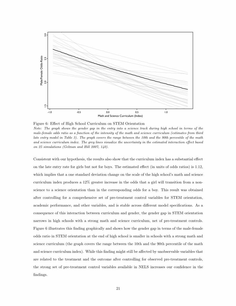
Figure 6: Effect of High School Curriculum on STEM OrientationNote: The graph shows the gender gap in the entry into a science track during high school in terms of the

male-female odds ratio as a function of the intensity of the math and science curriculum (estimates from third

late entry model in Table 3). The graph covers the range between the 10th and the 90th percentile of the math

and science curriculum index. The grey lines visualize the uncertainty in the estimated interaction effect based

on 25 simulations (Gelman and Hill 2007, 140).

Consistent with our hypothesis, the results also show that the curriculum index has a substantial effect

on the late entry rate for girls but not for boys. The estimated effect (in units of odds ratios) is 1.12,

which implies that a one standard deviation change on the scale of the high school’s math and science

curriculum index produces a 12% greater increase in the odds that a girl will transition from a non-

science to a science orientation than in the corresponding odds for a boy. This result was obtained

after controlling for a comprehensive set of pre-treatment control variables for STEM orientation,

academic performance, and other variables, and is stable across different model specifications. As a

consequence of this interaction between curriculum and gender, the gender gap in STEM orientation

narrows in high schools with a strong math and science curriculum, net of pre-treatment controls.

Figure 6 illustrates this finding graphically and shows how the gender gap in terms of the male-female

odds ratio in STEM orientation at the end of high school is smaller in schools with a strong math and

science curriculum (the graph covers the range between the 10th and the 90th percentile of the math

and science curriculum index). While this finding might still be affected by unobservable variables that

are related to the treatment and the outcome after controlling for observed pre-treatment controls,

the strong set of pre-treatment control variables available in NELS increases our confidence in the

findings.

21

The logistic regression results for persistence, however, do not show a gender difference in the effect

of the math and science curriculum. The estimated effect is both substantially smaller and statistically

insignificant, which implies that the high school math and science curriculum mainly works through

its power to recruit girls into science and engineering and not through its power to retain girls in

science who have previously reported a STEM orientation. This pattern of results is consistent with

the findings from our pathways model. The gender gap in STEM BAs is not primarily a consequence

of girls losing their personal STEM orientation at a greater rate than boys, but rather from the lower

rate of recruitment of girls into a STEM orientation between eighth grade and the senior year of

college.

Is the High School Effect Lasting?

A common argument in the debate on the the effect of teachers on the learning of students is that

potential gains in performance abate over the following years (Rothstein 2010; Jacob et al. 2010). A

similar concern should apply to the effect of high school on the science and engineering orientation of

boys and girls. If girls who were enrolled in high schools that were especially good recruiters of girls

into a personal STEM orientation were to leak from the science pipeline at higher rates, the school

effect would not be an important determinant of the gender gap in STEM bachelors degrees. In a

recent review of interventions to increase female interest in science and technology (e.g., Turner and

Lapan 2005; Plant et al. 2009), Hill et al. (2010) noted the uncertainty about the long term effects

of these interventions that arises simply from the lack of long-term followup data. In this respect,

the NELS data are attractive because they allow a direct assessment of the durability of high school

effects on STEM orientations.

In order to conduct this assessment, we group high schools by the size of the gender gap in science

and engineering orientation and examine the post-high school transition rates used in the pathway

analysis above. In particular, we use the empirical Bayes estimates of the gender gap from the ’value-

added’ multilevel model (NELS 88-92) above to group schools into those with a small gender gap

(bottom terciles) and those with a big gender gap (top terciles). We then match this newly created

school-level variable to the students in NELS 88-2000 and calculate the post-high school transition

rates separately for the full school sample (already shown in the graphs above) as well as the high

schools with a small and big gender gap.

Table 4 presents the results from this analysis. It shows that the post-high school transition rates

are remarkably constant across the three samples. Neither of the transition rates differs significantly

22

Table 4: Post-High School Transition Rates for Full Sample, and School with Small/Big Gender Gap

Post-HS TransitionRates

Gender Full Sample Schools with SmallGender Gap

Schools with BigGender Gap

Leakage Rate male 0.669 0.615 0.692female 0.649 0.686 0.637

Late Entry Rate male 0.078 0.084 0.082female 0.051 0.06 0.039

Persistence Rate male 0.331 0.385 0.308female 0.351 0.314 0.363

Note: Late Entry refers to late entry from a college but non-STEM orientation at the end of high school.

between the three samples. Accordingly, students from high schools that encourage a science and

engineering orientation among women do not have higher leakage rates from the science pipeline than

their peers from schools with a big gender gap. This finding suggests that the effect of high schools

on the science and engineering orientation of women is not temporary, but instead endures after high

school and ultimately reduces the gender gap in the attainment of STEM BAs. Accordingly, high

schools seem to be an effective agent for policy initiatives to reduce the gender gap in STEM degrees.

How Much does the High School Effect Matter?

Building on the findings from the last section, we ask how much the gender gap would be reduced

if all schools would encourage women to study science and engineering at the same rate as schools

in the bottom tercile of the gender gap. For this purpose, we again group high schools into terciles

according to the size of their gender gap in STEM orientation. We then calculate the gender gap in

STEM BA degrees assuming the same eighth grade orientation and post-high school transition rates

across all three samples. In other words, we assume that differences in the gender gap across the

three samples only emerge because of differences in the transition rates within high school, and not

from group differences in eighth grade orientation and transition rates after high school. As shown in

Table 5, boys are 1.7 times as likely as girls to graduate from college with a STEM BA degree in the

entire sample. However, this substantial male advantage is reduced to 1.3 (male/female odds ratio)

in the sub-sample of students who attend high schools with a small gender gap. Accordingly, the

gender gap would be reduced by about 25% if the environment in all schools would encourage girls

to study science and engineering at the same rates as the top third of schools. The reduction would

presumably be even larger if all schools could achieve the same results as the most gender-egalitarian

schools in our sample.

23

Table 5: Gender Gap in STEM BAs for Full Sample, Schools with Small Gender Gap, and Schoolswith Big Gender Gap

Proportion of Students with Gender GapSTEM bachelor degree Male Female in % Odds RatioFull Sample 0.098 0.060 0.038 1.713Schools with Small Gender Gap 0.124 0.095 0.029 1.349Schools with Big Gender Gap 0.077 0.039 0.039 2.089

Conclusion

Despite the striking reversal of the gender gap in educational attainment and the near gender parity

in math performance, women still pursue science, technology, engineering, and math degrees at much

lower rates than their male peers do. In this paper, we have explored two important and related

dimensions of this persisting gender gap in STEM degrees: First, the timing in the emergence of

the gender gap in orientation towards STEM fields, and second, variations in the gender gap across

high schools. Based on an examination of biological, psychological, and sociological theories about

gender, we have argued that the process of forming gender stereotypes unfolds throughout adolescence,

and that the local high school environment plays an important role in shaping the gender gap. We

then turned to an empirical examination of the two dimensions. First, we decomposed the gender

gap in STEM bachelor degrees into various pathways to examine the emergence and solidification of

gender differences in the orientation towards science and engineering in the adolescent life course. In

particular, we used the National Education Longitudinal Study to follow the 1988 cohort of eighth

grade students through adolescence and young adulthood, and we observed how orientations towards

STEM fields emerge and change during these years. Our findings show that the substantial gender gap

in eighth grade orientation is relatively inconsequential for the persisting gender gap in STEM degrees

at the completion of college. Instead, the high school years play a major role in shaping gendered

orientations towards science and engineering. Second, we used multilevel models to examine how the

gender gap in STEM orientation at the end of high school varies across schools, net of pre-treatment

controls. The results show substantial variation in the gender gap in STEM orientation across schools,

and support our argument that the local environment plays a major role in shaping and gendering

orientations towards education and career among boys and girls. Our additional analyses show that

this high school effect seems to be related to the math and science orientation of the school.

Existing theories of the persisting gender gap in STEM degrees focus on gender differences in

mathematical ability as well as women’s lack of interest in STEM degrees, and point at biological,

psychological, and sociological theories to explain these differences. While the analyses conducted in

24

this paper are not designed to provide a definitive test for any of the theories, the results nonetheless

have important implications for the existing debate. Our findings identify adolescence as the crucial

period in life when the gender gap in orientations towards STEM fields solidifies at the individual

level. They argue against gender essentialist theories and instead support theoretical accounts for

gender segregation in science and mathematics fields of study that emphasize the importance of

the local environment in shaping the gender gap in STEM degrees. These include social-cognitive

theories from psychology, and sociological theories which emphasize local environmental influence on

the construction and salience of gender stereotypes, status expectations, and career aspirations. In this

respect, our results parallel recent research which shows that academically-oriented classroom and peer

cultures in late elementary school have especially strong effects on the academic performance of boys

(Legewie and DiPrete 2011). Legewie and DiPrete’s results suggested that learning-oriented academic

climates in school counteract masculine stereotypes that favor an oppositional attitude towards school

and thereby undermine the educational performance of boys. In both that study and the current

one, greater investment in the school climate works to mitigate the negative consequences of gender

stereotypes (in one case involving females and the other case involving males) that undermine the

educational process.

Not all local environmental effects are necessarily durable, of course. Indeed, recent research on

social-psychological interventions in education to counter racial or gender stereotypes have triggered

an active debate about whether the effects in question are real, scalable, or long-lasting (Yeager and

Walton 2011). High school context is, of course, a much more intensive and extensive “treatment”

than are the targeted interventions found in the social-psychological literature on stereotype threat.

However, in light of recent research asserting only a temporary effect from exposure to Head Start

programs or to individual above-average teachers (Jacob et al. 2010), it is of considerable importance

that the effects of the high school environment on the formation of STEM orientations appear to be

durable. Our findings, therefore, have important policy implications. The pathway analysis shows

that high school is the decisive life period during which the gender gap emerges, and the examination

of variations across contexts shows that the local context in high school plays an important role for the

gender gap in orientations towards STEM fields. As such, our findings not only point at the life course

period that should be targeted by policy interventions, but also provide evidence that high school

interventions might be effective. Some existing interventions have targeted high school students and

shown success in promoting a STEM orientation among girls. Eisenhart (2008), for example, discusses

a seemingly effective outreach project that educates high-achieving, minority girls in high school about

science and engineering jobs. While such policy interventions have to withstand the serious scrutiny of

25

experimental field trials, the evidence presented in this paper encourages researchers and policy makers

alike to take seriously the potential impact of high school interventions on the STEM orientations of

female students. Our finding that the intensity of the math and science curriculum reduces the gender

gap in science orientation strongly supports this conclusion.

The present study obviously falls short in adequately addressing all the characteristics of high

schools that influence the gender gap. Similar to the state of knowledge about teacher quality, our

findings suggest that high schools have the potential to shape the orientation towards STEM fields

and suggest that the math and science orientation of the school might play an important role, but we

still know relatively little about other high school characteristics or programs that achieve this goal.

Our own theoretical argument suggests that the ways in which gender identities are constructed plays

an important role. Our argument also suggests that commonly held stereotypes are strengthened by

the lack of adequate information about science and engineering careers in the local environment, and

conversely that the power of these stereotypes over behavior can be reduced through greater exposure

to knowledge about science and engineering through the academic curriculum. A third argument was

presented recently by Frank et al. (2008), who argue that social dynamics play an important role for

the propensity of girls and boys to take math courses. Future research should investigate these issues

at greater depth in order to extend our knowledge about the persisting gender gap in STEM degrees.

26

Appendix A Samples, Variables, and Missing Data

The analyses presented in this paper are based on three samples from the National Education Longitu-

dinal Study of 1988 (NELS). NELS is a nationally representative sample of about 25,000 eighth grade

students who were first surveyed in the spring of 1988. Subsamples of these students were resurveyed

in 1990, 1992, 1994, and 2000 so that the students were followed over time as they graduated from

high school and entered the labor force or pursued post-secondary degrees. The panel structure of

the data combined with the fact that it includes detailed information on educational careers allows

us to examine the different questions addressed in this paper. We have briefly described each of the

three samples in the main text and provide further details in this appendix. Table A1 also contains a

detailed description of the variables used in the different analyses.

NELS 1988-2000 Sample (Pathway Analysis) We restrict the NELS 88-2000 sample to students

who participated in the eighth and 12 grade survey (base year and second follow up), the 2000

follow up (fourth follow up).9 The size of this restricted sample is 8,320. From this sample,

1,260 (15.2%) cases are dropped because of missing data on the relevant variables, which brings

the analysis sample down to 7,060. All of the analysis use the appropriate weights provided by

NELS.

NELS 1988-1992 Sample (High School Context Analysis) We restrict our analysis of the NELS

88-1992 to students who participated in the base year as well as the first and second follow up

and to those for which the school filled out a school questionnaire during the first follow up. The

size of this sample is 13,640.10 5,310 or 38.9% of these cases have missing data on at least one

of the large number of pre-treatment control or other variables. To address this problem, we use

multiple imputations based on the multivariate normal model approach with a large number of

auxiliary variables such as 10th and 12th grade test scores in reading, math and science.

NELS HSES Sample (High School Context Analysis) The HSES sample used in our analysis

contains all 9,740 students who participated in the twelfth grade survey. 1,720 or 17.63% of the

students have missing data on at least one of the variables. Similar to our analysis based on the

NELS 1988-1992, we use multiple imputations to recover cases with missing data.9This sample restriction excludes high school drop-outs. Although NELS followed students who dropped out of high

school, information on intentions to go to college are meaningless so that it makes sense to exclude this group from ouranalysis.

10For the estimation of the curriculum effect we also exclude students who did not change school between eighth andtenth grade and those who changed school between tenth and twelfth grade. Accordingly, the analysis of the curriculumeffect is based on students who changed from a middle to a high school and proceeded to 12th grade without droppingout of school or changing the school. This restriction excludes 450 cases.

27

Table A1: Description of Variables

Variables Description

STEM Orientation in School and STEM Bachelor Degree Attainment8th Grade STEM Orientation Binary indictor based on occupational aspiration in eighth grade (“What

kind of work do you expect to be doing when you are 30 years old?”):0=not science or engineering (12 categories such as craftsperson,housewife, business owner and others);1=“science or engineering professional, such as engineer or scientist”

12th Grade STEM Orientation Our coding first uses the filter question “Do you plan to continue youreducation past high school at some time in the future?” to determine thepeople who do not plan to go to college. We then use the intended fieldof study question to distinguish between STEM fields (science,technology, engineering, or mathematics) or non-STEM fields.Pathway analysis:1=no college2=College, no STEM field3=College, STEM field

MLM and curriculum effect:0=no college or college but no STEM1=College, STEM field

STEM bachelor Attainment of bachelor degree from a four year college in a STEM fielduntil 2000 (eights years after the normal high school graduation). STEMfield was recoded based on the Classification of Instructional Programs(CIP) and is defined as any degree in science, technology, engineering, ormathematics.

Demographic Control Variables (NELS 88-1992 and NELS HSES)

Gender 0 - Female; 1 - MaleRace Categorical (reference category is White): Asian, Hispanic, Black (not

Hispanic), White (not Hispanic), Native AmericanAge continuos (standardized)Family Status Standardized socio-economic status composite constructed from father’s

education level, mother’s education level, father’s occupation, mother’soccupation, and family income (from eighth grade data for NELS88-2000 and 88-1992, and from 10th and 12th grade for NELS HSES)

Pre-High School Control Variables (NELS 88-1992)

Performance (Test Scores) eighth grade reading, math, and science test scores (separate, ctsvariables)

Performance (GPA) Self reported English, math, science, and social studies grades from 6thto 8th grade (separate, cts variables)

8th Grade Science Orientation see aboveMath/Science Interest “I usually look forward to mathematics class”

“I usually look forward to science class” (four point Likert scale, 8thgrade)

Math/Science Usefulness “Math will be useful in my future”“Science will be useful in my future” (four point Likert scale, 8th grade)

Math/Science Extra Curricular Three dichotomous indicators (8th grade) for participation in math club,science club, and science fair.

Additional Control Variables (NELS 88-1992 and NELS HSES)

Region-Urban Categorical variable with twelve groups defined by all the possiblecombination of four large US regions (Northeast, North Central, South,West) and the urbanicity of the area (urban, suburban, and rural).

Note: All continuos variables have been standardized for the analysis.

28

Appendix B Pathways for Academically Talented Students and

Different STEM Subfields

In this appendix, we present the findings from the pathway analysis for academically talented students,

and for different STEM subfields. Academically talented students are defined in terms of their math

performance in eighth grade. Restricting the sample to the top 33% students in terms of math

performance leads to similar results but the patterns reported above are even more pronounced (see

Table A2). The transition rates during high school play an ever bigger role (64.1% compared to

55.3%) and the different rates of late entry after high school a slightly smaller role (44.9% compared

to 50.7%).

The trends presented in Figure 1 suggest that analyzing gender differences in STEM degrees should

take into account the substantial differences between sub-fields. Accordingly, we analyze engineering,

math and physics as well as bio/life-science respectively and look at how the pathways for these sub-

fields differ from STEM fields in general. Table A2 presents the results of these decompositions. For

both engineering as well as math and physics, the results resemble the findings from STEM fields

in general. In all three cases, the transition rates in high school play the most important role in

explaining gender differences in an engineering BA, while the lower rate of late entry for females after

high school plays the second most important role. For biology and life science, the gender gap in

bachelor degrees is small and not statistically significant, and therefore a decomposition analysis is

not informative.

Appendix C Estimating the Effect of High School Curriculum

on the Gender Gap in STEM Orientation

The literature on the estimation of causal effect using conditioning on observable covariates as an

identification strategy has recently focused on matching procedures. Theoretically, estimates based

on matched samples provide a number of advantages over regression estimates based on the raw data.

Most notably, matching estimates are (quasi) non-parametric, and reduce the need to extrapolate by

discarding (or down-weighting) observations without common support in the treatment and control

group. A number of recent studies that compare experimental with regression and matching estimates,

however, have shown that these theoretical advantages are typically negligible in practice (Cook et al.

2009; Shadish et al. 2008; Angrist and Pischke 2008). These studies instead point at the importance

29

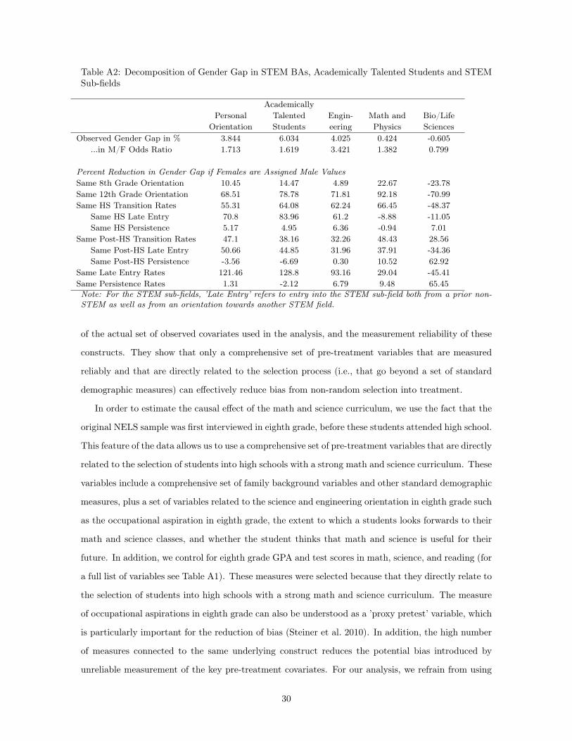
Table A2: Decomposition of Gender Gap in STEM BAs, Academically Talented Students and STEMSub-fields

PersonalOrientation

AcademicallyTalentedStudents

Engin-eering

Math andPhysics

Bio/LifeSciences

Observed Gender Gap in % 3.844 6.034 4.025 0.424 -0.605...in M/F Odds Ratio 1.713 1.619 3.421 1.382 0.799

Percent Reduction in Gender Gap if Females are Assigned Male Values

Same 8th Grade Orientation 10.45 14.47 4.89 22.67 -23.78Same 12th Grade Orientation 68.51 78.78 71.81 92.18 -70.99Same HS Transition Rates 55.31 64.08 62.24 66.45 -48.37

Same HS Late Entry 70.8 83.96 61.2 -8.88 -11.05Same HS Persistence 5.17 4.95 6.36 -0.94 7.01

Same Post-HS Transition Rates 47.1 38.16 32.26 48.43 28.56Same Post-HS Late Entry 50.66 44.85 31.96 37.91 -34.36Same Post-HS Persistence -3.56 -6.69 0.30 10.52 62.92

Same Late Entry Rates 121.46 128.8 93.16 29.04 -45.41Same Persistence Rates 1.31 -2.12 6.79 9.48 65.45Note: For the STEM sub-fields, ’Late Entry’ refers to entry into the STEM sub-field both from a prior non-

STEM as well as from an orientation towards another STEM field.

of the actual set of observed covariates used in the analysis, and the measurement reliability of these

constructs. They show that only a comprehensive set of pre-treatment variables that are measured

reliably and that are directly related to the selection process (i.e., that go beyond a set of standard

demographic measures) can effectively reduce bias from non-random selection into treatment.

In order to estimate the causal effect of the math and science curriculum, we use the fact that the

original NELS sample was first interviewed in eighth grade, before these students attended high school.

This feature of the data allows us to use a comprehensive set of pre-treatment variables that are directly

related to the selection of students into high schools with a strong math and science curriculum. These

variables include a comprehensive set of family background variables and other standard demographic

measures, plus a set of variables related to the science and engineering orientation in eighth grade such

as the occupational aspiration in eighth grade, the extent to which a students looks forwards to their

math and science classes, and whether the student thinks that math and science is useful for their

future. In addition, we control for eighth grade GPA and test scores in math, science, and reading (for

a full list of variables see Table A1). These measures were selected because that they directly relate to

the selection of students into high schools with a strong math and science curriculum. The measure

of occupational aspirations in eighth grade can also be understood as a ’proxy pretest’ variable, which

is particularly important for the reduction of bias (Steiner et al. 2010). In addition, the high number

of measures connected to the same underlying construct reduces the potential bias introduced by

unreliable measurement of the key pre-treatment covariates. For our analysis, we refrain from using

30

Figure A1: Balance between Top and Bottom Quartile of Continuos Treatment Variable

-0.4 -0.2 0.0 0.2 0.4

0.0

0.5

1.0

1.5

2.0

2.5

(a) Balance in Raw Data

Std. Difference in Means

Var

ianc

e R

atio

Rubin's Threshold

-0.4 -0.2 0.0 0.2 0.4

0.0

0.5

1.0

1.5

2.0

2.5

(a) Balance Conditional on Covariates

Std. Difference in Means

Var

ianc

e R

atio

Rubin's Threshold

Race: Native A. Race: Asian

matching procedures because of the common finding that regression and matching based estimates are

equally good and because our treatment measure is continuous. Dichotomizing the treatment indicator

would be a possibility but we believe that the gains from estimates based on matched samples (if any)

are offset by the precision lost introduced through dichotomizing the treatment indicator. To further

address this issue, we analyze the balance of the data across different values of the treatment indicator

below, and explore alternative model specifications to maximize balance.

The Treatment Indicator Our focal treatment variable is the intensity of the high school course

offerings in math and science. We measure this variable based on a set of questions asked in the tenth

grade school questionnaire about the courses offered at a school. In particular, we create an index

based on the AP or college or university level course offered for 31 different math and science areas

such as biology, physics, life science, calculus, and trigonometry, and standardize this index with a

mean of zero and a standard devision of one.

Balance between Levels of the Treatment Indicator To examine the balance between different

levels of the treatment indicator, we compare the first and fourth quartile of the treatment indicator

with respect to forty pre-treatment covariates in the raw data as well as conditional on the control

variables. These covariates include the control variables used in the final analysis but also a number

of interaction terms between these variables that are not included in the final analysis. Figure A1

shows balance in terms of the standardized difference in means (x-axis) and the variance ratio (y-axis)

for the raw data as well as conditional on the covariates in the final analysis. Solid circles indicate

key variables such as eighth grade orientation, and math and science performance. These variables

31

were selected based on theoretical considerations as well as the size of there effect in the selection and

outcome model. The grey rectangle indicates Rubin’s (2001) rule of the thumb, which suggests that

the absolute standardized differences in means should not be greater than 0.25 and the variance ratio

should be between 0.5 and 2. In general, however, imbalance should be reduced without limit. The

results show that the covariates clearly increase the balance between the treatment and control group

and that the highly relevant variables cluster right around the point of no imbalance. The only variable

that falls outside the rectangle is the dummy variable for Native Americans. This group, however, is

extremely small with only 30 students in the control group and 20 in the treatment group. Overall, the

results indicate that our estimation strategy is effective in reducing the observable imbalance between

different levels of the treatment indicator. Alternative specifications did not reduce the imbalance

further.

32

References

Adelman, Clifford. 2006. “The Toolbox Revisited. Paths to Degree Completion from High School

Through College.” Technical report, U.S. Department of Education.

Almquist, E.M., S.S. Angrist, and R. Mickelsen. 1980. “Women’s Career Aspirations and Achieve-

ments: College and Seven Years After.” Work and Occupations 7:367–384.

an Ghaill, Mairtin Mac. 1994. The Making of Men: Masculinities, Sexualities and Schooling . Buck-

ingham: Open University Press.

Andreescu, T., J. A Gallian, J. M Kane, and J. E Mertz. 2008. “Cross-cultural analysis of students

with exceptional talent in mathematical problem solving.” Notices of the AMS 55:1248–1260.

Angrist, Joshua D and Jorn-Steffen Pischke. 2008. Mostly Harmless Econometrics: An Empiricist’s

Companion. Princeton University Press.

Angrist, S.S. and E.M. Almquist. 1993. “The Carnegie Mellon Class of 1968: Families, careers, and

contingencies.” In Women’s Lives through Time: Educated American Women of the Twentieth

Century , edited by K.D. Hulbert and D.T. Schuster. San Francisco: Jossey-Bass.

Arnold, K.D. 1995. Lives of Promise: What becomes of High School Valedictorians. San Francisco:

Jossey-Bass.

Aronson, J. and C. M Steele. 2005. “Stereotypes and the fragility of academic competence, motivation,

and self-concept.” Handbook of competence and motivation p. 436–456.

Beutel, A.M. and M. Mooney Marini. 1995. “Gender and values.” American sociological review

60:436–448.

Buchmann, Claudia and Thomas A. DiPrete. 2006. “The Growing Female Advantage in College

Completion: The Role of Family Background and Academic Achievement.” American Sociological

Review 71:515–541.

Bussey, Kay and Albert Bandura. 1999. “Social cognitive theory of gender development and differen-

tiation.” Psychological Review 106:676–713.

Carrell, S. E, M. E Page, and J. E West. 2010. “Sex and Science: How Professor Gender Perpetuates

the Gender Gap*.” Quarterly Journal of Economics 125:1101–1144.

33

Ceci, S. J, W. M Williams, and S. M Barnett. 2009. “Women’s underrepresentation in science: Socio-

cultural and biological considerations.” Psychological Bulletin 135:218.

Charles, M. and K. Bradley. 2002. “Equal but separate? A cross-national study of sex segregation in

higher education.” American Sociological Review 67:573–599.

Coleman, James. 1966. Equality of educational opportunity . U.S. Dept. of Health, Education, and

Welfare, Office of Education.

Cook, Thomas D, Peter M. Steiner, and Steffi Pohl. 2009. “How Bias Reduction Is Affected by

Covariate Choice, Unreliability, and Mode of Data Analysis: Results From Two Types of Within-

Study Comparisons.” Multivariate Behavioral Research 44:828–847.

Correll, S.J. 2001. “Gender and the Career Choice Process: The Role of Biased Self-Assessments 1.”

American Journal of Sociology 106:1691–1730.

Correll, Shelley J. 2004. “Constraints into Preferences: Gender, Status, and Emerging Career Aspira-

tions.” American Sociological Review 69:93–113.

Davies, S. and N. Guppy. 1996. “Fields of Study, College Selectivity, and Student Inequalities in

Higher Education.” Social Forces 75:1439–1462.

DiPrete, Thomas and Anne McDaniel. 2011. “Family, Gender, and Educational Outcomes in Elemen-

tary and Middle School.” Paper Presented at the Population Association of America meetings in

Washington, D.C.

Duxbury, L.E. and C.A. Higgins. 1991. “Gender differences in work-family conflict.” Journal of Applied

Psychology 76:60–74.

Eccles, J.S. 2007. “Where are all the women? Gender differences in participation in physical science

and engineering.” In Why Aren’t More Women in Science? Top Researchers Debate the Evidence,

edited by S. J. Ceci and W. M. Williams. Washington, D.C.: American Psychological Association.

Eccles, JS and LW Hoffman. 1984. “Sex roles, socialization, and occupational behavior.” Child

development research and social policy 1:367–420.

Eccles, J. S. 1994. “Understanding women’s educational and occupational choices.” Psychology of

Women Quarterly 18:585–609.

Eisenhart, M. 2008. “We can’t get there from here: High school girls consider engineering.”

34

Ellison, G. and A. Swanson. 2010. “The Gender Gap in Secondary School Mathematics at High

Achievement Levels: Evidence from the American Mathematics Competitions.” The Journal of

Economic Perspectives 24:109–128.

England, P. 2005. “Gender inequality in labor markets: The role of motherhood and segregation.”

Social Politics: International Studies in Gender, State & Society 12:264.

Felmlee, D.H. 1993. “The Dynamic Interdependence of Women’s Employment and Fertility.” Social

Science Research 22:333–360.

Francis, Becky. 2000. Boys, Girls and Achievement: Addressing the Classroom Issues. Routledge

Falmer, 1 edition.

Frank, Kenneth A., Chandra Muller, Kathryn S. Schiller, Catherine Riegle-Crumb, Anna Strass-

mann Mueller, Robert Crosnoe, and Jennifer Pearson. 2008. “The Social Dynamics of Mathematics

Coursetaking in High School.” American Journal of Sociology 113:1645–1696.

Gelman, Andrew and Jennifer Hill. 2007. Data Analysis Using Regression and Multilevel/Hierarchical

Models. Cambridge: Cambridge University Press.

Gerson, K. 1985. Hard Choices: How Women Decide about Work, Career, and Motherhood . University

of California Press.

Good, C., J. Aronson, and J. A Harder. 2008. “Problems in the pipeline: Stereotype threat and

women’s achievement in high-level math courses.” Journal of Applied Developmental Psychology

29:17–28.

Guiso, Luigi, Ferdinando Monte, Paola Sapienza, and Luigi Zingales. 2008. “Culture, Gender, and

Math.” Science 320:1164–1165.

Habashi, M. M, W. G Graziano, D. Evangelou, and I. Ngambeki. 2009. “Teacher Influences on Child

Interest in STEM Careers.” In Proceedings of the Research in Engineering Education Symposium,

Palm Cove, QLD.

Halpern, D. F. 2000. Sex Differences in Cognitive Abilities . Mahwah, NJ: Lawrence Erlbaum Asso-

ciates.

Hauser, R. M, S. L Tsai, and W. H Sewell. 1983. “A model of stratification with response error in

social and psychological variables.” Sociology of Education 56:20–46.

35

Hedges, LV and A. Nowell. 1995. “Sex differences in mental test scores, variability, and numbers of

high-scoring individuals.” Science 269:41–45.

Hill, Catherine, Christianne Corbett, and Andresse St. Rose. 2010. Why So Few? Women in Science,

Technology, Engineering, and Mathematics. Washington, DC: American Association of University

Women.

Hyde, J.S., S.M. Lindberg, Linn M.C., Ellis A.B., and Williams C.C. 2008. “Gender Similarities

Characterize Math Performance.” Science 321:494–495.

Jacob, B. A, L. Lefgren, and D. P Sims. 2010. “The persistence of teacher-induced learning.” Journal

of Human Resources 45:915—943.

Jacobs, J. E and M. M Bleeker. 2004. “Girls’ and boys’ developing interests in math and science: Do

parents matter?” New Directions for Child and Adolescent Development 2004:5–21.

Jacobs, J. E, S. Lanza, D. W Osgood, J. S Eccles, and A. Wigfield. 2002. “Changes in children’s self-

competence and values: Gender and domain differences across grades one through twelve.” Child

Development 73:509–527.

Johnson, M.K. 2001. “Social Orgins, Adolescent Experiences, and Work Value Trajectories during the

Transition to Adulthood.” Social Forces 80:1307–1340.

Kane, T. J and D. O Staiger. 2008. Estimating teacher impacts on student achievement: An experi-

mental evaluation. National Bureau of Economic Research Cambridge, Mass., USA.

Kimura, D. 2002. “Sex hormones influence human cognitive pattern.” Neuroendocrinology Letters

23:67–77.

Konrad, A.M., J. E. Ritchie, P. Lieb, and E. Corrigall. 2000. “Sex differences and similarities in job

attribute preferences: A meta-analysis.” Psychological bulletin 126:593–641.

Lapan, Richard T., Angela Adams, Sherri Turner, and Jeanne M. Hinkelman. 2000. “Seventh graders’

vocational interest and efficacy expectation patterns.” Journal of Career Development 26:215–229.

Lee, J., W. Grigg, and G. Dion. 2007. The nation’s report card: Mathematics 2007 . Washington,

DC: National Center for Education Statistics, Institute of Education Sciences, US Department of

Education.

Legewie, Joscha and Thomas A. DiPrete. 2011. “School Context and the Gender Gap in Educational

Achievement.” American Sociological Review (forthcoming).

36

Liben, L. S, R. S Bigler, and H. R Krogh. 2001. “Pink and Blue Collar Jobs: Children’s Judgments

of Job Status and Job Aspirations in Relation to Sex of Worker* 1.” Journal of Experimental Child

Psychology 79:346–363.

Lippa, Richard A. 2005. Gender, Nature, and Nurture. Psychology Press, 2 edition.

Lohman, David F. and Joni M. Lakin. 2009. “Consistencies in sex differences on the cognitive abilities

test across countries, grades, test forms, and cohorts.” British Journal of Educational Psychology

79:389–407.

Lubinski, D. and C. P Benbow. 1992. “Gender Differences in Abilities and Preferences Among the

Gifted: Implications for the Math-Science Pipeline.” Current Directions in Psychological Science

1:61–66.

Lueptow, L.B., L. Garovich-Szabo, and M.B. Lueptow. 2001. “Social Change and the Persistence of

Sex Typing: 1974-1997.” Social Forces 80:1–35.

Martin, C. L, D. N Ruble, and J. Szkrybalo. 2002. “Cognitive theories of early gender development.”

Psychological Bulletin 128:903–933.

Martin, C. L, C. H Wood, and J. K Little. 1990. “The development of gender stereotype components.”

Child Development 61:1891–1904.

McGee, J. and J. Stockard. 1991. “From a child’s view: Children’s occupational knowledge and

perceptions of occupational characteristics.” Sociological studies of child development 4:113–136.

Okamoto, D. and P. England. 1999. “Is There a Supply Side to Occupational Sex Segregation?”

Sociological Perspectives 42:557–582.

Owings, Jeffrey. 1998. “High School Curriculum Structure: Effects on Coursetaking and Achievement

in Mathematics for High School Graduates.” Technical report, US Dept. of Education, Office of

Educational Research and Improvement.

Pajares, F. 2005. “Gender Differences in Mathematics Self-Efficacy Beliefs.” In Gender differences in

mathematics: An integrative psychological approach, edited by A. M Gallagher and J. C Kaufman,

pp. 294–315. Cambridge: Cambridge University Press.

Park, Hyunjoon, Jere R Behrman, and Jaesung Choi. 2011. “Causal Effects of Single-Sex Schools on

Students’ STEM Outcomes by Gender and Parental SES.” Unpublished working paper.

37

Penner, A.M. 2008. “Gender Differences in Extreme Mathematical Achievement: An International

Perspective on Biological and Social Factors 1.” American Journal of Sociology 114:138–170.

Plant, E. Ashby, A. L Baylor, C. E Doerr, and R. B Rosenberg-Kima. 2009. “Changing middle-school

students’ attitudes and performance regarding engineering with computer-based social models.”

Computers & Education 53:209–215.

Ridgeway, C. L. 2001. “Gender, status, and leadership.” Journal of Social Issues 57:637–655.

Rothstein, J. 2010. “Teacher Quality in Educational Production: Tracking, Decay, and Student

Achievement.” Quarterly Journal of Economics 125:175–214.

Rubin, Donald B. 2001. “Using Propensity Scores to Help Design Observational Studies: Application

to the Tobacco Litigation.” Health Services and Outcomes Research Methodology 2:169–188.

Sewell, W. H, A. O Haller, and A. Portes. 1969. “The educational and early occupational attainment

process.” American Sociological Review 34:82–92.

Sewell, W. H and R. M Hauser. 1975. Education, Occupation, and Earnings. Achievement in the

Early Career. New York: Academic Press.

Seymour, E. and N.M Hewitt. 1997. Talking About Leaving: Why Undergraduates Leave the Sciences.

Boulder, CO: Westview Press.

Shadish, William R., M. H. Clark, and Peter M. Steiner. 2008. “Can Nonrandomized Experiments Yield

Accurate Answers? A Randomized Experiment Comparing Random and Nonrandom Assignments.”

Journal of the American Statistical Association 103:1334–1344.

Shauman, K.A. 2008. “Are There Sex Differences in the Utilization of Educational Capital Among

College-Educated Workers?” Unpublished working paper.

Signorella, M. L, R. S Bigler, and L. S Liben. 1993. “Developmental differences in children’s gender

schemata about others: A meta-analytic review.” Developmental Review 13:147–183.

Steiner, Peter M., Thomas D. Cook, William R. Shadish, and M. H. Clark. 2010. “The importance of

covariate selection in controlling for selection bias in observational studies.” Psychological Methods

15:250–267. PMID: 20822251.

Turner, S. L and R. T Lapan. 2005. “Evaluation of an intervention to increase non-traditional career

interests and career-related self-efficacy among middle-school adolescents.” Journal of Vocational

Behavior 66:516–531.

38

Weinberger, Catherine J. 2005. “Is the science and engineering workforce drawn from the far upper

tail of the math ability distribution.”

West, C. and D. H Zimmerman. 1987. “Doing gender.” Gender & society 1:125.

Williams, J. 2000. Unbending Gender: Why Family and Work Conflict and What to Do About It.

Oxford: Oxford University Press.

Wilson, K.L. and J.P. Boldizar. 1990. “Gender Segregation in Higher Education: Effects of Aspirations,

Mathematics Achievement, and Income.” Sociology of Education 63:62–74.

Xie, Y. and K. A Shauman. 1997. “Modeling the sex-typing of occupational choice.” Sociological

methods & research 26:233.

Xie, Yu and Kimberlee A. Shauman. 2005. Women in Science: Career Processes and Outcomes.

Cambridge, MA: Harvard University Press.

Yeager, D. S and G. M Walton. 2011. “Social-Psychological Interventions in Education: They’re Not

Magic.” Review of Educational Research .

39