Embed Size (px)
Citation preview

High Speed Homodyne Detector for Gaussian-Modulated
Coherent-State Quantum Key Distribution
by
Yuemeng Chi
A thesis submitted in conformity with the requirementsfor the degree of Master of Applied Science
Graduate Department of Electrical and Computer EngineeringUniversity of Toronto
Copyright © 2009 by Yuemeng Chi
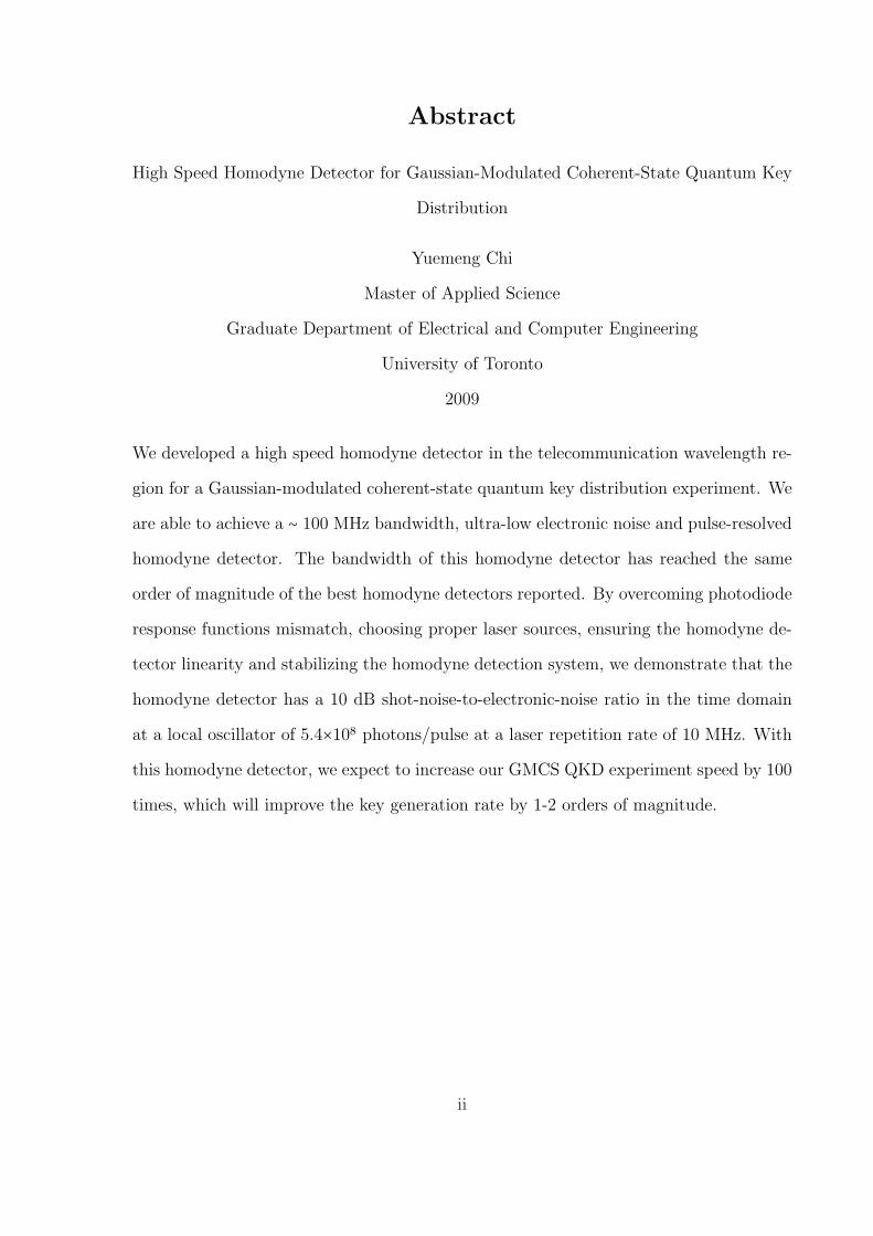
Abstract
High Speed Homodyne Detector for Gaussian-Modulated Coherent-State Quantum Key
Distribution
Yuemeng Chi
Master of Applied Science
Graduate Department of Electrical and Computer Engineering
University of Toronto
2009
We developed a high speed homodyne detector in the telecommunication wavelength re-
gion for a Gaussian-modulated coherent-state quantum key distribution experiment. We
are able to achieve a � 100 MHz bandwidth, ultra-low electronic noise and pulse-resolved
homodyne detector. The bandwidth of this homodyne detector has reached the same
order of magnitude of the best homodyne detectors reported. By overcoming photodiode
response functions mismatch, choosing proper laser sources, ensuring the homodyne de-
tector linearity and stabilizing the homodyne detection system, we demonstrate that the
homodyne detector has a 10 dB shot-noise-to-electronic-noise ratio in the time domain
at a local oscillator of 5.4�108 photons/pulse at a laser repetition rate of 10 MHz. With
this homodyne detector, we expect to increase our GMCS QKD experiment speed by 100
times, which will improve the key generation rate by 1-2 orders of magnitude.
ii

Dedication
First and foremost I owe my deepest gratitude to my supervisors, Professor Hoi-
Kwong Lo and Professor Li Qian, who have supported me thoughout my research with
their patience and knowledge. I attribute my master work to their encouragement and
effort. Without their support, this thesis would not have been completed. It is an honor
for me to work with them during my last two years’ study. One simply could not wish
for a better or friendlier supervisor.
I am also deeply appreciate the help and advice received from Doctor Bing Qi, who
essentially teaches me everything in an optical and electrical lab. I am grateful to Doctor
Bing Qi for his knowledge and many useful discussions that motivated me.
Special thanks are extended to Professor J. Stewart Aitchison, Professor Lacra Pavel,
and Professor Joyce Poon for their time, advice, and willingness to serve on the commit-
tee.
I would like to show my gratitude to Professor Alex Lvovsky at University of Calgray
for generously providing the homodyne detector electronic design and printed circuit
board layout. I also thank Professor SunHyun Youn and Nitin Jain for their kind help
in building the homodyne detector circuit and sharing a lot of construction experience.
I would also extend my thanks to Liang Tian, who has helped a lot in tuning the
homodyne detector circuit. I also would like to acknowledge Professor Namdar Saniei
and Doctor Wen Zhu for helpful discussions. It is a pleasure to thank a friendly and
cheerful group of fellow students, Viacheslav Burenkov, Wei Cui, Chi-Hang Fred Fung,
Junbo Han, Wolfram Helwig, Kenny Ho, Dongpeng Kang, Xiongfeng Ma, Jason Ng,
Wing-Chau Ng, Chris Sapiano, Peyman Sarrafi, Gigi Wong, Fei Ye, Jiawen Zhang, Lijun
Zhang, and Eric Zhu for their support and friendship. I also thank 3GMetalWorx Inc.
for providing a professional shielding metal box for the homodyne detector circuit.
Furthermore, I would like to thank Ms. Diane Silva and Ms. Linda Liu for their
efficient and professional administrative work.
iii

Finally and most importantly, this thesis would not have been possible without the
endless love and support from my family. This thesis is dedicated to my husband and
my parents.
iv

Contents
1 Introduction 1
1.1 Background . . . . . . . . . . . . . . . . . . . . . . . . . . . . . . . . . . . . . . 1
1.2 Motivation: high speed homodyne detector . . . . . . . . . . . . . . . . . . . 6
1.3 Objective . . . . . . . . . . . . . . . . . . . . . . . . . . . . . . . . . . . . . . . 7
1.4 Organization . . . . . . . . . . . . . . . . . . . . . . . . . . . . . . . . . . . . . 8
2 Review of GMCS QKD and Homodyne Detection 9
2.1 Gaussian-modulated coherent-state quantum key distribution . . . . . . . . 9
2.1.1 Protocol . . . . . . . . . . . . . . . . . . . . . . . . . . . . . . . . . . . . 9
2.1.2 State of the art . . . . . . . . . . . . . . . . . . . . . . . . . . . . . . . 12
2.2 Homodyne detection . . . . . . . . . . . . . . . . . . . . . . . . . . . . . . . . . 14
2.2.1 Introduction . . . . . . . . . . . . . . . . . . . . . . . . . . . . . . . . . 14
2.2.2 State of the art . . . . . . . . . . . . . . . . . . . . . . . . . . . . . . . 19
2.3 Summary . . . . . . . . . . . . . . . . . . . . . . . . . . . . . . . . . . . . . . . 21
3 GMCS QKD over 20 km Fiber 22
3.1 Experimental setup . . . . . . . . . . . . . . . . . . . . . . . . . . . . . . . . . 22
3.2 Secure key rate formula . . . . . . . . . . . . . . . . . . . . . . . . . . . . . . . 24
3.3 Results . . . . . . . . . . . . . . . . . . . . . . . . . . . . . . . . . . . . . . . . . 27
3.4 Discussions . . . . . . . . . . . . . . . . . . . . . . . . . . . . . . . . . . . . . . 33
3.5 Summary . . . . . . . . . . . . . . . . . . . . . . . . . . . . . . . . . . . . . . . 35
v

4 High Speed Homodyne Detector 37
4.1 Requirement of a homodyne detector in GMCS QKD . . . . . . . . . . . . . 37
4.2 High speed homodyne detector design . . . . . . . . . . . . . . . . . . . . . . 38
4.2.1 Homodyne detector optical setup in fiber . . . . . . . . . . . . . . . . 38
4.2.2 Homodyne detector electrical circuit . . . . . . . . . . . . . . . . . . . 39
4.3 Challenges . . . . . . . . . . . . . . . . . . . . . . . . . . . . . . . . . . . . . . . 40
4.3.1 Low electronic noise . . . . . . . . . . . . . . . . . . . . . . . . . . . . . 41
4.3.2 Different photodiode response functions . . . . . . . . . . . . . . . . . 42
4.3.3 Linearity . . . . . . . . . . . . . . . . . . . . . . . . . . . . . . . . . . . 45
4.3.4 Laser source . . . . . . . . . . . . . . . . . . . . . . . . . . . . . . . . . 47
4.3.5 Optical stability . . . . . . . . . . . . . . . . . . . . . . . . . . . . . . . 52
4.4 Summary . . . . . . . . . . . . . . . . . . . . . . . . . . . . . . . . . . . . . . . 54
5 Performance of the Homodyne Detector 55
5.1 Experimental plan . . . . . . . . . . . . . . . . . . . . . . . . . . . . . . . . . . 56
5.2 Measurement with CW light . . . . . . . . . . . . . . . . . . . . . . . . . . . . 56
5.2.1 Experimental setup . . . . . . . . . . . . . . . . . . . . . . . . . . . . . 57
5.2.2 Noise measurement in the time domain . . . . . . . . . . . . . . . . . 58
5.2.3 Noise measurement in the frequency domain . . . . . . . . . . . . . . 60
5.3 Measurement with pulsed light . . . . . . . . . . . . . . . . . . . . . . . . . . 62
5.3.1 Pulsed laser source . . . . . . . . . . . . . . . . . . . . . . . . . . . . . 62
5.3.2 Noise measurement in the time domain . . . . . . . . . . . . . . . . . 63
5.3.3 Noise measurement in the frequency domain . . . . . . . . . . . . . . 73
5.4 Conclusions and discussions . . . . . . . . . . . . . . . . . . . . . . . . . . . . 77
6 Conclusion and Future Work 81
6.1 Significance and contribution . . . . . . . . . . . . . . . . . . . . . . . . . . . . 81
6.2 Future work . . . . . . . . . . . . . . . . . . . . . . . . . . . . . . . . . . . . . . 83
vi

List of Tables
1.1 Secure key rate (bit) per pulse for GMCS [1], decoy state [2] and DPS
[3] protocols over 5-km telecommunication fiber. Secure key rates for de-
coy state and DPS protocols are simulation results based on experimental
conditions. . . . . . . . . . . . . . . . . . . . . . . . . . . . . . . . . . . . . . . . 5
3.1 Parameters used in the key rate simulation , from Ref. [1]. The length of
the fiber is 5 km. . . . . . . . . . . . . . . . . . . . . . . . . . . . . . . . . . . . 31
3.2 20-km GMCS QKD parameters and results (e: experimental result; c:
calculated result) . . . . . . . . . . . . . . . . . . . . . . . . . . . . . . . . . . . 33
3.3 Secure key rate in our GMCS QKD experiment and in Ref. [4] over 20-km
fiber. rep. :repetition . . . . . . . . . . . . . . . . . . . . . . . . . . . . . . . . 33
4.1 Specifications of FGA04 InGaAs photodiode (typical values). . . . . . . . . 39
4.2 Specifications of the two lasers used in photodiode linearity test . . . . . . . 49
5.1 Parameters in the key rate simulation (given in Ref. [1]). Here we assume
εA and Nleak are the same for high-speed and low-speed GMCS QKD
experiments. . . . . . . . . . . . . . . . . . . . . . . . . . . . . . . . . . . . . . . 71
6.1 HD peformance comparison between our group and Ref. [5] . . . . . . . . . 82
vii

List of Figures
1.1 One-time-pad scheme . . . . . . . . . . . . . . . . . . . . . . . . . . . . . . . . 2
1.2 Alice prepares four photons with arbitrary polarizations. Eve taps them
from the channel and uses her basis (horizontal and vertical basis) to
measure them. The polarization of those photons will collapse to Eve’s
basis. Thus, Eve cannot perfectly duplicate those states. . . . . . . . . . . . 3
2.1 GMCS QKD protocol. . . . . . . . . . . . . . . . . . . . . . . . . . . . . . . . 11
2.2 Schematic of a homodyne detection. BS: beam splitter; SIG: signal; LO:
local oscillator; PD: photodiode; φ: introducing a phase between the signal
and the LO; Black line: optical path; Blue line: electrical path; Dashed
box: homodyne detector . . . . . . . . . . . . . . . . . . . . . . . . . . . . . . 15
2.3 LO and signal states in the phasor space. . . . . . . . . . . . . . . . . . . . . 16
2.4 Scheme of a photocurrent subtraction. PD: photodiode . . . . . . . . . . . . 19
3.1 Schematic of the GMCS QKD system. L: 1550 nm CW fiber laser, PC1−5:
polarization controllers; PBS1−3: polarization beam splitters or combiners;
AM0−1: amplitude modulators; PM1−2: phase modulators; SW1−2:optical
switches; AOM+(AOM−): upshift(downshift) acousto-optic modulators;
VOA1−2: variable optical attenuators; ISO: isolator; C: fiber coupler; HOM:
homodyne detector [1, 6, 7] . . . . . . . . . . . . . . . . . . . . . . . . . . . . . 23
viii

3.2 Quadrature variances prepared by Alice, quadrature variances measured
by Bob, and equivalent input noise χ. Quadrature variance prepared by
Alice, and equivalent input noise χ are referred to the input. Noise on
Bob’s side is referred to the output. . . . . . . . . . . . . . . . . . . . . . . . 25
3.3 QKD experimental results. The equivalent input noise has been deter-
mined experimentally to be χ = 6.13[6, 7]. . . . . . . . . . . . . . . . . . . . . 28
3.4 Determine δ by using a high modulation variance VA � 40000 and a weak
LO (105 photon/pulse). The result is δ = 0.0049 . . . . . . . . . . . . . . . . 29
3.5 Noise of the balanced HD as a function of LO power. With a LO of
1.2�107 photons/pulse, the electronic noise is 6.8 dB below the shot noise
(plot with raw data obtained from [1]) . . . . . . . . . . . . . . . . . . . . . . 30
3.6 Secure key rate as a function of the electronic noise (in shot noise unit)
under the “general model”. Parameters in this simulation are in Table 3.1 . 31
3.7 The leakage from LO to signal. LO: local oscillator; SIG: signal; LE:
leakage; PBS: polarization beam splitter; LO is 5-6 orders of magnitude
higher than signal. The leakage from signal to LO is negligible. Arrowed
lines indicate the polarization of the beam . . . . . . . . . . . . . . . . . . . . 32
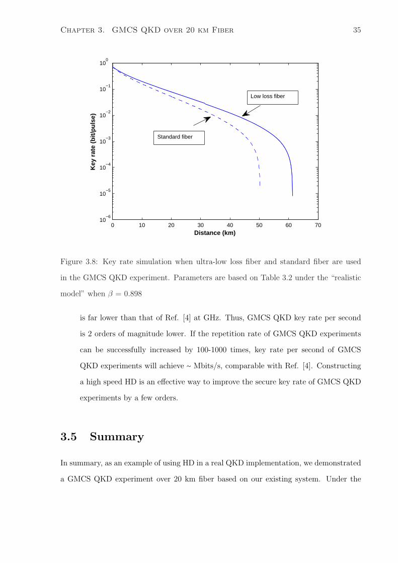
3.8 Key rate simulation when ultra-low loss fiber and standard fiber are used
in the GMCS QKD experiment. Parameters are based on Table 3.2 under
the “realistic model” when β = 0.898 . . . . . . . . . . . . . . . . . . . . . . . 35
3.9 Key rate simulation with excess noise and in the absence of excess noise.
Parameters are based on Table 3.2 under the “realistic model” when β =
0.898 . . . . . . . . . . . . . . . . . . . . . . . . . . . . . . . . . . . . . . . . . . 36
4.1 Homodyne detection setup in the telecommunication wavelength. LO:
local oscillator; OVD: optical variable delay; FC: 50:50 fiber coupler; VOA:
variable optical attenuator; PD: photodiode; AMP: electronic amplifiers. . 39
ix

4.2 A simplified homodyne detector circuit. PD: photodiode (Thorlabs,FGA04);
OPA847: operational amplifier (Texas Instrument) . . . . . . . . . . . . . . 40
4.3 Photo of the circuit board of the homodyne detector. Two FGA04 photo-
diodes are in the upper left corner. . . . . . . . . . . . . . . . . . . . . . . . . 42
4.4 Customized metal box for shielding, constructed by 3GMetalWorx Inc..
Dimensions (cm): 8.12�6.67�4.22; Thickness (cm): 0.0406 . . . . . . . . . . 43
4.5 Photodiode impulse responses test. (a)Photodiode impulse responses test
setup. Laser: Picoquant PDL 800-B, pulse width: �30-50 ps; RLoad = 50
Ohm. Laser pulses are sent to the photodiode and the output electrical
voltage V0 is measured by an oscilloscope. (b) V0 as a function of time
for ten photodiodes. We acknowledge Liang Tian’s testing work in this
experiment. . . . . . . . . . . . . . . . . . . . . . . . . . . . . . . . . . . . . . . 44
4.6 Residual signals at the output of the HD, after balancing the two signals
to the photodiodes. Laser: PriTel Mode-lock femsto-second fiber laser;
pulse width: 0.7 ps - 1.2 ps; LO power = 13.8 μ W. Horizontal scale: 20
ns/div; Vertical scale: 10 mV/div. . . . . . . . . . . . . . . . . . . . . . . . . 45
4.7 Photodiode impulse response with (a) pulse width: 0.7-1.2 ps; horizontal
scale: 2 ns/div; vertical scale: 50 mV/div (b) pulse width: 50 ns; edge
time: 15 ns; horizontal scale: 20 ns/div; vertical scale: 2 mV/div . . . . . 46
4.8 (a) Circuit linearity test circuit. It is the amplification part of the circuit
in Fig. 4.2. OPA847: electronic amplifier; (b) Circuit linearity test setup.
Electrical pulses (generated by a function generator, repetition rate: 10
MHz; pulse width: 50 ns) is sent to the circuit in (a). The output is
measured by an oscilloscope. . . . . . . . . . . . . . . . . . . . . . . . . . . . . 47
4.9 Output peak voltage as a function of the input peak voltage for both
positive and negative signals. The slope (HD electronic amplifiers voltage
gain) is 22. The straight line is the linear fit. . . . . . . . . . . . . . . . . . . 48
x
4.10 (a) Photodiode linearity test circuit. PD: photodiode; (b) Photodiode lin-
earity test setup. Laser I or II pulses are sent to one of the photodiodes.
An oscilloscope is used to measure the output peak voltage. PD: photo-
diode; Switch is connected with port 1,2 to test the photodiode linearity,
while connected with port 3 to measure the optical power. . . . . . . . . . . 50
4.11 Photodiode output peak voltage as a function of the photon number per
pulse with laser I (� 1 ps pulse width) as a source. . . . . . . . . . . . . . . . 51
4.12 Photodiode output peak voltage as a function of the photon number per
pulse for laser II (� 50 ns pulse width) as a source . . . . . . . . . . . . . . . 52
5.1 Experimental setup with CW LO (NP Photonics). CW L: 1550 nm CW
fiber laser; VOA1-2: variable optical attenuators; LO: local oscillator; FC:
50:50 fiber coupler; OVD: optical variable delay; PD: photodiodes; AMP:
HD electronic amplifiers; OSC: oscilloscope (Lecroy); RFSA: RF spectrum
analyzer (HP 8564E); Dashed line box: homodyne detector. . . . . . . . . . 57
5.2 Calibration setup to get the balanced condition. Pulsed L: 1550 nm Pri-
Tel pulsed femto second laser; VOA1-2: variable optical attenuators; LO:
local oscillator; FC: 50:50 fiber coupler; OVD: optical variable delay; PD:
photodiodes; AMP: HD electronic amplifers; OSC: oscilloscope (Lecroy);
RFSA: RF spectrum analyzer (HP 8564E); Dashed line box: homodyne
detector. . . . . . . . . . . . . . . . . . . . . . . . . . . . . . . . . . . . . . . . . 58
5.3 Oscilloscope graph for HD noise measurement at a CW LO power of 0.187
mW. Horizontal scale: 5 μs/div. Vertical scale: 2 mV/div. . . . . . . . . . . 59
5.4 Voltage variance as a function of the CW LO power in the time domain.
The red line has a slope of 1. . . . . . . . . . . . . . . . . . . . . . . . . . . . . 60
xi

5.5 RF spectrum analyzer background noise spectrum (lowest curve), HD
electronic noise spectrum (second lowest curve) and HD noise spectra at
CW LO powers of 6.4400, 4.1400, 2.5380, 1.5960, 1.0180, 0.6460, 0.4140,
0.2528,0.1592,0.1014,0.0640,0.0410 and 0.0252 mW (from the highest to
the third lowest curve). Resolution bandwidth: 1 MHz . . . . . . . . . . . . 61
5.6 Noise spectrum from DC to 10 MHz at an LO power of 0.3 mW. Resolution
bandwidth: 1 MHz . . . . . . . . . . . . . . . . . . . . . . . . . . . . . . . . . 62
5.7 HD noise power and shot noise power as a function of CW LO in the
frequency domain. The red line has a slope of 1. . . . . . . . . . . . . . . . . 63
5.8 Experimental setup of HD noise measurement in the time domain. CW
L: 1550 nm CW fiber laser; VOA1-2: variable optical attenuators; LO:
local oscillator; FC: 50:50 fiber coupler; OVD: optical variable delay; PD:
photodiodes; AMP: HD electronic amplifiers; OSC: oscilloscope (Lecroy);
Dashed line box: homodyne detector. . . . . . . . . . . . . . . . . . . . . . . . 64
5.9 HD output waveform under the balanced condition at an LO power of
0.786 mW. Horizontal scale: 50 ns/div. Vertical scale: 50 mV/div. The
square box on this graph indicates one cycle. . . . . . . . . . . . . . . . . . . 64
5.10 One measurement frame at an LO power of 0.4 mW. Horizontal scale: 10
mV/div, Vertical scale: 5 μs/div. . . . . . . . . . . . . . . . . . . . . . . . . . 66
5.11 Data processing procedure (LO = 0.77 mW). (a) 500 original curves (one
frame) S; (b) Background curve (i.e., the average curve) of S; (c) 500
processed curves (one frame) T . . . . . . . . . . . . . . . . . . . . . . . . . . . 67
5.12 HD noise variance and shot noise variance as a function of the pulsed LO
power in the time domain. The red line has a slope of 1. . . . . . . . . . . . 69
5.13 Correlation coefficient between nth (X) and n +mth (Y) pulses at an LO
power of 0.77 mW . . . . . . . . . . . . . . . . . . . . . . . . . . . . . . . . . . 70
xii

5.14 Quadrature value of nth pulse X�n� and that of n+1 pulse Y �n� =X�n+1�at an LO power of 0.77 mW . . . . . . . . . . . . . . . . . . . . . . . . . . . . 71
5.15 Key rate simulation as a function of the transmission distance with a
high-speed HD (running at 10 MHz repetition rate) and a low-speed HD
(running at 100 kHz repetition rate) . . . . . . . . . . . . . . . . . . . . . . . 72
5.16 Experimental setup in the frequency domain. CW L: 1550 nm CW fiber
laser; VOA1-2: variable optical attenuators; AM: amplitude modulator;
PC: polarization controller; LO: local oscillator; FC: 50:50 fiber coupler;
OVD: optical variable delay; PD: photodiode; AMP: HD electronic am-
plifers; RFSA: RF spectrum analyzer (HP 8564E); Dashed line box: ho-
modyne detector. . . . . . . . . . . . . . . . . . . . . . . . . . . . . . . . . . . . 73
5.17 Noise spectrum at an LO power of 0.786 mW. Frequency range: DC to
100 MHz. Resolution bandwidth: 100 kHz. . . . . . . . . . . . . . . . . . . . 74
5.18 Noise spectrum at an LO power of 24.56 μW when (a)two photodiodes are
illuminated; (b)one photodiode is blocked. Resolution bandwidth: 100 kHz 75
5.19 Noise spectra at different LO powers. Frequency span: 5 to 6 MHz. Reso-
lution bandwidth: 10 kHz. LO powers are 0.0029, 0.0072, 0.0142, 0.0292,
0.0458, 0.0721, 0.1136, 0.1784, 0.2920, 0.4580, 0.7180, 1.1340, 1.7760,
2.9200 mW from the lowest curve to the highest curve, respectively. . . . . 76
5.20 Noise power as a function of the LO power in the frequency domain. The
red line has a slope of 1. . . . . . . . . . . . . . . . . . . . . . . . . . . . . . . 77
6.1 A self-differencing scheme in homodyne detection. Red pulses are optical
pulses and blue pulses are electrical pulses. . . . . . . . . . . . . . . . . . . . 84
xiii

Chapter 1
Introduction
In the information era, cryptography has become extremely important for governments,
the military, businesses and the public. It allows people to achieve secure communications
between different places without worries of information leakage. Quantum cryptography
(quantum key distribution) has been proved to be unconditionally secure and has been
studied widely in the past decade[8, 9]. To improve the quantum information trans-
mission speed, the construction of a high speed homodyne detector (HD) for Gaussian-
modulated coherent-state (GMCS) quantum key distribution (QKD) experiments will be
investigated in this thesis. In this chapter, background knowledge on GMCS QKD and
homodyne detection will be presented.
1.1 Background
How to achieve a secure communication has been an important question for thousands of
years. In a secure communication, Alice and Bob would like to communicate in a secure
manner in the presence of an eavesdropper, traditionally called Eve. Many encryption
techniques have been invented, however, their securities are not completely guaranteed.
For example, one famous encryption scheme called RSA, invented by Rivest, Shamir and
Adleman in 1978 [10], is widely used in payment card chip technology. The RSA idea
1

Chapter 1. Introduction 2
Figure 1.1: One-time-pad scheme
employs that for certain functions f�x�, it is easy to compute f�x� given x, but difficult
to recover x given the value of f�x�. For instance, one can easily compute 97 �83 =
8051, while it requires a lot of effort to find out the prime factors of 8051. Security
of RSA is based on the computational complexity assumption of factorization of large
integers. However, this assumption can be violated by fast factoring using a quantum
computer[11], hence the security is threatened.
As a significant development to realize secure communication, the one-time-pad scheme
was first proposed by G. Vernam in 1917 [12] and has since been proved secure by C.
Shannon [13]. In this scheme, shown in Fig. 1.1, Alice and Bob share a binary key
string (pad) with a length equal to the original message. Alice first performs an XOR
operation (i.e. addition modulo two) between every bit of the original message and every
corresponding bit of the key to generate an encrypted message. She then transmits this
encrypted message to Bob. Bob decodes the original message by performing an XOR
operation between the encrypted message and the same key as Alice used to encrypt the
message. The key has to be as long as the message, and cannot be reused. Whenever
Alice wants to send a new message, she needs to find a way to distribute the key to Bob
without leaking any information about the key to Eve. This is called the key distribu-

Chapter 1. Introduction 3
Figure 1.2: Alice prepares four photons with arbitrary polarizations. Eve taps them
from the channel and uses her basis (horizontal and vertical basis) to measure them. The
polarization of those photons will collapse to Eve’s basis. Thus, Eve cannot perfectly
duplicate those states.
tion problem. Therefore, the problem of secure communication with the one-time-pad
encryption becomes the problem of key distribution. Solving the key distribution prob-
lem is challenging because classical key information (i.e. the key string is represented
by classical bits) can be tapped and duplicated during transmission through a classical
communication channel (e.g. a fiber-optic link) without being detected by Alice and Bob.
The key distribution problem is solved by the proposal of quantum key distribution
(QKD)[8, 9, 14, 15]. The security of QKD is based on fundamental quantum mechanical
principles, such as the quantum no-cloning theorem [16, 17, 18] , which states that an
arbitrary quantum state cannot be perfectly duplicated, and the Heisenberg uncertainty
principle which states that two non-commuting observables cannot be precisely known
together. For example, if Alice uses the polarization of a single photon to encode key
information and sends it to Bob, Eve may intercept this single photon from the channel
and measure the polarization of the single photon in an orthogonal basis. However, the
polarization of the single photon will collapse to one of the basis states chosen by Eve
and will not be able to be perfectly duplicated (shown in Fig. 1.2). Another example
is the Heisenberg uncertainty principle ΔxΔp � h4π , stating that the position (x) and

Chapter 1. Introduction 4
momentum (p) of a particle (or wave) cannot be precisely known at the same time. If
Eve is trying to measure the position, she will inevitably introduce more uncertainty to
the momentum. If Alice and Bob monitor the uncertainty of both x and p, they will be
able to detect Eve if the added noise on x or p is above a threshold. Due to the difficulty
of encoding information in the position and momentum of a particle (or wave), a scheme
of encoding information in the amplitude and phase quadrature of the electric field is
developed [19].
QKD has been studied intensively for more than one decade [8, 9, 14, 15, 20, 21, 22].
There are many impressive progresses in both theory and experiment [14, 19, 23, 24,
25, 26]. QKD systems have been implemented with single photon source [14, 15, 27],
in which properties of single photons (polarization, phase, etc) are used to encode key
information, and coherent states source [19, 28], in which information is encoded in the
measurable quantities of a coherent state, such as the amplitude and phase quadratures
of a faint laser pulse (weak coherent state).
In the best-known BB84 QKD protocol [14], a perfect single photon source is used
to guarantee the security. Unfortunately, a single photon state is difficult to generate in
practice, despite tremendous efforts [29, 30, 31]. In practical systems, highly attenuated
coherent laser sources that have a non-negligible chance to emit single-photon pulses are
used. However, with such highly attenuated laser sources, unconditional security cannot
be directly applied because of their finite probability of emitting multi-photon pulses.
To solve this problem, special techniques based on currently available highly attenuated
coherent laser sources, such as decoy state protocol, have been implemented to improve
the key rate [23, 32, 33, 34, 35, 36, 37, 38].
To avoid the requirement for a true single-photon source, coherent states QKD has
been proposed in the past few years as a promising alternative to the commonly utilized
single photon QKD. QKD based on Gaussian-modulated coherent-state (GMCS) protocol
has recently attracted increasing interests [19, 39, 40, 41, 42]. This protocol will be

Chapter 1. Introduction 5
discussed in detail in Section 2.1.1. There are several advantages of this protocol over
single photon QKD. [43, 44].
1. The coherent state can be produced easily by a practical laser source, while the
perfect single photon source is still unavailable.
2. The homodyne detector in the GMCS QKD can be constructed using high efficient
PIN photodiodes [39], while the efficiency of the single photon detector in the
telecommunication wavelength region is low.
3. More than one bit of information could be transmitted by sending one coherent
state and hence GMCS protocol could achieve a high key rate.
GMCS QKD has a distinct advantage in its potential application in achieving a higher
key rate over a short distance [19]. A comparison of the key rate per pulse for GMCS,
decoy state and differential phase shift (DPS, another example of single photon QKD)
QKD is shown in Table 1.1. More detailed comparison between GMCS QKD and single
photon QKD can be found in Ref. [45].
As shown in Table 1.1, the secure key rate per pulse over a short distance in the
GMCS QKD experiment is two orders of magnitude higher than those in single photon
QKD experiments (decoy state and DPS QKD). However, the current experimental im-
plementation of GMCS QKD is below 1 MHz repetition rate [1, 43], much lower than
Table 1.1: Secure key rate (bit) per pulse for GMCS [1], decoy state [2] and DPS [3]
protocols over 5-km telecommunication fiber. Secure key rates for decoy state and DPS
protocols are simulation results based on experimental conditions.
Secure key rate per pulse
GMCS [1] 0.3
Decoy state [2] �0.002
DPS [3] �0.001

Chapter 1. Introduction 6
single photon QKD at a few GHz repetition rate [4, 46], thus the secure key rate per
second in a GMCS QKD experiment is still lower than that of a high speed single photon
QKD experiment. Development of a high speed GMCS QKD system will be an interest-
ing research direction in future experimental QKD implementation. Since the repetition
rate of GMCS QKD experiments is fundamentally limited by the speed of the homodyne
detector (HD, to be shown in Sections 1.2 and 2.1.2), a high speed HD that meets the
requirements of GMCS QKD experiments should be developed as the first step to achieve
this long term goal.
1.2 Motivation: high speed homodyne detector
In GMCS QKD experiments, key information is encoded in electric field quadratures of
weak coherent states by Alice. On Bob’s side, he will measure the quadrature values using
a homodyne detection technique. Homodyne detection is extremely useful since it can
be used to characterize the electric field of an optical signal, even if it is a non-classical
signal, such as squeezed state. This unique characteristic makes homodyne detection a
popular implementation in quantum applications [47, 48, 49].
Homodyne detection has been used for many years in optical communication [49, 50].
There are also commercialized fast (up to 40 GHz) balanced receivers that can be used
in homodyne detection [51, 52]. Unfortunately, they are not suitable for GMCS QKD
experiments. In classical optical communications, usually strong light is sent to the
signal port. For example, -20 dBm signal is used in Ref. [53] and 0 dBm signal is used
in Ref. [54]. However, in GMCS QKD experiments, the signal pulse is very weak, less
than -95 dBm in Ref. [1] and -90 dBm in Ref. [43] . Therefore, the homodyne detector
(HD) used in GMCS QKD experiments should be very sensitive, which requires ultra-
low electronic noise of the HD. In addition to the low noise requirement, in GMCS QKD
experiments, HDs need to be able to measure the individual pulse in the time domain

Chapter 1. Introduction 7
since key bits are encoded in every signal pulse. Owing to these requirements, most
research groups have to develop their own HDs for quantum information and quantum
optics implementations [40, 43, 47, 48, 55]. To date, only a few groups have been able to
construct broad bandwidth HDs (� 100−250 MHz) for quantum measurements [5, 47, 56,
57], however, none is demonstrated at 1550 nm wavelength. High-speed HDs operating
in the telecommunication wavelength region that can be used in quantum optics and
quantum information are still lacking. In this thesis, my goal is to develop a high speed
HD in the telecommunication wavelength that will be suitable for high speed GMCS
QKD experiments.
1.3 Objective
The long term objective is to experimentally develop a high speed QKD system based on
GMCS protocol. This will be achieved by developing high speed modulations, detections,
data acquisitions, classical data processing algorithms, etc (to be discussed in Section
2.1.2). As the first stage to achieve this objective, the goal of my thesis is to enable a
fully-fiber based high speed GMCS QKD system by constructing a fast detection system:
homodyne detector (HD) in the telecommunication wavelength region.
My research is carried out with the following objectives.
• Establish the requirements and challenges of an HD for a high-speed GMCS QKD
system.
• Provide both electrical and optical designs of a high speed HD to meet those re-
quirements.
• Construct and test the HD, and outperform the previous demonstrations reported
in the literature.

Chapter 1. Introduction 8
• Evaluate HD performance in real QKD and suggest directions for future high speed
GMCS QKD experimental implementation.
1.4 Organization
The thesis is organized as follows: I briefly review the development of GMCS QKD and
homodyne detection in Chapter 2, from principle to the state of the art. In Chapter 3,
I will discuss an example of using a custom-designed low speed HD in a 20-km GMCS
QKD implementation over an existing system. The main work of this thesis is discussed
in Chapter 4 and Chapter 5. In Chapter 4, requirements of a high speed HD that can
be used in high speed GMCS QKD experiments are presented. Challenges and solutions
of constructing a high speed HD are also discussed in this chapter. In Chapter 5, I will
present the testing results of our constructed HD in both time and frequency domains,
with CW and pulsed light, respectively. Our results show that this HD has a bandwidth
of � 100 MHz, which will enable GMCS QKD experiments at a repetition rate of 10
MHz. The expected key rate of GMCS QKD experiments with this HD will be increased
by 1-2 orders of magnitude, which is comparable to the high speed QKD based on single
photon protocols. In Chapter 6, I will summarize the thesis, discuss the significance of
the work and suggest future work for developing a high speed GMCS QKD system.

Chapter 2
Review of GMCS QKD and
Homodyne Detection
2.1 Gaussian-modulated coherent-state quantum key
distribution
Over the past few years, quantum key distribution (QKD) using Gaussian-modulated
coherent-state (GMCS) protocol has drawn a lot of attention [19, 39, 40, 41, 42]. The
uncertainty principe, which states that the amplitude quadrature (x) and the phase
quadrature (p) of a coherent state cannot be precisely known simultaneously, is the foun-
dation of GMCS QKD. Any eavesdropping of one quadrature will introduce additional
noise to the other quadrature. Alice and Bob are able to detect Eve if they monitor the
variances of x and p together. In this section, I will give an overview of the GMCS QKD
protocol and the state of the art of this topic.
2.1.1 Protocol
In the classical electromagnetism, a light field can be characterized by x cosωt + p sinωt,
where ω is the angular frequency, and x and p are amplitude and phase quadratures.
9

Chapter 2. Review of GMCS QKD and Homodyne Detection 10
When the light intensity is very weak and the quantum effect is considered, the measure-
ment of one quadrature will introduce more uncertainty to the other quadrature. In the
GMCS QKD, Alice encodes x and p on each bit and Bob randomly chooses x or p to
decode information. Eve does not know which basis Bob will select to perform measure-
ment. If Eve eavesdrops in a random basis, according to the uncertainty principle, her
measurement of x (p) will disturb the variable p (x), i.e. Eve cannot simultaneously re-
duce measurement error on both quadratures. Therefore, the presence of Eve inevitably
introduces additional noise in Bob’s measurements, which we call excess noise. After the
key transmission, by comparing some of Bob’s measurement results with the x, p values
prepared by Alice, Bob can estimate the excess noise, which is attributed to Eve. Hence,
Bob can estimate the amount of information leaked to Eve. Alice and Bob then distill
the secure information by a classical data processing. Note that, the difference between
GMCS QKD and classical optical communication is that weak (quantum) signal is used
in GMCS QKD. If the excess noise in GMCS QKD is above a threshold, no secure key
can be transmitted. An example of using a strong signal in GMCS QKD will be shown
in Fig. 3.4 of Section 3.3, in which no positive secure key is generated.
The protocol of the GMCS QKD is described as follows (shown in Fig. 2.1) [19, 43,
39, 45, 58].
1. Alice generates two random sets of continuous variables x and p with a Gaussian
distribution that has a zero average (variance = VAN0, N0 is the shot noise unit).
For a continuous Gaussian noise channel, a Gaussian distribution of the input will
yield an optimal channel capacity [59]. In the GMCS QKD, Alice encodes random
bits (key information) by modulating the amplitude quadrature (x) and the phase
quadrature (p) of weak coherent states �x + ip� (typically less than 100 photons
in each pulse) with her Gaussian distributed sets x, p. Experimentally this is
realized by modulating the intensity and the phase of each pulse. On the receiver’s
side, Bob measures either x or p quadrature of the weak coherent states randomly

Chapter 2. Review of GMCS QKD and Homodyne Detection 11
Figure 2.1: GMCS QKD protocol.
by using a homodyne detection. Note that, the signal cannot be amplified before
being detected, since quantum coherent states cannot be perfectly cloned without
paying penalty (adding excess noise).
2. Through an authenticated public channel (Eve can listen to the information but
cannot modify), Bob informs Alice about the quadratures he picked. Alice then
discards the quadratures that were not measured by Bob. At this stage, Alice
shares a set of correlated Gaussian variables (called the ”raw key”) with Bob.
3. Alice and Bob then publicly compare a random sample of their raw key to evaluate
the transmission efficiency of the quantum channel ηG (including channel efficiency
G and Bob’s system efficiency η), and the excess noise ε of the QKD system. Excess
noise is the noise above the vacuum noise level associated with channel losses [39].
It reflects possible leakage information to Eve. Based on the parameters, Alice and
Bob can evaluate their mutual information IAB and the information obtained by
Eve IBE1[19, 60]. This stage is a classical data processing process and can be
1Here, we assume the secure key is made of Bob’s data. Bob will publish some of his measurements

Chapter 2. Review of GMCS QKD and Homodyne Detection 12
divided into reconciliation (correcting the errors while minimizing the information
revealed to Eve. In this thesis, we only consider reverse reconciliation) and privacy
amplification (making the key secret). If the reconciliation is perfect, a secure key
of length IAB − IBE will be distilled after the classical data processing.
2.1.2 State of the art
The GMCS QKD protocol was developed in 2002 [28]. The security of the GMCS QKD
was first proven against individual attacks with direct [28] or reverse [19, 60] reconciliation
schemes. Security proofs were then given against general individual attacks [60] and
general collective attacks [43, 61, 62]. Until recently, three groups have independently
claimed they proved the unconditional security [63, 64, 65].
The first GMCS QKD experiment based on homodyne detection was demonstrated
in free space [19]. This experiment was carried out with 780 nm optical light. Hence
it did not establish the feasibility of implementation in fiber communication networks,
which are widely used for long-distance communication.
Fiber-based GMCS QKD systems over a practical distance remain challenging. So
far only two groups have implementations of the GMCS QKD over a practical distance
operated fully on fiber-based components [1, 43, 66]. To reduce excess noise arising from
the leakage from the local oscillator (LO), in Ref. [43], Mach-Zehnder interferometers
(MZIs) with largely imbalanced path lengths (80 m) were employed to separate the signal
and the leakage in the time domain (time-multiplexing scheme). However, in practice it
is quite challenging to stabilize a MZI with a large length imbalance.
One recent paper [66] by the same group reported a field test of a GMCS QKD
prototype integrated into a preinstalled quantum cryptography telecommunication net-
work. In that paper, a polarization-time multiplexing scheme is employed. The system
and Alice will modify her data according to Bob’s results. This process is called reverse reconciliationsince this flow has a reverse direction from the key transmitting flow.
Chapter 2. Review of GMCS QKD and Homodyne Detection 13
is running at 500 kHz laser repetition rate.
In contrast, our group (Experimentalists: Dr. Bing Qi and Lei-Lei Huang, under the
supervision of Profs Li Qian and Hoi-Kwong Lo) has developed a polarization-frequency-
multiplexing scheme to effectively suppress the leakage of the LO with balanced MZIs.
[1]. The system design will be described in Section 3.1. In this experiment, the laser
repetition rate is 100 kHz.
In parallel with GMCS QKD based on homodyne detection, a heterodyne detection
scheme, in which Bob measures both x and p quadratures simultaneously, was proposed
[67] (Note that, local oscillator and signal are at the same frequency. The heterodyne
detection used here is different from that defined in classical communication in which
local oscillator and signal are at different frequencies). The security proof of the GMCS
QKD based on heterodyne detection is given in Refs. [63, 68]. With this scheme, there is
no need to choose a random quadrature on Bob’s side. The experimental implementation
of GMCS QKD based on heterodyne detection has been realized in 2005 [69].
Although the GMCS QKD has a potential application in transmitting at high key
rates, so far all reported experimental systems are running below 1 MHz. There are
several limitations for a practical GMCS QKD system in achieving high speeds.
• The repetition rate of a GMCS QKD system is essentially limited by the homodyne
detector (HD) bandwidth. In QKD, each pulse quadrature encoded with Gaussian
random numbers has to be measured individually in the time domain. This will
require the response time for HD to be shorter than the inverse of the laser repeti-
tion rate. In other words, the bandwidth of the HD in the frequency domain should
be greater than the repetition rate. Intuitively, one should increase the bandwidth
of the HD to obtain a high repetition rate. However, the electronic noise is pro-
portional to the HD bandwidth [1, 40]. A wider bandwidth will result in greater
electronic noise and lead to a lower secure key rate [1].

Chapter 2. Review of GMCS QKD and Homodyne Detection 14
• The repetition rate is also limited by the speeds of computer-driven data acquisition
systems, which are typically lower than a few MHz. In Ref. [1] , a data acquisition
card (NI, PCI-6115) with a sampling rate of 10 M samples/s is employed to acquire
data. If one wants to get sufficient data points for each pulse (like 20), the maximum
repetition rate can only be a few hundreds of kHz.
• Speed of the classical reconciliation data processing will limit the GMCS QKD
speed.
Owing to the above limitations, there is no reported GMCS QKD experiment above
1 MHz repetition rate. For a GMCS QKD key transmission demonstration, if data
processing is not performed in the real time, a fast oscilloscope (40 G Samples/s) can be
used to acquire and store raw data. Considering that the HD bandwidth is a fundamental
limitation, we will develop a fast HD that can enable a high speed GMCS QKD system
in this thesis.
2.2 Homodyne detection
2.2.1 Introduction
Homodyne detection is a well-established technique for measuring the amplitude and
phase quadrature of a weak optical signal [49, 70]. Fig. 2.2 shows a schematic of homo-
dyne detection. The signal is mixed at a beam splitter (with a 50/50 splitting ratio) with
a strong local oscillator (LO)[49, 71, 72] with a defined optical phase (φ in Fig. 2.2).
This phase is introduced by a phase modulator at the LO beam in Fig. 2.2. The output
ports of the beam splitter are attached to two photodiodes. The photocurrent difference
(after the subtraction shown in Fig. 2.2) is finally amplified by an electronic amplifier.
I follow Ref. [72] to derive the output of a homodyne detection. The electric fields of
the signal ES�t� and the LO EL�t� are

Chapter 2. Review of GMCS QKD and Homodyne Detection 15
Figure 2.2: Schematic of a homodyne detection. BS: beam splitter; SIG: signal; LO:
local oscillator; PD: photodiode; φ: introducing a phase between the signal and the LO;
Black line: optical path; Blue line: electrical path; Dashed box: homodyne detector
ES�t� = ES + δXS�t� + iδPS�t�, (2.1)
and
EL�t� = EL + δXL�t� + iδPL�t��eiφ. (2.2)
where ES and EL are real time-independent terms, δXS�t� and δPS�t� (δXL�t� and
δPL�t� ) 2 are real and describe changes of amplitude and phase quadratures of the
signal (LO) field. Re ES�t�� = ES + δXS�t� is the amplitude quadrature of the signal,
while Im ES�t�� = δPS�t� is the phase quadrature of the signal. Here the spatial mode
distribution and the fast oscillating term eiωt are neglected. Fig. 2.3 shows signal and
LO states in the phasor space.φ in Fig. 2.3(same as φ in Fig. 2.2) is the relative phase
difference between the signal and the LO. For the case where the LO beam is far more
intense than the signal beam EL � ES [71, 72], the electric fields after the beam splitter
2Here, I use upper cases X and P to represent electric field quadratures, in order to distinguish withthe Gaussian distributed quadratures �x, p� used in QKD.

Chapter 2. Review of GMCS QKD and Homodyne Detection 16
Figure 2.3: LO and signal states in the phasor space.
E1�t� and E2�t� are,
E1 = 1�2�EL +ES�, (2.3)
and
E2 = 1�2�EL −ES�. (2.4)
The photocurrents from the two photodiodes are proportional to �E1�2 and �E2�2 re-
spectively,
�E1�2 = 1
2 �EL�t��2 +EL�t�E�S�t� +ES�t�E�L�t� + �ES�t��2� (2.5)
�E2�2 = 1
2 �EL�t��2 −EL�t�E�S�t� −ES�t�E�L�t� + �ES�t��2� (2.6)
The first term in Eq. (2.5) can be written as
I1 = 1
2�EL�t��2 = 1
2 EL + δXL�t� + iδPL�t�� EL + δXL�t� − iδPL�t��
� 1
2 �EL�2 + 2ELδXL�t��, (2.7)
where the small terms δX2L�t� and δP 2
L�t� are neglected.

Chapter 2. Review of GMCS QKD and Homodyne Detection 17
The second and third terms I2 and I3 are
I2 = 1
2EL�t�E�S�t� = 1
2 EL + δXL�t� + iδPL�t��eiφ ES + δXS�t� − iδPS�t��
� 1
2 ELESeiφ +ELeiφδXS�t� +ELeiφ�−iδPS�t���, (2.8)
and
I3 = 1
2ES�t�E�L�t� = 1
2 ES + δXS�t� + iδPS�t��e−iφ EL + δXL�t� − iδPL�t��
� 1
2 ESELe−iφ +ELe−iφδXS�t� +ELe−iφ�iδPS�t���, (2.9)
Here, ESδX�ESδP � is neglected compared to ELδX�ELδP �. All higher order terms in
δX�δP � are neglected.
Their sum will be
I2 + I3 = 1
2 2ELδXS�t� cosφ + 2ELδPS�t� sinφ + 2ELES cosφ�. (2.10)
Because EL � ES, I4 = 12 �ES�t��2 is neglected compared to I1.
Combining all the terms from I1 to I4, we have,
�E1�t��2 � 1
2�EL�2 + 2ELδXL�t� + 2EL �ES + δXS�t�� cosφ + δPS�t� sinφ�. (2.11)
Similarly, the results for the other photodiode can be found. We can also get the differ-
ential current i−�t� from the two photodiodes.
i−�t� = �E1�2 − �E2�2 = 2EL �ES + δXS�t�� cosφ + δPS�t� sinφ� (2.12)
The variance of this current, < i2−�t� �, is obtained by
< i2−�t� �� 4E2
L�δX2S cos2 φ + δP 2
S sin2 φ�. (2.13)
Here, since δX and δP are independent electric field fluctuations, the variance of cross
terms, such as < δXδP �, cancels out in the averaging process.
In particular, if the phase difference φ is 0 or π�2, we will obtain

Chapter 2. Review of GMCS QKD and Homodyne Detection 18
i−�t� � 2EL �ES + δXS�t�� cosφ + δPS�t� sinφ� =�����������
2ELδXS�t�, φ = 0;
2ELδPS�t�, φ = π�2.(2.14)
As a result, the current difference i−�t� will be proportional to either the X or the P
quadrature of the signal field depending on the phase difference between the signal and
the LO (0 or π�2). Because i−�t� is also proportional to the LO field, the LO should
be much stronger (typically 6 orders of magnitude stronger) than the signal to facilitate
detection of a weak signal. In GMCS QKD, Bob uses homodyne detection and measures
either X or P quadrature of the signal field by randomly introducing a phase difference
of 0 or π�2.
The variance of the current will be
< i2−�t� ��
�����������
4E2LδX2
S, φ = 0;
4E2LδP 2
S , φ = π�2.(2.15)
< i2−�t� � is proportional to the variance of the amplitude quadrature (when φ = 0) or
the phase quadrature (when φ = π�2). The variance of the electric field fluctuation is
called shot noise [71].
In a practical HD, two reverse-biased PIN-photodiodes (shown in Fig. 2.4) are em-
ployed to produce photocurrents from the optical signals, followed by a subtraction oper-
ation [48]. If pulsed light hits the two photodiodes, a positive pulse will be generated by
PD1 and a negative pulse will be generated by PD2. The intensity difference are obtained
after subtraction as shown in Fig. 2.4. Following this structure, electronic amplifiers (not
shown) are used to amplify this differential signal.
In a homodyne detection system, in addition to the shot noise due to electric field
fluctuation, electronic amplifier noise, which is affected by the gain and bandwidth, also
contributes to HD noise. Electronic noise is assumed to be independent of the intensity
of the LO if the HD circuit is operating in its linear region [73]. Shot noise and electronic

Chapter 2. Review of GMCS QKD and Homodyne Detection 19
Figure 2.4: Scheme of a photocurrent subtraction. PD: photodiode
noise are independent of each other. Thus their variances can be added, and will be
called the total noise of HD or HD noise in this thesis.
A simple experiment to measure the shot noise is to send vacuum to the signal port
of a beam splitter, measure the total noise of HD and subtract electronic noise from the
total noise of HD. Shot noise can only be detected when it exceeds HD electronic noise,
which requires a strong LO field. In most homodyne detection demonstrations with a
pulsed LO, the photon number in each pulse is typically 107-108 [1, 43, 39, 40, 48]. To
verify an HD to be shot-noise limited, we should have (1) the shot noise exceeds the
electronic noise; (2) the total noise of HD, y, is related to the LO power by an equation
of the form, y = ax+ b, where a, b are constants. The shot noise (the total noise - the HD
electronic noise) is linearly dependent on the LO power.
2.2.2 State of the art
Homodyne detection plays an important role in quantum optics [73] and quantum infor-
mation [19]. HD was originally designed for measurement in the frequency domain to

Chapter 2. Review of GMCS QKD and Homodyne Detection 20
evaluate field quadrature noise [57]. Such measurements are performed in the frequency
domain by observing a certain spectral component of the photocurrent difference signal
using an electronic spectrum analyzer. Frequency domain measurements do not give the
electric field quadrature values in the time domain. With the development of quantum
information, time domain homodyne detection has become increasingly important. How-
ever, constructing an HD for use in the time domain (the signal and the LO are both
pulsed light) is technically challenging, because
• The electronics must be fast enough to ensure temporal separation of responses to
individual laser pulses to avoid an overlap between consecutive pulses.
• Precise subtraction of the two photocurrents in the absence of the signal is necessary
in the time domain. A residual signal (incomplete subtraction of positive and
negative signals) makes our measurement difficult and may also saturate the HD
amplifiers (to be discussed in Section 4.3.2).
• The HD should provide a flat amplification profile in the frequency domain to
ensure a broad bandwidth. This frequency span should be at least from DC to the
repetition rate.
Quantum tomography experiments are one of the most important applications of time-
domain homodyne detection [5, 74]. In quantum tomography measurements, differential
photocurrent is observed in the real time and integrated over the desired temporal mode
to obtain a single value of a field quadrature. Homodyne detection is also actively used
in quantum information experiments. In GMCS QKD experiment, homodyne detection
is used by the receiver (Bob) to measure the field quadrature encoded with Gaussian
random numbers [19, 43]. In QKD based on the BB84 protocol, homodyne detection
may also be used to recover the phase information encoded on each pulse [75].
The first time domain HD were performed below 1 kHz and achieved a shot-noise-
to-electronic-noise ratio of 9 dB [76]. Hansen et al. [48] built an HD working at a
Chapter 2. Review of GMCS QKD and Homodyne Detection 21
repetition rate of 204 kHz and yielded a 14 dB shot-noise-to-electronic-noise ratio. So
far only four other groups in the world have been able to achieve a bandwidth of 100-250
MHz, which allows for tens of MHz repetition rate. Zavatta et al. [47] developed an
HD working at a repetition rate of 82 MHz with a shot-noise-to-electronic-noise ratio of
7 dB at 786 nm wavelength. During the course of my M. A. Sc. study, other groups
are also developing high speed HDs. Jain et al. [77] have demonstrated HD working at
76 MHz laser repetition rate at 800 nm wavelength. Okubo et al. [5] have developed
pulse-resolved HD at a laser repetition rate of 76 MHz with a bandwidth of more than
250 MHz at 1064 nm wavelength. Haderka et al. [57] have reported HD at a repetition
rate of 53.8 MHz at 800 nm wavelength. High speed HD with such a broad bandwidth
and a high repetition rate in the telecom wavelength region is lacking [39, 40, 55, 78]. We
will target on constructing a high speed and pulse-resolved HD in the telecommunication
wavelength region.
2.3 Summary
In this chapter, the GMCS QKD protocol and the homodyne detection principle have
been introduced. I also provided an overview of the state of the art of GMCS QKD and
homodyne detection implementations. QKD based on GMCS protocol opens a door to
very high secret key generation rates [79]. However, its current speed is fundamentally
limited by the bandwidth of the homodyne detector. To achieve a long term objective of
developing a high speed fiber-based GMCS QKD, my master thesis goal is to construct
a high speed HD at 1550 nm wavelength.

Chapter 3
GMCS QKD over 20 km Fiber
In this chapter, a 20-km fiber based GMCS QKD experiment using an existing system will
be presented as a real example of implementing HD in QKD. Comparing this result with
QKD experiments based on single photon protocols, GMCS QKD has a great advantage
in generating high key rate over a short distance. Due to the limitation of homodyne
detector bandwidth, the repetition rate of GMCS QKD is still low. To develop a high
speed GMCS QKD system, building a high speed HD is in demand.
The 20-km QKD experimental results have been published on Lasers and Electro-
optics (CLEO/QELS 2008)[6] and SPIE Optics + Photonics 2008[7], which I am a co-
author. This chapter is mainly based on the two conference papers. This work follows
a 5-km GMCS QKD experiment that has been published on Phys. Rev. A, 76, 052323
(2007). The system is developed by Dr. Bing Qi and Lei-Lei Huang, under the supervision
of Profs. Li Qian and Hoi-Kwong Lo.
3.1 Experimental setup
The schematic is shown in Fig. 3.1. In this setup, a 1550 nm continuous-wave (CW) fiber
laser (NP Photonics) is employed as the source. Alice uses an amplitude modulator (AM0
in Fig. 3.1) to generate 200-ns laser pulses at a repetition rate of 100 kHz. A polarization
22

Chapter 3. GMCS QKD over 20 km Fiber 23
beam splitter (PBS1) is used to split the pulses into a weak signal and a strong local
oscillator (LO). The splitting ratio can be controlled by a polarization controller (PC1).
In the signal arm (upper arm) of Alice’s setup in Fig. 3.1, coherent state �xA + ipA� is
modulated by the second amplitude modulator (AM1) and a phase modulator (PM1).
AM1 and PM1 are driven by Arbitrary Waveform Generators (AWG) which contain
random amplitude and phase data produced from xA, pA (Gaussian distributed with
average zero, variance = VAN0, N0 is the shot noise unit). The frequency of the LO will
be upshifted by 55 MHz by an acoustic-optic modulator (AOM+). Signal and LO will
be combined by a second polarization beam splitter (PBS2) and transmitted through a
20-km telecommunication fiber.
Figure 3.1: Schematic of the GMCS QKD system. L: 1550 nm CW fiber laser, PC1−5:
polarization controllers; PBS1−3: polarization beam splitters or combiners; AM0−1: am-
plitude modulators; PM1−2: phase modulators; SW1−2:optical switches; AOM+(AOM−):
upshift(downshift) acousto-optic modulators; VOA1−2: variable optical attenuators; ISO:
isolator; C: fiber coupler; HOM: homodyne detector [1, 6, 7]
On Bob’s side, PBS3 is used to separate signal (lower arm) and LO (upper arm). The
frequency of the LO will be downshifted by 55 MHz by a second acoustic-optic modulator
(AOM−). Bob randomly chooses either x or p with his phase modulator (PM2) driven
by a third AWG which contains a binary random file for choosing x or p. To decode the
Gaussian random numbers encoded in the signal pulses, Bob combines the signal and
LO by a fiber coupler (C in Fig. 3.1) and performs a homoydne detection with a low

Chapter 3. GMCS QKD over 20 km Fiber 24
speed homodyne detector (HD). Follow the design in Ref. [48], the HD is constructed
by a pair of photodiodes and a low noise charge sensitive amplifier. A fiber isolator has
been placed in the signal arm of Bob’s Mach-Zehnder Interferometer (MZI) to reduce
the noise from multiple reflections of LO in Bob’s system. A 12-bit data acquisition card
(NI, PCI-6115) at a sampling rate of 10M samples/s is employed to measure the output
of the HD.
For the specific HD used in this experiment, LO has to contain 3 � 106 photon per
pulse so that the shot noise can exceed the electronic noise (shown in Fig. 3.5, where
the HD noise is 3 dB above the electronic noise). In a GMCS QKD experiment, the
signal contains less than 100 photons per pulse [1, 43], which is much weaker than that
of the LO. For a practical system, there will be some leakage from the LO arm to the
signal arm. Any leakage photon from LO to signal will interfere with LO and introduce
excess noise. To overcome this problem, a polarization-frequency-multiplexing scheme
is used to separate leakage from signal (see Ref. [1] for detailed description). In this
scheme, polarization beam splitters are used to split and combine the signal and the LO.
Acoustic-optic modulators (AOM+ and AOM-) are used to up-shift and down-shift the
frequency of LO by 55 MHz on Alice and Bob’s sides.
3.2 Secure key rate formula
In this section, I will present the QKD secure key rate formulas based on GMCS protocol.
A detailed derivation of the key rate formula and the security analysis against individual
attack can be found in Ref. [19, 39, 45, 60]. The mutual information shared between
Alice and Bob is IAB. The maximum information of Bob’s key available to Eve is limited
by IBE [13, 59] based on reverse reconciliation. The secret key information that Alice
and Bob can distill is ΔI (to be defined later).
Before giving the key rate formula, let me first define the notations that will be

Chapter 3. GMCS QKD over 20 km Fiber 25
Figure 3.2: Quadrature variances prepared by Alice, quadrature variances measured by
Bob, and equivalent input noise χ. Quadrature variance prepared by Alice, and equivalent
input noise χ are referred to the input. Noise on Bob’s side is referred to the output.
employed in the formulas. Here all noises/variances are in units of the shot noise N0.
Alice’s modulation variance is VA (variance of x or p quadrature modulated by Alice),
and V = VA + 1 is the quadrature variance of the coherent state prepared by Alice (1
is the shot noise of a coherent state, see Fig. 2.1 the left plot in Alice’s box). The
channel efficiency (transmission) is G , and the total efficiency of Bob’s device (optical
loss and detector efficiency) is η. χ is the equivalent noise measured at the input, which
is composed of quantum noise of channel χvac, noise outside Bob’s system εA and noise
contributed by Bob’s devices NBob. Fig. 3.2 shows the quadrature variances prepared by
Alice, quadrature variances measured by Bob and equivalent input noise χ.
The mutual information between Alice and Bob IAB is determined by the Shannon
entropy [59]. According to Refs. [19, 39],
IAB = 1
2log2 �V + χ���1 + χ��, (3.1)
where
χ = χvac + ε = 1 − ηG
ηG+ ε, (3.2)
which can be separated into “vacuum noise” χvac (noise associated with the channel
loss and detection efficiency of Bob’s system) and “excess noise” ε (noise due to the

Chapter 3. GMCS QKD over 20 km Fiber 26
imperfections in a non-ideal QKD system).
There are two models that can be used to estimate Eve’s information. The “general
model” assumes that losses and noise in Bob’s system can be controlled by Eve [19]. In
contrast, in a “realistic model”, we assume that Eve has no control over Bob’s system.
Under the “general model”, the mutual information between Bob and Eve IBE is
IBE = 1
2log2 �ηG�2�V + χ��V −1 + χ��. (3.3)
If a reverse reconciliation algorithm[19] is adopted and the key is generated from
Bob’s data, the secure key rate is [19]
ΔI = βIAB − IBE. (3.4)
where β is the reconciliation efficiency (β � 1). With a perfect reconciliation β = 1, the
maximum secure key with a length of IAB − IBE can be obtained.
Under the “realistic model”, part of the excess noise (called εA, due to imperfections
outside Bob’s system) might originate from Eve’s attack, while the other part of the noise
is attributed to Bob’s devices over which Eve has no control (called NBob). The total
excess noise ε can be written as [19]
ε = εA +NBob�ηG, (3.5)
where εA refers to the input and NBob is noise measured at the output.
From Eqs. (3.2) and (3.5) , the equivalent input noise is
χ = 1 − ηG
ηG+ εA + NBob
ηG. (3.6)
With a reverse reconciliation scheme, the mutual information shared by Bob and Eve
under the “realistic model” is
IBE = 1
2log2 ηGVA + 1 + ηGε
η��1 −G +GεA +GV −1� + 1 − η +NBob
�. (3.7)
The secure key is again be calculated by Eq. (3.4) given a reconciliation efficiency β.

Chapter 3. GMCS QKD over 20 km Fiber 27
3.3 Results
We perform a QKD experiment with an LO of 1.2�107 photons/pulse and a signal with
a modulation variance of 10. The channel efficiency G and the total efficiency of Bob’s
device have been calibrated carefully to be G=0.405 and η = 0.44 (including optical
loss in Bob’s system 0.61 and the efficiency of the HD 0.72). Data are transmitted by
frames. Each frame contains 7000 points (Gaussian random numbers). Among them, Bob
performs x quadrature measurements on 3531 points and p quadrature measurements on
3469 points. The same random patterns are used repeatedly in our experiment.
In GMCS QKD systems, the phase between the signal and the LO should be only
dependent on the phase information encoded by Alice. However, in practice, the zero
point of the phase difference φ0 (the phase difference when Alice encodes phase 0) will
drift with time. The GMCS QKD protocol is very sensitive to this phase drift because
a small phase drift would reduce the secure key rate dramatically [1]. A novel phase
remapping scheme is proposed to remove the excess noise due to the phase drift φ0: once
Alice and Bob know the value of φ0, Alice can simply modify her data to incorporate
this phase drift. The security analysis of GMCS QKD still holds (see Ref. [1] for detailed
description).
The correlated variables shared by Alice and Bob after phase-remapping are shown in
Fig. 3.3. The equivalent input noise has been determined experimentally to be χ = 6.13.
Excess noise can be determined by Eq. (3.2) to be 1.51.
To estimate the secure key rate under the “realistic model”, we separate ε into εA
(noise outside Bob’s system) and NBob (noise inside Bob’s system) = Nele (HD electronic
noise) + Nleak (leakage noise). Under this model, Eve has no control over Bob’s devices.
1. εA is the excess noise due to imperfections outside Bob’s system, which includes
the phase noise of the laser source, imperfect amplitude and phase modulations,
the phase noise of the interferometers, etc.

Chapter 3. GMCS QKD over 20 km Fiber 28
Figure 3.3: QKD experimental results. The equivalent input noise has been determined
experimentally to be χ = 6.13[6, 7].
Following [39], we assume that εA is proportional to the modulation variance VA
and can be described by εA = VAδ. To estimate the value of the coefficient δ,
Alice uses a large modulation variance (VA � 40000) to encode her information and
employs a weak LO (105 photon/pulse, to reduce the leakage). With the same
process as QKD, the equivalent input noise χ and excess noise ε can be achieved
from the experimental results. Assuming all other excess noise in Eq. (3.2) except
εA are negligible, i. e. χ � VAδ 1, δ can be determined from experimental results
of the equivalent input noise χ and the modulation variance VA. Note that, large
modulation is not used for real QKD since excess noise is so strong that no secure
key can be distributed between Alice and Bob.
Figure 3.4 shows the correlated variables of Alice and Bob when a large modulation
1χ in Fig. 3.4 (with a large modulation VA) is 32 times larger than that of Fig. 3.3 (in real QKDwhen weak signal is used)

Chapter 3. GMCS QKD over 20 km Fiber 29
Figure 3.4: Determine δ by using a high modulation variance VA � 40000 and a weak LO
(105 photon/pulse). The result is δ = 0.0049
VA is used. The calculated δ is = 0.0049. Therefore, for a modulation variance of
VA = 10, the expected excess noise outside Bob’s system is εA = δVA =0.049.
2. From Eq. (3.2) and the estimated εA above, the noise from Bob’s sytem NBob is
0.26.
There are two main sources of NBob, the electronic noise from the HD (Nele) and
the noise associated with the leakage from LO to signal (Nleak).
(a) As shown in Fig. 3.5, the total noise of HD (variance of HD output voltages)
is related to the LO power by a form of y = ax + b (y: total noise of the
HD, x: LO power, a, b are constants) when vacuum state is detected (i. e.
vacuum is sent to HD signal port). This test is extremely important since it
verifies the HD noise is indeed the sum of the shot noise and electronic noise.
The HD has a 6.8 dB shot-noise-to-electronic-noise ratio when the QKD is

Chapter 3. GMCS QKD over 20 km Fiber 30
Figure 3.5: Noise of the balanced HD as a function of LO power. With a LO of 1.2�107
photons/pulse, the electronic noise is 6.8 dB below the shot noise (plot with raw data
obtained from [1])
performed at an LO of 1.2 �107 photons/pulse. The corresponding Nele is
therefore 10−0.68 = 0.21 (in shot noise unit).
According to above noise analysis, the electronic noise of the HD will con-
tribute to the excess noise and ultimately affect the secure key rate, which
is shown in the key rate simulation in Fig. 3.6 under the “general model”
[19] (based on Eqs. (3.1),(3.3) and (3.4) in Section 2.1.1). Parameters in this
simulation are obtained from Ref. [1] and shown in Table 3.1. As shown in
Fig. 3.6, the key rate drops as the electronic noise increases. Positive secure
key can be achieved as the electronic noise is below 0.13 (in shot noise unit),
i.e. 8.86 shot-noise-to-electronic-noise ratio2. Therefore, we will need a � 10-
2In the “general model”, electronic noise from Bob’s homodyne detector can be controlled by Eve.Under the “realistic model”, we are able to tolerate a stronger electronic noise if we assume Eve has nocontrol over Bob’s system.

Chapter 3. GMCS QKD over 20 km Fiber 31
0 0.02 0.04 0.06 0.08 0.1 0.12 0.140
0.05
0.1
0.15
0.2
0.25
Electronic noise (in shot noise unit)
Key
rat
e (b
it/p
uls
e)
Figure 3.6: Secure key rate as a function of the electronic noise (in shot noise unit) under
the “general model”. Parameters in this simulation are in Table 3.1 .
times shot-noise limited HD (shot noise is 10 dB above the electronic noise)
in GMCS QKD experiments.
For the particular HD used in the 20-km GMCS QKD experiment, the band-
width is about 1 MHz, which limits the pulse repetition rate at 100 kHz. To
enhance the speed, a broadband HD should be used in the GMCS QKD. How-
ever, the electronic noise scales with the HD bandwidth. A broad bandwidth
will include more electronic noise which also deteriorates QKD key rate by
increasing Nele. Therefore, we have to make a tradeoff between the repetition
rate and the electronic noise.
(b) Noise due to leakage photon from LO to signal is another excess noise source
Table 3.1: Parameters used in the key rate simulation , from Ref. [1]. The length of the
fiber is 5 km.
VA G η εA Nleak β
16.9 0.758 0.44 0.056 0.02 0.898

Chapter 3. GMCS QKD over 20 km Fiber 32
Figure 3.7: The leakage from LO to signal. LO: local oscillator; SIG: signal; LE: leakage;
PBS: polarization beam splitter; LO is 5-6 orders of magnitude higher than signal. The
leakage from signal to LO is negligible. Arrowed lines indicate the polarization of the
beam
in Bob’s system. Nleak can be calculated by subtracting Nele from NBob, i.e.
Nleak = 0.05 (in shot noise unit). As shown in Fig. 3.7, polarization drift of
the signal and the LO before they enter the polarization beam splitter (Fig.
3.7, drifting from states shown in solid lines to states shown in dotted lines)
will induce leakage photons from the LO to the signal beam. These leakage
photons will interfere with LO and contribute to excess noise.
Leakage photon number will be larger at a stronger LO power. To suppress
Nleak, a weak LO power is preferred. However, shot noise is scaled with LO
power and it is the noise unit in our experiment. At a lower LO power, Nele
(in shot noise unit) due to HD electronic noise will become larger. Therefore,
a tradeoff between Nele and Nleak has to be made. In future GMCS QKD ex-
periments, a more systematic investigation on this issue should be performed.
The experimental results are summarized in Table 3.2. Using Eqs. (3.1),(3.4) and

Chapter 3. GMCS QKD over 20 km Fiber 33
Table 3.2: 20-km GMCS QKD parameters and results (e: experimental result; c: calcu-
lated result)
VA G η χ ε εA NBob Rreaβ=1 Rrea
β=0.898
10(e) 0.405 (e) 0.44 (e) 6.13 (e) 1.51(c) 0.049(e) 0.26(c) 0.12 (c) 0.05(c)
(3.7), the secure key rate is 0.05 bit/pulse 3 (β= 0.898) over 20 km fiber under the
“realistic model”.
3.4 Discussions
Table 3.3 compares our key rate with that of Ref. [4] based on decoy BB84 protocol.
Both systems are implemented over 20 km telecom fiber.
Table 3.3: Secure key rate in our GMCS QKD experiment and in Ref. [4] over 20-km
fiber. rep. :repetition
Our experiment Ref. [4]
Key rate (bit/pulse) 0.05 0.00098
Key rate (bit/s) 5 k (100 kHz rep. rate) 1.02 M (1.036 GHz rep. rate)
For the key rate per pulse, our GMCS QKD experiment has an obvious advantage,
because (1) HD with high-efficiency PIN photodiodes (HD efficiency= 72 %) is used in
our experiment while low-efficiency single photon detector (10 %) is used in Ref. [4] ; (2)
more than one bit can be obtained in each pulse based on GMCS protocol. However, the
key rate per second of Ref. [4] is two orders of magnitude higher than that of our GMCS
QKD experiment, due to its fast repetition rate at GHz. Therefore, at a low repetition
rate of 100 kHz in our experiment, the advantage of GMCS QKD cannot be thoroughly
demonstrated.
3The secure key rate is less than 1 bit/pulse. After the key transmission, Alice and Bob will performreverse reconciliation and privacy amplification, which will sacrifice a lot of bits.

Chapter 3. GMCS QKD over 20 km Fiber 34
To increase the secure key rate of the GMCS QKD, the subsequent improvements can
be made in future experiments.
• Implement ultra-low loss fiber
Key rate is a function of the channel transmittance G, which is dependent on the
fiber loss. A high transmittance (low loss) channel will yield a high secure key.
Currently ultra-low loss fiber with a loss of 0.164 dB/km has been developed by
Corning and is already used in quantum cryptography experiment [80]. If we use
this ultra-low loss fiber in our GMCS QKD system, we can expect to improve the
secure key rate. Fig. 3.8 shows the secure key rate as a function of the transmission
distance for ultra-low loss fiber and standard fiber (loss 0.21 dB/km) respectively.
Although ultra-low loss fiber can increase the transmission distance by 10 km, the
key rate over a short distance does not improve too much (less than one order).
Furthermore, this ultra-low loss fiber is 3 times more expensive than that of the
standard fiber (based on their quotation).
• Reduce excess noise
In the GMCS QKD, Eve can obtain information by monitoring excess noise. Min-
imizing the excess noise can also improve the secure key rate. However, for a
practical system, the phase noise, polarization noise, electronic noise of Bob’s ho-
modyne detector and losses in Bob’s system will contribute excess noise [39]. To
see the improvement achieved by eliminating the excess noise, key rate is simulated
with excess noise and in the absence of excess noise (although it is hard to realize
in a practical system) in Fig. 3.9. GMCS QKD key rate can not be improved by
orders even though a very unrealistic situation of no excess noise is assumed.
• Increase the bandwidth of our homodyne detector
Although the key rate per pulse of the GMCS QKD is 2 orders of magnitude higher
than that of single photon QKD, the repetition rate at 100 kHz in our experiment
Chapter 3. GMCS QKD over 20 km Fiber 35
0 10 20 30 40 50 60 7010
−6
10−5
10−4
10−3
10−2
10−1
100
Distance (km)
Key
rat
e (b
it/p
uls
e)
Standard fiber
Low loss fiber
Figure 3.8: Key rate simulation when ultra-low loss fiber and standard fiber are used
in the GMCS QKD experiment. Parameters are based on Table 3.2 under the “realistic
model” when β = 0.898
is far lower than that of Ref. [4] at GHz. Thus, GMCS QKD key rate per second
is 2 orders of magnitude lower. If the repetition rate of GMCS QKD experiments
can be successfully increased by 100-1000 times, key rate per second of GMCS
QKD experiments will achieve � Mbits/s, comparable with Ref. [4]. Constructing
a high speed HD is an effective way to improve the secure key rate of GMCS QKD
experiments by a few orders.
3.5 Summary
In summary, as an example of using HD in a real QKD implementation, we demonstrated
a GMCS QKD experiment over 20 km fiber based on our existing system. Under the

Chapter 3. GMCS QKD over 20 km Fiber 36
0 5 10 15 2010
−2
10−1
100
Distance (km)
Key
rat
e (b
it/p
uls
e)
With excess noise
Without excess noise
Figure 3.9: Key rate simulation with excess noise and in the absence of excess noise.
Parameters are based on Table 3.2 under the “realistic model” when β = 0.898
“realistic model” with β = 0.898[19], our key rate over a 20-km fiber is 0.05 bit/pulse.
To greatly enhance the secure key rate in GMCS QKD experiments, several improve-
ments, such as using ultra-low loss fiber, minimizing the excess noise, and increasing the
repetition rate, are discussed. Comparing their predicted improvements, increasing the
repetition rate of GMCS QKD experiments will be the most effective way of enhancing
the key rate by a few orders, which will require a high speed homodyne detector in the
region of telecommunication wavelength. We will discuss our high speed HD construction
and performance in the subsequent two chapters.

Chapter 4
High Speed Homodyne Detector
As discussed in Section 2.1.2, the speed of GMCS QKD is mainly limited by the homodyne
detector (HD) bandwidth. In this chapter, high speed HD requirements will be analyzed.
As the first stage to enable a high speed GMCS QKD system, designs and challenges in
constructing a high speed HD will be discussed from both electrical and optical sides.
Much of the work reported in Chapter 4 and 5 was done by me, under the daily
supervision of Dr. Bing Qi and in frequent discussions with Profs. Li Qian and Hoi-
Kwong Lo. HD circuit design and printed circuit broad layout are provided by Prof.
Alex Lvovsky’s group at University of Calgary.
4.1 Requirement of a homodyne detector in GMCS
QKD
As discussed in Section 3.3, HD with a high shot-noise-to-electronic-noise ratio is pre-
ferred for the GMCS QKD experiment. Note that, theoretically the shot-noise-to-
electronic-noise ratio can always be improved by increasing the LO power. However, for a
practical HD, the photodiodes and electronic amplifier will be saturated if the LO power
is sufficiently high (� 109 LO photon/pulse reported by [5, 43]). Hence our proposed goal
37

Chapter 4. High Speed Homodyne Detector 38
is to construct a 10-times shot-noise limited HD (with a shot-noise-to-electronic-noise
ratio of 10 dB) at an LO of 108 − 109 photons/pulse.
The repetition rate of the GMCS QKD experiment described in Chapter 3 is at 100
kHz, which is fundamentally limited by the HD bandwidth. Considering that extending
the bandwidth of the HDs to � 100 MHz is feasible (demonstrated by [47], but not in
the telecommunication wavelength), my goal is to construct an HD with a bandwidth of
�100 MHz, which can improve the speed of GMCS QKD experiments by � 100 times.
4.2 High speed homodyne detector design
A full homodyne detection system includes both optical and electrical designs (see Fig.
2.2 in Chapter 2). On the optical side, the LO and the signal mix at the beam splitter and
the two output beams need to be carefully balanced before being sent to photodiodes.
On the electrical side, HD circuit will perform a subtraction of the two electrical signals
generated by photodiodes and amplify this differential signal. In this section, a particular
homodyne detection design used in the telecommunication wavelength region will be
presented.
4.2.1 Homodyne detector optical setup in fiber
Based on telecommunication components, the optical setup of the homodyne detection
can be designed as shown in Fig. 4.1 (left dashed line box) , which is a practical imple-
mentation of Fig. 2.2 at 1550 nm wavelength. In this setup, the signal and the LO beams
with the same frequencies will interfere at a two-by-two fiber coupler (FC in Fig. 4.1)
with a splitting ratio of 50:50. A variable optical attenuator (VOA) and an optical vari-
able delay (OVD) are placed in the output paths of the fiber coupler, for adjusting losses
and the lengths of the two paths accurately. Finally, the balanced signals will be sent
to two photodiodes. To avoid disturbance from the environment, such as atmospheric

Chapter 4. High Speed Homodyne Detector 39
Figure 4.1: Homodyne detection setup in the telecommunication wavelength. LO: local
oscillator; OVD: optical variable delay; FC: 50:50 fiber coupler; VOA: variable optical
attenuator; PD: photodiode; AMP: electronic amplifiers.
turbulence, I used an enclosure to isolate the system of Fig.4.1.
4.2.2 Homodyne detector electrical circuit
The HD circuit design and the printed circuit board layout we use are from Prof. Alex
Lvovsky’s group at the University of Calgary. They have demonstrated quantum tomog-
raphy experiments in characterizing the coherent or squeezed states at 800 nm wavelength
[56, 81]. Although in this thesis we are primarily interested in the telecommunication
wavelength region (rather than 800 nm), their circuit design should be useful, because
after the conversion of optical signals to photocurrents by the photodiodes, the subse-
quent amplification will not be dependent on the wavelength. In practice, HD circuits
with photodiodes working in the telecommunication wavelength region have to be tuned
carefully to obtain an optimal condition for high speed GMCS QKD experiment, which
we shall discuss in Section 4.3.
Table 4.1: Specifications of FGA04 InGaAs photodiode (typical values).
Bandwidth Responsivity Capacitance Noise equivalent power Dark current
(GHz) (A/W) (pF) (W/�
Hz) (nA)
2 0.9 1.0 1.5�10−15 0.5

Chapter 4. High Speed Homodyne Detector 40
Figure 4.2: A simplified homodyne detector circuit. PD: photodiode (Thorlabs,FGA04);
OPA847: operational amplifier (Texas Instrument)
A simplified HD circuit (illustrated by the right dashed line box in Fig. 4.1) is shown
in Fig. 4.2. Owing to high responsivity and high speed, two InGaAs photodiodes from
Thorlabs (FGA04) are employed in the HD circuit. Table 4.1 shows their specifications.
The two photodiodes are reversely biased and followed by two OPA847 operational am-
plifiers. All components are soldered on a printed circuit board, which is eventually
shielded by a custom-designed metal box.
Given the optical and the electrical designs of a high speed HD, we will discuss the
construction challenges in the next section.
4.3 Challenges
Constructing a broadband HD used for quantum detection is quite challenging and only
a few groups in the world have successfully demonstrated HDs with 100 MHz bandwidth
[5,30 - 32]. In this section, I will discuss those challenges and our corresponding solutions.

Chapter 4. High Speed Homodyne Detector 41
4.3.1 Low electronic noise
As discussed in Section 3.3, a high shot-noise-to-electronic-noise ratio of an HD at a
particular LO power will correspond to a low electronic noise and yield a high secure key
rate, hence, an HD with ultra-low electronic noise is desired in GMCS QKD experiments.
In a practical HD circuit, there are several sources that will contribute to electronic
noise [72],
1. Dark noise of photodiodes, which is only the noise due to photodiode dark current.
2. Johnson noise (thermal noise) of circuit. It is given by 4kBTBR , where kB is the
Boltzmann constant, T is temperature, B is bandwidth and R is the impedance of
the circuit.
3. Electronic amplifier noise. It is in the form of 2eGBF , where e is the elementary
charge, G is the voltage gain, B is the bandwidth and F is called excess noise factor
(Note that, the excess noise is different from that in GMCS QKD).
Compared to Johnson noise and electronic amplifier noise, photodiode dark noise is
usually neglected [72]. Since the gain for a HD is huge, the electronic amplifier noise is
� 7 orders of magnitude higher than that of Johnson noise 1. Therefore, most of the HD
electronic noise is contributed by electronic amplifier noise.
The HD circuit is built on a printed circuit board with discrete surface mounted
components (shown in Fig. 4.3). The two photodiodes are placed closely in the upper
left corner of the board. To minimize the parasitic capacitance, pins of the photodiodes
are cut as short as possible and mounted very close to the board.
Shielding of electromagnetic waves is also very important in reducing the impact of the
environmental noise on the circuit [83]. In discussion with engineers from 3GMetalWorx
1If T = 300 K, R = 50 Ohm, G = 2200 (see Section 4.3.3, we have converted the trans-impedancegain into voltage gain), and F is of the order of 1 [82], the ratio of Johnson noise to electronic amplifiernoise is � 10−7.

Chapter 4. High Speed Homodyne Detector 42
Figure 4.3: Photo of the circuit board of the homodyne detector. Two FGA04 photodi-
odes are in the upper left corner.
Inc., our group designed a customized metal box to shield HD circuit board, as shown
in Fig. 4.4. In this shielding design, HD power and output are placed in separated
compartments in order to minimize their radiations. On top of the board, separated
metal walls are used to prevent the crosstalk among the photodiodes, the amplifiers and
the output wire. Finally, two covers for the separated walls and the box are implemented
to completely shield the HD detector.
4.3.2 Different photodiode response functions
The HD requires two photodiodes with almost identical response functions, however,
practical fabrication process cannot yield identical photodiodes. Figure 4.5 shows the
impulse response measurement circuit and results for ten photodiodes (see the figure
caption for measurement descriptions). Hence two photodiodes selected for the HD will
inevitably exhibit response mismatch in the time domain, which we call photodiode
mismatch. The residual signal after subtraction and amplification cannot be neglected.
Fig. 4.6 shows the residual signal at the output of HD, after balancing the two optical
signals to the photodiodes.

Chapter 4. High Speed Homodyne Detector 43
Figure 4.4: Customized metal box for shielding, constructed by 3GMetalWorx Inc.. Di-
mensions (cm): 8.12�6.67�4.22; Thickness (cm): 0.0406
A strong LO power is preferred to achieve a large shot-noise-to-electronic-noise ratio,
since shot noise scales with the LO power. Owing to the large gain of the HD electronic
amplifiers (� 2.2 � 104 V/A, to be shown in Section 4.3.3), residual signal induced by
photodiode mismatch will exceed HD output saturation level when the LO power is
sufficiently high. However, if a low LO power is chosen to avoid saturation, shot noise may
not be able to exceed electronic noise. Hence, minimizing the residual signal is necessary
in achieving a high shot-noise-to-electronic-noise ratio. In the context of GMCS QKD,
the residual signal should be less than 10−4 of the signal of one arm [39]2.
To overcome this problem, (1) a wide pulse with long rising/falling time is used to
minimize the mismatch, since both positive and negative electrical pulses generated by
photodiodes will be smooth with long rising/falling time. Fig. 4.7 compares the impulse
2This is a rough estimation. Assuming that each arm has 108 photons/pulse, shot noise will be � 104
photon/pulse (square root of the arm signal), due to the photon number poissonian distribution of acoherent pulse. Since we want to observe shot noise without saturating the amplifiers, the residual signalshould not be larger than the shot noise.

Chapter 4. High Speed Homodyne Detector 44
Figure 4.5: Photodiode impulse responses test. (a)Photodiode impulse responses test
setup. Laser: Picoquant PDL 800-B, pulse width: �30-50 ps; RLoad = 50 Ohm. Laser
pulses are sent to the photodiode and the output electrical voltage V0 is measured by an
oscilloscope. (b) V0 as a function of time for ten photodiodes. We acknowledge Liang
Tian’s testing work in this experiment.
responses when a narrow or a wide pulse is sent to the photodiode 3. However, a wide
pulse width will limit the repetition rate; (2) data processing is used to remove this
mismatch, which will be discussed in Chapter 5.
3The measurement procedure is similar to that was done in Fig. 4.5. See Section 4.3.4 for the detailedexperimental setup and procedure.

Chapter 4. High Speed Homodyne Detector 45
Figure 4.6: Residual signals at the output of the HD, after balancing the two signals to
the photodiodes. Laser: PriTel Mode-lock femsto-second fiber laser; pulse width: 0.7 ps
- 1.2 ps; LO power = 13.8 μ W. Horizontal scale: 20 ns/div; Vertical scale: 10 mV/div.
4.3.3 Linearity
In the GMCS QKD, random bits are encoded to signal pulses. The HD is used to measure
the quadrature of individual pulse in the time domain. It is important to ensure the HD
is operating in its linear region to minimize the measurement error. (If the HD output is
not linearly dependent on the input, the measurement of the pulse quadrature will not
be accurate).
There are two linearities one should consider in building a HD: (1) the photodiodes
must work in their linear regions at the required LO power; (2) the HD electronic ampli-
fiers should operate in the linear region over the desired input range. In this section, I
first investigate the linearity of HD electronic amplifiers. The linearity of the photodiodes
will be discussed in detail in the next section.
I use the circuit and the setup shown in Fig.4.8 to test the linearity of HD electronic

Chapter 4. High Speed Homodyne Detector 46
Figure 4.7: Photodiode impulse response with (a) pulse width: 0.7-1.2 ps; horizontal
scale: 2 ns/div; vertical scale: 50 mV/div (b) pulse width: 50 ns; edge time: 15 ns;
horizontal scale: 20 ns/div; vertical scale: 2 mV/div
amplifiers. The experimental procedure is:
1. Positive and negative electrical pulses (10 MHz, 50 ns width) are generated by a
function generator (Agilent) and then sent to the HD electronic amplifiers input,
as shown in Fig. 4.8 (a).

Chapter 4. High Speed Homodyne Detector 47
Figure 4.8: (a) Circuit linearity test circuit. It is the amplification part of the circuit in
Fig. 4.2. OPA847: electronic amplifier; (b) Circuit linearity test setup. Electrical pulses
(generated by a function generator, repetition rate: 10 MHz; pulse width: 50 ns) is sent
to the circuit in (a). The output is measured by an oscilloscope.
2. Output pulse peak voltage is measured by an oscilloscope at the HD electronic
amplifiers output.
3. Measurements in step 1 and 2 are repeated with different input electrical signals.
Output pulse peak voltage (absolute value) is plotted as a function of the input pulse
peak voltage (absolute value) for both positive and negative signals in Fig.4.9. HD
electronic amplifier gains are almost the same for both positive and negative signals in
the amplifiers linear region (deviating �1 % from the linear fit). According to Fig.4.9,
the voltage gain (slope) is 22. Because the resistor connected to the first amplifier input
in Fig. 4.8 (a) has a 1000 Ohm resistance, the trans-impedance gain of the HD electronic
amplifiers is 2.2 � 104 V/A 4.
4.3.4 Laser source
A pulsed laser source is required in GMCS QKD experiments. Here we will discuss the
choice of the pulse repetition rate and pulse width. The linewidth and phase noise of
4With an input voltage of V , the input current across the 1000 Ohm resistor is V/1000. Since theoutput voltage is 22 V , the trans-impedance gain will be the output voltage divided by the input current22V /(V /1000) = 2.2�104 V/A.
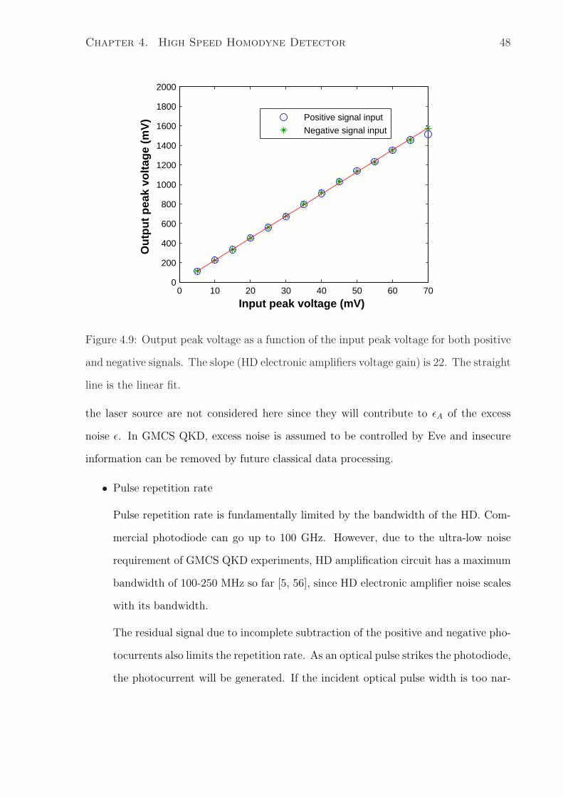
Chapter 4. High Speed Homodyne Detector 48
0 10 20 30 40 50 60 700
200
400
600
800
1000
1200
1400
1600
1800
2000
Input peak voltage (mV)
Ou
tpu
t p
eak
volt
age
(mV
) Positive signal input
Negative signal input
Figure 4.9: Output peak voltage as a function of the input peak voltage for both positive
and negative signals. The slope (HD electronic amplifiers voltage gain) is 22. The straight
line is the linear fit.
the laser source are not considered here since they will contribute to εA of the excess
noise ε. In GMCS QKD, excess noise is assumed to be controlled by Eve and insecure
information can be removed by future classical data processing.
• Pulse repetition rate
Pulse repetition rate is fundamentally limited by the bandwidth of the HD. Com-
mercial photodiode can go up to 100 GHz. However, due to the ultra-low noise
requirement of GMCS QKD experiments, HD amplification circuit has a maximum
bandwidth of 100-250 MHz so far [5, 56], since HD electronic amplifier noise scales
with its bandwidth.
The residual signal due to incomplete subtraction of the positive and negative pho-
tocurrents also limits the repetition rate. As an optical pulse strikes the photodiode,
the photocurrent will be generated. If the incident optical pulse width is too nar-

Chapter 4. High Speed Homodyne Detector 49
row, the photodiode may not be fast enough to respond and significant oscillations
will occur at the falling edge of the electrical pulse. Since two photodiodes are
employed in the HD circuit, in addition to photodiode intrinsic mismatch (such as
responsivity, and response time), different oscillation shapes from the two photodi-
odes will result in a considerable residual signal. Hence, wide optical pulse is used
to minimize the oscillations, however, this will limit the repetition rate.
• Pulse peak power and width
In the GMCS QKD, the photon number in each LO pulse is of the order of 107−109,
to ensure (a) the shot noise exceeds the electronic noise ; (2) the electronic circuit
is not saturated. Here I will discuss photodiode linearities in this required power
range.
The circuit and the setup shown in Fig. 4.10 are used in this test. Two types of
pulsed laser sources (shown in Table 4.2) running at 10 MHz repetition rate are
used to test photodiode linearity.
The experimental procedure is:
1. I send pulsed light (laser I or laser II) to only one photodiode by connecting
the switch with port 1 in Fig. 4.10 (b) and use an oscilloscope to measure
the electrical pulse peak voltage across the 10 Ohm resistor in Fig. 4.10 (a).
Optical power of the pulsed light is measured by connecting the switch with
port 3 in Fig. 4.10 (b).
2. Step 1 is repeated by sending pulsed light to the other photodiode when the
Table 4.2: Specifications of the two lasers used in photodiode linearity test
Laser number Type Pulse Width
I PriTel mode-lock femto second 0.7-1.2 ps
II CW modulated by amplitude modulator 50 ns

Chapter 4. High Speed Homodyne Detector 50
Figure 4.10: (a) Photodiode linearity test circuit. PD: photodiode; (b) Photodiode
linearity test setup. Laser I or II pulses are sent to one of the photodiodes. An oscilloscope
is used to measure the output peak voltage. PD: photodiode; Switch is connected with
port 1,2 to test the photodiode linearity, while connected with port 3 to measure the
optical power.
switch is connected with port 2.
Figure 4.7 (a) and (b) (in Section 4.3.2) show the oscilloscope waveforms of the
electrical output pulses with laser I or II as the source, respectively. Comparing
the two graphs, the electrical pulse peak voltage measured by the setup (Fig. 4.10
(a)) with laser I as a source is much higher than that with laser II. It is natural
because laser I has a narrow width (0.7-1.2 ps). Since the photodiode bandwidth is
2 GHz, the output pulse with a source of laser I has a width of �500 ps. The areas
(equivalent to energy) under two pulses are almost equal.
As shown in Fig. 4.11 (laser I) and Fig.4.12 (laser II), output electrical pulse peak
voltage across the 10 Ohm resistor (in Fig. 4.10 (a)) is plotted as a function of the
photon number in each optical pulse for both positive and negative photodiodes,
respectively.

Chapter 4. High Speed Homodyne Detector 51
0 5 10 15
x 107
0
50
100
150
200
250
Photon numbers per pulse
Ou
tpu
t p
uls
e am
plit
ud
e (m
V) Positive photodiode
Negative photodiode
Figure 4.11: Photodiode output peak voltage as a function of the photon number per
pulse with laser I (� 1 ps pulse width) as a source.
With laser I as a source (Fig.4.11), both photodiodes start to saturate when input
photon number/pulse exceeds 108. With laser II as a source (Fig. 4.12), photo-
diodes output voltage deviates � 4 % from their linear fits at up to 109 incident
photon per pulse. Power of laser II is limited to the non-tunable CW laser power.
One may find the photodiodes saturate at a lower optical input power level with
laser I as the source. In fact, the photodiodes are saturated by the high peak power
of laser I. At a photon number of 108 per incident pulse,
– Laser I: peak power = 108 � hν�0.7ps = 18 W
– Laser II: peak power = 108 � hν�50ns = 0.26 mW
To choose an appropriate laser source, one needs to guarantee that the photodiodes
are working in their linear regions to avoid saturation, which can be realized by
broadening the optical pulse.

Chapter 4. High Speed Homodyne Detector 52
0 2 4 6 8 10
x 108
0
5
10
15
20
25
Photon numbers per pulse
Ou
tpu
t p
uls
e am
plit
ud
e (m
V)
Positive photodiode
Negative photodiode
Figure 4.12: Photodiode output peak voltage as a function of the photon number per
pulse for laser II (� 50 ns pulse width) as a source
Considering different photodiode response functions, the linearity of the HD electronic
amplifier and that of the photodiode, a 50-ns-wide pulse with a rising/falling time of 15
ns generated by externally modulating CW laser at a repetition rate of 10 MHz is chosen
as the laser source.
4.3.5 Optical stability
The two beams between fiber coupler output ports and photodiodes (see Fig. 4.1) should
be well balanced in both lengths and intensities. However, owing to imperfect stability
of the optical setup, such as atmospheric turbulence and polarization dependent loss,
intensities of the two beams may drift. Here, I will give a simple example to show how
HD output is influenced by small intensity drifts of the two beams. Note that, the
optical source is chosen to be 50-ns-wide pulses generated by modulating CW light in
this analysis.
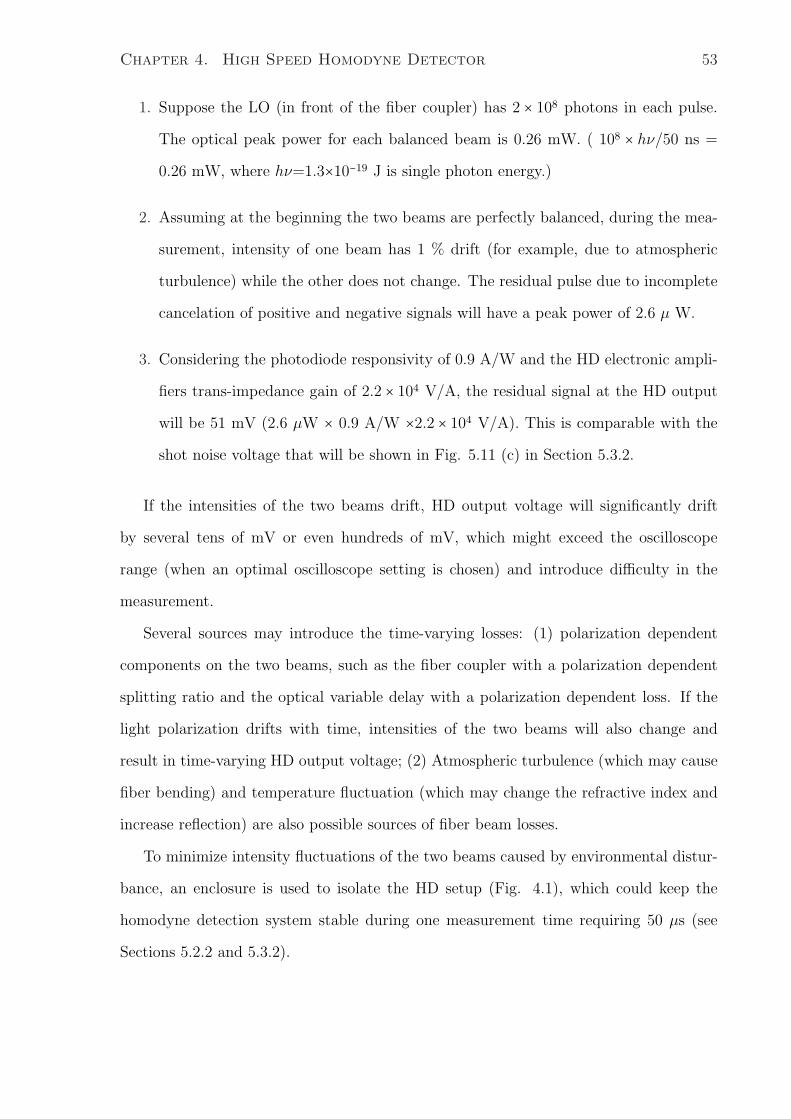
Chapter 4. High Speed Homodyne Detector 53
1. Suppose the LO (in front of the fiber coupler) has 2 � 108 photons in each pulse.
The optical peak power for each balanced beam is 0.26 mW. ( 108 � hν/50 ns =
0.26 mW, where hν=1.3�10−19 J is single photon energy.)
2. Assuming at the beginning the two beams are perfectly balanced, during the mea-
surement, intensity of one beam has 1 % drift (for example, due to atmospheric
turbulence) while the other does not change. The residual pulse due to incomplete
cancelation of positive and negative signals will have a peak power of 2.6 μ W.
3. Considering the photodiode responsivity of 0.9 A/W and the HD electronic ampli-
fiers trans-impedance gain of 2.2 � 104 V/A, the residual signal at the HD output
will be 51 mV (2.6 μW � 0.9 A/W �2.2 � 104 V/A). This is comparable with the
shot noise voltage that will be shown in Fig. 5.11 (c) in Section 5.3.2.
If the intensities of the two beams drift, HD output voltage will significantly drift
by several tens of mV or even hundreds of mV, which might exceed the oscilloscope
range (when an optimal oscilloscope setting is chosen) and introduce difficulty in the
measurement.
Several sources may introduce the time-varying losses: (1) polarization dependent
components on the two beams, such as the fiber coupler with a polarization dependent
splitting ratio and the optical variable delay with a polarization dependent loss. If the
light polarization drifts with time, intensities of the two beams will also change and
result in time-varying HD output voltage; (2) Atmospheric turbulence (which may cause
fiber bending) and temperature fluctuation (which may change the refractive index and
increase reflection) are also possible sources of fiber beam losses.
To minimize intensity fluctuations of the two beams caused by environmental distur-
bance, an enclosure is used to isolate the HD setup (Fig. 4.1), which could keep the
homodyne detection system stable during one measurement time requiring 50 μs (see
Sections 5.2.2 and 5.3.2).

Chapter 4. High Speed Homodyne Detector 54
In summary, several challenges in building a broad bandwidth and shot-noise limited
HD are discussed here. (1)HD electronic amplifiers and photodiodes should work in their
linear regions. (2) A proper laser source has to be chosen considering HD bandwidth,
components’ linearities and photodiode mismatch. (3) HD package should be carefully
designed to improve the system stability.
4.4 Summary
In this chapter, HD requirements for a high speed GMCS QKD system are proposed:
(1) a broad bandwidth of � 100 MHz; (2) 10 dB shot-noise-to-electronic-noise-ratio in
the time domain with a pulsed LO over a range of 108-109 photons/pulse. Based on the
HD circuit design from Prof. Lvovsky’s group, challenges in building a high speed HD
in the telecommunication wavelength region, from both electrical side to optical side,
are discussed. By choosing an optimal laser source, carefully stabilizing electrical and
optical components of the HD, and ensuring the linearities of photodiodes and electronic
amplifiers, we constructed a high speed HD required by GMCS QKD experiments.

Chapter 5
Performance of the Homodyne
Detector
In Chapter 4, requirements and challenges of constructing a shot-noise limited homodyne
detector (HD) for high speed GMCS QKD have been discussed. Based on limitations
from different photodiode response functions, linearities of photodiodes and HD electronic
amplifiers (see Section 4.3), I propose the HD electronic design and optical setup in
Section 4.2.
As discussed in Section 2.2.1, shot noise is proportional to the local oscillator (LO)
power and electronic noise is independent of the LO power. To prove the noise generated
by the HD is indeed the sum of shot noise and electronic noise, I need to verify that
the output noise variance, y, is related to the LO power, x, by an equation of the form,
y = ax + b where a and b are constants. On the other hand, as discussed in Section
3.3, shot-noise-to-electronic-noise-ratio ( shot noise variance divided by electronic noise
variance) at a specific LO power can be used to determine the magnitude of the electronic
noise (Nele, in shot noise unit) in QKD. Therefore, it is necessary to distinguish the two
noises by measuring the total noise of HD as a function of the LO power. In this chapter,
the HD performance is tested by this measurement.
55

Chapter 5. Performance of the Homodyne Detector 56
5.1 Experimental plan
To verify that the HD is shot-noise limited and to determine the shot-noise-to-electronic-
noise ratio, experiments are carried out as follows.
• Measure HD noise in the time domain (by an oscilloscope) and the frequency do-
main (by an RF spectrum analyzer) with different continuous wave (CW) local
oscillators.
• Measure HD noise in the time domain and in the frequency domain with different
pulsed local oscillators. The laser design has been discussed in Section 4.3.4.
Although a pulse-resolved shot-noise limited HD is our ultimate goal to implement
in a high speed GMCS QKD (see Section 2.1.2), it is technically challenging due to the
requirements of high subtraction (i.e. small residual signal), ultra-low noise and flat gain
over a broad bandwidth (see Section 2.2.2 and 4.3). As the first stage of verifying the
HD to be shot-noise limited, I test HD noise with CW LO, to reduce the residual signal
due to different response functions of the two photodiodes.
To illustrate feasibility of using this HD in future high speed GMCS QKD experi-
ments, HD noise is also tested with a pulsed LO and individual measurement of each
pulse will be shown. To have a thorough understanding of HD performance, measure-
ments are performed in both the time and the frequency domains. Finally, I will predict
the performance of a GMCS QKD experiment that uses our high speed HD.
5.2 Measurement with CW light
As discussed in Section 4.3.2, different response functions of two photodiodes of the HD
will cause incomplete subtraction of the positive and the negative photocurrents and
result in a residual signal (like in Fig. 4.6). To avoid the residual signal and have a

Chapter 5. Performance of the Homodyne Detector 57
Figure 5.1: Experimental setup with CW LO (NP Photonics). CW L: 1550 nm CW
fiber laser; VOA1-2: variable optical attenuators; LO: local oscillator; FC: 50:50 fiber
coupler; OVD: optical variable delay; PD: photodiodes; AMP: HD electronic amplifiers;
OSC: oscilloscope (Lecroy); RFSA: RF spectrum analyzer (HP 8564E); Dashed line box:
homodyne detector.
complete subtraction of the positive and negative signals, the total noise of HD is first
measured as a function of the CW LO power.
5.2.1 Experimental setup
In the setup shown in Fig 5.1, a CW laser (NP Photonics) is used as an LO and is
sent to one port of the fiber coupler. The other input port is left unconnected, and I
treat it as vacuum input by default. At the output, an oscilloscope and an RF spectrum
analyzer connected by an RF splitter are used to measure the HD noise. To eliminate
high frequency noises which are beyond the desired bandwidth 1, a low pass filter with
107 MHz bandwidth is applied at the HD output (it is omitted in our setup diagram). In
the subsequent discussions, LO power is defined to be the optical power measured before
it enters the fiber coupler.
1It may come from the electromagnetic oscillation of the feedback loop in the HD circuit. For thisparticular HD, the oscillation is over 600-800 MHz

Chapter 5. Performance of the Homodyne Detector 58
5.2.2 Noise measurement in the time domain
HD noise is measured as a function of the LO power in the time domain. The experimental
procedure is as follows.
1. The first step is to calibrate the system by balancing the two output paths of the
fiber coupler and their losses.
Figure 5.2: Calibration setup to get the balanced condition. Pulsed L: 1550 nm PriTel
pulsed femto second laser; VOA1-2: variable optical attenuators; LO: local oscillator; FC:
50:50 fiber coupler; OVD: optical variable delay; PD: photodiodes; AMP: HD electronic
amplifers; OSC: oscilloscope (Lecroy); RFSA: RF spectrum analyzer (HP 8564E); Dashed
line box: homodyne detector.
As shown in Fig. 5.2, a pulsed laser (PriTel femto second pulsed laser) is sent
to the fiber coupler as the LO. I change the delay time and attenuation until the
HD output voltage exhibits a minimum peak-to-peak value (shown in Fig. 4.6 in
Section 4.3.2). Most of the positive and negative electrical signals generated by
the two photodiodes cancel out under this condition (The degree of the subtraction
is quantified by the common mode rejection ratio, which will be discussed and
compared with other groups in Section 5.3.3).
2. I replace the pulsed laser by the CW source. With the setup shown in Fig. 5.1,
the output voltage is measured in a 50 μs window, with a sampling rate of 5 G

Chapter 5. Performance of the Homodyne Detector 59
samples/s. Fig. 5.3 shows the waveform of the oscilloscope (raw data). The total
noise of HD is obtained by calculating the voltage variance in this time window.
Figure 5.3: Oscilloscope graph for HD noise measurement at a CW LO power of 0.187
mW. Horizontal scale: 5 μs/div. Vertical scale: 2 mV/div.
3. With a different LO power, the measurement in Step 2 is repeated.
4. Oscilloscope noise is obtained by measuring output voltage variance in the absence
of any input to the oscilloscope channel.
Figure 5.4 shows HD noise and shot noise as a function of the LO power. Shot noise
is linearly dependent on the CW LO power. HD detector is 10-times shot-noise limited
at a CW LO power of � 2.8 mW. Note that, the oscilloscope noise is included in the
electronic noise (In fact, it is � 5% of the electronic noise).
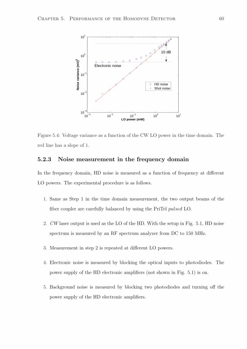
Chapter 5. Performance of the Homodyne Detector 60
10−3
10−2
10−1
100
101
10−3
10−2
10−1
100
101
LO power (mW)
No
ise
vari
ance
(m
V)2
HD noiseShot noise
Electronic noise
10 dB
Figure 5.4: Voltage variance as a function of the CW LO power in the time domain. The
red line has a slope of 1.
5.2.3 Noise measurement in the frequency domain
In the frequency domain, HD noise is measured as a function of frequency at different
LO powers. The experimental procedure is as follows.
1. Same as Step 1 in the time domain measurement, the two output beams of the
fiber coupler are carefully balanced by using the PriTel pulsed LO.
2. CW laser output is used as the LO of the HD. With the setup in Fig. 5.1, HD noise
spectrum is measured by an RF spectrum analyzer from DC to 150 MHz.
3. Measurement in step 2 is repeated at different LO powers.
4. Electronic noise is measured by blocking the optical inputs to photodiodes. The
power supply of the HD electronic amplifiers (not shown in Fig. 5.1) is on.
5. Background noise is measured by blocking two photodiodes and turning off the
power supply of the HD electronic amplifiers.

Chapter 5. Performance of the Homodyne Detector 61
Figure 5.5: RF spectrum analyzer background noise spectrum (lowest curve), HD elec-
tronic noise spectrum (second lowest curve) and HD noise spectra at CW LO powers of
6.4400, 4.1400, 2.5380, 1.5960, 1.0180, 0.6460, 0.4140, 0.2528,0.1592,0.1014,0.0640,0.0410
and 0.0252 mW (from the highest to the third lowest curve). Resolution bandwidth: 1
MHz
HD noise power as a function of the frequency at different LO powers is shown in Fig.
5.5. It indicates that (1) the HD has a bandwidth of � 100 MHz (when power drops by
3 dB); (2) the noise power increases as the LO power increases.
Noise power is calculated by integrating the area under each curve. To eliminate the
strong noise centered at DC (shown in Fig. 5.6, might be contributed by pink noise,
instrument noise and small incomplete subtraction of positive and negative signals), the
spectral noise power (in Fig. 5.5) is integrated from 5 MHz to 110 MHz, since the noise
below 5 MHz is not mainly contributed by HD electronic noise and shot noise.
Figure 5.7 shows the shot noise is linearly dependent on the LO power in the frequency
domain. HD is 10-times shot-noise limited at an LO power of � 2.6 mW, which has a
good agreement with that in the time domain, which is 2.8 mW. Here, the RF spectrum

Chapter 5. Performance of the Homodyne Detector 62
0 2 4 6 8 10−70
−60
−50
−40
−30
−20
−10
0
Frequency (MHz)
No
ise
po
wer
(d
Bm
/MH
z)
Figure 5.6: Noise spectrum from DC to 10 MHz at an LO power of 0.3 mW. Resolution
bandwidth: 1 MHz
analyzer noise (6% of the electronic noise) is included in the electronic noise.
5.3 Measurement with pulsed light
To measure electric field quadratures of individual pulse in GMCS QKD, a broad band-
width and shot-noise limited HD working with pulsed LO is required. Performance of
the HD with pulsed LO will be discussed in this section.
5.3.1 Pulsed laser source
As discussed in Section 4.3.4, I choose 50-ns-wide (with 15 ns rising/falling time) pulsed
laser by externally modulating CW light with an amplitude modulator controlled by a
function generator at a repetition rate of 10 MHz.
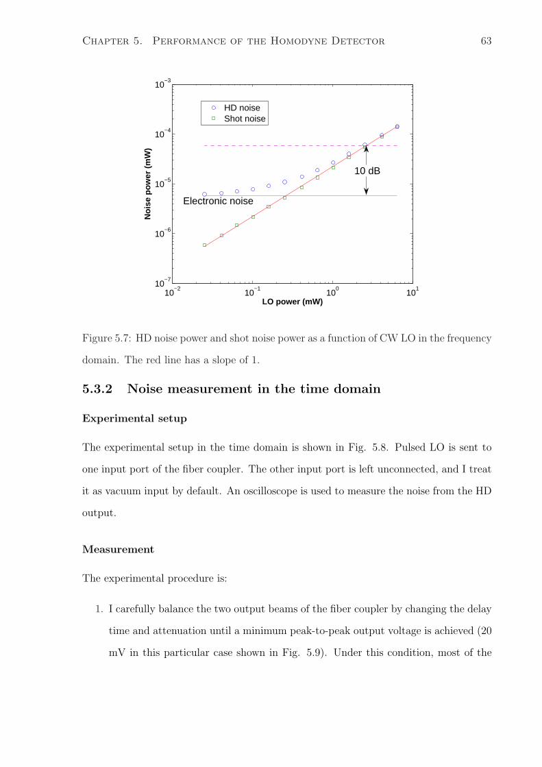
Chapter 5. Performance of the Homodyne Detector 63
10−2
10−1
100
101
10−7
10−6
10−5
10−4
10−3
LO power (mW)
No
ise
po
wer
(m
W)
HD noiseShot noise
10 dB
Electronic noise
Figure 5.7: HD noise power and shot noise power as a function of CW LO in the frequency
domain. The red line has a slope of 1.
5.3.2 Noise measurement in the time domain
Experimental setup
The experimental setup in the time domain is shown in Fig. 5.8. Pulsed LO is sent to
one input port of the fiber coupler. The other input port is left unconnected, and I treat
it as vacuum input by default. An oscilloscope is used to measure the noise from the HD
output.
Measurement
The experimental procedure is:
1. I carefully balance the two output beams of the fiber coupler by changing the delay
time and attenuation until a minimum peak-to-peak output voltage is achieved (20
mV in this particular case shown in Fig. 5.9). Under this condition, most of the

Chapter 5. Performance of the Homodyne Detector 64
Figure 5.8: Experimental setup of HD noise measurement in the time domain. CW L:
1550 nm CW fiber laser; VOA1-2: variable optical attenuators; LO: local oscillator; FC:
50:50 fiber coupler; OVD: optical variable delay; PD: photodiodes; AMP: HD electronic
amplifiers; OSC: oscilloscope (Lecroy); Dashed line box: homodyne detector.
Figure 5.9: HD output waveform under the balanced condition at an LO power of 0.786
mW. Horizontal scale: 50 ns/div. Vertical scale: 50 mV/div. The square box on this
graph indicates one cycle.
positive and negative signals cancel out. To quantify how good the subtraction is,
the common mode rejection ratio (CMRR) can be estimated.

Chapter 5. Performance of the Homodyne Detector 65
CMRR is used to characterize the subtraction ability of the HD while it rejects
DC and preserves AC of the two input signals. Ideally, one expects the HD output
Vo = A�V1 − V2�, where V1 and V2 (voltage or current) are input signals. However,
for a practical HD, the output Vo can be described as
Vo = A1�V1 − V2� + A2
2�V1 + V2� (5.1)
where A1 is the rejection mode gain and A2 is the common mode gain (typically
smaller than A1). The CMRR is defined as
CMRR = 10 log10�A1
A2
�2 = 20 log10 �A1
A2
�. (5.2)
If the input and output signals are represented in power (i.e. V1, V2, and Vo are
power inputs and output), CMRR is defined as 10 log10 �A1
A2�.
To estimate CMRR experimentally, several approximations are made.
• If only one photodiode is illuminated and the other is blocked (i.e. V1 � 0, V2 =0), output Vo1 is
Vo1 = A1V1 + A2
2V1 � A1V1 (5.3)
where A1 � A2 is assumed considering that the rejection mode gain is far
larger than the common mode gain for a balanced receiver.
• When both photodiodes are both illuminated (i.e. V1 = V2), output Vo2 is
Vo2 = A1�V1 − V2� + A2
2�V1 + V2� � A2
22V1 = A2V1 (5.4)
where V1 = V2 (i.e. perfectly balanced signal inputs) is assumed.
If V1 is the same in the two cases, ratio of �A1
A2� can be obtained from �Vo1
Vo2�.
Under this particular condition in Fig. 5.9, Vo1 = 15 V 2 and Vo2 � 20 mV (by read-
ing the peak-to-peak voltage in Fig. 5.9). CMRR can be obtained by 20 log10 � 150.02 �
2It is estimated from the average optical power shining on one photodiode 0.786�2 = 0.393 mW, pulseduty cycle = 50 %, photodiode responsivity η = 0.90 A/W, and the HD circuit gain GTI =2.2� 104 V/A.Output HD voltage when only one photodiode is illuminated will be 0.393 mW/50% �η �GTI = 15 V

Chapter 5. Performance of the Homodyne Detector 66
= 58 dB. Note that, Vo1 cannot be measured directly by blocking one photodiode,
since this high voltage will saturate the HD circuit.
2. 50 μs is chosen as one frame to measure the HD output voltages (shown in Fig.
5.10), while there are 500 pulse cycles in each frame. The main reason to make
measurement within a very short time is to avoid the intensity drift introduced by
the system instability and environmental influences (see Section 4.3.5).
3. Step 2 is repeated under different LO powers.
4. Oscilloscope noise is measured in the absence of signal input.
Figure 5.10: One measurement frame at an LO power of 0.4 mW. Horizontal scale: 10
mV/div, Vertical scale: 5 μs/div.
Data processing
The following data processing is applied to the original waveform in Fig. 5.10.

Chapter 5. Performance of the Homodyne Detector 67
1. I break each frame into 500 segments of equal length, named S�i�.�i = 1,2, ...500)
Each segment S�i� corresponds to 100 ns, which is the period of the pulsed LO.
These segments, having the same time span, are folded onto each other, as shown
in Fig. 5.11 (a).
Figure 5.11: Data processing procedure (LO = 0.77 mW). (a) 500 original curves (one
frame) S; (b) Background curve (i.e., the average curve) of S; (c) 500 processed curves
(one frame) T .

Chapter 5. Performance of the Homodyne Detector 68
2. As shown in Fig. 5.11 (a), S�i� exhibits a DC offset in which the voltages are not
zero at the non-pulsed region (0-15 ns and 70-100 ns), caused by the HD circuit and
residual signals (peaks at 20 ns and 65 ns) due to different response functions of
the two photodiode (see Section 4.3.2). I calculate the average voltage of all curves
in S�i� as the background (shown in Fig. 5.11 (b) ). Processed pulses are obtained
by subtracting the background from S�i�, named T �i� (shown in Fig. 5.11 (c)).
3. For each processed curve T �i�, noise is calculated by adding all voltages within the
pulsed region (from 15 ns to 70 ns), named N�i�, by a similar approach in Ref. [5].
4. Variance of N�i� at each LO power is obtained as the HD noise variance.
5. The oscilloscope noise is measured in the same way in the absence of input to the
oscilloscope channel.
Results
HD noise variance and shot noise variance are plotted as a function of the LO power in
Fig. 5.12. Shot noise is linearly dependent on the LO power. The HD is 10-times shot-
noise limited at an LO power of 5.4�108 photons/pulse (0.7 mW) in the time domain.
Here, the oscilloscope noise (13 % of the electronic noise) is included in the electronic
noise. The results with pulsed LO should not be directly compared to those obtained
with CW LO, because we adopt a data processing technique that average noises within
a 55 ns time window in each cycle.
In GMCS QKD, Bob needs to measure the electric field quadrature of each signal
pulse individually. In the test of shot noise when vacuum is sent to the signal port, one
needs to verify that each pulse yields only one quadrature value. As a simple way to
check, the correlation coefficient (CC) between adjacent pulses is evaluated. At a specific
LO power of 0.77 mW, I perform HD noise measurement 10 times and combine those
noises to obtain a larger sample size NLarge�j��j = 1,2, ...,5000�. Two arrays X�k� and

Chapter 5. Performance of the Homodyne Detector 69
10−3
10−2
10−1
100
101
10−3
10−2
10−1
100
LO power (mW)
No
ise
vari
ance
(V
2 )
HD noiseShot noise
Electronic noise
10 dB
Figure 5.12: HD noise variance and shot noise variance as a function of the pulsed LO
power in the time domain. The red line has a slope of 1.
Y �k� (k = 1,2, ...,4900) are assigned by
X�k� = NLarge�k�, Y �k� = NLarge�k +m��m = 0,1,2, ...,10�. (5.5)
CC between X and Y is defined as
CC = E�XY � −E�X�E�Y ��E�X2� −E2�X��E�Y 2� −E2�Y � . (5.6)
Figure 5.13 depicts the CC between two measured quadrature sequences X and Y
at an LO power of 0.77 mW as a function of m. The value of CC when m = 1 is 0.034,
which is comparable with other HDs developed by Ref. [5] (0.04) and Ref. [57] (0.07).
The small correlation between two adjacent pulses could be contributed by HD electronic
noise correlation. Fig. 5.14 shows a direct representation of the sets X and Y when m =
1. X and Y are very independent. These results demonstrate the realization of individual
measurement of each pulse.

Chapter 5. Performance of the Homodyne Detector 70
0 2 4 6 8 10−0.2
0
0.2
0.4
0.6
0.8
1
1.2
m
Co
rrel
atio
n c
oef
fici
ent
Figure 5.13: Correlation coefficient between nth (X) and n +mth (Y) pulses at an LO
power of 0.77 mW
HD noise measurements in the time domain with pulsed LO can be used to predict the
future high speed QKD performance. Using the GMCS QKD experimental parameters
in Ref. [1] (shown in Table 5.1), under the “realistic model”, GMCS QKD key rates as
a function of the transmission distance with this new constructed high-speed HD and
existing low-speed HD are simulated in Fig. 5.15. Note that, parameters used in this
simulation are based on a low-speed GMCS QKD system and may not be valid for a
high-speed experiment. This simulation is used to predict the order of magnitude of the
key rate of a GMCS QKD experiment using our high-speed HD. In this simulation, an
LO photon number of 108 per pulse, at which the low-speed HD is shot-noise limited (see
Fig. 3.5 in Section 3.3), is selected for a low speed GMCS QKD system. For comparison,
the same LO level is chosen for a high speed GMCS QKD system. The key rate when our
high-speed HD shows 10-times shot-noise limited (at an LO of 5.4�108 photons/pulse) is
also simulated for a high speed GMCS QKD experiment.

Chapter 5. Performance of the Homodyne Detector 71
−3 −2 −1 0 1 2 3−3
−2
−1
0
1
2
3
X (V)
Y (
V)
Figure 5.14: Quadrature value of nth pulse X�n� and that of n+1 pulse Y �n� =X�n+1�at an LO power of 0.77 mW
Key rates can be increased by about 2 orders of magnitude by employing our high
speed HD in the GMCS QKD experiment (comparing the blue solid, the green dashed-
dotted curve with the red dashed curve). This is due to the 10 MHz repetition rate
permitted by 100 MHz broad bandwidth of the HD. This simulation results show GMCS
QKD key rate with the high-speed HD is expected to achieve a few Mbits/s over a short
distance (0-15 km), comparable to the world-fastest key rates of 1.02 Mbits/s achieved
Table 5.1: Parameters in the key rate simulation (given in Ref. [1]). Here we assume εA
and Nleak are the same for high-speed and low-speed GMCS QKD experiments.
VA η χ εA Nleak
16.9 0.44 2.25 0.056 0.02

Chapter 5. Performance of the Homodyne Detector 72
0 5 10 15 20 25 3010
0
101
102
103
104
105
106
107
Distance (km)
Key
rat
e (b
it/s
)
High speed (10 MHz, LO = 5.4*108 photons/pulse)
High speed (10 MHz, LO = 108 photons/pulse)
Low speed (100 kHz, LO = 108 photons/pulse)
Figure 5.15: Key rate simulation as a function of the transmission distance with a high-
speed HD (running at 10 MHz repetition rate) and a low-speed HD (running at 100 kHz
repetition rate)
by Ref. [4] over 20 km and 1.34 Mbits/s achieved by Ref. [46] over 10 km using single
photon QKD protocols. If one looks at the blue solid and green dashed-dotted curves
obtained by using the fast HD in the simulation, a stronger LO power can be used to
achieve a higher key rate.
In summary, this fast HD has been demonstrated to be 10-times shot-noise limited at
a pulsed LO level of 5.4 � 108 photons/pulse in the time domain. Meanwhile, individual
measurements of each pulse are demonstrated. This HD meets the requirements discussed
in Section 4.1 and is expected to improve the key rate by 2 orders of magnitude in future
GMCS QKD experiments.

Chapter 5. Performance of the Homodyne Detector 73
5.3.3 Noise measurement in the frequency domain
Experimental setup
The experimental setup in the frequency domain is shown in Fig. 5.16. An RF spectrum
analyzer (HP 8564E) is used to measure the HD output noise.
Figure 5.16: Experimental setup in the frequency domain. CW L: 1550 nm CW fiber
laser; VOA1-2: variable optical attenuators; AM: amplitude modulator; PC: polarization
controller; LO: local oscillator; FC: 50:50 fiber coupler; OVD: optical variable delay; PD:
photodiode; AMP: HD electronic amplifers; RFSA: RF spectrum analyzer (HP 8564E);
Dashed line box: homodyne detector.
Measurement
The experimental procedure is:
1. Same as Step 1 in the time domain measurement in Section 5.3.2 , the system has
to be calibrated to a well-balanced condition.
2. Noise power is measured from DC to 100 MHz first (shown in Fig. 5.17). There
are peaks at DC, 10 MHz, and higher harmonics of the repetition rate. The DC
component is mainly due to the pink noise and DC offset (see the time domain
data processing step 2 in Section 5.3.2). Those 10 MHz harmonic frequencies are
mainly contributed by residual signal power due to the incomplete subtraction of
the positive and negative signals.

Chapter 5. Performance of the Homodyne Detector 74
0 20 40 60 80 100−70
−60
−50
−40
−30
−20
−10
0
10
Frequency (MHz)
No
ise
po
wer
(d
Bm
/100
kH
z)
Figure 5.17: Noise spectrum at an LO power of 0.786 mW. Frequency range: DC to 100
MHz. Resolution bandwidth: 100 kHz.
3. CMRR measurement in the frequency domain
Direct measurement of CMRR in the frequency domain can be obtained by measur-
ing the noise power at the repetition rate (10 MHz) when (1) both two photodiodes
have incident optical powers (shown in Fig. 5.18 (a), this peak at 10 MHz is min-
imized by carefully balancing the two channels); and (2) only one photodiode has
incident optical power while the other photodiode is blocked (shown in Fig. 5.18
(b)). Note that, CMRR can not be directly measured at high LO powers. Ow-
ing to the huge trans-impedance gain (2.2�104 V/A, see Section 4.3.3), the HD is
easily saturated when only one photodiode is illuminated. In this experiment, the
maximum LO to avoid saturation is 49.4μW and I choose an LO power of 24.56μW
in the particular measurement shown in Fig. 5.18.
4. Noise spectrum measurement
In Fig. 5.17, the peaks at 10 MHz and its harmonics are not mainly contributed
by the shot noise. To measure shot noise, a frequency span from 5 MHz to 6 MHz

Chapter 5. Performance of the Homodyne Detector 75
Figure 5.18: Noise spectrum at an LO power of 24.56 μW when (a)two photodiodes are
illuminated; (b)one photodiode is blocked. Resolution bandwidth: 100 kHz
(far from the peaks) is chosen. This noise measurement is repeated at different LO
powers.
5. Spectrum analyzer noise is measured in the same way of step 4 in the absence of
input signal.

Chapter 5. Performance of the Homodyne Detector 76
Figure 5.19: Noise spectra at different LO powers. Frequency span: 5 to 6 MHz. Reso-
lution bandwidth: 10 kHz. LO powers are 0.0029, 0.0072, 0.0142, 0.0292, 0.0458, 0.0721,
0.1136, 0.1784, 0.2920, 0.4580, 0.7180, 1.1340, 1.7760, 2.9200 mW from the lowest curve
to the highest curve, respectively.
Results
From Fig. 5.18, the CMRR is obtained to be 54.33 dB by finding the ratio of powers at
10 MHz of the two cases, which is better than 45 dB in Ref. [5] measured at low LO
powers (the exact power is not given).
Noise spectra at different LO powers are shown in Fig.5.19. I integrate the spectral
noise under each curve over this 1 MHz frequency span. In Fig. 5.20, the noise power
is plotted as a function of the LO power. Shot noise is linearly dependent on the LO
power. The HD is 10-times shot-noise limited at an LO power of 1.54 mW (1.2�109
photons/pulse). The noise of the RF spectrum analyzer (6% of the electronic noise) is
included in the electronic noise.

Chapter 5. Performance of the Homodyne Detector 77
10−3
10−2
10−1
100
101
10−9
10−8
10−7
10−6
10−5
LO power (mW)
No
ise
po
wer
(m
W)
HD noiseShot noise
Electronic noise
10 dB
Figure 5.20: Noise power as a function of the LO power in the frequency domain. The
red line has a slope of 1.
With pulsed LO, HD noise measurements are performed in the time and the frequency
domains. In the time domain, to remove DC offset and residual signals, we performed
data processing (see Section 5.3.2), which applies a window of 55 ns in the time domain.
In the frequency domain, a 1-MHz frequency span is chosen to measure the spectral
noise. Different schemes employed in the two domains make it difficult to compare the
shot-noise-to-electronic-noise ratio with the pulsed LO.
5.4 Conclusions and discussions
In this chapter,the HD performance is tested by measuring HD noise as a function of
the LO power in both time and frequency domains. The main results are summarized as
follows.
1. The HD has a bandwidth of � 100 MHz. It is of the same order as the broad-

Chapter 5. Performance of the Homodyne Detector 78
est bandwidth HDs working at non-telecommunication wavelengths reported by
other groups [5, 30-32]. In the telecommunication wavelength region, no group has
reported HDs with broader bandwidths for use in quantum measurements.
2. With CW LO, shot noise is verified to be linearly dependent on the LO power in
the time/frequency domains. Shot noise can be above electronic noise by 10 dB at
2.6-2.8 mW LO powers. Shot-noise-to-electronic-noise-ratios are in good agreement
in the two domains. The measurement with CW light is just a preliminary test of
the HD and will not be used in future real GMCS QKD experiments.
3. With pulsed LO running at 10 MHz, shot noise is tested to be linearly dependent
on the LO power in the time/frequency domains. By using this HD, future high
speed GMCS QKD is able to operate at a repetition rate of 10 MHz, which is 1-2
orders of magnitude higher than current reported GMCS QKD systems [1, 43]. The
expected key generation rate (a few Mbits/s) is of the same order of magnitude as
the world-fastest single photon QKD experiments [4, 46].
In summary, for the first time, a �100 MHz broad bandwidth HD in the telecommu-
nication wavelength region is reported. At a pulse repetition rate of 10 MHz, a 10-times
shot-noise limited HD performance can be achieved at an LO of 5.4 � 108 photons per
pulse. With this high-speed HD, future GMCS QKD key rate is expected to achieve a
few Mbits/s over a short distance.
In future, HD can be improved in the following ways.
1. Photodiode pair that is fabricated under the same condition [51] can be used to
eliminate the residual signal due to different photodiode response functions. This
will be helpful to improve the subtraction of the HD and achieve a better shot-
noise-to-electronic-noise-ratio by using a higher LO power without saturating the
HD. With a well-matched photodiode pair, we expect to use an LO pulse containing

Chapter 5. Performance of the Homodyne Detector 79
1010 − 1011 photons, which might improve the current shot-noise-to-electronic-noise
ratio by 1-2 orders of magnitude. 3
2. Electronic noise of a HD will contribute to the excess noise and reduce key rate. In
future, to reduce electronic noise, we could cool the amplifiers and the photodiode.
Furthermore, we can choose amplifiers with lower gains, since the electronic noise
scales with gain (see Section 4.3.1). To ensure the shot noise can be detected, a
stronger LO power will be required, because HD output is proportional to EL (see
Section 2.2.1). To increase the LO power without saturating the HD circuit, the
problem of the residual signal due to different photodiode response functions should
be solved first.
3. Instead of the data processing in Section 5.3.2, filtering DC component by a high
pass filter and harmonic frequencies at laser repetition rate by notch filters can be
used to remove the residual signal and HD circuit DC offset (shown in Fig. 5.11 (b)),
which is suggested by Prof. Lvovsky. This will not improve the HD performance
directly but will avoid the trouble of implementing the data processing.
4. HDs based on integrated circuits (IC) have an advantage over those based on dis-
crete circuits. The main advantages of an IC are: (1) components are built in
a compact way and the parasitic impedance can be reduced; (2) a good quality
control and repeatable performance can be achieved. However, developing the HD
based on IC is also challenging: (1) designing the interface between commercial
photodiodes and IC might be difficult; (2) a custom IC may lack flexibility for
corrections and incremental improvements. Although there are challenges, it still
3This can be roughly estimated from Fig. 4.9 in Section 4.3.3 and Fig. 5.11 in Section 5.3.2 (c). Thelinear region of the HD electronic amplifier is at least 2V obtained from Fig. 4.9. If the residual signalis neglected using a well-matched photodiode pair, shot noise magnitude can be 2V without saturatingthe HD, which is 2 orders of magnitude greater than 20mV in Fig. 5.11 (c) in Section 5.3.2 at an LO of6�108 photons/pulse (0.77 mW). Therefore, we expect to use 6� 1010 photons/pulse without saturatingthe HD by employing a perfectly matched photodiode pair.

Chapter 5. Performance of the Homodyne Detector 80
might be a promising direction for further improving HD performance.

Chapter 6
Conclusion and Future Work
6.1 Significance and contribution
Pulse-resolved balanced homodyne detection has attracted a great attention for its appli-
cation in quantum information and quantum optics [73]. A broadband and pulse-resolved
HD in the telecommunication wavelength region used in GMCS QKD has been developed
and tested in this thesis. Table 6.1 compares the performance of our HD and the HD
from Hirano’s group, which has the broadest bandwidth in quantum optics and quan-
tum information applications. The bandwidth of our HD has achieved the same order
of magnitude as that in Ref. [5]. HD subtraction performance (indicated by CMRR) of
our HD is 9 dB higher (Note that, authors of Ref. [5] measured the CMRR using a low
LO power but they did not specify their LO power. The comparison might not be made
with the same LO power).
In Ref. [5], squeezed state is measured in both time and frequency domains. During
their measurement, pulses are identical when a particular phase between LO and signal is
fixed. Therefore, measurement in the time domain is not the only way to characterize the
squeezed state. Measuring the noise in the frequency domain can also used to determine
the uncertainty of squeezed states.
81
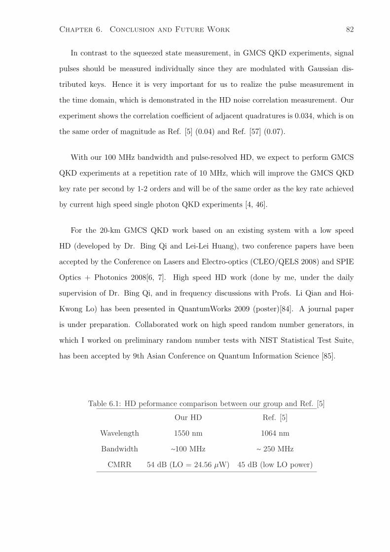
Chapter 6. Conclusion and Future Work 82
In contrast to the squeezed state measurement, in GMCS QKD experiments, signal
pulses should be measured individually since they are modulated with Gaussian dis-
tributed keys. Hence it is very important for us to realize the pulse measurement in
the time domain, which is demonstrated in the HD noise correlation measurement. Our
experiment shows the correlation coefficient of adjacent quadratures is 0.034, which is on
the same order of magnitude as Ref. [5] (0.04) and Ref. [57] (0.07).
With our 100 MHz bandwidth and pulse-resolved HD, we expect to perform GMCS
QKD experiments at a repetition rate of 10 MHz, which will improve the GMCS QKD
key rate per second by 1-2 orders and will be of the same order as the key rate achieved
by current high speed single photon QKD experiments [4, 46].
For the 20-km GMCS QKD work based on an existing system with a low speed
HD (developed by Dr. Bing Qi and Lei-Lei Huang), two conference papers have been
accepted by the Conference on Lasers and Electro-optics (CLEO/QELS 2008) and SPIE
Optics + Photonics 2008[6, 7]. High speed HD work (done by me, under the daily
supervision of Dr. Bing Qi, and in frequency discussions with Profs. Li Qian and Hoi-
Kwong Lo) has been presented in QuantumWorks 2009 (poster)[84]. A journal paper
is under preparation. Collaborated work on high speed random number generators, in
which I worked on preliminary random number tests with NIST Statistical Test Suite,
has been accepted by 9th Asian Conference on Quantum Information Science [85].
Table 6.1: HD peformance comparison between our group and Ref. [5]
Our HD Ref. [5]
Wavelength 1550 nm 1064 nm
Bandwidth �100 MHz � 250 MHz
CMRR 54 dB (LO = 24.56 μW) 45 dB (low LO power)

Chapter 6. Conclusion and Future Work 83
6.2 Future work
In this thesis, we developed a high speed shot-noise limited HD in the telecommunication
wavelength region. There are a few practical problems we can try to solve, such as
different photodiode response functions. For a fully telecommunication fiber-based high
speed GMCS QKD, an optical system and a control system should be investigated in
future.
1. Different photodiode response functions
In high speed HD construction, a very practical problem is the residual signal
due to different response functions of the photodiodes. To overcome this problem,
there are a few feasible methods. First, a well-matched photodiode pair that two
photodiodes are fabricated under idenetical condition can be used to minimize the
residual signal. Second, a HD based on one photodiode can be studied, which we
call a self-differencing scheme.
This self-differencing scheme is first introduced by Ref. [86] to construct high speed
single photon detectors. If we use this idea in HD, the schematic is shown in Fig.
6.1,
(a) The signal and local oscillator interfere at the left 50/50 optical splitter.
(b) We can introduce a time delay between the resulting two pulses to separate
them in the time domain.
(c) The two pulses are recombined in the right 50/50 optical splitter. Now we
should expect two separate optical pulses (shown as the red pulses). We call
them pulse 1 and pulse 2.
(d) We use one photodiode to detect both optical pulses, converting them into
two electrical pulses (shown as the lower right two blue pulses).

Chapter 6. Conclusion and Future Work 84
Figure 6.1: A self-differencing scheme in homodyne detection. Red pulses are optical
pulses and blue pulses are electrical pulses.
(e) The two electric pulses are then splitted into four electric pulses by the electric
splitter. We call them pulse 1’, 2’, 1”, 2”.
(f) We introduce another time delay which is identical to the optical delay in-
troduced in Step (b) by an electric delay. The purpose is to align the second
pulse in the upper path (pulse 2’) and the first pulse in the lower path (pulse
1”) in the time domain.
(g) We perform a subtraction between the two paths. We expect to receive a large
negative pulse (pulse 1’) and a large positive pulse (pulse 2”). In the middle
of these two strong pulses we may observe the desired result (pulse 1” - pulse
2’).
(h) Output signal will be amplified by electronic amplifiers (not shown).
The advantages of this scheme are
(a) All the components (except the electronic amplifiers) are passive with a high

Chapter 6. Conclusion and Future Work 85
speed and low noise.
(b) We use only one photodiode. Therefore we can eliminate most of photodiode
mismatch discussed in Section 4.3.2.
(c) Most compenents are commercial and the implementation is simple.
But there are still a few challenges in this scheme,
(a) All the passive devices should not introduce much distortion to the shapes of
electrical pulses.
(b) With a huge gain of subsequent electronic amplifier, the pulses 1’ and 2” will
saturate the electronic amplifiers. One possible solution is to let electronic
amplifiers work in a gating mode (i.e., it is operating when the incoming signal
is the subtraction of pulses 1” and 2’). An alternative method is to carefully
choose the repetition rate to overlap pulse 1’ and pulse 2” from the previous
cycle in the time domain. This will also double the effective repetition rate.
(c) The loss of this system has to be calibrated carefully.
This novel self-differencing scheme is worth trying to solve the photodiode mismatch
problem.
2. Local oscillator power
The optimal LO power has to be investigated systematically. The excess noises
from Bob’s system have two sources: HD electronic noise Nele and noise associate
with the leakage photon from LO to signal Nleak. To suppress Nele, a strong LO
should be chosen in order to improve the shot-noise-to-electronic-noise ratio. How-
ever, controlling the leakage photon from the LO beam to the signal beam is more
technically challenging with a strong LO. Therefore, a tradeoff between the two
noises has to be made when we choose a proper LO power.

Chapter 6. Conclusion and Future Work 86
3. Optical scheme
Time-multiplexing [43], time-frequency-multiplexing [66] and polarization-frequency-
multiplexing [1] schemes are existing techniques to suppress the excess noise due to
leakage interference of LO and leakage from LO to signal [1, 43, 44]. It is necessary
to conduct more research to select an optimal scheme for future high speed GMCS
QKD.
To achieve a high sped GMCS QKD system in real time operation, improving the
speed of the data acquisition is still in demand. To control the system excess noise
induced by the environment, the system stability should be investigated. In parallel
with these development, new algorithms, which aim at achieving farther communication
distance and higher secret key generation rates based on more efficient reconciliation are
meaningful research directions.

Bibliography
[1] B. Qi, L.-L. Huang, L. Qian, and H.-K. Lo, “Experimental study on Gaussian-
modulated coherent states quantum key distribution over standard telecom fiber,”
Phys. Rev. A 76, 052 323 (2007).
[2] Y. Zhao, B. Qi, X. Ma, H.-K. Lo, and L. Qian, “Simulation and Implementation of
Decoy State Quantum Key Distribution over 60km Telecom Fiber,” Proceedings of
IEEE International Symposium on Information Theory 2006 p. 2094 (2006).
[3] H. Takesue, S. W. Nam, Q. Zhang, R. H. Hadfield, T. Honjo, K. Tamaki, and Y. Ya-
mamoto, “Quantum key distribution over 40 dB channel loss using superconducting
single photon detectors,” Nature photonics 1, 343 (2007).
[4] A. R. Dixon, Z. L. Yuan, J. F. Dynes, A. W. Sharpe, and A. J. Shields, “Gigahertz
decoy quantum key distribution with 1 Megabit/s secure key rate,” Opt. Express
16, 18 790 (2008).
[5] R. Okubo, M. Hirano, Y. Zhang, and T. Hirano, “Pulsed-resolved measurement
of quadrature phase amplitudes of squeezed pulse trains at a repetition rate of 76
MHz,” Opt. Lett. 33, 1458 (2008).
[6] B. Qi, L.-L. Huang, Y.-M. Chi, L.Qian, and H.-K. Lo, “Gaussian-modulated coher-
ent state quantum key distribution experiment over 20km telecommunication fiber,”
in SPIE Optics + Photonics 2008 San Diego, CA, Aug 10-14 .
87

Bibliography 88
[7] B. Qi, L.-L. Huang, Y.-M. Chi, L.Qian, and H.-K. Lo, “Excess Noise Control in
Gaussian-Modulated Coherent State Quantum Key Distribution System,” in Oral
presentation at the Conference on Lasers and Electro-optics (CLEO/QELS 2008),
San Jose, CA, May 4-9, 2008, paper QWE1 .
[8] H.-K. Lo and Y. Zhao, “Quantum cryptography,” Encyclopedia of Complexity and
System Science 8, 7265 (2009).
[9] N. Gisin, G. Ribordy, W. Tittel, and H. Zbinden, “Quantum cryptography,” Reviews
of Modern Physics 74, 145 (2002).
[10] R. L. Rivest, A. Shamir, and L. M. Adleman, “A method for obtaining digital
signatures and public-key cryptosystems,” Communications of the ACM 21, 128
(1978).
[11] P. W. Shor, “Algorithms for Quantum Computation: Discrete Logarithms and Fac-
toring,” Proc. 35th Annual Symp. on Foundations of Computer Science p. 124
(1994).
[12] G. Vernam, “Cipher Printing Telegraph Systems For Secret Wire and Radio Tele-
graphic Communications,” J. Am. Inst. Ele. Eng. 45, 109 (1926).
[13] C. Shannon, “One-Time Pads For Secure Communication In Ubiquitous,” Bell Sys-
tem Tech. J. 28, 656 (1949).
[14] C. Bennett and G. Brassard, “Quantum cryptography: Public key distribution and
coin tossing,” Proceedings of IEEE International Conference on computers, systems
and signal processing p. 175 (1984).
[15] A. K. Ekert, “Quantum cryptography based on Bells theorem,” Phys. Rev. Lett.
67, 661 (1991).
Bibliography 89
[16] W. Wootters and W. Zurek, “A Single Quantum Cannot be Cloned,” Nature 299,
802 (1982).
[17] D. Dieks, “Communication by EPR devices,” Phys. Rev. A 92, 271 (1982).
[18] V. Buzek and M. Hillery, “Quantum cloning,” Physics world 14, 25 (2001).
[19] F. Grosshans, G. V. Assche, J. Wenger, R. Brouri, N. J. Cerf, and P. Grangier,
“Quantum key distribution using Gaussian-modulated coherent states,” Nature 421,
238 (2003).
[20] D. Mayers, “Unconditional security in quantum cryptography,” J. ACM 48, 351
(2001).
[21] H.-K. Lo and H. F. Chau, “Unconditional security of quantum key distribution over
arbitrary long distances,” Science 283, 2050 (1999).
[22] P. W. Shor and J. Preskill, “Simple proof of security of the BB84 Quantum key
distribution protocol,” Phys. Rev. Lett. 85, 441 (2000).
[23] D. Gottesman, H.-K. Lo, N. Lutkenhaus, and J. Preskill, “Security of quantum key
distribution with imperfect devices,” Quantum Inf. Comput. p. 325 (2004).
[24] C. H. Bennett, F. Bessette, G. Brassard, L. Salvail, and J. Smolin, “Experimental
quantum cryptography,” J. of Cryptography 5, 3 (1992).
[25] P.D.Townsend, J.G.Rarity, and P. Tapster, “Single photon interference in 10 km
long optical fiber interferometer,” Electron. Lett. 29, 634 (1993).
[26] A. Muller, J. Breguet, and N. Gesin, “Experimental demonstratino of quantum cryp-
tography using polarized photons in optical fiber over more than 1 km,” Europhys.
Lett. 23, 383 (1993).

Bibliography 90
[27] D. S. Naik, C. G. Peterson, A. G. White, A. J. Berglund, and P. G. Kwiat, “Entan-
gled State Quantum Cryptography: Eavesdropping on the Ekert Protocol,” Phys.
Rev. Lett. p. 4733 (2000).
[28] F. Grosshans and P. Grangier, “Continuous Variable Quantum Cryptography Using
Coherent States,” Phys. Rev. Lett. 88, 057 902 (2002).
[29] Z. Yuan, B. E. Kardynal, R. M. Stevenson, A. J. Shields, C. J. Lobo, K. Cooper,
N. S. Beattie, D. A. Ritchie, and M. Pepper, “Electrically Driven Single-Photon
Source,” Science 295, 102 (2001).
[30] J. McKeever, A. Boca, A. D. Boozer, R. Miller, J. R. Buck, A. Kuzmich, and H. J.
Kimble, “Deterministic Generation of Single Photons from One Atom Trapped in a
Cavity,” Science 303, 1992 (2004).
[31] T. Babinec, B. M. Hausmann, M. Khan, Y. Zhang, J. Maze, P. R. Hemmer,
and M. Loncar, “A Bright Single Photon Source Based on a Diamond Nanowire,”
arXiv:0908.0233 (2009).
[32] N. Lutkenhaus, “Security against individual attacks for realistic quantum key dis-
tribution,” Phys. Rev. A 61, 052 304 (2000).
[33] W. Y. Hwang, “Quantum Key Distribution with High Loss: Toward Global Secure
Communication,” Phys. Rev. Lett. 91, 057 901 (2003).
[34] H.-K. Lo, X. Ma, and K. Chen, “Decoy State Quantum Key Distribution,” Phys.
Rev. Lett. 94, 230 504 (2005).
[35] X. Ma, B. Qi, Y. Zhao, and H.-K. Lo, “Practical decoy state for quantum key
distribution,” Phys. Rev. A 72, 012 326 (2005).
[36] Y. Zhao, B. Qi, X. Ma, H.-K. Lo, and L. Qian, “Experimental Quantum Key Dis-
tribution with Decoy States,” Phys. Rev. Lett. 94, 072 502 (2006).

Bibliography 91
[37] X.-B. Wang, “Beating the Photon-Number-Splitting Attack in Practical Quantum
Cryptography,” Phys. Rev. A 94, 230 503 (2005).
[38] M. Koashi, “Unconditional Security of Coherent-State Quantum Key Distribution
with a Strong Phase-Reference Pulse,” Phys. Rev. Lett. 93, 120 501 (2004).
[39] J. Lodewyck, T. Debuisschert, R. Tualle-Brouri, and P. Grangier, “Controlling ex-
cess noise in fiber-optics continuous-variable quantum key distribution,” Phys. Rev.
A 72, 050 303.
[40] M. Legre, H. Zbinden, and N. Gisin, “Implementation of continuous variable quan-
tum cryptography in optical fibres using a go & return configuration,” Quant. Info.
Compu. 6, 326 (2006).
[41] R. Namiki and T. Hirano, “Practical Limitation for Continuous-Variable Quantum
Cryptography using Coherent States,” Phys. Rev. Lett. 92, 117 901 (2004).
[42] M. Heid and N. Lutkenhaus, “Security of coherent-state quantum cryptography in
the presence of Gaussian noise,” Phys. Rev. A 76, 022 313 (2007).
[43] J. Lodewyck, M. Bloch, R. Garca-Patrn, S. Fossier, E. Karpov, E. Diamanti, T. De-
buisschert, N. J. Cerf, R. Tualle-Brouri, S. W. McLaughlin, and P. Grangier, “Quan-
tum key distribution over 25 km with an all-fiber continuous-variable system,” Phys.
Rev. A 76, 042 305 (2007).
[44] S. Fossier, E. Diamanti, T. Debuisschert, R. Tualle-Brouri, and P. Grangier, “Im-
provement of continuous-variable quantum key distribution systems by using optical
preamplifiers,” arXiv:0812.4314 (2008).
[45] V.Scarani, H. Bechmann-Pasquinucci, N. J. Cerf, M. Dusek, N. Lutkenhaus, and
M. Peev, “The Security of Practical Quantum Key Distribution,” arXiv:0802.4155v2
.

Bibliography 92
[46] Q. Zhang, H. Takesue, T. Honjo, K. Wen, T. Hirohata, M. Suyama, Y. Takiguchi,
H. Kamada, Y. Tokura, O. Tadanaga, Y. Nishida, M. Asobe, and Y. Yamamoto,
“Megabits secure key rate quantum key distribution,” New. J. Phys. 11, 045 010
(2009).
[47] A. Zavatta, M. Bellini, P. L. Ramazza, F. Marin, and F. T. Arecchi, “Time-domain
analysis of quantum states of light: noise characterization and homodyne tomogra-
phy,” J. Opt. Soc. Am. B 19, 189 (2002).
[48] H. Hansen, T. Aichele, C. Hettich, P. Lodahl, A. I. Lvovsky, J. Mlynek, and
S. Schiller, “An ultra-sensitive pulsed balanced homodyne detector: Application
to time-domain quantum measurements,” Opt. Lett. 26, 1430 (2001).
[49] H. Yuen and V. W. S. Chan, “Noise in homodyne and heterodyne detection,” Opt.
Lett. 8, 177 (1983).
[50] T. Okoshi, “Heterodyne and coherent optical fiber communications - Recent
progress,” IEEE Trans. on Microwave Theory and Technologies p. 1138 (2009).
[51] Http://www.chipsat.com/.
[52] Http://www.eoc-inc.com/.
[53] C. Zhang, Y. Mori, K. Igarashi, K. Katoh, and K. Kikuchi, “Ultrafast operation of
digital coherent receivers using their time-division demultiplexing function,” J. of
Lightw. Tech. 27, 224 (2009).
[54] G. Li, “Recent advances in coherent optical communication,” Advances in optics
and photonics 1, 279 (2009).
[55] T. Hirano, H. Yamanaka, M. Ashikaga, T. Konishi, and R. Namiki, “Quantum
cryptography using pulsed homodyne detection,” Phys. Rev. A 68, 042 331 (2003).
Bibliography 93
[56] J. Appel, D. Hoffman, E. Figueroa, and A. I. Lvovsky, “Electronic noise in optical
homodyne tomography,” Phys. Rev. A 75, 035 802 (2007).
[57] O. Haderka, V. Michalek, V. Urbasek, and M. Jezek, “Fast time-domain balanced
homodyne detection of light,” Appl. Opt. 48, 2884 (2009).
[58] N. J. Cerf and P. Grangier, “From quantum cloning to quantum key distribution
with continuous variable: a review,” J. Opt. Soc. Am. B 24, 324 (2007).
[59] C. Shannon, “A Mathematical Theory of Communication,” Bell syst. Tech. J. 27,
379 (1948).
[60] F. Grosshans and N. J. Cerf, “Continuous-Variable Quantum Cryptography is Secure
against Non-Gaussian Attacks,” Phys. Rev. Lett. 92, 047 905 (2004).
[61] M. Navascues, F. Grosshans, and A. Acin, “Optimality of Gaussian Attacks in
Continuous-Variable Quantum Cryptography,” Phys. Rev. Lett. 97, 190 502 (2006).
[62] R. Garcia-Patron and N. J. Cerf, “Unconditional Optimality of Gaussian Attacks
against Continuous-Variable Quantum Key Distribution,” Phys. Rev. Lett. 97,
190 503 (2006).
[63] R. Renner and J. I. Cirac, “A de Finetti representation theorem for infi-
nite dimensional quantum systems and applications to quantum cryptography,”
arXiv:0809.2243 (2008).
[64] A. Leverrier, E. Karpov, P. Grangier, and N. J. Cerf, “Unconditional security of
continuous-variable quantum key distribution,” arXiv:0809.2252v2 (2008).
[65] Y.-B. Zhao, Z.-F. Han, and G.-C. Guo, “Apply current exponential de Finetti the-
orem to realistic quantum key distribution,” arXiv:0809.2683v2 (2008).

Bibliography 94
[66] S. Fossier, E. Diamanti, T. Debuisschert, A. Villing, R. Tualle-Brouri, and P. Grang-
ier, “Field test of a continuous-variable quantum key distribution prototype,”
arXiv:0812.3292 (2008).
[67] C. Weedbrook, A. M. Lance, W. P. Bowen, T. Symul, T. C. Ralph, and P. K. Lam,
“Quantum Cryptography Without Switching,” Phys. Rev. Lett. 93, 170 504 (2004).
[68] C. Weedbrook, A. M. Lance, W. P. Bowen, T. Symul, T. C. Ralph, and P. K. Lam,
“Coherent-state quantum key distribution without random basis switching,” Phys.
Rev. A 73, 022 316 (2006).
[69] A. M. Lance, T. Symul, V. Sharma, C. Weedbrook, T. C. Ralph, and P. K. Lam,
“No-Switching Quantum Key Distribution Using Broadband Modulated Coherent
Light,” Phys. Rev. A 95, 180 503 (2005).
[70] G. Abbas, V. Chan, and T. Yee, “Local-oscillator excess-noise suppression for ho-
modyne and heterodyne detection,” Opt. Lett. 8, 419 (1983).
[71] H. A. Haus, in Electromegnetic noise and quantum optical measurement pp. 281–288
(2000).
[72] H. Bachor and T. C. Ralph, in A guide to experiment in Quantum optics (2nd
edition) pp. 206–208 (2004).
[73] A. I. Lvovsky and M. G. Raymer, “Continuous-variable optical quantum state to-
mograpy,” arXiv:quant-ph/0511044v2 (2008).
[74] A. Zavatta, S. Viciani, and M. Bellini, “Quantum-to-Classical Transition with Single-
Photon-Added Coherent States of Light,” Science 306, 660 (2003).
[75] M. Silva, Q. Xu, S. Agnolini, P. Gallion, and F. Mendieta, “Homodyne detection
for quantum key distribution: an alternative to photon counting in BB84 protocol,”
hotonics North Conference Proceeding, Quebec City, Canada, June (2006).

Bibliography 95
[76] D. T. Smithey, M. Beck, M. G. Raymer, and A. Faridani, “Measurement of the
Wigner distribution and the density matrix of a light mode using optical homodyne
tomography: Application to squeezed states and the vacuum,” Phys. Rev. Lett. 70,
1244 (1993).
[77] N. Jain, S.-H. Youn, and A. I. Lvovsky, “Quantum tomography of the single photon
state generated by down conversion in a periodically poled KTP crystal,” Quantum
communication, measurement and computing (QCMC) p. 201 (2008).
[78] M. Mehmet, S. Steinlechner, T. Eberle, H. Vahlbruch, A. Thuring, K. Danzmann,
and R. Schnabel, “Observation of continuous-wave squeezed light at 1550 nm,”
arXiv:0902.0670 (2009).
[79] M. Hillery, “Quantum cryptography with squeezed states,” Phys. Rev. A 61, 022 309
(2000).
[80] D. Stucki, N. Walenta, F. Vannel, R. T. Thew, N. Gisin, H. Zbinden, S. Gray, C. R.
Towery, and S. Ten, “High rate, long-distance quantum key distribution over 250
km of ultra low loss fibres,” New. J. Phys. 11, 075 003 (2009).
[81] S. R. Huisman, N. Jain, S. A. Babichev, F. Vewinger, A.-N. Zhang, S.-H. Youn,
and A. I. Lvovsky, “Instant single-photon Fock state tomography,” arXiv:0902.0670
(2009).
[82] Vasilescu, in Electronic noise and interfering signals: principles and applications p.
433 (2005).
[83] L. T. Gnecco, in The design of shielded enclosures: cost-effective methods to prevent
EMI (2000).

Bibliography 96
[84] Y.-M. Chi, L. Tian, B. Qi, L. Qian, and H.-K. Lo, “High-Speed Homodyne Detector
for Gaussian-Modulated Coherent State Quantum Key Distribution,” in Quantum-
Works 2009 poster .
[85] B. Qi, Y.-M. Chi, L. Qian, and H.-K. Lo, “High speed random number genera-
tion based on measuring phase noise of a single mode diode laser,” in 9th Asian
Conference on Quantum Information Science .
[86] Z. L. Yuan, B. E. Kardynal, A. W. Sharpe, and A. J. Shields, “High speed single
photon detection in the near-infrared,” Appl. Phys. Lett. 91, 041 114 (2007).


![arXiv:1809.00818v1 [quant-ph] 4 Sep 2018 · Homodyne tomography with homodyne-like detection Stefano Olivares,1,2 Alessia Allevi,3,4, Giovanni Caiazzo,3 Matteo G. A. Paris,1,2 and](https://img.pdfslide.net/doc/110x75/5eae5d295913200fa42c38a4/arxiv180900818v1-quant-ph-4-sep-2018-homodyne-tomography-with-homodyne-like.jpg)