Embed Size (px)
Citation preview
Journal of the Mechanics and Physics of Solids 112 (2018) 291–317
Contents lists available at ScienceDirect
Journal of the Mechanics and Physics of Solids
journal homepage: www.elsevier.com/locate/jmps
High strain-rate soft material characterization via inertial cavitation
Jonathan B. Estrada a , Carlos Barajas b , David L. Henann a , Eric Johnsen
b , Christian Franck
a , ∗
a School of Engineering, Brown University, Providence, RI, United States b Mechanical Engineering Department,University of Michigan, Ann Arbor, MI, United States
a r t i c l e i n f o
Article history:
Received 29 August 2017
Revised 5 November 2017
Accepted 13 December 2017
Available online 14 December 2017
Keywords:
Dynamics
Viscoelastic material
Mechanical testing
Inertial cavitation
High strain rate
a b s t r a c t
Mechanical characterization of soft materials at high strain-rates is challenging due to their
high compliance, slow wave speeds, and non-linear viscoelasticity. Yet, knowledge of their
material behavior is paramount across a spectrum of biological and engineering applica-
tions from minimizing tissue damage in ultrasound and laser surgeries to diagnosing and
mitigating impact injuries. To address this significant experimental hurdle and the need to
accurately measure the viscoelastic properties of soft materials at high strain-rates (10 3 –
10 8 s −1 ), we present a minimally invasive, local 3D microrheology technique based on in-
ertial microcavitation. By combining high-speed time-lapse imaging with an appropriate
theoretical cavitation framework, we demonstrate that this technique has the capability to
accurately determine the general viscoelastic material properties of soft matter as com-
pliant as a few kilopascals. Similar to commercial characterization algorithms, we provide
the user with significant flexibility in evaluating several constitutive laws to determine the
most appropriate physical model for the material under investigation. Given its straightfor-
ward implementation into most current microscopy setups, we anticipate that this tech-
nique can be easily adopted by anyone interested in characterizing soft material properties
at high loading rates including hydrogels, tissues and various polymeric specimens.
© 2017 Elsevier Ltd. All rights reserved.
1. Introduction
The ability to accurately predict how mechanical forces affect the response of tissues and cells crucially depends upon un-
derstanding the constitutive response of the underlying tissue. Accurate mechanical characterization of soft matter, including
hydrogels and tissues, relies on the availability of appropriate experimental techniques that can address the highly compliant
nature and the length- and time-dependent characteristics of these materials. Classical tension-compression experiments as
well as plate-and-cone rheometry provide a good approach for estimating bulk material properties ( Hu et al., 2011; Johnson
et al., 2004; Marra et al., 20 01; Muniz and Geuskens, 20 01; Zhao et al., 2010 ) yet they only provide information on material
behavior at macroscopic length scales. Alternatively, small-scale techniques such as microindentation, nanoindentation, and
atomic force microscopy allow for interrogation of the local, rather than bulk elastic ( Ebenstein and Pruitt, 2004; Hu et al.,
2010 ), and poro/viscoelastic properties ( Hu et al., 2011; Kalcioglu et al., 2012 ). This makes these techniques attractive for
∗ Corresponding author.
E-mail address: [email protected] (C. Franck).
https://doi.org/10.1016/j.jmps.2017.12.006
0022-5096/© 2017 Elsevier Ltd. All rights reserved.
292 J.B. Estrada et al. / Journal of the Mechanics and Physics of Solids 112 (2018) 291–317
probing tissue properties at the size scale of cells and tissues. However, due to the intrinsic inhomogeneous loading con-
ditions, accurate determination of material properties beyond the linear elastic regime requires more sophisticated contact
mechanics models to be employed beyond the classical Hertz and Johnson–Kendall–Roberts (JKR) theories, which are not
always readily available ( Lin et al., 2009; Style et al., 2013 ).
Recently, several promising in situ microrheology approaches including optical trapping ( Svoboda and Block, 1994 ), con-
focal rheology ( Dutta et al., 2013; Kollmannsberger and Fabry, 2007 ), and pressure-induced cavitation ( Kundu and Crosby,
2009; Zimberlin and Crosby, 2010; Zimberlin et al., 2007 ) have emerged for providing new detail of the intrinsic 3D me-
chanical properties inside polymeric materials. In particular, pressure-induced cavitation rheology as pioneered by Crosby
and coworkers is a powerful, compact testing platform for determining the local mechanical properties of soft materials and
tissues across material length scales by measuring the cavitation bubble radius ( Kundu and Crosby, 2009; Zimberlin and
Crosby, 2010; Zimberlin et al., 2007 ). In this approach, air or immiscible liquid injected via a syringe pump reaches a critical
pressure, which either induces cavitation or fracture depending on material composition and stiffness.
While measurements via these techniques have contributed much to our current understanding of the mechanical, or
constitutive, properties of hydrogels, tissues, and soft matter, almost all of them have focused on the quasi-equilibrium re-
sponse of the material at low- to medium-level strain-rates ( 10 −4 − 10 2 s −1 ). Extension of the mentioned techniques to
faster loading rates is often challenged by limitations in the employed hardware or necessity for more sophisticated theo-
retical frameworks ( Klopp and Clifton, 1985 ) accounting for internal wave propagation and inertial effects.
With increasing demand for understanding soft matter behavior at higher loading rates (i.e., strain-rates > 10 3 s −1 ) mo-
tivated by applications in laser- and ultrasound-based surgical procedures ( Maxwell et al., 2009; Venugopalan et al., 2002;
Xu et al., 2007 ) and impact injuries ( Meaney and Smith, 2011; Nyein et al., 2011; Ramasamy et al., 2010 ), significant demand
exists for experimental techniques capable of physically characterizing the tissue response at those rates. For example, injury
prediction during traumatic brain injuries ( Bar-Kochba et al., 2016 ) and collateral tissue damage estimates during lithotripsy
procedures ( Mancia et al., 2017 ) require a quantitative understanding of the relevant tissue at strain-rates in excess
of 10 3 s −1 .
Established techniques for traditional high strain-rate mechanical characterization of inorganic and less compliant mate-
rials, including Split–Hopkinson (Kolsky) bar and pressure-shear testing, have been met with challenges when used for soft
materials due to the high compliance, low impedance, and slow shear wave speeds in these materials ( Chen and Song, 2010 ).
These challenges are compounded further by the lack of readily available theoretical frameworks that allow rapid interpre-
tation of the dynamic, inertia-dominated data at hand.
The purpose of this paper is to overcome these significant challenges and to address the need for a high strain-rate
characterization technique. We present a robust, minimally-intrusive, local microrheology approach for characterizing the
material constitutive properties at high (10 3 s −1 ) to ultra-high (10 8 s −1 ) strain-rates. Using a spatially-focused pulsed laser
we are able to generate inertial cavitation bubbles in a variety of hydrogels of varying stiffness at pre-defined depths of field.
Analogous to the quasistatic cavitation rheology, the bubble dynamics within the interrogated material are a direct function
of the material mechanical properties. Recording the spatiotemporally resolved bubble dynamics via high-speed videog-
raphy, one can determine the constitutive material model via a standard least squares fitting approach to an appropriate
theoretical-numerical cavitation modeling framework, which we developed for this particular purpose. Our mathematical
inertial cavitation framework is built upon previously developed single-bubble cavitation studies ( Akhatov et al., 2001; Ep-
stein and Keller, 1972; Flynn, 1975; Keller and Kolodner, 1956; Keller and Miksis, 1980; Nigmatulin et al., 1981; Prosperetti
et al., 1988; Prosperetti and Lezzi, 1986 ) in order to provide accurate estimates of the non-linear, finite deformation vis-
coelastic material properties of the tissue or hydrogel.
To demonstrate the capability and validity of this new inertial microcavitation-based high strain-rate material characteri-
zation technique, we mechanically characterize soft and stiff polyacrylamide gels as a benchmark case. Lastly, we show that
once the material properties are obtained, one can use the theoretical framework to predict the spatiotemporal evolution of
cavitation stresses and strains, which should be of significant interest in understanding the physical forces experienced by
tissues in laser eye surgery ( Cherian and Rau, 2008 ), ultrasound surgical methods in cancer treatment ( Parsons et al., 2006 ),
lithotripsy ( Bailey et al., 2003 ), and impact deformations in the brain ( Nyein et al., 2011; Sarntinoranont, 2012 ).
1.1. Overview of Inertial Microcavitation-based high strain-rate Rheometry
Similar to other material characterization techniques, Inertial Microcavitation high strain-rate Rheometry (IMR) correlates
the evolution of the bubble pressure and the stress field in the material with the resulting kinematics, namely the change in
bubble radius over time, which is recorded via high-speed videography ( Fig. 1 A). In essence, one can think of this technique
as a force-controlled tribology method, in which a certain amount of energy is added into the material system to start
the cavitation process as shown in Figs. 1 B and 2 . Since cavitation initiation requires the creation of a pressure differential
across the bubble wall, various means have been devised to accomplish it, and the associated underlying physics need to be
properly reflected in the governing equations used to model the cavitation process.
In this study, single bubble inertial cavitation is generated via single pulses of a frequency-doubled Q-switched Nd:YAG
532 nm laser as shown in Fig. 1 A. Shortly after bubble nucleation, luminescence occurs, signifying initial plasma formation
and chemical reactions at the laser focal point ( Fig. 2 ). As the bubble rapidly expands, plasma recombines into the gas
inside the bubble and the system reaches thermodynamic, though not mechanical, equilibrium. While bubble dynamics are

J.B. Estrada et al. / Journal of the Mechanics and Physics of Solids 112 (2018) 291–317 293
A B
Nd:YAG532 nm
6ns, 1-10 mJ
Beam Expander
Alignment Diode0.8 mW, 634 nm
VisionPhantom
v2511
TI-EclipseInverted
Microscope
HalogenLamp
Δt = 3.7 µs
µm
Rmax
200
Objective
Hydrogel **
laser pulse
Fig. 1. Experimental setup and schematic of inertial microcavitation rheometry. (A) A single 6 ns, Q-switched 532 nm Nd:YAG laser pulse of 1–10 mJ
passes through a beam expander to fill the back aperture of an objective mounted into an inverted TI-Eclipse microscope, and (inset, star) converges into
a cylindrical hydrogel sample. Bright-field illumination is supplied by a condensed halogen lamp. (B) Bubble growth, collapse, and subsequent oscillation
are imaged using a Phantom v2511 high speed camera (Vision Research, Wayne, NJ). Image size 512 ×128 px, filmed at 270,0 0 0 fps. Scale bar, 200 μm.
6 ns, 1-10 mJ
532
nm Normalized Time, t* 2t
0* 4 6
1
0.5
Nor
mal
ized
Rad
ius,
R*
00
t0*t* >>
R0
σrr(t
0)
t0*t* =
pb(t
0)
Rmax
2γ
Rmax
µG
Material model
Com
plex
gro
wth
phy
sics
Ela
stic
ity D
omin
ates
ViscosityDominates
MechanicalEquilibrium
Fig. 2. Schematic of the timeline after inertial cavitation bubble nucleation. After initial plasma formation, bubble growth is caused by plasma recombina-
tion and vapor and non-condensible gas volume expansion, and reaches thermodynamic equilibrium ( t ∗0 ). Modeling of the bubble dynamics is begun at the
time of maximum bubble radius, t ∗0 . The peak bubble size builds large elastic stresses in the surrounding material, which drive primary bubble collapse.
Later, lower-amplitude bubble oscillation is dominated by material viscous effects, finally reaching mechanical equilibrium.
recorded experimentally during and after growth ( Fig. 1 B), we do not consider the laser-induced process of material rupture
in our numerical model as the physics during inertial cavitation are relatively complex and, at present, only incompletely
understood ( Akhatov et al., 2001 ).
Instead, we construct our theoretical framework beginning at the time of the peak bubble radius. Fig. 2 shows a
schematic of the initial ( t = t 0 , R = R max ) and reference ( t � t 0 , R = R 0 ) states of the model. At t = t 0 , the surrounding hy-
drogel material is out of dynamic equilibrium, with surface tension and material stress greater than the internal bubble
pressure. At later times t � t 0 , the material is assumed to be in mechanical equilibrium with the gas inside the bubble. A

294 J.B. Estrada et al. / Journal of the Mechanics and Physics of Solids 112 (2018) 291–317
widely-accepted, general approach for modeling the contents of the bubble inside hydrogel- or tissue-based soft matter sys-
tems is to treat the bubble contents as a two-phase mixture of condensible water vapor and non-condensible gas (for which
condensation rate is much slower than the timescales of the bubble oscillations) ( Fujikawa and Akamatsu, 1980 ).
While Fig. 2 provides a schematic of the typical oscillatory single bubble cavitation behavior, it is important to note that
the amplitude, frequency and decay of the bubble radius oscillations are directly affected by the underlying viscoelastic
material properties. Connecting the characteristic oscillation to the appropriate material response is the determining goal of
the presented IMR method. If the material behaves viscoelastically, the initially large elastic stress determines the rate of
primary collapse, while the overall decay envelope is dominated by viscous dissipation.
The remainder of this paper is organized as follows. In Section 2 , the theoretical framework for inertial microcavitation
rheometry is presented. Experimental details and setup are described in Section 3 . Experimental and numerical results for
water and two tested polyacrylamide concentrations are presented in Section 4 . Finally, we discuss the stress and strain
evolution during microcavitation as well as important limitations of the technique in Sections 5 and 6 .
2. Theoretical cavitation framework
In this section, we discuss the theoretical framework utilized to model the cavitation process, which draws upon the
extensive literature on single-bubble cavitation in a fluid ( Akhatov et al., 2001; Epstein and Keller, 1972; Flynn, 1975; Fu-
jikawa and Akamatsu, 1980; Keller and Kolodner, 1956; Keller and Miksis, 1980; Nigmatulin et al., 1981; Prosperetti, 1991;
Prosperetti et al., 1988; Prosperetti and Lezzi, 1986 ). The mathematical formulation involves several key assumptions. First,
since bubble oscillations remain largely spherical over the course of the cavitation process ( Fig. 1 B), we assume that the
motion of the bubble, its contents, and the surroundings are spherically symmetric. Second, given the high water content of
many biological tissues and hydrogels and the small time-scales characterizing the cavitation process, we assume no water
flux with respect to the surrounding material, i.e., the surroundings remain undrained. As a result of the undrained ideal-
ization, we also assume that the surrounding material is nearly incompressible. More specifically, we follow the approach
of Keller and Miksis (1980) , which corrects an ideally incompressible description of the surrounding material in the region
near the bubble ( r ∼ o ( R ) where R is the radius of the bubble) by incorporating the material’s finite sound speed in the
description of the far-field ( r ∼ o ( ct ) where c is the longitudinal wave speed of the surroundings) in order to account for
energy transfer through acoustic radiation. The Keller-Miksis formulation is accurate to first order in the ratio of the bubble
wall velocity to the longitudinal wave speed of the surroundings, ˙ R /c ( Prosperetti and Lezzi, 1986 ). Finally, due to a lack of
time-resolved measurements very close to the collapse of the bubble, we model the dynamics of the bubble contents using
a low Mach number approximation ( Yang and Church, 2005 ), which neglects high Mach number effects inside the bubble
( Akhatov et al., 2001 ).
2.1. Surrounding material
Denote the equilibrium radius of the spherical bubble as R 0 and the referential radial coordinate in the surrounding
material as r 0 , where r 0 is measured from the center of the bubble. The surrounding material is identified by material points
R 0 < r 0 < ∞ . Then, the time-dependent radius of the bubble wall during the process of growth and collapse is denoted as
R ( t ), and the surrounding material undergoes large deformations in which material points r 0 are mapped to deformed points
r ( r 0 , t ). The spatial description of the radial velocity field is then denoted as v ( r, t ). 1
2.1.1. Near-field
We first discuss the response of the surrounding material in the vicinity of the bubble, i.e., r ∼ o ( R ). In this region, the
finite sound speed of the material is unimportant, and therefore, the surrounding material may be idealized as incompress-
ible. Under the assumptions of spherical symmetry and near-field incompressibility, the balance of mass requires that
∂v
∂r +
2 v
r = 0 . (1)
Integrating (1) and expressing the radial velocity at the bubble wall in terms of the bubble radius, i.e., v (R, t) = ˙ R (t) , allows
us to establish the following relationship between the radial velocity v ( r, t ), the bubble radius R ( t ), and the spatial radial
coordinate r :
v = ˙ R R 2
r 2 . (2)
Next, denote the Cauchy stress tensor as σ( r, t ) and decompose σ( r, t ) into its hydrostatic pressure p ( r, t ) and its deviatoric
part s ( r, t ) as σ = s − pI . For the case of spherical symmetry, the radial component of the momentum balance equations in
1 Regarding notation, we develop the theoretical cavitation framework using the spatial description, in which ∂ ( • )/ ∂ t and ∂ ( • )/ ∂ r denote the spatial time
derivative and spatial radial gradient, respectively. For quantities that are a function of time alone, such as the deformed bubble-wall radius R ( t ), we denote
the time derivative by a superposed dot, i.e., ˙ R (t) .

J.B. Estrada et al. / Journal of the Mechanics and Physics of Solids 112 (2018) 291–317 295
the absence of external body forces requires that
ρ
(
∂v
∂t + v
∂v
∂r
)
= −∂ p
∂r +
∂s rr ∂r
+ 2
r ( s rr − s θθ ) , (3)
where ρ is the constant mass density of the surrounding material and s rr ( r, t ) and s θθ ( r, t ) are the radial and hoop com-
ponents of the deviatoric stress tensor s ( r, t ). In a Rayleigh–Plesset-like approach, which assumes that the incompressible
idealization applies in the surroundings for all r > R , one may substitute (2) in (3) , invoke an appropriate constitutive model
for the deviatoric response of the material, and integrate over r from r = R to r → ∞ to obtain an ordinary differential equa-
tion (ODE) for the time evolution of the bubble radius R ( t ). However, assuming ideal incompressibility for all r > R precludes
accounting for energy transfer through radial acoustic emission from the bubble to the far field – an effect that has a quan-
titative impact on the bubble dynamics, especially for large bubble-radius oscillation amplitudes ( Keller and Miksis, 1980 ).
In order to incorporate the effects of slight compressibility and the associated finite wave speed of the material, Keller and
Kolodner (1956) , Epstein and Keller (1972) , and Keller and Miksis (1980) proposed an approximate formulation combining
the ideally-incompressible near-field behavior with far-field, linearized wave propagation. In the present work, we follow a
similar path.
2.1.2. Far-field
In the far-field (i.e., r �R ), the strains induced by growth and collapse of the bubble decay rapidly. Therefore, deforma-
tions may be considered small, and the governing equations may be linearized. In this spatial region, the dominant physics
are acoustic wave propagation. Since the ideally-incompressible assumption discussed above implies an infinite wave speed,
it is incompatible with this physics, and we must relax the incompressible idealization to account for the finite wave speed
of the material. Accordingly, we assume that the linearized bulk modulus of the material is finite but still much greater
than the linearized shear modulus and model the material as linear elastic with a constant longitudinal wave speed c that
is dominated by the bulk modulus. The radial component of the Navier equations of linear elasticity for the case of spherical
symmetry may be recast in terms of the radial velocity field as
c 2 ∂
∂r
[
1
r 2 ∂
∂r (r 2 v )
]
= ∂ 2 v
∂t 2 . (4)
The solution of (4) for the far-field radial velocity field may be conveniently written in terms of a potential function φ( r, t )
as v = ∂φ/ ∂r , so that (4) may be expressed in terms of φ( r, t ) as
c 2 (
∂ 2 φ
∂r 2 +
2
r
∂φ
∂r
)
= ∂ 2 φ
∂t 2 , (5)
which is simply the spherical version of the one-dimensional wave equation. A solution for the potential function φ( r, t ),
which is consistent with (5) , is
φ = 1
r f
(
t −r
c
)
, (6)
where f is an arbitrary function. Eq. (6) physically represents acoustic wave propagation from the bubble outward. Of course,
the general solution of (5) also includes an additional term similar in form to (6) but with the argument (t + r/c) , which
physically represents acoustic wave propagation from the far-field inward. This physics can be important in certain cases
– for example, in ultrasonic cavitation driven by far-field acoustic excitation. However, in the present case of laser-induced
cavitation, there is no far-field source of acoustic driving, and we therefore neglect this additional term in the general
solution of (5) and proceed with the reduced potential function given through (6) and its associated velocity field,
v = ∂φ
∂r =
∂
∂r
[ 1
r f
(
t −r
c
)]
. (7)
We note that in the ideally-incompressible limit, c → ∞ , and the velocity field (7) reduces to a 1/ r 2 scaling – i.e., the velocity
field reduces to its incompressible form (2) when the boundary condition v (R, t) = ˙ R (t) is applied. Therefore, for large but
finite c , the velocity field (7) represents a correction to the incompressible description (2) . The Keller–Miksis approach then
utilizes the corrected form of the velocity field (7) – instead of the incompressible form (2) as in the Rayleigh–Plesset
approach – in conjunction with the incompressible momentum balance Eq. (3) over the entire surroundings r > R to obtain
an ODE for the time evolution of the bubble radius R ( t ) that approximately accounts for the dominant physics of both the
near-field and the far-field. 2
Details of the steps leading to the Keller–Miksis equation are summarized in Appendix A. The resulting ODE for the time
evolution of the bubble radius R ( t ) is (
1 −˙ R
c
)
R ̈R + 3
2
(
1 −˙ R
3 c
)
˙ R 2 = 1
ρ
(
1 + ˙ R
c
)(
p b −2 γ
R + S − p ∞
)
+ 1
ρ
R
c
˙ (
p b −2 γ
R + S
)
, (8)
2 Prosperetti and Lezzi (1986) has shown that this somewhat heuristic correction process yields a mathematically equivalent result as a more rigorous
series expansion of the compressible governing equations to first-order in the small quantity ˙ R /c.

296 J.B. Estrada et al. / Journal of the Mechanics and Physics of Solids 112 (2018) 291–317
where p b ( t ) is the gas pressure inside the bubble, p ∞ = p(r → ∞ ) is the far-field pressure, γ is the bubble-wall surface
tension, and the time-dependent stress integral S ( t ) is given by
S =
∫ ∞
R
2
r ( s rr − s θθ ) dr. (9)
Given the constant parameters ρ , c, γ , and p ∞ and the time-dependent functions p b ( t ) and S ( t ), (8) represents an ODE for
the time evolution of the bubble radius R ( t ). We note that in the ideally-incompressible limit, i.e., c → ∞ , (8) reduces to the
Rayleigh–Plesset equation. The bubble pressure p b ( t ) is governed by the physics of the bubble contents, which we discuss
in Section 2.2 , and the stress integral S ( t ) given through (9) is determined by the large-deformation, deviatoric constitutive
response of the material, which we specify in Section 2.3 .
2.2. Bubble contents
To determine the pressure inside the bubble p b ( t ) and relate it to the bubble radius R ( t ), we consider the domi-
nant physics governing the bubble contents, which occupies the spatial region 0 < r < R ( t ). In the present work, as in
Akhatov et al. (2001) , we neglect the process of laser breakdown of the liquid and the associated plasma physics that dom-
inates bubble formation and initial growth. Instead, we begin modeling at the maximum expansion of the bubble ( t = t 0 ,
R = R max ). Following ( Akhatov et al., 2001; Nigmatulin et al., 1981 ), we henceforth assume that the bubble contents consist
of a mixture of two components: water vapor and non-condensible gas. Quantities associated with water vapor and non-
condensible gas are denoted with a subscript v and g, respectively. The mass density of water vapor and non-condensible
gas are ρv ( r, t ) and ρg ( r, t ), so that the mixture density is ρm = ρv + ρg , and the mass fractions of water vapor and non-
condensible gas are defined as k v = ρv / ρm and k g = ρg / ρm , so that k v + k g = 1 . Since k v and k g are related, for simplicity,
we will henceforth use k in place of k v and (1 − k ) in place of k g .
2.2.1. Balance of mass
As in the surroundings, we assume that the motion of the bubble contents is spherically symmetric. The radial velocity
of each species is denoted as v v ( r, t ) and v g ( r, t ), and we define the radial mixture velocity as v m = k v v + (1 − k ) v g . Then,
the radial mass fluxes of each species relative to the mixture are
j v = ρv (v v − v m ) = kρm (v v − v m ) ,
j g = ρg (v g − v m ) = (1 − k ) ρm (v g − v m ) , (10)
so that j v + j g = 0 . The balance of mass applied to each species yields the following partial differential equations (PDEs):
∂ρv
∂t +
1
r 2 ∂
∂r (r 2 (ρv v m + j v )) = 0 ,
∂ρg
∂t +
1
r 2 ∂
∂r (r 2 (ρg v m + j g )) = 0 . (11)
Rather than working with the mass balance equations in terms of the species densities, ρv and ρg , it is more convenient to
recast the two mass balance equations in terms of the mixture density ρm and the vapor mass fraction k . First, adding the
two mass balance Eq. (11 ), we have
∂ρm
∂t +
1
r 2 ∂
∂r (r 2 ρm v m ) = 0 . (12)
Second, using the relation ρv = kρm in (11) 1 and invoking (12) yields the following balance equation for vapor mass in terms
of k :
ρm
(
∂k
∂t + v m
∂k
∂r
)
+ 1
r 2 ∂
∂r (r 2 j v ) = 0 . (13)
We take the mass flux to be given through Fick’s law,
j v = − j g = −ρm D ∂k
∂r , (14)
where D is the constant binary diffusion coefficient, so that (13) becomes
∂k
∂t + v m
∂k
∂r =
1
ρm r 2 ∂
∂r
(
ρm r 2 D
∂k
∂r
)
(15)
Henceforth, we will use the balance Eqs. (12) and (15) instead of (11) .

J.B. Estrada et al. / Journal of the Mechanics and Physics of Solids 112 (2018) 291–317 297
2.2.2. Homobaric idealization
We denote the partial pressures in the water vapor and the non-condensible gas as p v ( r, t ) and p g ( r, t ) and the mixture
pressure as p m = p v + p g . Then, we invoke the widely-used assumption for non-violent bubble growth/collapse that the
pressure inside the bubble is spatially uniform ( Akhatov et al., 2001; Flynn, 1975; Keller and Miksis, 1980; Nigmatulin et al.,
1981; Prosperetti, 1991; Prosperetti et al., 1988 ), i.e., p m ( r, t ) ≈p m ( t ). This assumption is based on a scaling analysis of the
radial momentum balance equation inside the bubble (see ( Prosperetti, 1991 )) and is valid when the Mach number inside
the bubble is sufficiently small, i.e., ˙ R /c m � 0 . 3 where c m is the speed of sound in the gas mixture (see the numerical
validation of Akhatov et al. (2001) for justification). Since the mixture pressure no longer depends upon the radial coordinate
r and is therefore equivalent to the bubble pressure p b ( t ) appearing in (A.3) , we henceforth denote the mixture pressure as
p b ( t ) and its time derivative as ˙ p b (t) .
2.2.3. Balance of energy
We assume that the temperatures in the water vapor and non-condensible gas for a given radial coordinate r and time
t are equal to the mixture temperature, i.e., T v (r, t) = T g (r, t) = T (r, t) . Then, the balance of energy for an inviscid mixture
obeying Fourier’s law of heat conduction may be expressed in terms of the specific enthalpies of each species, h v and h g ,
as
ρm
[
k
(
∂h v ∂t
+ v m ∂h v ∂r
)
+ (1 − k )
(
∂h g ∂t
+ v m ∂h g ∂r
)]
= ˙ p b + 1
r 2 ∂
∂r
(
r 2 K ∂T
∂r
)
− j v ∂
∂r ( h v − h g ) , (16)
where K is the thermal conductivity of the mixture. Following Prosperetti et al. (1988) , we take the thermal conductivity to
depend linearly on temperature, i.e., K(T ) = AT + B where A and B are two empirical constants. The last term in (16) arises
due to the flux of the two species relative to the mixture. Finally, we take that each species behaves as an ideal gas so that
the specific enthalpies of each species are
h v = C p , v T and h g = C p , g T , (17)
where C p, v and C p, g are the constant specific heats at constant pressure for the vapor and non-condensible gas, respectively.
Furthermore, the equations of state for each species are
p v = R v ρv T and p g = R g ρg T , (18)
where R v and R g are the gas constants of the vapor and non-condensible gas, respectively. Combining (17) with the energy
balance (16) and Fick’s law (14) , we obtain the following PDE for the mixture temperature:
ρm C p
(
∂T
∂t + v m
∂T
∂r
)
= ˙ p b + 1
r 2 ∂
∂r
(
r 2 K ∂T
∂r
)
+ ρm (C p , v −C p , g ) D ∂k
∂r
∂T
∂r , (19)
where C p = kC p , v + (1 − k ) C p , g is the constant-pressure specific heat of the mixture. Combining the equations of state of the
two species (18) , we obtain the following equation of state for the mixture:
p b = R ρm T , (20)
where R = k R v + (1 − k ) R g is the gas constant of the mixture. Regarding material parameters of the bubble contents, while
we allow the two species to have different specific heats and gas constants, we assume that the ratios of these quantities
for both species are equal, i.e., that they have the same specific heats ratio:
C p , v
R v =
C p , g
R g =
C p
R =
κ
κ − 1 , (21)
where κ is the specific heats ratio for the water vapor, the non-condensible gas, and the mixture. Therefore, the material
parameters associated with the bubble contents consist of the binary diffusion coefficient D ; the temperature-dependent
thermal conductivity K(T ) = AT + B with empirical constants A and B ; the specific heats of the vapor and non-condensible
gas, C p, v and C p, g ; and the specific heats ratio κ . Finally, (20) and (21) may be used to eliminate the mixture density ρm
from (19) to obtain the following form of the balance of energy that we use in practice:
κ
κ − 1
p b T
(
∂T
∂t + v m
∂T
∂r
)
= ˙ p b + 1
r 2 ∂
∂r
(
r 2 K ∂T
∂r
)
+ κ
κ − 1
p b T
C p , v −C p , g
C p D
∂k
∂r
∂T
∂r . (22)
2.2.4. Evolution equation for the bubble pressure
The radial mixture velocity field inside the bubble may then be straightforwardly obtained as follows. First, (22), (12),
(15) , and (20) may be combined to eliminate the time derivative of temperature from (22) and yield the following PDE:
˙ p b + κ p b 1
r 2 ∂
∂ r
(
r 2 v m
)
= (κ − 1) 1
r 2 ∂
∂ r
(
r 2 K ∂ T
∂ r
)
+ κ p b ( C p , v −C p , g ) 1
r 2 ∂
∂ r
(
1
C p r 2 D
∂ k
∂ r
)
. (23)

298 J.B. Estrada et al. / Journal of the Mechanics and Physics of Solids 112 (2018) 291–317
Integrating in r , we obtain the following expression for the velocity field:
v m (r, t) = 1
κ p b
[
(κ − 1) K ∂T
∂r −
1
3 r ˙ p b
]
+ C p , v −C p , g
C p D
∂k
∂r . (24)
Then, regarding the kinematic boundary condition at the bubble wall, following Nigmatulin et al. (1981) ,
Akhatov et al. (2001) , and Barajas and Johnsen (2017) , we take the velocity of the non-condensible gas to match the ve-
locity of the bubble wall, i.e., v g (R ) = ˙ R , so that using (10) 2 and (14) , the mechanical boundary condition for the mixture
velocity at the bubble wall is as follows:
v m (R ) = ˙ R −D
1 − k (R )
∂k
∂r
∣∣∣∣r= R
, (25)
which when combined with (24) , leads to the following evolution equation for the bubble pressure:
˙ p b = 3
R
[
−κ p b ˙ R + (κ − 1) K(T (R )) ∂T
∂r
∣∣∣∣r= R
+ κ p b C p , v
C p (k (R ))
D
1 − k (R )
∂k
∂r
∣∣∣∣r= R
]
. (26)
2.2.5. Boundary conditions for vapor mass fraction and temperature
Regarding boundary conditions for the vapor mass fraction and the temperature, at the origin, we have that ∂ k/∂ r| r=0 =
∂ T /∂ r| r=0 = 0 . At the bubble wall, we assume that the vapor is in equilibrium with the condensed layer – i.e., that the vapor
partial pressure is equal to its saturation pressure – so that
p v , sat (T (R )) = R v k (R ) ρm (R ) T (R ) with p v , sat (T ) = p ref exp (
−T ref T
)
, (27)
where p v, sat ( T ) is the temperature-dependent saturation pressure of the vapor with empirical constants p ref and T ref ( Barajas and Johnsen, 2017 ). For the second wall boundary condition, we assume that the surrounding material re-
mains isothermal with constant temperature T ∞ everywhere, so that we may impose a boundary condition of T (R ) = T ∞
( Prosperetti, 1991 ).
2.3. Viscoelastic constitutive equations for the surroundings
The final ingredient of the cavitation modeling capability is the finite-deformation, deviatoric constitutive response of
the surrounding material, which enters the theoretical framework solely through the stress integral (9) . Since the deviatoric
stress is expected to rapidly decay as r → ∞ , the stress integral is dominated by the near-field response of the surroundings,
which may be idealized as incompressible in the calculation of the stress integral ( Yang and Church, 2005 ). In the present
work, we consider two viscoelastic constitutive models – finite-deformation generalizations of both the Kelvin–Voigt model
and the standard linear solid model of linear viscoelasticity – and calculate the stress integral for each case.
2.3.1. Finite-deformation Kelvin–Voigt model
Motivated by the Kelvin–Voigt model of linear viscoelasticity, which consists of a spring and a dashpot in parallel, we
consider a finite-deformation generalization comprised of a Neo–Hookean elastic response with ground-state shear modulus
G in parallel with a Newtonian viscous response with viscosity μ. Accordingly, the deviatoric Cauchy stress is additively
decomposed into elastic and viscous parts, s = s e + s v , and it follows that the stress integral additively decomposes as well.
First, to calculate the elastic contribution, we note that the matrix of the deformation gradient tensor in the spherical basis
is
[ F ] =
⎡
⎢ ⎣
∂r ∂r 0
0 0
0 r r 0
0
0 0 r r 0
⎤
⎥ ⎦ , (28)
and due to the assumption of near-field incompressibility, i.e., det F = 1 , the deformation mapping may be determined as
∂r
∂r 0 =
(r 0 r
)2
⇒ r(r 0 , t) = (
r 3 0 + R (t) 3 − R 3 0 )1 / 3
. (29)
Next, for an incompressible Neo–Hookean material with strain energy density function
ψ (F ) = G
2
(
tr (FF ) − 3 )
, (30)
where G is the ground-state shear modulus, the deviatoric stress is
s e = dev
(
∂ψ
∂F F
)
= G dev (FF ) , (31)

J.B. Estrada et al. / Journal of the Mechanics and Physics of Solids 112 (2018) 291–317 299
and the non-zero components of s e are then
s e rr = −2 s e θθ = 2 G
3
[(r 0 r
)4
−(
r
r 0
)2 ]
(32)
with r and r 0 related through (29) . To calculate the elastic contribution to the stress integral, we introduce the hoop stretch
λ = r/r 0 , and using (29) , we obtain the following incremental relation:
dr
r =
dλ
λ(
1 − λ3 ) . (33)
Then, as in Gaudron et al. (2015) , the elastic contribution to the stress integral may be calculated through a straightforward
change of variables using (33) : ∫ ∞
R
2
r
(
s e rr − s e θθ
)
dr = 2 G
∫ ∞
R
[(r 0 r
)4
−(
r
r 0
)2 ]
dr
r
= 2 G
∫ 1
R/R 0
(
λ−5 + λ−2 )
dλ = −G
2
[
5 −(R 0 R
)4
− 4 R 0 R
]
. (34)
Second, consistent with the assumption of near-field incompressibility, using the incompressible velocity field (2) , the com-
ponents of the viscous deviatoric stress are
s v rr = 2 µ∂v
∂r = −
4 µ ˙ R R 2
r 3 and s v θθ = 2 µ
v
r =
2 µ ˙ R R 2
r 3 , (35)
so that the viscous contribution to the stress integral is ∫ ∞
R
2
r
(
s v rr − s v θθ
)
dr = −4 µ ˙ R
R . (36)
Combining (34) and (36) , the stress integral (9) for the finite-deformation Kelvin–Voigt model is related to the deformed
and undeformed bubble radii R ( t ) and R 0 and the material parameters G and μ by
S = −G
2
[
5 −(R 0 R
)4
− 4 R 0 R
]
−4 µ ˙ R
R . (37)
2.3.2. Standard nonlinear solid model
The second finite-deformation viscoelastic constitutive model that we consider is a nonlinear generalization of the stan-
dard linear solid model, consisting of a Neo–Hookean elastic response in parallel with a finite-deformation Maxwell ele-
ment ( Toyjanova, 2014 ). The Neo–Hookean response represents the long-time, equilibrium behavior of the material and has
a ground-state shear modulus G . The finite-deformation Maxwell element represents the time-dependent, non-equilibrium
response and includes a Hencky spring with ground-state shear modulus G 1 – referred to in this way due to the use of the
Hencky, or logarithmic, strain – in series with a linearly-viscous dashpot with viscosity μ. Henceforth, we refer to this non-
linear, finite-deformation viscoelastic constitutive model as the Standard Nonlinear Solid (SNS) model. For the SNS model,
the deviatoric Cauchy stress additively decomposes into equilibrium and non-equilibrium parts, s = s eq + s neq . As introduced
in our discussion of the finite-deformation Kelvin–Voigt model, under the assumptions of spherical symmetry and near-field
incompressibility, the deformation gradient tensor F is given by (28) with the deformation mapping given through (29) .
Then, the equilibrium free energy density is taken to be in the Neo–Hookean form (30) with equilibrium shear modulus G ,
so that the equilibrium contribution to the deviatoric Cauchy stress s eq is the same as the form given in (31) . Therefore, in
terms of the hoop stretch λ = r/r 0 the non-zero components of s eq are
s eq rr = −2 s eq θθ
= 2 G
3
[
λ−4 − λ2 ]
. (38)
Next, to describe the response of the non-equilibrium Maxwell element, the deformation gradient F is multiplicatively de-
composed into elastic and viscous parts: F = F e F v , where F v is the viscous distortion and F e is the non-equilibrium elastic
distortion. For the case of spherical symmetry and near-field incompressibility, this tensorial multiplicative decomposition
implies a simpler scalar decomposition of the hoop stretch,
λ = λe λv . (39)
To describe the non-equilibrium elastic response, we introduce the elastic Hencky (logarithmic) strain, E e = (1 / 2) ln (F e F e ) ,
and take the non-equilibrium free energy density function to be
ψ neq (E e ) = G 1 | dev (E e ) | 2 , (40)
where G 1 is the non-equilibrium shear modulus. The stress conjugate to the elastic logarithmic strain is referred to as the
Mandel stress and is given by
M e =
∂ψ neq
∂E e = 2 G 1 dev (E
e ) . (41)

300 J.B. Estrada et al. / Journal of the Mechanics and Physics of Solids 112 (2018) 291–317
The non-equilibrium contribution to the deviatoric Cauchy stress is then s neq = ( det F e ) −1
R e M e R e , where R e is the rotation
tensor obtained from the polar decomposition of F e . However, for spherical symmetry, R e = I , and for near-field incom-
pressibility, det F e = 1 , so that s neq = M e . Therefore, s neq is simply given through (41) . With the non-zero components of the
elastic Hencky strain given by E e rr = −2 E e θθ
= −2 ln λe , the non-zero components of s neq are
s neq rr = −2 s neq θθ
= −4 G 1 ln λe . (42)
Finally, the evolution of the viscous distortion F v is given by ˙ F v = D v F v , with the viscous stretching D v given by D v = M e / 2 µ,
where μ is the constant Maxwell element viscosity. 3 Using (42) , these tensorial relations imply the following scalar evolution
equation for the viscous hoop stretch:
˙ λv = s neq θθ
2 µλv =
G 1
µ( ln λe ) λv . (43)
Combining (43) with (39) to eliminate the viscous stretch yields
˙ λ
λ−
˙ λe
λe =
G 1
µln λe . (44)
Alternatively, using (42) , ˙ s neq rr = −4 G 1 ̇ λe /λe , and (44) may be rewritten in terms of s neq rr as
µ
G 1 ˙ s neq rr + s neq rr = −
4 µ ˙ λ
λ. (45)
Combining s rr = s eq rr + s
neq rr with (38) and (45) and rearranging then gives an evolution equation relating s rr and λ:
µ
G 1 ˙ s rr + s rr =
2 G
3
[
λ−4 − λ2 + µ
G 1
(
−4 λ−5 − 2 λ)˙ λ]
−4 µ ˙ λ
λ, (46)
which may be equivalently expressed in terms of r and r 0 as
µ
G 1 ˙ s rr + s rr =
2 G
3
[(r 0 r
)4
−(
r
r 0
)2 ]
−4 µv
r
{
1 + G
3 G 1
[
2 (r 0 r
)4
+
(r
r 0
)2 ]}
, (47)
with v given through the incompressible relation (2) . The final task is to use (47) to obtain an expression for the stress
integral S , which may be achieved following the method described by Warnez and Johnsen (2015) . In short, utilizing the
inverse of the mapping relation (29) to express r 0 in terms of r , dividing by r (to allow integral convergence), and solving
via integrating factors yields the stress integral for the SNS model in the form of an ODE for S ( t ):
µ
G 1
˙ S + S = −G
2
[
5 −(R 0 R
)4
− 4 R 0 R
]
−4 µ ˙ R
R
{
1 + G
G 1
R 3
R 3 − R 3 0
[
3
14 +
R 0 R
−3
2
(R 0 R
)4
+ 2
7
(R 0 R
)7 ]}
. (48)
We note that in the limit G 1 → ∞ , the SNS model reduces to the finite-deformation Kelvin–Voigt model and (48) reduces to
(37) .
2.4. Summary and non-dimensionalization
2.4.1. Summary
The theoretical cavitation framework described in the preceding sections involves the evolution of four quantities: (1)
the bubble radius R ( t ), (2) the vapor mass fraction field inside the bubble k ( r, t ), (3) the temperature field inside the bubble
T ( r, t ), and (4) the pressure inside the bubble p b ( t ). These quantities evolve according to the following governing equations:
(1) the Keller–Miksis equation (8) with stress integral S ( t ) given through (37) or (48) , (2) the balance of vapor mass (15) ,
(3) the balance of energy (22) with mixture velocity field given through (24) , and (4) the evolution equation for the bubble
pressure (26) .
2.4.2. Non-dimensionalization
To facilitate obtaining numerical solutions, we non-dimensionalize the governing equations. Following Barajas and
Johnsen (2017) , we non-dimensionalize the equations using the maximum bubble radius R max , the far-field pressure p ∞ ,
the surrounding material density ρ , and the far-field temperature T ∞ . From these parameters, we can construct a charac-
teristic velocity v c = √ p ∞ /ρ and further define a complete set of dimensionless quantities as summarized in Table 1 . Using
this scheme, the dimensionless Keller–Miksis equation governing the evolution of the dimensionless bubble radius R ∗( t ) is (
1 −˙ R ∗
c ∗
)
R ∗R̈ ∗ + 3
2
(
1 −˙ R ∗
3 c ∗
)
˙ R ∗2 =
(
1 + ˙ R ∗
c ∗
)(
p ∗b −1
We R ∗+ S ∗ − 1
)
+ R ∗
c ∗
˙ (
p ∗b
−1
We R ∗+ S ∗
)
. (49)
3 Regarding notation, in the preceding discussion, we have used a superposed dot to denote the time derivative of quantities that are a function of time
alone; however, since F v and related quantities such as λe and λv depend on both time and space, the superposed dot denotes the material time derivative
at fixed r 0 in (43) through (47) . In (48) and subsequently, the superposed dot is again reserved for functions of time alone.
J.B. Estrada et al. / Journal of the Mechanics and Physics of Solids 112 (2018) 291–317 301
Table 1
Dimensionless quantities.
Dimensional Dimensionless
quantity quantity Name
t t ∗ = tv c /R max Time
R R ∗ = R/R max Bubble-wall radius
R 0 R ∗0 = R 0 /R max Equilibrium bubble-wall radius
c c ∗ = c/ v c Material wave speed
p b p ∗b = p b /p ∞ Bubble pressure
γ We = p ∞ R max / (2 γ ) Weber number
S S ∗ = S/p ∞ Stress integral
G Ca = p ∞ /G Cauchy number
μ Re = ρv c R max /µ Reynolds number
G 1 /μ De = µv c / (G 1 R max ) Deborah number
D Fo = D/ (v c R max ) Mass Fourier number
T T ∗ = T /T ∞ Temperature
K K ∗ = K/K(T ∞ ) Mixture thermal conductivity
K ( T ∞ ) T ∞ χ = K(T ∞ ) T ∞ / (p ∞ v c R max ) Lockhart–Martinelli number
p v, sat ( T ∞ ) p ∗v , sat = p v , sat (T ∞ ) /p ∞ Vapor saturation pressure
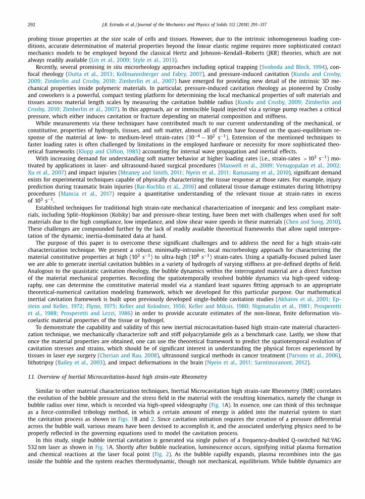
For the finite-deformation Kelvin–Voigt model, the dimensionless stress integral is given by
S ∗ = −1
2 Ca
[
5 −(
R ∗0 R ∗
)4
− 4 R ∗0 R ∗
]
−4 ̇ R ∗
Re R ∗, (50)
and for the SNS model, the ODE for the stress integral is given non-dimensionally by
De ̇ S ∗ + S ∗ = −1
2 Ca
[
5 −(
R ∗0 R ∗
)4
− 4 R ∗0 R ∗
]
−4 ̇ R ∗
Re R ∗−
4 De
3 Ca
˙ R ∗
R ∗R ∗3
R ∗3 − R ∗3 0
[
3
14 +
R ∗0 R ∗
−3
2
(
R ∗0 R ∗
)4
+ 2
7
(
R ∗0 R ∗
)7 ]
. (51)
Next, since the PDEs for the vapor mass fraction k ( r, t ) and the temperature T ( r, t ) inside the bubble, (15) and (22) , are
defined on the spatial domain 0 ≤ r ≤R ( t ), which possesses a moving boundary R ( t ), it is more convenient to express these
PDEs in terms of the dimensionless radial coordinate y = r/R (t) on the fixed domain 0 ≤ y ≤1. Further, to more conveniently
account for the temperature-dependence of the thermal conductivity K ( T ) in the non-dimensional governing equations, fol-
lowing Prosperetti et al. (1988) , we introduce the new dimensionless field variable,
θ = 1
K(T ∞ )
∫ T/T ∞
1 K(T ∞ ̂
θ ) d ̂ θ . (52)
Then the dimensionless PDEs governing the vapor mass fraction field k ( y, t ) and the field θ ( y, t ) inside the bubble (0 ≤ y ≤1)
are ⎧
⎪ ⎪ ⎪ ⎨
⎪ ⎪ ⎪ ⎩
∂k
∂t ∗+
v ∗m − ˙ R ∗y
R ∗∂k
∂y =
Fo
R ∗2 1
ρm y 2 ∂
∂y
(
ρm y 2 ∂k
∂y
)
,
κ
κ − 1
p ∗b
K ∗T ∗
(
∂θ
∂t ∗+
v ∗m − ˙ R ∗y
R ∗∂θ
∂y
)
= ˙ p ∗b +
χ
R ∗2 1
y 2 ∂
∂y
(
y 2 ∂θ
∂y
)
+ κ
κ − 1
p ∗b
K ∗T ∗Fo
R ∗2 C p , v −C p , g
C p
∂k
∂y
∂θ
∂y ,
(53)
with the dimensionless mixture velocity field inside the bubble v ∗m (y, t) given by
v ∗m =
1
κ p ∗b
[
(κ − 1) χ
R ∗∂θ
∂y −
1
3 R ∗y ˙ p ∗b
]
+ Fo
R ∗C p , v −C p , g
C p
∂k
∂y . (54)
Finally, the ODE governing the evolution of the dimensionless bubble pressure p ∗b (t) is
˙ p ∗b = 3
R ∗
[
−κ p ∗b ˙ R ∗ + (κ − 1)
χ
R ∗∂θ
∂y
∣∣∣∣y =1
+ κ p ∗b C p , v
C p (k (1))
Fo
1 − k (1)
1
R ∗∂k
∂y
∣∣∣∣y =1
]
. (55)
2.4.3. Boundary conditions for the PDEs
The PDEs (53) are accompanied by boundary conditions for k ( y, t ) and θ ( y, t ) at the bubble center (y = 0) and at the
bubble wall (y = 1) . First, at the origin, we have that ∂ k/∂ y | y =0 = ∂ θ/∂ y | y =0 = 0 . At the wall, using (52) , the temperature
boundary condition T (R ) = T ∞ becomes θ (1) = 0 . Finally, using (27) in conjunction with (20) and rearranging yields the
wall boundary condition for the vapor mass fraction:
k (1) =
[
1 + C p , v
C p , g
(p ∗b
p ∗v , sat − 1
)]−1
. (56)

302 J.B. Estrada et al. / Journal of the Mechanics and Physics of Solids 112 (2018) 291–317
Table 2
Material parameters.
Property Value Property Value
ρ 1060 kg/m 3 c 1430 m/s
p ∞ 101.3 kPa γ 5 . 6 × 10 −2 N/m
D 24 . 2 × 10 −6 m 2 /s κ 1.4
C p, v 1.62 kJ/kg ·K C p, g 1.00 kJ/kg ·K A 5 . 3 × 10 −5 W/m ·K 2 B 1 . 17 × 10 −2 W/m ·K p ref 1.17 ×10 8 kPa T ref 5200 K
T ∞ 298.15 K
2.5. Numerical method and model parameters
We obtain solutions to the coupled, non-dimensional ODEs (49) and (55) and PDEs (53) numerically. Following
Barajas and Johnsen (2017) , a fifth-order explicit Dormand–Prince Runge–Kutta method ( Prince and Dormand, 1981 ) with
adaptive step-size control is used to evolve the governing equations forward in time. Regarding spatial discretization of the
PDEs (55) , at each time substep, the PDEs are discretized on a mesh of N + 1 equidistant points in y -space ( Prosperetti et al.,
1988 ) inside the bubble and solved using second-order central differences. In the present work, we use N = 500 . Quantita-
tive values of the material parameters for the surrounding medium and the bubble contents used in this study are shown
in Table 2 and discussed further in Barajas and Johnsen (2017) .
2.6. Determining viscoelastic material parameters
To illustrate the practical workflow of the IMR technique, we characterize the non-linear, high strain-rate material
response of two polyacrylamide gel specimens of different stiffnesses. The extensive quasi-static characterization litera-
ture for polyacrylamide gels makes them ideal benchmarking soft matter materials for our IMR methodology. Since per-
forming calculations using the theoretical cavitation framework requires choosing a particular material constitutive model
( Gaudron et al., 2015 ), we have designed a user-adjustable workflow in which the iteration procedure begins with a sim-
ple fluid-like material model (i.e., a Newtonian fluid) followed by several material models of increasing complexity, i.e.,
the finite-deformation Kelvin–Voigt model and the SNS model. To begin the IMR procedure (see Fig. 3 ), the experimental
bubble-wall radius during the process of collapse and subsequent oscillation, R ( t ), is determined via straightforward image
processing of the experimental high-speed-image time-lapse series. From the experimental R ( t ) curve, two important input
parameters are extracted: the maximum radius R max at time t = t 0 , and the equilibrium radius R 0 for t → ∞ . 4 Since the
experimental radius data is discrete, in order to ensure R (t = t 0 ) = R max , the value for R max and the corresponding time t 0 are found by fitting a fourth-order polynomial to R ( t ) near the maximum bubble radius. In subsequent numerical calcula-
tions, the time t 0 identifies the initial state and corresponds to t = 0 in simulation time, and the initial conditions for the
Keller–Miksis equation are taken to be R (t = 0) = R max and ˙ R (t = 0) = 0 . The value of the equilibrium bubble radius R 0 is
estimated as the median of R ( t �0) after oscillations have ceased.
Regarding the initial conditions for the bubble contents, we take the initial temperature and the vapor pressure fields
inside the bubble to be spatially constant and given by T (r, t = 0) = T ∞ and p v (r, t = 0) = p v , sat (T ∞ ) , respectively. Then, to
determine the initial bubble pressure, p b (t = 0) = p v , sat (T ∞ ) + p g (t = 0) , it remains to determine the initial pressure of the
non-condensible gas, p g (t = 0) . To do so, we note that since the gas is unable to diffuse into the surrounding material, the
total mass of non-condensible gas inside the bubble remains constant in time, and since the gas temperature is T ∞ at both
t = 0 and as t → ∞ , using (18) 2 , we have that p g (t = 0) /p g (t → ∞ ) = (R 0 /R max ) 3 . At long times as t → ∞ , the surroundings
are stress-free, and mechanical equilibrium applied to the bubble requires that
p v , sat (T ∞ ) + p g (t = 0)
(R max
R 0
)3
︸ ︷︷ ︸
p g (t→∞ )
= p ∞ + 2 γ
R 0 . (57)
The initial pressure of the non-condensible gas may be deduced from (57) , and hence the initial bubble pressure is
p b (t = 0) = p v , sat (T ∞ ) +
(
p ∞ + 2 γ
R 0 − p v , sat (T ∞ )
)(R 0 R max
)3
, (58)
so that the initial bubble pressure, p b (t = 0) , is given through the experimentally-measured radius ratio R 0 /R max . Regarding
the initial conditions for the dimensionless PDEs (53) , for the vapor mass fraction field, consistent with the assumption
that the vapor pressure is constant and given through the saturation vapor pressure, we take k (y, t = 0) to be spatially
4 In general, R 0 represents the bubble radius corresponding to stress-free surroundings. In the case of laser-induced cavitation, we assume that the
surroundings are stress-free at long times so that R 0 = lim t→∞ R (t) . Of course, it is possible for R 0 and lim t → ∞ R ( t ) to not conincide and hence for a
residual stress field to exist in the surroundings as t → ∞ , but for simplicity, these effects are neglected in the present work.

J.B. Estrada et al. / Journal of the Mechanics and Physics of Solids 112 (2018) 291–317 303
µ
G
µ
G
G1
Neo-Hookean Elastic
Newtonian Fluid
Neo-Hookean Kelvin-Voigt
No
Yes
Behaviorcaptured by elastic fit?
No
Yes
Behaviorcaptured by
K-V fit?
No
Yes
Is the material a
fluid?
Vary G to fit collapsetime and oscillation
Radius measurementsfrom high-speed video
R(t), R0
Rmax/R0
determinesinitial pressure p
b(t =0)
Vary µ to fit rebound amplitudes
Vary G1 to fit rebound
amplitudes
LSQ fit entire curve for viscosity µ
LSQ fit entire curve for elastic modulus G
Relax constraint on G,LSQ fit over µ, G
Standard Non-Linear Solid
Relax constraint on G,LSQ fit over µ, G, G
1
G
µ
Fig. 3. Flowchart for the IMR material characterization technique. Experimental input consists of radius data acquired from high-speed video. Bubble
equilibrium radius R 0 and maximum expansion radius R max determine the initial gas pressure in the bubble to start the simulation. Material parameters
are then chosen to match the oscillation behavior.
constant and given by the value appearing in the wall boundary condition (56) , so that the vapor mass fraction initial
condition utilizes the initial bubble pressure (58) . For the dimensionless temperature field, the initial condition T (y, t = 0) =
T ∞ implies that θ (y, t = 0) = 0 .
The other free fitting parameters involved in the numerical simulations are the parameters describing the finite-
deformation viscoelastic response of the surrounding material, e.g., the equilibrium shear modulus G and the viscosity μ
for the finite-deformation Kelvin–Voigt model. Note that setting either G or μ to zero gives the respective results for the
purely viscous and purely elastic cases. The systematic procedure for determining these parameters is summarized in Fig. 3 .
First, a standard least squares fitting routine of the simulation results to the first three experimentally-measured peaks is
employed to yield estimates for material properties of the purely viscous and purely elastic one-parameter models. Then,
if the fits do not satisfactorily capture amplitude decay or oscillation frequency, the finite-deformation Kelvin–Voigt model
may be used to fit the experimental R ( t ) data by performing a two-parameter least squares fit over both G and μ. By em-
ploying standard convergence criteria (e.g., L 2 -norm), the number of constitutive parameters may be increased as necessary
by using a more complex material model such as the SNS model to provide the most robust fit. As a final remark, it is
important to note that while the particular material models discussed in the present work provide a good estimate for
many homogeneous and isotropic materials, the overall approach is general enough to allow inclusion of any user-specific
constitutive model to account for spherically-symmetric anisotropy or material inhomogeneities.
3. Materials and methods
3.1. Polyacrylamide preparation
Base 25 mm glass coverslips were hydrophilically functionalized using previously-developed protocols ( López-
Fagundo et al., 2014 ). Two cylindrical polyacrylamide hydrogel specimens were polymerized in custom Delrin molds with

304 J.B. Estrada et al. / Journal of the Mechanics and Physics of Solids 112 (2018) 291–317
0
200
400
600
800
Eng
inee
ring
Str
ess
[Pa]
0.1 0.2 0.30
1 – (Stretch Ratio, λ)
G∞
= 0.466 kPa, λ = 5×10⁻⁴ s-1⋅
G∞
= 0.456 kPa, λ = 5×10⁻³ s-1⋅
= 2.93 kPa, λ = 3×10⁻⁴ s-1⋅
G∞
= 3.00 kPa, λ = 3×10⁻³ s-1⋅
G∞
Fig. 4. Quasistatic compression characterization curves for polyacrylamide samples. Two stretch rates were tested for each gel. Experiments were fit to
Neo–Hookean free energy potentials, yielding quasistatic shear moduli of G ∞ , stiff = 2 . 97 ± 0 . 06 kPa and G ∞ , soft = 0 . 461 ± 0 . 004 kPa, for the stiff and soft
gels, respectively.
initial 15 mm diameter and 3 mm height at concentrations 5/0.03% and 10/0.06% acrylamide/bisacrylamide, respectively, for
45 min. Polyacrylamide gels were submerged completely in deionized water for 24 h before inducing cavitation and uniaxial
compression testing. Final dimensions of each gel post-swelling were about 16 mm in diameter and 8 mm in height.
3.2. Quasistatic characterization of polyacrylamide gels
After polyacrylamide gels were allowed to swell for 24 h, they were characterized mechanically in a custom unconfined
unaxial compression device consisting of a centrally-positioned linear actuator (Series A, Ultramotion, Cutchogue, NY) at-
tached to a force transducer (LCFA-25, Omega Engineering, Stamford, CT). A spherical tip attached to the transducer was
brought into contact with a 15 mm glass coverslip placed on top surface of the gel to ensure uniform uniaxial compres-
sion. Strain-rates were chosen to be between 10 −2 –10 −4 s −1 . Consistent with previous studies, tested gels exhibited Neo–
Hookean material behavior ( López-Fagundo et al., 2014 ) with quasistatic shear moduli ( G ∞ ) values of 2.97 ±0.06 kPa and
0.461 ±0.004 kPa for the stiff and soft gels, respectively ( Fig. 4 ).
3.3. Bubble generation and imaging
Single microcavitation bubbles were generated via one pulse of a user-adjustable 1–50 mJ, frequency-doubled Q-switched
532 nm Nd:YAG laser (Continuum, San Jose, CA), shown schematically in Fig. 1 A. Laser pulse energies were kept approxi-
mately equal over all tests. Pulses were aligned into the back port of a Nikon Ti-Eclipse inverted microscope (Nikon Instru-
ments, Tokyo, Japan) and reflected into the imaging objective using a 532 nm notch dichroic mirror (Semrock, Rochester, NY),
and were expanded to fill the back aperture of the imaging objective using a variable beam expander (Thorlabs, Newton,
NJ). Upon passing through the objective, pulses converged at the image plane as validated by continuous exposure align-
ment of a 635 nm laser diode (LDM635; Thorlabs, Newton, NJ). Microcavitation events were recorded with a Phantom v2511
high-speed CMOS camera (Vision Research, Wayne, NJ) using bright-field illumination with a halogen lamp. Samples were
imaged in 25mm cylindrical Chamlide magnetic chambers (Live Cell Instrument, Seoul, South Korea). For all tests, a 10 × /0.3
NA Plan Fluor objective (Nikon Instruments) was used to both focus and image the microcavitation events. Camera settings
were chosen to give maximum combined spatial (512 × 128 px) and temporal resolution (270,0 0 0 fps) in all tests. Exposure
time was set to 2 μs, and each video was chosen to be 101 total frames, with the first frame in each video designated as
a reference frame before arrival of the laser pulse. Cavitation events were initiated at a z-height of 1 mm above the top
surface of the bottom glass coverslip and x-y positions of at least 5 R max away from any previously-used location or edge
of the gel to sufficiently avoid boundary effects. Twenty cavitation tests per specimen were performed on each stiffness
polyacrylamide gel and a water control.

J.B. Estrada et al. / Journal of the Mechanics and Physics of Solids 112 (2018) 291–317 305
Calculating Bubble Radius
from High-Speed Brightfield Images
512 × 128 pixels at 270,000 fps
2.76 × 2.76 µm/px, 3.7 µs/frame
Acquire brightfield images during cavitation
Adjust for background intensity usingreference image to get differential image
Threshold image to get bubble edges
Sample points around convex hull andfit using Taubin (IEEE Trans, 1991)
Bubble Image, I
Differential Image, I – I0
Thresholded Image
Taubin radius fit
100 µm
Fig. 5. Image processing procedure for calculating bubble radius from high-speed brightfield images.
Polyacrylamide, G∞ = 2.97 kPa, n = 20
Polyacrylamide, G∞ = 0.461 kPa, n = 20
Water, n = 20
0 2 60
0.5
1
Nor
mal
ized
Rad
ius
R*
= R
( t)
Rm
ax
4
Normalized Time t* = t
Rmax
√p
∞
ρ
Fig. 6. Normalized bubble radius vs. time for water and both tested stiffnesses of polyacrylamide. For all material platforms, dynamics coalesced into
distinct bands.
306 J.B. Estrada et al. / Journal of the Mechanics and Physics of Solids 112 (2018) 291–317
Leas
t Squ
ares
Err
or
10-5 10-4 10-3 10-2 10-1
×10-4
Viscosity, µ [Pa s]
0
3
4
5
6
7
1
2
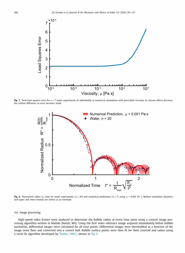
Fig. 7. Total least squares error for n = 7 water experiments fit individually to numerical simulations with prescribed viscosity. As viscous effects decrease,
the relative difference in error becomes small.
0 1 20
0.5
1
Nor
mal
ized
Rad
ius
R*
= R
( t)
Rm
ax
Normalized Time t* = t
Rmax
√p
∞
ρ
Numerical Prediction, µ = 0.001 Pa s Water, n = 20
Fig. 8. Normalized radius vs. time for water experiments ( n = 20 ) and numerical predictions ( n = 7 ) using µ = 0 . 001 Pa · s. Median simulation dynamics
and upper and lower bounds are shown as an envelope.
3.4. Image processing
High-speed video frames were analyzed to determine the bubble radius at every time point using a custom image pro-
cessing algorithm written in Matlab (Natick, MA). Using the first video reference image acquired immediately before bubble
nucleation, differential images were calculated for all time points. Differential images were thresholded as a function of the
image noise floor and converted into a convex hull. Bubble surface points were then fit for their centroid and radius using
a circle fit algorithm developed by Taubin (1991) , shown in Fig 5 .

J.B. Estrada et al. / Journal of the Mechanics and Physics of Solids 112 (2018) 291–317 307
B
A
Bub
ble
Rad
ius,
R [µ
m]
0
50
100
150
200
250
300
350
µMaterial Model
10-4 10-0.5[Pa s]
NewtonianFluid
Time, t [µs]0 10050 200150
GMaterial Model
Neo-HookeanElastic
101 105[Pa]
Time, t [µs]0 10050 200150
Bub
ble
Rad
ius,
R [µ
m]
0
50
100
150
200
250
300
350
Fig. 9. Roles of shear modulus and dynamic viscosity in the numerical fit. For both plots, experimental data from a representative stiff polyacrylamide
inertial cavitation event (orange squares) are overlaid on a one-parameter sweep using (A) a Newtonian Fluid model and (B) a Neo–Hookean elastic model.
With increasing viscosity, resulting rebound amplitudes are suppressed, while initial collapse time is relatively unchanged. With increasing shear modulus,
resulting rebound frequency increases and initial collapse time correspondingly decreases. Dashed-dotted line represents the inviscid, zero-elastic fluid
case. For both plots, top and bottom horizontal dashed black lines denote R max and R 0 . (For interpretation of the references to color in this figure legend,
the reader is referred to the web version of this article.)
3.5. Experimental precision assessment
The maximum bubble radius for each tested polyacrylamide gel varied moderately, with R max = 388 ± 35 μm and R max =
430 ± 17 μm for the stiffer and softer gels, respectively. Non-dimensionalization of the bubble dynamics highlights material-
specific similarities for both stiffnesses of polyacrylamide and water as shown in Fig. 6 .
3.6. Least squares error and mean values
Least squares error (LSE) is defined discretely by minimizing the perpendicular offset between experimental data points
and the numerical simulation. Minimizing the discrete least squares error in the first three peaks gives the best estimate
of the viscoelastic properties of the gel. To determine mean viscoelastic material properties (denoted as x ) and standard
deviation σ̄ , fits performed to the first collapse over n = 20 experiments were weighted by the goodness of least squares fit
308 J.B. Estrada et al. / Journal of the Mechanics and Physics of Solids 112 (2018) 291–317
Material Model
Neo-HookeanKelvin-Voigt
µ
G
G
101
105
[Pa]
µ10-4 10-0.5[Pa s]
Neo-Hookean ElasticNewtonian FluidN-H Kelvin-Voigt
Time, t [µs]
µs
0 10050 200150
Bub
ble
Rad
ius,
R [µ
m]
0
50tc≈30
100
150
200
250
300
350
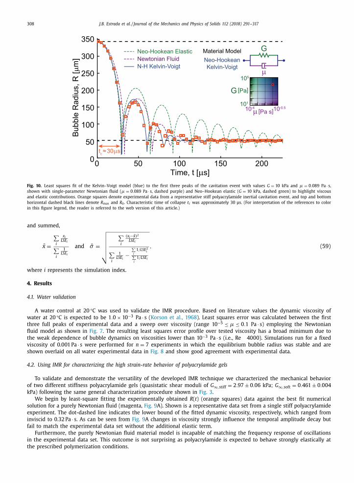
Fig. 10. Least squares fit of the Kelvin–Voigt model (blue) to the first three peaks of the cavitation event with values G = 10 kPa and µ = 0 . 089 Pa · s, shown with single-parameter Newtonian fluid ( µ = 0 . 089 Pa · s, dashed purple) and Neo–Hookean elastic ( G = 10 kPa, dashed green) to highlight viscous
and elastic contributions. Orange squares denote experimental data from a representative stiff polyacrylamide inertial cavitation event, and top and bottom
horizontal dashed black lines denote R max and R 0 . Characteristic time of collapse t c was approximately 30 μs. (For interpretation of the references to color
in this figure legend, the reader is referred to the web version of this article.)
and summed,
x̄ =
∑
i
x i LSE i
∑
i
1 LSE i
and σ̄ =
√ √ √ √ √ √
∑
i
(x i −x̄ ) 2
LSE i
∑
i
1 LSE i
−∑
i 1 /LSE 2
i ∑
i 1 /LSE i
, (59)
where i represents the simulation index.
4. Results
4.1. Water validation
A water control at 20 °C was used to validate the IMR procedure. Based on literature values the dynamic viscosity of
water at 20 °C is expected to be 1 . 0 × 10 −3 Pa · s ( Korson et al., 1968 ). Least squares error was calculated between the first
three full peaks of experimental data and a sweep over viscosity (range 10 −5 ≤ µ ≤ 0 . 1 Pa · s) employing the Newtonian
fluid model as shown in Fig. 7 . The resulting least squares error profile over tested viscosity has a broad minimum due to
the weak dependence of bubble dynamics on viscosities lower than 10 −3 Pa · s (i.e., Re � 40 0 0). Simulations run for a fixed
viscosity of 0.001 Pa · s were performed for n = 7 experiments in which the equilibrium bubble radius was stable and are
shown overlaid on all water experimental data in Fig. 8 and show good agreement with experimental data.
4.2. Using IMR for characterizing the high strain-rate behavior of polyacrylamide gels
To validate and demonstrate the versatility of the developed IMR technique we characterized the mechanical behavior
of two different stiffness polyacrylamide gels (quasistatic shear moduli of G ∞ , stiff = 2 . 97 ± 0 . 06 kPa; G ∞ , soft = 0 . 461 ± 0 . 004
kPa) following the same general characterization procedure shown in Fig. 3 .
We begin by least-square fitting the experimentally obtained R ( t ) (orange squares) data against the best fit numerical
solution for a purely Newtonian fluid (magenta, Fig. 9 A). Shown is a representative data set from a single stiff polyacrylamide
experiment. The dot-dashed line indicates the lower bound of the fitted dynamic viscosity, respectively, which ranged from
inviscid to 0.32 Pa · s. As can be seen from Fig. 9 A changes in viscosity strongly influence the temporal amplitude decay but
fail to match the experimental data set without the additional elastic term.
Furthermore, the purely Newtonian fluid material model is incapable of matching the frequency response of oscillations
in the experimental data set. This outcome is not surprising as polyacrylamide is expected to behave strongly elastically at
the prescribed polymerization conditions.
J.B. Estrada et al. / Journal of the Mechanics and Physics of Solids 112 (2018) 291–317 309
A
B
Bub
ble
Rad
ius,
R [µ
m]
50
100
0
150
200
250
300
350
Time, t [µs]0 10050 200150
Material Model
StandardNon-Linear
Solid104 108
G1 [Pa]
µ
G
G1
Leas
t Squ
ares
Err
or
×10-5
104 105 106 107 108
Elastic Constant, G1 [Pa]
0
2
4
6
8
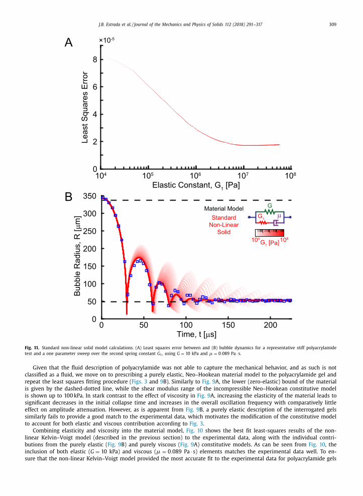
Fig. 11. Standard non-linear solid model calculations. (A) Least squares error between and (B) bubble dynamics for a representative stiff polyacrylamide
test and a one parameter sweep over the second spring constant G 1 , using G = 10 kPa and µ = 0 . 089 Pa · s.
Given that the fluid description of polyacrylamide was not able to capture the mechanical behavior, and as such is not
classified as a fluid, we move on to prescribing a purely elastic, Neo–Hookean material model to the polyacrylamide gel and
repeat the least squares fitting procedure ( Figs. 3 and 9 B). Similarly to Fig. 9 A, the lower (zero-elastic) bound of the material
is given by the dashed-dotted line, while the shear modulus range of the incompressible Neo–Hookean constitutive model
is shown up to 100 kPa. In stark contrast to the effect of viscosity in Fig. 9 A, increasing the elasticity of the material leads to
significant decreases in the initial collapse time and increases in the overall oscillation frequency with comparatively little
effect on amplitude attenuation. However, as is apparent from Fig. 9 B, a purely elastic description of the interrogated gels
similarly fails to provide a good match to the experimental data, which motivates the modification of the constitutive model
to account for both elastic and viscous contribution according to Fig. 3 .
Combining elasticity and viscosity into the material model, Fig. 10 shows the best fit least-squares results of the non-
linear Kelvin–Voigt model (described in the previous section) to the experimental data, along with the individual contri-
butions from the purely elastic ( Fig. 9 B) and purely viscous ( Fig. 9 A) constitutive models. As can be seen from Fig. 10 , the
inclusion of both elastic ( G = 10 kPa) and viscous ( µ = 0 . 089 Pa · s) elements matches the experimental data well. To en-
sure that the non-linear Kelvin–Voigt model provided the most accurate fit to the experimental data for polyacrylamide gels

310 J.B. Estrada et al. / Journal of the Mechanics and Physics of Solids 112 (2018) 291–317
µ1
µ1
G∞
quasistatic
Lump springs
t1=
G1
G=G∞+G
1+...+G
n
Lump dashpotsµ=µ
n+1+...+µ
N–1+µ
N
µ2
G2
µ3
G3
µn
Gn
µn+1
Gn+1
µN–1
GN–1
µN
GN
G1
General material behavior with a spectrum of relaxation times
> t2
frozen timescales during cavitaiton
dashpots flowduring cavitation
> >> >> >t3
tn t
c
tn+1
tN–1
tN
G µ
Lumped Kelvin-Voigt modelfor cavitation process of
characteristic time tc
Fig. 12. General material behavior with a spectrum of relaxation times. A viscoelastic material modeled by a spectrum of N Maxwell branches with
different relaxation times can be lumped into elastic and viscous parts when probed at a certain frequency, or characteristic time t c . While branches of
long relaxation time do not have time to relax during cavitation and appear frozen, branches of short relaxation time flow easily. The lumped Kelvin–
Voigt model shear modulus G and viscosity μ are then combinations of the springs and dashpots for branches with longer and shorter relaxation times,
respectively.
tested, we also characterized the same gels using a standard non-linear solid ( Fig. 3 ), which failed to produce any significant
increase in accuracy beyond the simpler Kelvin–Voigt model.
To produce the final estimate for the Kelvin–Voigt material parameters, the shear modulus and material viscosities were
averaged over n = 20 experiments for each of the two different polyacrylamide concentrations. However, in order to better
account for variability between experiments, the total estimate on G and μ were appropriately weighted by the goodness
of their least squares fit using (59) , producing the shear moduli of G stiff = 7 . 69 ± 1 . 12 kPa and G soft = 2 . 12 ± 0 . 70 kPa and
viscosities of µstiff = 0 . 101 ± 0 . 023 Pa · s and µsoft = 0 . 118 ± 0 . 014 Pa · s, for the two gels, respectively.
While the material model for polyacrylamide was chosen to be Neo–Hookean Kelvin–Voigt as per the flowchart shown
in Fig. 3 , the standard non-linear solid model was also explored as a potential option for polyacrylamide. The resulting least
squares error profile suggests a high value for G 1 as the optimal fit, as shown in Fig. 11 . Notably, in the limit of G 1 → ∞ ,
or more precisely, as the Maxwell branch relaxation time μ/ G 1 becomes much smaller than the characteristic collapse time
t c , the standard non-linear solid model converges to the Neo–Hookean Kelvin–Voigt model, suggesting validity of our model
choice.
The inclusion of another spring constant G 1 has important effects on the resulting bubble dynamics. When values of
G 1 are on the order of G (i.e. when μ/ G 1 approaches the characteristic collapse time), oscillation amplitudes are increased.
Additionally, the relative ratios between subsequent peak amplitudes (e.g. R (1) max /R
(2) max , R
(2) max /R
(3) max ) increase as G 1 → G . As our
numerical fits even for the two-parameter Neo–Hookean Kelvin–Voigt model under-predicted later peaks, we found that the
increasing influence of an added spring increased least squares error for the tested polyacrylamide gels as shown in Fig. 11 A.
Lowest least squares error was found as G 1 → ∞ as shown in Fig. 11 B, which confirmed our choice of the two-parameter
model.
5. Discussion
The presented IMR technique is a robust, minimally-intrusive, local microrheology approach for characterizing the ma-
terial constitutive properties at high (10 3 s −1 ) to ultra-high (10 8 s −1 ) strain-rates. By combining simple, high-speed videog-
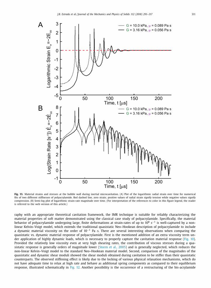
J.B. Estrada et al. / Journal of the Mechanics and Physics of Solids 112 (2018) 291–317 311
A
B
0 10050 200150
G = 10.0 kPa, µ = 0.089 Pa sG = 3.16 kPa, µ = 0.056 Pa s
Time, t [µs]
Log(
Str
ain
Rat
e [s
-1])
Err=
−2E
θθ
••
-1
0
1
2
3
4
5
7
6
8
G = 10.0 kPa, µ = 0.089 Pa sG = 3.16 kPa, µ = 0.056 Pa s
Time, t [µs]0 10050 200150
Loga
rithm
ic S
trai
n E
rr=
−2E
θθ
-5
-2
-4
-3
-1
0
1
2
3
Fig. 13. Material strains and stresses at the bubble wall during inertial microcavitation. (A) Plot of the logarithmic radial strain over time for numerical
fits of two different stiffnesses of polyacrylamide. Red dashed line, zero strain; positive values of radial strain signify tension while negative values signify
compression. (B) Semi-log plot of logarithmic strain-rate magnitude over time. (For interpretation of the references to color in this figure legend, the reader
is referred to the web version of this article.)
raphy with an appropriate theoretical cavitation framework, the IMR technique is suitable for reliably characterizing the
material properties of soft matter demonstrated using the classical case study of polyacrylamide. Specifically, the material
behavior of polyacrylamide undergoing large, finite deformations at strain-rates of up to 10 8 s −1 is well-captured by a non-
linear Kelvin–Voigt model, which extends the traditional quasistatic Neo–Hookean description of polyacrylamide to include
a dynamic material viscosity on the order of 10 −1 Pa · s. There are several interesting observations when comparing the
quasistatic vs. dynamic material response of polyacrylamide. First is the mentioned addition of an extra viscosity term un-
der application of highly dynamic loads, which is necessary to properly capture the cavitation material response ( Fig. 10 ).
Provided the relatively low viscosity even at very high shearing rates, the contribution of viscous stresses during a qua-
sistatic response is generally orders of magnitude lower ( Storm et al., 2005 ) and is generally neglected, which reduces the
non-linear Kelvin–Voigt model to the standard Neo–Hookean material model. Second, comparison of the magnitudes of the
quasistatic and dynamic shear moduli showed the shear moduli obtained during cavitation to be stiffer than their quasistatic
counterparts. The observed stiffening effect is likely due to the locking of various physical relaxation mechanisms, which do
not have adequate time to relax at high rate and behave as additional spring components as compared to their equilibrium
response, illustrated schematically in Fig. 12 . Another possibility is the occurrence of a restructuring of the bis-acrylamide

312 J.B. Estrada et al. / Journal of the Mechanics and Physics of Solids 112 (2018) 291–317
G = 10.0 kPa, µ = 0.089 Pa sG = 3.16 kPa, µ = 0.056 Pa s
Compressive StressTensile Stress
0 10050 200150Time, t [µs]
Log |
Dev
iato
ric S
tres
s s rr
=−
2sθ
θ [P
a]|
-1
1
0
2
3
4
5
6
8
7
Fig. 14. Semi-log plot of deviatoric Cauchy stress magnitude at the bubble wall over time. Linear decrease of peak magnitudes suggests an exponential
decay envelope. Red portions of each curve signify tensile radial stress, while blue portions signify compressive stress. (For interpretation of the references
to color in this figure legend, the reader is referred to the web version of this article.)
cross-linked structure due to the large expansion and contraction strains. However, detailed analysis of the physical origin
of the observed stiffening behavior of the material is beyond the scope of this work.
Interestingly, the relative ratio between the gel stiffnesses was significantly lower at ultra-high strain-rates, with
G stiff /G soft = 3 . 62 and G ∞ , stiff /G ∞ , soft = 6 . 46 , suggesting that the stiffness scaling of the incorporation levels between bis and
acrylamide monomer as was established under quasistatic loading is not extendable into the fast dynamic loading regime.
Thus, use of quasistatic tests cannot be assumed to adequately replace testing for ultra-high strain-rate material response.
5.1. Material stresses and strains due to cavitation
Once the characterization of the material properties is achieved, the solution to Eqs. (49) –( 55) can be utilized to closely
examine the stress and strain evolution of the material during collapse, subsequent rebounds, and oscillation as both a func-
tion of time and position. Such an analysis allows one to build an understanding of the associated strains, strain-rates and
stresses with cavitation in soft matter. While there are many state variables that can be plotted against space and time,
we purposefully focus on the most relevant quantities to describe the stress-strain field in the surrounding material. Shown
in Fig. 13 are the strains, strain-rates, and stresses at the bubble wall as a function of time for representative numerical
bubble dynamics solutions obtained by least squares fitting one test of each of the two different concentrations of polyacry-
lamide gels. Radial Hencky strain, E rr = −2 ln (r/r 0 ) , evaluated at the bubble wall ( Fig. 13 A) is finite ( �0.05) over the first
∼5 oscillations of the bubble, with large peak values in both initial radial compression and subsequent radial tension at
collapse.
The primary collapse event occurs extremely quickly ( ∼1 μs) producing peak strain-rates at the bubble wall on the
order of 10 7 –10 8 s −1 ( Fig. 13 B). Strain-rates also change rapidly as the bubble oscillates between the expansion and collapse
phases with an exponential decay as suggested by the linear decrease of peaks as a function of time on the semi-log plot
( Fig. 13 B). The radial stresses, shown in Fig. 14 , also decay exponentially with time but exhibit a behavior distinctly different
from the strains during the peak strain-rates of primary collapse. The presence of material viscosity breaks the temporal
symmetry in the stress response when compared to the symmetric Hencky strain profile.
In addition to temporal quantities at the bubble wall, field quantities in the material can be calculated at specific time-
points. For example, at peak radial compression and tension, we can examine strain and stress quantities as a function of
radial position. This type of information is often useful in developing scaling laws or damage criteria as a function of the
underlying material properties or microstructure ( Baker, 2015; Rosakis et al., 2015 ). Fig. 15 A shows a plot relating the refer-
ence configuration (equilibrium) radial coordinate to the deformed radial coordinate during the peak radial expansion (red)
and peak radial compression (blue). The dashed line signifies the no-deformation case where the deformed position equals
the equilibrium position, which when approached asymptotically, signifies the small strain, linear viscoelastic regime.
Given the strongly inhomogeneous loading nature of cavitation, it is useful to establish a convergence length, i.e., a non-
dimensional distance beyond which the solution to Eqs. (49) –( 55 ) can be linearized, to pave the way for developing simpler,
analytically-closed form solutions under the assumption that stresses and strains in the immediate vicinity of the bubble
do not need to be fully resolved. As an example, the positions where strains become small, i.e. E rr < 0.05 (see Fig. 15 B),
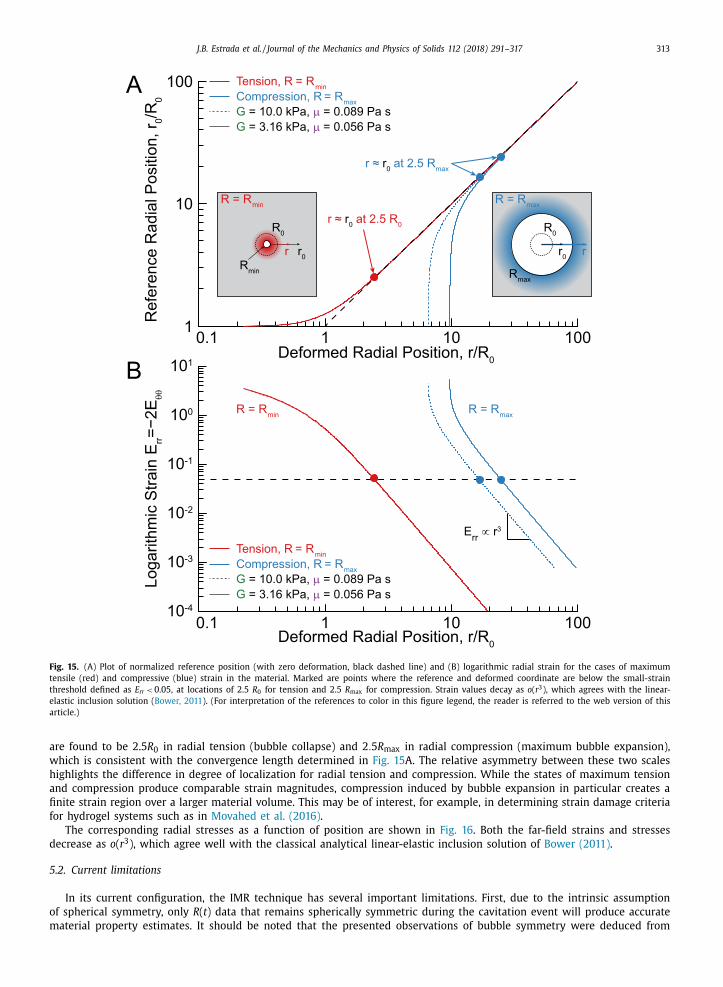
J.B. Estrada et al. / Journal of the Mechanics and Physics of Solids 112 (2018) 291–317 313
A
B
Ref
eren
ce R
adia
l Pos
ition
, r0/
R0
Deformed Radial Position, r/R0
110.1
10
10
100
100
r ≈ r0 at 2.5 R
max
G = 10.0 kPa, µ = 0.089 Pa sG = 3.16 kPa, µ = 0.056 Pa s
Compression, R = Rmax
Tension, R = Rmin
Rmax
R0
R = Rmax
r0
rR
min
R0
R = Rmin
r0
r
r ≈ r0 at 2.5 R
0
Loga
rithm
ic S
trai
n E
rr=
−2E
θθ
Deformed Radial Position, r/R0
10.1 10 10010-4
10-3
10-2
10-1
100
101
Err
∝ r3
G = 10.0 kPa, µ = 0.089 Pa sG = 3.16 kPa, µ = 0.056 Pa s
Compression, R = Rmax
Tension, R = Rmin
R = Rmax
R = Rmin
Fig. 15. (A) Plot of normalized reference position (with zero deformation, black dashed line) and (B) logarithmic radial strain for the cases of maximum
tensile (red) and compressive (blue) strain in the material. Marked are points where the reference and deformed coordinate are below the small-strain
threshold defined as E rr < 0.05, at locations of 2.5 R 0 for tension and 2.5 R max for compression. Strain values decay as o ( r 3 ), which agrees with the linear-
elastic inclusion solution ( Bower, 2011 ). (For interpretation of the references to color in this figure legend, the reader is referred to the web version of this
article.)
are found to be 2.5 R 0 in radial tension (bubble collapse) and 2 . 5 R max in radial compression (maximum bubble expansion),
which is consistent with the convergence length determined in Fig. 15 A. The relative asymmetry between these two scales
highlights the difference in degree of localization for radial tension and compression. While the states of maximum tension
and compression produce comparable strain magnitudes, compression induced by bubble expansion in particular creates a
finite strain region over a larger material volume. This may be of interest, for example, in determining strain damage criteria
for hydrogel systems such as in Movahed et al. (2016) .
The corresponding radial stresses as a function of position are shown in Fig. 16 . Both the far-field strains and stresses
decrease as o ( r 3 ), which agree well with the classical analytical linear-elastic inclusion solution of Bower (2011) .
5.2. Current limitations
In its current configuration, the IMR technique has several important limitations. First, due to the intrinsic assumption
of spherical symmetry, only R ( t ) data that remains spherically symmetric during the cavitation event will produce accurate
material property estimates. It should be noted that the presented observations of bubble symmetry were deduced from

314 J.B. Estrada et al. / Journal of the Mechanics and Physics of Solids 112 (2018) 291–317
|Dev
iato
ric S
tres
s s rr
=−
2sθ
θ [P
a]|
Deformed Radial Position, r/R0
10.1 10 100101
102
103
104
105
106
G = 10.0 kPa, µ = 0.089 Pa sG = 3.16 kPa, µ = 0.056 Pa s
Compression, R = Rmax
Tension, R = Rmin
srr
∝ r3
R = Rmin
R = Rmax
Fig. 16. Deviatoric Cauchy stress versus deformed position for the cases of maximum tensile (red) and compressive (blue) strain in the material. Marked
are points where the reference and deformed coordinate are below the small-strain threshold defined as E rr < 0.05, at locations of 2.5 R 0 for tension and
2 . 5 R max for compression. Strain and stress values decay as o ( r 3 ), which agrees with the linear-elastic inclusion solution ( Bower, 2011 ). (For interpretation of
the references to color in this figure legend, the reader is referred to the web version of this article.)
a single camera midplane (i.e., 2D cylindrical projection) observation, which previously was shown to be an appropriate
experimental estimate (e.g. Fig 2 of Akhatov et al. (2001) ). In homogeneous materials, spherical symmetry, for non-violent,
subsonic to sonic bubble collapses can typically be ensured by cavitating 2–3 maximum bubble diameters away from bound-
aries that feature significant impedance changes. In scenarios where the local bubble collapse speed is to be expected to
be of Mach numbers much greater than one, spherical symmetry may be lost near the collapse stage due to non-linear
amplification of slight perturbations in the pressure field in the form of material or geometric imperfections. Properly re-
constructing and analyzing non-symmetric three-dimensional cavitation dynamics remains challenging both from a high-
speed imaging and reconstruction standpoint as well as from a numerical perspective as the momentum and conservation
of mass equations must be solved in 3D, which is computationally challenging. Second, the current mathematical framework
assumes all of the to-be-employed material models to be incompressible in the near field, which is an adequate assumption
for most tissues and hydrogels but may not be appropriate for foams and other highly compressible materials. Inclusion of
compressible material models is possible; however, the literature is still in its infancy when it comes to non-linear, highly
compressible material descriptions. Third, while the current approach does not require independent measures of bubble
pressure or temperatures, mainly due to the fairly simple constitutive models employed, future investigations of more com-
plex materials might require the addition of independent measurements of pressure and/or temperature to ensure solution
uniqueness and to validate the modeling assumptions for the bubble contents. Fourth, the current theoretical treatment of
cavitation assumes ˙ R /c to be small, which may not be sufficiently accurate close to the bubble collapse phase, where shock
waves may be produced. For polyacrylamide, the highest values of ˙ R /c recorded in simulations were approximately 0.4 at
the collapse, however, for lower viscosity materials, ˙ R /c may approach or exceed 1. While inclusion of the higher order
terms in ˙ R /c is possible and well-documented in the literature ( Lezzi and Prosperetti, 1987 ), the current imaging system
does not have enough temporal resolution ( < 1 μs) to fully resolve such detail. Finally, since the bubble lifetime is directly
proportional to the maximum bubble radius, proper temporal resolution becomes increasingly challenging for bubble sizes
10 μm and below. We anticipate that many of these challenges will be overcome and addressed in future studies that will
build upon the experimental and theoretical framework established herein.
6. Conclusion
IMR represents a new approach for determining the viscoelastic material properties of soft matter at high (10 3 s −1 ) to
ultra-high (10 8 s −1 ) strain-rates via inertial cavitation that requires only a single pulsed laser and a high-speed imaging
platform, which can be easily integrated into commercially available inverted or upright light microscopes. By combining
high-speed video of bubble oscillation with an appropriate theoretical model of cavitation-bubble collapse, we demonstrate
the ability to discern mechanical properties and field variables at previously undocumented strain-rates in materials as
soft as a few kPa. Specifically, we show that the material behavior of polyacrylamide undergoing large, finite deformations
(| E rr | > 0.05) at strain-rates of up to 10 8 s −1 is well-captured by a non-linear Kelvin–Voigt model, which extends the
J.B. Estrada et al. / Journal of the Mechanics and Physics of Solids 112 (2018) 291–317 315
traditional quasistatic Neo–Hookean description of polyacrylamide to include a dynamic material viscosity on the order of
10 −1 Pa · s. Since cavitation induction is achieved via spot focusing of a single laser pulse, this technique is minimally invasive and
can characterize material properties in three dimensions at length scales of single microns to millimeters. As such this tech-
nique shows great promise for use of the interrogation of in vivo materials as well as for samples of small size, odd shape,
or high compliance, which may otherwise not be easily mountable in conventional dynamic testing apparatus. The suitabil-
ity of this inertial cavitation rheology technique is demonstrated and benchmarked using the well-characterized hydrogel
polyacrylamide and shows that, under high strain-rate loading, stress contributions due to viscosity effects need to be in-
cluded alongside the well-known Neo–Hookean elastic nature of polyacrylamide. Furthermore, this technique has excellent
precision and repeatability in its measurements, particularly when compared to other local soft matter tribology methods
including nano- and microindentation.
In sum, IMR may fill the void of a simple and robust microrheology technique to determine soft matter and tissue
properties at high to ultra-high strain-rates, as well as to provide a high-fidelity platform for understanding inhomogeneous
cavitation stresses and strains as arise in many natural, biological, and engineering applications.
Acknowledgments
CF gratefully acknowledges support from the Office of Naval Research (Dr. Timothy Bentley) under grants N0 0 0141612872
and N0 0 0141712058. EJ acknowledges support from NSF grant CBET 1253157. JBE acknowledges support from a Graduate
Assistance in Areas of National Need (GAANN) fellowship from the Brown University Institute for Molecular and Nanoscale
Innovation. This research was conducted using computational resources and services at the Center for Computation and
Visualization, Brown University.
Appendix A. Keller–Miksis Formulation
The first step in deriving the Keller–Miksis equation is to recast the momentum balance (3) in terms of the potential
function φ( r, t ) as
ρ
(
∂ 2 φ
∂ r∂ t +
∂φ
∂r
∂ 2 φ
∂r 2
)
= −∂ p
∂r +
∂s rr ∂r
+ 2
r ( s rr − s θθ ) (A.1)
and then integrate (A.1) over r from r = R to r → ∞ to obtain
ρ
[
−∂φ
∂t
∣∣∣∣r= R
−1
2
(
∂φ
∂r
∣∣∣∣r= R
)2 ]
= −( p ∞ − p(R ) ) − s rr (R ) +
∫ ∞
R
2
r ( s rr − s θθ ) dr. (A.2)
In (A.2) , we have applied the far-field stress boundary condition – namely, that the far-field stress state consists of a con-
stant isotropic pressure p ∞ , i.e., s rr (r → ∞ ) = 0 and p(r → ∞ ) = p ∞ . The bubble-wall boundary conditions consist of the
kinematic boundary condition v (R, t) = ∂ φ/∂ r| r= R = ˙ R (t) and the traction boundary condition, which relates the radial com-
ponent of the Cauchy stress at the bubble wall, s rr (R, t) − p(R, t) , to the gas pressure inside the bubble, p b ( t ), and the surface
tension, γ , through
p(R ) − s rr (R ) = p b −2 γ
R . (A.3)
Defining the time-dependent quantity S ( t ) through
S =
∫ ∞
R
2
r ( s rr − s θθ ) dr, (A.4)
using the wall boundary conditions in (A.2) , and rearranging yields
∂φ
∂t
∣∣∣∣r= R
= −1
2 ˙ R 2 −
1
ρ
(
p b −2 γ
R + S − p ∞
)
. (A.5)
Next, from (6)
⎧
⎪ ⎪ ⎪ ⎨
⎪ ⎪ ⎪ ⎩
∂φ
∂t
∣∣∣∣r= R
= 1
R f ′ (
t −R
c
)
∂φ
∂r
∣∣∣∣r= R
= ˙ R = −1
cR f ′ (
t −R
c
)
−1
R 2 f
(
t −R
c
)
,
(A.6)

316 J.B. Estrada et al. / Journal of the Mechanics and Physics of Solids 112 (2018) 291–317
where f ′ represents the derivative of the arbitrary function f . Combining Eq. (A.6) to eliminate f ′ leads to an alternate ex- pression for ∂ φ/∂ t| r= R :
∂φ
∂t
∣∣∣∣r= R
= −c
R 2 f
(
t −R
c
)
− c ˙ R . (A.7)
Using (A.6) 1 and (A.7) in conjunction with (A.5) , we have ⎧
⎪ ⎪ ⎨
⎪ ⎪ ⎩
1
R f ′ (
t −R
c
)
= −1
2 ˙ R 2 −
1
ρ
(
p b −2 γ
R + S − p ∞
)
,
−c
R 2 f
(
t −R
c
)
− c ˙ R = −1
2 ˙ R 2 −
1
ρ
(
p b −2 γ
R + S − p ∞
)
.
(A.8)
Taking the time derivative of (A.8) 2 and combining with (A.8) 1 to eliminate f ′ yields the Keller–Miksis equation:
(
1 −˙ R
c
)
R ̈R + 3
2
(
1 −˙ R
3 c
)
˙ R 2 = 1
ρ
(
1 + ˙ R
c
)(
p b −2 γ
R + S − p ∞
)
+ 1
ρ
R
c
˙ (
p b −2 γ
R + S
)
. (A.9)
Supplementary material
Supplementary material associated with this article can be found, in the online version, at 10.1016/j.jmps.2017.12.006 .
References
Akhatov, I. , Lindau, O. , Topolnikov, A. , Mettin, R. , Vakhitova, N. , Lauterborn, W. , 2001. Collapse and rebound of a laser-induced cavitation bubble. Phys. Fluids 13 (10), 2805–2819 .
Bailey, M. , Khokhlova, V. , Sapozhnikov, O. , Kargl, S. , Crum, L. , 2003. Physical mechanisms of the therapeutic effect of ultrasound (a review). Acoust. Phys. 49 (4), 437–464 .
Baker, B. , et al. , 2015. Cell-mediated fibre recruitment drives extracellular matrix mechanosensing in engineered fibrillar microenvironments. Nat. Mater. 14 (12), 1262–1268 .
Bar-Kochba, E. , Scimone, M. , Estrada, J. , Franck, C. , 2016. Strain and rate-dependent neuronal injury in a 3d in vitro compression model of traumatic brain injury. Sci. Rep. 6, 30550 .
Barajas, C. , Johnsen, E. , 2017. The effects of heat and mass diffusion on freely oscillating bubbles in a viscoelastic, tissue-like medium. J. Acoust. Soc. Am. 141 (2), 908–918 .
Bower, A. , 2011. Applied Mechanics of Solids. CRC Press, Boca Raton, Florida, USA . Chen, W. , Song, B. , 2010. Split Hopkinson (Kolsky) Bar: Design, Testing and Applications. Springer, New York, USA . Cherian, A. , Rau, K. , 2008. Pulsed-laser-induced damage in rat corneas: time-resolved imaging of physical effects and acute biological response. J. Biomed.
Opt. 13 (2), 024009 . Dutta, S. , Mbi, A. , Arevalo, R. , Blair, D. , 2013. Development of a confocal rheometer for soft and biological materials. Rev. Sci. Instrum. 84, 063702 . Ebenstein, D.M. , Pruitt, L.A. , 2004. Nanoindentation of soft hydrated materials for application to vascular tissues. J. Biomed. Mater. Res. A 69A (2), 222–232 . Epstein, D. , Keller, J. , 1972. Expansion and contraction of planar, cylindrical, and spherical underwater gas bubbles. J. Acoust. Soc. Am. 52 (3), 975–980 . Flynn, H. , 1975. Cavitation dynamics. i. A mathematical formulation. J. Acoust. Soc. Am. 57 (6), 1379–1396 . Fujikawa, S. , Akamatsu, T. , 1980. Effects of the non-equilibrium condensation of vapor on the pressure wave produced by the collapse of a bubble in a
liquid. J. Fluid Mech. 97 (3), 481–512 . Gaudron, R. , Warnez, M. , Johnsen, E. , 2015. Bubble dynamics in a viscoelastic medium with nonlinear elasticity. J. Fluid Mech. 766, 54–75 . Hu, Y. , You, J.-O. , Auguste, D. , Suo, Z. , Vlassak, J. , 2011. Indentation: a simple, nondestructive method for characterizing the mechanical and transport
properties of ph-sensitive hydrogels. J. Mater Res. 27 (1), 152–160 . Hu, Y. , Zhao, X. , Vlassak, J. , Suo, Z. , 2010. Using indentation to characterize the poroelasticity of gels. Appl. Phys. Lett. 96, 121904 . Johnson, B.D. , Beebe, D.J. , Crone, W.C. , 2004. Effects of swelling on the mechanical properties of ph-sensitive hydrogel for use in microfluidic devices. Mater.
Sci. Eng. C 24, 575–581 . Kalcioglu, Z. , Mahmoodian, R. , Hu, Y. , Suo, Z. , Van Vliet, K. , 2012. From macro- to microscale poroelastic characterization of polymeric hydrogels via inden-
tation. Soft Matter. 8, 3393 . Keller, J. , Kolodner, I. , 1956. Damping of underwater explosion bubble oscillations. J. Appl. Phys. 27, 1152–1161 . Keller, J. , Miksis, M. , 1980. Bubble oscillations of large amplitude. J. Acoust. Soc. Am. 68 (2), 629–633 . Klopp, R. , Clifton, R. , 1985. Pressure-shear plate impact testing. In: Kuhn, H., Medlin, D. (Eds.), ASM Handbook, 8. (ASM Int., Materials Park Ohio),
pp. 230–239 . Kollmannsberger, P. , Fabry, B. , 2007. High-force magnetic tweezers with force feedback for biological applications. Rev. Sci. Instrum. 78, 114301 . Korson, L. , Drost-Hansen, W. , Millero, F. , 1968. Viscosity of water at various temperatures. J. Phys. Chem. 73 (1), 34–39 . Kundu, S. , Crosby, A. , 2009. Cavitation and fracture behavior of polyacrylamide hydrogels. Soft. Matter. 5, 3963–3968 . Lezzi, A. , Prosperetti, A. , 1987. Bubble dynamics in a compressible liquid. part 2. second-order theory. J. Fluid Mech. 185, 289–321 . Lin, D. , Schreiber, D. , Dimitriadis, E. , Horkay, F. , 2009. Spherical indentation of soft matter beyond the hertzian regime: numerical and experimental valida-
tion of hyperelastic models. Biomech. Model Mechanobiol. 8 (5), 345–358 . López-Fagundo, C. , Bar-Kochba, E. , Livi, L. , Hoffman-Kim, D. , Franck, C. , 2014. Three-dimensional traction forces of schwann cells on compliant substrates. J.
R. Soc. Interface 11, 20140247 . Mancia, L. , Vlaisavljevich, E. , Xu, Z. , Johnsen, E. , 2017. Predicting tissue susceptibility to mechanical cavitation damage in therapeutic ultrasound. Ultrasound
Med. Biol. 43 (7), 1421–1440 . Marra, S.P. , Ramesh, K.T. , Douglas, A.S. , 2001. Mechanical characterization of active poly(vinyl alcohol)-poly(acrylic acid) gel. Mater. Sci. Eng. C 14, 25–34 . Maxwell, A. , Cain, C. , Duryea, A. , Yuan, L. , Gurm, H. , Xu, Z. , 2009. Noninvasive thrombolysis using pulsed ultrasound cavitation therapy – histotripsy. Ultra-
sound Med. Biol. 35 (12), 1982–1994 . Meaney, D. , Smith, D. , 2011. Biomechanics of concussion. Clin. Sports Med. 30, 19–31 . Movahed, P. , Kreider, W. , Maxwell, A. , Hutchens, S. , Freund, J. , 2016. Cavitation-induced damage of soft materials by focused ultrasound bursts: a frac-
ture-based bubble dynamics model. J. Acoust. Soc. Am. 140 (2), 1374–1386 . Muniz, E.C. , Geuskens, G. , 2001. Compressive elastic modulus of polyacrylamide hydrogels and semi-IPNs with poly(n-isopropolacrylamide). Macromolecules
34, 4480 .

J.B. Estrada et al. / Journal of the Mechanics and Physics of Solids 112 (2018) 291–317 317
Nigmatulin, R. , Khabeev, N. , Nagiev, F. , 1981. Dynamics, heat and mass transfer of vapour-gas bubbles in a liquid. Int. J. Heat Mass Transf. 24 (6), 1033–1044 . Nyein, M. , Jason, A. , Yu, L. , Pita, C. , Joannopoulos, J. , Moore, D. , Radovitzky, R. , 2011. In silico investigation of intracranial blast mitigation with relevance to
military traumatic brain injury. Proc. Natl. Acad. Sci. USA 107 (48), 20703–20708 . Parsons, J. , Cain, C. , Abrams, G. , Fowlkes, J. , 2006. Pulsed cavitation ultrasound therapy for controlled tissue homogenization. Ultrasound Med. Biol. 32 (1),
115–129 . Prince, P. , Dormand, J. , 1981. High order embedded Runge-Kutta formulae. J. Comput. Appl. Math. 7 (1), 67–75 . Prosperetti, A. , 1991. The thermal behaviour of oscillating gas bubbles. J. Fluid Mech. 222, 587–616 . Prosperetti, A. , Crum, L. , Commander, K. , 1988. Nonlinear bubble dynamics. J. Acoust. Soc. Am. 83 (2), 502–514 . Prosperetti, A. , Lezzi, A. , 1986. Bubble dynamics in a compressible liquid. Part 1. first-order theory. J. Fluid Mech. 168, 457–478 . Ramasamy, A. , Hill, A. , Masouros, S. , Gibb, I. , Bull, A.M. , Clasper, J. , 2010. Blast-related fracture patterns: a forensic biomechanical approach. J. R. Soc. Interface
8 (58), 689–698 . Rosakis, P. , Notbohm, J. , Ravichandran, G. , 2015. A model for compression-weakening materials and the elastic fields due to contractile cells. J. Mech. Phys.
Solids 85, 18–32 . Sarntinoranont, M. , et al. , 2012. Blast-induced traumatic brain injury model using submerged acute rat brain tissue slices. J. Neurotraum 29 (2), 418–429 . Storm, C. , Pastore, J. , MacKintosh, F. , Lubensky, T. , Janmey, P. , 2005. Nonlinear elasticity in biological gels. Nature 435, 191–194 . Style, R. , Hyland, C. , Boltyanskiy, R. , Wettlaufer, J. , Dufresne, E. , 2013. Surface tension and contact with soft elastic solids. Nat. Commun. 4, 2728 . Svoboda, K. , Block, S. , 1994. Biological applications of optical forces. Annu. Rev. Biophys. Biomol. Struct. 23, 247–285 . Taubin, G. , 1991. Estimation of planar curves, surfaces, and nonplanar space curves defined by implicit equations with applications to edge and range image
segmentation. IEEE Trans. Pattern Anal. Mach. Intell. 13 (11), 1115–1138 . Toyjanova, J. , et al. , 2014. 3D viscoelastic traction force microscopy. Soft Matter 10, 8095–8106 . Venugopalan, V. , Guerra III, A. , Nahen, K. , Vogel, A. , 2002. Role of laser-induced plasma formation in pulsed cellular microsurgery and micromanipulation.
Phys. Rev. Lett. 88 (7), 078103 . Warnez, M. , Johnsen, E. , 2015. Numerical modeling of bubble dynamics in viscoelastic media with relaxation. Phys. Fluids 27, 063103 . Xu, Z. , Raghavan, M. , Hall, T. , Chang, C.-W. , Mycek, M.-A. , Fowlkes, J. , 2007. High speed imaging of bubble clouds generated in pulsed ultrasound cavitational
therapy – histotripsy. IEEE Trans Ultrason. Ferroelect. Freq. Control 54 (10), 2091–2101 . Yang, X. , Church, C. , 2005. A model for the dynamics of gas bubbles in soft tissue. J. Acoust. Soc. Am. 118 (6), 3595–3606 . Zhao, X. , Huebsch, N. , Mooney, D.J. , Suo, Z. , 2010. Stress-relaxation behavior in gels with ionic and covalent crosslinks. J. Appl. Phys. 107, 063509 . Zimberlin, J. , Crosby, A. , 2010. Water cavitation of hydrogels. J. Polym. Sci., Part B: Polym. Phys. 48, 1423–1427 . Zimberlin, J. , Sanabria-DeLong, N. , Tew, G. , Crosby, A. , 2007. Cavitation rheology for soft materials. Soft. Matter. 3, 763–767 .


![CHARACTERIZATION OF SOFT -SEPARATION AXIOMS ...separation axioms in soft single point space over El-Sheikh and Abd-e-Latif [46] discussed Characterization of soft b-open sets in soft](https://img.pdfslide.net/doc/110x75/5fae7fefa7408f43e75f1b87/characterization-of-soft-separation-axioms-separation-axioms-in-soft-single.jpg)